Journal of Banking & Finance 37 (2013) 2652–2664

Contents lists available at SciVerse ScienceDirect

Journal of Banking & Finance

journal homepage: www.elsevier .com/locate / jbf

Capturing the risk premium of commodity futures: The role of hedgingpressure

0378-4266/$ - see front matter � 2013 Elsevier B.V. All rights reserved.http://dx.doi.org/10.1016/j.jbankfin.2013.02.031

⇑ Corresponding author. Tel.: +33 (0)4 93 18 32 55.E-mail addresses: devraj.basu@skema.edu (D. Basu), Joelle.Miffre@edhec.edu

(J. Miffre).1 Tel.: +33 (0)4 93 95 44 81.2 Commodities institutional investments rose from $18 billion in 2003 to $250

billion in 2010 according to a Barclays Capital survey of over 250 institutionalinvestors.

3 Routledge et al. (2000) show that time-varying convenience yields can arise in thepresence of risk-neutral agents from the presence of an embedded timing option,while Gorton et al. (2013) model the risk premium of commodity futures as a functionof inventory levels.

4 Backwardation occurs when commodity producers are more prone to hecommodity consumers and processors. The then net short positions oftranslate into low hedgers’ hedging pressure, leading to the necessary intervnet long speculators and to the rising price pattern associated with backwBackwardation is also linked to scarce inventories as explained in footnote

5 Contango arises when commodity consumers and processors outnumducers. The then net long positions of hedgers translate into high hedgerspressure, leading to the intervention of net short speculators and to the fallpattern linked to contango. Contango is also associated with abundant in(see footnote 9).

6 There have been several attempts to connect the theory of storage to thepressure hypothesis (Cootner, 1967; Khan et al., 2008, for example).

Devraj Basu a,1, Joëlle Miffre b,⇑a SKEMA Business School, 60 Rue Dostoïevski, Sophia Antipolis 06902, Franceb EDHEC Business School, 393 Promenade des Anglais, Nice 06202, France

a r t i c l e i n f o a b s t r a c t

Article history:Received 16 January 2012Accepted 18 February 2013Available online 24 March 2013

JEL classification:G13G14

Keywords:Commodity risk premiumHedging pressureTerm structureMomentum

We construct long–short factor mimicking portfolios that capture the hedging pressure risk premium ofcommodity futures. We consider single sorts based on the open interests of hedgers or speculators, as wellas double sorts based on both positions. The long–short hedging pressure portfolios are priced cross-sec-tionally and present Sharpe ratios that systematically exceed those of long-only benchmarks. Further testsshow that the hedging pressure risk premiums rise with the volatility of commodity futures markets andthat the predictive power of hedging pressure over cross-sectional commodity futures returns is differentfrom the previously documented forecasting power of past returns and the slope of the term structure.

� 2013 Elsevier B.V. All rights reserved.

1. Introduction contribution is to link backwardation,4 the mainstay of the Keynesian5

While commodity futures have moved into the investment main-stream only over the last decade,2 the academic debate over the exis-tence and source of a commodity futures risk premium has beenintense ever since the 1930s. The first hypothesis for the source of acommodity futures risk premium was the risk transfer or hedgingpressure hypothesis of Keynes (1930) and Hicks (1939), where a riskpremium accrued to speculators as a reward for accepting the pricerisk which hedgers sought to transfer. This theory was extended byseveral authors culminating in the equilibrium-based generalizedhedging pressure hypothesis of Hirshleifer (1989, 1990) where non-participation effects lead to hedging pressure influencing the risk pre-mium of commodity futures. The theories of Working (1949) andBrennan (1958) relate the variation in futures prices to issues of stor-age and inventories rather than issues of risk transfer, with recent pa-pers giving credence to this approach.3 Hirshleifer’s (1990) main

theory, to lower levels of hedgers’ hedging pressure, and contango,the mainstay of the Working (1949) viewpoint, to higher levels ofhedgers’ hedging pressure, where hedging pressure measures the pro-pensity of market participants to be net long. By so doing, the Hirshle-ifer (1990) generalized hedging pressure hypothesis synthesizes theviewpoints of Keynes (1930) and Working (1949).6

The early empirical tests of the hedging pressure hypothesis fo-cused on the role of own commodity hedging pressure as a deter-minant of either futures prices (Houthakker, 1957; Cootner, 1960;Chang, 1985; Bessembinder, 1992) or of the CAPM risk premium(Dusak, 1973; Carter et al., 1983). More recent studies centeredon the role of hedging pressure as a systematic risk factor. DeRoonet al. (2000) find cross-commodity hedging pressure effects forindividual commodity futures risk premium, as suggested inAnderson and Danthine (1981). Acharya et al. (2010) show that

dge thanhedgers

ention ofardation.9.ber pro-

’ hedginging priceventories

hedging

D. Basu, J. Miffre / Journal of Banking & Finance 37 (2013) 2652–2664 2653

systematic hedging pressure effects can arise in the context of lim-its on risk-taking capacity of speculators.7

In this paper we construct factor mimicking portfolios to exam-ine the systematic effects of hedging pressure on the commodityfutures risk premium. We first sort our cross section of commodityfutures on each contract’s hedging pressure. Using single- and dou-ble-sorts,8 we then systematically (i) buy the contracts for whichhedgers are the shortest and/or speculators are the longest and (ii)sell the contracts for which hedgers are the longest and/or specula-tors are the shortest. As the hedging pressure hypothesis does notspecify investment horizon, we consider different ranking and hold-ing periods for our hedging pressure portfolios ranging from 4 to52 weeks. Our empirical results support the hypothesis that hedgingpressure is a systematic factor in determining commodity futuresrisk premiums. Over the period analyzed (1992–2011), our fully-collateralized hedging pressure long–short portfolios present Sharperatios that range from 0.27 to 0.93 with an average at 0.51. Bycontrast, a long-only equally-weighted portfolio of all commoditiesgenerates a Sharpe ratio of only 0.08, while that of the S&P-GSCIstands at merely 0.19.

Further to this main contribution, we also report a set of four re-sults. First, we find a positive relationship between our hedgingpressure risk premiums and the lagged volatility of an equally-weighted portfolio of all commodities. This result is consistentwith the hedging pressure hypothesis, as speculators are deemedto demand, and hedgers should be willing to pay, a higher pre-mium when the risk of commodity markets rises. Second, thehedging pressure risk premiums are found to diversify equity riskbetter than long-only commodity portfolios. However, the incre-mental mean returns and added diversification benefits of beinglong–short (as opposed to long-only) come at the cost of losingthe inflation hedge that is naturally provided by commodities(Bodie and Rosansky, 1980; Bodie, 1983). Third, alongside withthe slope of the term structure of commodity futures prices,9 hedg-ing pressure is found to command a positive and significant risk pre-mium, while the prices of risk associated with the S&P-GSCI or anequally-weighted portfolio of all commodities are zero, both statisti-cally and economically. This suggests that a failure to account foreither hedging pressure or the slope of the term structure resultsin the misleading conclusion that there is no risk premium or risktransfer in commodity futures markets. Fourth, we show that thepredictive power of hedging pressure over future commodity excessreturns is different from the forecasting power of both past returnsand the slope of the term structure (Erb and Harvey, 2006; Gortonand Rouwenhorst, 2006; Miffre and Rallis, 2007). The positions ofspeculators and the slope of the term structure are found to be themost important drivers of commodity futures returns, leading us

7 In addition, two recent papers (Hong and Yogo, 2012; Tang and Xiong, 2012)suggest the presence of systematic factors in the cross section of commodity futuresprices driven by the arrival of financial investors in these markets.

8 The motivation for having two single sorts comes from the fact that the hedgingpressure hypothesis implies two separate sub-hypotheses (Chang, 1985): the first onerelates to naïve speculators who earn a risk premium by simply taking positions thatare opposite to those of hedgers, while the second one relates to informed speculatorswho earn a risk premium as a compensation for both initiating trades with hedgersand identifying profit opportunities (Working, 1958).

9 The theory of storage of Working (1949) and Brennan (1958) explains the slope ofthe term structure of commodity futures prices by means of the incentive thatinventory holders have in carrying the spot commodity. When inventories areabundant, the term structure of commodity futures prices is upward-sloping (and themarket moves into contango) to give inventory holders an incentive to buythe commodity spot at a cheap price and to sell it forward at a premium thatexceeds the cost of storing and financing the commodity. However, when inventoriesare scarce, the term structure of commodity futures prices becomes downward-sloping (and the market moves into backwardation): then, the convenience yieldderived from owning the commodity spot exceed the incurred costs, giving inventoryholders an incentive to own the asset spot even though it is expensive compared tothe futures contract.

to conclude that commodity futures risk premiums depend on con-siderations relating to both speculators’ hedging pressure and inven-tory levels.

The rest of the paper is organized as follows. Section 2 presentsthe dataset. Section 3 highlights the methodology used to con-struct long–short mimicking portfolios for hedging pressure andanalyzes the performance of these portfolios. Section 4 studiesthe strategic role of the hedging pressure risk premiums (namely,their risk diversification and inflation hedging properties). Section 5considers the cross-sectional pricing of hedging pressure and iden-tifies its marginal effect on commodity futures returns, whilesimultaneously controlling for the effects of other signals (momen-tum and term structure). Finally Section 6 concludes.

2. Data

The dataset includes Friday settlement prices for 27 commodityfutures as obtained from Datastream International. The frequency,time series and cross section are chosen based on the availabilityof hedgers’ and speculators’ positions in the CFTC Aggregated Com-mitment of Traders Report. The cross section includes 12 agricul-tural commodities (cocoa, coffee C, corn, cotton no. 2, frozenconcentrated orange juice, oats, rough rice, soybean meal, soybeanoil, soybeans, sugar no. 11, wheat), 5 energy commodities (electric-ity, gasoline, heating oil no. 2, light sweet crude oil, natural gas), 4livestock commodities (feeder cattle, frozen pork bellies, lean hogs,live cattle), 5 metal commodities (copper, gold, palladium, plati-num, silver) and random length lumber. The positions of hedgersand speculators are collected every Tuesday and made availableto the public the following Friday. The dataset spans September,30 1992–March, 25 2011.

To model futures returns, we assume that investors hold thenearest contract up to the last Friday of the month prior tomaturity. On that Friday, we assume that investors roll their po-sition to the second-nearest contract and hold that contract upto the last Friday of the month prior to maturity. The procedureis then reiterated using the then second-nearest contract. Thusfutures returns are always calculated using price changes onthe same contract; namely, in a way that investors could repli-cate. The choice of nearest and second-nearest contracts (as op-posed to more distant contracts) is driven by liquidityconsiderations.

The CFTC classifies traders based on the size of their positionsinto reportable and non-reportable. Reportable traders constitute70–90% of the open interest of any futures markets10 and are fur-ther classified as commercial (hedgers) or non-commercial (specula-tors). A trader’s futures position is determined to be commercial ifthe position is used for hedging purposes as defined by CFTC regula-tions. According to CFTC Form 40, this requires that the trader be‘‘. . .engaged in business activities hedged by the use of the futuresand option markets.’’ A reportable trader’s futures position is other-wise classified as non-commercial.11

Hedging pressure for a category (say, speculators) is defined asthe number of long open interest in that category divided by thetotal number of open interest in the category. For example, a hedg-ers’ hedging pressure of 0.3 means that over the previous week 30%of hedgers were long and thus 70% were short. As explained inSection 3, we interpret the then net short positions of hedgers as

10 The remaining percentages cover the positions of non-reportable traders; theseare not considered in this study since they cannot be identified as hedgers orspeculators.

11 While we treat commercial traders as hedgers and non-commercial traders asspeculators, we appreciate that motives of participants in each category are notalways easy to discern (Ederington and Lee, 2002, for example, show that commercialtraders do not necessarily have known spot positions and thus their classification ashedgers might be inaccurate).

Table 1Correlations between hedging pressure, roll yields and past performance.

Correlation with hedgers’ hedging pressure Correlation with speculators’ hedging pressure

Past performance measured over Roll yields Past performance measured over Roll yields

4 weeks 13 weeks 26 weeks 52 weeks 4 weeks 13 weeks 26 weeks 52 weeks

Cocoa �0.30* �0.39* �0.33* �0.24* 0.18* 0.21* 0.39* 0.36* 0.29* �0.13*

Coffee �0.54* �0.67* �0.58* �0.54* �0.35* 0.36* 0.65* 0.62* 0.59* 0.28*

Copper �0.35* �0.40* �0.37* �0.22* �0.18* 0.30* 0.42* 0.42* 0.29* 0.21*

Corn �0.41* �0.60* �0.62* �0.56* �0.12* 0.35* 0.62* 0.65* 0.56* 0.24*

Cotton �0.49* �0.60* �0.57* �0.44* 0.00 0.37* 0.58* 0.56* 0.45* 0.04Crude oil �0.48* �0.45* �0.33* �0.17* �0.18* 0.39* 0.46* 0.39* 0.28* 0.27*

Electricity �0.10** �0.35* �0.40* �0.32* �0.06 0.09 0.28* 0.24* 0.05 �0.04Feeder cattle �0.18* �0.24* �0.01 0.11* 0.09* 0.28* 0.51* 0.44* 0.39* 0.02Gasoline �0.47* �0.42* �0.33* �0.27* �0.10* 0.37* 0.44* 0.37* 0.29* 0.10*

Gold �0.38* �0.58* �0.68* �0.79* �0.32* 0.28* 0.53* 0.63* 0.77* 0.28*

Heating oil �0.49* �0.47* �0.42* �0.24* �0.12* 0.38* 0.49* 0.47* 0.34* 0.17*

Lean hogs �0.36* �0.62* �0.60* �0.47* 0.04 0.32* 0.66* 0.66* 0.56* �0.01Live cattle �0.36* �0.53* �0.52* �0.41* �0.25* 0.33* 0.58* 0.54* 0.41* 0.22*

Lumber �0.24* �0.25* �0.28* �0.32* �0.15* 0.18* 0.26* 0.29* 0.35* 0.14*

Natural gas �0.34* �0.42* �0.43* �0.44* �0.22* 0.42* 0.61* 0.55* 0.42* 0.30*

Oats �0.23* �0.31* �0.26* �0.23* �0.08* 0.18* 0.45* 0.52* 0.52* 0.20*

Orange �0.30* �0.37* �0.32* �0.15* 0.06 0.27* 0.52* 0.54* 0.35* �0.05Palladium �0.18* �0.18* �0.12* �0.07** 0.29* 0.16* 0.21* 0.14* 0.10* �0.10*

Platinum �0.37* �0.43* �0.40* �0.40* �0.01 0.25* 0.34* 0.26* 0.22* 0.01Pork bellies �0.12* �0.24* �0.11* 0.19* 0.16* 0.32* 0.59* 0.55* 0.41* 0.11*

Rough rice �0.41* �0.62* �0.63* �0.41* �0.09* 0.15* 0.39* 0.51* 0.52* 0.28*

Silver �0.31* �0.36* �0.39* �0.42* �0.37* 0.21* 0.43* 0.47* 0.51* 0.33*

Soybeans �0.31* �0.48* �0.54* �0.47* �0.01 0.30* 0.56* 0.64* 0.59* 0.04Soybean meal �0.45* �0.62* �0.65* �0.56* �0.19* 0.32* 0.60* 0.69* 0.65* 0.26*

Soybean oil �0.45* �0.59* �0.59* �0.56* �0.29* 0.32* 0.61* 0.65* 0.65* 0.35*

Sugar �0.44* �0.55* �0.49* �0.39* �0.14* 0.30* 0.54* 0.52* 0.42* 0.14*

Wheat �0.31* �0.33* �0.28* �0.32* �0.18* 0.29* 0.47* 0.47* 0.49* 0.29*

Average �0.35 �0.45 �0.42 �0.34 �0.10 0.29 0.49 0.49 0.42 0.15

The table presents correlations between (i) hedging pressure and (ii) either past performance measured over ranking periods equal to 4, 13, 26 and 52 weeks or contem-poraneous roll yields.* Significance at the 1% level.** Significance at the 5% level.

2654 D. Basu, J. Miffre / Journal of Banking & Finance 37 (2013) 2652–2664

a potential buy signal. Vice versa, a speculators’ hedging pressureof 0.3 means that over the previous week 30% of speculators werelong and thus 70% were short. We then interpret the tendency ofspeculators to be short as a potential sell recommendation.

Academic research shows that past performance and roll yieldsare key to modeling the risk premium of commodity futures con-tracts (Erb and Harvey, 2006; Gorton and Rouwenhorst, 2006; Miffreand Rallis, 2007; Shen et al., 2007; Fuertes et al., 2010; Szakmaryet al., 2010). Table 1 presents for each commodity correlations be-tween (i) hedgers’ and speculators’ hedging pressures and (ii) eithercontemporaneous roll yields12 or past performance measured overranking periods of 4, 13, 26 or 52 weeks. As predicted by the hedgingpressure analysis of Hirshleifer (1990), 97% of the correlations be-tween hedgers’ hedging pressure and past returns are negative atthe 5% level with cross-sectional averages at �0.35, �0.45, �0.42and �0.34 for the 4, 13, 26 and 52-week returns, respectively. Thisshows that commercial hedgers are contrarians across commodities.The correlations between past returns and the hedging pressure ofspeculators on the right-hand side of Table 1 are all positive andmostly significant at the 1% level with cross-sectional averages at0.29, 0.49, 0.49 and 0.42 for the 4, 13, 26 and 52-week returns, respec-tively. This shows that speculators, or non-commercial traders, arecollectively momentum traders across commodities.13 Overall these

12 Roll yields are measured as the difference in the log of the prices of the nearestand second-nearest contracts. Thus, a positive (negative) roll yield indicates adownward (upward)-sloping term structure.

13 Relatedly, Bhardwaj et al. (2008) show that the average CTA manager (whichwould qualify as speculator in our setting) follows long-short momentum strategiesin commodity futures markets. Likewise, Rouwenhorst and Tang (2012) find thatmoney managers tend to be momentum traders, while producers tend to becontrarians.

results indicate that the hedging pressures of both hedgers and spec-ulators are strongly linked to past performance.

At the 5% level, the correlations between hedgers’ hedging pres-sure and roll yields are negative (positive) for 17 (4) of the 27 com-modities considered with a cross-sectional average at �0.10. Of thecorrelations between speculators’ hedging pressure and roll yields,18 are positive and 2 are negative at the 5% level with a cross-sectionalaverage at 0.15. Thus, albeit not as strong, the link between the termstructure as modeled by roll yields and hedging pressure is of thesame nature as that between past returns and hedging pressure.Yet, the correlations between hedging pressure and roll yields arelow in absolute term suggesting that hedging pressure and the slopeof the term structure might be independent drivers of commodity fu-tures returns. We will return to this point in detail in Section 5.

3. Time-series properties of the hedging pressure risk premiums

3.1. Methodology

The hedging pressure theory of Hirshleifer (1990) assumes thatrisk premiums are present in both backwardated markets (whenhedgers are net short and speculators are net long) and in contan-goed markets (when hedgers are net long and speculators are netshort). As backwardation is associated with an appreciation incommodity futures prices and contango with a price decline, themethodology employed to capture the hedging pressure risk pre-mium simultaneously buys the contracts for which hedgers arethe shortest and/or speculators the longest and sells the contractsfor which hedgers are the longest and/or speculators the shortest.

Using as many commodities as possible, we sort commoditiesbased on the average hedging pressure of hedgers and speculators

D. Basu, J. Miffre / Journal of Banking & Finance 37 (2013) 2652–2664 2655

over a ranking period of R weeks.14 For the hedger-based portfolio,we go long the 15% of the cross section with the lowest averagehedgers’ hedging pressure and short the 15% of the cross sectionwith the highest average hedgers’ hedging pressure over theprevious R weeks. The resulting long–short portfolio is labeledLowHedg–HighHedg, where LowHedg and HighHedg refer to portfolios withlow and high hedgers’ hedging pressure, respectively. Vice versa, thespeculator-based portfolio goes long the 15% of the cross sectionwith the highest average speculators’ hedging pressure and shortsthe 15% of the cross section with the lowest average speculators’hedging pressure over the previous R weeks. Following similar nota-tion, the resulting long–short portfolio is labeled HighSpec–LowSpec. Topreserve diversification and avoid concentration in any asset, theconstituents of the long–short portfolios are equally-weighted. Theportfolios are held over a holding period of H weeks, at the end ofwhich two new LowHedg–HighHedg and HighSpec–LowSpec portfoliosare formed.

While these single-sort portfolios give prime facie evidence ofthe possible existence of a risk premium, there might be some ben-efit from using the positions of hedgers and speculators jointly in adouble sort. The methodology is then as follows. The availablecross section is first split into LowHedg and HighHedg based on theaverage hedging pressure of hedgers over the previous R weeksusing a 50% breakpoint. As before with the single-sort portfoliosand based on Hirshleifer’s (1990) theory, LowHedg is presumablymade of backwardated contracts for which hedgers are net shortand thus their prices are expected to appreciate; likewise, HighHedg

is presumably made of contangoed contracts for which hedgers arenet long and thus their prices are expected to depreciate. We thencombine the positions of hedgers with those of speculators by buy-ing the 30% of LowHedg for which speculators have the highest aver-age hedging pressure over the previous R weeks and selling the30% of HighHedg for which speculators have the lowest averagehedging pressure over the previous R weeks. As with the single-sort portfolios, the constituents of the double-sort portfolios areequally-weighted and held for H weeks. We also reverse the sort-ing order as it was arbitrary to sort on the hedging pressure of first,hedgers and second, speculators.

Three points are important to note. First, when it comes to set-ting R and H, the hedging pressure hypothesis does not help us, sowe analyze any combination of ranking and holding periods of 4,13, 26 and 52 weeks. These permutations result in a total of 16commodity futures risk premiums for each of the two single sortsand each of the two double sorts. Second, the single- and double-sort portfolios contain 30% of the cross section available at the timeof portfolio formation, taking long positions in the 15% of commod-ities with the lowest commercial and highest non-commercialhedging pressures and short positions in the 15% of commoditieswith the highest commercial and lowest non-commercial hedgingpressures.15 By contrast, the S&P-GSCI, like all first generation indi-ces, take long positions on the whole of the cross section. Third, fol-lowing industry practice (e.g., S&P-GSCI) and Szakmary et al. (2010),our long–short portfolios are fully-collateralized, meaning that halfof the trading capital is invested into risk-free assets for the longsand likewise for the shorts. As a result, the unlevered long–shortportfolios generate excess returns equal to half of the excess returnsof the long portfolios minus half of the excess returns of the shortportfolios.

14 Because of our limited cross section (of up to 27 commodities), we do not limitourselves to the commodities with exactly R observations in the ranking period. Weinclude all the commodities with up to R weeks of observations. This is to ensure thatour portfolios are sufficiently diversified.

15 We also form portfolios with 40% (50%) of the cross section available at the timeof portfolio formation, taking long positions in 20% (25%) and short positions in 20%(25%). The conclusions of the article remain unchanged. In particular, all the long-short portfolios earn Sharpe ratios that exceed that of the S&P-GSCI.

3.2. Empirical results

Panels A and B of Tables 2 and 3 present summary statistics forthe excess returns of fully-collateralized long, short and long–shorthedging pressure portfolios. More specifically, Table 2 summarizesthe results when either the hedging pressure of hedgers (in PanelA) or the hedging pressure of speculators (in Panel B) is used assorting criterion for asset allocation. Table 3 reports the sameinformation for the double-sort portfolios which combine both sig-nals, with Panel A sorting on the positions of first hedgers and sec-ond speculators and Panel B reversing the sorting order. For thesake of comparison with long-only benchmarks, both tables pres-ent in Panel C summary statistics for the excess returns of long-only portfolios, such as the S&P-GSCI and an equally-weightedportfolio of all commodities.

Irrespective of whether the sorting is based on hedgers’ or spec-ulators’ positions, the excess returns of the single-sort long–shortportfolios in Table 2 are always positive and often significant atthe 5% level. The mean performance stands at 5.63% a year in PanelA and at 5.78% a year in Panel B with 75% of the risk premiums thatare positive and significant at the 5% level. Similar results are ob-tained when the sorting is based on the positions of both hedgersand speculators in Table 3. The fully-collateralized long–shortportfolios then earn annualized mean excess returns that averageout to 5.33% (Table 3, Panel A) and 5.45% (Table 3, Panel B).43.75% of the risk premiums in Table 3, Panels A and B are positiveand significant at the 5% level, with that percentage reaching78.13% at the 10% level. By contrast, none of the long-only portfo-lios earn positive and significant mean excess returns in Panels C,suggesting that long-only positions in commodity futures marketsare ill-suited to capturing a risk premium. It is interesting to notealso that, in line with the prediction of the hedging pressurehypothesis, the long backwardated portfolios in Panels A and B ofTables 2 and 3 earn positive (albeit at times insignificant) mean ex-cess returns, while the short contangoed portfolios present nega-tive (albeit often insignificant) mean excess returns.

As the shorts (longs) provide a partial hedge against the riskthat the longs (shorts) could depreciate (appreciate), the averageannualized volatility of the fully-collateralized long–short portfo-lios (at 0.1078) is substantially less than that of long-only orshort-only portfolios (the average annualized volatility of thelong-only and short-only portfolios in Panels A and B equal0.1911 and 0.1699, respectively; that of long-only benchmarks inPanels C stands at 0.1694). Thus, the Sharpe ratios of the long–short portfolios substantially exceed those of long-only bench-marks. The former range from 0.29 to 0.76 with a mean of 0.53in Table 2 and from 0.27 to 0.93 with a mean of 0.50 in Table 3,while the later stand merely at 0.08 for the equally-weighted port-folio of all commodities and at 0.19 for the S&P-GSCI (Panels C).

Alongside with some summary statistics on hedgers’ hedgingpressure, Appendix A, Panel A presents the percentages of timeseach commodity enters the long hedgers’ hedging pressure portfo-lios (xLong) and the short hedger’s hedging pressure portfolios(xShort). The correlations in Appendix A, Panel B show that, as ex-pected, we buy the commodities with lower average hedgers’ hedg-ing pressures and lower minimums and sell the commodities withhigher average hedgers’ hedging pressures and higher maximums.The more volatile the hedging pressure measure, the more likelythe commodity is to enter the long–short hedging pressure portfo-lios. With only three exceptions,16 the weights allocated to the com-modities are within reasonable range (0–57.55% averaging out to15.3%). The constituents of the long–short portfolios are thus likely

16 The exceptions are for silver and platinum that are mainly backwardated (xLong of84.73% and 72.62%, respectively) and for feeder cattle that is mainly contangoed(xShort of 70.17%).

Table 2Single-sort risk premiums based on the positions of either hedgers or speculators.

Long Short Long–short

Mean excess return SD Sharpe ratio Mean excess return SD Sharpe Mean excess return SD Sharpe ratio

Panel A: Portfolios based on hedgers’ positionsR = 4, H = 4 0.0320 (0.70) 0.1977 0.1618 �0.0324 (�0.88) 0.1577 �0.2056 0.0322 (1.24) 0.1118 0.2881R = 4, H = 13 0.0664 (1.47) 0.1938 0.3425 �0.0500 (�1.34) 0.1600 �0.3123 0.0582 (2.27) 0.1103 0.5274R = 4, H = 26 0.0908 (1.99) 0.1963 0.4625 �0.0344 (�0.92) 0.1612 �0.2135 0.0626 (2.44) 0.1104 0.5671R = 4, H = 52 0.0984 (2.13) 0.1986 0.4955 �0.0350 (�0.96) 0.1568 �0.2235 0.0667 (2.68) 0.1069 0.6243R = 13, H = 4 0.0760 (1.64) 0.1986 0.3826 �0.0477 (�1.25) 0.1632 �0.2922 0.0618 (2.32) 0.1141 0.5417R = 13, H = 13 0.1015 (2.22) 0.1952 0.5199 �0.0337 (�0.89) 0.1630 �0.2070 0.0676 (2.63) 0.1098 0.6154R = 13, H = 26 0.0668 (1.46) 0.1962 0.3403 �0.0240 (�0.64) 0.1605 �0.1499 0.0454 (1.77) 0.1096 0.4143R = 13, H = 52 0.0833 (1.84) 0.1942 0.4289 �0.0137 (�0.36) 0.1614 �0.0849 0.0485 (1.89) 0.1097 0.4420R = 26, H = 4 0.0712 (1.53) 0.1977 0.3602 �0.0671 (�1.84) 0.1546 �0.4338 0.0691 (2.68) 0.1098 0.6299R = 26, H = 13 0.0885 (1.93) 0.1951 0.4539 �0.0384 (�1.06) 0.1540 �0.2494 0.0635 (2.50) 0.1080 0.5875R = 26, H = 26 0.0691 (1.52) 0.1939 0.3566 �0.0622 (�1.75) 0.1507 �0.4126 0.0657 (2.62) 0.1066 0.6159R = 26, H = 52 0.0830 (1.80) 0.1961 0.4236 �0.0408 (�1.17) 0.1479 �0.2758 0.0619 (2.48) 0.1059 0.5845R = 52, H = 4 0.1121 (2.42) 0.1939 0.5782 0.0104 (0.28) 0.1540 0.0678 0.0508 (2.04) 0.1047 0.4857R = 52, H = 13 0.0603 (1.32) 0.1920 0.3139 �0.0074 (�0.21) 0.1476 �0.0502 0.0338 (1.37) 0.1037 0.3264R = 52, H = 26 0.1069 (2.28) 0.1966 0.5436 �0.0183 (�0.53) 0.1449 �0.1260 0.0626 (2.51) 0.1044 0.5991R = 52, H = 52 0.0840 (1.89) 0.1864 0.4510 �0.0152 (�0.43) 0.1485 �0.1027 0.0496 (2.08) 0.1002 0.4956Average 0.0806 0.1951 0.4134 �0.0319 0.1554 �0.2045 0.0563 0.1079 0.5216Significant at 5% 31.25% 0.00% 75.00%Significant at 10% 56.25% 12.50% 87.50%

Panel B: Portfolios based on speculators’ positionsR = 4, H = 4 0.0561 (1.22) 0.1979 0.2834 �0.0447 (�1.06) 0.1816 �0.2463 0.0504 (1.91) 0.1136 0.4439R = 4, H = 13 0.0355 (0.82) 0.1865 0.1906 �0.0417 (�0.98) 0.1825 �0.2282 0.0386 (1.51) 0.1100 0.3509R = 4, H = 26 0.0645 (1.39) 0.1993 0.3236 �0.0548 (�1.27) 0.1855 �0.2953 0.0596 (2.24) 0.1144 0.5213R = 4, H = 52 0.0639 (1.48) 0.1861 0.3435 �0.0393 (�0.95) 0.1784 �0.2204 0.0516 (2.06) 0.1076 0.4798R = 13, H = 4 0.0444 (1.01) 0.1876 0.2367 �0.0646 (�1.46) 0.1886 �0.3423 0.0545 (2.08) 0.1123 0.4854R = 13, H = 13 0.0578 (1.32) 0.1876 0.3082 �0.0703 (�1.57) 0.1913 �0.3674 0.0641 (2.39) 0.1146 0.5588R = 13, H = 26 0.0773 (1.71) 0.1929 0.4005 �0.0480 (�1.14) 0.1810 �0.2654 0.0627 (2.33) 0.1148 0.5456R = 13, H = 52 0.0425 (0.99) 0.1831 0.2323 �0.0632 (�1.46) 0.1856 �0.3402 0.0528 (2.03) 0.1115 0.4738R = 26, H = 4 0.0963 (2.22) 0.1845 0.5222 �0.0700 (�1.57) 0.1900 �0.3684 0.0832 (3.22) 0.1096 0.7587R = 26, H = 13 0.0531 (1.21) 0.1870 0.2841 �0.0711 (�1.64) 0.1842 �0.3859 0.0621 (2.37) 0.1114 0.5577R = 26, H = 26 0.0725 (1.64) 0.1882 0.3853 �0.0833 (�1.98) 0.1788 �0.4661 0.0779 (3.15) 0.1052 0.7403R = 26, H = 52 0.0544 (1.34) 0.1727 0.3150 �0.0222 (�0.52) 0.1815 �0.1224 0.0383 (1.57) 0.1040 0.3684R = 52, H = 4 0.0587 (1.28) 0.1915 0.3065 �0.0741 (�1.73) 0.1797 �0.4123 0.0664 (2.59) 0.1074 0.6184R = 52, H = 13 0.0578 (1.26) 0.1925 0.3001 �0.0502 (�1.17) 0.1803 �0.2786 0.0540 (2.14) 0.1057 0.5109R = 52, H = 26 0.0502 (1.09) 0.1931 0.2599 �0.0409 (�0.94) 0.1817 �0.2248 0.0455 (1.82) 0.1048 0.4345R = 52, H = 52 0.0584 (1.34) 0.1821 0.3207 �0.0663 (�1.56) 0.1780 �0.3727 0.0624 (2.66) 0.0982 0.6351

Average 0.0590 0.1883 0.3133 �0.0565 0.1830 �0.3085 0.0578 0.1091 0.5302Significant at 5% 6.25% 6.25% 75.00%Significant at 10% 12.50% 12.50% 87.50%

Panel C: Long-only portfoliosEW 0.0100 (0.35) 0.1215 0.0823S&P-GSCI 0.0419 (0.83) 0.2174 0.1925

The table presents summary statistics for fully-collateralized long, short and long–short portfolios based on the positions of either hedgers (Panel A) or speculators (Panel B). R(H) is the number of weeks in the ranking (holding) period. ‘‘Mean excess return’’ and ‘‘SD’’ are the annualized mean and annualized standard deviation of the portfolios’excess returns. Sharpe is the ratio of Mean excess return to SD. ‘‘Significant at x%’’ represents the percentage of mean excess returns that are significant at the x% level. EWstands for equally-weighted. t-Statistics in parentheses.

2656 D. Basu, J. Miffre / Journal of Banking & Finance 37 (2013) 2652–2664

to change hands, switching between buy, neutral and sell recommen-dations over time. The correlations between average roll yields andxLong or xShort are zero in statistical term, suggesting that the traderecommendations emanating from the term structure signal are likelyto differ from those triggered by the hedging pressure signal.

Clearly, allowing for short, as well as long, positions is impor-tant when it comes to capturing the risk premium of commodityfutures. Clearly also, dynamic trading (beyond mere rebalancingto equal weights) is required to capture this risk premium. Thesetwo points highlight the limits of long-only passive benchmarks(such as the S&P-GSCI or a long-only equally-weighted portfolio)that are traditionally used in an attempt to capture the risk pre-mium present in commodity futures markets. Not only do thesebenchmarks fail to recognize the long–short nature of the com-modity futures risk premium, but they also fail to account for theneed to dynamically trade commodity futures (beyond mere rebal-ancing) if one is to capture this risk premium accurately.

3.3. The relationship between risk premium and volatility

We next examine the relationship between our hedging pres-sure risk premium and the volatility of commodity markets. Sev-eral studies (amongst others, Litzenberger and Rabinowitz, 1995)suggest that changes in volatility could affect commodity price lev-els. Thus it seems fair to hypothesize that the higher the volatilityof commodity markets, the higher the propensity of producers andconsumers to hedge and thus the higher the premium that they arelikely to pay to get rid of price risk. Likewise, in periods of high vol-atility in commodity markets, speculators are likely to demandhigher risk premiums as a compensation for the incremental risktaken.

To test this hypothesis empirically, we model the volatility of anequally-weighted portfolio of commodities as an asymmetricGARCH(1,1) process (Glosten et al., 1993) using the first 52 obser-vations of our sample. Therefore we obtain

Table 3Double-sort risk premiums based on the positions of both hedgers and speculators.

Long Short Long–short

Mean excess return SD Sharpe ratio Mean excess return SD Sharpe Mean excess return SD Sharpe ratio

Panel A: Portfolios based on the positions of first hedgers and second speculatorsR = 4, H = 4 0.0425 (0.94) 0.1941 0.2190 �0.0235 (�0.56) 0.1792 �0.1313 0.0330 (1.28) 0.1110 0.2976R = 4, H = 13 0.0327 (0.74) 0.1889 0.1731 �0.0308 (�0.73) 0.1808 �0.1703 0.0317 (1.25) 0.1094 0.2901R = 4, H = 26 0.0587 (1.28) 0.1976 0.2968 �0.0416 (�0.98) 0.1818 �0.2287 0.0501 (1.91) 0.1128 0.4443R = 4, H = 52 0.0525 (1.21) 0.1866 0.2814 �0.0232 (�0.56) 0.1768 �0.1312 0.0378 (1.57) 0.1034 0.3660R = 13, H = 4 0.0432 (0.98) 0.1882 0.2296 �0.0933 (�2.07) 0.1931 �0.4831 0.0682 (2.57) 0.1137 0.6002R = 13, H = 13 0.0444 (1.05) 0.1813 0.2448 �0.0422 (�0.97) 0.1857 �0.2275 0.0433 (1.72) 0.1077 0.4021R = 13, H = 26 0.0542 (1.23) 0.1877 0.2884 �0.0454 (�1.09) 0.1784 �0.2547 0.0498 (1.96) 0.1089 0.4572R = 13, H = 52 0.0372 (0.88) 0.1803 0.2061 �0.0594 (�1.40) 0.1816 �0.3274 0.0483 (1.95) 0.1062 0.4550R = 26, H = 4 0.0329 (0.76) 0.1846 0.1784 �0.1647 (�3.57) 0.1961 �0.8397 0.0988 (3.96) 0.1059 0.9330R = 26, H = 13 0.0561 (1.28) 0.1864 0.3012 �0.0598 (�1.42) 0.1792 �0.3335 0.0579 (2.29) 0.1073 0.5399R = 26, H = 26 0.0784 (1.80) 0.1846 0.4247 �0.0950 (�2.32) 0.1739 �0.5462 0.0867 (3.60) 0.1022 0.8479R = 26, H = 52 0.0419 (1.03) 0.1732 0.2418 �0.0410 (�0.96) 0.1817 �0.2255 0.0414 (1.75) 0.1003 0.4129R = 52, H = 4 0.1190 (2.61) 0.1909 0.6235 �0.0591 (�1.45) 0.1706 �0.3465 0.0891 (3.65) 0.1022 0.8711R = 52, H = 13 0.0519 (1.15) 0.1886 0.2751 �0.0288 (�0.69) 0.1747 �0.1651 0.0404 (1.66) 0.1016 0.3972R = 52, H = 26 0.0520 (1.16) 0.1884 0.2762 �0.0208 (�0.49) 0.1778 �0.1172 0.0364 (1.51) 0.1012 0.3598R = 52, H = 52 0.0267 (0.62) 0.1811 0.1476 �0.0524 (�1.20) 0.1823 �0.2875 0.0396 (1.70) 0.0977 0.4050

Average 0.0515 0.1864 0.2755 �0.0551 0.1809 �0.3010 0.0533 0.1057 0.5050Significant at 5% 6.25% 18.75% 31.25%Significant at 10% 12.50% 18.75% 75.00%

Panel B: Portfolios based on the positions of first speculators and second hedgersR = 4, H = 4 0.0471 (1.03) 0.1967 0.2397 �0.0369 (�0.97) 0.1633 �0.2260 0.0420 (1.60) 0.1128 0.3726R = 4, H = 13 0.0966 (2.08) 0.1992 0.4849 �0.0370 (�0.97) 0.1641 �0.2255 0.0668 (2.49) 0.1153 0.5795R = 4, H = 26 0.1129 (2.42) 0.2004 0.5632 �0.0343 (�0.90) 0.1631 �0.2102 0.0736 (2.76) 0.1146 0.6420R = 4, H = 52 0.1140 (2.58) 0.1902 0.5995 �0.0250 (�0.67) 0.1603 �0.1557 0.0695 (2.91) 0.1026 0.6769R = 13, H = 4 0.0690 (1.51) 0.1960 0.3521 �0.0359 (�0.93) 0.1645 �0.2184 0.0525 (2.00) 0.1120 0.4685R = 13, H = 13 0.0706 (1.56) 0.1942 0.3637 �0.0266 (�0.69) 0.1659 �0.1603 0.0486 (1.93) 0.1079 0.4507R = 13, H = 26 0.0696 (1.54) 0.1940 0.3589 �0.0352 (�0.92) 0.1634 �0.2153 0.0524 (2.07) 0.1083 0.4838R = 13, H = 52 0.0861 (1.95) 0.1885 0.4568 �0.0269 (�0.69) 0.1674 �0.1604 0.0565 (2.27) 0.1066 0.5299R = 26, H = 4 0.0780 (1.69) 0.1968 0.3966 �0.1026 (�2.63) 0.1655 �0.6199 0.0903 (3.42) 0.1121 0.8056R = 26, H = 13 0.0700 (1.53) 0.1942 0.3603 �0.0295 (�0.79) 0.1590 �0.1858 0.0497 (1.95) 0.1085 0.4586R = 26, H = 26 0.0603 (1.32) 0.1936 0.3117 �0.0544 (�1.50) 0.1544 �0.3524 0.0574 (2.30) 0.1060 0.5414R = 26, H = 52 0.0658 (1.43) 0.1952 0.3372 �0.0270 (�0.76) 0.1512 �0.1787 0.0464 (1.88) 0.1049 0.4426R = 52, H = 4 0.1146 (2.47) 0.1947 0.5886 0.0191 (0.50) 0.1597 0.1194 0.0478 (1.90) 0.1054 0.4530R = 52, H = 13 0.0488 (1.06) 0.1934 0.2526 �0.0282 (�0.77) 0.1529 �0.1845 0.0385 (1.53) 0.1056 0.3648R = 52, H = 26 0.0794 (1.69) 0.1969 0.4032 0.0210 (0.57) 0.1542 0.1364 0.0292 (1.15) 0.1063 0.2745R = 52, H = 52 0.0801 (1.77) 0.1898 0.4221 �0.0217 (�0.57) 0.1593 �0.1360 0.0509 (2.04) 0.1046 0.4868Average 0.0789 0.1946 0.4057 �0.0301 0.1605 �0.1858 0.0545 0.1083 0.5020Significant at 5% 25.00% 6.25% 56.25%Significant at 10% 50.00% 6.25% 81.25%

Panel C: Long-only portfoliosEW 0.0100 (0.35) 0.1215 0.0823S&P-GSCI 0.0419 (0.83) 0.2174 0.1925

The table presents summary statistics for fully-collateralized long, short and long–short portfolios based on the positions of both hedgers and speculators. In Panel A, thesorting is implemented on the positions of, first, hedgers and, second, speculators. The sorting order is reversed in Panel B. R (H) is the number of weeks in the ranking(holding) period. ‘‘Mean excess return’’ and ‘‘SD’’ are the annualized mean and annualized standard deviation of the portfolios’ excess returns. Sharpe is the ratio of Meanexcess return to SD. ‘‘Significant at x%’’ represents the percentage of mean excess returns that are significant at the x% level. EW stands for equally-weighted. t-statistics inparentheses.

D. Basu, J. Miffre / Journal of Banking & Finance 37 (2013) 2652–2664 2657

rP;t ¼ lþ eP;t

hP;t ¼ xþ ce2P;t�1 þ gIt�1e2

P;t�1 þ hhP;t�1 ð1Þ

eP,t � N(0, hP,t), hp,t is the conditional variance of returns, l, x, c, gand h are parameters to estimate and It�1 = 1 if eP,t�1 < 0 (bad news)and It�1 = 0 otherwise.

We then regress the hedging pressure risk premium on a con-stant and lagged conditional variance using a 2SLS estimator to ad-dress issues of endogeneity.17

RPt ¼ aþ bhP;t�1 þ ut ð2Þ

where RPt are the hedging pressure risk premiums modelled in Sec-tion 3, a and b are parameters to estimate and ut is an error term.The sample is then rolled over to the next weekly observation.Regressions (1) and (2) are re-estimated to produce a new estimate

17 We use as instruments a constant term and lagged values of 1. default spread, 2.the slope of the term structure of interest rates and 3. The 1-month Treasury-bill rate.

of b. t-Tests, with a Newey and West (1987) correction of the stan-dard errors, are then performed on the resulting vector of b to deter-mine whether speculators demand higher risk premiums in periodsof increased volatility. This rolling-window approach is chosen toensure that the relationship between hedging pressure risk premi-ums and conditional volatility does not suffer from a look-aheadbias.

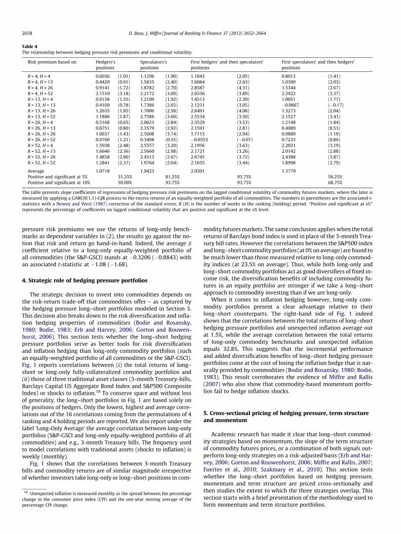
Table 4 reports the averages of the b coefficients from (2) foreach of the hedging pressure risk premiums modeled in Section 3.It is clear from the table that, irrespective of the criterion used toallocate commodities to portfolios, higher conditional volatilityusually leads to higher risk premium. On average, a 1% rise inweekly conditional volatility leads to a 1.6% rise in weekly risk pre-mium across the various single and double sorts. This is consistentwith the idea that in periods of high volatility in commodity mar-kets hedgers are willing to pay a higher cost for their insurance.Likewise, speculators demand a risk premium that is proportionateto the price risk they take on. If in place of the long–short hedging

Table 4The relationship between hedging pressure risk premiums and conditional volatility.

Risk premium based on Hedgers’spositions

Speculators’spositions

First hedgers’ and then speculators’positions

First speculators’ and then hedgers’positions

R = 4, H = 4 0.6036 (1.01) 1.1296 (1.90) 1.1843 (2.05) 0.8013 (1.41)R = 4, H = 13 0.4429 (0.91) 1.5835 (2.40) 1.6084 (2.63) 1.0390 (2.03)R = 4, H = 26 0.9141 (1.72) 1.8782 (2.70) 2.8587 (4.31) 1.5344 (2.67)R = 4, H = 52 2.1510 (3.18) 2.2172 (3.09) 2.6556 (3.89) 2.2922 (3.37)R = 13, H = 4 0.9158 (1.55) 1.2109 (1.92) 1.4513 (2.30) 1.0051 (1.77)R = 13, H = 13 0.4169 (0.78) 1.7386 (2.65) 2.1251 (3.05) �0.0867 (�0.17)R = 13, H = 26 1.2635 (1.85) 1.7006 (2.58) 2.6491 (4.06) 1.3273 (2.04)R = 13, H = 52 1.1806 (1.87) 2.7586 (3.60) 2.5534 (3.50) 2.1527 (3.41)R = 26, H = 4 0.5168 (0.65) 2.0623 (2.84) 2.3529 (3.53) 1.2148 (1.84)R = 26, H = 13 0.6751 (0.80) 2.3579 (2.92) 2.1591 (2.81) 0.4989 (0.53)R = 26, H = 26 1.0637 (1.43) 2.5608 (3.74) 1.7115 (2.94) 0.9880 (1.19)R = 26, H = 52 0.9760 (1.21) 0.3498 (0.55) �0.0353 (�0.07) 0.7233 (0.86)R = 52, H = 4 1.5938 (2.48) 2.5557 (3.20) 2.1956 (3.63) 2.2031 (3.19)R = 52, H = 13 1.6646 (2.36) 2.5660 (2.98) 2.1721 (3.26) 2.0142 (2.88)R = 52, H = 26 1.4858 (2.60) 2.4313 (2.67) 2.6745 (3.72) 2.4388 (3.87)R = 52, H = 52 1.2841 (2.37) 1.9764 (2.64) 2.1655 (3.44) 1.8998 (2.79)

Average 1.0718 1.9423 2.0301 1.3779Positive and significant at 5% 31.25% 81.25% 93.75% 56.25%Positive and significant at 10% 50.00% 93.75% 93.75% 68.75%

The table presents slope coefficients of regressions of hedging pressure risk premiums on the lagged conditional volatility of commodity futures markets, where the later ismeasured by applying a GARCH(1,1)-GJR process to the excess returns of an equally-weighted portfolio of all commodities. The numbers in parentheses are the associated t-statistics with a Newey and West (1987) correction of the standard errors. R (H) is the number of weeks in the ranking (holding) period. ‘‘Positive and significant at x%’’represents the percentage of coefficients on lagged conditional volatility that are positive and significant at the x% level.

2658 D. Basu, J. Miffre / Journal of Banking & Finance 37 (2013) 2652–2664

pressure risk premiums we use the returns of long-only bench-marks as dependent variables in (2), the results go against the no-tion that risk and return go hand-in-hand. Indeed, the average bcoefficient relative to a long-only equally-weighted portfolio ofall commodities (the S&P-GSCI) stands at �0.3206 (�0.8843) withan associated t-statistic at �1.08 (�1.68).

4. Strategic role of hedging pressure portfolios

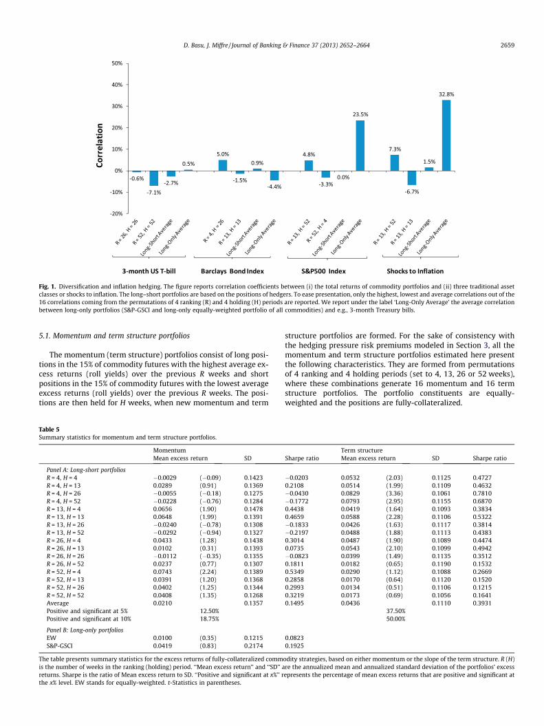
The strategic decision to invest into commodities depends onthe risk-return trade-off that commodities offer – as captured bythe hedging pressure long–short portfolios modeled in Section 3.This decision also breaks down to the risk diversification and infla-tion hedging properties of commodities (Bodie and Rosansky,1980; Bodie, 1983; Erb and Harvey, 2006; Gorton and Rouwen-horst, 2006). This section tests whether the long–short hedgingpressure portfolios serve as better tools for risk diversificationand inflation hedging than long-only commodity portfolios (suchan equally-weighted portfolio of all commodities or the S&P-GSCI).Fig. 1 reports correlations between (i) the total returns of long–short or long-only fully-collateralized commodity portfolios and(ii) those of three traditional asset classes (3-month Treasury-bills,Barclays Capital US Aggregate Bond Index and S&P500 CompositeIndex) or shocks to inflation.18 To conserve space and without lossof generality, the long–short portfolios in Fig. 1 are based solely onthe positions of hedgers. Only the lowest, highest and average corre-lations out of the 16 correlations coming from the permutations of 4ranking and 4 holding periods are reported. We also report under thelabel ‘Long-Only Average’ the average correlation between long-onlyportfolios (S&P-GSCI and long-only equally-weighted portfolio of allcommodities) and e.g., 3-month Treasury bills. The frequency usedto model correlations with traditional assets (shocks to inflation) isweekly (monthly).

Fig. 1 shows that the correlations between 3-month Treasurybills and commodity returns are of similar magnitude irrespectiveof whether investors take long-only or long–short positions in com-

18 Unexpected inflation is measured monthly as the spread between the percentagechange in the consumer price index (CPI) and the one-year moving average of thepercentage CPI change.

modity futures markets. The same conclusion applies when the totalreturns of Barclays bond index is used in place of the 3-month Trea-sury bill rates. However the correlations between the S&P500 indexand long–short commodity portfolios (at 0% on average) are found tobe much lower than those measured relative to long-only commod-ity indices (at 23.5% on average). Thus, while both long-only andlong–short commodity portfolios act as good diversifiers of fixed in-come risk, the diversification benefits of including commodity fu-tures in an equity portfolio are stronger if we take a long–shortapproach to commodity investing than if we are long-only.

When it comes to inflation hedging however, long-only com-modity portfolios present a clear advantage relative to theirlong–short counterparts. The right-hand side of Fig. 1 indeedshows that the correlations between the total returns of long–shorthedging pressure portfolios and unexpected inflation average outat 1.5%, while the average correlation between the total returnsof long-only commodity benchmarks and unexpected inflationequals 32.8%. This suggests that the incremental performanceand added diversification benefits of long–short hedging pressureportfolios come at the cost of losing the inflation hedge that is nat-urally provided by commodities (Bodie and Rosansky, 1980; Bodie,1983). This result corroborates the evidence of Miffre and Rallis(2007) who also show that commodity-based momentum portfo-lios fail to hedge inflation shocks.

5. Cross-sectional pricing of hedging pressure, term structureand momentum

Academic research has made it clear that long–short commod-ity strategies based on momentum, the slope of the term structureof commodity futures prices, or a combination of both signals out-perform long-only strategies on a risk-adjusted basis (Erb and Har-vey, 2006; Gorton and Rouwenhorst, 2006; Miffre and Rallis, 2007;Fuertes et al., 2010; Szakmary et al., 2010). This section testswhether the long–short portfolios based on hedging pressure,momentum and term structure are priced cross-sectionally andthen studies the extent to which the three strategies overlap. Thissection starts with a brief presentation of the methodology used toform momentum and term structure portfolios.

Fig. 1. Diversification and inflation hedging. The figure reports correlation coefficients between (i) the total returns of commodity portfolios and (ii) three traditional assetclasses or shocks to inflation. The long–short portfolios are based on the positions of hedgers. To ease presentation, only the highest, lowest and average correlations out of the16 correlations coming from the permutations of 4 ranking (R) and 4 holding (H) periods are reported. We report under the label ‘Long-Only Average’ the average correlationbetween long-only portfolios (S&P-GSCI and long-only equally-weighted portfolio of all commodities) and e.g., 3-month Treasury bills.

D. Basu, J. Miffre / Journal of Banking & Finance 37 (2013) 2652–2664 2659

5.1. Momentum and term structure portfolios

The momentum (term structure) portfolios consist of long posi-tions in the 15% of commodity futures with the highest average ex-cess returns (roll yields) over the previous R weeks and shortpositions in the 15% of commodity futures with the lowest averageexcess returns (roll yields) over the previous R weeks. The posi-tions are then held for H weeks, when new momentum and term

Table 5Summary statistics for momentum and term structure portfolios.

MomentumMean excess return SD

Panel A: Long-short portfoliosR = 4, H = 4 �0.0029 (�0.09) 0.1423R = 4, H = 13 0.0289 (0.91) 0.1369R = 4, H = 26 �0.0055 (�0.18) 0.1275R = 4, H = 52 �0.0228 (�0.76) 0.1284R = 13, H = 4 0.0656 (1.90) 0.1478R = 13, H = 13 0.0648 (1.99) 0.1391R = 13, H = 26 �0.0240 (�0.78) 0.1308R = 13, H = 52 �0.0292 (�0.94) 0.1327R = 26, H = 4 0.0433 (1.28) 0.1438R = 26, H = 13 0.0102 (0.31) 0.1393R = 26, H = 26 �0.0112 (�0.35) 0.1355R = 26, H = 52 0.0237 (0.77) 0.1307R = 52, H = 4 0.0743 (2.24) 0.1389R = 52, H = 13 0.0391 (1.20) 0.1368R = 52, H = 26 0.0402 (1.25) 0.1344R = 52, H = 52 0.0408 (1.35) 0.1268Average 0.0210 0.1357Positive and significant at 5% 12.50%Positive and significant at 10% 18.75%

Panel B: Long-only portfoliosEW 0.0100 (0.35) 0.1215S&P-GSCI 0.0419 (0.83) 0.2174

The table presents summary statistics for the excess returns of fully-collateralized commis the number of weeks in the ranking (holding) period. ‘‘Mean excess return’’ and ‘‘SD’’ areturns. Sharpe is the ratio of Mean excess return to SD. ‘‘Positive and significant at x%’’ rthe x% level. EW stands for equally-weighted. t-Statistics in parentheses.

structure portfolios are formed. For the sake of consistency withthe hedging pressure risk premiums modeled in Section 3, all themomentum and term structure portfolios estimated here presentthe following characteristics. They are formed from permutationsof 4 ranking and 4 holding periods (set to 4, 13, 26 or 52 weeks),where these combinations generate 16 momentum and 16 termstructure portfolios. The portfolio constituents are equally-weighted and the positions are fully-collateralized.

Term structureSharpe ratio Mean excess return SD Sharpe ratio

�0.0203 0.0532 (2.03) 0.1125 0.47270.2108 0.0514 (1.99) 0.1109 0.4632�0.0430 0.0829 (3.36) 0.1061 0.7810�0.1772 0.0793 (2.95) 0.1155 0.68700.4438 0.0419 (1.64) 0.1093 0.38340.4659 0.0588 (2.28) 0.1106 0.5322�0.1833 0.0426 (1.63) 0.1117 0.3814�0.2197 0.0488 (1.88) 0.1113 0.43830.3014 0.0487 (1.90) 0.1089 0.44740.0735 0.0543 (2.10) 0.1099 0.4942�0.0823 0.0399 (1.49) 0.1135 0.35120.1811 0.0182 (0.65) 0.1190 0.15320.5349 0.0290 (1.12) 0.1088 0.26690.2858 0.0170 (0.64) 0.1120 0.15200.2993 0.0134 (0.51) 0.1106 0.12150.3219 0.0173 (0.69) 0.1056 0.16410.1495 0.0436 0.1110 0.3931

37.50%50.00%

0.08230.1925

odity strategies, based on either momentum or the slope of the term structure. R (H)re the annualized mean and annualized standard deviation of the portfolios’ excessepresents the percentage of mean excess returns that are positive and significant at

Table 6Cross-sectional pricing of hedging pressure, term structure and momentum.

k0 k1

Panel A: Long-short portfoliosHedgers’ hedging pressure 0.0001 (0.47) 0.0008 (3.52)Speculators’ hedging pressure 0.0003 (1.55) 0.0023 (7.66)Hedgers and speculators’ hedging

pressure0.0004 (1.97) 0.0022 (7.17)

Speculators and hedgers’ hedgingpressure

0.0001 (0.75) 0.0008 (3.63)

Momentum 0.0003 (1.57) 0.0005 (1.12)Term structure 0.0003 (1.88) 0.0012 (3.81)

Panel B: Long-only portfoliosEqually-weighted portfolio of all

commodities�0.0001 (�0.11) 0.0005 (0.51)

S&P-GSCI 0.0002 (0.26) 0.0006 (0.46)

The table presents means and Shanken’s (1992) adjusted t-statistics (in parenthe-ses) for the lambda coefficients obtained by estimating step-two Fama and MacBeth(1973) cross-section regressions. For a given signal (e.g., hedgers’ hedging pressure),the lambdas have been pooled across the 16 permutations of 4 ranking and 4holding periods (each set to 4, 13, 26 or 52 weeks).

2660 D. Basu, J. Miffre / Journal of Banking & Finance 37 (2013) 2652–2664

Table 5, Panel A presents summary statistics for the excess re-turns of long–short momentum and term structure portfolios. Un-like previously reported (Erb and Harvey, 2006; Miffre and Rallis,2007), the momentum strategies fail to consistently outperformlong-only positions: over the sample considered (1992–2011), theaverage Sharpe ratio across the 16 momentum portfolios stands atmerely 0.15 (versus 0.19 for the S&P-GSCI in Table 5, Panel B). Relat-edly, only 12.5% (18.75%) of the 16 momentum portfolios consideredearn positive mean excess returns at the 5% (10%) level.

The right-hand side of Table 5 shows that 75% of the 16 termstructure strategies analyzed present Sharpe ratios that are higherthan 0.19, the Sharpe ratio of the S&P-GSCI. This indicates that rollyield is a better signal on which to allocate wealth than long-onlypositions (see also Erb and Harvey, 2006; Gorton and Rouwenhorst,2006). The performance of term structure portfolios however com-pares unfavorably to that of hedging pressure portfolios as re-ported in Tables 2 and 3. For example, while all 64 hedgingpressure portfolios offered Sharpe ratios superior to that of theS&P-GSCI, only 75% of the term structure portfolios considered inTable 5 outperform the S&P-GSCI on a risk-adjusted basis. Besides,the average Sharpe ratio of the term structure portfolios at 0.39 inTable 5 is lower than that of the hedging pressure portfolios at 0.51in Tables 2 and 3. Likewise, the average annualized mean excess re-turn of the term structure portfolios merely equals 4.36% in Table 5versus 5.55% in Tables 2 and 3 for the hedging pressure portfolios.Finally, while 82.81% of the mean excess returns of the long–shorthedging pressure portfolios in Tables 2 and 3 were significant atthe 10% level, that conclusion applies to merely 50% of the termstructure portfolios in Table 5. So the conclusion thus far hints to-wards the superiority of the hedging pressure signal at explainingcommodity futures prices.

9 ln(OIi,t�1) is used as a proxy for size in George and Hwang (2004) and Park (2010).

5.2. Cross-sectional pricing

We use the two-step methodology of Fama and MacBeth (1973)to investigate whether the hedging pressure, momentum and termstructure portfolios explain cross-sectional commodity futures re-turns. The first step consists of time-series regressions of weeklycommodity futures returns on the excess returns of either one ofthe long–short hedging pressure, momentum or term structureportfolios presented in Tables 2, 3 and 5 over a window spanning5 years. The second step entails running the following cross-sec-tional regressions in each of the next k (k = 1, . . . ,52) weeks

ri;tþk ¼ k0;tþk þ k1;tþkb̂i;t þ ti;tþk ð3Þ

b̂i;t is the slope coefficient from the first-step, i = 1, . . . ,N where N isthe number of commodity futures contracts included in the first andsecond steps, ti,t+k is a random error term. This two-stage procedureis applied iteratively until the sample ends. The significance of k0

and k1 is then tested using Shanken’s (1992) corrected t-tests todetermine which factor prices the cross section of commodity fu-tures returns.

As we have 4 ranking and 4 holding periods, we end up with 16long–short portfolios for each of the following six signals: hedgers’hedging pressure, speculators’ hedging pressure, hedgers and spec-ulators’ hedging pressure, speculators and hedgers’ hedging pres-sure, momentum and term structure. The prices of risk obtainedfor the various 16 portfolios are stacked together for each of thesix signals, resulting, as in Table 6, Panel A, in six estimates forthe average intercept (k0) and in six estimates for the average priceof risk (k1). In Table 6, Panel B, we test for the cross-sectional pric-ing of long-only commodity portfolios such as an equally-weightedportfolio of all commodities and the S&P-GSCI.

While momentum is not priced cross-sectionally, the prices ofrisk associated with hedging pressure and term structure are found

to be positive at the 1% level in Table 6, Panel A, with a relativeadvantage for the risk premiums modeled from the positions ofspeculators (in isolation or in conjunction with those of hedgers)and for the signal emanating from the slope of the term structure.Further, the fact that the prices of risk associated with long-onlyportfolios (Table 6, Panel B) are zero at even the 10% level high-lights the need to take both long and short positions (based onhedging pressure or the slope of the term structure) to accuratelycapture the risk premium of commodity futures contracts. A failureto take hedging pressure or inventory considerations into accountresults in the misleading conclusion that there is no risk premiumin commodity futures markets.

5.3. Disentangling the three effects

Tables 2, 3 and 6 show that contracts with low hedgers’ hedgingpressure, high speculators’ hedging pressure, high average rollyields and possibly good past performance outperform contractswith high hedgers’ hedging pressure, low speculators’ hedgingpressure, low average roll yields and possibly poor past perfor-mance. To identify the marginal effect of each signal on commodityfutures prices while controlling for the effect of other signals, weapply to our setting the methodology proposed by George andHwang (2004) and Park (2010). Each week t, we run the followingFama and MacBeth (1973) cross-sectional regressions

Ri;t ¼ b0;t þ b1;tRi;t�1 þ b2;t lnðOIi;t�1Þ þ b3;tHPLHedgi;t�k þ b4;tHPSHedg

i;t�k

þ b5;tHPLSpeci;t�k þ b6;tHPSSpec

i;t�k þ b7;tMomLi;t�k þ b8;tMomSi;t�k

þ b9;tTSLi;t�k þ b10;tTSSi;t�k þ ei;t

k = 1, . . . ,H for a strategy with a H-week holding period(H = {4,13,26,52}), Ri,t is the excess return of commodity futurescontract i in week t, OIi,t�1 is the dollar value of open interest for

contract i in week t � 1,19 HPLHedgi;t�k is a dummy variable equal to 1

(0) if commodity i is included in (excluded from) the long portfolioformed at time t � k that is based on hedgers’ hedging pressure over

the former R weeks (R = {4,13,26,52}), HPSHedgi;t�k is a dummy variable

equal to 1 (0) if commodity i is included in (excluded from) the shortportfolio formed at time t � k that is based on hedgers’ hedging pres-sure over the former R weeks. Likewise, we form two speculators’

1

Table 7Disentangling the effects of hedging pressure, momentum and term structure on commodity futures returns.

One set of dummies only Combination of dummies

(A) (B) (C) (D) (E) (F) (G)

Panel A: Estimated parametersIntercept 0.0020 0.0016 0.0013 0.0012 0.0016 0.0012 0.0020

(3.41) (2.99) (2.36) (2.26) (2.71) (2.09) (3.17)Ri,t�1 0.0094 0.0090 0.0120 0.0106 0.0111 0.0095 0.0099

(3.20) (3.11) (4.21) (3.69) (3.55) (3.09) (3.01)ln(OIi,t�1 �0.0001 �0.0001 �0.0001 �0.0001 �0.0001 �0.0001 �0.0001

(�2.90) (�2.44) (�1.96) (�1.98) (�2.56) (�1.87) (�3.15)

HPLHedgi;t�k

0.0008 0.0007 0.0004

(3.67) (3.07) (1.59)

HPSHedgi;t�k

�0.0008 �0.0003 0.0002

(�4.67) (�1.74) (0.79)

HPLSpeci;t�k

0.0008 0.0006 0.0006

(4.16) (3.02) (2.40)

HPSSpeci;t�k

�0.0013 �0.0008 �0.0009

(�6.80) (�3.67) (�3.36)MomLi,t�k 0.0002 0.0004 0.0001 0.0003

(0.93) (1.50) (0.57) (1.10)MomSi,t�k �0.0003 �0.0003 �0.0004 �0.0003

(�1.49) (�1.24) (�1.47) (�1.29)TSLi,t�k 0.0011 0.0010 0.0011 0.0011

(5.47) (4.33) (5.08) (4.66)TSSi,t�k �0.0008 �0.0005 �0.0004 �0.0003

(�3.81) (�2.12) (�1.92) (�1.36)

Panel B: Annualized mean excess returns of pure fully-collateralized commodity strategiesHedgers’ HP 0.0419 0.0271 0.0058

(6.40) (3.80) (0.66)Speculators’ HP 0.0531 0.0356 0.0374

(8.26) (5.00) (4.20)Momentum 0.0141 0.0182 0.0133 0.0170

(1.75) (2.01) (1.48) (1.75)Term structure 0.0475 0.0380 0.0397 0.0378

(7.16) (4.95) (5.34) (4.62)

The table presents means of slope coefficients from cross-sectional regressions of commodity excess return on their first lag (Ri,t�1), lagged dollar open interest and 8 dummyvariables. HPLHedg

i;t�k is a dummy variable equal to 1 (0) if commodity i is included in (excluded from) the long portfolio based on hedgers’ hedging pressure (HP), HPSHedgi;t�k is a

dummy variable equal to 1 (0) if commodity i is included in (excluded from) the short portfolio based on hedgers’ hedging pressure. HPLSpeci;t�k and HPSSpec

i;t�k are two speculators’hedging pressure dummies, MomLi,t�k and MomSi,t�k are two momentum dummies and TSLi,t�k and TSSi,t�k are two term structure dummies that take values of 1 if commodityi is included in the long (L) or short (S) portfolios based on speculators’ hedging pressure, momentum and term structure and take values of 0, otherwise. t-Statistics inparentheses.

20 This result is consistent with the well-documented negative relationshipidentified in equity markets between liquidity levels and expected returns (Amihudand Mendelson, 1986).

D. Basu, J. Miffre / Journal of Banking & Finance 37 (2013) 2652–2664 2661

hedging pressure dummies HPLSpeci;t�k and HPSSpec

i;t�k, two momentumdummies MomLi,t�k and MomSi,t�k and two term structure dummiesTSLi,t�k and TSSi,t�k. For example, MomLi,t�k equals 1 (0) if commodityi is included in (excluded from) the long momentum portfolioformed at time t � k that is based on performance over the formerR weeks. Similarly, TSSi,t�k equals 1 (0) if commodity i is includedin (excluded from) the short term structure portfolio formed at timet � k based on roll yields over the previous R weeks. Finally, ei,t is anerror term and bj,t are the j = 0, . . . ,10 parameters to estimate. Wethen compute t-statistics for the resulting bj,t coefficients to testthe marginal effect of each signal on commodity futures returns. Fol-lowing George and Hwang (2004) and Park (2010), we interpret the

differences ðb̂3;t � b̂4;tÞ=2; ðb̂5;t � b̂6;tÞ=2; ðb̂7;t � b̂8;tÞ=2 and

ðb̂9;t � b̂10;tÞ=2 as the weekly excess returns of fully-collateralizedpure hedgers’ hedging pressure, pure speculators’ hedging pressure,pure momentum and pure term structure strategies, respectively.

Table 7 presents the mean of the estimated bj,t coefficients inPanel A and the annualized mean excess returns of pure commod-ity strategies in Panel B. Alongside with lagged returns and lagged$OI, regressions (A) to (D) use one set of dummies as regressors,while regressions (E) to (G) use more than one set of dummies asregressors. b1 is positive at the 1% level, indicating the presenceof first-order serial correlation over short-horizons (as in Kat andOomen, 2007). b2 is negative and significant at the 10% level or

better, suggesting that relatively less liquid contracts with lowerdollar value of open interests earn higher mean returns.20

As expected, the estimated bj,t coefficients for j = 3, . . . ,10 inmodels (A) to (D) are positive and often significant for the longdummies, an indication that the commodities included in theselong portfolios appreciated in value, even after accounting forlagged returns and lagged open interest. Vice versa, the estimatedbj,t coefficients are negative and often significant for the short dum-mies, a sign that the commodities included in these short portfoliosdepreciated in value. The annualized mean excess returns of purefully-collateralized long–short strategies reported in Table 7, PanelB range from 1.41% (t-statistic of 1.75) for the pure momentum sig-nal to 5.31% (t-statistic of 8.26) for the pure speculators’ hedgingpressure signal. The results thus show that, even after accountingfor lagged returns and lagged $OI, the pure term structure andhedging pressure strategies are profitable. The momentum signalperforms the worst. These results scare well with the analysis per-formed in Tables 2, 3, 5 and 6.

Models (E) to (F) capture the role of one signal (e.g., hedgers’hedging pressure) after controlling for the other signals (e.g., termstructure and momentum). This is done by including more than

2662 D. Basu, J. Miffre / Journal of Banking & Finance 37 (2013) 2652–2664

one set of dummies in the cross-sectional regressions. Model (E)shows that profits from the pure hedgers’ hedging pressure strat-egy persists after accounting for the performance of both momen-tum and term structure strategies (as demonstrated by b̂3;t > 0,b̂4;t < 0 in Panel A and by ðb̂3;t � b̂4;tÞ=2 > 0 in Panel B). The sameconclusion applies to the pure speculators’ hedging pressure strat-egy in model (F). Albeit slightly reduced compared to the mean ex-cess returns reported in Table 2, profits from hedging pressurestrategies are still significant when commodity futures returnsare controlled for lagged returns, lagged $OI and the returns pre-dicted from momentum and term structure signals. It follows thatthe predictive power of hedging pressure over future commodityexcess returns is different from the forecasting power of (i) past re-turns and (ii) the slope of the term structure. In relative terms, thepure term structure signal and pure speculators’ hedging pressuresignal generate profits in Panel B that are more sizeable than thoseemanating from hedgers’ hedging pressure or momentum.

When all four sets of dummies are included in the cross-sectionalmodel (G) in Table 7, Panel A, b̂5;t and b̂6;t for the long and short spec-ulators’ hedging pressure dummies and b̂9;t for the long term struc-ture dummy are the only coefficients that are significant at the 5%level. Likewise, the results from Panel B show that the mean excessreturns of pure speculators’ hedging pressure and pure term struc-ture portfolios are sizeable both in economic term (3.74% and3.78% a year, respectively) and in statistical term (the associatedt-statistics are 4.20 and 4.62, respectively). This shows that thepositions of speculators and the slope of the term structure are inde-pendent drivers of commodity futures returns. As the slope of theterm structure of commodity futures prices is considered as proxyfor inventory levels (Working, 1949; Brennan, 1958), we concludethat commodity futures risk premiums depend on considerationsrelating to both speculators’ hedging pressure and inventory levels.

By contrast, none of the hedgers’ hedging pressure dummies ispriced cross-sectionally in Table 7, Panel A, model (G) and themean excess returns of pure hedgers’ hedging pressure portfoliosequals zero in statistical term in Table 7, Panel B. The results ofmodels (A), (E) and (G) therefore suggest that the predictive powerof hedgers’ hedging pressure over future excess returns in models(A) and (E) derives from that of speculators’ hedging pressure: oncethe later is properly accounted for, the former disappears. Findingthat out of the two hedging pressure signals, the one derived fromthe positions of speculators dominates the one based on the posi-tions of hedgers suggests that, as hypothesized by Working (1958)and Chang (1985), speculators earn a risk premium as compensa-tion both for providing risk-bearing capacity to hedgers and foridentifying profitable opportunities.

Finally, the momentum strategy fails to dominate any other sig-nal: when the term structure and hedging pressure dummies areincluded in the cross-sectional model (G), none of the momentumdummies is priced in Table 7, Panel A and the mean excess returnof the pure momentum strategy in Table 7, Panel B is found to beone of the lowest reported (at 1.70% a year with a t-statistic of1.75). Barberis et al. (1998), Daniel et al. (1998) and Hong and Stein(1999) view the profitability of momentum strategies as a manifes-tation of behavioral biases. Finding as in Tables 6 and 7 thatmomentum is not priced, when term structure and hedging pres-sure are, indicates that rational pricing relating to hedging demandand inventory considerations is more likely to drive commodity fu-tures risk premiums than cognitive errors made while incorporat-ing information into prices.

6. Conclusions

We construct factor mimicking portfolios to capture the effectof systematic hedging pressure on the risk premium of commodity

futures contracts. The long–short portfolios we then form buycommodity contracts for which hedgers are particularly shortand speculators particularly long and sell commodity contractsfor which hedgers are particularly long and speculators particu-larly short. Our fully-collateralized hedging pressure portfoliospresent Sharpe ratios that range from 0.27 to 0.93 with an averageat 0.51. By contrast, over the same period (1992–2011), a long-onlyequally-weighted portfolio made of the same 27 commodity fu-tures contracts presents a Sharpe ratio of 0.08 only. The Sharpe ra-tio of the S&P-GSCI stands at merely 0.19. These results suggestthat systematic hedging pressure is a significant determinant ofcommodity futures risk premiums.

Further results can be summarized as follows. First, in line withthe notion that higher risk should be rewarded by higher returns,we find a positive relationship between our hedging pressure riskpremiums and the lagged conditional volatility of commodity fu-tures markets. Second, the hedging pressure portfolios are foundto be better suited at diversifying equity risk than long-only com-modity portfolios, but fail to hedge inflation shocks. Third, ourcross-sectional results show that hedging pressure (and the slopeof the term structure) command positive and significant risk pre-miums, while the prices of risk associated with long-only bench-marks are zero, both statistically and economically. Fourth, thepredictive power of hedging pressure over future commodity ex-cess returns is shown to be different from the forecasting powerof (i) past returns and (ii) the slope of the term structure. Out ofall the signals considered (hedgers’ and speculators’ hedging pres-sures, past performance and past roll yields), the positions of spec-ulators and the slope of the term structure are found to be the mostimportant drivers of commodity futures returns. This leads us tothe conclusion that commodity futures risk premiums depend onconsiderations relating to both speculators’ hedging pressure andinventory levels.

Overall our paper contributes to the recent literature (Acharyaet al., 2010; Hong and Yogo, 2012; Tang and Xiong, 2012; Gortonet al., 2013) that examines the role of systematic factors whichinfluence the cross section of commodity prices. It would be inter-esting to analyze the relationship between our long–short hedgingpressure portfolios and those based on inventory considerations, inorder to further study the link between hedging pressure- andstorage-based theories. Our dynamic long–short portfolios couldalso provide useful benchmarks for analyzing the performance ofcommodity trading advisers and, more generally, any hedge fundwith commodity exposure. We see these issues as interesting ave-nues for future research.

Acknowledgements

The authors would like to thank an anonymous referee, ChrisBrooks, Adrian Fernandez-Perez, Ana-Maria Fuertes, AbrahamLioui, Zenu Sharma and participants at the the EDHEC-Risk Alter-native Investments Days 2010 and at a research seminar at EDHECBusiness School for helpful comments. The usual disclaimerapplies.

Appendix A. Constituents of hedging pressure portfolios andsummary statistics on hedging pressure

The appendix presents the percentages of times each commod-ity enters the long hedgers’ hedging pressure portfolios (xLong) andthe short hedgers’ hedging pressure portfolios (xShort), summarystatistics on hedgers’ hedging pressure and average roll yieldsper commodity. t-Statistics for the hypothesis that the correlationis zero are in parentheses.

xLong (%) xShort (%) Hedgers’ hedging pressure Average roll yields (%)

Average StDev Minimum Maximum

Panel A: Individual commoditiesCocoa 0.00 13.11 0.45 0.06 0.28 0.64 �1.38Coffee 5.73 1.89 0.43 0.07 0.21 0.62 �1.56Copper 4.73 18.53 0.45 0.10 0.16 0.67 0.09Corn 0.00 34.75 0.50 0.07 0.34 0.69 �2.40Cotton 0.66 32.23 0.49 0.10 0.27 0.72 �1.59Crude oil 0.00 13.75 0.49 0.03 0.40 0.59 0.05Electricity 0.00 0.00 0.47 0.03 0.39 0.52 �2.02Feeder cattle 1.67 70.17 0.57 0.12 0.09 0.84 0.05Gasoline 0.00 3.12 0.45 0.05 0.31 0.59 �0.55Gold 40.81 27.27 0.39 0.15 0.16 0.75 �0.55Heating oil 0.03 0.39 0.46 0.04 0.35 0.55 �0.16Lean hogs 2.76 37.98 0.50 0.10 0.26 0.83 �2.60Live cattle 0.00 12.33 0.48 0.06 0.31 0.59 �0.44Lumber 29.48 24.13 0.40 0.20 0.00 1.00 �2.06Natural gas 0.00 19.65 0.50 0.06 0.38 0.68 �1.41Oats 52.91 0.00 0.33 0.09 0.09 0.57 �1.58Orange 13.44 7.17 0.39 0.11 0.06 0.65 �1.73Palladium 57.55 7.60 0.32 0.16 0.06 0.80 �0.04Platinum 72.62 0.16 0.26 0.13 0.04 0.65 0.29Pork bellies 14.98 25.26 0.50 0.20 0.02 1.00 �0.21Rough rice 7.94 4.71 0.43 0.12 0.16 0.72 �2.29Silver 84.73 0.00 0.26 0.08 0.05 0.47 �0.55Soybeans 5.28 17.68 0.44 0.10 0.17 0.68 �0.19Soybean meal 6.35 2.52 0.41 0.07 0.22 0.63 0.59Soybean oil 5.79 8.41 0.43 0.09 0.20 0.64 �0.67Sugar 6.03 7.86 0.43 0.08 0.20 0.67 0.07Wheat 2.65 19.15 0.47 0.09 0.18 0.64 �2.03

Panel B: Correlations between summary statistics for hedging pressure (roll-yields) andxLong �0.90 0.42 �0.66 �0.04 0.20

(�10.18) (2.30) (�4.37) (�0.21) (1.02)xShort 0.62 0.32 �0.05 0.61 �0.12

(3.93) (1.68) (�0.26) (3.82) (�0.58)

D. Basu, J. Miffre / Journal of Banking & Finance 37 (2013) 2652–2664 2663

References

Acharya, V., Lochstoer, L., Ramadorai, T., 2010. Does Hedging Affect CommodityPrices: The Role of Producer Default Risk. Working Paper, London BusinessSchool.

Amihud, Y., Mendelson, H., 1986. Asset pricing and the bid-ask spread. Journal ofFinancial Economics 17, 223–249.

Anderson, R., Danthine, J.-P., 1981. Cross-hedging. Journal of Political Economy 89,1182–1196.

Barberis, N., Schleifer, A., Vishny, R., 1998. A model of investor sentiment. Journal ofFinancial Economics 49, 307–343.

Bessembinder, H., 1992. Systematic risk, hedging pressure and risk premiums infutures markets. Review of Financial Studies 5, 637–667.

Bhardwaj, G., Gorton, G., Rouwenhorst, K. G., 2008. You Can Fool Some of the PeopleAll of the Time: The Inefficient Performance and Persistence of CommodityTrading Advisors. Yale ICF Working Paper No 08–21.

Bodie, Z., 1983. Commodity futures as a hedge against inflation. Journal of PortfolioManagement, 12–17.

Bodie, Z., Rosansky, V., 1980. Risk and return in commodity futures. FinancialAnalysts Journal, 27–39.

Brennan, M., 1958. The supply of storage. American Economic Review 47, 50–72.Carter, C., Rausser, G., Schmitz, A., 1983. Efficient asset portfolios and the theory of

normal backwardation. Journal of Political Economy 91, 319–331.Chang, E., 1985. Return to speculators and the theory of normal backwardation.

Journal of Finance 40, 193–208.Cootner, P., 1960. Returns to speculators: Telser vs. Keynes. Journal of Political

Economy 68, 396–404.Cootner, P., 1967. Speculation and hedging. Food Research Institute Studies 7, 65–

105.

Daniel, K., Hirshleifer, D., Subrahmanyam, A., 1998. Investor psychology andsecurity market under- and overreactions. Journal of Finance 53, 1839–1885.

DeRoon, F., Nijman, T., Veld, C., 2000. Hedging pressure effects in futures markets.Journal of Finance 55, 1437–1456.

Dusak, K., 1973. Futures trading and investor returns: an investigation ofcommodity market risk premiums. Journal of Political Economy 81, 1387–1406.

Ederington, L., Lee, J.H., 2002. Who trades futures and how: evidence from theheating oil futures market. Journal of Business 75, 353–373.

Erb, C., Harvey, C., 2006. The strategic and tactical value of commodity futures.Financial Analysts Journal 62 (March/April), 69–97.

Fama, E.F., MacBeth, J.D., 1973. Risk, return and equilibrium: empirical tests. Journalof Political Economy 71, 607–636.

Fuertes, A.-M., Miffre, J., Rallis, G., 2010. Tactical allocation in commodity futuresmarkets: combining momentum and term structure signals. Journal of Bankingand Finance 34 (10), 2530–2548.

George, T.J., Hwang, C.Y., 2004. The 52 week high and momentum investing. Journalof Finance 59, 2145–2175.

Glosten, L.R., Jagannathan, R., Runkle, D.E., 1993. On the relation between theexpected value and the volatility of the nominal excess return on stocks. Journalof Finance 48, 1779–1801.

Gorton, G., Hayashi, F., Rouwenhorst, G., 2013. The fundamentals of commodityfutures returns. Review of Finance 17 (1), 35–105

Gorton, G., Rouwenhorst, G., 2006. Facts and fantasies about commodity futures.Financial Analysts Journal 62 (March/April), 47–68.

Hicks, J., 1939. Value and Capital. Oxford University Press.Hirshleifer, D., 1989. Determinants of hedging and risk premia in commodity

futures markets. Journal of Financial and Quantitative Analysis 24, 313–331.Hirshleifer, D., 1990. Hedging pressure and future price movements in a general

equilibrium model. Econometrica 58, 441-28.

2664 D. Basu, J. Miffre / Journal of Banking & Finance 37 (2013) 2652–2664

Hong, H., Stein, J., 1999. A unified theory of underreaction, momentum trading andoverreaction in asset markets. Journal of Finance 54, 2143–2184.

Hong, H., Yogo, M., 2012. What does futures market interest tell us about themacroeconomy and asset prices? Journal of Financial Economics 105, 473–490.

Houthakker, H., 1957. Can speculators forecast prices? Review of Economic andStatistics 39, 143–151.

Kat, H., Oomen, R., 2007. What every investor should know about commodities I:Univariate return analysis. Journal of Investment Management 5, 4–28.

Keynes, J., 1930. Treatise on Money. Macmillan, London.Khan, S., Khoker, Z., Simin, T., 2008. Expected Commodity Futures Return. Working

Paper, University of Western Ontario.Litzenberger, R., Rabinowitz, N., 1995. Backwardation in oil futures markets: theory

and empirical evidence. Journal of Finance 50, 1517–1545.Miffre, J., Rallis, G., 2007. Momentum strategies in commodity futures markets.

Journal of Banking and Finance 31 (6), 1863–1886.Newey, W.K., West, K.D., 1987. Hypothesis testing with efficient method of

moments estimation. International Economic Review 28, 777–787.

Park, S.-C., 2010. The moving average ratio and momentum. Financial Review 45,415–447.

Routledge, B., Seppi, D., Spatt, C., 2000. Equilibrium forward curves for commodities.Journal of Finance 55, 1297–1338.

Rouwenhorst, K.G., Tang, K., 2012. Commodity investing. Annual Review ofFinancial Economics 4, 447–467.

Shanken, J., 1992. On the estimation of beta-pricing models. Review of FinancialStudies 5, 1–33.

Shen, Q., Szakmary, A., Sharma, S., 2007. An examination of momentum strategies incommodity futures markets. Journal of Futures Markets 27, 227–256.

Szakmary, A., Shen, Q., Sharma, S., 2010. Trend-following strategies in commodityfutures: a re-examination. Journal of Banking and Finance 34, 409–426.

Tang, K., Xiong, W., 2012. Index Investment and the Financialization ofCommodities, Financial Analysts Journal, 68 (6), 54–74.

Working, H., 1949. The theory of the price of storage. American Economic Review39, 1254–1266.

Working, H., 1958. A theory of anticipatory prices. American Economic Review 48,1188–1199.