Carbon-based ocean productivity and phytoplankton physiology

from space

Michael J. Behrenfeld,1,2 Emmanuel Boss,3 David A. Siegel,4 and Donald M. Shea5

Received 21 May 2004; revised 19 October 2004; accepted 2 November 2004; published 25 January 2005.

[1] Ocean biogeochemical and ecosystem processes are linked by net primary production(NPP) in the ocean’s surface layer, where inorganic carbon is fixed by photosyntheticprocesses. Determinations of NPP are necessarily a function of phytoplankton biomass andits physiological status, but the estimation of these two terms from space has remained anelusive target. Here we present new satellite ocean color observations of phytoplanktoncarbon (C) and chlorophyll (Chl) biomass and show that derived Chl:C ratios closely followanticipated physiological dependencies on light, nutrients, and temperature. With this newinformation, global estimates of phytoplankton growth rates (m) and carbon-based NPP aremade for the first time. Compared to an earlier chlorophyll-based approach, our carbon-based values are considerably higher in tropical oceans, show greater seasonality at middleand high latitudes, and illustrate important differences in the formation and demise ofregional algal blooms. This fusion of emerging concepts from the phycological and remotesensing disciplines has the potential to fundamentally change how we model and observecarbon cycling in the global oceans.

Citation: Behrenfeld, M. J., E. Boss, D. A. Siegel, and D. M. Shea (2005), Carbon-based ocean productivity and phytoplankton

physiology from space, Global Biogeochem. Cycles, 19, GB1006, doi:10.1029/2004GB002299.

1. Introduction

[2] Marine net primary production (NPP: mg C m�2) is akey metric of ecosystem health and carbon cycling and iscommonly estimated as the product of plant biomass,incident solar flux, and a scaling parameter that accountsfor variations in plant physiology [Behrenfeld et al., 2001].Satellite measurements now routinely provide global chlo-rophyll biomass (Chl) and incident light (I0) data, but theremote determination of phytoplankton carbon (C) biomassand physiological status has proven elusive. Present-dayocean NPP estimates consequently use chlorophyll asan index of phytoplankton biomass and rely on stylizedempirical descriptions of physiological variability [e.g.,Longhurst, 1995; Behrenfeld and Falkowski, 1997a] thatperform poorly when compared to local field measurements[Siegel et al., 2001; Campbell et al., 2002; Behrenfeld et al.,2002]. Far more is known, however, regarding the nature ofphytoplankton physiology than is reflected in these empir-ical relationships. In particular, laboratory studies have longshown that phytoplankton respond to changes in light,

nutrients, and temperature conditions by adjusting cellularpigment levels to match their new demands for photosyn-thesis and that this response is well quantified by changes inthe ratio of chlorophyll to carbon biomass (Chl:C) [e.g.,Geider, 1987; Sakshaug et al., 1989; MacIntyre et al.,2002]. It follows, therefore, that a remote sensing index ofChl:C may provide a path for assessing phytoplanktonphysiology from space.[3] Optical scattering coefficients in marine waters covary

with the suspended particle load (see review by Babin et al.[2003]). Indeed, the particulate beam attenuation coefficientat 660 nm (cp) (an inherent optical property that is domi-nated by scattering) has been repeatedly shown in the fieldto covary with the particulate organic carbon concentration(POC) [Gardner et al., 1993, 1995; Walsh et al., 1995;Loisel and Morel, 1998; Bishop, 1999; Bishop et al., 1999;Claustre et al., 1999]. Behrenfeld and Boss [2003] sug-gested that cp should likewise be well correlated withphytoplankton carbon biomass, particularly since the parti-cle size domain dominating cp more closely matches that ofphytoplankton than POC. Accordingly, they proposed thecp:Chl ratio as an index of phytoplankton C:Chl andsubsequently demonstrated a first-order correspondencebetween cp:Chl and independent 14C-tracer measures ofphysiological condition [Behrenfeld and Boss, 2003]. Thusthe ratio of chlorophyll to light scattering appears to providean optical index of phytoplankton physiology.[4] Currently, cp is not a remote sensing product. However,

recent advances in satellite ocean color data analysis nowpermit the separation of light absorbing and scattering com-ponents in seawater, yielding simultaneous estimates of Chland particulate backscattering coefficients (bbp) [Maritorena

GLOBAL BIOGEOCHEMICAL CYCLES, VOL. 19, GB1006, doi:10.1029/2004GB002299, 2005

1National Aeronautic and Space Administration, Goddard Space FlightCenter, Greenbelt, Maryland, USA.

2Now at Department of Botany and Plant Pathology, Oregon StateUniversity, Corvallis, Oregon, USA.

3School of Marine Sciences, University of Maine, Orono, Maine, USA.4Institute for Computational Earth System Science, University of

California, Santa Barbara, California, USA.5Science Applications International Corporation, NASA Goddard Space

Flight Center, Greenbelt, Maryland, USA.

Copyright 2005 by the American Geophysical Union.0886-6236/05/2004GB002299$12.00

GB1006 1 of 14

et al., 2002; Siegel et al., 2002; Stramski et al., 1999; Loisel etal., 2001]. While bbp is likely more influenced by particlesoutside the phytoplankton size domain than cp [Morel andAhn, 1991; Stramski and Kiefer, 1991], a relationshipbetween bbp and phytoplankton carbon is neverthelessanticipated so long as the abundance of non-algalparticles contributing to bbp covaries with phytoplanktonbiomass. Such covariability in components of the particleassemblage is evidenced by the relatively constant slopeof the particle size spectrum in open ocean waters[Bader, 1970; Stramski and Kiefer, 1991; Kiefer andBerwald, 1992] (see also discussion by Twardowski etal. [2001]) and is responsible for reported correlationsbetween satellite bbp and field measurements of POC[Stramski et al., 1999; Loisel et al., 2001].[5] Here we proceed through a sequence of steps that lead

from satellite Chl and bbp determinations to global carbon-based estimates of ocean NPP. From bbp, we estimate phyto-plankton carbon biomass (C) and then demonstrate thatregional satellite Chl:C ratios behave in a manner consistentwith well-established physiological dependencies on light,nutrients, and temperature.We then useChl:C data to estimatephytoplankton growth rates (m) and, finally, calculate NPPfrom the product of m and C. In this manner, closure on theproductivity equation is achieved through remote sensing,yielding a new view of global ocean productivity and itsvariation over space and time.

2. Methods

2.1. Global Data

[6] Chlorophyll concentrations (Chl: mg m�3) and bbp at440 nm (m�1) were estimated using the Garver-Siegel-Maritorena (GSM) semi-analytical algorithm [Garver andSiegel,1997; Maritorena et al., 2002; Siegel et al., 2002]and monthly satellite water-leaving radiances for the Sep-tember 1997 to January 2002 period from the fourthreprocessing of the Sea-viewing Wide Field-of-view Sensor(SeaWiFS) data set. The GSM algorithm provides chloro-phyll products that compare equally well with coincidentopen ocean observations as chlorophyll products from thestandard SeaWifs algorithm (D. M. Siegel et al., Indepen-dence and interdependences of global ocean optical prop-erties viewed using satellite color imagery, submitted toJournal of Geophysical Research, 2004). For this analysis,we also used coincident SeaWiFS cloud-corrected surfacePAR data (I0: moles photons m�2 h�1), SeaWiFS mixedlayer light attenuation coefficients at 490 nm (k490: m

�1),8-km advanced very high resolution radiometer(AVHRR) sea surface temperature data (SST; �C) fromthe Physical Oceanography Distributed Active ArchiveCenter (PODAAC) (http://podaac-www.jpl.nasa.gov), andmonthly mean regional mixed layer depths (MLD: m) fromthe Fleet Numeric Meteorology and Oceanography Center(FNMOC) (Monterey, California). While FNMOC andclimatological MLD data compare favorably over largespace scales and timescales, the FNMOC model assimilatescoincident field and satellite temperature and salinity dataand thus provides information on interannual variability inMLDs. I0, k490, and MLD data were used to calculate

monthly median mixed layer light levels (Ig) following:Ig = I0 exp

�k490�MLD/2.

2.2. Regional Binning

[7] Arctic and coastal regions were excluded from ouranalysis, and the remaining data (89% of the global oceans)were partitioned into 28 regional bins, defined by ocean basinand the degree of seasonal variability in chlorophyll. Standarddeviations in Chl (s.d.Chl) provide a means to coarselyseparate functionally different ocean regions (e.g., oligotro-phic versus seasonal bloom areas) [Esaias et al., 1999;Doney et al., 2003]. For the current study, five chlorophyllvariance bins (L0 to L4) were used and defined as: L0 =0 < s.d.Chl < 0.018 mg Chl m�3, L1 = 0.018 < s.d.Chl <0.026 mg Chl m�3, L2 = 0.026 < s.d.Chl < 0.09 mg Chlm�3, L3 = 0.09 < s.d.Chl < 0.4 mg Chl m�3, and L4 =s.d.Chl > 0.4 mg Chl m�3. The precise cutoff values forthese bins are not critical and were simply chosen to yieldregions consistent with large-scale ocean circulation andpigment features. All data for the Southern Ocean weregrouped into a single bin because >90% of the data fellinto L2 and L3 variance levels and the seasonal patterns inthese bins were nearly identical.

2.3. Phytoplankton Carbon

[8] To constrain our satellite-based phytoplankton carbonestimates, we analyzed laboratory data compiled byBehrenfeld et al. [2002] on light- and nutrient-dependentchanges in cellular pigmentation from published studiesbetween 1946 and 1987. This data set yielded Chl:C valuesranging from 0.001 to >0.06 mg mg�1, with a median valueof 0.010 mg mg�1 for light levels between 0.7 and1.4 moles photons m�2 h�1. The median mixed layer Ig forour remote sensing data set was 1.2 moles photons m�2 h�1.[9] As an additional constraint, satellite-based POC con-

centrations were calculated from bbp data as the average ofrelationships developed for the Mediterranean (POC =37550 bbp(550) + 1.3 = 29769 bbp(440) + 1.3) [Loisel etal., 2001] and the Antarctic Polar Front Zone (POC =17069 bbp(510)

0.859 = 14726 bbp(440)0.859) [Stramski et

al., 1999], where the first equation is the original pub-lished relationship and the second equation is the con-verted relationship for use with bbp(440) data. We thencalculated phytoplankton carbon:POC ratios for our re-mote sensing data and compared these to field-derivedvalues. Specifically, Eppley et al. [1992] reported phyto-plankton carbon:POC ratios of 29% to 49%, DuRand etal. [2001] found a relatively constant value of 33%throughout the year near Bermuda, Gundersen et al.[2001] reported a value of 32%, and Oubelkheir [2001]measured values ranging from 19% to 21% in regionsspanning from oligotrophic to eutrophic. It is noteworthythat this restricted variability observed in the fieldincludes methodological differences for estimating phyto-plankton carbon.

2.4. Productivity Calculations

[10] For comparative purposes, global ocean NPP wascalculated using our new carbon-based approach and a

GB1006 BEHRENFELD ET AL.: PHYTOPLANKTON GROWTH RATES AND OCEAN PRODUCTIVITY

2 of 14

GB1006

common chlorophyll-based algorithm, the Vertically Gen-eralized Production Model (VGPM) [Behrenfeld andFalkowski, 1997a]. The depth-integrated VGPM equationis NPP = Chl � Zeu � f (I0) � d.l. � Popt

b , where Zeu is thedepth of the photosynthetically active surface layer andphysiological variability (Popt

b ) is described by an empiricalpolynomial function of SST that increases from 0� to 20�Cand then decreases at higher temperatures [Behrenfeld andFalkowski, 1997a]. For both the chlorophyll- and carbon-based calculations, the light-dependent function wasdescribed as, f (I0) = 0.66125 I0/(I0 + 4.1) [Behrenfeld andFalkowski, 1997a], Zeu was calculated as Zeu = ln(0.01)/k490(which gives slightly higher NPP values than earlier VGPMestimates), and the same GSM satellite chlorophyll esti-mates were used.

3. Results

3.1. Satellite-Based Phytoplankton Carbon Biomass

[11] Comparison of monthly bbp and Chl data revealedtwo distinct regimes: one where bbp is relatively constantand one where bbp covaries with Chl (Figure 1). In the mostunproductive ocean regions, bbp varies by only a factor of1.6 (from 0.0010 to 0.0016 m�1) while Chl ranges from0.03 to 0.14 mg m�3 (i.e., a factor of 4.6), with nocorrelation between the two variables (Figure 1). In moreproductive regions where chlorophyll concentrations exceed�0.14 mg Chl m�3, bbp and Chl are well correlated (r2 =0.74) (Figure 1). Our interpretation of this bilinear pattern isthat Chl variability is largely due to intracellular changes inpigmentation (i.e., physiology) in impoverished oceanregions, while in more enriched regions, first-order changesin Chl and bbp are predominantly due to changes inphytoplankton biomass (i.e., abundance).[12] To estimate phytoplankton carbon biomass (mg m�3)

from bbp, we first subtracted a background valueof 0.00035 m�1 and then multiplied by a scalar of13,000 mg C m�2 (i.e., phytoplankton C = 13,000 �(bbp � 0.00035)). The background value was estimatedfrom least squares regression analysis of the linear portionof the Chl-bbp relationship (Figure 1, solid line), and itrepresents a global estimate of backscattering by the stableheterotrophic and detrital components of the surface particlepopulation. For comparison, a similar independent estimateof 0.00017 m�1 is calculated using backscattering coeffi-cients from Stramski and Kiefer [1991] and a field-basedbackground heterotrophic bacterial concentration of 7 �1011 m�3 from Cho and Azam [1990, Figure 1]. The scalar of13,000 mg C m�2 was chosen to give satellite Chl:C values(average = 0.010, range = 0.002 to 0.030) consistent withlaboratory results and an average phytoplankton contributionto total particulate organic carbon of �30% (range: 24% to37%), which is consistent with field estimates from a varietyof ocean regions [Eppley et al., 1992; DuRand et al., 2001;Gundersen et al., 2001; Oubelkheir, 2001] (see section 2.3).[13] Restating the above in more general terms, we

assume that the particle population contributing to bbp iscomprised of a stable non-algal ‘‘background’’ componentand a second component that includes phytoplankton andother particles that covary with phytoplankton. We then

subtract the ‘‘background’’ component and directly relatethe remaining bbp to phytoplankton biomass using a simplescalar that gives reasonable values for both Chl:C and thephytoplankton carbon to POC ratio. We do not assume thatthe remaining bbp is entirely due to backscattering byphytoplankton, only that it correlates with phytoplanktonabundance. This conversion of bbp to phytoplankton carbonwill clearly be compromised by significant shifts in thecomposition of the particle assemblage (e.g., prominentinorganic particulate component) or by large deviations inthe slope of the particle size spectrum. The influence oflocal-scale variability in such factors has been minimizedin the current analysis by integrating monthly data overlarge areas and omitting coastal waters where suspendedinorganic particle loads can be particularly high (seesection 2.2).[14] In the next two sections, we describe how regional

variability in satellite Chl:C is consistent with anticipatedchanges in phytoplankton physiology. Importantly, theseresults are quite insensitive to the bbp-to-carbon conversionparameters described above, such that the same degree ofcorrespondence with mixed layer growth conditions isfound with unaltered Chl:bbp ratios as with our convertedChl:C values.

3.2. Five Basic Seasonal Patterns in PhytoplanktonBiomass and Physiology

[15] Analysis of regional phytoplankton Chl, C, andChl:C ratios revealed seasonal patterns related to basic

Figure 1. Regional monthly mean particulate backscatter-ing coefficients at 440 nm (bbp) and surface chlorophyllconcentrations (Chl) for the September 1997 to January2002 period. Data are from the 28 regional bins identified inFigure 2a. The solid line represents a linear fit to data withChl > 0.14 mg m�3. The dashed line indicates the mean bbpvalue of 0.0012 m�1 for data where Chl < 0.14 mg m�3

(i.e., the realm where Chl and bbp are uncorrelated).

GB1006 BEHRENFELD ET AL.: PHYTOPLANKTON GROWTH RATES AND OCEAN PRODUCTIVITY

3 of 14

GB1006

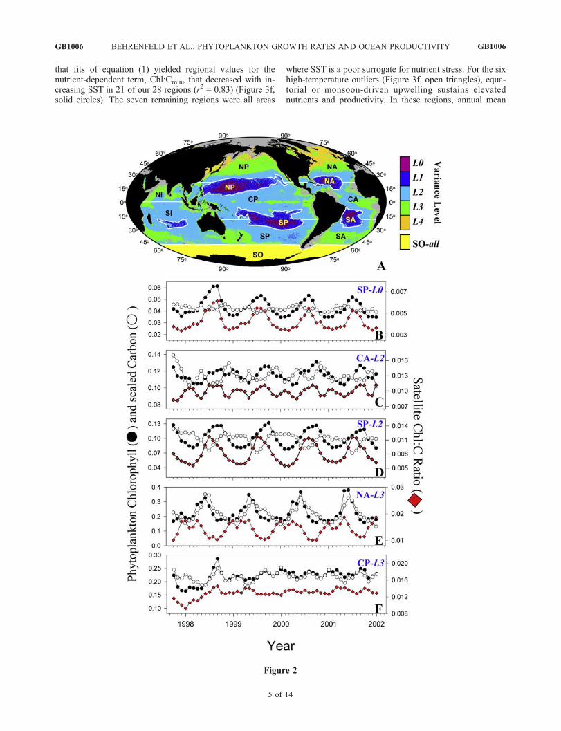
ocean circulation and ecosystem features. Parallel changesin Chl and C biomass reflect changes in phytoplanktonabundance caused by shifts in the balance betweenphytoplankton growth and losses (e.g., sinking, preda-tion). Divergent patterns in Chl and C (i.e., changes inthe Chl:C ratio) result from physiological acclimations tochanging growth conditions. Quite specifically, decreasesin Chl:C are associated with increases in growth irradi-ance (Ig), decreases in nutrients, and decreases in tem-perature [Geider, 1987; Sakshaug et al., 1989; Cloern etal., 1995; Geider et al., 1998; MacIntyre et al., 2002;Behrenfeld et al., 2002].[16] From our 28 regions, five basic seasonal patterns

emerged (Figure 2) (see the REGPAT figures in the auxil-iary material1 for all 28 regional graphs). In eight of thelowest production regions (see Figure 2 caption), stableenvironmental conditions foster stable C concentrationsthrough a tight coupling between phytoplankton growthand consumption, while seasonal changes in light causesmooth seasonal cycles in Chl, and thus Chl:C (Figure 2b).In other words, phytoplankton biomass is essentially con-stant throughout the year in these unproductive waters,but chlorophyll still varies notably from physiologicalresponses to seasonally changing growth conditions (i.e.,intracellular chlorophyll increases during winter months inresponse to generally deeper mixed layers, lower lightlevels, and possibly higher nutrient levels [Winn et al.,1995; McClain et al., 2004]). In four other low productionregions, the coupling between phytoplankton growth andconsumption is not so tight, and this imbalance causesmoderate changes in C and Chl biomass (Figure 2c).Physiological responses to changing light and nutrient stressin these regions cause additional variability in Chl that leadsto somewhat dampened Chl:C cycles with both spring andfall peaks (Figure 2c). Together, these 12 regions contributemost of the Chl-bbp pairs in Figure 1 at <0.14 mg Chl m�3,where chlorophyll variability is predominantly due tochanges in physiological state.[17] In five moderately productive regions, temporally

offset seasonal cycles of Chl and C biomass are found, withthe rise in Chl preceding the rise in C (Figure 2d). Weinterpret this pattern as a seasonal cycle where initial cell‘‘greening’’ is followed by increased growth and biomass,and later culminates in nutrient- and light-dependent reduc-tions in pigmentation and growth. Nine other moderate- andhigh-production areas exhibit seasonal cycles in both Chland C biomass that are dominated by large spring-summerblooms in phytoplankton abundance (Figure 2e). Despitethis first-order influence of biomass, physiological adjust-ments during the seasonal cycle are still registered bycoherent second-order changes in Chl:C ratios that in-crease during low-light and early bloom conditions anddecrease just prior to the biomass peak and crash(Figure 2e). These qualitative results thus indicate thatscatter in the Chl-bbp relationship at >0.14 mg Chl m�3

(Figure 1) is indeed associated with seasonal changes inphytoplankton physiology.

[18] The fifth temporal pattern revealed by this analysiswas unique to the two equatorial upwelling regions of thecentral Pacific (i.e., CP-L2, CP-L3 (Figure 2a)) andcharacterized by a strong shift in Chl:C during the1997–1998 El Nino to La Nina transition [Chavez et al.,1999; Behrenfeld et al., 2001], followed by an extendedperiod of low-level, correlated variability in Chl and C(Figure 2f ). This pattern is consistent with the regions’low amplitude variability in mixing depths and surfacelight (therefore, Ig) and the dominating influence of ElNino-La Nina shifts in nutrient availability on phytoplank-ton physiology (Figure 2f ).

3.3. Satellite-Derived Physiology Registers Light,Nutrient, and Temperature Effects

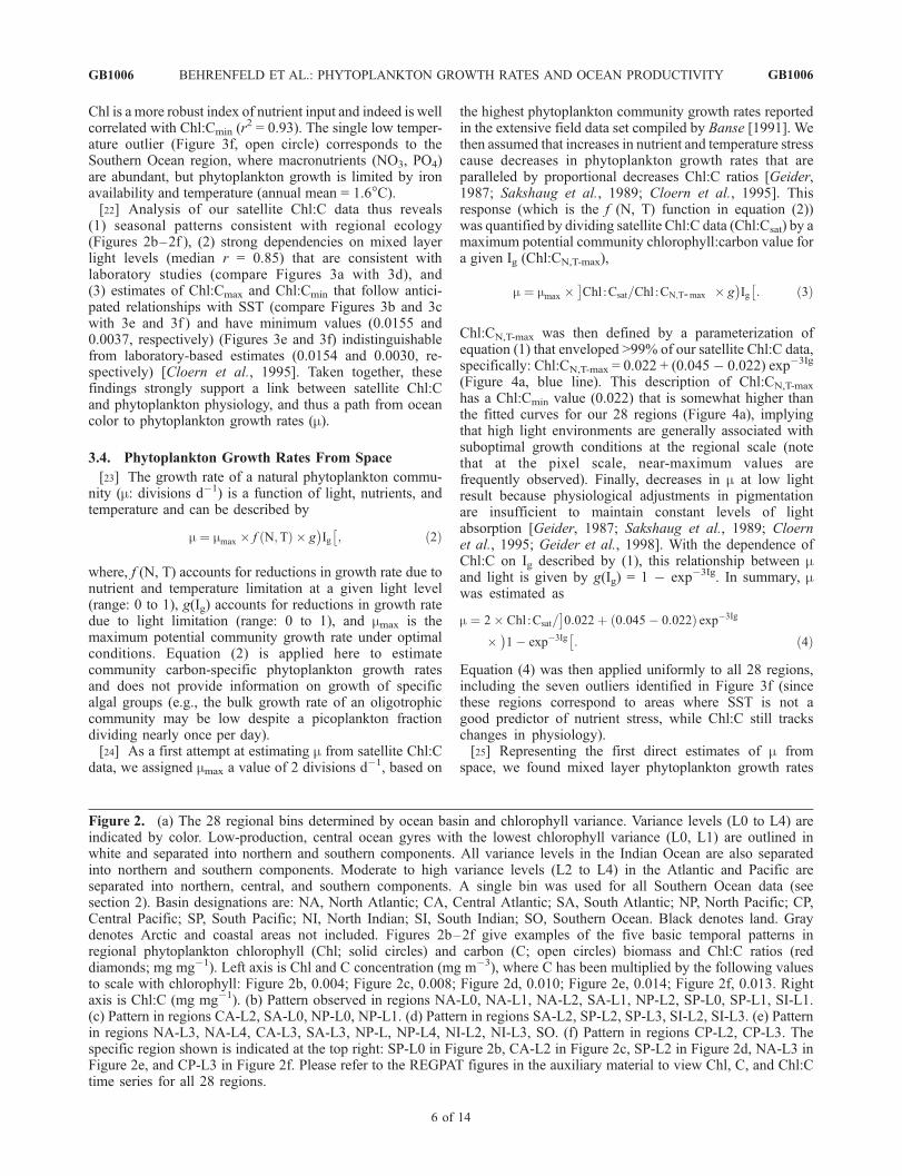
[19] It is well established from decades of laboratorystudies that phytoplankton Chl:C ratios decrease from lowto high light [e.g., Geider, 1987; Sakshaug et al., 1989;Geider et al., 1998; MacIntyre et al., 2002; Behrenfeld etal., 2002]. This phenomenon, known as ‘‘photoacclima-tion,’’ reflects physiological responses aimed at minimizingthe influence of light variability on growth (Figure 3a). Therelationship between Chl:C and light has a low-light max-imum (Chl:Cmax) that increases with increasing temperature[Geider, 1987; Cloern et al., 1995] (Figure 3b) and a light-saturated minimum (Chl:Cmin) that decreases with increas-ing nutrient stress [Laws and Bannister, 1980; Sakshaug etal., 1989; Cloern et al., 1995; Geider et al., 1998](Figure 3c). These adjustments in cellular pigmentationfunction to balance light harvesting with temperature- andnutrient-dependent changes in growth. The dependency ofChl:C on light can be modeled for a range of growthconditions as an exponential function of light [Cloern etal., 1995; Behrenfeld et al., 2002], such as

Chl : C ¼ Chl : Cmin þ Chl : Cmax � Chl : Cmin½ � exp�3 Ig : ð1Þ

[20] To more quantitatively link satellite Chl:C data withphytoplankton physiology, we compared regional changesin Chl:C with corresponding changes in mixed layer lightlevels (Ig) and found clear relationships that closely fol-lowed equation (1) (median r = 0.85) in all regions withsignificant seasonal variability in Ig (Figure 3d) (Table 1). Inother words, regional Chl:C values varied with Ig preciselyas expected from the laboratory (compare Figures 3a and3d). Overall, equation (1) captured 94% of the globalvariability in satellite Chl:C. Moreover, fits of equation(1) to the regional Chl:C data yielded Chl:Cmax values thatincreased with increasing sea surface temperature (SST)(r2 = 0.79) in a manner consistent with laboratory trends[Geider, 1987; Cloern et al., 1995] (Figure 3e). Differencesof scale in these relationships indicate that the nutrient-saturated, exponential growth conditions used in laboratorymonoculture studies (Figures 3a and 3b) are rarely replicatedfor all members of any natural phytoplankton community(Figures 3d and 3e).[21] While nutrient concentrations are not directly mea-

sured from space, the global tendency is for surfacenutrients to decrease with increasing SST [Kamykowskiet al., 2002; Switzer et al., 2003]. Accordingly, we found

1Auxiliary material is available at ftp://ftp.agu.org/apend/gb/2004GB002299.

GB1006 BEHRENFELD ET AL.: PHYTOPLANKTON GROWTH RATES AND OCEAN PRODUCTIVITY

4 of 14

GB1006

that fits of equation (1) yielded regional values for thenutrient-dependent term, Chl:Cmin, that decreased with in-creasing SST in 21 of our 28 regions (r2 = 0.83) (Figure 3f,solid circles). The seven remaining regions were all areas

where SST is a poor surrogate for nutrient stress. For the sixhigh-temperature outliers (Figure 3f, open triangles), equa-torial or monsoon-driven upwelling sustains elevatednutrients and productivity. In these regions, annual mean

Figure 2

GB1006 BEHRENFELD ET AL.: PHYTOPLANKTON GROWTH RATES AND OCEAN PRODUCTIVITY

5 of 14

GB1006

Chl is a more robust index of nutrient input and indeed is wellcorrelated with Chl:Cmin (r

2 = 0.93). The single low temper-ature outlier (Figure 3f, open circle) corresponds to theSouthern Ocean region, where macronutrients (NO3, PO4)are abundant, but phytoplankton growth is limited by ironavailability and temperature (annual mean = 1.6�C).[22] Analysis of our satellite Chl:C data thus reveals

(1) seasonal patterns consistent with regional ecology(Figures 2b–2f ), (2) strong dependencies on mixed layerlight levels (median r = 0.85) that are consistent withlaboratory studies (compare Figures 3a with 3d), and(3) estimates of Chl:Cmax and Chl:Cmin that follow antici-pated relationships with SST (compare Figures 3b and 3cwith 3e and 3f ) and have minimum values (0.0155 and0.0037, respectively) (Figures 3e and 3f) indistinguishablefrom laboratory-based estimates (0.0154 and 0.0030, re-spectively) [Cloern et al., 1995]. Taken together, thesefindings strongly support a link between satellite Chl:Cand phytoplankton physiology, and thus a path from oceancolor to phytoplankton growth rates (m).

3.4. Phytoplankton Growth Rates From Space

[23] The growth rate of a natural phytoplankton commu-nity (m: divisions d�1) is a function of light, nutrients, andtemperature and can be described by

m ¼ mmax � f N;Tð Þ � g Ig� �

; ð2Þ

where, f (N, T) accounts for reductions in growth rate due tonutrient and temperature limitation at a given light level(range: 0 to 1), g(Ig) accounts for reductions in growth ratedue to light limitation (range: 0 to 1), and mmax is themaximum potential community growth rate under optimalconditions. Equation (2) is applied here to estimatecommunity carbon-specific phytoplankton growth ratesand does not provide information on growth of specificalgal groups (e.g., the bulk growth rate of an oligotrophiccommunity may be low despite a picoplankton fractiondividing nearly once per day).[24] As a first attempt at estimating m from satellite Chl:C

data, we assigned mmax a value of 2 divisions d�1, based on

the highest phytoplankton community growth rates reportedin the extensive field data set compiled by Banse [1991]. Wethen assumed that increases in nutrient and temperature stresscause decreases in phytoplankton growth rates that areparalleled by proportional decreases Chl:C ratios [Geider,1987; Sakshaug et al., 1989; Cloern et al., 1995]. Thisresponse (which is the f (N, T) function in equation (2))was quantified by dividing satellite Chl:C data (Chl:Csat) by amaximum potential community chlorophyll:carbon value fora given Ig (Chl:CN,T-max),

m ¼ mmax � Chl :Csat=Chl :CN;T-max

� �� g Ig

� �: ð3Þ

Chl:CN,T-max was then defined by a parameterization ofequation (1) that enveloped >99% of our satellite Chl:C data,specifically: Chl:CN,T-max = 0.022 + (0.045� 0.022) exp�3Ig

(Figure 4a, blue line). This description of Chl:CN,T-max

has a Chl:Cmin value (0.022) that is somewhat higher thanthe fitted curves for our 28 regions (Figure 4a), implyingthat high light environments are generally associated withsuboptimal growth conditions at the regional scale (notethat at the pixel scale, near-maximum values arefrequently observed). Finally, decreases in m at low lightresult because physiological adjustments in pigmentationare insufficient to maintain constant levels of lightabsorption [Geider, 1987; Sakshaug et al., 1989; Cloernet al., 1995; Geider et al., 1998]. With the dependence ofChl:C on Ig described by (1), this relationship between mand light is given by g(Ig) = 1 � exp�3Ig. In summary, mwas estimated as

m ¼ 2� Chl :Csat= 0:022þ 0:045� 0:022ð Þ exp�3Ig� �

� 1� exp�3Ig� �

: ð4Þ

Equation (4) was then applied uniformly to all 28 regions,including the seven outliers identified in Figure 3f (sincethese regions correspond to areas where SST is not agood predictor of nutrient stress, while Chl:C still trackschanges in physiology).[25] Representing the first direct estimates of m from

space, we found mixed layer phytoplankton growth rates

Figure 2. (a) The 28 regional bins determined by ocean basin and chlorophyll variance. Variance levels (L0 to L4) areindicated by color. Low-production, central ocean gyres with the lowest chlorophyll variance (L0, L1) are outlined inwhite and separated into northern and southern components. All variance levels in the Indian Ocean are also separatedinto northern and southern components. Moderate to high variance levels (L2 to L4) in the Atlantic and Pacific areseparated into northern, central, and southern components. A single bin was used for all Southern Ocean data (seesection 2). Basin designations are: NA, North Atlantic; CA, Central Atlantic; SA, South Atlantic; NP, North Pacific; CP,Central Pacific; SP, South Pacific; NI, North Indian; SI, South Indian; SO, Southern Ocean. Black denotes land. Graydenotes Arctic and coastal areas not included. Figures 2b–2f give examples of the five basic temporal patterns inregional phytoplankton chlorophyll (Chl; solid circles) and carbon (C; open circles) biomass and Chl:C ratios (reddiamonds; mg mg�1). Left axis is Chl and C concentration (mg m�3), where C has been multiplied by the following valuesto scale with chlorophyll: Figure 2b, 0.004; Figure 2c, 0.008; Figure 2d, 0.010; Figure 2e, 0.014; Figure 2f, 0.013. Rightaxis is Chl:C (mg mg�1). (b) Pattern observed in regions NA-L0, NA-L1, NA-L2, SA-L1, NP-L2, SP-L0, SP-L1, SI-L1.(c) Pattern in regions CA-L2, SA-L0, NP-L0, NP-L1. (d) Pattern in regions SA-L2, SP-L2, SP-L3, SI-L2, SI-L3. (e) Patternin regions NA-L3, NA-L4, CA-L3, SA-L3, NP-L, NP-L4, NI-L2, NI-L3, SO. (f) Pattern in regions CP-L2, CP-L3. Thespecific region shown is indicated at the top right: SP-L0 in Figure 2b, CA-L2 in Figure 2c, SP-L2 in Figure 2d, NA-L3 inFigure 2e, and CP-L3 in Figure 2f. Please refer to the REGPAT figures in the auxiliary material to view Chl, C, and Chl:Ctime series for all 28 regions.

GB1006 BEHRENFELD ET AL.: PHYTOPLANKTON GROWTH RATES AND OCEAN PRODUCTIVITY

6 of 14

GB1006

Figure 3. Changes in phytoplankton Chl:C ratios in response to changes in light, nutrients, andtemperature as (Figures 3a–3c) observed in the laboratory and (Figures 3d–3f ) derived from satelliteocean color data. (a) Chl:C values measured in monocultures of the marine chlorophyte, Dunaliellatertiolecta, grown over a range of light levels (Ig) at 20�C and with replete nutrients. (b) Temperaturedependence of Chl:Cmax for 16 cultured phytoplankton species as reported by Geider [1987]. Solidcircles denote diatoms. Open circles denote all other species. (c) Influence of nutrient stress on Chl:Cmin

in the diatom, Thalassiosira fluviatilis [Laws and Bannister, 1980]. Nutrient stress is quantified bychanges in growth rate (x axis). Solid circles denote NO3 limited cultures. Open circles denote NH4

limited cultures. Solid triangles denote PO4 limited cultures. (d) Satellite Chl:C estimates versus Ig forfour of the regions defined in Figure 2a. Solid circles denote SP-L1. Solid diamonds denote NA-L2. Solidupside-down triangles denote SP-L2. Solid right-side-up triangles denote SA-L1. Fitted curves for all28 regions are shown in Figure 4a, and fit statistics are provided in Table 1. (e) Relationship between seasurface temperature (SST: �C) and fitted values of Chl:Cmax for all 28 regions. Solid line denotes fit todata (Chl:Cmax = 0.0155 + 0.00005 exp 0.215 SST) (r2 = 0.79). (f ) Relationship between sea surfacetemperature (SST: �C) and fitted values of Chl:Cmin for all 28 regions. Solid line denotes fit to solid circledata (Chl:Cmin = 0.017 � 0.00045 SST) (r2 = 0.83). Open triangles denote the six high-temperatureoutliers (L2 and L3 data from the North Indian, Central Pacific, Central Atlantic). Open circle denoteslow-temperature outlier (Southern Ocean). These ‘‘outliers’’ are anticipated based on regionalrelationships between SST and constraints on phytoplankton growth (see text). Solid line in Figures3a and 3d denotes fit of (1). Solid line in Figure 3b denotes fit of exponential model as in Figure 3e. Solidline in Figure 3c denotes linear regression fit to all data.

GB1006 BEHRENFELD ET AL.: PHYTOPLANKTON GROWTH RATES AND OCEAN PRODUCTIVITY

7 of 14

GB1006

to be persistently elevated in the upwelling-enrichedtropical oceans, chronically suppressed in the stratifiedcentral ocean gyres, and strongly seasonal at highernorthern and southern latitudes (Figures 4b and 4c). Inthe equatorial Pacific, m peaked along the upwelling axisnear the equator and then diminished to the northand south (Figures 4b and 4c), as often suggested byfield 14C-uptake measurements [Lindley et al., 1995;Behrenfeld and Boss, 2003]. At high southern latitudeswhere easterly circumpolar currents prevail, enhancedsummertime growth rates were largely restricted to theleeward eastern margins of continents and islands(Figure 4c), consistent with sources of growth-limitingmicronutrients (i.e., iron) [Boyd et al., 1999; Sullivan et al.,1993]. In the North Atlantic and western Pacific, spring andsummer growth rates were broadly elevated across middleand high latitudes, reflecting a shoaling of surface mixing

depths and elevated sunlight (Figure 4b). The markedlylower summer growth rates in the eastern subarctic Pacificare consistent with this region’s restriction by iron availabil-ity [Boyd et al., 1996; Harrison et al., 1999] (Figure 4b).Globally, satellite-based phytoplankton community growthrates exhibited a smooth, peaked distribution with a medianaround 0.5 divisions d�1 (Figure 4d).

3.5. Global Ocean Productivity

[26] The product of phytoplankton carbon biomass andgrowth rate is net primary production. Water column NPPcan be estimated from surface satellite C and m by addi-tionally accounting for changes in photosynthesis withdepth,

NPP ¼ C� m� Zeu � h I0ð Þ; ð5Þ

Table 1. Mean Surface Chlorophyll Biomass (mg m�3), Mean Sea Surface Temperature (SST: �C), and Range in Median Mixed Layer

Light Levels (Ig: Moles Photons m�2 h�1) for Each Region (See Figure 2) During the September 1997 to January 2002 Perioda

Region Mean Chl Biomass Mean SST Ig Min–Max Chl:Cmin Chl:Cmax Correlation Coefficients

North AtlanticL0 0.053 26 0.85–2.51 0.0044 0.025 0.90L1 0.060 26 0.82–2.3 0.0049 0.028 0.85L2 0.091 23 0.26–2.67 0.0058 0.021 0.89L3 0.226 16 0.01–1.61 0.0112 0.017 0.91L4 0.413 8 <0.01–0.70 0.0133 0.016 0.65

Central AtlanticL2 0.115 26 1.28–1.59 0.0095 0.027 0.67L3 0.180 25 1.32–1.80 0.0115 0.027 0.72

South AtlanticL0 0.054 25 0.73–2.30 0.0046 0.017 0.87L1 0.063 24 0.74–2.60 0.0054 0.024 0.91L2 0.113 18 0.20–1.91 0.0073 0.017 0.89L3 0.254 12 0.04–0.74 0.0120 0.016 0.68

North PacificL0 0.060 27 1.09–1.67 0.0053 0.031 n.s.L1 0.071 26 0.97–1.85 0.0063 0.028 0.48L2 0.091 22 0.37–2.61 0.0077 0.022 0.91L3 0.219 13 0.01–1.91 0.0110 0.016 0.67L4 0.411 9 <0.01–0.37 0.0120 0.015 n.s.

Central PacificL2 0.130 27 1.10–1.50 0.0110 0.031 n.s.L3 0.220 27 1.33–1.88 0.0130 0.028 n.s.

South PacificL0 0.043 24 0.68–2.38 0.0037 0.016 0.90L1 0.072 24 0.67–1.98 0.0060 0.017 0.95L2 0.101 16 0.27–1.94 0.0061 0.019 0.96L3 0.213 14 0.09–1.37 0.0100 0.020 0.85

North IndianL2 0.141 22 1.18–1.96 0.0135 0.037 0.67L3 0.219 29 0.59–2.01 0.0140 0.045 0.94

South IndianL1 0.061 28 0.62–2.60 0.0049 0.020 0.85L2 0.128 21 0.32–1.90 0.0083 0.019 0.83L3 0.211 17 0.09–1.19 0.0101 0.015 0.85

Southern OceanAll 0.168 2 0.01–0.60 0.004 0.013 0.81

aAlso provided is Chl:Cmin, Chl:Cmax, and correlation coefficients for regional fits of equation (1). Chl:Cmin and Chl:Cmax [mg Chl (mg C)�1] are allsignificant at p < 0.0005; n.s. = not significant.

GB1006 BEHRENFELD ET AL.: PHYTOPLANKTON GROWTH RATES AND OCEAN PRODUCTIVITY

8 of 14

GB1006

where Zeu is the depth (m) of the photosynthetically activesurface layer and h(I0) describes how changes in surfacelight influence the depth-dependent profile of carbonfixation. Equation (5) is of the same form as earlier NPPmodels [Behrenfeld and Falkowski, 1997b], with theexception that Chl is replaced by C and the empiricalestimate of chlorophyll-specific photosynthesis (Popt

b ) isreplaced by m (where C and m are now directly estimatedfrom remote sensing; see above). To illustrate the impact ofthis new carbon-based approach, we now compare NPPcalculated from (5) and a common Chl-based algorithm,the Vertically Generalized Production Model (VGPM)[Behrenfeld and Falkowski, 1997a] (see section 2.4).[27] Annual total global ocean productivity averaged

67 Pg C yr�1 (Pg = 1015 g) for the C-based model and60 Pg C yr�1 for the Chl-based model over the 1997 to 2002period, a difference that scales directly with the value ofmmax. Far more striking (and independent of mmax) are thespatial and seasonal differences in NPP between models(Figures 5a–5d). The carbon model yielded 40% and 49%higher annual NPP for the central Atlantic and centralPacific regions (see Figure 2 for regional boundaries) andan increase from 1.6 to 2.6 Pg C yr�1 in the north Indian

region (Figures 5e and 5f ). (It is interesting to note that thetwo models are in better agreement in these areas when anexponential model for Popt

b , following Antoine et al. [1996],is used in the VGPM. This exponential expression performsbetter at low latitudes than the standard VGPM model basedon comparisons with 14C data [Campbell et al., 2002].)Carbon-based NPP was also higher by 9% in the southIndian, 7% in the North Pacific, and 2% in the South Pacificregions (Figures 5e and 5f ). The opposite trend was foundfor the North and South Atlantic, where NPP was 21% and18% lower for the C model than the Chl model, respectively(Figures 5e and 5f ). In the Southern Ocean, the relationshipbetween C- and Chl-based NPP was patchy (particularly insummer months) (Figure 5f ), but overall the C model gavea 20% lower estimate for this region.[28] Without exception, the C-based and Chl-based

models yielded different seasonal cycles in NPP, andoften dramatically so (see the NPP figures in the auxiliarymaterial to view time series for all 28 regions). Whileeach region exhibited unique differences, the generaltrend over variance levels was for the C model to givedampened cycles relative to the Chl model in lowvariance regions, and often stronger and delayed seasonal

Figure 4. (a) Phytoplankton chlorophyll to carbon (Chl:C) ratios versus median mixed layer growthirradiance (Ig: moles photons m�2 h�1). Blue line denotes modeled maximum Chl:C. Gray lines denotefits of (1) to the 28 regions (see Figure 2a). Figures 4b and 4c show seasonal mean mixed layerphytoplankton growth rates (m: divisions d�1) calculated from satellite Chl:C using (2). (b) Borealsummer (June to August). (c) Boreal winter (December to February). (d) Frequency histogram of annualmean satellite-based phytoplankton growth rates.

GB1006 BEHRENFELD ET AL.: PHYTOPLANKTON GROWTH RATES AND OCEAN PRODUCTIVITY

9 of 14

GB1006

cycles in higher variance regions (see the NPP figures inthe auxiliary material).[29] When viewed by ocean basin (i.e., combining all

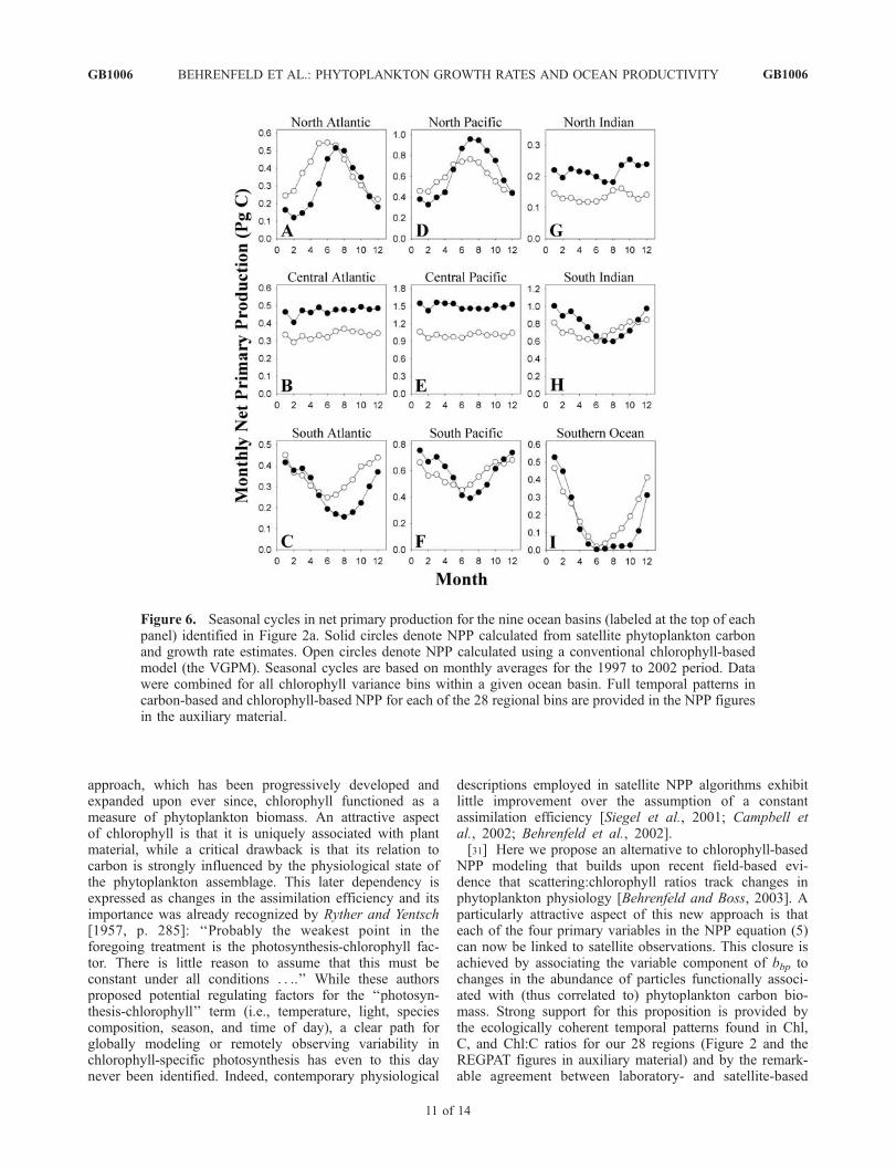
variance levels), the C model typically gave strongerseasonal cycles in NPP at high latitudes (Figures 6a, 6c,6d, and 6f ) and persistently higher NPP at tropical latitudes(Figures 6b, 6e, and 6g). For the North Indian region, the Cmodel indicated enhanced NPP (0.21–0.25 Pg C month�1)in the spring (March to late May) and fall (October–December), while the Chl model yielded only a single peak(0.16 Pg C month�1) between September and November(Figure 6g). Both models gave similar magnitude (0.8 to1.0 Pg C month�1), single-peaked annual cycles in NPP forthe South Indian region, but the C-based cycle was offsetlater by roughly 2 months (Figure 6h). The two models alsogave similar magnitude midsummer maxima in NPP (0.4 to0.5 Pg C month�1) and nearly identical fall declines for theNorth and South Atlantic, but summer highs for the C modelwere slower to develop and more sharply peaked than thebroad maxima given by the Chl model (Figures 6a and 6d).A similar delay in the time of the spring bloom was alsoindicated for the Southern Ocean by the C model (Figure 6i).

In contrast, timing of the seasonal cycle and annual inte-grated production were similar for the two models in theNorth Pacific, but the C model gave a 25% higher summerpeak (0.96 Pg C month�1) and 27% lower winter minimum(0.12 Pg C month�1) in NPP than the Chl model (Figure 6d).In all northern and southern regions of the Atlantic andPacific and in the Southern Ocean, the C-based model gavelower winter minima in NPP than the Chl-based model(Figures 6a, 6c, 6d, and 6f ).

4. Discussion

[30] Quantification of areal net primary production froma limited set of surface observations has been a long-standing quest that can arguably be said to have roots ina 1957 paper by John H. Ryther and Charles S. Yentsch[Ryther and Yentsch, 1957]. In that seminal contribution,NPP was related to the product of chlorophyll biomass,daily integrated surface solar radiation, an average extinc-tion coefficient for visible light in the water column, anda constant chlorophyll-specific assimilation efficiency of3.7 g C (g Chl h)�1 [Ryther and Yentsch, 1957]. In their

Figure 5. Seasonal mean water column net primary production (mg C m2 d�1) calculated from (a, b)satellite phytoplankton carbon and growth rate estimates and (c, d) a conventional chlorophyll-based model(the VGPM). The difference between these model NPP estimates (Figure 5e = Figure 5a – Figure 5c;Figure 5f = Figure 5b – Figure 5d) has significant implications on regional carbon cycling. (a, c, e) Borealsummer (June to August). (b, d, f ) Boreal winter (December to February).

GB1006 BEHRENFELD ET AL.: PHYTOPLANKTON GROWTH RATES AND OCEAN PRODUCTIVITY

10 of 14

GB1006

approach, which has been progressively developed andexpanded upon ever since, chlorophyll functioned as ameasure of phytoplankton biomass. An attractive aspectof chlorophyll is that it is uniquely associated with plantmaterial, while a critical drawback is that its relation tocarbon is strongly influenced by the physiological state ofthe phytoplankton assemblage. This later dependency isexpressed as changes in the assimilation efficiency and itsimportance was already recognized by Ryther and Yentsch[1957, p. 285]: ‘‘Probably the weakest point in theforegoing treatment is the photosynthesis-chlorophyll fac-tor. There is little reason to assume that this must beconstant under all conditions . . ..’’ While these authorsproposed potential regulating factors for the ‘‘photosyn-thesis-chlorophyll’’ term (i.e., temperature, light, speciescomposition, season, and time of day), a clear path forglobally modeling or remotely observing variability inchlorophyll-specific photosynthesis has even to this daynever been identified. Indeed, contemporary physiological

descriptions employed in satellite NPP algorithms exhibitlittle improvement over the assumption of a constantassimilation efficiency [Siegel et al., 2001; Campbell etal., 2002; Behrenfeld et al., 2002].[31] Here we propose an alternative to chlorophyll-based

NPP modeling that builds upon recent field-based evi-dence that scattering:chlorophyll ratios track changes inphytoplankton physiology [Behrenfeld and Boss, 2003]. Aparticularly attractive aspect of this new approach is thateach of the four primary variables in the NPP equation (5)can now be linked to satellite observations. This closure isachieved by associating the variable component of bbp tochanges in the abundance of particles functionally associ-ated with (thus correlated to) phytoplankton carbon bio-mass. Strong support for this proposition is provided bythe ecologically coherent temporal patterns found in Chl,C, and Chl:C ratios for our 28 regions (Figure 2 and theREGPAT figures in auxiliary material) and by the remark-able agreement between laboratory- and satellite-based

Figure 6. Seasonal cycles in net primary production for the nine ocean basins (labeled at the top of eachpanel) identified in Figure 2a. Solid circles denote NPP calculated from satellite phytoplankton carbonand growth rate estimates. Open circles denote NPP calculated using a conventional chlorophyll-basedmodel (the VGPM). Seasonal cycles are based on monthly averages for the 1997 to 2002 period. Datawere combined for all chlorophyll variance bins within a given ocean basin. Full temporal patterns incarbon-based and chlorophyll-based NPP for each of the 28 regional bins are provided in the NPP figuresin the auxiliary material.

GB1006 BEHRENFELD ET AL.: PHYTOPLANKTON GROWTH RATES AND OCEAN PRODUCTIVITY

11 of 14

GB1006

dependencies of Chl:C on light, temperature, and nutrientstress (Figure 3).[32] An important point emphasized by our results is that

chlorophyll concentration is a poor proxy of phytoplanktonbiomass within large areas of the ocean. Particularly in low-biomass oligotrophic regions, chlorophyll variability can bedominated by, if not exclusively due to, adjustments inphysiological state (i.e., changes in Chl:C resulting fromchanges in growth conditions). This decoupling betweenphytoplankton biomass and pigmentation has been indicatedin the vertical dimension of the water column [e.g., Kieferand Kremer, 1981;Kitchen and Zaneveld, 1990;Mitchell andKiefer, 1988; Mitchell and Holm-Hansen, 1991; Fennel andBoss, 2003] and here is simply extended on a global scale tothe horizontal dimension. In both the vertical and horizontaldimensions, however, the physiological underpinning for thisindependent behavior in carbon and chlorophyll biomass isthe same: acclimation to changing light, nutrient, and tem-perature conditions.[33] The link between satellite Chl:C and phytoplankton

physiology established here has benefited from a variety offactors. For example, excluding optically complex coastalregions and integrating open ocean data over large time(monthly) and space (regional) scales undoubtedly helpsremove local-scale variability in the bbp:C ratio. The widerange of growth conditions in the global oceans also helpscreate a dynamic range in Chl:C that is sufficient toovercome optically based changes in the bbp to phytoplank-ton C relationship. Perhaps the most important factor,though, is the apparent compositional stability of naturalparticle assemblages. Indeed, field studies suggest that overseasonal cycles [DuRand et al., 2001] and across oligotro-phic to eutrophic conditions [Oubelkheir, 2001] phytoplank-ton contribute a relatively consistent fraction to POC,although exceptions to this rule certainly exist. For theplanktonic contributors to bbp, this relationship may beparticularly tight because the rapid potential growth ratesof the heterotrophic component allow for a close correspon-dence between their biomass and phytoplankton abundance.[34] The quest to quantify areal net primary production

over regional to global scales is certainly not over yet, butour results suggest that an important step has been taken inthis direction. Already, the carbon-based approach hasrevealed some unexpected and fascinating temporal patternsin regional NPP (Figure 6, and the NPP figures in theauxiliary material) and raised important questions regardingthe functioning of planktonic communities. One particularlyintriguing observation has been the bilinear relationshipbetween Chl and bbp (Figure 1). This pattern suggests thatat least at the regional scale, a minimum exists to which theheterotrophic community is ‘‘willing’’ to graze the phyto-plankton [Lessard and Murrell, 1998]. Is there an energeticjustification for this apparent ‘‘floor’’ in phytoplanktonabundance? If not, what is the basis for this ‘‘hinge-point’’between physiologically dominated and biomass-dominatedsystems? Another interesting observation has been theorganization of regional Chl, C, and Chl:C data into fivebasic temporal patterns (Figure 2). Are these patterns simplydue to ocean circulation and other physical constraints, orare they also associated with dominant ecosystem modes?

Certainly, there is much left to be done here and much left tolearn.

4.1. Future Directions

[35] A multitude of future research needs and excitingpotential applications emerge with this first indication of aspace-based optical index of phytoplankton physiology.Clearly of foremost importance is the continued develop-ment and validation of derived satellite products, includingbbp, phytoplankton pigment and carbon biomass, m, andNPP. These developments will require new field measure-ments (as there is currently a paucity of such data) and anevolution in satellite ocean color technology that allowsbetter separation of optically active in-water constituents(e.g., utilizing ultraviolet wave bands to better separatephytoplankton and colored dissolved organic material ab-sorption) and improved atmospheric corrections (e.g., char-acterization of absorbing aerosol column thickness andheights).[36] Improvements in the carbon-based approach can also

be made in the many steps leading from satellite Chl and bbpto NPP. For example, in (3) we assume that nutrient-dependent changes in Chl:C are paralleled by equivalentchanges in m. However, laboratory studies indicate thatwhen m = 0 division d�1, Chl:C is > 0. In addition, we havenot yet considered potential taxonomic influences on therelationship between Chl:C and m, nor have we attempted toadjust the bbp to phytoplankton carbon relationship toaccount for changes in particle size distributions (oftenassociated with features such as high-latitude spring diatomblooms) or the occurrence of high concentrations of inor-ganic particles (e.g., coccoliths, suspended sediments). Cal-culations of NPP might also benefit from expanding thecurrent depth-integrated model (5) into a time-, depth-, andwavelength-resolved model. Relating m to phytoplanktonabsorption:C rather than Chl:C may also be worthwhile, asthe former is physiologically more relevant and absorption isoperationally closer to ocean color than chlorophyll. Alter-native relationships between Chl:C and m might additionallybe considered for physiologically unique growth conditions,such as in iron-limited high-nutrient, low-chlorophyll(HNLC) waters.[37] One of the simplifying assumptions in our current

estimates of m from Chl:C is that surface phytoplanktonassemblages are in a state of balanced growth; that is, allcellular constituents (particularly carbon and chlorophyll)are in a fully acclimated state (i.e., growing at the samerate). This assumption allows the use of basic physiologicalexpressions and may very well be valid for the large spatialand temporal scales considered here. However, when phys-ical perturbations to mixed layer growth conditions occur ontimescales similar to or shorter than timescales of acclima-tion, transient episodes of unbalanced growth can ensue.Under such conditions, relationships between Chl:C and mbecome complicated and can require more complex ‘‘dy-namic’’ physiological models [e.g., Geider et al., 1998;Flynn, 2001; Flynn et al., 2001] to unravel. This issue ofaccounting for balanced versus unbalanced growth will beone of the challenges faced in extending the carbon-basedapproach to smaller space (<1 km2) and time (daily) scales.

GB1006 BEHRENFELD ET AL.: PHYTOPLANKTON GROWTH RATES AND OCEAN PRODUCTIVITY

12 of 14

GB1006

[38] A potentially important application for our phyto-plankton carbon biomass and growth rate data, beyondquantifying ocean production and detecting its change,is for the development of prognostic ocean circulation-ecosystem models (i.e., ‘‘coupled models’’). In suchmodels, phytoplankton carbon (or nitrogen) biomass andgrowth rates are primary derived variables. In the past, noremote sensing data have been available to directly testmodeled growth rate fields, and broad assumptions havebeen necessary regarding Chl:C ratios (often assumedconstant) to compare modeled phytoplankton carbon bio-mass with satellite chlorophyll data. It will now bepossible with the new carbon-based approach to directlycompare satellite and model estimates of phytoplanktoncarbon biomass and growth rates.

4.2. Perspective

[39] Photosynthesis is the primary conduit through whichinorganic carbon enters the living components of thebiosphere. In addition to linking ecosystem and biogeo-chemical processes, terrestrial and ocean productivity isfunctionally dependent on climate and is thus an indicatorof temporal change in environmental forcings. Remotesensing is a route through which prohibitive space-timegaps in surface measurements of photosynthesis can beovercome; but photosynthesis is not directly amenable tosatellite detection. For the oceans, empirical conversionfactors employed to relate satellite data products (i.e.,chlorophyll) to production have entailed such large uncer-tainties that any hope of detecting global change has beencompromised.[40] Here we present a path for retrieving the ‘‘missing

piece’’ of the productivity equation from space. Our ap-proach is rooted in well-developed physiological dependen-cies on light, nutrients, and temperature and in a solidunderstanding of the light scattering and absorption prop-erties of ocean waters. Our resultant carbon-based NPPestimates provide a dramatically different view of howocean productivity is distributed over space and time andpoint to the importance of this new development. Withfuture improvements in ocean color remote sensing (i.e.,expanded wave bands, improved atmospheric corrections)and algorithm development, the full potential of this carbon-based approach will be realized and, through the resultantclosure on the productivity equation, NPP estimates will beachieved with higher fidelity and an improved capacity fordetecting real trends in global ocean carbon cycling.

[41] Acknowledgments. This research was supported by the NationalAeronautics and Space Administration (RTOP622-52-58, NAS5-00196,NAS5-00200, NAG5-12400) and the National Science Foundation (NSF-INT99-02240, OCE-0241614). We thank Karl Banse, Phil Boyd, andVanessa Sherlock for very helpful comments and discussions, StephaneMaritorena for remote sensing data, and Elizabeth Tollefson for support.

ReferencesAntoine, D., J.-M. Andre, and A. Morel (1996), Oceanic primary produc-tion: 2. Estimation at global scale from satellite (coastal zone color scan-ner) chlorophyll, Global Biogeochem. Cycles, 10, 57–69.

Babin, M., A. Morel, V. Fournier-Sicre, F. Fell, and D. Stramski (2003),Light scattering properties of marine particles in coastal and open oceanwaters as related to the particle mass concentration, Limnol. Oceanogr.,48, 843–859.

Bader, H. (1970), The hyperbolic distribution of particle sizes, J. Geophys.Res., 75, 2822–2830.

Banse, K. (1991), Rates of phytoplankton cell division in the field and iniron enrichment experiments, Limnol. Oceanogr., 36, 1886–1898.

Behrenfeld, M. J., and E. Boss (2003), The beam attenuation to chlorophyllratio: An optical index of phytoplankton physiology in the surfaceocean?, Deep Sea Res., Part I, 50, 1537–1549.

Behrenfeld, M. J., and P. G. Falkowski (1997a), Photosynthetic rates de-rived from satellite-based chlorophyll concentration, Limnol. Oceanogr.,42, 1–20.

Behrenfeld, M. J., and P. G. Falkowski (1997b), A consumer’s guide tophytoplankton primary productivity models, Limnol. Oceanogr., 42,1479–1491.

Behrenfeld, M. J., et al. (2001), Biospheric primary production during anENSO transition, Science, 291, 2594–2597.

Behrenfeld, M. J., E. Maranon, D. A. Siegel, and S. B. Hooker (2002),A photoacclimation and nutrient based model of light-saturated photo-synthesis for quantifying oceanic primary production, Mar. Ecol. Prog.Ser., 228, 103–117.

Bishop, J. K. B. (1999), Transmissometer measurements of POC, Deep SeaRes., Part I, 46, 353–369.

Bishop, J. K. B., S. E. Calvert, and M. Y. S. Soon (1999), Spatial andtemporal variability of POC in the northeast Subarctic Pacific, DeepSea Res., Part II, 46, 2699–2733.

Boyd, P. W., et al. (1996), In vitro iron enrichment experiments in the NESubarctic Pacific, Mar. Ecol. Prog. Ser., 136, 179–196.

Boyd, P., J. LaRoche, M. Gall, R. Frew, and R. M. L. McKay (1999),The role of iron, light, and silicate in controlling algal biomass in sub-Antarctic waters southeast of New Zealand, J. Geophys. Res., 104,13,395–13,404.

Campbell, J., et al. (2002), Comparison of algorithms for estimating pri-mary productivity from surface chlorophyll, temperature and irradiance,Global Biogeochem. Cycles, 16(3), 1035, doi:10.1029/2001GB001444.

Chavez, F. P., et al. (1999), Biological and chemical response of theequatorial Pacific Ocean to the 1997–98 El Nino, Science, 286,2126–2131.

Cho, B. C., and F. Azam (1990), Biogeochemical significance of bacterialbiomass in the ocean’s euphotic zone, Mar. Ecol. Prog. Ser., 63, 253–259.

Claustre, H., A. Morel, M. Babin, C. Cailliau, D. Marie, J.-C. Marty,D. Tailliez, and D. Vaulot (1999), Variability in particle attenuation andchlorophyll fluorescence in the tropical Pacific: Scales, patterns, andbiogeochemical implications, J. Geophys. Res., 104, 3401–3422.

Cloern, J. E., C. Grenz, and L. Vidergar-Lucas (1995), An empirical modelof the phytoplankton chlorophyll/carbon ratio—The conversion factorbetween productivity and growth rate, Limnol. Oceanogr., 40, 1313–1321.

Doney, S. C., D. M. Glover, S. J. McCue, and F. Montserrat (2003), Me-soscale variability of Sea-viewing Wide Field-of-view Sensor (SeaWiFS)satellite ocean color: Global patterns and spatial scales, J. Geophys. Res.,108(C2), 3024, doi:10.1029/2001JC000843.

DuRand, M. D., R. J. Olson, and S. W. Chisholm (2001), Phytoplanktonpopulation dynamics at the Bermuda Atlantic Time-series station in theSargasso Sea, Deep Sea Res., Part II, 48, 1983–2003.

Eppley, R. W., F. P. Chavez, and R. T. Barber (1992), Standing stocks ofparticulate carbon and nitrogen in the equatorial Pacific at 150�W,J. Geophys. Res., 97, 655–661.

Esaias, W. E., R. L. Iverson, and K. Turpie (1999), Ocean province classi-fication using ocean colour data: Observing biological signatures of var-iations in physical dynamics, Global Change Biol., 6, 39–55.

Fennel, K., and E. Boss (2003), Subsurface maxima of phytoplankton andchlorophyll: Steady state solutions from a simple model, Limnol. Ocean-ogr., 48, 1521–1534.

Flynn, K. J. (2001), A mechanistic model for describing dynamic multi-nutrient, light, temperature interactions in phytoplankton, J. PlanktonRes., 23, 977–997.

Flynn, K. J., H. Marshall, and R. J. Geider (2001), A comparison of twoN-irradiance interaction models of phytoplankton growth, Limnol.Oceanogr., 46, 1794–1802.

Gardner, W. D., I. D. Walsh, and M. J. Richardson (1993), Biophysicalforcing on particle production and distribution during a spring bloom inthe North Atlantic, Deep Sea Res., Part II, 40, 171–195.

Gardner, W. D., S. P. Chung, M. J. Richardson, and I. D. Walsh (1995), Theoceanic mixed-layer pump, Deep Sea Res., Part II, 42, 757–775.

Garver, S. A., and D. A. Siegel (1997), Inherent optical property inver-sion of ocean color spectra and its biogeochemical interpretation: I.Time series from the Sargasso Sea, J. Geophys. Res., 102, 18,607–18,625.

GB1006 BEHRENFELD ET AL.: PHYTOPLANKTON GROWTH RATES AND OCEAN PRODUCTIVITY

13 of 14

GB1006

Geider, R. J. (1987), Light and temperature dependence of the carbon tochlorophyll ratio in microalgae and cyanobacteria: Implications for phys-iology and growth of phytoplankton, New Phytol., 106, 1–34.

Geider, R. J., H. L. MacIntyre, and T. Kana (1998), A dynamic regulatorymodel of phytoplanktonic acclimation to light, nutrients, and temperature,Limnol. Oceanogr., 43, 679–694.

Gundersen, K., K. M. Orcutt, D. A. Purdie, A. F. Michaels, and A. H. Knap(2001), Particulate organic carbon mass distribution at the BermudaAtlantic time-series Study (BATS) site, Deep Sea Res., Part II, 48,1697–1718.

Harrison, P. J., et al. (1999), Comparison of factors controlling phytoplank-ton productivity in the NE and NW subarctic Pacific, Prog. Oceanogr.,43, 205–234.

Kamykowski, D., S.-J. Zentara, J. M. Morrison, and A. C. Switzer (2002),Dynamic global patterns of nitrate, phosphate, silicate, and iron avail-ability and phytoplankton community composition from remote sensingdata, Global Biogeochem. Cycles , 16(4), 1077, doi:10.1029/2001GB001640.

Kiefer, D. A., and J. Berwald (1992), A random encounter model for themicrobial planktonic community, Limnol. Oceanogr., 37, 457–467.

Kiefer, D. A., and J. N. Kremer (1981), Origins of the vertical patterns ofphytoplankton and nutrients in the temperate, open ocean: A stratigraphichypothesis, Deep Sea Res., 28, 1087–1105.

Kitchen, J., and J. R. Zaneveld (1990), On the noncorrelation of the verticalstructure of light scattering and chlorophyll a in case I waters, J. Geo-phys. Res., 95, 20,237–20,246.

Laws, E. A., and T. T. Bannister (1980), Nutrient- and light-limitedgrowth of Thalassiosira fluviatilis in continuous culture, with implica-tions for phytoplankton growth in the ocean, Limnol. Oceanogr., 25,457–473.

Lessard, E. J., and M. C. Murrell (1998), Microzooplankton herbivory andphytoplankton growth in the northwestern Sargasso Sea, Aquat. Micro-bial Ecol., 16, 173–188.

Lindley, S. T., R. R. Bidigare, and R. T. Barber (1995), Phytoplanktonphotosynthesis parameters along 140�W in the equatorial Pacific, DeepSea Res., Part II, 42, 441–463.

Loisel, H., and A. Morel (1998), Light scattering and chlorophyll concen-tration in case 1 waters: A reexamination, Limnol. Oceanogr., 43, 847–858.

Loisel, H., E. Bosc, D. Stramski, K. Oubelkheir, and P.-Y. Deschamps(2001), Seasonal variability of the backscattering coefficient in the Med-iterranean Sea on Satellite SeaWiFS imagery, Geophys. Res. Lett., 28,4203–4206.

Longhurst, A. (1995), Seasonal cycles of pelagic production and consump-tion, Prog. Oceanogr., 36, 77–167.

MacIntyre, H. L., T. M. Kana, T. Anning, and R. J. Geider (2002),Photoacclimation of photosynthesis irradiance response curves andphotosynthetic pigments in microalgae and cyanobacteria, J. Phycol.,38, 17–38.

Maritorena, S., D. A. Siegel, and A. R. Peterson (2002), Optimization of asemianalytical ocean color model for global-scale applications, Appl.Opt., 41, 2705–2714.

McClain, C. R., S. R. Signorini, and J. R. Christian (2004), Subtropicalgyre variability observed by ocean-color satellites, Deep Sea Res., Part II,51, 281–301.

Mitchell, B. G., and O. Holm-Hansen (1991), Bio-optical properties ofAntarctic Peninsula waters: Differentiation from temperate ocean models,Deep Sea Res., 38, 1009–1028.

Mitchell, B. G., and D. A. Kiefer (1988), Variability in pigment specificparticulate fluorescence and absorption spectra in the northeastern PacificOcean, Deep Sea Res., 35, 665–689.

Morel, A., and Y.-H. Ahn (1991), Optics of heterotrophic nanoflagellates andciliates: A tentative assessment of their scattering role in oceanic waterscompared to those of bacterial and algal cells, J. Mar. Res., 48, 1–26.

Oubelkheir, K. (2001), Biogeochemical characterization of various oceanicprovinces through optical indicators over various space and time scales,Ph.D. thesis, 216 pp., Univ. de la Mediter./CNRS, Marseille, France.

Ryther, J. H., and C. S. Yentsch (1957), The estimation of phytoplanktonproduction in the ocean from chlorophyll and light data, Limnol. Ocean-ogr., 2, 281–286.

Sakshaug, E., K. Andresen, and D. A. Kiefer (1989), A steady state de-scription of growth and light absorption in the marine planktonic diatomSkeletonema costatum, Limnol. Oceanogr., 34, 198–205.

Siegel, D. A., et al. (2001), Bio-optical modeling of primary production onregional scales: The Bermuda BioOptics project, Deep Sea Res., Part II,48, 1865–1896.

Siegel, D. A., et al. (2002), Global distribution and dynamics of coloreddissolved and detrital organic materials, J. Geophys. Res., 107(C12),3228, doi:10.1029/2001JC000965.

Stramski, D., and D. A. Kiefer (1991), Light scattering by microorganismsin the open ocean, Prog. Oceanogr., 28, 343–383.

Stramski, D., R. A. Reynolds, M. Kahru, and B. G. Mitchell (1999), Esti-mation of particulate organic carbon in the ocean from satellite remotesensing, Science, 285, 239–242.

Sullivan, C. W., K. R. Arrigo, C. R. McClain, J. C. Comiso, and J. Firestone(1993), Distributions of phytoplankton blooms in the Southern Ocean,Science, 262, 1832–1837.

Switzer, A. C., D. Kamykowski, and S.-J. Zentara (2003), Mapping nitratein the global ocean using remotely sensed sea surface temperature,J. Geophys. Res., 108(C8), 3280, doi:10.1029/2000JC000444.

Twardowski, M. S., E. Boss, J. B. Macdonald, W. S. Pegau, A. H. Barnard,and J. R. Zaneveld (2001), A model for estimating bulk refractive indexfrom the optical backscattering ratio and the implications for understand-ing particle composition in case I and case II waters, J. Geophys. Res.,106, 14,129–14,142.

Walsh, I. D., S. P. Chung, M. J. Richardson, and W. D. Gardner (1995), Thediel cycle in the integrated particle load in the equatorial Pacific: A com-parison with primary production, Deep Sea Res., Part II, 42, 465–477.

Winn, C. D., L. Campbell, J. R. Christian, R. M. Letelier, D. V. Hebel, J. E.Dore, L. Fujieki, and D. M. Karl (1995), Seasonal variability in thephytoplankton community of the North Pacific Subtropical Gyre, GlobalBiogeochem. Cycles, 9, 605–620.

�������������������������M. J. Behrenfeld, Department of Botany and Plant Pathology, Oregon State

University, Cordley Hall, 2082, Corvallis, OR 97331, USA. (behrenfm@science.oregonstate.edu)E. Boss, School of Marine Sciences, 209 Libby Hall, University of

Maine, Orono, ME 04469-5741, USA. (emmanuel.boss@maine.edu)D. M. Shea, Science Applications International Corporation, NASA

Goddard Space Flight Center, Greenbelt, MD 20771, USA. (don.shea@gsfc.nasa.gov)D. A. Siegel, Institute for Computational Earth System Science,

University of California, Santa Barbara, Santa Barbara, CA 93106-3060,USA. (davey@icess.ucsb.edu)

GB1006 BEHRENFELD ET AL.: PHYTOPLANKTON GROWTH RATES AND OCEAN PRODUCTIVITY

14 of 14

GB1006