Carbon Tax and Border Tax Adjustments

with Technology and Location Choices∗

Haitao Cheng† Jota Ishikawa‡

September 2021

Abstract

We develop an international oligopoly model to analyze the home country’s uni-

lateral carbon taxes and border tax adjustments (BTAs) when firms can abate emis-

sions. We explore three policy regimes: i) carbon taxes alone (no BTAs); ii) carbon

taxes with carbon-content tariffs (partial BTAs); and iii) carbon taxes with both tax

refunds for exports and carbon-content tariffs (full BTAs). According to our find-

ings, carbon taxes may not be effective in decreasing global emissions. Interestingly,

an increase in the carbon tax rate can increase global emissions. High tax rates may

discourage emission abatement. With fixed firm locations, no BTAs or partial BTAs

can be more effective in reducing global emissions than full BTAs. When firm loca-

tions are endogenous, firms tend to produce in the foreign country to avoid the home

carbon tax with no BTAs. However, with BTAs, high tax rates do not necessarily

induce foreign production. Global emissions could be largest in the middle range of

the tax rate.

Keywords: Carbon pricing; Carbon border adjustments; Carbon leakage; Abate-

ment investments; International oligopoly

JEL classification: F12; F13; F18; H23; Q54

∗We wish to thank Keisaku Higashida, Hayato Kato, Kensuke Teshima and seminar participants at

Hitotsubashi University and RIETI for their helpful comments and suggestions. Ishikawa acknowledges

financial support from the Japan Society of the Promotion of Science through the Grant-in-Aid for

Scientific Research (A): Grant Number 17H00986 and 19H00594.†Hitotsubashi Institute for Advanced Study, Hitotsubashi University; E-mail: haitao.cheng@r.hit-

u.ac.jp‡Faculty of Economics, Hitotsubashi University and RIETI; E-mail: jota@econ.hit-u.ac.jp

1

1 Introduction

International carbon leakage may undermine a country’s attempt to cope with climate

change. That is, greenhouse-gas (GHG) emission regulations in one country decrease

emissions in that location but may increase emissions in other countries. In the Kyoto

Protocol, developed countries, called the Annex I Parties, committed to decreasing their

GHG emissions. However, developing countries had no obligation to reduce emissions.

Thus, carbon leakage was expected between developed and developing countries. In the

Paris Agreement, both developed and developing countries submitted GHG reduction

targets. However, their targets and countermeasures are diverse because of the lack

of coordination among countries. This would also mean a risk of international carbon

leakage.

When a country introduces carbon pricing such as carbon taxes and emissions trading,

domestic firms lose their competitiveness in markets and in turn their market share.

Although GHG emissions from domestic firms decrease, those from foreign rivals are

likely to increase. This is a typical channel of international carbon leakage.1 In particular,

it is possible for the latter to dominate the former and for global emissions to increase as

a result. However, firms try to mitigate losses from carbon pricing, typically, using two

strategies. One is to abate GHG emissions. Firms may adopt or invest in alternative

technologies that reduce emissions but are more costly. This may mitigate international

carbon leakage. The other strategy is to locate production plants abroad. This is another

channel of international carbon leakage,2 which has been studied extensively.3

Under these circumstances, carbon border adjustments (CBAs) have been proposed.

CBAs aim at avoiding the offset of emission reductions by increasing emissions outside

the jurisdiction through increased imports of more carbon-intensive goods or relocation

of production plants. Policy makers are particularly inclined toward CBAs when adopt-

1See Copeland and Taylor (2005), Ishikawa and Kiyono (2006), and Ishikawa et al. (2012, 2020), for

example.2Changes in the price of fossil fuels can also lead to international carbon leakage (Bohm, 1993; Felder

and Rutherford,1993; Kiyono and Ishikawa, 2004, 2013; Hoel, 2005; Eichner and Pethig, 2015b; Kortum

and Weisbach, 2021). A decrease in fossil fuel demand caused by GHG emission regulations in one

country lowers the global price of fossil fuels, boosting fossil fuel demand and, hence, GHG emissions in

other countries.3See Markusen et al. (1993, 1995), Hoel (1997), Kayalica and Lahiri (2005), Zeng and Zhao (2009),

Dijkstra et al. (2011), and Ishikawa and Okubo (2011, 2016, 2017), among others. See also Erdogan

(2014) for a survey on foreign direct investment (FDI) and environmental regulations.

2

ing carbon pricing within the jurisdiction.4 They believe that CBAs can internalize the

environmental costs of production and hence can be more effective than carbon pricing

alone to deal with global warming. However, various CBAs have been proposed. Some

proposals include regulations on only imports. For instance, the American Clean En-

ergy and Security Act of 2009 proposes a cap-and-trade system requiring importers to

purchase emission permits, as domestic producers must do.5 The European Green Deal

includes a CBA mechanism aiming to “counteract carbon leakage by putting a carbon

price on imports of certain goods from outside the EU”.6 However, other CBAs also al-

low exemptions from carbon pricing for exports to eliminate cost disadvantages in foreign

markets. Elliott et al. (2010) call an emission tax that involves a tax rebate for exports

as well as a tax on imports a “full” CBA. Examples include the SB 775 California Global

Warming Solutions Act of 2006. Facing different CBA schemes, a legitimate question is

determining how their effects vary. This question has not been fully addressed in the

existing literature.

Against this background, this study explores the effects of carbon pricing and CBAs

on firm behavior and GHG emissions. To this end, we examine a unilateral tax on

GHG emissions and border tax adjustments (BTAs) in a simple international oligopoly

model. Specifically, we compare the following three policy regimes: i) carbon taxes alone

(Regime α); ii) carbon taxes accompanied by carbon-content tariffs (Regime β); and

iii) carbon taxes coupled with carbon-tax refunds for exports and carbon-content tariffs

(Regime γ). Regime α is the case with no BTAs, Regime γ is the case with full BTAs,

and Regime β is the case in between (i.e., partial BTAs).

Our oligopolistic setup captures the features of firms that emit a significant amount

of GHGs such as blast furnace steelmakers and chemical manufacturers. In our analysis,

we explicitly account for emission abatement activities and production locations. We

assume that firms can abate emissions by adopting a clean technology. Regarding firm

locations, we consider two cases: fixed and endogenous locations. Thus, our setup is

simple but rich enough to analyze firms’ reactions to carbon pricing and BTAs that may

cause unexpected distortions in addition to cross-border carbon leakage.

With fixed firm locations, we assume that two firms are located in different countries.

4For example, on September 16, 2020, Ursula von der Leyen, President of the European Commission,

tweeted “Carbon must have its price - because nature cannot pay the price anymore. We are working on

a Carbon Border Adjustment Mechanism.”5https://www.congress.gov/bill/111th-congress/house-bill/24546https://ec.europa.eu/info/law/better-regulation/have-your-say/initiatives/12228-Carbon-Border-

Adjustment-Mechanism The European Commission proposed CBAs on July 14, 2021.

3

In this case, cross-border carbon leakage is just leakage between the two firms. With

endogenous firm locations, however, cross-border carbon leakage is not necessarily leakage

between the two firms, because both firms may choose a non-taxing country as a result

of the carbon tax. In our model, BTAs mitigate cross-border carbon leakage if the

firm locations are fixed. In particular, full BTAs eliminate cross-border carbon leakage.

However, the elimination of carbon leakage does not necessarily result in less global GHG

emissions. For a given carbon tax rate, partial BTAs lead to lower global GHG emissions

(i.e., Regime β) than with no BTAs (i.e., Regime α), while they can be more with full

BTAs (i.e., Regime γ) than with partial BTAs. If the firm locations are endogenous,

firms are likely to produce abroad in the presence of a tough carbon tax in the domestic

country. Thus, carbon leakage can occur even with full BTAs. More importantly, the

relationship between the carbon tax rate and global emissions tends to be non-monotonic

under BTAs. In particular, high tax rates do not necessarily induce foreign production.

Depending on the parameter values, global emissions could be largest in the middle range

of the tax rate.

In what follows, Section 2 describes the relationship between our analysis and the

previous literature. Section 3 develops the basic model. Section 4 explores the effects of

a carbon tax on emissions with and without BTAs when firm locations are fixed. Section

5 extends the analysis to the case with endogenous location choices. Section 6 concludes

the paper.

2 Relation to Previous Literature

Emission taxes have been investigated extensively in the framework of international

oligopoly. Studies analyzing abatement activities under emission taxes include Conrad

(1993), Kennedy (1994), Greaker (2003), Ulph and Ulph (2007), and Yomogida and

Tarui (2013), among others. These studies are basically in line with the weak version of

the Porter hypothesis in Jaffe and Palmer (1997) that stricter environmental regulations

would induce firms to engage in abatement activities. Interestingly, however, we show

that the relationship between the carbon tax rate and emission abatement activities may

not be straightforward; in other words, a sufficiently high tax rate does not necessarily

induce abatement investment. We also show that even if the Porter hypothesis holds,

abatement investment can make a carbon tax backfire. That is, a firm’s abatement can

increase global emissions and an increase in the carbon tax can increase global emissions

4

with a firm’s abatement activities.7

The rationale of CBAs can be traced back to the discussion about the optimal mix

of environmental and trade policies in dealing with pollution. Markusen (1975) argued

that two taxes among production, consumption, and trade taxes are sufficient to obtain

the first-best result. Since then, CBAs have been shown to be more effective at avoiding

or mitigating carbon leakage compared to some other environmental instruments (Elliott

et al., 2010; Bohringer et al., 2012; Fischer and Fox, 2012; Yomogida and Tarui, 2013;

Ma and Yomogida, 2019; Kortum and Weisbach, 2021), though CBAs’ practicality and

compatibility with the World Trade Oranization (WTO) rules are still under debate

(Ismer and Neuhoff, 2007; Lockwood and Whalley, 2010; Kortum and Weisbach, 2017;

Cosbey et al., 2019).

We contribute to the CBA literature by examining and comparing policy distortions

under different policy regimes. The previous studies focus primarily on how carbon leak-

age occurs without CBAs and how (full) CBAs can reduce global emissions effectively.

For example, Yomogida and Tarui (2013) employ an international oligopoly model and

investigate the optimal emission tax with and without BTAs. They show that an emis-

sion tax is more effective with BTAs than that without BTAs because the policy achieves

higher national welfare for the taxing country and better environmental quality. In par-

ticular, carbon leakage disappears under identical emission intensities across countries.

By contrast, we investigate and compare not only emissions but also firms’ decisions on

locations and abatement investments under the three different policy regimes.

Copeland (1996) points out that a pollution-content tariff is part of the optimal policy

mix in the presence of variable abatement technologies in the foreign country. We find

that if firm locations are fixed, the carbon-content tariff is more effective in reducing

global emissions than a carbon tax alone, but the tax refund may weaken this effect.

Conversely, if firm locations are endogenous, they tend to produce in the non-taxing

country to avoid the losses from carbon taxes. Thus, BTAs basically discourage firms

from choosing locations in the non-taxing country. Furthermore, this effect is stronger

with the tax refunds than without them.

With endogenous location choices, our analysis is related to the pollution haven effect.

Although the hypothesis has been studied extensively, only a few studies investigate it

7Perino and Requate (2012) also point out a similar result in a closed economy. However, their

mechanisms are different from ours. Their finding is based on the non-monotonicity in the abatement

cost difference between the dirty and clean technologies.

5

with CBAs. Ishikawa and Okubo (2017) use the footloose capital model to show that a

carbon tax with BTAs has no impact on firm locations while decreasing the production

of each firm in non-taxing countries. Therefore, no carbon leakage occurs under BTAs.

Ma and Yomogida (2019) develop a North-South duopoly model and examine how the

North’s unilateral carbon tax affects the North firm’s location and technology choice.

They demonstrate that BTAs could encourage the firm to make an FDI with a clean

technology, leading to a decrease in global emissions (called “negative” carbon leakage in

their paper), and the North may have an incentive to induce such clean FDI to maximize

its welfare.

Ma and Yomogida’s (2019) study is most closely related to ours, because they ac-

count for the North firm’s decisions on both production location and technology adoption.

However, their focus is on indicating the negative carbon leakage mentioned above and

deriving optimal carbon tax. More importantly, asymmetric features for both the coun-

tries and firms are crucial to their results. By contrast, we maintain symmetric country

and firm characteristics to neutralize the effects stemming from asymmetries such as dif-

ferences in the cost structure, except that one country unilaterally introduces a carbon

tax. In particular, we show that even if both firms choose the non-taxing country as

their production base without emission abatement at some tax rate, a higher tax rate

can lead one of the firms to not only adopt the clean technology but also produce in the

taxing country. We also obtain negative carbon leakage under certain conditions with

endogenous locations.

The qualitative features of carbon taxes coupled with full BTAs are similar to those

of consumption-based policies such as consumption taxes. Studies examining the effi-

ciency of such policies in mitigating carbon leakage include those by Jakob et al. (2013),

Eichner and Pethig (2015 a,b), and Bohringer et al. (2017).8 Their focus is basically on

constructing more practical policies which can achieve the same effectiveness as CBAs

in mitigating carbon leakage, considering that the administration costs of CBAs would

be too high to be compensated by the benefit from them. However, our concern is how

a carbon tax with different BTAs affects firm behaviors and the consequent emissions.

8Consumption-based policies are often investigated when consumption causes pollution. In the con-

text of international trade, see Ishikawa and Okubo (2010, 2011) and Tsakiris et al. (2018), for example.

6

3 The Basic Model

There are two symmetric countries, country h (Home) and country f (Foreign), and

two symmetric firms, firms 1 and 2. The firms produce a homogeneous good with the

same fixed costs (FCs) and constant marginal costs (MCs). Both FCs and MCs are

normalized to zero. The home and foreign markets are segmented and the firms engage

in Cournot competition in each market. Trading the good between the two countries

requires transportation costs of τ per unit of the traded good. We assume that both

firms have a positive supply in each market.

The goods demand is identical between the two markets. Specifically, the inverse

demand function is9

pi(Xi) = a−X1−εi

1− ε; i = h, f, (1)

where h and f , respectively, represent Home and Foreign; Xi and pi are, respectively,

the demand and consumer price in country i; and a and ε are parameters. Note that

ε is the elasticity of the slope of the inverse demand function, which is assumed to be

constant:

ε = −Xip′′(Xi)

p′(Xi).

The (inverse) demand curve is concave if ε ≤ 0 and convex if ε ≥ 0. If ε = 0, then (1)

becomes a linear demand function:

pi = a−Xi; i = h, f. (2)

In the following analysis, we impose the following assumption, which implies that the

outputs are always strategic substitutes; that is, p′+ p′′xj < 0, where xj is the supply of

firm j (j = 1, 2), always holds.10

Assumption 1 ε < 1.

The goods production is dirty in the sense that one unit of production emits one unit

of GHGs. The firms can adopt a clean technology by incurring an FC of F (> 0).11 We

9This demand function is often used in the monopoly and oligopoly literature. It is well known that

the elasticity of the slope of the inverse demand function, ε, plays a crucial role in various analyses of

monopolies and oligopolies. See Mrazova and Neary (2017).10For details, see Furusawa et al. (2003) and Mrazova and Neary (2017), for example.11Fixed costs of abatement are often assumed in the existing literature. See Perino and Requate

(2012) and Forslid et al. (2018), for example.

7

call the adoption of this technology the abatement investment. The clean technology

does not affect production costs but the emissions per unit of production reduce to k

(0 < k < 1) units. The clean technology is unique and k is exogenously given and

fixed. A smaller k means a more efficient abatement. To control emissions, the home

government unilaterally sets a specific carbon tax rate of t on domestic production. The

home government may introduce BTAs as well.

We now specifically examine three policy regimes. In the first regime (Regime α), the

home government imposes a carbon tax on domestic production; in the second regime

(Regime β), the home government also imposes a specific carbon-content tariff on the

imports of the good; and in the third regime (Regime γ), in addition to the carbon tax

and the carbon-content tariff, the home government refunds the carbon tax on exports.

The carbon tax, tariff, and refund rates are the same. There is no BAT under Regime

α. In Regimes β and γ, we consider two different BTAs, partial and full, respectively.

Basically, in the presence of a carbon tax in Home, production in Home is protected by

a tariff in Regime β and benefits further from an export subsidy in Regime γ.

The profits of firm j (j = 1, 2) depend on its technology and location choices, and the

policy regime. If it does not engage in abatement, the profits from producing in Home

and Foreign are, respectively, given by

πHNj = (ph − t)xjhh + (pf − t− τ + γt)xjhf ,

πFNj = (ph − τ − βt)xjfh + pfxjff ,

where the first term and the second term are the profits from the home and foreign

markets, respectively. The superscripts of π indicate firm location (H for Home and F

for Foreign) and abatement status (N for no abatement and A for abatement). The sub-

scripts indicate the firm, production location, and consumption location. For example,

“jhf” represents firm j’s output produced in Home and consumed in Foreign. We have

β = γ = 0 in Regime α; β = 1 and γ = 0 in Regime β; and β = γ = 1 in Regime γ. The

profits of firm j with abatement are

πHAj = (ph − kt)xjhh + (pf − kt− τ + γkt)xjhf − F,

πFAj = (ph − τ − βkt)xjfh + pfxjff − F,

If firm j incurs the FCs of the abatement investment F , then its carbon tax per unit of

output becomes kt.

8

4 Fixed location

In this section, we investigate the case under fixed firm locations. We specifically assume

that firm 1 is in Home while firm 2 is in Foreign. We assume away transportation costs in

this section, because they do not play a crucial role under fixed firm locations. There are

two stages of decision. In the first stage, taking home environmental policies as given, the

firms decide whether to adopt the clean technology (i.e., to invest in emission abatement).

In the second stage, the firms compete in both the home and foreign markets.

If the environmental regulation is not very stringent, then the firms have no incentive

to abate emissions. However, if the carbon tax is high, the firms may invest in emission

abatement to reduce their tax payments. We are particularly interested in how the three

policy regimes affect firms’ decisions and the consequent emissions.

4.1 Carbon tax with no BTAs (Regime α)

In this regime, the home government sets only a carbon tax on domestic production.

When there are no BTAs, firm 2 has no incentive to adopt the clean technology because

its abatement does not affect its effective MCs for exports. The profits of each firm

without emission abatement are, respectively, given by

πNNα1 = (pNNαh − t)xNNα1hh + (pNNαf − t)xNNα1hf ,

πNNα2 = pNNαh xNNα2fh + pNNαf xNNα2ff .

The superscripts indicate firm 1’s abatement status, firm 2’s abatement status, and

the regime. For example, “NNα” represents the profits when neither firm is engaged

in abatement in Regime α.12 The profits of each firm with firm 1’s abatement are,

respectively, given by

πANα1 = (pANαh − kt)xANα1hh + (pANαf − kt)xANα1hf − F,

πANα2 = pANαh xANα2fh + pANαf xANα2ff .

With t = 0, πNNα1 − πANα1 = F , implying firm 1 has no incentive for emission

abatement. Although both πNNα1 and πANα1 are decreasing in t, πNNα1 < πANα1 can hold

for some t(> 0). With πNNα1 < πANα1 , firm 1 engages in emission abatement.

Note that πNNα1 = πANα1 can hold multiple times. To illustrate this possibility, we

consider the case under linear demand (2).13 To ensure both x1hi > 0 and x2fi > 0 in

12Since firm locations are fixed, H and F are deleted from the superscripts in this section.13The following argument is valid with general demand.

9

the following analysis, we assume a − 2t > 0, i.e., t < a2 ≡ t under linear demand. We

obtain

gα(t) ≡ (πANα1 + F )− πNNα1 =4t

9(1− k) (2a− 2t− 2kt) ,

which is an inverted parabola with the vertex at(

a2(1+k) ,

2a2(1−k)9(1+k)

), implying that πNNα1 =

πANα1 holds twice if F < 2a2(1−k)9(1+k) . We let tαS1 and tαL1 (tαS1 < tαL1 ) denote the tax rates, at

which πNNα1 = πANα1 holds. Noting t, firm 1 with F < 2a2(1−k)9(1+k) would abate its emissions

if tαS1 < t < min{tαL1 , t} holds.

It is intuitive that firm 1 does not engage in emission abatement if F is too high.

Interestingly, however, firm 1 also loses its incentive for emission abatement if tαL1 < t < t

holds. Although both πNNα1 and πANα1 decrease in t, the incentive depends on the gap

between πNNα1 and πANα1 (i.e., gα(t) − F ). Thus, the relationship between the carbon

tax rate and emission abatement is not very straightforward.

To explore this, let us consider

dgα(t)

dt=

4

3[(xNNα1hh + xNNα1hf )− k(xANα1hh + xANα1hf )].

dgα(t)dt

∣∣∣t=0

> 0 because both xNNα1hh = xANα1hh and xNNα1hf = xANα1hf hold at t = 0. Thus, the

marginal benefit from emission abatement is positive when t is sufficiently small. Note

that (xANα1hh +xANα1hf ) > (xNNα1hh +xNNα1hf ) holds if t > 0. When t is large, k(xANα1hh +xANα1hf ) >

(xNNα1hf +xNNα1hf ) holds. dgα(t)dt < 0 implies that firm 1 may lose its incentive for abatement.

We can rephrase this argument intuitively as follows. Emission abatement lowers the tax

per unit output but increases the tax base. For firm 1, the former is a positive effect of

emission abatement while the latter is a negative effect. The positive effect outweighs

the negative effect if t is small, and vice versa if t is large. Thus, firm 1 may not have an

incentive for emission abatement if t is large.

Figure 1 illustrates this result. When F > Fa, firm 1 does not adopt the clean

technology. When Fc < F ≤ Fa (say, F = Fb), firm 1 adopts the clean technology if the

tax rate is in the middle range (i.e., tαS1 < t < tαL1 ). When 0 < F ≤ Fc, firm 1 would

adopt the clean technology if the tax rate is high (i.e., tαS1 < t < t).

Another interesting point is that a carbon tax may backfire. Without emission abate-

ment, an increase in the carbon tax decreases firm 1’s emissions, E1, but increases firm

2’s emissions, E2. Thus, cross-border carbon leakage occurs but global emissions, E,

decrease. However, if firm 1 adopts the clean technology at the lowest tax rate which

leads to πNNα1 = πANα1 , then firm 2’s emissions necessarily decrease while firm 1’s emis-

sions can increase. The reason is as follows. As firm 1’s abatement investment raises

10

Figure 1: Abatement decisions in Regime α.

its total output, its total emissions can increase even though emissions per unit of firm

1’s output decrease.14 If the increase in firm 1’ emissions dominates the decrease in firm

2’s emissions, global emissions increase as a result of the abatement investment. We can

confirm this result with liner demand (2). For a given t, we have

ENNα1 − EANα1 =1

3[(a− 2t) + (a− 2t)]

−k3

[(a− 2kt) + (a− 2kt)]

=1

3(1− k) (2a− 4t− 4kt) < 0

⇔ (2a− 4t− 4kt) < 0.

ENNα − EANα =1

3[2 (2a− t)]− 1

3[(−4t) k2 + (2a+ 2t) k + 2a]

=1

3(1− k) (2a− 2t− 4kt) < 0

⇔ (2a− 2t− 4kt) < 0. (3)

We can easily find the parameter values (a and k) and t(< t) for which ENNα < EANα

as well as ENNα1 < EANα1 holds.

14If k = 0, firm 1’s emissions necessarily decrease. Thus, from the continuity argument, firm 1’s

emissions decrease as long as k is close to zero.

11

It is also noteworthy that ENNα1 , EANα1 and ENNα are decreasing in t, while EANα

can be increasing in t. At first glance, it seems counter intuitive that an increase in t

increases global emissions, regardless of the presence of the abatement investment. The

economic intuition behind this result is as follows. An increase in t decreases firm 1’s

output and increases firm 2’s output. When k(> 0) is small, the decrease in firm 1’s

emissions caused by an increase in the carbon tax is small because it is equal to k times

the decrease in firm 1’s output. Thus, it can be dominated by the increase in firm 2’s

emissions caused by an increase in the carbon tax, which is simply equal to the increase

in firm 2’s output. In the case of linear demand, EANα is decreasing in t if and only if

k > 12 .

Thus, we establish the following proposition.

Proposition 1 A carbon tax can induce firm 1 to invest in emission abatement if the

investment cost is not too high. Even if firm 1 has an incentive for emission abatement

for some carbon tax rates, it may lose the incentive for higher tax rates. For a given

t, firm 1’s emission abatement decreases firm 2’s emissions, but may increase global

emissions as well as firm 1’s emissions. If firm 1’s emission abatement is highly efficient

(i.e., k is small), an increase in t increases global emissions in the presence of firm 1’s

abatement.

4.2 Carbon tax with carbon-content tariff (Regime β)

In this regime, a carbon tax is accompanied by a carbon-content tariff at a tax rate equal

to the carbon tax rate. The carbon-content tariff affects only firm 2’s effective MCs for

exports. Without emission abatement, introducing the tariff for a given t increases firm

1’s output for the home market and decreases firm 2’s output for the home market. Since

the decrease dominates the increase, the total output for the home market falls. Thus,

for a given t, the carbon-content tariff raises firm 1’s emissions and reduces both firm

2’s emissions and global emissions, i.e., ENNβ1 > ENNα1 , ENNβ2 < ENNα2 , and ENNβ <

ENNα. Note that compared with Regime α, cross-border carbon leakage declines because

emissions from firm 2’s output for the home market decrease.

Next we consider emission abatement. The profits of each firm with only firm 1’s

12

abatement investment are, respectively, given by

πANβ1 = (pANβh − kt)xANβ1hh + (pANβf − kt)xANβ1hf − F,

πANβ2 = (pANβh − t)xANβ2fh + pANβf xANβ2ff .

The carbon-content tariff affects firm 2’s effective MCs, implying that firm 2 may also

have an incentive to invest in abatement if t is sufficiently high. The profits of each firm

with only firm 2’s abatement investment are, respectively,

πNAβ1 = (pNAβh − t)xNAβ1hh + (pNAβf − t)xNAβ1hf ,

πNAβ2 = (pNAβh − kt)xNAβ2fh + pNAβf xNAβ2ff − F.

The profits with abatement investment by both firms are, respectively,

πAAβ1 = (pAAβh − kt)xAAβ1hh + (pAAβf − kt)xAAβ1hf − F,

πAAβ2 = (pAAβh − kt)xAAβ2fh + pAAβf xAAβ2ff − F.

Whereas firm 1’s abatement lowers its effective MCs for its total production, firm 2’s

abatement decreases its effective MCs only for its exports. Thus, it is more likely that

firm 1 has stronger incentive to abate its emissions than firm 2. We can determine if this

is actually the case by checking the following sign:

∆πβ12 ≡ (πANβ1 − πNNβ1 )− (πNAβ2 − πNNβ2 )

= [(pANβh − kt)xANβ1hh − (pNNβh − t)xNNβ1hh ]

+[(pANβf − kt)xANβ1hf − (pNNβf − t)xNNβ1hf ]

−[(pNAβh − kt)xNAβ2fh − (pNNβh − t)xNNβ2fh ].

The first and the third square brackets are equal. As the second square bracket is positive,

we obtain ∆πβ12 > 0. Thus, the threshold tax rate between no abatement and abatement

is lower for firm 1 than for firm 2.

To elaborate on the firms’ abatement decisions, we focus on linear demand (2). First,

we can confirm

∆πβ12 =4t

9(1− k) (a− t− kt) > 0

for 0 < t < t(< a1+k ). Thus, letting tβS1 denote the lowest t that satisfies πANβ1 = πNNβ1 ,

firm 2 does not abate emissions (i.e., πNAβ2 < πNNβ2 ) if t < tβS1 . We can determine firm

1’s incentive to invest in abatement given no abatement by firm 2 from the following:

gβ(t) ≡ (πANβ1 + F )− πNNβ1 =4t

9(1− k) (2a− t− 2kt) ,

13

which is an inverted parabola with the vertex at(

a2k+1 ,

4a2(1−k)9(2k+1)

), implying that πNNβ1 =

πANβ1 holds twice at tβS1 and tβL1 if F < 4a2(1−k)9(2k+1) . Noting t, therefore, firm 1 with F <

4a2(1−k)9(2k+1) would abate its emissions if tβS1 < t < min{tβL1 , t} holds.15

Note that once firm 1 adopts the clean technology, firm 2 may change its strategy; it

may also adopt the clean technology. Thus, we need to check firm 2’s incentive to invest

in abatement given firm 1’s investment. We have

hβ(t) ≡ (πAAβ2 + F )− πANβ2 =4t

9(1− k) (a− t) ,

which is an inverted parabola with the vertex at(a2 ,

a2(1−k)9

). Thus, if F < a2(1−k)

9 , then

there exists the tax rate, tβ2 (< t), at which πAAβ2 = πANβ2 holds.16 We can readily verify

that gβ(t) = hβ(t) holds at t = a2k (≡ t), which is greater than both a

2k+1 and a2 . This

implies that gβ(t) > hβ(t) for t < t and the slopes of gβ(t) and hβ(t) are negative at t.

Thus, we obtain tβS1 < tβ2 , which means there exists a range of t under which firm 1 would

adopt the clean technology but firm 2 would not. In the presence of firm 1’s abatement

investment, firm 2 would also invest in emission abatement if tβ2 < t < min{tβL1 , t}.Conversely, we need to check whether firm 1 would still adopt the clean technology

even if firm 2 also adopts the clean technology. For this, we examine firm 1’s incentive

to invest abatement given firm 2’s investment. We have

mβ(t) ≡ (πAAβ1 + F )− πNAβ1 =4t

9(1− k) (2a− 2t− kt) .

Since mβ(t) = hβ(t) holds at t = ak+1 , mβ(t) > hβ(t) for 0 < t < t < a

k+1 . This

implies that both firms engage in abatement if firm 2 adopts the clean technology. Thus,

unless F is very large, there is a threshold of t below which only firm 1 adopts the clean

technology and above which both firms do so.

Just as in the case with a carbon tax alone, as a result of only firm 1’s investment in

abatement, firm 2’s emissions decrease but firm 1’s emissions and global emissions can

increase. With linear demand, we obtain

ENNβ1 − EANβ1 =1

3(1− k) (2a− 3t− 4kt) < 0

⇔ (2a− 3t− 4kt) < 0

ENNβ − EANβ =1

3(1− k) (2a− t− 4kt) < 0

⇔ (2a− t− 4kt) < 0,

15The following is a necessary condition for tβL1 < t: a2k+1

< t (i.e., k > 12).

16If F < (1−k)a29

, then there exist two tax rates which lead to πAAβ2 = πANβ2 . However, the higher tax

rate is always greater than t.

14

for a given t. However, compared with (3), ENNβ < EANβ is less likely. Moreover, EANβ2

and EANβ are decreasing in t, while EANβ1 is decreasing in t if and only if k > 14 .

Firm 2’s emission abatement does not affect the outputs for the foreign market,

meaning the emissions stemming from firm 1’s output for the foreign market are constant

while those from firm 2’s output for the foreign market decrease. Firm 1’s output for the

home market decreases while firm 2’s output for the home market increases. Although

the emissions stemming from firm 1’s output for the home market decrease, it is generally

ambiguous whether those from firm 2’s output for the home market decrease. With linear

demand, we can readily verify EAAβ1 < EANβ1 , EAAβ2 < EANβ2 , and EAAβ < EANβ.

Moreover, with general demands, EAAβ1 and EAAβ are decreasing in t, while EAAβ2 may

or may not be decreasing in t.17

Next, comparing between Regimes α and β, we examine how the presence of the

carbon-content tariff affects firm 1’s incentive to invest in abatement. For this, we check

the sign of the following:

∆παβ1 ≡ (πANα1 − πNNα1 )− (πANβ1 − πNNβ1 )

= (pANαh − kt)xANα1hh − (pNNαh − t)xNNα1hh − ((pANβh − kt)xANβ1hh − (pNNβh − t)xNNβ1hh ).

(4)

If this is negative, the range of t at which firm 1 invests in abatement would expand; that

is, firm 1 has an incentive to abate emissions for lower carbon taxes with the carbon-

content tariff than without it. Compared to the case with a carbon tax alone, for a given

t, firm 1’s output for the home market increases while its output for the foreign market

remains unchanged. Thus, it is more likely that firm 1 abates emissions for lower carbon

taxes. In the case of linear demand, for example, we can confirm that firm 1 has more

incentive to invest in emission abatement with a carbon-content tariff than without it.18

Figure 2 illustrates a possible case where tβS1 < tαS1 < tβ2 < t < tαL1 holds.

We now compare the emission level between Regimes α and β when only firm 1 invests

in emission abatement (i.e., we compare EANα and EANβ). The carbon-content tariff

does not affect the emissions stemming from the outputs for the foreign market. With

respect to the outputs for the home market, firm 1’s output increases but firm 2’s output

and the total output decrease. This result implies that for a given t, EANβ1 > EANα1 ,

EANβ2 < EANα2 , and EANβ < EANα hold.

Thus, we obtain the following proposition.

17With linear demand, EHFAAβ2 is independent of t.18Cheng and Ishikawa (2021) show that ∆παβ1 < 0 if ε ≥ 0.

15

Figure 2: Abatement choices with fixed locations.

Proposition 2 A carbon tax accompanied by a carbon-content tariff can induce both firms

1 and 2 to invest in emission abatement if the investment cost is not too high. Firm 1

has more incentive to invest in emission abatement than firm 2. The introduction of the

carbon-content tariff for a given t, if it does not change the abatement decisions, increases

firm 1’s emissions but decreases firm 2’s emissions and global emissions. An increase in

t decreases global emissions if neither firm or both firms adopt the clean technology, but

can increase them if only firm 1 adopts it.

4.3 Carbon tax with tax refunds at the border and a carbon-content

tariff (Regime γ)

When we introduce carbon-tax refunds, the effective MCs to serve the foreign market are

independent of the home carbon tax. Thus, firm 1’s disadvantage in the foreign market

is offset. If neither firm or both firms adopt the clean technology, the two firms obtain

the same profits:

πNNγ1 = (pNNγh − t)xNNγ1hh + pNNγf xNNγ1hf

= (pNNγh − t)xNMγ2fh + pNNγf xNNγ2ff = πNNγ2 ;

πAAγ1 = (pAAγh − kt)xAAγ1hh + pAAγf xAAγ1hf − F

= (pAAγh − kt)xAAγ2fh + pAAγf xAAγ2ff − F = πAAγ2 .

16

The profits of each firm with only firm 1’s abatement investment are, respectively, given

by

πANγ1 = (pANγh − kt)xANγ1hh + pANγf xANγ1hf − F,

πANγ2 = (pANγh − t)xANγ2fh + pANγf xANγ2ff .

The profits of each firm with only firm 2’s abatement investment are analogous:

πNAγ1 = (pNAγh − t)xNAγ1hh + pNAγf xNAγ1hf ,

πNAγ2 = (pNAγh − kt)xNAγ2fh + pNAγf xNAγ2ff − F.

Whereas firm 1’s abatement decreases its effective MCs only for its domestic production

from t to kt, firm 2’s abatement decreases its effective MCs only for its exports from t

to kt.

When t is small, neither firm has an incentive for abatement investment. Since the

profits decrease as t increases, the firms have an incentive for abatement investment at a

certain tax rate, tγS1 . However, only one of the two firms would adopt the clean technology

at tγS1 . To see this, we simply assume that if only one firm adopts the clean technology,

it is firm 1. Suppose πNNγ1 = πANγ1 holds at tγS1 . Then we can verify πAAγ2 < πANγ2

at tγS1 , implying only one firm (firm 1) would invest in emission abatement at tγS1 . The

other firm (firm 2) would invest in emission abatement at a higher tax rate, tγ2 .

We can confirm the above result with linear demand (2). We can determine firm 1’s

incentive to invest in abatement from the following:

gγ(t) ≡ (πANγ1 + F )− πNNγ1 =4t

9(1− k) (a− kt) ,

which is an inverted parabola with the vertex at(a2k ,

a2(1−k)9k

), implying that πHFNNγ1 =

πHFANγ1 holds twice at tγS1 and tγL1 (tγS1 < tγL1 ) if F < a2(1−k)9k . However, tγL1 > t holds

because t < a2k . Thus, with F < a2(1−k)

9k , firm 1 abates its emissions if tγS1 < t < t holds.

We now check firm 2’s incentive to invest in abatement given firm 1’s investment.

We have

hγ(t) ≡ (πAAγ2 + F )− πANγ2 =4t

9(1− k) (a− t) = hβ(t).

If F < a2(1−k)9k , then there exits a tax rate of tγ2(< t) at which πAAγ2 = πANγ2 holds. We

can readily verify that gγ(t) = hγ(t) holds at t = 0, which implies that gγ(t) > hγ(t)

for t > 0.19 Thus, we obtain tγS1 < tγ2 , which means there exists a range of t under

19The threshold tariff rate between no abatement and abatement for firm 2 is the same for Regimes

β and γ, i.e., tγ2 = tβ2 (see Figure 2).

17

which firm 1 would adopt the clean technology while firm 2 would not. In the presence

of firm 1’s abatement investment, firm 2 would also invest in emission abatement if

tγ2 < t < min{tγL1 , t}.Conversely, we examine firm 1’s incentive to invest in abatement given firm 2’s in-

vestment. With linear demand, we have

mγ(t) ≡ (πAAγ1 + F )− πNAγ1 =4t

9(1− k) (a− t) .

As mγ(t) > hγ(t) holds for t > 0, both firms engage in abatement if firm 2 adopts the

clean technology.

Thus, unless F is very large, there is a threshold of t below which only firm 1 adopts

the clean technology and above which both firms adopt the clean technology. With

linear demand, we can also verify that EANγ2 and EANγ are decreasing in t, while EANγ1

is decreasing in t if and only if k > 12 .

We now compare Regime γ with Regime α for a given t. In Regime γ, the supplies

to both the home and foreign markets by firm 1 are larger, while those by firm 2 are

smaller. The total supply to the home market is smaller, while that to the foreign market

is larger. In general, it is ambiguous whether global emissions decrease. In the case of

linear demand, for example, the shift from Regime α to Regime γ does not affect global

emissions if neither firm adopts the clean technology in both regimes but decreases them

if only firm 1 adopts the clean technology in both regimes.20

Note that firm 1’s abatement investment decreases its effective MC for the total

output in Regime α but decreases that for the output only for the home market in

Regime γ. Thus, the threshold tax rate between no abatement and abatement for firm

1 is likely to be larger in Regime γ than in Regime α. For example, we can confirm this

result in the case of linear demand because

(πANγ1 − πNNγ1 )− (πANα1 − πNNα1 ) = 4t (k − 1) (a− 2t− kt)

is likely to be negative.

Also note that introducing a carbon tax under Regime α results in carbon leakage

from firm 1 to firm 2 while that under Regime γ results in no carbon leakage.21 Inter-

estingly, however, a carbon tax under Regime γ is not necessarily superior in terms of

reducing global emissions compared to a carbon tax under Regime α.

Thus, we obtain the following proposition.

20If k is sufficiently small, the latter result holds for general demand.21Since firm 2’s emissions actually decrease, “negative” carbon leakage occurs.

18

Proposition 3 Introducing a carbon tax with a border carbon-content tariff and the

carbon-tax refunds for exports eliminates the cross-border carbon leakage caused by a

carbon tax with no BTAs. However, for a given t, global emissions may not be less

under the carbon tax with full BTAs than under the carbon tax with no BTAs.

Next, we compare Regime γ with Regime β. Since the tax refunds are basically an

export subsidy, firm 1’s supply to the home market remains the same but its supply

to the foreign market increases. Compared with Regime β, firm 1’s output for the

foreign market increases while firm 2’s output for the foreign market decreases. Since

the former effect dominates the latter effect, the total output for the foreign market

rises. Thus, without emission abatement, we have ENNγ1 > ENNβ1 , ENNγ2 < ENNβ2 , and

ENNγ > ENNβ for a given t. Similarly, with the abatement investment by both firms,

we have EAAγ1 > EAAβ1 , EAAγ2 < EAAβ2 , and EAAγ > EAAβ for a given t. However, global

emissions can be lower in Regime γ if only firm 1 adopts the clean technology. In the

foreign market, the total supply increases but firm 1’s supply (i.e., the supply subject

to the carbon tax) increases more than the total supply. Consequently, it is ambiguous

whether the total emissions increase. With linear demand (2), for example, we obtain

EANγ − EANβ =kt

3(2k − 1) > 0⇔ k >

1

2.

When k is small, the increase in the total supply in the foreign market is small, but some

of firm 2’s supply is replaced by firm 1’s supply which is subject to low per-unit emissions.

Thus, for a given t, introducing tax refunds can decrease total emissions. Thus, again, a

carbon tax under Regime γ which generates no carbon leakage is not necessarily superior

in terms of reducing global emissions compared to a carbon tax under Regime β, which

generates carbon leakage.

Compared with Regime β, whether or not firm 1 engages in emission abatement, firm

1’s effective MCs for exports become zero. Introducing tax refunds does not affect the

other MCs. Thus, for a given t, we obtain

(πANβ1 − πNNβ1 )− (πANγ1 − πNNγ1 )

= (pANβf − kt)xANβ1hf − (pNNβf − t)xNNβ1hf > 0,

implying that the threshold tax rate between no abatement and abatement for firm 1 is

larger in Regime γ than in Regime β (see Figure 2).22 This result is intuitive because the

22This result does not depend on linear demand.

19

tax refunds decrease the benefit of emission abatement. Thus, the tax refunds discourage

firm 1’s abatement investment. We can also verify

(πAAβ2 − πANβ2 )− (πAAγ2 − πANγ2 ) = 0,

which means the threshold of the tariff rate between no abatement and abatement for

firm 2 is the same in Regime γ and Regime β.

Thus, we obtain the following proposition.

Proposition 4 Introducing carbon-tax refunds for exports in addition to the border

carbon-content tariff makes the threshold tax rate between no abatement and abatement

for firm 1 larger but does not change that for firm 2. For a given t at which neither firm

or both firms adopt the clean technology, global emissions are larger with the carbon-tax

refunds than without them (i.e., ENNγ > ENNβ and EAAγ > EAAβ hold). However, for

a given t, at which only firm 1 adopts the clean technology, global emissions can be lower

with the tax refunds than without them (i.e., EANγ < EANβ can hold) if k is small.

5 Endogenous locations

In this section, we investigate the case where the firms also choose their locations. Note

that transportation costs play a crucial role with endogenous firm locations, because a

home carbon tax leads both firms to choose Foreign without transportation costs. The

decision stages are modified as follows. In the first stage, taking home emission policies

as given, the firms choose their locations and technologies simultaneously. In the second

stage, the firms compete in both home and foreign markets. We assume that the firms

do not incur any cost to choose their locations.23

Since there are two locations and two technologies, each firm has four strategies

in the first stage: HN (Home and no abatement), HA (Home and abatement), FN

(Foreign and no abatement), and FA (Foreign and abatement). The complete analysis

of endogenous location and technology choices is rather complicated because there are

many possible cases to consider. Thus, in this section, our purpose is not to provide the

complete analysis in the presence of endogenous location and technology choices but to

show interesting location patterns.

23We can introduce a set-up fixed cost; however, if it is the same for Home and Foreign, then the

essence of our analysis would not change.

20

We assume that if the two firms choose different locations, then firms 1 and 2, respec-

tively, choose Home and Foreign. We specifically assume that this is the case with no

carbon tax.24 Obviously, no firm would invest in the clean technology without a carbon

tax. In the following, we first show that there can be a threshold tax rate at which both

firms choose Foreign. In Regime α, the carbon tax that is above the threshold rate is

not effective. In Regimes β and γ, we show that even if both firms choose Foreign for

some tax rates, they may choose different locations for higher tax rates.

5.1 Carbon tax with no BTAs (Regime α)

The location pattern in which firms 1 and 2, respectively, choose Home and Foreign

remains to be realized as long as t is sufficiently small. When t is relatively large, firm

1 may choose the Foreign location or engage in abatement in Home. Without firm 1’s

abatement, the threshold tax rate at which firm 1 chooses Foreign is less than τ , because

firm 1’s effective MCs are t for the home market and t + τ for the foreign market with

(HN,FN), but are τ for the home market and 0 for the foreign market with (FN,FN).25

With firm 1’s abatement, the threshold tax rate at which firm 1 chooses Foreign is higher

than without it, but is less than τ/k. However, if k is sufficiently close to zero, firm 1 is

unlikely to choose Foreign even with high tax rates. Thus, in the following analysis, we

focus on the case where the first-stage equilibrium switches from (HN,FN) to (FN,FN)

when the tax rate becomes higher.

If both firms choose Foreign, they have no incentive for emission abatement and

become identical. The profits are26

πFFNNαj = (pNNαh − τ)xNNαjfh + pNNαf xNNαjff , j = 1, 2.

As long as both firms are located in Foreign, the emission levels EFFNNαj and EFFNNα

are independent of t. At the threshold tax rate, tαe1 , at which firm 1 chooses Foreign,

emissions stemming from the production for Home decrease because firm 1’s effective

MC to serve Home increases from t to τ . Emissions stemming from the production for

Foreign increase because firm 1’s effective MC to serve Foreign decreases from τ + t to

24Cheng and Ishikawa (2021) show that this assumption is satisfied if demand is convex (i.e., ε ≥ 0).25Given that firm 1 chooses Foreign at the threshold tax rate, firm 2 would not choose Home at this

tax rate, because the two firms are symmetric.26In this section, the superscripts of πj , Ej (j = 1, 2) and E indicate firm 1’s location, firm 2’s location,

firm 1’s abatement status, firm 2’s abatement status, and the regime. For example, πFFNNαj represents

firm j’s profits when both firms are in Foreign and neither firm is engaged in abatement in Regime α.

21

0. Appendix shows the following lemma.27

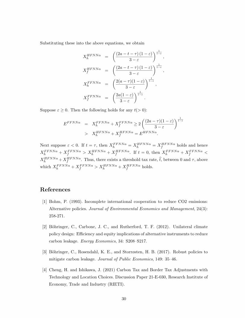
Lemma 1 EHFNNα < EFFNNα holds for t > 0 if ε ≥ 0 and for t > t if ε < 0.

EHFNNα < EFFNNα means that the pollution haven effect leads to positive carbon

leakage between Home and Foreign and increases global emissions.

We obtain the following proposition.

Proposition 5 The following equilibria are possible with a carbon tax: (HN,FN) with

low tax rates and (FN,FN) with high tax rates. Global emissions are greater with

(FN,FN) than with (HN,FN) (i.e., EFFNNα > EHFNNα) if demand is convex ( ε ≥0).

5.2 Carbon tax with a carbon-content tariff (Regime β)

We now introduce the carbon-content tariff in addition to the carbon tax. The carbon-

content tariff increases the effective MCs to export to Home from Foreign, implying a

weaker incentive to choose Foreign as the production location. We can confirm this result

from the following relationship:

(πFFNNα1 − πHFNNα1 )− (πFFNNβ1 − πHFNNβ1 )

= (pNNαh − τ)xNNα1fh − (pNNαh − t)xNNα1hh − ((pNNβh − t− τ)xNNβ1fh − (pNNβh − t)xNNβ1hh ),

which is positive for a given t. Thus, the (lowest) tax rate at which firm 1 is indifferent

between Home and Foreign in Regime β, tβeS1 , is greater than that in Regime α, tαeS1 .

Moreover, EHFNNβ < EHFNNα holds for a given t, because the outputs for the home

market decrease but those for the foreign market do not change. Lemma 1 is valid in

Regime β and hence EHFNNβ < EFFNNβ for t > 0 (i.e., global emissions with (FN,FN)

are greater than those with (HN,FN)) if ε ≥ 0. Thus, if ε ≥ 0, then the carbon-content

tariff is effective at reducing global emissions because it makes firm 1 less likely to locate

itself in Foreign.

In the rest of this subsection, we specifically show that an increase in t can switch

the equilibrium not only from (HN,FN) to (FN,FN) but also from (FN,FN) to

(HA,FN). To this end, we assume linear demand.

27t is a threshold tax rate defined in Appendix.

22

If both firms choose Foreign as their production locations, then the firms are identical.

In Regime α, both firms are independent of t if they produce in Foreign. In Regime β,

however, the profits decrease as t increases. At a certain tax rate, tβ1 , the firms have

an incentive to abate emissions. However, only one of the two firms would adopt the

clean technology at tβ1 . To see this, we simply assume that if only one firm adopts the

clean technology, it is firm 1. Suppose πFFNNβ1 = πFFANβ1 holds at tβ1 . Then we can

verify πFFAAβ2 < πFFANβ2 at tβ1 , implying only one firm (firm 1) would invest in emission

abatement at tβ1 . The other firm (firm 2) would invest in emission abatement at a higher

tax rate, tβ2 .

It should be pointed out that firm 1 has an incentive not only to adopt the clean

technology but also to produce in Home at tβe+1 , where πFFNNβ1 = πHFANβ1 holds. More

importantly, tβe+1 < tβ1 can hold. Since we obtain

πHFANβ1 − πFFANβ1 =4

9

(k2t2 + (τ − ak) t+ τ2

),

πHFANβ1 > πFFANβ1 holds for any t(> 0) if τ ≥ ak.28 Thus, as t rises, the equilibrium

can shift from (HN,FN) to (FN,FN) and then to (HA,FN). Figure 3 (a) illustrates

this case.29

We examine how the equilibrium shift from (FN,FN) to (HA,FN) changes emis-

sions. We obtain

EHFANβ − EFFNNβ = −(1− k)(2a− τ) + k(4k − 3)t

3.

Noting a− 2(t+ τ) > 0, EHFANβ < EFFNNβ holds for a given t. Thus, the relationship

between the tax rate and the emission level is non-monotonic.

It is noteworthy that the equilibrium may switch from (HA,FN) to (FA,FN) as

t further increases. This case is illustrated in Figure 4.30 The equilibrium switch from

(HA,FN) to (FA,FN) increases firm 1’s emissions by 2k2t3 and decreases firm 2’s emis-

sions by kt3 , leading to

EHFANβ − EFFANβ =kt(1− 2k)

3.

28πHFANβ1 > πFFANβ1 holds for any t if (τ − ak)2 − 4k2τ2 < 0.29In Figure 3, we set parameter values as follows: a = 20, τ = 1.5, k = 1/9, and F = 15. Then

we obtain t = 8.5, tβeS1 = 0.122, tβS1 = 1.019, tβe+1 = 2.026, tγe1 = 1.5, tγS1 = 1.782, tγe+1 = 1.807, and

tβ2 = tγ2 = 2.645.30In Figure 4, we set parameter values as follows: a = 20, τ = 1.5, k = 1/6, and F = 7.5. Then we

obtain t = 8.5, tβeS1 = 0.122, tβS1 = 0.536, tβe+1 = 1.086, tβe++1 = 1.251, and tβ2 = 1.289. tβe++

1 is the

threshold tax rate between (HA,FN) and (FA,FN).

23

Figure 3(a): Regime β: (HN,FN) → (FN,FN) → (HA,FN).

Figure 3(b): Regime γ: (HN,FN) → (FN,FN) → (HA,FN).

24

Figure 4: Regime β: (HN,FN) → (FN,FN) → (HA,FN) → (FA,FN).

Thus, EHFANβ < EFFANβ holds for a given t if and only if k > 12 . The change in global

emissions depends on firm 1’s abatement efficiency. If the decrease in firm 2’s output is

replaced by firm 1’s output produced with high abatement efficiency, global emissions

decrease.31

The analysis above establishes the following proposition.

Proposition 6 The following equilibria are possible if a carbon tax is accompanied by a

carbon-content tariff: (HN,FN) with low tax rates, (FN,FN) with medium tax rates,

and (HA,FN) with high tax rates; and EHFNNβ < EFFNNβ > EHFANβ. The carbon-

content tariff weakens firm 1’s incentive to locate itself in Foreign (i.e., tβeS1 > tαeS1 ). A

further increase in t may switch the equilibrium from (HA,FN) to (FA,FN). In this

case, EHFANβ > EFFANβ can hold if k is small.

31This result corresponds to negative carbon leakage in Ma and Yomogida (2019).

25

5.3 Carbon tax coupled with tax refunds at the border and a carbon-

content tariff (Regime γ)

We now introduce carbon-tax refunds in addition to the carbon-content tariff. As

in Regime β, the equilibrium can switch from (HN,FN) to (FN,FN) and then to

(HA,FN) as t increases. Figure 3 (b) illustrates this case.

As firm 1’s effective MCs for its exports become just τ , its incentive to choose Foreign

for production location weakens. That is, tγe1 > tβeS1 > tαeS1 (see Figure 3).32 We can

confirm this result because the following holds for a given t:

(πFFNNβ1 − πHFNNβ1 )− (πFFNNγ1 − πHFNNγ1 )

= (pNNγf − τ)xNNγ1hf − (pNNβf − t− τ)xNNβ1hf > 0.

Although tγe1 > tβe1 , the total emissions with (HN,FN) are larger in Regime γ than in

Regime β for a given t (i.e., EHFNNγ > EHFNNβ for a given t).

When both firms choose Foreign for their production locations, Regime γ and Regime

β are equivalent. Thus, πFFNNγ1 = πFFANγ1 at tβ1 holds. However, regarding the thresh-

old tax rate at which firm 1 has an incentive not only to abate emissions but also to

locate itself in Home, tγe+1 < tβe+1 holds because we have

(πFFNNβ1 − πHFANβ1 )− (πFFNNγ1 − πHFANγ1 )

= (pANγf − τ)xANγ1hf − (pANβf − kt− τ)xANβ1hf > 0

for a given t (compare Figure 3 (a) and (b)).

Note that as in Regime β, the equilibrium may switch from (HA,FN) to (FA,FN)

as t further increases (see Figure 5).33 With linear demand, we can readily verify

EHFNNγ = EFFNNγ(= EFFNNβ),

EHFANγ − EFFNNγ = −(1− k)(2a− τ − 2kt)

3< 0,

EHFANγ = EFFANγ .

We obtain the following proposition.

32We can readily verify tγe1 = τ with linear demand.33In Figure 5, we set parameter values as follows: a = 20, τ = 1.5, k = 3/4, and F = 5. Then we

obtain t = 8.5, tγe1 = 1.5, tγS1 = 2.273, tγe+1 = 2.667, tγe++1 = 3, and tγ2 = 3.280. tγe++

1 is the threshold

tax rate between (HA,FN) and (FA,FN).

26

Figure 5: Regime γ: (HN,FN) → (FN,FN) → (HA,FN) → (FA,FN).

Proposition 7 The following equilibria are possible if a carbon tax is coupled with a

carbon-content tariff and carbon-tax refunds for exports: (HN,FN) with low tax rates,

(FN,FN) with medium tax rates, and (HA,FN) with high tax rates. However, intro-

ducing carbon-tax refunds reduces the range of the tax rate within which firm 1 produces

in Foreign. That is, tαeS1 < tβeS1 < tγe1 and tγe+1 < tβe+1 hold.

6 Conclusion

We have developed a simple two-country, two-firm model to examine how carbon taxes

with BTAs affect outputs, emissions, and the locations of firms in the presence of an

emission-abatement technology (i.e., a clean technology). The two countries (Home and

Foreign) are identical except that only Home introduces carbon pricing. The two firms

are also identical. We specifically examined three policy regimes: i) carbon taxes alone

(no BTAs); ii) carbon taxes accompanied by carbon-content tariffs (partial BTAs); and

iii) carbon taxes coupled with carbon-tax refunds for exports and carbon-content tariffs

(full BTAs).

27

If the firm locations are fixed, the firms’ strategic reaction to a carbon tax is to de-

termine whether or not to abate emissions by adopting the clean technology. According

to our findings, carbon taxes may not be effective in decreasing global emissions. Inter-

estingly, a higher carbon tax rate can result in greater global emissions even with fixed

firm locations. Additionally, high tax rates decrease the incentive to invest in abatement.

Another important message is that cross-border carbon leakage is eliminated in Regime γ

(i.e., full BTAs) but global emissions can be greater than in Regime α (i.e., no BTAs) or

Regime β (i.e., partial BTAs) where cross-border carbon leakage is partially eliminated.

Thus, from the viewpoint of global emission control, carbon leakage is not necessarily

problematic. Moreover, the carbon-tax refund restores the competitiveness of the home

firm in the foreign market but discourages it from making abatement investments.

Under endogenous firm locations, both firms are likely to produce in Foreign in the

presence of a tough carbon tax in Home. Thus, global emissions can increase. BTAs

encourage firms to invest in emission abatement and discourage firms from producing

overseas. This effect is stronger under Regime γ (i.e., full BTAs) than under Regime β

(i.e., partial BTAs). The effect of carbon taxes on global emissions can be non-monotonic

under BTAs. In particular, global emissions could be largest in the middle range of the

tax rate.

Our findings suggest that carbon taxes should be designed with discretion, because

their effects could be different from the conventional wisdom. In particular, carbon taxes

are not very effective in reducing carbon emissions under certain situations. Moreover,

BTAs should be applied cautiously. Even if BTAs eliminate cross-border carbon leak-

age and cost disadvantages for domestic firms, global emissions could increase. Thus,

BTAs may become a disguised form of protection. The practicality of BTAs and their

compatibility with the World Trade Organization (WTO) rules should be deliberated

carefully.

In concluding the paper, two final remarks are in order. First, we have not examined

the optimal policies. This is because the optimal policies depend crucially on how to

evaluate damages from global warming, which in turn depends crucially on a damage

function. For example, if the evaluation of GHG emissions is large enough to dominate

other positive welfare components, then zero emissions are obviously optimal. We can

claim the following with respect to each welfare component.34 The home carbon tax

harms firm 1 unless it adopts the clean technology. The introduction of BTAs for a given

34For details, see Cheng and Ishikawa (2021).

28

tax rate benefits firm 1 if it produces in Home. Global warming is mitigated if and only

if global GHG emissions are reduced. A higher tax does not necessarily result in lower

emissions because the firms may switch their technologies and/or production locations.

Unless firms change technology, less outputs lead to less emissions. However, less outputs

hurt either home or foreign consumers, at the very least. The welfare effects of adopting

the clean technology are less obvious.

Second, to avoid rather straightforward results, we assumed that the two countries

and two firms are symmetric. For example, if firm 2’s emissions per unit of output are

much greater than firm 1’s, carbon leakage from firm 1 to firm 2 should be blocked.

In this case, carbon pricing with assistance for firm 1 is the most likely desirable setup

to cope with climate change. Progress in research on carbon pricing is expected in the

future.

Appendix

To prove Lemma 1, we show that the total output (demand) is greater with (FN,FN)

than with (HN,FN) if ε ≥ 0. From the FOCs of profit maximization, we have

xHFNNα1hh = (pHFNNαh − t)(XHFNNαh )ε, xHFNNα2fh = (pHFNNαh − τ)(XHFNNα

h )ε,

xHFNNα1hf = (pHFNNαf − t− τ)(XHFNNαf )ε, xHFNNα2ff = (pHFNNαf )(XHFNNα

f )ε,

xFFNNα1fh = xFFNNα2fh = (pFFNNαh − τ)(XFFNNαh )ε,

xFFNNα1ff = xFFNNα2ff = (pFFNNαf )(XFFNNαf )ε.

Noting xHFNNα1hi + xHFNNα2fi = XHFNNαi (i = h, f) and xFFNNα1hi + xFFNNα2fi = XFFNNα

i ,

we have

(XHFNNαh )1−ε = 2pHFNNαh − t− τ,

(XHFNNαf )1−ε = 2pHFNNαf − t− τ,

(XFFNNαh )1−ε = 2(pFFNNαh − τ),

(XFFNNαf )1−ε = 2pFFNNαf .

Using (1), we have

pHFNNαh = pHFNNαf =a(1− ε) + t+ τ

3− ε,

pFFNNαh =a(1− ε) + 2τ

3− ε, pFFNNαf =

a(1− ε)3− ε

.

29

Substituting these into the above equations, we obtain

XHFNNαh =

((2a− t− τ) (1− ε)

3− ε

) 11−ε

,

XHFNNαf =

((2a− t− τ) (1− ε)

3− ε

) 11−ε

,

XFFNNαh =

(2(a− τ)(1− ε)

3− ε

) 11−ε

,

XFFNNαf =

(2a(1− ε)

3− ε

) 11−ε

.

Suppose ε ≥ 0. Then the following holds for any t(> 0):

EFFNNα = XFFNNαh +XFFNNα

f ≥ 2

((2a− τ)(1− ε)

3− ε

) 11−ε

> XHFNNαh +XHFNNα

f = EHFNNα.

Next suppose ε < 0. If t = τ , then XFFNNαh = XHFNNα

h = XHFNNαf holds and hence

XFFNNαh + XFFNNα

f > XHFNNαh + XHFNNα

f . If t = 0, then XFFNNαh + XFFNNα

f <

XHFNNαh +XHFNNα

f . Thus, there exists a threshold tax rate, t, between 0 and τ , above

which XFFNNαh +XFFNNα

f > XHFNNαh +XHFNNα

f holds.

References

[1] Bohm, P. (1993). Incomplete international cooperation to reduce CO2 emissions:

Alternative policies. Journal of Environmental Economics and Management, 24(3):

258-271.

[2] Bohringer, C., Carbone, J. C., and Rutherford, T. F. (2012). Unilateral climate

policy design: Efficiency and equity implications of alternative instruments to reduce

carbon leakage. Energy Economics, 34: S208–S217.

[3] Bohringer, C., Rosendahl, K. E., and Storrøsten, H. B. (2017). Robust policies to

mitigate carbon leakage. Journal of Public Economics, 149: 35–46.

[4] Cheng, H. and Ishikawa, J. (2021) Carbon Tax and Border Tax Adjustments with

Technology and Location Choices. Discussion Paper 21-E-030, Research Institute of

Economy, Trade and Industry (RIETI).

30

[5] Conrad, K. (1993). Taxes and subsidies for pollution-intensive industries as trade

policy. Journal of Environmental Economics and Management, 25(2): 121-135.

[6] Copeland, B. R. (1996). Pollution content tariffs, environmental rent shifting, and

the control of cross-border pollution. Journal of International Economics, 40(3-4):

459–476.

[7] Copeland, B. R. and Taylor, M. S. (2005). Free trade and global warming: A

trade theory view of the Kyoto protocol. Journal of Environmental Economics and

Management, 49(2): 205–234.

[8] Cosbey, A., Droege, S., Fischer, C., and Munnings, C. (2019). Developing guidance

for implementing border carbon adjustments: Lessons, cautions, and research needs

from the literature. Review of Environmental Economics and Policy, 13(1): 3–22.

[9] Dijkstra, B. R., Mathew, A. J., and Mukherjee, A. (2011). Environmental regulation:

An incentive for foreign direct investment. Review of International Economics, 19(3):

568–578.

[10] Eichner, T. and Pethig, R. (2015a). Unilateral climate policy with production-

based and consumption-based carbon emission taxes. Environmental and Resource

Economics, 61(2): 141–163.

[11] Eichner, T. and Pethig, R. (2015b). Unilateral consumption-based carbon taxes and

negative leakage. Resource and Energy Economics, 40: 127–142.

[12] Elliott, J., Foster, I., Kortum, S., Munson, T., Perez Cervantes, F., and Weisbach,

D. (2010). Trade and carbon taxes. American Economic Review, 100(2): 465–69.

[13] Erdogan, A. M. (2014). Foreign direct investment and environmental regulations:

A survey. Journal of Economic Surveys, 28(5): 943–955.

[14] Felder, S., and Rutherford, T. F. (1993). Unilateral CO2 reductions and carbon

leakage: The consequences of international trade in oil and basic materials. Journal

of Environmental Economics and Management, 25(2): 162-176.

[15] Fischer, C. and Fox, A. K. (2012). Comparing policies to combat emissions leakage:

Border carbon adjustments versus rebates. Journal of Environmental Economics

and Management, 64(2): 199–216.

31

[16] Forslid, R., Okubo, T., and Ulltveit-Moe, K. H. (2018). Why are firms that export

cleaner? International trade, abatement and environmental emissions. Journal of

Environmental Economics and Management, 91, 166–183.

[17] Furusawa, T., Higashida, K., and Ishikawa, J. (2003). What information is needed

for welfare-enhancing policies under international oligopoly? Japan and the World

Economy, 15, 31–46.

[18] Greaker, M. (2003). Strategic environmental policy; eco-dumping or a green strat-

egy? Journal of Environmental Economics and Management, 45(3):692-707.

[19] Hoel, M. (1997). Environmental policy with endogenous plant locations. Scandina-

vian Journal of Economics, 99(2): 241–259.

[20] Hoel, M. (2005). The triple inefficiency of uncoordinated environmental policies.

Scandinavian Journal of Economics, 107(1): 157–173.

[21] Ishikawa, J. and Kiyono, K. (2006). Greenhouse-gas emission controls in an open

economy. International Economic Review, 47(2): 431–450.

[22] Ishikawa, J., Kiyono, K., and Yomogida, M. (2012). Is emission trading beneficial?

Japanese Economic Review, 63(2), 185-203.

[23] Ishikawa, J., Kiyono, K., and Yomogida, M. (2020). Emissions trading and interna-

tional trade. Discussion Paper 20-E-080, Research Institute of Economy, Trade and

Industry (RIETI).

[24] Ishikawa, J. and Okubo, T. (2010). Environmental and trade policies for oligopolistic

industry in the presence of consumption externalities. International Economy, 14:

59–76.

[25] Ishikawa, J. and Okubo, T. (2011). Environmental product standards in north–south

trade. Review of Development Economics, 15(3): 458–473.

[26] Ishikawa, J. and Okubo, T. (2016). Greenhouse-gas emission controls and interna-

tional carbon leakage through trade liberalization. International Economy, 19:1–22.

[27] Ishikawa, J. and Okubo, T. (2017). Greenhouse-gas emission controls and firm

locations in north–south trade. Environmental and Resource Economics, 67(4):

637–660.

32

[28] Ismer, R. and Neuhoff, K. (2007). Border tax adjustment: a feasible way to support

stringent emission trading. European Journal of Law and Economics, 24(2): 137–

164.

[29] Jaffe, A. B. and Palmer, K. (1997). Environmental regulation and innovation: a

panel data study. Review of Economics and Statistics, 79(4): 610–619.

[30] Jakob, M., Marschinski, R., and Hubler, M. (2013). Between a rock and a hard

place: a trade-theory analysis of leakage under production-and consumption-based

policies. Environmental and Resource Economics, 56(1): 47–72.

[31] Kayalica, M. O. and Lahiri, S. (2005). Strategic environmental policies in the pres-

ence of foreign direct investment. Environmental and Resource Economics, 30(1):

1–21.

[32] Kennedy, P. W. (1994). Equilibrium pollution taxes in open economies with im-

perfect competition. Journal of Environmental Economics and Management 27(1):

49-63.

[33] Kiyono, K., and Ishikawa, J. (2004). Strategic emission tax-quota non-equivalence

under international carbon leakage. In Katayama, S. and Ursprung, H. W. eds.

International Economic Policies in a Globalized World. Springer, Berlin, Heidelberg.

[34] Kiyono, K. and Ishikawa, J. (2013). Environmental management policy under in-

ternational carbon leakage. International Economic Review, 54(3): 1057–1083.

[35] Kortum, S. and Weisbach, D. A. (2017). The design of border adjustments for

carbon prices. National Tax Journal, 70(2): 421.

[36] Kortum, S. and Weisbach, D. A. (2021). Optimal unilateral carbon policy, unpub-

lished manuscript.

[37] Lockwood, B. and Whalley, J. (2010). Carbon-motivated border tax adjustments:

Old wine in green bottles? World Economy, 33(6): 810–819.

[38] Ma, Y. and Yomogida, M. (2019). Border carbon adjustments and foreign direct

investment with technology transfer. unpublished manuscript.

[39] Markusen, J. R. (1975). International externalities and optimal tax structures.

Journal of International Economics, 5(1): 15–29.

33

[40] Markusen, J. R., Morey, E. R., and Olewiler, N. D. (1993). Environmental policy

when market structure and plant locations are endogenous. Journal of Environmen-

tal Economics and Management, 24(1): 69–86.

[41] Markusen, J. R., Morey, E. R., and Olewiler, N. D. (1995). Competition in regional

environmental policies when plant locations are endogenous. Journal of Public Eco-

nomics, 56(1): 55–77.

[42] Mrazova, M. and Neary, P. (2017). Not so demanding: Demand structure and firm

behavior. American Economic Review, 107(12): 3835–3874.

[43] Perino, G. and Requate, T., (2012). Does more stringent environmental regulation

induce or reduce technology adoption? When the rate of technology adoption is

inverted U-shaped. Journal of Environmental Economics and Management, 64(3),

456-467.

[44] Tsakiris, N., Hatzipanayotou, P., and Michael, M. S. (2019). Border tax adjustments

and tariff-tax reforms with consumption pollution. Journal of Public Economic

Theory, 21(6): 1107–1125.

[45] Ulph, A. and Ulph, D. (2007). Climate change–environmental and technology poli-

cies in a strategic context. Environmental and Resource Economics, 37(1):159-180.

[46] Yomogida, M. and Tarui, N. (2013). Emission taxes and border tax adjustments for

oligopolistic industries. Pacific Economic Review, 18(5): 644–673.

[47] Zeng, D. Z. and Zhao, L. (2009). Pollution havens and industrial agglomeration.

Journal of Environmental Economics and Management, 58(2): 141–153.

34