Cardiac C-Arm Computed Tomography:Motion Estimation and ... · Teri Moore and Amin Al-Ahmad. Erin...

Cardiac C-Arm Computed Tomography:Motion Estimation

andDynamic Reconstruction

Der Technischen Fakultät derUniversität Erlangen–Nürnberg

zur Erlangung des Grades

DOKTOR–INGENIEUR

vorgelegt von

Marcus Prümmer

Erlangen 2009

Deutscher Titel:C-Arm-Computertomographiein der Herzbildgebung:

Bewegungsschätzungund

dynamische Rekonstruktion

Als Dissertation genehmigt von derTechnischen Fakultät der

Universität Erlangen-Nürnberg

Tag der Einreichung: 04.05.2009Tag der Promotion: 02.09.2009Dekan: Prof. Dr.-Ing. habil. J. HuberBerichterstatter: Prof. Dr.-Ing. J. Hornegger

Assoc. Prof. R. Fahrig (Ph. D.)

Abstract

Generatingthree dimensional images of the heart during interventional procedures is a sig-nificant challenge. In addition to real-time fluoroscopy, angiographic C-arm systems canalso be used to generate 3-D/4-D CT images on the same system. One protocol for car-diac Computed Tomography (CT) uses electrocardiogram (ECG) triggered multi-sweepscans. A 3-D volume of the heart at a particular cardiac phase is reconstructed by theFeldkamp, Davis and Kress (FDK) algorithm using projection images with retrospectiveECG gating. In this thesis we introduce a unified framework for heart motion estimationand dynamic cone-beam reconstruction using motion corrections. Furthermore, theoreticalconsiderations about dynamic filtered backprojection (FBP) as well as dynamic algebraicreconstruction techniques (ART) are presented, discussed and evaluated. Dynamic CTreconstruction allows to improve temporal resolution and image quality using image pro-cessing. It is limited by C-arm device hardware like rotation speed.

The benefits of motion correction are: (1) increased temporal and spatial resolutionby removing cardiac motion which may still exists in the ECG-gated data sets, and (2)increased signal-to-noise ratio (SNR) by using more projection data than is used in stan-dard ECG gated methods. Three signal enhancing reconstruction methods are introducedthat make use of all of the acquired projection data to generate a time resolved 3-D re-construction. The first averages all motion corrected backprojections; the second and thirdperform a weighted averaging according to: (1) intensity variations and (2) temporal dis-tance to a time resolved and motion corrected reference FDK reconstruction. In a studyseven methods are compared: non-gated FDK, ECG-gated FDK, ECG-gated and motioncorrected FDK, the three signal enhancing approaches, and temporally aligned and av-eraged ECG-gated FDK reconstructions. The quality measures used for comparison arespatial resolution and SNR.

Additionally new dynamic algebraic reconstruction techniques (ART) are introduced,compared to dynamic Filtered Backprojection (FBP) methods and evaluated. In ART wemodel the objects motion either using a dynamic projector model or a dynamic grid of theobject, defining the spatial sampling of the reconstructed density values. Both methodsare compared to each other as well as to dynamic FBP. Spatial and temporal interpolationissues in dynamic ART and FBP and the computational complexity of the algorithms areaddressed. The subject-specific motion estimation is performed using standard non-rigid3-D/3-D and novel 3-D/2-D registration methods that have been specifically developed forthe cardiac C-arm CT reconstruction environment. In addition theoretical considerationsabout fast shift-invariant filtered backprojection methods in dependency of an affine, ray-affine and non-rigid motion model are presented.

Evaluation is performed using phantom data and several animal models. We show thatdata driven and subject-specific motion estimation combined with motion correction candecrease motion-related blurring substantially. Furthermore, SNR can be increased by upto 70% while maintaining spatial resolution at the same level as it is provided by the ECG-gated FDK. The presented framework provides excellent image quality for cardiac C-armCT. The thesis contributes to an improved image quality in cardiac C-arm CT and providesseveral methods for dynamic FBP and ART reconstruction.

ÜbersichtDie Rekonstruktion von dreidimensionalen Bildern des Herzens während eines interven-tionellen Eingriffes ist eine große Herausforderung. Auf demselben C-Arm Angiogra-phiesystem können zusätzlich zur Echtzeitfluroskopie jetzt auch 3-D/4-D Bilder generiertwerden. Ein Protokoll für C-Arm Computertomographie in der Herzbildgebung verwen-det elektrokardiogram (EKG) getriggerte Mehrfachumläufe. Ein 3-D Bild des Herzenseiner speziellen Herzphase wird mittels der Feldkamp (FDK) Methode aus einer retro-spektiv getriggerten Projektionsmenge rekonstruiert. Diese Arbeit führt eine kombinierteSchätzung der Herzbewegung und dynamische Kegelstrahlrekonstruktion unter Verwen-dung von Bewegungskorrektur ein. Desweiteren werden theoretische Betrachtungen überDynamische Gefilterte Rückprojektion sowie Dynamische Algebraische Rekonstruktionpräsentiert, diskutiert und ausgewertet. Die Dynamische Rekonstruktion erlaubt hardwarebedingte Einschränkungen wie Rotationsgeschwindigkeit und die daraus resultierende zeit-liche Auflösung sowie Bildqualität mittels Bildverarbeitung zu verbessern.

Die Vorteile der Bewegungskorrektur sind: (1) erhöhte zeitliche und räumliche Au-flösung durch Entfernen der verbleibenden Herzbewegung eines EKG-getriggerten Pro-jetionsdatensatzes und (2) verbessertes Signal zu Rauschverhältnis (S/R) durch Verwen-dung zusätzlicher Projektionsdaten. Drei Methoden zur Verbesserung des S/R werdenvorgestellt. Diese beziehen alle aufgenommenen Projektionsbilder in eine zeitaufgelösteRekonstruktion ein. Die erste Methode mittelt alle bewegungskorrigierten Projektionen,die Zweite und Dritte führen eine Mittelung entsprechend (1) der Intensitätsvariation und(2) dem zeitlichem Abstand zu einer zeitlich aufgelösten und bewegungskorrigierten Ref-erenzrekonstruktion. In einer Studie werden sieben FDK-Methoden verglichen: nicht-getriggert, EKG-getriggert, EKG-getriggert und bewegungskorrigiert, drei S/R verbess-ernde Methoden und EKG-getriggerte zeitlich ausgerichtete und gemittelte Rekonstruktio-nen. Es werden Ortsauflösung und S/R verglichen.

Zusätzlich werden neue Dynamische Algebraische Rekonstruktionstechniken (ART)eingeführt, evaluiert und mit der Dynamischen Gefilterten Rückprojektion verglichen. InART kann die Objektbewegung entweder mittels eines dynamischen Projektors oder einesdynamischen Objektgitters modelliert werden. Beide Methoden werden zueinander undzur Dynamischen Gefilterten Rückprojektion verglichen. Räumliche und zeitliche Inter-polationsfaktoren sowie die Komplexität der Algorithmen werden erläutert. Patienten-speziefische Bewegungsschätzung wird mittels herkömmlicher nicht-starrer 3D/3D undneuentwickelter 3D/2D Registrierung durchgeführt. Diese wurden speziell für C-Arm CTAnwendungen entwickelt. Theoretische Zusammenhänge zur Herleitung schneller undverschiebungsunabhängiger Filter für die Gefilterte Rückprojektion in Abhängigkeit vonaffinen, strahl-affinen und nicht-starren Bewegungsmodellen werden aufgezeigt.

Die Auswertung wurde mit Phantomdaten sowie verschiedener Tiermodelle durchge-führt. Es wird gezeigt, dass mittels patientenspeziefischer Bewegungsschätzung kom-biniert mit Bewegungskorrektur die durch Bewegung verursachten Artefakte erheblich re-duziert werden können. Das S/R kann bis zu 70% erhöht werden, während die Ortsauflö-sung mit den von herkömmlichen EKG-getriggerten Rekonstruktionsverfahren verglichenwerden kann. Das in dieser Arbeit vorgestellte Framework bietet verbesserte Bildqualitätfür Herzbildgebung unter Verwendung von C-Arm CT. Ein wesentlicher Beitrag der Arbeitliegt in der Verbesserung der Bildqualität sowie der Einführung verschiedenster Algorith-men für die Dynamische Gefilterte Rückprojektion und Dynamische ART.

Acknowledgments

This thesis started in October 2003, a time when cardiac C-arm CT was probably alreadyin the mind of some innovative engineers and rather far away from an applicable productused in the interventional suite. At the time finishing this thesis I am enthusiastic aboutthe fact that meanwhile many new applications for cardiac C-arm CT arise and this newtechnology is established in the interventional room. First attempts in cardiac reconstruc-tion using a C-arm considered the data from a single rotation scan. The arising imageprocessing problems were oriented in the field of symbolic reconstruction or a sparse pro-jection reconstruction. In cooperation with Siemens AG, Medical Solutions in Forchheim(since 2005) the topic of this thesis has been focused on the improvement in image qualityfor multi-segment cardiac C-arm CT. Since then many things changed, even their name toSiemens AG, Healthcare Sector.I deeply appreciate the support by Prof. Dr.-Ing. Joachim Hornegger, who became an im-portant mentor in my life. I have learned many important things from him in the fieldof research and business and how to combine both. As an exemplary networker and for-mer Siemens Medical Solutions employee, he established the joint cooperation betweenthe Department of Radiology, Stanford University and Siemens AG, Healthcare Sector,Forchheim. It turned out that this cooperation provided the basis for many of the problemformulations as addressed in this work and provided a huge amount of in vivo and firsthuman data, that was very valuable for my thesis.At this point I greatfully thank my co-supervisor Rebecca Fahrig, Associate Professor ofRadiology at Stanford University, for supporting me in many ways like valuable discus-sions about cardiac C-arm CT, data acquisition in her C-arm lab and many other things. Forassistance in the Stanford C-arm lab I greatfully thank Erin Girard-Hughes, Lars Wigström,Teri Moore and Amin Al-Ahmad. Erin for building the quite helpful plastic phantom, ac-quiring tons of data and in general for the pleasant cooperation. Furthermore I thank TeriMoore, Wendy Baumgardner and Diane Howard for technical assistance at Stanford Uni-versity. This research at Stanford University was also supported by NIH R01 EB003524,Siemens AG, Healthcare Sector, and the Lucas Foundation. The author thanks Dr. NorbertStrobel for supporting first investigations of C-arm calibration issues of a separated for-ward and backward sweep calibration. Furthermore, I would like to thank him for a greattime of doing research together in the Stanford Axiom Lab. Many ideas included in thiswork are a result of several tasteful and fruitful working lunch.I am also deeply grateful to Dr. Günter Lauritsch and Dr. Jan Boese, both working atSiemens AG, Healthcare Sector, for co-financing my work and giving me the chance tocontribute to recent developments in cardiac C-arm CT. I appreciate many valuable paperreviews and comments by Günter and also for guiding me in terms of focusing on specificand very interesting topics for this thesis. I can’t tell how much input from him is reflectedin this thesis, but I am sure it’s a whole bunch of ideas. There are many other people atSiemens I would like to thank. For example Dr. Benno Heigl, Dr. Marcus Pfister, Dr. Hol-ger Kunze and Dr. Frank Dennerlein for providing data or inspiring discussions.The reason for having a good time at the Chair of Pattern Recognition (LME) during thelast years is probably the pleasant company of my colleagues and friends at the LME. Ithank Eva Kollorz and Florian Jäger for proof-reading this thesis and many valuable com-ments.

The support from my roommates Volker Daum and Dieter Hahn is alsounpayable. Theyprovided many helpful comments during the development of algorithms and proof-readingof this thesis and gave programming support in times when time was short and the compilerrejected my source-code.For the development of a multigrid technique to accelerate cone-beam ART I thank Dr. Har-ald Köstler for the good cooperation. In addition we thank the Bavaria California Technol-ogy Center (BaCaTec) for financial support and HipGraphics, Towson, Maryland, USA forthe volume rendering software InSpace.Finally, I thank my parents and especially my girlfriend for the patience and mental supportduring the last years.

Criesbach, 2nd May 2009 Marcus Prümmer

Contents

1 Intr oduction 11.1 Interventional Cardiology . . . . . . . . . . . . . . . . . . . . . . . . . 1

1.1.1 Clinical Workflow . . . . . . . . . . . . . . . . . . . . . . . . . 21.1.2 Cardiac C-arm CT and Related Image Processing . . . . . . . . . 2

1.2 C-arm CT: A Short History . . . . . . . . . . . . . . . . . . . . . . . . 31.3 Related Work . . . . . . . . . . . . . . . . . . . . . . . . . . . . . . . . 5

1.3.1 Motion Model Estimation . . . . . . . . . . . . . . . . . . . . . 61.3.2 Dynamic CT Reconstruction . . . . . . . . . . . . . . . . . . . . 91.3.3 SNR Enhanced Reconstruction . . . . . . . . . . . . . . . . . . . 111.3.4 Discussion . . . . . . . . . . . . . . . . . . . . . . . . . . . . . 11

1.4 Contributions to Cardiac C-arm CT . . . . . . . . . . . . . . . . . . . . 121.5 Heart Anatomy and Cardiac Cycle . . . . . . . . . . . . . . . . . . . . . 13

1.5.1 Anatomy . . . . . . . . . . . . . . . . . . . . . . . . . . . . . . 131.5.2 Cardiac Cycle . . . . . . . . . . . . . . . . . . . . . . . . . . . . 14

1.6 Document Overview . . . . . . . . . . . . . . . . . . . . . . . . . . . . 15

2 Multi-segment Cardiac C-arm CT 212.1 Acquisition Protocol . . . . . . . . . . . . . . . . . . . . . . . . . . . . 22

2.1.1 Series of Alternating Forward and Backward Runs . . . . . . . . 222.1.2 Scan Parameters . . . . . . . . . . . . . . . . . . . . . . . . . . 232.1.3 Practical Aspects . . . . . . . . . . . . . . . . . . . . . . . . . . 23

2.2 Cardiac Phase Identification . . . . . . . . . . . . . . . . . . . . . . . . 272.2.1 Electrocardiogram . . . . . . . . . . . . . . . . . . . . . . . . . 272.2.2 Heart Rate Dependency of the Cardiac Phase . . . . . . . . . . . 282.2.3 Image-Based Gating . . . . . . . . . . . . . . . . . . . . . . . . 29

2.3 Retrospective ECG-Gating . . . . . . . . . . . . . . . . . . . . . . . . . 30

3 Heart Motion Estimation 353.1 Non-Rigid 3-D/3-D Registration . . . . . . . . . . . . . . . . . . . . . . 37

3.1.1 Motivation . . . . . . . . . . . . . . . . . . . . . . . . . . . . . 373.1.2 Cardiac Phase Selection . . . . . . . . . . . . . . . . . . . . . . 383.1.3 Pre-Processing . . . . . . . . . . . . . . . . . . . . . . . . . . . 383.1.4 Non-rigid Registration . . . . . . . . . . . . . . . . . . . . . . . 393.1.5 Deformation Field Interpolation . . . . . . . . . . . . . . . . . . 423.1.6 Temporal Regularization . . . . . . . . . . . . . . . . . . . . . . 443.1.7 Deformation Regridding via Adaptive Sampling . . . . . . . . . 47

i

3.2 Non-rigid 3-D/2-D Registration . . . . . . . . . . . . . . . . . . . . . . 513.2.1 Distance Measure Objectives . . . . . . . . . . . . . . . . . . . . 523.2.2 Mono-modal Distance Measure . . . . . . . . . . . . . . . . . . 523.2.3 Multi-modal Distance Measure . . . . . . . . . . . . . . . . . . . 543.2.4 Heuristic Schemes . . . . . . . . . . . . . . . . . . . . . . . . . 58

4 Dynamic Computed Tomography 614.1 Introduction . . . . . . . . . . . . . . . . . . . . . . . . . . . . . . . . . 61

4.1.1 Problem Statement . . . . . . . . . . . . . . . . . . . . . . . . . 614.1.2 Scan Geometry . . . . . . . . . . . . . . . . . . . . . . . . . . . 64

4.2 Fourier Slice Theorem . . . . . . . . . . . . . . . . . . . . . . . . . . . 664.2.1 Static Geometry . . . . . . . . . . . . . . . . . . . . . . . . . . 664.2.2 Dynamic Geometry . . . . . . . . . . . . . . . . . . . . . . . . . 68

4.3 Filtered Backprojection . . . . . . . . . . . . . . . . . . . . . . . . . . . 714.3.1 Static Geometry . . . . . . . . . . . . . . . . . . . . . . . . . . 714.3.2 Dynamic Geometry . . . . . . . . . . . . . . . . . . . . . . . . . 73

4.4 Feldkamp-Extension for Dynamic Reconstruction . . . . . . . . . . . . . 764.4.1 Feldkamp . . . . . . . . . . . . . . . . . . . . . . . . . . . . . . 764.4.2 Dynamic Filtered Backprojection (MC-FDK) . . . . . . . . . . . 77

4.5 Algebraic Reconstruction . . . . . . . . . . . . . . . . . . . . . . . . . . 794.5.1 System Matrix . . . . . . . . . . . . . . . . . . . . . . . . . . . 794.5.2 Iteration using Cimmino’s Method . . . . . . . . . . . . . . . . . 924.5.3 Iteration using Dynamic Geometry . . . . . . . . . . . . . . . . . 934.5.4 Iteration using Dynamic Object Grid . . . . . . . . . . . . . . . . 94

5 SNR Enhanced Reconstruction 955.1 Averaging Scheme (SNR0) . . . . . . . . . . . . . . . . . . . . . . . . . 965.2 Cardiac Phase Variance Scheme (SNR1) . . . . . . . . . . . . . . . . . 965.3 Intensity Scheme (SNR2) . . . . . . . . . . . . . . . . . . . . . . . . . 975.4 Algorithmic Summary of SNR Enhanced Reconstruction . . . . . . . . . 975.5 Algorithmic Variations . . . . . . . . . . . . . . . . . . . . . . . . . . . 975.6 Computational Complexity . . . . . . . . . . . . . . . . . . . . . . . . . 98

6 Evaluation of Motion Estimation 1036.1 Methods and Materials . . . . . . . . . . . . . . . . . . . . . . . . . . . 103

6.1.1 Plastic Phantom . . . . . . . . . . . . . . . . . . . . . . . . . . . 1036.1.2 Porcine Models . . . . . . . . . . . . . . . . . . . . . . . . . . . 105

6.2 ECG-gating . . . . . . . . . . . . . . . . . . . . . . . . . . . . . . . . . 1066.2.1 Temporal Resolution: In Vivo Study . . . . . . . . . . . . . . . . 1066.2.2 Comparison between Relative RR-Peak and Absolute Time . . . 1066.2.3 Image-Based Gating . . . . . . . . . . . . . . . . . . . . . . . . 108

6.3 Non-rigid 3-D/3-D Registration . . . . . . . . . . . . . . . . . . . . . . 1096.3.1 Initial ECG-gated Reconstructions . . . . . . . . . . . . . . . . 1096.3.2 Temporal Interpolation of MVF . . . . . . . . . . . . . . . . . . 1116.3.3 Temporal Regularization . . . . . . . . . . . . . . . . . . . . . . 1136.3.4 Deformation Regridding by Adaptive Supersampling . . . . . . . 1156.3.5 Investigation of X-ray Dose Sensitivity . . . . . . . . . . . . . . 117

ii

6.3.6 An Ultrasound Evaluation Framework For Motion EstimationAc-curacy . . . . . . . . . . . . . . . . . . . . . . . . . . . . . . . 118

6.4 Non-rigid 3-D/2-D Registration . . . . . . . . . . . . . . . . . . . . . . 1296.4.1 Methods and Materials . . . . . . . . . . . . . . . . . . . . . . . 1296.4.2 Multi-modal Distance Measure . . . . . . . . . . . . . . . . . . . 1316.4.3 Heuristic Method: Mono-modal Approximation . . . . . . . . . . 1376.4.4 Heuristic Method: Multi-modal Approximation . . . . . . . . . . 1386.4.5 Discussion . . . . . . . . . . . . . . . . . . . . . . . . . . . . . 140

7 Evaluation of Dynamic FBP Algorithms 1457.1 Methods and Materials . . . . . . . . . . . . . . . . . . . . . . . . . . . 145

7.1.1 Virtual Shepp-Logan Phantom . . . . . . . . . . . . . . . . . . . 1457.1.2 Porcine Models . . . . . . . . . . . . . . . . . . . . . . . . . . . 1457.1.3 Evaluation of Image Quality . . . . . . . . . . . . . . . . . . . . 147

7.2 Evaluation Studies . . . . . . . . . . . . . . . . . . . . . . . . . . . . . 1477.2.1 Warping in Projection- vs. Backprojection Space . . . . . . . . . 1477.2.2 MC-FDK Algorithm: Simulation Study using the FORBILD Phan-

tom . . . . . . . . . . . . . . . . . . . . . . . . . . . . . . . . . 1487.2.3 Plastic Phantom: Comparison of Dynamic FBP Methods . . . . . 1497.2.4 Animal Study: Comparison of Dynamic FBP Methods . . . . . . 1527.2.5 Animal Study: Single-Sweep Correction Assuming Known MVF 1567.2.6 Animal Study: Comparison of EG-FDK6 × 4s and4 × 4s MC-

FDK Reconstruction . . . . . . . . . . . . . . . . . . . . . . . . 1587.2.7 Animal Study: MC-FDK Reconstruction using4×5sProtocol and

Full Temporal Resolution . . . . . . . . . . . . . . . . . . . . . 1607.2.8 Animal Study: SNR0 Reconstruction Method . . . . . . . . . . . 161

7.3 Discussion and Conclusions . . . . . . . . . . . . . . . . . . . . . . . . 1637.3.1 Discussion . . . . . . . . . . . . . . . . . . . . . . . . . . . . . 1637.3.2 Conclusions . . . . . . . . . . . . . . . . . . . . . . . . . . . . . 164

8 Evaluation of Dynamic ART 1678.1 Evaluation Methods . . . . . . . . . . . . . . . . . . . . . . . . . . . . . 1678.2 System Matrix Properties . . . . . . . . . . . . . . . . . . . . . . . . . . 168

8.2.1 Structure ofATA . . . . . . . . . . . . . . . . . . . . . . . . . . 1688.2.2 Point-Spread-Function . . . . . . . . . . . . . . . . . . . . . . . 1698.2.3 Singular Values . . . . . . . . . . . . . . . . . . . . . . . . . . . 1698.2.4 Sampling Structure . . . . . . . . . . . . . . . . . . . . . . . . . 170

8.3 Simulation Study . . . . . . . . . . . . . . . . . . . . . . . . . . . . . . 1708.4 Discussion and Conclusions . . . . . . . . . . . . . . . . . . . . . . . . 170

9 Summary and Outlook 1779.1 Summary . . . . . . . . . . . . . . . . . . . . . . . . . . . . . . . . . . 177

9.1.1 Theory . . . . . . . . . . . . . . . . . . . . . . . . . . . . . . . 1779.1.2 Evaluation . . . . . . . . . . . . . . . . . . . . . . . . . . . . . 180

9.2 Outlook . . . . . . . . . . . . . . . . . . . . . . . . . . . . . . . . . . . 182

iii

A Appendix 185A.1 A Full Multigrid Technique to Accelerate ART . . . . . . . . . . . . . . 185

A.1.1 Problem Description . . . . . . . . . . . . . . . . . . . . . . . . 185A.1.2 The Multigrid Algorithm . . . . . . . . . . . . . . . . . . . . . . 186A.1.3 Experimental Results . . . . . . . . . . . . . . . . . . . . . . . . 188A.1.4 Conclusion . . . . . . . . . . . . . . . . . . . . . . . . . . . . . 189

List of Figures 191

List of Tables 195

Notation and Abbreviations 197

Bibliography 201

Index 209

iv

Chapter 1

Intr oduction

We start with some general notes about interventional cardiology and present some clini-cal applications. A typical interventional workflow in cardiology is described, before theapplication of cardiac C-arm CT in cardiology is motivated. Furthermore, a brief historyin C-arm development is listed and related work to this thesis is discussed. A brief sum-mary of the major contributions to cardiac C-arm CT, as introduced in this thesis, is given.A quick anatomical review of the heart as relevant for the technical aspects in this workprovides the medical background knowledge. The introduction ends with a short chapteroverview.

1.1 Interventional Cardiology

Many procedures on the heart are performed using a catheter where access to the heartis gained minimally invasively via a large artery or vein. These procedures make use ofvisualization using X-ray fluoroscopy in combination with recently developed 3-D imag-ing techniques. For example, minimally invasive cardiac procedures include stenting forthe treatment of atherosclerosis, valvuloplasty for the dilation of narrowed cardiac valves,angioplasty of great vessels, and treatments of atrial fibrillation (AF) and ventricular fib-rillation. C-arm computed tomography (C-arm CT) is presented as the next generation ofimaging technology available in the angiography suite. It provides a platform for manyof the three-dimensional mapping and navigational tools that supports the physician dur-ing the above mentioned procedures. For example, the volumetric visualization of thecoronary sinus and coronary arteries provides valuable information for many pacing pro-cedures. Cardiac resynchronization therapy (CRT) using left- (LV) or biventricular pacingis widely applied in selected heart failure patients, however, transvenous LV-lead place-ment into coronary sinus (CS) branches can be challenging, as reported by [Gutleben08].Recently developed single rotation C-arm acquisition protocols with adapted motion com-pensation techniques provide improved image quality of the coronary sinus as introducedby [Rohkohl08MIC].Recently, new imaging protocols have investigated the visualization of human heart struc-tures, including the left atrium, left atrial appendage and pulmonary veins, left ventricle,and coronary vessels, that are important for guidance of atrial fibrillation (AF) ablation orbiventricular pacing procedures. For these procedures a 3-D visualization of contrastedventricles becomes very important. Catheter ablation is becoming an established standard-

1

2 Chapter 1. Introduction

of-care treatment for many cardiac arrhythmias, but remains a complicated procedure thatcould benefit from 3-D cardiac C-arm CT images tremendously. For example, the re-cently introduced multi-segment C-arm CT acquisition protocol [Lauritsch06TMI] pro-vides ECG-gated volumetric reconstructions to visualize the left atrium and pulmonaryveins for the benefit of pulmonary vein isolation procedures.

1.1.1 Clinical Workflow

A catheter is inserted and guided towards the heart while the doctor is watching the positionof the catheter on the fluoroscopic system. The catheter position is changed multiple timesduring the procedure. For visual feedback of the catheter position and the vessel tree dye isinjected via the catheter during the navigation. Once the right position is reached, the doc-tor can proceed with the treatment and then remove carefully the catheter. The benefits ofsuch minimally invasive procedures include faster recovery and decreased infection ratesto the patient and quicker out-patient procedures for the hospital. Physicians are trained in-tensively since an excellent knowledge about the vessel system and anatomical structure isdesirable for a fast and reliable catheter navigation. To reduce radiation dose, visualizationusing fluoroscopy is only performed at positions of complex vessel structures, whereas,often the navigation is done blind and based on experience.

1.1.2 Cardiac C-arm CT and Related Image Processing

A major motivation for bringing cardiac C-arm CT into the interventional suite is the elim-ination of the need for a preoperative CT scan. Thus radiation dose can be reduced and animmediate 3-D image of the heart’s anatomy is provided. In some cases there is the need toperform necessary follow up scans during the procedure. The acquisition protocols in in-terventional cardiology are specifically adapted to the concrete treatment that is performed.Degrees of freedom are, for example, contrast injection site, total contrast injected, injec-tion rate, C-arm rotation speed (slow vs. fast), single rotation or multi-segment acquisition,and reconstruction parameters.Access to intra-procedural 3-D images in the interventional suite is becoming more im-portant as minimally invasive cardiac procedures increase in complexity. RetrospectivelyECG-gated cardiac C-arm CT has recently been developed [Lauritsch06TMI], allowing asingle C-arm imaging system to provide both real-time (30 frames/s) fluoroscopy and 3-Dvolume CT images of the heart during a procedure. The imaging protocol for this 3-Dvolume imaging approach is to acquire 2-D projection images during sweeps around theobject while simultaneously recording the ECG signal. A 3-D volume reconstruction of aparticular cardiac phase is accomplished by choosing the projection at each angle of theset of projections that is closest to the phase of interest, and then using the standard Feld-kamp reconstruction algorithm (FDK) [Feldkamp84] to generate the 3-D volume. Current3-D image quality, as defined by signal-to-noise ratio (SNR) and motion-related bluring(MRB), is determined by the total imaging time (which must be within a single breathhold), the time per sweep, the detector readout rate, and the dose per projection. Theseparameters determine the number of projections (and therefore the dose) and the temporalspread of the projection data that contribute to a single reconstructed volume at a givencardiac phase. Improvement of image quality for these typically view-starved 3-D recon-

1.2. C-arm CT: A Short History 3

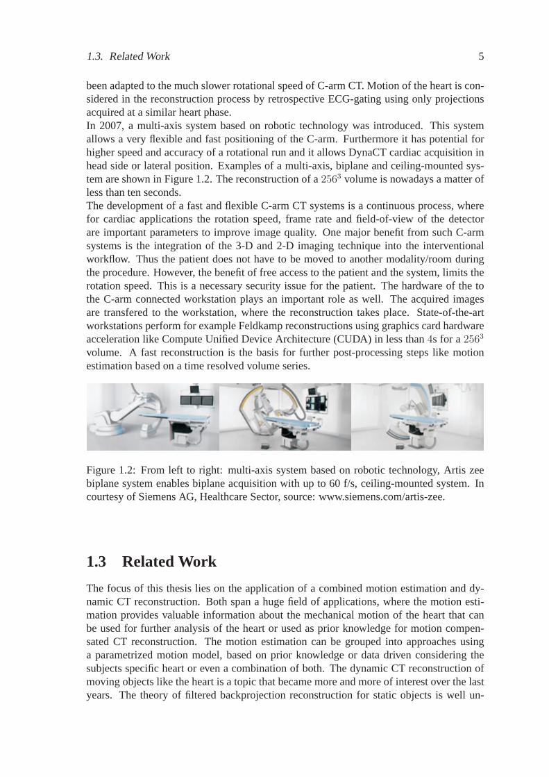
structions (e.g.∼ 200 views per volume as compared to∼ 1000 for clinical CT) may beparticularly important if there is a need to use automatic segmentation and/or 2-D/3-D im-age registration algorithms during the intervention.One approach to improve image quality and to increase dose efficiency of the ECG-gatedC-arm CT imaging protocol is to use all of the projection data acquired to produce a singlevolume at the cardiac phase of interest. Such an approach increases the SNR of the recon-structed volume, but requires knowledge of and correcton for the motion of the object inorder to limit MRB. Many methods for motion estimation and for motion correction forboth respiratory and cardiac motion in 3-D reconstructed images have been developed. Asummary of the current state of the art is presented in the following sections. In general,the motion is first modeled via a mathematical model, using dense deformation fields orusing spline models. In the second step, a reconstruction method that considers the motionis applied to improve the quality of the reconstruction. This combination of motion estima-tion and dynamic reconstruction reduces MRB and can improve image quality in cardiacC-arm CT. An illustration of motion estimation and dynamic CT reconstruction is shownin Figure 1.1.

1.2 C-arm CT: A Short History

A brief overview is given about the development in C-arm CT from the first steps in 3-DC-arm reconstruction to the recently introduced cardiac C-arm CT applications. Pushingthe limitations of the C-arm hardware raises new software applications like SNR enhanced-and motion compensated cardiac reconstruction.

C-arm CT first emerged as a useful high-contrast imaging modality in the late 1990s.In 2000 [Wiesent00] described the possibilities of fast 3-D-reconstruction of high-contrastobjects with high spatial resolution from only a small series of two-dimensional (2-D) pla-nar radiographs using a C-arm system. The reconstruction of a2563 volume took severalminutes. First examples for cranial vessel imaging from some clinical tests were presented.The main issues pointed out in their work was the calibration of the mechanically unstableC-arm system and a trade-off between image quality and computation time. The spatialresolution for high contrast objects like bones or vessels filled with contrast agent had beenshown to be 0.1 mm - 0.3 mm. Their work was targeting applications in medical diagnosis,therapy planning, and interventional procedures.

3-D cardiac imaging is still performed using fast rotating cardiac CT scanners. Anadaptation of the Feldkamp [Feldkamp84] method to cone-beam projections acquired witha C-arm system was introduced by [Grass99]. Their work presented reconstruction resultsobtained along real source-detector trajectories of a C-arm system and compared the re-sults to reconstructions obtained from projections acquired from a full-circular trajectoryand from one consisting of two full orthogonal circles, which fulfilled Tuy’s [Tuy83] suf-ficiency condition. The first biplane C-arm (Siemens AXIOM Artis dBA) for universalprocedures in angiography for neuroradiologists, neurosurgeons, neurologists and cardi-ologists was introduced in 2004. An enhancement for C-arm angiography systems thatallows soft tissue imaging in the angio-suite was introduced in 2004 too, named DynaCT(Siemens AXIOM Artis FD systems). It allows clinicians to perform angiographic com-


Intervention

sweep 1 (fw)sweep 2 (bw)sweep 3 (fw)sweep 4 (bw)

C-arm rotation

EC

G

continuous timeline trigger delay

start t=0

t=4st=5s

t=9st=10s

t=14st=15s

t=19s

ECG-gated Short-ScanSets of Projections ...

3-D + t Reconstruction

t=0.8 t=0.3

...

Creation of 4-D Motion Model: Motion Estimation using Non-rigid Registration

Com

ple

teA

cquired P

roje

ction D

ata

4-D Motion Model

SNR-enhanced andMotion Corrected Reconstruction

Improved Segmentation of Ventricles

Reduced Motion Related Blurring

Improved SNR

Dynamic CT Reconstruction

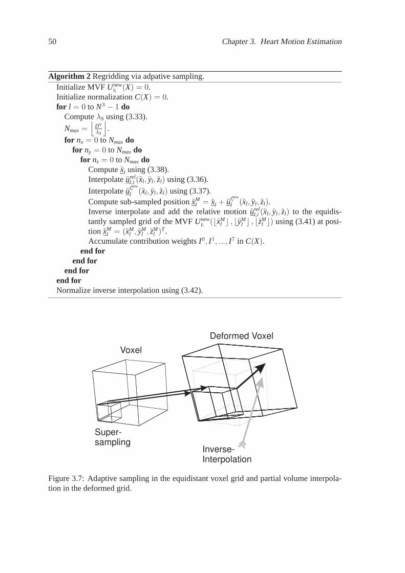
Figure1.1: Illustration of dynamic CT reconstruction in application to cardiac C-arm CT.The example shows four subsequent forward (fw) and backward (bw) sweeps, each singlesweep takes four seconds (short4× 4s).

puted tomography directly in the angio-suite. Image acquisition could be achieved witha 10 second C-arm spin. The system enabled visualization of tissue differentiation in therange of 10 Hounsfield Units (HU).In 2006, a new approach for cardiac imaging was introduced by [Lauritsch06TMI]. It takesadvantage of an improved contrast resolution and is based on intravenous contrast injec-tion. The method is an analogue to multi-segment reconstruction in cardiac CT that had

1.3. Related Work 5

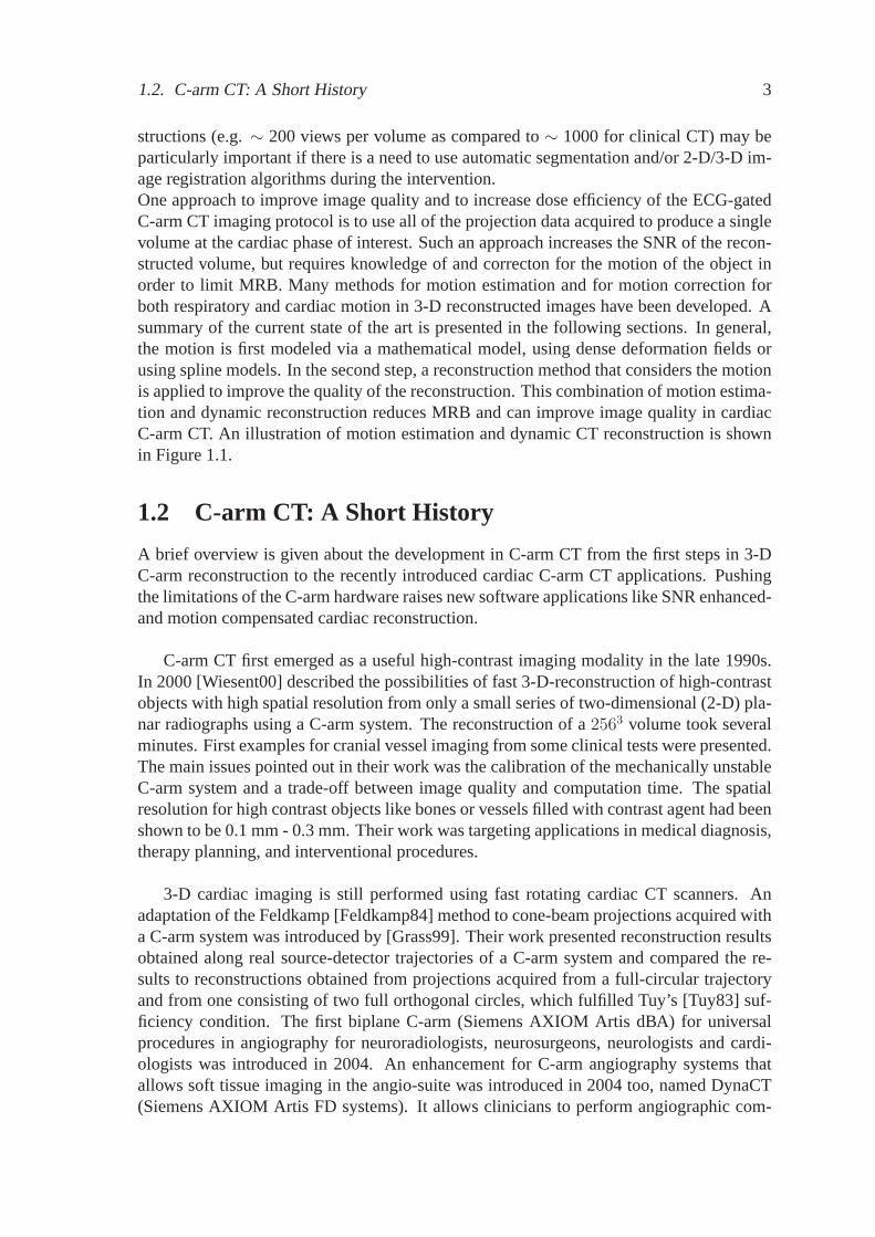
been adapted to the much slower rotational speed of C-arm CT. Motion of the heart is con-sidered in the reconstruction process by retrospective ECG-gating using only projectionsacquired at a similar heart phase.In 2007, a multi-axis system based on robotic technology was introduced. This systemallows a very flexible and fast positioning of the C-arm. Furthermore it has potential forhigher speed and accuracy of a rotational run and it allows DynaCT cardiac acquisition inhead side or lateral position. Examples of a multi-axis, biplane and ceiling-mounted sys-tem are shown in Figure 1.2. The reconstruction of a2563 volume is nowadays a matter ofless than ten seconds.The development of a fast and flexible C-arm CT systems is a continuous process, wherefor cardiac applications the rotation speed, frame rate and field-of-view of the detectorare important parameters to improve image quality. One major benefit from such C-armsystems is the integration of the 3-D and 2-D imaging technique into the interventionalworkflow. Thus the patient does not have to be moved to another modality/room duringthe procedure. However, the benefit of free access to the patient and the system, limits therotation speed. This is a necessary security issue for the patient. The hardware of the tothe C-arm connected workstation plays an important role as well. The acquired imagesare transfered to the workstation, where the reconstruction takes place. State-of-the-artworkstations perform for example Feldkamp reconstructions using graphics card hardwareacceleration like Compute Unified Device Architecture (CUDA) in less than4s for a2563

volume. A fast reconstruction is the basis for further post-processing steps like motionestimation based on a time resolved volume series.

Figure 1.2: From left to right: multi-axis system based on robotictechnology, Artis zeebiplane system enables biplane acquisition with up to 60 f/s, ceiling-mounted system. Incourtesy of Siemens AG, Healthcare Sector, source: www.siemens.com/artis-zee.

1.3 Related Work

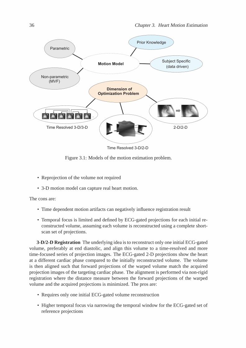
The focus of this thesis lies on the application of a combined motion estimation and dy-namic CT reconstruction. Both span a huge field of applications, where the motion esti-mation provides valuable information about the mechanical motion of the heart that canbe used for further analysis of the heart or used as prior knowledge for motion compen-sated CT reconstruction. The motion estimation can be grouped into approaches usinga parametrized motion model, based on prior knowledge or data driven considering thesubjects specific heart or even a combination of both. The dynamic CT reconstruction ofmoving objects like the heart is a topic that became more and more of interest over the lastyears. The theory of filtered backprojection reconstruction for static objects is well un-


derstood. Active research areas are still the exact reconstruction, deriving formulas wheretheoretically the object can be reconstructed exact, given a specific scan trajectory of theC-arm system. Furthermore the reconstruction of objects, scanned only by a limited viewangle, less than180 degrees, is still a research issue. Reconstruction problems of objectsthat are larger than the detector and thus are not captured completely in the projections- named truncation - are in the focus of many developers. Both issues can cause strongartifacts in the reconstructed image. In extension to theses issues, the heart moves duringthe scan. The temporal sampling of the acquired X-ray images is still quite sparse for aheart motion due to hardware limitations, compared to cardiac CT. Additionally to furtherhardware improvements the image quality is improved by image processing methods asdiscussed in the following. The theory of dynamic CT reconstruction is still under devel-opment and addressed by many researchers.

Thesis Work - Themethods introduced in this thesis are targeting the issues of temporalunder-sampling and improvement in image quality in terms of signal-to-noise. As a re-sult of ECG-gated reconstruction methods, not all acquired data is considered during thereconstruction. However, motion correction methods provide the tool for improved signal-to-noise and reduced motion blurring. Furthermore, theoretical considerations of dynamicfiltered backprojection and dynamic algebraic reconstruction are presented. The motionmodels for the dynamic CT reconstruction are derived in time resolved non-rigid 3-D/3-Dand 3-D/2-D registration.

The presented section on related work is basically organized according to the methods ofmotion estimation and dynamic reconstruction as well as resulting applications of SNRenhancing reconstruction methods.

1.3.1 Motion Model Estimation

Before deriving a heart motion model that provides the desired information for a mo-tion corrected reconstruction, the engineer has to decide if a parametric or non-parametricmodel is used. To increase robustness, the model can be designed in combination with priorknowledge of the model parameters about the heart motion pattern. Limiting the degreesof freedom of the motion model simplifies the optimization of the fitting process, however,to the cost of flexibility and thus individuality of the subject specific motion. Another im-portant question is the data that is used for the model fitting. For a good assessment of theoptions that arise during the design of a motion model, it is crucial to understand the de-sign options of the objective function and their qualities. We can for example fit the modelto a time series of ECG-gated initial volume reconstructions or directly to the measuredprojection data. In our work we constrain the heart model to be defined in 3-D plus thetemporal parameter. Motion modeling in the projection space lies not in the scope of thisthesis, since it cannot capture the real heart motion due to ambiguities. The options canbriefly itemized by:

• parametrized

• dense deformation field

• 4-D model that is fitted to a time resolved set of 2-D projection images

1.3. Related Work 7

• 4-D model that is fitted to several time resolved initial 3-D reconstructions

• any combination of the above mentioned plus optional prior knowledge about themotion pattern (e.g. averaged heart beat)

4-D Motion Estimation

In [Kalmoun07] a 3-D optical flow computation is proposed using a parallel variationalmulti-grid scheme that is considered to compute 3-D optical flow computation in real time.First experimental results using simulated data of a simplified cardiac model are presentedand the proposed variational multi-grid based on Galerkin discretization is compared toa Gauss-Seidel method. Here the Galerkin discretization outperforms the Gauss-Seidelmethod in a numerical simulation, however experiments based on motion blurred in-vivodata is not presented.A comprehensive review of variational non-rigid registration can be found in[Hermosillo02PhD], including details of distance measures such as sum of squared differ-ences, correlation based measures and mutual information as well as smoothness regular-izations for the deformation. Most of the registration algorithms proposed in the literatureprovide a non-symmetric motion estimation. The motion is computed starting from thefixed object (reference) towards the moving object (template). However, as introducedby [Han07], a symmetric motion estimation that provides a bijective mapping between thealigned volumes is desired. Han introduced a regularized Mumford-Shah Model that pro-vides a one-to-one edge matching of the aligned objects. Therefore no spatial regriddingof the dense deformation field is required to transform the volume to another cardiac phasein both time directions. However, as shown in [Han07] a bijective mapping is computa-tionally more expensive and it is not required for our application.A general review of 3-D modeling for functional analysis of cardiac images in differentmodalities is given by [Frangi01TMI]. A 4-D image registration method for consistent es-timation of cardiac motion from MRI image sequences was proposed by [Shen05]. Withinthis 4-D registration framework, all 3-D cardiac images obtained at different time-pointsare registered simultaneously and the motion estimation is forced to be spatiotemporallysmooth. This smoothness constraint overcomes the potential limitations of those methodsthat estimate cardiac deformation sequentially from one frame to another instead of treat-ing the entire set of images as a 4-D volume.[Taguchi06MIC] estimates the 2-D components of the MVF from a time sequence of 2-D cardiac CT slices. First, two image frames per heart beat (cycle) obtained at phaseswith slow motion (i.e., mid-diastole and end-systole) are reconstructed. Then, nodes arecoarsely placed inside the reconstructed 2-D slices and the temporal motion of each node ismodeled by B-splines. The proposed cost function consists of 3 terms: mean-squared-errorvia block-matching and smoothness constraints in space and time. The time-dependent 2-Dcomponents of the motion vector field (MVF) is estimated by minimizing the cost functionusing Powell’s estimation method.[Taguchi06SPIE] have also proposed an iterative approach repeating the following foursteps until the difference between two projection data sets falls below a certain criterion:1) estimate or update the cardiac motion vectors, 2) reconstructe the time-resolved 4-Ddynamic image volume using the motion vectors, 3) calculate forward projections from thecurrent 4-D images, and 4) compare them with the measured projection data.


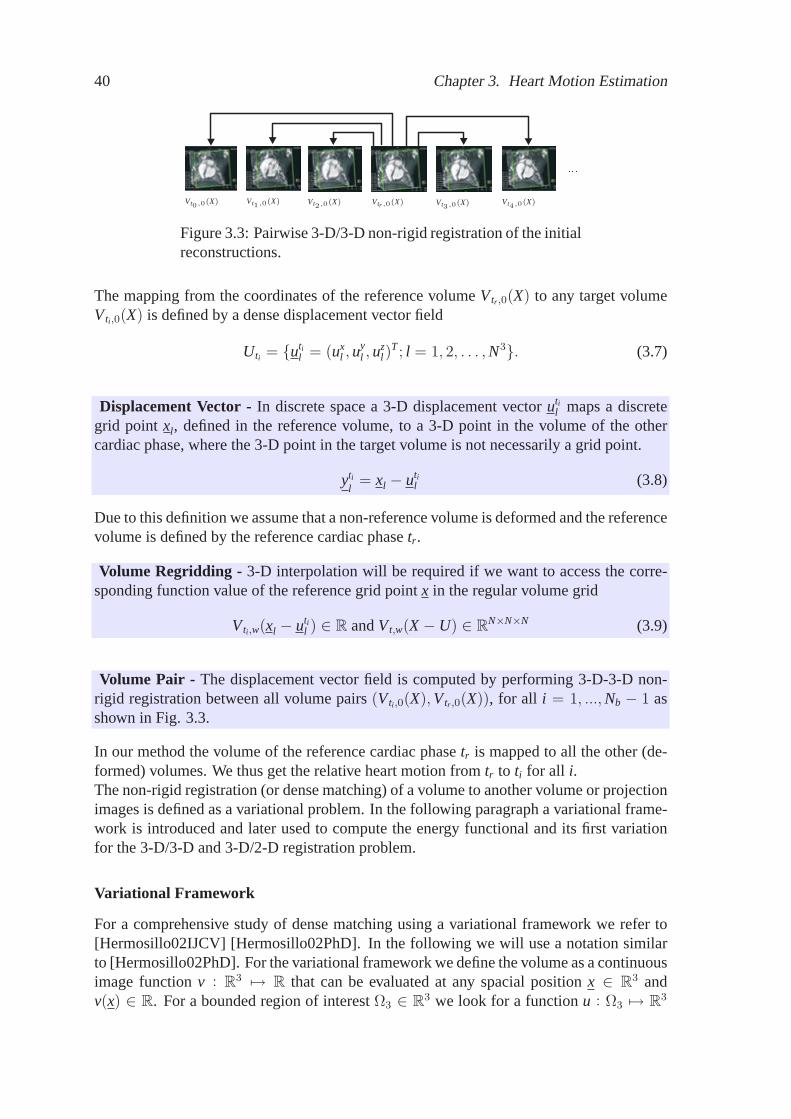
We choose a fast and parallel 3-D/3-D non-rigid multi-level registration method to dealwith larger deformations. The registration of volumes at different temporal positions donot depend on each other and thus error propagation over time is avoided. No prior knowl-edge for motion modeling is used, providing a purely subject-specific motion estimation sothat the anatomical structure of contrast-filled ventricles can be optimally aligned. This isespecially important for dynamic CT reconstruction of an individual subject. Initial stud-ies - presented in this thesis - using animal models have shown that a 4-D MVF can bederived for this application by computation of a subject-specific series of 3-D MVFs usinga variational non-rigid registration approach. The estimation of the MVFs is based on atime series of ECG-gated FDK reconstructions.

3-D/2-D Motion Estimation

An alternative approach for motion estimation to a time resolved 3-D/3-D approach is toalign a 3-D volume of a specific cardiac phase to few time resolved X-ray images of othercardiac phases. The major difference to the 3-D/3-D approach is that only one 3-D volumeis required and the registration process takes the original measured projection images - asreference - into account. The gain is that the projections are not disturbed by motion andother artifacts as observed in a 3-D reconstruction. Many 2-D/3-D registration methodsare proposed in literature. According to the distance measure, common methods can beroughly classified into feature-, intensity–based or statistical. Feature–based approachesmake use of landmarks (fiducial or natural) or other anatomical features to match images.Furthermore, most of the algorithms assume a rigid motion model such that degrees-of-freedom are reduced and the alignment of the volume to the set of projections can beexpected to be more robust. Our intention is the 4-D estimation of the heart motion. Mostof the published methods are targeting for example patient localization using about twoor even only one reference projection. Here, we give a generalized overview of relatingmethods, even if they are targeting a slight different application than the heart motion esti-mation, but all provide a 3-D to 2-D alignment method.For example, [Gueziec99] use surface features to align CT volume with fluoroscopy X-ray. [Feldmar94] presented a unified framework for registration of curves and surfaces.[Hamadeh95] extended Feldmar’s method by combining segmentation result of X-ray im-ages. Intensity–based registration measures the similarity of intensity directly. Thus,no feature extraction is required and the whole registration procedure can be automated.E.g., [Weese97] presented an intensity–based method for 2-D/3-D registration. [Fleute99]introduced an algorithm for reconstruction of 3-D shapes using a few X-ray views from aC-arm and a statistical model. They proposed to build the 3-D shape of the patient bonesor organs intra-operatively by deforming a statistical 3-D model to the contours segmentedon the few X-ray views. Fitting the model to the contours is achieved by using a gener-alization of the Iterative Closest Point Algorithm (ICP) to non-rigid 3-D/2-D registrationin application to surgical planning on 3-D images. [LaRose01] investigate real time itera-tive X-ray/CT registration techniques. [Zollei01] employ mutual information as similaritymeasure and a stochastic gradient ascent approach as optimization procedure in registrationproblems. [Yao03] proposed an affine 2-D/3-D registration method based on a statisticalmodel. [Jonic01] introduced a multi-resolution spline-based 2-D/3-D alignment of CT vol-ume and C-arm images for computer-assisted surgery.

1.3. Related Work 9

Most of the prior work focused on parameterized transformation, such as rigid or affinetransformation, i.e., the spatial transforms are defined by a set of parameters. However,in many clinic applications, it is more reasonable to describe the spatial transformationswith a non–parameterized model, i.e., the displacement field. For heart motion estimationwe introduce in this thesis a non-parametric motion model that is capable to describe thefull complexity of the heart motion in 3-D over time. The method is based on variationalcalculus and the robustness depends among other things on the number of time resolvedX-ray images that build the reference for the objective function. The similarity measure isprovided as statistical- and mono-modal measure.

1.3.2 Dynamic CT Reconstruction

Many motion correction methods for respiratory and cardiac motion have been proposedin the literature. Most of the methods consist of two steps. First, the motion is modeledvia a mathematical model, dense deformation fields, or spline models. Second, a recon-struction method incorporates the motion during reconstruction. Here one can distinguishbetween correcting the motion in the projection space or in the image space of the recon-structed volume or slice. In addition, there are different classes of object motion, such aslinear, affine, ray-affine or generalized non-rigid motion. Furthermore, the methods can begrouped into analytical methods that include filtering and iterative methods with no explicitfiltering process. Exact motion correction methods build probably the minority under thevariety of dynamic CT methods. Most of the methods are approximate, even in case theideal motion model is known. The methods can be briefly structured in:

• analytical method,

• iterative: algebraic reconstruction, statistical methods,

• motion model assumption: affine, ray-affine/linear or arbitrary non-rigid,

• filtering: projection space, after backprojection,

• parallel, fan-beam or cone-beam,

• exact or approximative.

Analytical Methods

[Roux04] presented an exact reconstruction method in 2-D dynamic CT (parallel and fan-beam geometry) that allows the compensation of time-dependent affine deformations. It isassumed that the motion parameters are known. The exact reconstruction method is basedon rebinning or sequential FBP. Results are presented using simulated data. Desbat, Rouxand Grangeat presented in [Desbat07TMI] a general work for 2-D+t dynamic tomography(parallel and fan-beam geometry) and also proposed a generalization to 3-D cone-beam;their scheme compensates analytically within filtered backprojection for object deforma-tions that are affine in time and along a line (ray). Generally they considered the class ofdeformations that transformed only a parallel projection geometry into an other parallelprojection geometry, or a divergent projection geometry into an other divergent projection


geometry. They showed that these deformations can be efficiently and analytically com-pensated with weighting and rebinning within each projection.[Taguchi07F3D], [Taguchi08TMI] introduced a method for motion compensated recon-struction using derivative backprojection filtering that corrects for locally affine transfor-mations. The proposed method allowed to reconstruct images from projections over aboutone motion cycle, resulting in reduced image noise level down to 40 percent of the cur-rent level. [Li06PMB] presented a first version of motion compensated reconstruction.They used a time-dependent transformation of 3-D filtered backprojections to incorporatea patient-specific motion model, and extended the algorithm to 3-D for cone-beam CT.It has also been shown that given a motion field of a dynamic (non-rigid) moving object, amotion corrected (dynamic) FDK-like reconstruction can be performed ( [Schäfer06TMI],[Prümmer06MIC], [Prümmer09TMI]). The dynamic reconstruction is performed by dy-namically adapting the geometry used for filtered backprojection according to the MVFs.These methods can deal with arbitrary non-rigid cardiac motion, but the filtering and re-dundancy weighting is still approximate.[King06] introduced a weighted backprojection filtration algorithm for the reconstructionof motion-contaminated data. Their idea was a weighted backprojection filtration usingdata redundancy. The method is capable of reconstructing region-of-interest images fromreduced-scan fan-beam data, which have less data than the short-scan data required to re-construct the entire field of view. Second, this algorithm reconstructs ROI images from thetruncated data.

Iterative Methods

[Blondel06TMI] introduced a method that consists of three steps: 1) 3-D reconstructionof coronary artery centerlines, including respiratory motion compensation, 2) computationof the 4-D coronary artery motion, and 3) 3-D tomographic reconstruction of coronary ar-teries, with compensation for respiratory and cardiac motion. A dynamic projector modelcombined with an iterative ART method is used for the motion compensated reconstruction.Pack and Noo introduced in [Pack04] a dynamic CT reconstruction with known motionfield using an ART-like method. They introduced an iterative ART algorithm with a pro-jection operator and a backprojection operator that are matched to ensure fast convergenceand are both computationally efficient. The projectors are adapted to the continuous mo-tion field. Results using computer-simulated data are presented. A method for evaluatingthe sufficiency of the data and predicting image quality of the reconstruction based on boththe acquired angular range and the known motion field is proposed.Desbat and Clackdoyle [Desbat07EMBS] published algebraic and analytic approaches fordynamic tomography. They presented a framework of dynamic tomography for both al-gebraic and analytic approaches. Results using a realistic digital phantom of the thoraxare provided. They show a comparison of a heuristic compensation of the motion duringthe backprojection (Dynamic Feldkamp) to dynamic SART. Their work concludes that dy-namic SART is identical to SART when the projector models the motion properly.To perform a dynamic reconstruction, assuming a non-rigid motion model, a projectorthat models the object motion by adapting the projection geometry is required. A motion-compensated iterative cone-beam CT image reconstruction method with adapted blobs as

1.3. Related Work 11

basis functions was introduced by [Isola08] [Pack04]. An efficient method to calculate theline integral through the adapted blobs is proposed. It solves the problem, how to com-pensate for the divergence in the motion vector field on a grid of basis functions. Isolapresents also a comparison between a motion-compensated filtered backprojection and theproposed iterative methods using adapted blobs.

1.3.3 SNR Enhanced Reconstruction

An approach for respiratory motion compensation and SNR enhancement was introducedby [Li05MP]. The 3-D CT images at different phases are registered to the same phase via adeformable model. A regularization term combining temporal and spatial neighbors is pro-posed and thus dose reduction can be achieved. A second method [Li07MP], introduced for4-D cone-beam CT (4DCBCT), correlates the data in different respiratory phase bins andintegrates the internal respiratory motion into the 4DCBCT reconstruction. Each filteredbackprojection is deformed by a time-dependent transformation to correct for motion. Thisapproach is similar to our method, but we address the problem of cardiac motion, whichis more complex because it is highly variable in both temporal and spatial domains. Theless complex respiratory motion can be regularized globally, and image artifacts shouldnot significantly corrupt the motion estimate. The SNR enhancement introduced by T. Liet al. increases blurring when edges of different phases do not match perfectly, as is ex-pected to be the case for artifact-prone cardiac reconstruction. We introduce in this thesisweighting schemes that addresses this problem [Prümmer07BVM]. The improvement inimage quality via the integration of data from different respiratory or cardiac phases tothe desired phase is limited by the temporal resolution of each single reconstructed phase.We therefore chose an approach that aligns each acquired projection image to the desiredphase. The projection data is gated into several subsets, where each subset provides datafor a short-scan. Each motion corrected short-scan contributes according to the expected orestimated confidence of the corrected data to the resulting reconstruction using weightingschemes.

1.3.4 Discussion

Iterative motion estimation and reconstruction methods (eg.[Taguchi06SPIE]) are timeconsuming. This is especially true when the energy functional contains a combinationof 3-D/4-D image data and 2-D projection images. Methods where the motion is onlyestimated in 2-D projection space are limited because 3-D motion cannot be uniquely mea-sured in sinogram space. Furthermore cardiac motion lies in the generalized deformationclass of non-rigid motion. The introduced motion correction method by [Desbat07TMI]is currently the most powerfulexact methodin terms of degrees of freedom of the objectmotion, ray-affine motion.In this work we use non-iterative, combined motion estimation and correction in 4-D usingan approximate, but fast dynamic filtered backprojection approach. The motion correc-tion method is based on the work of [Li06PMB] and has been optimized for the recentlyintroduced multi-sweep C-arm acquisition protocol [Lauritsch06TMI]). Iterative dynamicmethods are more powerful in terms of exact reconstruction, assuming an ideal motionmodel. This is justified in the implicit filter process of the iterative forward and backpro-


jection. Thus no explicit filter has to be derived - like in FBP - what can be a complexand time consuming process if we are faced with a shift-variant system in case of arbitrarymotion.

1.4 Contributions to Cardiac C-arm CT

In this thesis, we present new work demonstrating SNR improvement using a subject spe-cific estimated dense deformation field in combination with a modified FDK algorithm foruse with the new ECG-gated C-arm CT imaging protocol. We follow the two-step processas outlined above, with some key refinements. First, the motion vector field (MVF) is cal-culated between the reconstructed cardiac phases and a reference phase, using a multi-level3-D/3-D registration approach that has been run-time optimized to provide a fast estimateof the MVF suitable for use in the clinic. We then concatenate these dense deformationfields to generate a time-continuous 4-D MVF using interpolation between cardiac phases,so that the trajectory of each voxel throughout the whole cardiac cycle is known. To recon-struct the corrected volume, each projection is backprojected along a curved path, with thepath determined by the voxel being reconstructed, the phase at which the projection wasacquired, and the estimated MVF. We carry out motion correction in the projection space,which maximizes the resulting image quality for a given accuracy of the MVF.

Since subject-specific heart motion encoded in the MVF can only be estimated approx-imately and non-rigid heart motion cannot be corrected exactly by current dynamic FDK-like algorithms, a trade-off exists between spatial resolution and SNR, depending on theprojection data used for reconstruction. In this work we present two new weighting meth-ods to combine all of the acquired projection data from a multi-sweep protocol (publishedby [Lauritsch06TMI]) into a single reconstructed volume: weighting by cardiac phase vari-ance and weighting by intensity variance. The resulting motion-corrected image quality iscompared to uncorrected FDK-like reconstructions and also compared to the current state-of-the-art ECG-gated Feldkamp reconstruction. Image quality is evaluated and comparedby measuring the edge response function versus SNR for all of the reconstruction methods.In summary the major contributions for cardiac C-arm CT are:

• combined motion estimation and correction

• SNR enhancement

• further image quality improvements.

Beside this major contributions to cardiac C-arm CT many theoretical aspects aboutdynamic CT and motion estimation are investigated and derived in this thesis. These fun-damental considerations extent the understanding of filtered backprojection methods aswell as iterative reconstruction in case of the moving heart in application to cardiac C-armCT. The resulting image quality of the dynamic FDK-like algorithm and the SNR enhanc-ing weighting schemes is evaluated using several porcine models in combination with asubject specific motion estimation under real clinical conditions. The thesis contributesalso to the motion model estimation using a novel and flexible non-rigid 3-D/2-D regis-tration algorithm that is especially evaluated using the NCAT [Segars03] heart phantom,

1.5. Heart Anatomy and Cardiac Cycle 13

embedded into the common multi-segment C-arm CT acquisition protocol. The non-rigid3-D/2-D registration algorithm has potential for further applications in cardiac C-arm CTlike interventional guidance, where pre-op CT data can be aligned to intra-interventionalacquired X-ray images using a C-arm. Other applications can be in the field of respiratorymotion estimation.Theoretical considerations of the Fourier-slice theorem in combination with different mo-tion models as well as dynamic filtered backprojection are presented and derived. Thisallows to understand the limits of filtered backprojection methods, when the point-spread-function of a combined forward and backprojection becomes shift-variant. In these casesno efficient inversion method to reconstruct the object exact is known, assuming an idealmotion model. Further the class of dynamic ART reconstruction methods is introducedusing a dynamic projector model similar to [Pack04] and in addition a method that is basedon a dynamic object geometry in combination with a fast static projector is presented. Themethods are compared to each other.

1.5 Heart Anatomy and Cardiac Cycle

1.5.1 Anatomy

The following brief description of the heart is based on the work of Henry Gray „Anatomyof the Human Body“ (1821 to 1865). Only anatomical details, as relevant for this work,are cited here. Further details can be found in the public domain online book [Gray18] ofHenry Gray.

„The septasubdivides the heart into a left and right half. Each half is subdivided intotwo cavities, the upper atrium and the lower ventricle (see Figure 1.3). The right and leftatria and right and left ventricles build the four chambers.“

„The right atrium is larger than the left, but its walls are somewhat thinner, measur-ing about 2 mm. Its cavity is capable of containing about57cc. It consists of two parts: aprincipal cavity, or sinus venarum, situated posteriorly, and an anterior, smaller portion,the auricula.“

„The right ventricle is triangular in form, and extends from the right atrium to nearthe apex of the heart. Its anterosuperior surface is rounded and convex, and forms thelarger part of the sternocostal surface of the heart. Its under surface is flattened, restsupon the diaphragm, and forms a small part of the diaphragmatic surface of the heart. Itsposterior wall is formed by the ventricular septum, which bulges into the right ventricle,so that a transverse section of the cavity presents a semilunar outline.“

„The left atrium is rather smaller than the right, but its walls are thicker, measuringabout 3 mm. It consists, like the right, of two parts, a principal cavity and an auricula.“

„The left ventricle is longer and more conical in shape than the right, and on trans-verse section its concavity presents an oval or nearly circular outline. It forms a smallpart of the sternocostal surface and a considerable part of the diaphragmatic surface of


the heart. It also forms the apex of the heart. Its walls are about three times as thick asthose of the right ventricle.“

„The coronary sinus opens into the atrium, between the orifice of the inferior venacava and the atrioventricular opening. It returns blood from the substance of the heart andis protected by a semicircular valve, the valve of the coronary sinus.’

Inferiorvena cava

Membranousseptum

Musculipectinati

Left auricula

Aortic valve

Papillarymuscles

Anterior papillary muscle

Figure 1.3: Left: Section of the heart showing the ventricularseptum. Right: Interior ofleft side of heart (by courtesy of Henry Gray 1825 to 1861, Anatomy of the Human Body1918. Source: [Gray18])

1.5.2 Cardiac Cycle

The understanding of the cardiac cycle, specifically the mechanic motion is crucial forfurther approaches in motion estimation and dynamic CT reconstruction. To provide somebasic knowledge about the cardiac cycle, as relevant for this thesis, we cite briefly thedescription by Henry Gray [Gray18]: „By the contractions of the heart the blood is pumpedthrough the arteries to all parts of the body. These contractions occur regularly and at therate of about seventy per minute. Each wave of contraction or period of activity is followedby a period of rest, the two periods constituting what is known as a cardiac cycle. Eachcardiac cycle consists of three phases, which succeed each other as follows: (1) a shortsimultaneous contraction of both atria, termed the atrial systole, followed, lowed, after aslight pause, by (2) a simultaneous, but more prolonged, contraction of both ventricles,named the ventricular systole, and (3) a period of rest, during which the whole heart isrelaxed. The atrial contraction commences around the venous openings, and sweeping overthe atria forces their contents through the atrioventricular openings into the ventricles,regurgitation into the veins being prevented by the contraction of their muscular coats.When the ventricles contract, the tricuspid and bicuspid valves are closed, and preventthe passage of the blood back into the atria. The musculi papillares at the same time are

1.6. Document Overview 15

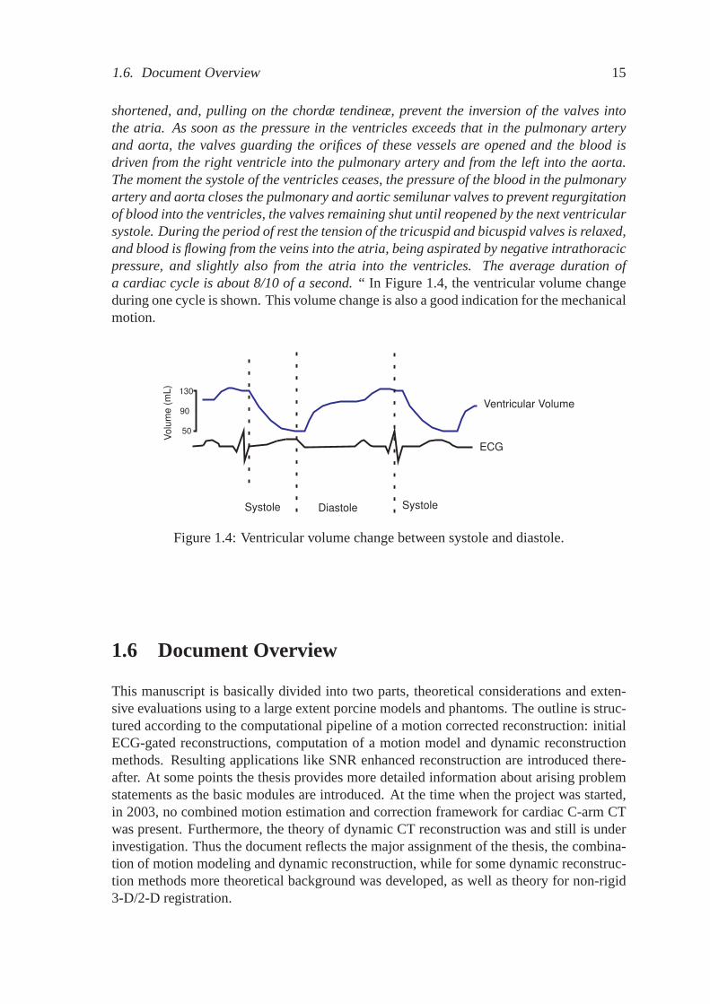
shortened, and, pulling on the chordæ tendineæ, prevent the inversion of the valves intothe atria. As soon as the pressure in the ventricles exceeds that in the pulmonary arteryand aorta, the valves guarding the orifices of these vessels are opened and the blood isdriven from the right ventricle into the pulmonary artery and from the left into the aorta.The moment the systole of the ventricles ceases, the pressure of the blood in the pulmonaryartery and aorta closes the pulmonary and aortic semilunar valves to prevent regurgitationof blood into the ventricles, the valves remaining shut until reopened by the next ventricularsystole. During the period of rest the tension of the tricuspid and bicuspid valves is relaxed,and blood is flowing from the veins into the atria, being aspirated by negative intrathoracicpressure, and slightly also from the atria into the ventricles. The average duration ofa cardiac cycle is about 8/10 of a second.“ In Figure 1.4, the ventricular volume changeduring one cycle is shown. This volume change is also a good indication for the mechanicalmotion.

Ventricular Volume

DiastoleSystole Systole

Volu

me

(mL)

50

130

90

ECG

Figure1.4: Ventricular volume change between systole and diastole.

1.6 Document Overview

This manuscript is basically divided into two parts, theoretical considerations and exten-sive evaluations using to a large extent porcine models and phantoms. The outline is struc-tured according to the computational pipeline of a motion corrected reconstruction: initialECG-gated reconstructions, computation of a motion model and dynamic reconstructionmethods. Resulting applications like SNR enhanced reconstruction are introduced there-after. At some points the thesis provides more detailed information about arising problemstatements as the basic modules are introduced. At the time when the project was started,in 2003, no combined motion estimation and correction framework for cardiac C-arm CTwas present. Furthermore, the theory of dynamic CT reconstruction was and still is underinvestigation. Thus the document reflects the major assignment of the thesis, the combina-tion of motion modeling and dynamic reconstruction, while for some dynamic reconstruc-tion methods more theoretical background was developed, as well as theory for non-rigid3-D/2-D registration.


Chapter 1

A state of the art overview and clinical applications for cardiac C-arm CT are presentedand motivated in the first chapter. Necessary background knowledge about cardiac inter-ventions and anatomy of the heart is provided as well.

Chapter 2

The chapter starts with the brief introduction of the meanwhile established cardiac C-armCT imaging technique, explaining multi-segment acquisition protocols and ECG-gated re-construction in chapter two. Arising problems of gating techniques like a relative or ab-solute cardiac phase/time, as well as image-based gating, is presented. Calibration issuesthat come along with the new multi-segment acquisition protocol are briefly considered.

Chapter 3

Methods to estimate the subjects specific motion model are introduced in chapter three.First, the derivation of a dense motion vector field is presented, based on a time series ofinitial ECG-gated reconstructions. Standard methods of non-rigid 3-D/3-D registration areapplied and sampling, interpolation and pre-processing issues are addressed. The secondpart of chapter three provides several techniques to derive a motion model based on onesingle initial 3-D reconstruction that is aligned to a time resolved subset of projectionimages. A mono- and multi-modal non-rigid 3-D/2-D registration approach is derivedtheoretically using a variational framework and approximative methods are presented aswell.

Chapter 4

Assuming a known motion model as derived in chapter three, some fundamental theoret-ical background for dynamic 2-D parallel-beam filtered backprojection is developed. TheFourier slice theorem is discussed introducing several different motion models. An exten-sion to dynamic 3-D cone-beam reconstruction is introduced as a Feldkamp-like modifica-tion that is capable to approximatively correct motion. Furthermore, algebraic reconstruc-tion of dynamic objects is introduced afterwards. A dynamic projector model that modelsthe object motion and in analogy a solution using a dynamic object grid and a static pro-jector is introduced.

Chapter 5

As an application of the resulting motion model of chapter three, combined with algo-rithms for dynamic CT reconstruction of chapter four, several SNR enhancing reconstruc-tion techniques are stated in chapter five. Here, the focus lies on the trade-off betweenmotion related blurring as a result of approximative motion correction and signal-to-noiseratio using all acquired projections.


Chapter 6

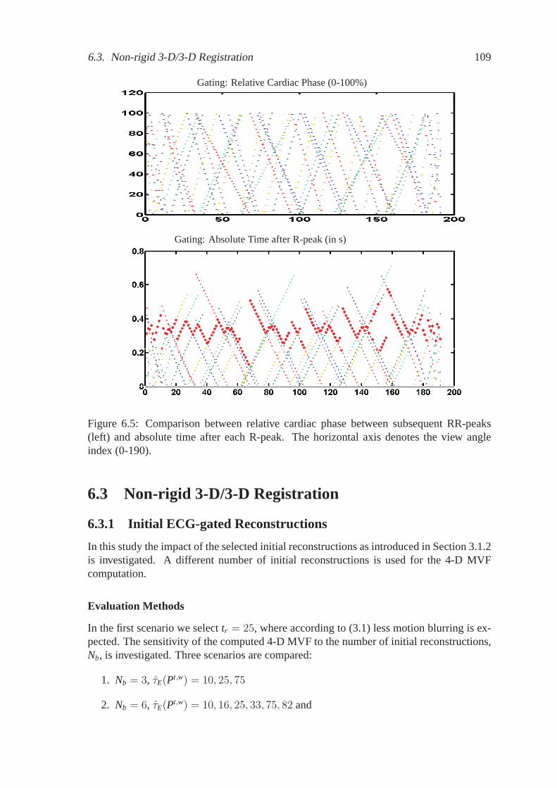
The second major part of the manuscript starts with chapter six. The introduced meth-ods for motion estimation are evaluated using a plastic and porcine models. The impactof the number and temporal distribution of the initial 3-D reconstructions is investigated.Gating methods are compared using an animal model and the impact of the temporal inter-polation method and temporal regularization of the dense deformation field is discussed.Furthermore a framework to measure the accuracy of the computed 4-D MVF model usingultrasound is introduced and applied. The 4-D motion of a physical plastic phantom iscomputed and assessed. Several porcine models provide a fundamental investigation aboutthe performance of a 3-D/3-D non-rigid registration approach for a motion model deriva-tion. The capacity of the 3-D/2-D non-rigid registration approach is demonstrated usingthe NCAT phantom [Segars03].

Chapter 7

Using the derived motion models from chapter six, the performance of motion correctedreconstruction using dynamic filtered backprojection is evaluated. Several SNR enhancingreconstruction methods are compared to each other using a plastic phantom and an animalmodel. Important issues about sampling in dynamic filtered backprojection are addressedas well. Selected cases of dynamic FBP in combination with a previously derived motionmodel are presented. For example the case of a single-sweep correction assuming a knownMVF and different multi-segment scan protocols like4 × 4s and6 × 4s are discussed incombination with motion correction (see Figure 1.1).

Chapter 8

The flexibility of algebraic reconstruction in combination with shift-variant filter systems,as given in case of non-rigid heart motion, is discussed and simulated. The resulting systemmatrix and its structure, depending on the expected motion model like affine, ray-linear orarbitrary non-rigid motion, is investigated. Using a from an animal model derived 4-DMVF, the resulting point-spread-function and the condition of the resulting system matrixis evaluated. Furthermore, the performance of a dynamic projector model vs. a dynamicobject grid is investigated.

Chapter 9

A summary and collection of problem statements that arised during the development andinvestigation of the methods is completing the manuscript.



Theory„In theory, everything is possible.“


Chapter 2

Multi-segment Cardiac C-arm CT

Multi-segment cardiac C-arm CT has been adapted in 2006 from the multi-segment acqui-sition protocol as it is performed in cardiac CT reconstruction. One of the major differencesbetween cardiac C-arm CT and cardiac CT is the rotational speed of the X-ray source thatplays an important role in case of moving objects like the heart. Current CT scannerscan rotate360 degrees in less than350ms and thus provides a higher temporal resolutioncompared to C-arm CT. Lauritsch [Lauritsch06TMI] introduced an approach for cardiacimaging that takes advantage of recently improved contrast resolution and is based on in-travenous contrast injection. In C-arm CT, the scanner device cannot rotate360 degreecontinuously due to limitations by hardware like connection cables. Thus the detector andX-ray tube, mounted on a C-arm, rotate forth and back instead of unidirectional. A typicalscan protocol for one single forward sweep is the rotation about220 degree (also calledshort-scan) in about4s (see Figure 2.1). Thus we can expect about5 heart beats (HB)during one sweep assuming one cyclic beat takes about0.8s. This clearly depends on thecondition of the patient.

Figure 2.1: The image sequence (left to right) illustrates a singleC-arm rotation that cantake about4s and220 degrees of rotation. Source: Siemens Syngo C-arm model.

In this example we capture each0.8s the same motion state of the heart, but at a differ-ent angular position of the rotating device. A non-moving object can be reconstructed usingthe data of one single sweep (short-scan). In cardiac reconstruction, the utilizable amountof data drops to1/HB for a single C-arm sweep, if only gated data is used that representsthe heart in the same motion state. A common technique to determine the time dependentmotion state of the heart is to detect R-peaks (see Figure 2.4) in the ECG signal that isrecorded during the scan. It is assumed that the heart moves periodically and describes ineach period the same motion pattern. It is important to be aware of the fact that especiallypatients, which are in a less healthy condition, can have irregular beats and motion. In

21

22 Chapter 2. Multi-segment Cardiac C-arm CT

case of FDK reconstruction, the sparse angular sampled data of1/HB of a single sweepprovides not a sufficient amount of data for a good image quality. To increase the amountof data, available to reconstruct a specific cardiac phase, the multi-segment data acquisitiontechnique has been adapted from cardiac CT to cardiac C-arm CT. However, in contraryto cardiac CT, the C-arm rotates forth and back during the scan [Lauritsch06TMI]. TheC-arm device is triggered between the forward and backward sweeps such that acquiredprojection data of the different sweeps covers approximately the same cardiac phase, butdifferent view angles of a complete short-scan by triggering the targeting reconstructionphase (see Figure 2.5). This technique allows a retrospective gating of projection imagesfor a time resolved motion phase.

As stated in the introduction the focus of this thesis lies on the reconstruction of con-trasted ventricles using cardiac C-arm CT. In this section we introduce the acquisitionprotocol that is principally based on the work of [Lauritsch06TMI]. First, the acquisitionprotocol focusing on scan duration, contrast injection and breath-hold is introduced, sec-ond the cardiac phase identification is discussed and third the technique of retrospectivegating is presented.

2.1 Acquisition Protocol

2.1.1 Series of Alternating Forward and Backward Runs

The C-arm rotates in each single sweep aboutπ + 2 × fan-angle. The C-arm accelerates,achieves a constant angular speedωr and decelerates until it stops in about 4-5 seconds forthe full sweep. The acceleration and deceleration phase is short compared to the constantangular speed interval and thus will be neglected in the following considerations. Theangular position of the X-ray source is expressed asθs = ωr ta with the absolute sweeprotation timeta in seconds. The subindexs denotes the scanner while we will have anobject rotation as well later on.

Cardiac Phase -The cardiac phaset is defined by its position between R-peaks in theECG signal and it is measured in percent.

t ∈ [0, 100] (2.1)

The targeting reconstruction phase is denoted bytr ∈ [0, 100], with a temporal windowwidth ∆t ∈ [0, 100], centered attr ∈ [0, 100]. To cover a complementary angular rangeof the same cardiac phase in a subsequent sweep a start time offset between subsequentsweeps is applied. The number of forward and backward sweeps isNs. Lauritsch [Lau-ritsch06TMI] derived the start time offset formulatbj = 100−tEnd+2tr−100(j−1)/Ns. Theindex j (restricted to an even number of sweeps) denotes the current number of performedsweeps during the scan andtEnd is the heart phase of the first forward run(j = 1). Thustbjtells us the triggered time delay between each subsequent sweep such that an optimal com-plementary angular range of the same cardiac phase is scanned. Given a fixed delay timetbj , a resulting scan symmetry leads to several optimal reconstruction phasestr . A modulooperation keeps all cardiac phases between0 − 100 percent. The optimal reconstructionphasetr is setup before the scan. A reconstruction of other phases can lead to a decreased

2.1. Acquisition Protocol 23

temporal resolution. This multi-segment acquisition protocol allows a retrospective gatingfor a time resolved short-scan reconstruction. The resulting cardiac phase vs. view anglesampling is illustrated in Figure 2.5. The horizontal axis denotes the short-scan view po-sition of X-ray source and the vertical axis the relative cardiac phase between subsequentR-R peaks. The diagonal line pattern shows the resulting sampling of acquired projectionimages due to view angle and cardiac phase. For a short-scan reconstruction, the projec-tion images that lie close to the reference cardiac phase are gated. Further details about thegating technique will be explained later.

2.1.2 Scan Parameters

Further important scan parameters are among others breath-hold duration, X-ray dose, con-trast volume and dilution, overall acquisition time and image acquisition speed of the C-arm (frames

s ). There is a trade-off between the parameters: breath-hold duration, intravenousinjected contrast volume, X-ray dose and the number of sweeps and the rotation timeNs, ta.With increasingNs the expected temporal resolution is increasing assuming a constantta.However, this is limited by the expected breath-hold time and the overall injected contrastvolume. Furthermore the X-ray dose is increasing as well. It is important to provide a con-tinuous and homogeneous contrast flow during the scan to avoid contrast streaming. Theseparameters have all been evaluated and optimized during first clinical tests using animalmodels, since the interaction is quite complex for a pure theoretical developed. Specificscan parameters are provided in the evaluation chapters. The contrast injection starts sev-eral seconds before the first C-arm rotation begins. The scan parameters using exemplaryvalues can be summarized as:

• Breath-hold duration; acquisition time< 30s

• Intravenous injected contrast volume< 150ml, 3, 5ml/s

• Rotation speed and frame rate about60 frames/s

• Alternating forward and backward runs; ECG synchronized

• X-ray dose e.g.90kV/pulse, 1.2µGy/frame

• Single sweep rotation time4s≤ ta ≤ 6s

2.1.3 Practical Aspects

The multi-segment acquisition protocol raises some practical issues like the geometricalcalibration. Some comments about an extended calibration for multi-sweeps compared toa single C-arm sweep are given in the following. Furthermore we comment on contrastinjection and sparsity of time resolved data.

C-arm Calibration

The alternating series of forward and backward runs raises new calibration issues. In caseof a single sweep rotation the C-arm is calibrated for each single view angle index position.In the calibration step a3 × 4 homogeneous projection matrix is computed that projects a


homogeneous 3-D lattice position onto a homogeneous 2-D position on the detector. Thisprojection matrix is a composition of the extrinsic and intrinsic transformations that applyif a 3-D position is projected onto the 2-D detector. This technique has been establishedover the years and it is assumed that the C-arm is vibrating with a reproducible patternduring one single sweep. Thus for each single view position the homogeneous projectionmatrix is computed once during the calibration and later used for the reconstruction. Forthe extended multi-sweep protocol it can be expected that this vibration pattern differs fora forward and backward run. The general calibration issue, however, is beyond the scopeof this work and all evaluations as presented in this thesis have been done using the samecalibration for forward and backwards runs. It results from a single forward run calibration.During further refinement of the acquisition protocol as introduced by [Lauritsch06TMI],we investigate briefly how reasonable this assumption is.First investigations, in the year 2007, (see Figure 2.2) show that computing for each viewposition two homogeneous projection matrices, one for the forward sweep and one for thebackward sweep, can further improve the image quality. In Figure 2.2 two reconstructionsare compared. The calibration of the C-arm system was split into two parts. The rightcolumn shows a multiplanar reconstruction (MPR) and VRT (Volume Rendering Tech-nique) of a reconstruction, where the system is calibrated separately for a forward andbackward sweep. Due to the slightly different vibration patterns between a forward andbackward sweep, the projection images of the same object with the same projection angledo not match. Thus we introduce motion, caused by the C-arm position that furthermorecan cause artifacts in a gated reconstruction. Projection images from different forward andbackward runs are contributing to the gated reconstruction. As shown in Figure 2.2, arrow1, an artificial edge as shown in the left MPR is introduced in the soft tissue around therib due to calibration inaccuracy. Here no separated forward and backward run calibrationwas performed. The MPR and volume rendered image as shown in the right column isreconstructed using a separated calibration. One calibration run for a forward sweep andan additional calibration run for a backward sweep. Contrasted ventricles provide a highercontrast and are more homogeneous in case of a separated calibration, Figure 2.2 arrow2. The ventricles also appear brighter using the same windowing in the MPR and VRTrespectively. At the arrow position 3 (right column) we can see that the structure of vesselsis shown more clearly. The result presented here was the very first attempt for an improvedcalibration. Further investigations need to be done, however, this first example alreadyshows that a sweep specific calibration has potential for further improvement of the imagequality.

Contrast Injection

Neglecting the heart motion it is assumed that the contrast flow and dilution is homoge-neous in vessels and ventricles during the complete scan. This is an important constraintsince in case of violation the measured data is not consistent. The object that is recon-structed would change its density during the scan such that the attenuation inside the objectdiffers over time. For simplification in this thesis and focus on object motion, we assumethat contrast flow and dilution is homogeneous. In a clinical environment this assumptionmight be violated. The timing of the intravenous contrast injection as well as the flow isquite important to provide projection data that only differs in the motion state of the heart.

2.1. Acquisition Protocol 25

1 1

2 2

3 3

2 2

Figure 2.2: Comparison of reconstructions with different calibration.The left columnshows the reconstruction, where the C-arm system was calibrated only for forward sweeps.The right column shows a MPR and a VRT of a resulting reconstruction using a separatedcalibration for forward and backward sweeps.

Thus in a real world scenario we actually have to deal among other things with motion(cardiac and maybe respiratory) and density variations due to contrast flow. The observedX-ray intensity on the detector is the superimposed result of these effects. Thus the spatialvolume motion and change of densities cannot be distinguished. However, it is importantto be aware of this issue as illustrated in Figure 2.3. Especially during the projection imageacquisition of the first forward sweep and the last sweep it is more likely that contrast isstreaking inside the ventricles as shown in Figure 2.3.


Figure 2.3: Example of inhomogeneous contrast flow during a scan.The sequence fromtop to bottom shows the angular index 189, 191 and 193. In this case a strong contraststream is observed although only a small angular window of4× 0.8 degrees is scanned.

2.2. Cardiac Phase Identification 27

Sampling Considerations of the Data

To derive algorithms that can compensate the heart motion, a fundamental understandingof the temporal and angular sampling of the acquired data is mandatory. It is expectedthat motion-free imaging of the coronary arteries requires a temporal resolution of about50ms. Assuming an average heart beat duration of0.85s a temporal quantization of about50ms/850ms= 1/17 of a R-R peak would be desirable. This is just a numerical example,but it points out the sparsity of the measured data. SettingNs = 17 and the number ofprojections per sweep to200 we would acquire200 × 17 = 3400 projection images. Foreach of the200 view angles17 projections would be measured. Current plausible protocolsprovide(Ns = 4) × 200 = 800 projection images. This is only23, 5 percent of the de-sired data of this numerical example. This motivates reconstruction approaches that workwith temporally averaged data. In the following we will derive heart motion models thatare estimated subject specific. This requires the reconstruction of several different cardiacphases. For example five volumes are initially reconstructed. A full angular sampling isfocused and thus the data is averaged temporally to cover a full angular sampling for fil-tered backprojection reconstruction. Thus the heart motion model is based on temporallyaveraged data as well. The motion model is then applied during a motion compensatedreconstruction. Optional to a motion estimation and correction approach one can thinkabout interpolation of the projection images in the sinogram space. The sinogram spaceis 4-D. For one single cardiac phaset we have a discrete stack of about 200 2-D projec-tions and thus already three dimensions. Adding the temporal dimension we have to dealwith a 4-D problem for an interpolation approach. Along the view angle axis, the inter-polation method has to model the observed sinogram motion (including calibration issues)and along the temporal axis (for a specific view angle) one has to model the heart motion.However, considering the angular/temporal sampling of a4×4s multi-segment acquisition(see Figure 2.5) it is obvious that a 4-D sinogram interpolation method has to deal withhighly under-sampled data.

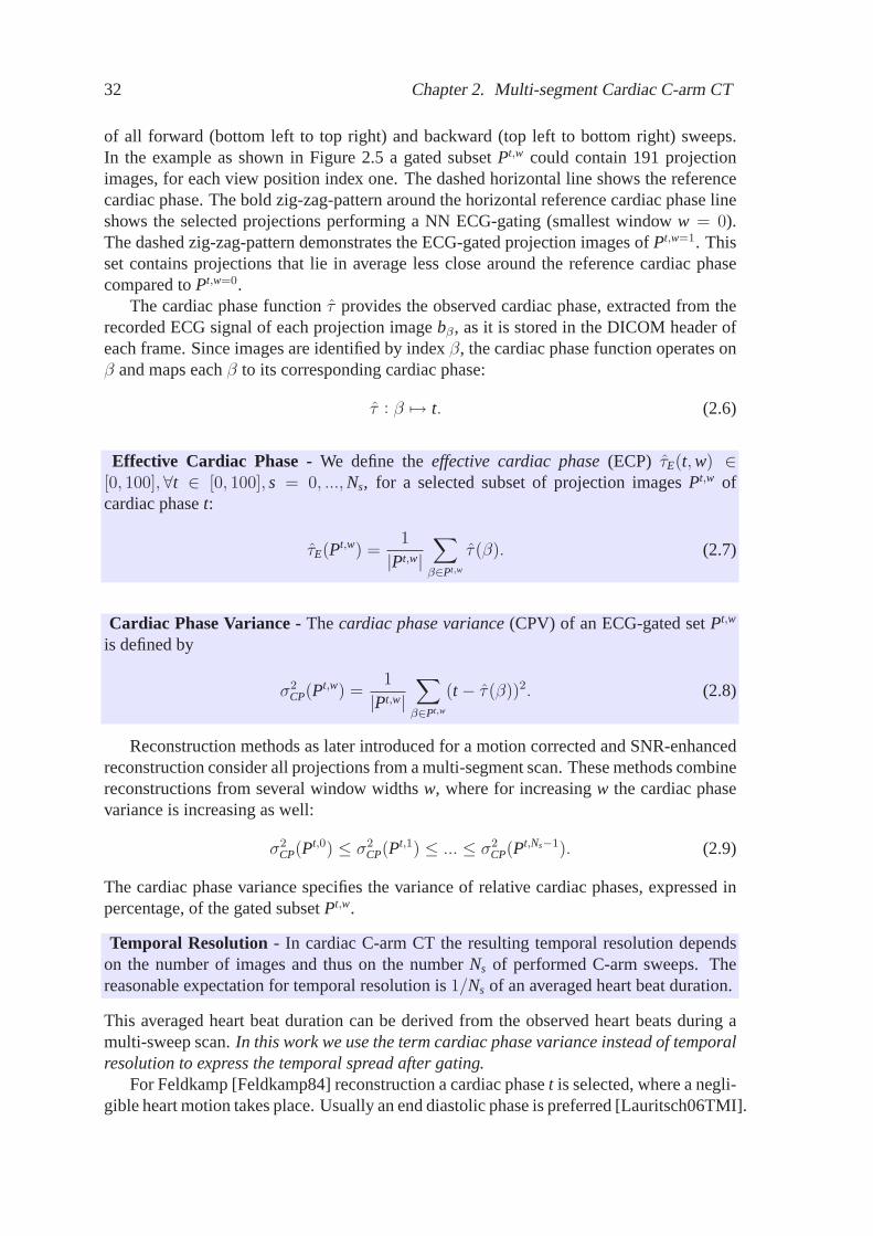
2.2 Cardiac Phase Identification

To reconstruct a time resolved cardiac image we need to assign a cardiac phase to eachprojection image. Then a subset out of all acquired projections can be gated, where eachimage in this subset shows the heart approximately at the same cardiac phase. The iden-tification of the corresponding cardiac phase of an image is usually done in percentagebetween two detected subsequent R-peaks in the ECG signal. In the following sections theelectrocardiogram is introduced. Furthermore the detection of R-peaks in the ECG signaland a technique to compute a relative cardiac phase is explained. As an alternative to therelative R-R peak phase, an absolute time gating method is presented. The heart motiondependency on the heart rate is discussed for a relative and absolute phase gating.

2.2.1 Electrocardiogram

An electrocardiogram is a recording of the electrical activity of the heart over time. Thisinformation is recorded and stored in the DICOM header of the projection data. The electri-cal impulses start in the sinoatrial node and travel through the heart muscle. These impulses


initiate the contraction of the heart, known as systole. The activity of different parts of theheart muscle can be measured using electrodes on different sides of the heart. This 1-Dsignal indicates the overall rhythm of the heart and allows to detect weaknesses in differentparts of the heart muscle. However, it cannot reliably measure the physical muscle motion,but correlates to the motion. In Figure 2.4 the principal P-Q-R-T states of the ECG signalare shown beside an example of a real ECG signal. It is expected that fast and strongerheart motion takes place in systole, while in end diastole no motion is observed. Based onthe ECG-signal a retrospective gating of the projections can be performed such that onlyimages of a specific correlating motion phase are taken into account during the reconstruc-tion. For a gated reconstruction it is assumed that the heart performs the same motionpattern during all heart beats. However, it is known that this motion pattern depends on theheart rate and scales not linearly.

Systole Diastole

P

Q

R

TP

Q

R-R peak

Figure2.4: Illustration of an Electrocardiogram. The top figure shows the principal P-Q-R-T phases and an indication where the systole and diastole starts. The bottom figure isan example of a recorded ECG of a porcine model. The R-peaks are dominant and easy todetect as an indication when the next heart beat starts.

2.2.2 Heart Rate Dependency of the Cardiac Phase

For an indication of a motion state a relative position between two subsequent R-peaks caneasily be derived. Many different heart beats are observed during a multi-segment scanand the longer the scan takes the more likely it is that higher variations of the heart rateoccur. Thus compared to cardiac CT, where the rotation time (<330ms) of the scanner ismuch higher compared to a C-arm (3-4s), the heart rate dependency of the motion patternof the heart becomes more important. The duration of the motion intensive systole andthe diastole do not scale linearly within a heart beat. For example a study performedby [Gemignani08] shows that at higher heart rates, the increased systolic/diastolic ratio isaccentuated in patients with systemic hypertension, or coronary, dilated or valvular heartdisease, reflecting the relatively prolonged systole and shortened diastole in these patients.In case of coronary heart disease the systolic/diastolic time ratio changes from HR70, ratio0.65 to 0.75 at a HR of80 and to0.98 at a HR of115.

2.2. Cardiac Phase Identification 29

In the work from [Chung04] the mechanical events during diastolic duration dependingon the heart rate is investigated. They conclude that the effect of the heart rate (HR) ondiastolic duration is predictable from kinematic modeling and known cellular physiology.Chung show in their experiments using simultaneous transmitral Doppler flow velocitiesand ECG that the diastasis can change from HR50 duration400ms to HR80 duration0msand even to a not completed diastasis at HR120 to−80ms.

If the heart beat is approximatively constant during a scan, the mechanical events duringsystole and diastole are identically between each subsequent R peak. However, for sickpatients we might observe higher heart beat variations where the mechanical events are notlinearly scaled between longer and shorter subsequent R-peaks. For the ECG-based gatingwe have the choice between specifying the cardiac phase for each projection image via therelative temporal position between two R-R peaks and the absolute time position after eachR-peak.

Relative Cardiac Phase

The relative cardiac phase method assumes a linear motion scale between all heart beats.For each projection image a relative position between the preceding and the consecutivelyR-peak in percent is computed. A reasonable cardiac phase for an ECG-gated reconstruc-tion is for example around80 percent. Here less motion is expected. Depending on theabsolute duration of a heart beat this80 percent position can be for example at the absolutetime at800msor 600msafter a R-peak.

Absolute Time

An alternative to the relative cardiac phase is the consideration of the absolute time positionof a projection image after the preceding R-peak. The gating method selects for each viewangle a projection image that is closest to a specified absolute time position.

2.2.3 Image-Based Gating

In some clinical cases it can happen that the ECG signal is corrupted or even completelymissing. Reasons for this scenario can be found in technical failures or human mistakes dueto busyness during the intervention. As a result the scanned data cannot be used directlyfor a retrospective ECG gating. An image-based gating method can be used to classify theacquired projection data into cardiac phases that can be used for a gating. An image-basedgating method for cardiac CT, called Kymogram, has been introduced by [Kachelrieß02].This method performs gating based on the computed centroid of the heart and is thereforesensitive to truncated projection data. In cardiac C-arm CT the projection data is truncatedtransaxially and therefore new methods are required that are not sensitive to this problem.Due to sparse temporal sampling of projection data the image-based gating becomes evenmore challenging in cardiac C-arm CT.A method for cardiac C-arm CT has been introduced by Rohkohl, Prümmeret. al.[Rohkohl08SPIE]. The gating problem is modeled as a shortest-path optimization prob-lem. All acquired projection images build a directed graph and the path costs are definedby projection image similarities that are based on image metrics. The angle increment of


successive angulations should be sufficiently small, otherwise the sinogram motion domi-nates and the cardiac phase change becomes negligible. AssumingNs subsequent sweepsandNp

Nsprojectionsper sweep a distance matrix withNs rows andNp

Nscolumnsis defined. The

objective function is to find a path through the matrix such that for each column only oneprojection image is selected with overall smallest distance costs. General data inconsisten-cies between the consecutive C-arm sweeps can additionally distort the before mentionedrelationship and dominate the change in image content. Some factors to consider are noise,contrast agent, external movements and the exposure control of the imaging system. Ingeneral any greyscale image metric can be used as the distance measure in the image-based gating algorithm. The most commonly encountered measures are theLp-norms, thecorrelation coefficient, measures trying to simulate the human visual system (HVS) andordinal measures. In our experiments three different distance measures have been tested:the Euclidean distance, the correlation coefficient and an SVD-based measure. The pathoptimization is additionally regularized to prefer solutions where consecutive selected pro-jections acquired along one forward or backward C-arm sweep are short. This constraintdepends on an estimated average heart rate that is also estimated using an image-basedmethod. Further details about this gating method can be found in [Rohkohl08SPIE].

2.3 Retrospective ECG-Gating

In this section we define subsets of the acquired projection images from a multi-segmentC-arm scan. The subsets are used to define a resultingeffective cardiac phaseof a gatedsubset and thetemporal resolutionin terms of acardiac phase variance. These terms aredefined in the following paragraphs and notations and abbreviations for retrospective ECG-gating are introduced as well.

Let β be the unique projection image index of a multi-sweep scan, whereβ = 1, ..., Np

andNp is the total number of acquired projection images. A 2-D projection image is de-noted asbβ. Ns is the number of sequential ECG-synchronized forward (fw) and backward(bw) sweeps. Each single sweep is a short-scan. Thus during one forward or backwardsweepNp

Nsprojectionsare acquired.

Let P be the set of all projection image indicesβ and the cardinality is

Np = |P|. (2.2)

We now focus on a particular cardiac phaset and gate a subset

Pt,w=0 ⊆ P (2.3)

that contains

|Pt,w=0| = Np

Ns(2.4)

projectionimage indices. This gated subset provides by definition for each single viewposition of a short-scan exactly one projection image index.Pt,w=0 can be used for a short-scan Feldkamp [Feldkamp84] reconstruction. The indexwdenotes different gating windowwidths and will be explained later. For now we set the gating window widthw to zero and

2.3. Retrospective ECG-Gating 31

focus on the gating of only one short-scan projection set. For a SNR enhancing reconstruc-tion we will later also consider the indexw more in detail. SinceNs sweeps are performed,we measure for each single short-scan view position exactlyNs projection images. To focuson a specific cardiac phaset the projection image that lies closest to this reference cardiacphase is selected for each view position. Thus the subsetPt,w=0 contains the projectionimage indices of a nearest neighbor (NN) ECG-gating with the smallest window width forindexw = 0. The concept of ECG-gated cardiac C-arm CT and a resulting distribution ofprojection images due to their relative cardiac phase is shown in Fig. 2.5. It has alreadybeen introduced by Lauritschet. al.[Lauritsch06TMI].

sweep 1 (fw) sweep 2 (bw) sweep 3 (fw)

Short-Scan View Position of X-ray Source

Hea

rt P

hase

Reference Cardiac Phase

Observed Temporal NN toReference Cardiac Phase

fw-sweep bw-sweep

R-Peaks Indices of Projection Images

sweep 4 (bw)

Gating Window

Gating Window

4 X-ray imagesfor each viewt

β

Pt,w=0

Pt,w=1

tr

Figure 2.5: Acquisition scheme of multi-sweep C-arm scans where contrast is injected dur-ing one breathold over all sweeps. The projection data is gated retrospectively accordingto a reference cardiac phase.

This is, however not very dose efficient, since only1Ns

of the acquired data is used sofar in Pt,w=0. Therefore we extend the gating and create further projection subsetsPt,w

for w = 1, ..., Ns − 1. After motion compensation they are combined into one volumereconstruction using weighting schemes as introduced in this thesis.

Gating Window w - Gatedprojection sets are indexed byw (gating windows)

Pt,w ⊆ P \ Pt,0, ..., Pt,w−1 (2.5)

andPt,wi ∩ Pt,wj = ∅,∀i 6= j. Each subsetPt,w for all w = 0, ..., Ns − 1 is gated usingthe same NN ECG-gating strategy, however only remaining projection image indices asdefined in eqn. (2.5) are considered.

This gating method allows to groupNs distinct subsets, containing each1Nsof all |P| ac-

quired projections, while for increasingw, the corresponding cardiac phases contained ina subset lie less close to the reference cardiac phaset. The principle is demonstrated inFig. 2.5. The horizontal axis denotes the view position index of the X-ray source and thevertical labels the relative heart phaset. The diagonal lines denote the projection samples


of all forward (bottom left to top right) and backward (top left to bottom right) sweeps.In the example as shown in Figure 2.5 a gated subsetPt,w could contain 191 projectionimages, for each view position index one. The dashed horizontal line shows the referencecardiac phase. The bold zig-zag-pattern around the horizontal reference cardiac phase lineshows the selected projections performing a NN ECG-gating (smallest windoww = 0).The dashed zig-zag-pattern demonstrates the ECG-gated projection images ofPt,w=1. Thisset contains projections that lie in average less close around the reference cardiac phasecompared toPt,w=0.

The cardiac phase functionτ provides the observed cardiac phase, extracted from therecorded ECG signal of each projection imagebβ, as it is stored in the DICOM header ofeach frame. Since images are identified by indexβ, the cardiac phase function operates onβ and maps eachβ to its corresponding cardiac phase:

τ : β 7→ t. (2.6)

Effective Cardiac Phase -We define theeffective cardiac phase(ECP) τE(t, w) ∈[0, 100],∀t ∈ [0, 100], s = 0, ..., Ns, for a selected subset of projection imagesPt,w ofcardiac phaset:

τE(Pt,w) =1

|Pt,w|∑

β∈Pt,w

τ(β). (2.7)

Cardiac Phase Variance -Thecardiac phase variance(CPV) of an ECG-gated setPt,w

is defined by

σ2CP(P

t,w) =1

|Pt,w|∑

β∈Pt,w

(t − τ(β))2. (2.8)

Reconstructionmethods as later introduced for a motion corrected and SNR-enhancedreconstruction consider all projections from a multi-segment scan. These methods combinereconstructions from several window widthsw, where for increasingw the cardiac phasevariance is increasing as well:

σ2CP(P

t,0) ≤ σ2CP(P

t,1) ≤ ... ≤ σ2CP(P

t,Ns−1). (2.9)

The cardiac phase variance specifies the variance of relative cardiac phases, expressed inpercentage, of the gated subsetPt,w.

Temporal Resolution - In cardiac C-arm CT the resulting temporal resolution dependson the number of images and thus on the numberNs of performed C-arm sweeps. Thereasonable expectation for temporal resolution is1/Ns of an averaged heart beat duration.

This averaged heart beat duration can be derived from the observed heart beats during amulti-sweep scan.In this work we use the term cardiac phase variance instead of temporalresolution to express the temporal spread after gating.

For Feldkamp [Feldkamp84] reconstruction a cardiac phaset is selected, where a negli-gible heart motion takes place. Usually an end diastolic phase is preferred [Lauritsch06TMI].

2.3. Retrospective ECG-Gating 33

The scan is triggered such that a small varianceσ2CP(P

t,w=0) at an end-diastolic phase is ob-served. In a first step we focus on the ECG-gated subsetPt,w=0, since this is by definitionthe best set of projection images showing the heart in a cardiac phase closest to the targetingcardiac phaset. Depending ont, the expected heart motion and the resultingσ2

CP(Pt,w=0),

motion related blurring can be observed in a FDK reconstruction. To reduce motion arti-facts and increase edge sharpness, the motion has to be corrected in the reconstruction step.We estimate the subject-specific heart motion to achieve this goal. In further steps we addprojection data from other subsetsPt,w for w > 0 to this motion corrected reconstructionusing novel weighting schemes that will be introduced later.


Chapter 3

Heart Motion Estimation

The heart motion in general is complex and thus non-trivial to model mathematically. Oneway to derive a motion model is via dense motion vector fields based on measured datafrom a CT scanner. Many different approaches have been introduced in the past. They canbe grouped into three classes of estimation techniques:

1. Estimation based on time series of ECG-gated 3-D volumes.

2. Estimation based on one single 3-D volume and a time resolved sequence of 2-Dprojection images.

3. Estimation based on a sequence of 2-D projection images.

The general principle of the three approaches is shown in Figure 3.1. This figure mapsseveral options for a motion model development. The model can be derived based onprior knowledge about the heart motion and/or data driven. The dimension of the objectivefunction can be as stated above 3-D/3-D, 3-D/2-D or 2-D/2-D. The figure showing the timeresolved 3-D/3-D approach demonstrates the non-rigid 3-D/3-D alignment of a sequenceof ECG-gated initial reconstructions. The arrows show the direction of the alignment. Herethe deformation is computed from the reference volume, where all arrows start, to the dif-ferent template volumes of several different cardiac phases. The figure showing the timeresolved 3-D/2-D approach demonstrates the principle of non-rigid 3-D/2-D alignment,where a 3-D volume is aligned to an ECG-gated sequence of acquired projection images.The 2-D/2-D figure shows two projection images of a different cardiac phase, where the leftdeformed X-ray image is registered to the right reference image. This approach provides a2-D MVF. The pros and cons of the different approaches can be described as follows:

3-D/3-D Registration For the estimation based on a time resolved series of 3-D vol-umes, an initial reconstruction of several volumes is required. For reconstruction the pro-jection data is ECG-gated such that a time resolved volume can be reconstructed usingFDK. The MVF can then be derived by computing the mapping between the volumes atdifferent times. The mapping is computed via non-rigid 3-D/3-D registration. The prosare:

• Mono-dimensional

• Existing and established algorithms available

35

36 Chapter 3. Heart Motion Estimation

Motion Model

Parametric

Non-parametric(MVF)

Subject Specific

(data driven)

Prior Knowledge

Dimension ofOptimization Problem

Time Resolved 3-D/3-D

Time Resolved 3-D/2-D

2-D/2-D

Figure 3.1: Models of the motion estimation problem.

• Reprojectionof the volume not required

• 3-D motion model can capture real heart motion.

The cons are:

• Time dependent motion artifacts can negatively influence registration result

• Temporal focus is limited and defined by ECG-gated projections for each initial re-constructed volume, assuming each volume is reconstructed using a complete short-scan set of projections.

3-D/2-D Registration The underlying idea is to reconstruct only one initial ECG-gatedvolume, preferably at end diastolic, and align this volume to a time-resolved and moretime-focused series of projection images. The ECG-gated 2-D projections show the heartat a different cardiac phase compared to the initially reconstructed volume. The volumeis then aligned such that forward projections of the warped volume match the acquiredprojection images of the targeting cardiac phase. The alignment is performed via non-rigidregistration where the distance measure between the forward projections of the warpedvolume and the acquired projections is minimized. The pros are:

• Requires only one initial ECG-gated volume reconstruction

• Higher temporal focus via narrowing the temporal window for the ECG-gated set ofreference projections

3.1. Non-Rigid 3-D/3-D Registration 37

• The reference is a series of measured X-ray images that are not degraded by motionrelated artifacts like in the time series of 3-D reconstructed volumes of the 3-D/3-Dapproach.

• 3-D motion model can capture real heart motion.

The cons are:

• Higher temporal focus leads to sparsity of data, since less than a short-scan set ofprojections is used

• Multi-dimensional; computationally more expensive compared to mono-dimensionalapproaches since reprojection of the volume is required.

2-D/2-D Registration In literature several motion models are derived for the projectionspace. They purely estimate the heart motion based on acquired projection images. Thiscan be done via fast block-matching or 2-D/2-D non-rigid registration. The pros are:

• Mono-dimensional

• Existing and established algorithms available

• Efficient implementation.

A major issue that is contrary to this approach is:

• 3-D heart motion cannot be captured in the projection space due to ambiguity.

In this thesis we focus on the 3-D/3-D and 3-D/2-D registration since both are capableto capture the heart motion in 3-D. We first introduce the 3-D/3-D approach and then deriveseveral non-rigid 3-D/2-D registration methods.

3.1 Non-Rigid 3-D/3-D Registration

3.1.1 Motivation

The reconstruction task is to compute object densities for all grid points of a particularvolume from projections. In dynamic reconstruction the object deforms during the scan.The acquired projections represent the volume data set that has been deformed by themotion model.

Motion Modeling - We neglect the implications of interpolation and tissue density varia-tion during contraction. Thus we can either represent the temporal volume information bya sequence of volumes or by a single volume and a sequence of displacement vector fields.

In our scenario the input to the registration method is volume data and the output is acoordinate transform from one volume to another as shown in Figure 3.1 (top).


3.1.2 Cardiac Phase Selection

Phase Selection -To compute the subject specific motion model a time resolved sequenceof initial ECG-gated reconstructions is required. These time resolved initial volumes shallobserve less motion related blurring. For the 3-D/3-D registrations we select appropriatecardiac phases, where less motion related blurring is expected.

The temporal variance can be seen as an indicator of motion blurring in an ECG-gatedFDK reconstructed volume and we expect less motion blurring in a cardiac phase whereσ2

CP(Pt,w) is small. Assuming a continuous heart motion over time, the cardiac phases can

be selected due to local minimum according to Equation (2.8). Considering the variation inthe motion pattern over the cardiac cycle, we have to deal with a non-continuous motion.Therefore we also take into account a priori knowledge about the typical anatomical motionatlas using the following heuristic function that indicates the expected motion blurring in aretrospectively ECG-gated reconstruction:

σ2M(Pt,w) =

1

|Pt,w|∑

β∈Pt,w

(1

2(1 + M1D(t, τ(β)))

t − τ(β)

100

)2

. (3.1)

ThefunctionM1D(ti, tj) ∈ [0, 1] (3.2)

returns a simplified anatomical state difference of the heart between the two cardiac phases(ti, tj). Assuming the heart is in a comparable motion state for the two cardiac phasesti andtj the functionM1D(ti, tj) becomes zero. We derive theM1D function from anatomical andmotion measurements as presented e.g. by [Lorenzo06].

Equation (3.1) combines the linear cardiac phase distance with prior knowledge aboutcardiac motion. A large value of the functionσM(Pt,w) indicates a higher probability that aECG-gated FDK reconstructed image of this cardiac phase is more blurred compared to acardiac phase whereσM(Pt,w) has a smaller value. For the initial reconstructions we selectmultiple cardiac phases that according toM1D have different states, but where Equation(3.1) still provides small values. The idea behind this selection strategy is to select severaldifferent heart states, but only those where less motion blurring is expected.

3.1.3 Pre-Processing

All registration methods as introduced later depend significantly on the edge contrast pro-vided in the initial reconstructions. Thus a pre-processing step is essential.

Contrast Enhancement -The contrast inside a VOI region of each volume pair is en-hanced to optimize the alignment of two different cardiac phases focused on the edgestructure of contrasted ventricles.

The non-rigid alignment is limited to the manually selected VOI as shown in Figure 3.2.The contrast enhancement is performed inside the VOI and can be described by a combinedhistogram equalization. The volume intensities are discretized in bins with indexi. Be ns

i

the number of intensity samples of the static volume with the intensity bin indexi andnmi

the number of intensity samples of the deformed (moving) volume.nN is the number of


samples inside the VOI. The probability of an occurrence of an intensity belonging to bini is then

p(i) =ns

i + nmi

2nN. (3.3)

Thehistogram mapping functionHT is then the result of the cumulative distribution func-tion

HT(i) =i∑

j=0

p(j). (3.4)

Each intensity in bini inside the VOI of the static and moving volume is than mappedaccording to Equation (3.4).

Figure 3.2: VOI selection for registration and contrast enhancement.

3.1.4 Non-rigid Registration

For the following, we assume that all volumes are cubes of sizeN × N × N voxels. Wedenote the set of 3-D grid points of the volume by

X = xl = (xl, yl, zl)T; l = 1, 2, . . . , N3. (3.5)

The object density for a particular voxelxl ∈ X of an ECG-gated FDK reconstruction(EG-FDK) using the projection setPt,w is denoted by

Vt,w(xl) ∈ R andVt,w(X) ∈ RN×N×N (3.6)

is the whole volume of intensity values. To compute the subject-specific heart motion, acardiac phase seriesti of Nb volumes (see Figure 3.3)Vti ,0(X) for i = 0, ..., Nb−1 is initiallyreconstructed using the ECG-gated FDK method. It is important to note that for the initialreconstructions only the gating windoww = 0 is used.

Reference Cardiac Phase -The heart motion is estimated voxel-wise and relative to apre-selectedreference cardiac phase tr (RCP) that is by definition one of theNb phases.


Vtr ,0(X)Vt0,0(X) Vt1,0(X) Vt2,0(X) Vt3,0(X) Vt4,0(X)

Figure3.3: Pairwise 3-D/3-D non-rigid registration of the initialreconstructions.

The mapping from the coordinates of the reference volumeVtr ,0(X) to any target volumeVti ,0(X) is defined by a dense displacement vector field

Uti = util = (ux

l , uyl , uz

l )T; l = 1, 2, . . . , N3. (3.7)

Displacement Vector -In discrete space a 3-D displacement vectorutil mapsa discrete

grid point xl, definedin the reference volume, to a 3-D point in the volume of the othercardiac phase, where the 3-D point in the target volume is not necessarily a grid point.

ytil

= xl − util (3.8)

Dueto this definition we assume that a non-reference volume is deformed and the referencevolume is defined by the reference cardiac phasetr .

Volume Regridding - 3-D interpolation will be required if we want to access the corre-sponding function value of the reference grid pointx in the regular volume grid

Vti ,w(xl − util ) ∈ R andVt,w(X− U) ∈ R

N×N×N (3.9)

Volume Pair - The displacement vector field is computed by performing 3-D-3-D non-rigid registration between all volume pairs(Vti ,0(X), Vtr ,0(X)), for all i = 1, ..., Nb − 1 asshown in Fig. 3.3.

In our method the volume of the reference cardiac phasetr is mapped to all the other (de-formed) volumes. We thus get the relative heart motion fromtr to ti for all i.The non-rigid registration (or dense matching) of a volume to another volume or projectionimages is defined as a variational problem. In the following paragraph a variational frame-work is introduced and later used to compute the energy functional and its first variationfor the 3-D/3-D and 3-D/2-D registration problem.

Variational Framework

For a comprehensive study of dense matching using a variational framework we refer to[Hermosillo02IJCV] [Hermosillo02PhD]. In the following we will use a notation similarto [Hermosillo02PhD]. For the variational framework we define the volume as a continuousimage functionv : R

3 7→ R that can be evaluated at any spacial positionx ∈ R3 and

v(x) ∈ R. For a bounded region of interestΩ3 ∈ R3 we look for a functionu : Ω3 7→ R

3


assigning to each pointx ∈ Ω3 a displacement vectoru(x) ∈ R3. This function is searched

for in a setF of functions with the objective to minimize an energy functional

I(u) = J (u) + αR(u), (3.10)

whereI : F 7→ R. The setF is assumed to be a linear subspace of a Hilbert spaceH thatgeneralizes the notion of Euclidean space. The scalar product is denoted as(·, ·)H. The firsttermJ (u) measures the dissimilarity between the reference volumev and the deformedtemplate volumev(Id + u) whereId denotes the identity mapping inR3. The matchingproblem is ill-posed and thus the resulting displacementu is enforced to be smooth usinga regularizerR.To find the deformationu we minimizeI(u) with respect tou

u∗ = argminu∈F

(J (u) + αR(u)). (3.11)

A simple way to measure the similarityJ (u) named sum of squared differences (SSD)between two volumes is

J (u) =

∫

Ω3

(v(x)− v(x+ u(x)))2dx. (3.12)

To compute the relative heart motion between the reference cardiac phase and anotherphase the deformed template volumev(x+ u(x)) belongs toti andthe reference volume totr . A well known smoothness regularizer (named curvature regularization) is defined with

R(u) =

∫

Ω3

(∆Hu)2dx (3.13)

and∆ is the second order differential operator named Laplace.Many regularizers have been proposed in the literature e.g. [Modersitzki04], [Fisher03],[Hermosillo02IJCV], [Broit81]. A general discussion of the regularizerR can be foundin [Hermosillo02PhD]. The solutionu∗ is searched using a gradient descent strategy. Forcompleteness the Euler-Lagrange equations associated with the energy functionalI arebriefly based on [Hermosillo02PhD] explained. However a more detailed explanation canbe found in [Hermosillo02PhD]. The first variation atu ∈ F in the direction ofk ∈ F isdefined by

δkI(u) =∂I(u + ǫk)

∂ǫ

∣∣∣ǫ=0

. (3.14)

For the gradient descent optimization strategy the gradient∇HI(u) is defined by requiringthe equality

δkI(u) = (∇HI(u),k)H. (3.15)

This equality must hold for everyk ∈ F . A solutionu∗ is found if δkI(u∗) = 0 for everyk ∈ F . This is equivalent to∇HI(u∗) = 0. These Euler-Lagrange equations are notsolved directly. Insteadu∗ is computed as an initial value problem. We start with an initial


estimateu0 ∈ H and introduce an artificial time stepτ (different to the functionτ ) to thetime dependent and differentiable function

dudτ

= −(∇HJ (u) + α∇HR(u)) (3.16)

and

u(0)(·) = u0(·). (3.17)

This function is then developed over time and we develop in the direction of the negativegradient (see (3.16)) such that∇HI(u∗) = 0. Newton’s method [Schwarz06] is a well-known algorithm for finding roots of equations in higher dimensions. It is based on theTaylor expansion of the energy functionI. If one starts close enough atu∗, the series

un+1 = un− α(HI(un))−1∇HI(un) (3.18)

will converge towardsu∗, whereH is the Hessian matrix . A standard value for stepα = 1.The computation ofH is computationally expensive and thus the Hessian matrix is approx-imated [Nocedal00]. The simplest approximation would be the identity matrix, resultingin a gradient descent method. These methods are also known as quasi Newton methods.The Gâteaux derivative [Gâteaux13] of the SSD measure (3.12) at voxel positionx is

∇HJ (u)(x) = 2 (v(x)− v(x+ u(x)))︸︷︷︸

intensity differenceD(x)

∇Hv(x+ u(x))︸︷︷︸

3-D gradient

. (3.19)

In case of a 3-D/3-D registration, the computation of the derivative (3.19) is straight for-ward. D(x) describes the voxel-wise intensity difference that is multiplied by the gradientof the image intensities at voxel positionx of the deformed volume. However, it becomesmorecomplex in case of a 3-D/2-D registration as discussed later.For an implementation there are some technical issues like the discretization ofu to adiscrete dense deformation fieldU. The image function is then irregularly sampled atV(X− U) and for a time series of volumes in time as well. A multi-level approach is usedto gain speed and handle larger spatial deformations. The deformation is regularized byR and the spatial irregularity can be weighted byα in (3.10). The pairwise registrationof the reference volume with other volumes results in a time seriesti, i = 1, ..., Nb − 1 ofdiscretized 3-D motion vector fieldsUti . It is important to note that this approach is easyto parallelize since the minimization can be done for each phaseti independently. An ex-ample of a smooth solutionU is shown in Figure 3.4. The magnitude of the small vectorsrepresent the computed motion. Strong motion can be observed especially at edges of thecontrasted ventricles in the heart. To correct for motion using the motion estimateU asdescribed later in this thesis, a periodic, temporally smooth and time continuous MVF isrequired and introduced in the following sections.

3.1.5 Deformation Field Interpolation

Deformation Field Interpolation - A continuousand periodic 4-D MVF is computedusing interpolation and the discrete temporal samplesUti , i = 1, ..., Nb− 1.


Figure 3.4: Example of a motion vector field rendered in a VRT view. The regularizedMVF is smooth and due to a volume of interest the MVF is only estimated around theheart region. The green/red arrows appear more dense at the border of the ventricles wherethe motion is captured from the registration.

For later motion correction theUt for t = τ(β), ∀β ∈ Pt,w is computed using interpolation.The displaced locationsxl − uti

l of each voxel define the discrete temporal samplesti usedas knot points for the interpolation function. TheUt are then the interpolated MVFs forphaset and

Ut=0 = Ut=100 andUtr = 0. (3.20)

The interpolation is then written as a 1-D convolution

utl =

∑

i

util I1D(t − ti) (3.21)

with an interpolation kernelI1D. It is assumed that the temporal samples are ordered suchthatti+1 ≥ ti. For a linear interpolation, the kernel is

I1D(t) =

1− |t−ti |ti+1−ti

, ti ≤ t ≤ ti+1

0, otherwise(3.22)

Different interpolation kernels such as nearest neighbor, linear, cubic-spline or polynomialinterpolation can be found in [Lehmann99].


Since we estimate the displacement of each voxel we temporally interpolate the voxels’trajectory individually for each voxel. This principle is shown in Figure 3.5. This interpo-lation for each voxel’s trajectory is computationally expensive, but provides good spatialresolution for the interpolated displacement field for any desired cardiac phase. A highspatial resolution of the displacement is important for the motion correction step that fol-lows. To interpolate a complete MVF for the ECG-time of each projection image, the MVFsamplesUti are partitioned into smaller blocks (subvolumes). All blocks can be evaluatedin parallel and inside each block the motion vectors are interpolated sequentially voxelby voxel. This parallelization via interpolation blocks allows to process the interpolationwithout exceeding the main memory and scale according to the available memory.

x

y

z

...

xl = (xl, yl, zl)T

xl tr

t

...temporalinterpolated deformation for each projection

Figure 3.5: Temporal interpolations of 3-D deformation fields according to the ECG timeof each projection image used for the reconstruction.

3.1.6 Temporal Regularization

Consistency -To enforce a temporally smooth MVF sequence, an additional temporalregularization can be applied. This ensures temporal coherence of the deformation acrossthe MVF samplesUti .

One approach for temporal regularization could be to extent the regularization in (3.13) to4-D. However, this is for example for a volume of sizeN = 256 andNb = 5 a memoryconsuming approach and even for state-of-the-art hardware limited in its practical realiza-tion. Due to (3.13), the smoothness constraint is applied uniform for each dimension. Forthe development of a reasonable spatial and temporal regularization, one should be awareof the following empirical observations:

• heart motion is not linear in time,


• spatial smoothness can be assumed to be linear and uniform in each dimension,

• temporal sampling is sparse compared to spatial sampling.

Thus in the following approach, the temporal and spatial dimensions are treated separably.

Temporal Regularization Mask for an Heuristic Approach

For the temporal regularization the temporal trajectoryi = 1, ..., Nb− 1

xtil = xl − uti

l (3.23)

of each voxel indexl is convolved with a Gaussian maskm with kernel width parameterKw. This can directly be applied on the MVFs since the lattice pointsxl areconstant.

util =

1Kw∑

k=−Kw

mti [k]

Kw∑

k=−Kw

mti [k]uti+kl . (3.24)

A time linear kernel can be expressed as a shift-invariant convolution with kernel:

mti [k] =1√

2πσsm

e− (ti−ti+k)

2

2σ2sm . (3.25)

Thestandard deviation in time is denoted byσsm. This regularization approach can easilybe extended to a shift-variant convolution to take care of the heart motion that is not linear.Further investigations about a time variant regularization lies beyond the scope of this work.However it is suggested to adapt the filter maskmti [k] for each temporal sample accordingto the idea of bilateral filtering as introduced by [Tomasi98]

mti [k] =1

mtiN

e− (ti−ti+k)

2

2σ2sm e

− (M1D(ti ,ti+k))2

2σ2sm (3.26)

andthe normalization of the kernel is then

mtiN =

Kw∑

k=−Kw

e− (ti−ti+k)

2

2σ2sm e

− (M1D(ti ,ti+k))2

2σ2sm . (3.27)

The time variant mask is weighted by an additional Gaussian kernel that depends on theanatomical state difference function as introduced in (3.2).The underlying idea of (3.26) is to weight the filter mask according to the anatomicalstate difference. The temporal and anatomical state closeness is considered during thesmoothing of each voxel trajectory over time. The principle of this temporal regularizationis shown in Figure 3.6.


Iterative Temporal Regularization - An Heuristic Approach

The variational registration problem is solved as introduced by [Modersitzki04] using time-marching. The following Algorithm 1 is a heuristic extension to this solution. An addi-tional temporal smoothing step is introduced into the iterative solution scheme to solve forthe unknown MVFsUti . This algorithm is applicable to a fast multi-level approach as well.The number of iteration updates for the MVFs can be set bynupd. For performance reasonsnupd can be set to values larger one.One should be aware that a temporal regularization does interact with the spatial smooth-ness. For further motion correction steps a precise spatial alignment of edge structure iscrucial to provide sharp edges in a corrected reconstruction. Thus it is important to notethat a temporal regularization has to be handled with care. It has to be adapted to this non-linearity and is bounded by the temporal sampling. This is in practice a non-trivial task andcan result in a less optimal spatial alignment of edges to comply to temporal smoothness.

Algorithm 1 Iterative temporal regularization.1: Initialize Un

ti = 0,∀i = 0, ..., Nb− 1 for iterationn = 0.2: n = 03: repeat4: Performnupd iterations using direct DCT-technique [Modersitzki04] to compute up-

datesUnti ∀i = 0, ..., Nb− 1 using all pairs(Vti ,0(X), Vtr ,0(X)).

5: Perform temporal regularization using (3.24) and intermediate resultsUnti .

6: util ← uti

l l = 1, ..., N3.7: n← n + 18: until |uti

l − util |L2 < ǫ

0ttr

xl

Temporalregularization using Gaussian-kernel (linear in time)

Figure 3.6: The figure shows a temporal trajectory (x-component ofx) of a single voxel.The trajectory is defined by the cardiac phase of the initial reconstructions (small blacksquares) and the interpolation technique between the samples (e.g. splines). The temporalregularization using a Gaussian-kernel smooths the trajectory iteratively.


3.1.7 Deformation Regridding via Adaptive Sampling

Deformation Regridding - The 4-D MVF provides an injective mapping of a volumefrom any cardiac phase to the reference phasetr . However, the motion model can onlybe computed when the reconstructed volume of the reference phasetr is available. Toovercome this limitation a regridding algorithm is introduced that allows to convert anestimated motion model to any other reference cardiac phase such that a motion correctedvolume can be reconstructed.

The general problem statement is that the motion vectorsutil provide the motion infor-

mation of a voxel that moves from a lattice position of the reference cardiac phase to awarped positionxl − uti

l in cardiac phaseti. The positionxl − util , however, is very likely

not an equidistantly sampled lattice position. Thus it is not straight forward to provide amotion vector from a lattice position in cardiac phaseti that points to a warped positionin tr . For the following we denote a lattice position with the superscriptL and the movedvoxel position withM

xMl,ti = xL

l,tr − util . (3.28)

To convert the MVFs to a new reference cardiac phasetnewr , the relative motionutnew

rl is com-

puted using the temporal interpolation (3.21). The relative distance from the new referencecardiac phase toxM

l,ti is then

xnewl,tnew

r= xL

l,tr − utnewrl (3.29)

urell,ti ,tnew

r= xnew

l,tnewr− xM

l,ti . (3.30)

It is important to note that this relative motion vectorsurell,ti ,tnew

rare not given at equidistant

lattice points. Thus a partial volume interpolation technique („inverse interpolation“) hasto be applied to provide the new MVF at lattice points in phasetnew

r with the relative motionfrom xM

l,ti to xnewl,tnew

r. The next step is an inverse interpolation to distribute the relative motion

urell,ti ,tnew

rto neighboring lattice points in the deformed gridxnew

l,,tnewr

. The adaptive samplingprinciple and partial volume interpolation is shown in Figure 3.7. To take care of the non-uniform sampling inxnew

l,tnewr

an adaptive sampling is applied inX for cardiac phasetr suchthat each lattice position inX of the new cardiac phasetnew

r observes a contribution duringthe inverse interpolation. For an adaptive sampling of a voxel, the maximum deformationdistance in each dimension is computed. The index offset to the corresponding neighbors


is xO, yO andzO. The index of the neighbor in the first dimension is thenl + xO. The lengthof all edges in the deformed grid is given with

D1l = |xnew

l,tnewr− xnew

l+xO,tnewr|L2

D2l = |xnew

l+yO,tnewr− xnew

l+xO+yO,tnewr|L2

D3l = |xnew

l+yO+zO,tnewr− xnew

l+xO+yO+zO,tnewr|L2

D4l = |xnew

l+zO,tnewr− xnew

l+xO+zO,tnewr|L2

D5l = |xnew

l,tnewr− xnew

l+yO,tnewr|L2

D6l = |xnew

l+xO,tnewr− xnew

l+xO+yO,tnewr|L2

D7l = |xnew

l+zO,tnewr− xnew

l+yO+zO,tnewr|L2

D8l = |xnew

l+xO+zO,tnewr− xnew

l+xO+yO+zO,tnewr|L2

D9l = |xnew

l,tnewr− xnew

l+zO,tnewr|L2

D10l = |xnew

l+yO,tnewr− xnew

l+yO+zO,tnewr|L2

D11l = |xnew

l+xO+yO,tnewr− xnew

l+xO+yO+zO,tnewr|L2

D12l = |xnew

l+xO,tnewr− xnew

l+xO+zO,tnewr|L2 (3.31)

The maximum edge length is

Dmaxl = maxD1

l , D2l , D3

l , D4l , D5

l , D6l , D7

l , D8l , D9

l , D10l , D11

l , D12l (3.32)

For simplification it is assumed that a voxel is cubic with an edge lengthDV. For theinverse interpolation of the MVF the voxelxL

l,tr is „super-sampled“ with factorSsu in eachdimension. Thus the step-size for the sampling is

λS =Dmax

l

DVSsu(3.33)

Thenext step is to sample each voxel of the equidistant grid and linear interpolate a motionvector utnew

rl (x, y,z) for this position. The distance function (3.34) provides the subvoxel

distance for the corresponding dimensiondI(x), dI(y) anddI(z) to the neighboring latticeposition.

dI(x) = x− ⌊x⌋ (3.34)

The trilinear interpolator function is then

H1l (x, ul) = (1− dI(x))ul + dI(x)ul+xO

H2l (x, ul) = (1− dI(x))ul+yO

+ dI(x)ul+xO+yO

H3l (x, y,ul) = (1− dI(y))H0

l (x, ul) + dI(y)H1l (x, ul)

H4l (x, ul) = (1− dI(x))ul+zO

+ dI(x)ul+xO+zO

H5l (x, ul) = (1− dI(x))ul+yO+zO

+ dI(x)ul+xO+yO+zO

H6l (x, y,ul) = (1− dI(y))H3

l (x, ul) + dI(y)H4l (x, ul) (3.35)

Theinterpolated motion vector is then

utnewrl (x, y,z) := (1− dI(z))H3

l (x, y,utnewrl ) + dI(z)H5

l (x, y,utnewrl ) (3.36)


and the interpolated relative distance is

urell,i (x, y,z) := (1− dI(z))H3

l (x, y,urell,ti ,tnew

r) + dI(z)H5

l (x, y,urell,ti ,tnew

r) (3.37)

Each voxel is then sampled with step-sizeλS in each dimension at the positions

xl = (xLl + nxλS, yL

l + nyλS, zLl + nzλS)

T (3.38)

andnx, ny, nz ∈ N0. The vector components fromxl aredenoted as(xl, yl, zl)

T. Given asub-sampled position(x, y,z)T = xl + utnew

rl (xl, yl, zl), that lies usually not on an equally

spaced lattice position, the contributions smeared back to the(x, y,z)T surrounding eightlattice points are

I0(x, y,z) = (1− dI(x))(1− dI(y))(1− dI(z))

I1(x, y,z) = (1− dI(x))(1− dI(y))dI(z)

I2(x, y,z) = (1− dI(x))dI(y)(1− dI(z))

I3(x, y,z) = dI(x)(1− dI(y))(1− dI(z))

I4(x, y,z) = dI(x)dI(y)(1− dI(z))

I5(x, y,z) = (1− dI(x))dI(y)dI(z)

I6(x, y,z) = dI(x)(1− dI(y))dI(z)

I7(x, y,z) = dI(x)dI(y)dI(z) (3.39)

(3.40)

and the inverse interpolation is then performed by adding the weighted contribution to thesurrounding eight lattice points in the motion vector fieldUnew

ti

Unewti (⌊x⌋ , ⌊y⌋ , ⌊z⌋) + = I0(x, y,z)urel

l,i (xl, yl, zl)

Unewti (⌊x⌋ , ⌊y⌋ , ⌊z⌋+ 1) + = I1(x, y,z)urel

l,i (xl, yl, zl)

Unewti (⌊x⌋ , ⌊y⌋+ 1, ⌊z⌋) + = I2(x, y,z)urel

l,i (xl, yl, zl)

Unewti (⌊x⌋+ 1, ⌊y⌋ , ⌊z⌋) + = I3(x, y,z)urel

l,i (xl, yl, zl)

Unewti (⌊x⌋+ 1, ⌊y⌋+ 1, ⌊z⌋) + = I4(x, y,z)urel

l,i (xl, yl, zl)

Unewti (⌊x⌋ , ⌊y⌋+ 1, ⌊z⌋+ 1) + = I5(x, y,z)urel

l,i (xl, yl, zl)

Unewti (⌊x⌋+ 1, ⌊y⌋ , ⌊z⌋+ 1) + = I6(x, y,z)urel

l,i (xl, yl, zl)

Unewti (⌊x⌋+ 1, ⌊y⌋+ 1, ⌊z⌋+ 1) + = I7(x, y,z)urel

l,i (xl, yl, zl). (3.41)

Oneeffect of the adaptive sampling is that not each lattice position(⌊x⌋ , ⌊y⌋ , ⌊z⌋)T in theMVF observes the same contribution from the inverse interpolation. Thus additionally thecontribution weightsI0, I1, ..., I7 are accumulated correspondingly in an additional volumeC(X). The inverse interpolated MVFUnew

ti (X) is then normalized via

Unewti (xl) :=

Unewti (xl)

C(xl). (3.42)

Theinverse interpolation algorithm is presented in Algorithm 2.


Algorithm 2 Regriddingvia adpative sampling.Initialize MVF Unew

ti (X) = 0.Initialize normalizationC(X) = 0.for l = 0 to N3 − 1 do

ComputeλS using (3.33).

Nmax =⌊

DV

λS

⌋

.

for nx = 0 to Nmax dofor ny = 0 to Nmax do

for nz = 0 to Nmax doComputexl using(3.38).Interpolateurel

l,i (xl, yl, zl) using(3.36).

Interpolateutnewrl (xl, yl, zl) using (3.37).

Compute sub-sampled positionxMl = xl + utnew

rl (xl, yl, zl).

Inverse interpolate and add the relative motionurell,i (xl, yl, zl) to the equidis-

tantly sampled grid of the MVFUnewti (⌊xM

l ⌋ , ⌊yMl ⌋ , ⌊zM

l ⌋) using (3.41) at posi-tion xM

l = (xMl , yM

l , zMl )T.

Accumulatecontribution weightsI0, I1, ..., I7 in C(X).end for

end forend for

end forNormalize inverse interpolation using (3.42).

Voxel

Super-sampling

Deformed Voxel

Inverse-Interpolation

Figure3.7: Adaptive sampling in the equidistant voxel grid and partial volume interpola-tion in the deformed grid.

3.2. Non-rigid 3-D/2-D Registration 51

3.2 Non-rigid 3-D/2-D Registration

In the previous section a 3-D/3-D registration method and its combination with recon-struction algorithms was discussed for heart motion estimation. One requirement of thisapproach is to have accurate initial reconstructions to be aligned. Unfortunately the imagequality of these initial reconstructions depends on the observed motion after ECG-gating.This may result, depending on the scanned subject, in several unfavorable blurred volumesamples. Furthermore two motion blurred volumes are non-rigidly aligned, where alignedartifacts may disturb the real motion vector field that encodes the heart motion. The 3-D/2-D registration method gets along with only one initial reconstruction and the objectivefunction compares to a reference that is not disturbed by motion related artifacts.

Volume to Projection Alignment - The3-D MVF is computed via the alignment of aninitially reconstructed volume to a series of temporal resolved projection images. The vol-ume is reconstructed using ECG-gated Feldkamp reconstruction. This volume is warpedsuch that its forward projections match a series of acquired projection images. The pro-jection image series is ECG-gated as well, however, this series can also be a subset of anECG-gated short-scan set. Thus the temporal resolution can be more focused at the cost ofsparser reference projection data.

In this section a mono- and multi-modal 3-D/2-D non-rigid registration method is derived.The methods are based on variational calculus as introduced in 3.1.4. Specifically distancemeasures between the 3-D volume and the 2-D projection data are derived for the mono-and multi-modal case. Furthermore their corresponding partial derivatives, as required forthe optimization method, are computed.

The objectives for the non-rigid 3-D/2-D alignment can be summarized as follows:

1. Registration output is a 3-D motion vector field.

2. Additional smoothness constraint for the MVF via spatial regularization.

3. Energy function is optimized in the space of the observed X-ray images (projectionspace).

4. Gradient required for a gradient-descent based optimization is computed in 3-D.

5. One initially reconstructed volume is required.

6. Sparse number of reference projections is used to improve temporal focus.

Variational Framework for 3-D/2-D Registration

For the variational approach of the non-rigid 3-D/2-D registration additional notations areintroduced. The projection data comes from a C-arm scanner and the X-ray source of thescanner moves during the image acquisition. The X-ray source motion is described by thefunctionS : R 7→ R

3. During the scan X-rays are emitted. The rays are parameterized bythe scalarr. In a real world scenario this parameter would be discrete and define a ray for adetector pixel. For the variational framework, however, we are in a continuous space. Theray direction is defined by the functionD : R 7→ R

3. Thus the origin and direction of ray


r areS(r) andD(r). The scalar parameter along a ray isλ and combined we get the rayequation

X (r, λ) = S(r) + λD(r) (3.43)

andX : R2 7→ R

3. For the dissimilarity measure of this registration problem the re-projection of the volume is required. Moreover, the re-projection functionB∗ : R

4 7→ R ofthe deformed volumev(x+ u(x)) is

B∗(r, u) =

∫

R

v(X(r, λ) + u(X(r, λ)))dλ. (3.44)

This equation gives the line integral through the deformed volume for rayr and the defor-mationu. The measured X-ray intensityBm(r) is given by the functionBm : R 7→ R.Given the measured X-ray intensityBm(r) and the intensity of the re-projected deformedvolumeB∗(r, u) a dissimilarity as for example the squared difference can be computedfor each rayr with (Bm(r) − B∗(r, u)2. The idea of the non-rigid 3-D/2-D registrationproblem is to find a solutionu∗ such that the dissimilarity is minimized. Instead of recon-structing a volume at different cardiac phases only one volume can be reconstructed andthen deformed such that it matches the projection data of another ECG-gated cardiac phasewindow.

3.2.1 Distance Measure Objectives

Finding a proper distance measure is not a trivial task. In the following we introducemono- and multi-modal distance measures for the 3-D/2-D problem. There are severaldegrees of freedom to design the energy function. It can be based on a statistical measureor intensity based. The energy can be defined for each voxel (3-D) by averaging all raydependencies or it can be defined pairwise between corresponding pixel intensities (2-D).The former requires a reconstruction of the in 2-D defined energy values into 3-D and thelatter minimizes the energy directly in the projection space.

3.2.2 Mono-modal Distance Measure

For simplicity it is assumed that the scanned object lies completely inΩ3 such that wedo not observe truncation (as known from reconstruction theory). Furthermore the re-projection of the volumeB∗(r, u∗) = Bm(r) if u∗,∀r is a solution for the minimizationproblem. In this case the sum of squared difference measure can be used and we call it amono-modal registration problem. The objective function is defined for all raysr and iscomputed for all measured rays in the 2-D detector plane with

J2d(u) =1

Nr

∫

R

(B∗(r, u)− Bm(r))2dr. (3.45)

Nr is a normalization constant defined by ar-parameter interval length or in the discretecase the number of quantified rays. To find a solutionu∗ that minimizes (3.45) we computethe first variation ofJ2d(u). The first variation, as introduced in section 3.1.4, is defined as

∂J2d(u + ǫk)∂ǫ

∣∣∣ǫ=0

=1

Nr

∫

R

∂

∂ǫ

(

(B∗(r, u + ǫk)− Bm(r))2)

dr. (3.46)


=2

Nr

∫

R

(B∗(r, u + ǫk)− Bm(r))∂B∗(r, u + ǫk)

∂ǫdr. (3.47)

Using(3.44) we get for the term

∂B∗(r, u + ǫk)∂ǫ

=

∂∫

R

v(X(r, λ) + u(X(r, λ)) + ǫk(X (r, λ)))dλ

∂ǫ(3.48)

=

∫

R

∇Hv(X (r, λ) + u(X(r, λ)) + ǫk(X (r, λ)))k(X (r, λ)dλ.

For readability we define the function

B(r, u + ǫk) = (B∗(r, u + ǫk)− Bm(r)). (3.49)

According to section 3.1.4 we define the gradient ofJ2d(u) with the property that


∣∣∣ǫ=0

= (∇HJ2d(u),k)H. (3.50)

Equation (3.48) depends on the parametersλ andr. The parameterr defines the ray and theparameterλ the 1-D position along a ray according to (3.43). However, to compute a voxelspecific gradient∇HJ2d(u)(x) we need to substituteλ by a pointx. We consider a pointxfor ray r that fulfills x = S(r) + λD(r). If the point lies on the ray there is aλ such thatthe equation is fulfilled. We can define a functionL : R

4 7→ R that gives theλ = L(r, x)for ray r and pointx. The parameterλ is then substituted byL(r, x), whereLDet(r, x) is theabsolutevalue of the determinant of the Jacobian matrix containing the partial derivativesof L(r, x) with respect tox, and we get from (3.48)

∂B∗(r, u + ǫk)∂ǫ

=

∫

Ω3

∇Hv(X(r,L(r, x)) + u(X(r,L(r, x))) + ǫk(X (r,L(r, x))))

k(X (r,L(r, x)))LDet(r, x)dx. (3.51)

Putting(3.49) and (3.51) according to (3.47) together we get


∣∣∣ǫ=0

=2

Nr

∫

Ω3

∫

R

(B∗(r, u)− Bm(r)) (3.52)

∇Hv(X(r,L(r, x)) + u(X(r,L(r, x))))

k(X (r,L(r, x)))LDet(r, x)drdx.

Theoutside integral integrates over all voxels in the domainΩ3. Thus the gradient∇HJ2d(u)(x)for a specific pointx is

∇HJ2d(u)(x) =2

Nr

∫

R

(B∗(r, u)− Bm(r))︸︷︷︸

2-D Dissimilariry

(3.53)

∇Hv(X(r,L(r, x)) + u(X(r,L(r, x))))LDet(r, x)dr.

Thefirst term in Equation (3.53) can be interpret as a dissimilarity between the re-projectionof the deformed volume and the measured projection data. The second term is the gradi-ent image of the deformed volume. It is integrated over all raysr, however, accordingto the functionLDet(r, x) only rays that intersect the pointx contribute to the gradient∇HJ2d(u)(x).


3.2.3 Multi-modal Distance Measure

In a real world scenario the assumptionB∗(r, u∗) = Bm(r) ∀r does not necessarily holdfor a solutionu∗. In case the object is truncated from the bounded regionΩ3 and there-projection of the volume does not provide the same intensity scale than the measuredprojection data the registration problem is not mono-modal anymore. The SSD measurewould not be a proper choice for the registration. Thus a statistical based similarity mea-sure, known as mutual-information is introduced into the variational framework of thenon-rigid 3-D/2-D registration problem. There is another issue about the observed inten-sities in the measured projection data and re-projection of the volume. If the measuredintensity at a pixel on the detector changes we cannot distinguish between density changesinside the volume due to contrast agent or real motion of the object. Both can result inthe same change of measured intensity inside the projection data. This is an ambiguitybetween actual motion and time dependent density variations.The following notation is based on the work from [Hermosillo02PhD] that we combinewith the re-projection of a volume.

Statistical Objective Funtion - Theobjective function is based on the mutual dependencyof the intensity probability distributions between the re-projection of the deformed volumeand the measured projection data.

The term mutual information (MI) is known from information theory and quantifies thetransinformation. The transinformation measures the amount of statistical dependency oftwo random variables. It can also be understood as the expectation of the Kullback-Leiblerdivergence [Kullback51]. The MI measures the information that the intensity variablesi1and i2 share, wherei1 and i2 can be interpreted as discrete random variables. It is zero ifand only if both variablesi1 andi2 are mutually independent. The 2-D vectori contains asetof joint intensities.

i = (i1, i2)T i1, i2 ∈ R. (3.54)

ThefunctionIu : R 7→ R2 is

Iu(r) = (Bm(r),B∗(r, u))T. (3.55)

Mutual information was introduced to the community of medical image registration by[Wells95]. We use mutual information to compute the mutual dependency between themeasured projection data and the re-projection of the reconstructed volume. The intensitysamples are taken from a bounded regionΩr ∈ R. Ωr bounds a region where the X-rayintensity samples are measured to compute the joint probability density function. The jointprobability density function of the intensity variables is defined by the functionPu : R

2 7→[0, 1]

Pu(i) =1

|Ωr |

∫

Ωr

Gσ(Iu(r)− i)dr (3.56)

and∫

R2

Pu(i)di = 1. The Gaussian distribution is

Gσ(i − i0) =1

√2πσ

2 exp−|i − i0|22σ

(3.57)


andσ the standard deviation. The marginals of the joint probability density are

p∗u(i2) =

∫

R

Pu(i)di1 (3.58)

of the forward projection. The marginal probability distribution of the measured intensityvalues is

pm(i1) =

∫

R

Pu(i)di2. (3.59)

Themutual information dissimilarity measure is defined:

JMI(u) = −∫

R2

Pu(i) log( Pu(i)

pm(i1)p∗u(i2)

)

di. (3.60)

Thefirst variation is defined as∂∂ǫJMI(u + ǫk)

∣∣∣ǫ=0

and we get

∂JMI(u + ǫk)∂ǫ

= −∫

R2

∂

∂ǫ

[

Pu(i) log( Pu(i)

pm(i1)p∗u(i2)

)]

di (3.61)

= −∫

R2

(

1 + log( Pu+ǫk(i)

pm(i1)p∗u+ǫk(i2)

))∂Pu+ǫk(i)

∂ǫdi1di2

−∫

R2

Pu+ǫk(i)

p∗u+ǫk(i2)

∂p∗u+ǫk(i2)

∂ǫdi.

The last term becomes zero. Further details are given in [Hermosillo02PhD]. For betterreadability we define

EMIu (i) = −

(

1 + log( Pu(i)

pm(i1)p∗u(i2)

))

. (3.62)

Thevariation of the joint probability density function is

Pu+ǫk(i) =1

|Ωr |

∫

Ωr

Gσ(Iu+ǫk(r)− i)dr. (3.63)

Accordingto the chain rule we get the derivative of the Gaussian and the inner derivativeof Iu+ǫk(r)

∂Pu+ǫk(i)

∂ǫ=

1

|Ωr |

∫

Ωr

∂2Gσ(Iu+ǫk(r)− i)∂B∗(r, u + ǫk)

∂ǫdr. (3.64)


∂2 is the derivative with respect to the second intensity variablei2. The last term in (3.64)is already known from (3.51). Composed we get


∣∣∣ǫ=0

=1

|Ωr |

∫

R2

EMIu (i)

∫

Ωr

∂2Gσ(Iu(r)− i) (3.65)

∫

Ω3

∇Hv(X (r,L(r, x)) + u(X(r,L(r, x))))k(X (r,L(r, x)))LDet(r, x)dx

dr di

=1

|Ωr |

∫

Ω3

∫

Ωr

[ ∫

R2

EMIu (i)∂2Gσ(Iu(r)− i)di

]

∇Hv(X(r,L(r, x)) + u(X (r,L(r, x))))k(X (r,L(r, x)))LDet(r, x)drdx.

As shown in the work from [Hermosillo02PhD] a 2-D convolution (∗∗) appears with re-spect toi. This convolution commutes with the derivative∂2 of the Gaussian kernel. Thuswe can write


∣∣∣ǫ=0

=1

|Ωr |

∫

Ω3

∫

Ωr

(

∂2EMIu ∗ ∗Gσ

)

(Iu(r)) (3.66)

∇Hv(X(r,L(r, x)) + u(X (r,L(r, x))))k(X (r,L(r, x)))LDet(r, x)drdx.

Thegradient∇JMI(u)(x) at pointx is then

∇JMI(u)(x) =1

|Ωr |

∫

Ωr

(

∂2EMIu ∗ ∗Gσ

)

(Iu(r)) (3.67)

∇Hv(X(r,L(r, x)) + u(X(r,L(r, x))))LDet(r, x)dr.

Thederivative of the termEMIu with respect toi2 is

∂2EMIu (i) = −

(∂2Pu(i)Pu(i)

− (p∗u(i2))′

p∗u(i2)

)

(3.68)

and(·)′ is the derivative of a 1-D function. In (3.67) the spatial gradient of the deformedvolume is weighted by a scalar value contributing from all rays that intersect pointx.

Theheart motion between a reference cardiac phase and another cardiac phase can becomputed using the multi-modal registration approach. A volume is reconstructed using aECG-gated set of projections of the reference phase. This volume is then aligned to anothergated projection set by finding a solutionu∗ such that the energy between the measured X-ray data of the gated projection set and the re-projection of the deformed volume becomesminimum. A solutionu∗ is computed using an inexact Newton (3.18) method with thegradient from (3.67). For a mono-modal problem the gradient (3.53) and its correspondingenergy function is evaluated. The Algorithm is illustrated in Figure 3.8 and summarized inAlgorithm 3. In Algorithm 3 we use the following combinations (mono- and multi-modalmethod):

• J according to (3.45) and∇HJ (3.53)

• J according to (3.60) and∇HJ (3.67)


Algorithm 3 3-D/2-Dnon-rigid registration.1: Reconstruct time resolved 3-D volumev.2: Select projection set for reference cardiac phase via ECG-gating→ Bm.3: Initialize u0 = 0.4: Iterationn = 0.5: Initialize step-sizeα.6: Initialize similarity measureJ0.7: while Jn > ǫ do8: Compute gradient∇HJn.9: repeat

10: Updateun+1 according to (3.18) using currentα.11: Compute energyJn+1 usingun+1.12: if Jn+1 >= Jn then13: Decreaseα14: end if15: until Jn+1 < Jn

16: Jn← Jn+1

17: un← un+1.18: n← n + 1.19: end while20: return MVF un.

Figure 3.8: Workflow of non-rigid 3-D/2-D registration.


3.2.4 Heuristic Schemes

Instead of deriving a multi-dimensional distance measure, the 3-D/2-D registration prob-lem can also be handled as a 3-D/3-D registration problem (as shown in 3.1.4) if the energyis defined in 3-D. The gradient (3.19) of the SSD dissimilarity measure consists of the in-tensity differenceD(x) between corresponding voxel of the reference and the deformedvolume. This term is multiplied by the spatial gradient of the deformed volume. In case ofa 3-D/2-D registration problemD(x) cannot be computed straight forward. The energy isdefinedin the projection space of the volume and not in 3-D. In the following two approx-imative schemes are introduced whereD(x) in the gradient of the dissimilarity measure(3.19) is replaced by an approximation. One method is for a mono-modal and the other fora multi-modal registration problem. The idea for the heuristic schemes are based on alge-braic reconstruction theory. In algebraic reconstruction the density value of each voxel isreconstructed from a set of measured projection images. A solution scheme for this recon-struction problem is the generalized Landweber scheme that is introduced in the following.However, instead of reconstructing density values a dissimilarity value is reconstructed in3-D. The dissimilarity value is measured between the re-projection of the deformed volumeand the measured projection data. This into 3-D reconstructed dissimilarity value is thenreplacingD(x) in (3.19).

For simplicity some additional notations are introduced. The following heuristic meth-ods are introduced based on a discretized volume vector and a projection matrix. Thevolume is serialized to a vector

v(X) := (Vt,w(x0), Vt,w(x1), ..., Vt,w(xN3))T ∈ RN3

(3.69)

There-projection of the volume (or forward projection) is defined by the projection matrix

A ∈ RNr×N3

. (3.70)

More details about the projection matrix can be found in chapter 4.5. We define a matchingproblem between the forward projections of a deformed volume

b∗(U) = Av(X + U) (3.71)

b∗(U) ∈ RNr

andthe measured X-ray imagesbm ∈ RNr .

The linear equation system (3.72) can be solved using an algebraic reconstruction tech-nique. Given the projection matrix and the measured projection data, the imagev can bereconstructedby solving the equation

Av = bm. (3.72)

ThematrixA is huge, sparse and usually over-determined and thus iterative solution schemesare applied instead of a direct inversion. A least-square solution of (3.72) is derived fromthe generalized Landweber scheme [Landweber51] [Jiang03]

LW(v) =1

2< W(bm− Av), bm− Av >

=1

2||bm− Av||2W. (3.73)


The matrixW is a diagonal matrix with weights1

Wr = ||Ar ||2 for r = 1, ..., Nr . Thederivative of this weighted least-squares functional (3.73) is

∇LW(v) = −ATW(bm− Av). (3.74)

Ar is the r-th row vector ofA. The matrix elementar,l is the contribution weight fromray r to the voxel with indexl. This specific weighting corresponds to the Kaczmarz[Kaczmarz37] method. In image reconstruction a preconditioned gradient based scheme isderived using (3.73)

vn+1 = vn− λV−1∇LW(v), (3.75)

whereV−1 is for preconditioning. A simple preconditioning could beV = I andλ is usedas a relaxation factor that is set by the user.

vn+1l = vn

l − λ1

Nr

Nr∑

r=1

ar,l

||Ar ||2 (bmr − Arvn)

︸︷︷︸

weightedand backprojected 2-D error

. (3.76)

The gradient scheme (3.76) computes in each iteration a weighted and backprojected errorfor each voxelvl, usedas an intensity correction step.In the following the last term in (3.76) is used to derive a mono- and multi-modal scheme.

Mono-modal Approximation

2-D/3-D Distance Measure using Mean RelaxationA signed intensity difference be-tween the re-projection of the deformed volume and the measured projection images is

dSSDr (U) := (bm

r − b∗r (U)). (3.77)

This distance is named with the super-indexSSDfor the mono-modal approximation. Butit is important to note that (3.77) is not squared and thus not to mistaken with Sum ofSquared Differences. (3.77) is identically to the last term(bm

r −Arvn) in (3.76). This signedintensity difference is reconstructed into 3-D using the update term (3.76), scaled by thestep lengthλ. In our implementation we use a specific matrixW and preconditioningV,the component averaging (CAV) technique as introduced by [Censor01]. Other weightingschemes like Cimmino’s method [Cimmino38] are possible as well. The 2-D intensityresiduals (3.77) are backprojected into 3-D and averaged using CAV [Censor01]

D3d(U, xl) =1

Nr

Nr∑

r=1

ar,l

Nl∑

j=1

sj|ar,j|2dSSD

r (U) ∈ R. (3.78)

Theweightsj is the number of non-zero elements (X-ray intersections of voxelxj) in thej-th column of the projection matrixA. The difference between standard ART to CAVis that not only the ray length is taken into account during backprojection, it computesthe number of intersecting rays for each voxel and weights this sampling density of eachvoxel by sl. The relaxation (3.78) provides a signed scalar value that defines the amount


of intensity correction that is applied during algebraic image reconstruction using the CAVscheme [Censor02].D3d(U, xl) definesthe 3-D/2-Dmean relaxation distanceat each voxeland is denoted by MRCAV. The termD(x) in the gradient (3.19) of the SSD measure isreplacedby D3d(U, x). This gradient approximation allows to compute a 3-D gradient thatcanbe used for the non-rigid 3-D/3-D registration problem as introduced in Section 3.1.4.

Multi-modal Approximation

The gradient approximation of the mutual information based dissimilarity measure is de-rived analog to the gradient of the SSD measure (3.19) in combination with (3.78). How-ever, for multi-modal applications the measuredSSD

r in (3.77) is replaced by the term

dMIr (U) =

(

∂2EMIu ∗ ∗Gσ

)

(ir) (3.79)

andir = (bmr , b∗

r (U))T. The expression in (3.79) comes from (3.68). The termD(x) in thegradient(3.19) of the SSD measure, as introduced in Section 3.1.4, is replaced by

D3d(U, xl) =1

Nr

Nr∑

r=1

ar,l

Nl∑

j=1

sj|ar,j|2dMI

r (U) ∈ R. (3.80)

This approximation reconstructs a signed scalarD3d(U, xl) for each voxelxl basedon astatistical measure such that the gradient as known from (3.19) can be used in a 3-D/3-Dregistration algorithm. The heuristic non–rigid 3-D/2-D registration algorithm is summa-rized in Algorithm 4.

Algorithm 4 Non–rigid3-D/2-D registration algorithm - heuristic method.1: Reconstruct time resolved 3-D volumeV.2: Selectprojection set for reference cardiac phase via ECG-gating→ bm.3: Initialize U0 = 0.4: Iterationn = 0.5: while Time Marching: n < maxIterationsdo6: ComputeD3d(U, xl) using(3.78) of (3.80).7: Compute gradient approximation (3.19) usingD3d(U, xl).8: ComputenewUn+1 via solving the Euler-Lagrange equation (3.16).9: n← n + 1.

10: end while11: return MVF Un.

Chapter 4

Dynamic Computed Tomography

In this chapter the required theory in computed tomography is introduced and its extensionsto dynamic object reconstruction. In dynamic object reconstruction, the scanned object ismoving during the data acquisition. The object motion can be affine or even non-rigidlike the heart motion of a heart beat. Two major approaches are considered, iterative andanalytical. Both perform different in case of dynamic object reconstruction and providedifferent features to model object motion. The reconstruction using iterative algebraicmethods requires to solve an equation system. The object motion can be modeled using adynamic projector as introduced by [Pack04], [Isola08]. Alternatively a static projector iscombined with a dynamic object grid, where the object densities are modeled on a dynamicgrid. Analytical methods require a filtering step to reverse the point-spread effect (blurring)of an unfiltered backprojection. The complexity of the filtering depends on the motionmodel that is introduced into the formulation of the reconstruction problem. For example,it has been shown [Desbat07TMI] that motion can be compensated exactly using a ray-affine motion model combined with a filtered backprojection approach. However, onlyapproximative motion correction algorithms are known in combination with an arbitrarynon-rigid motion model and a filtered backprojection or derivative backprojection method.An approximative, but computational efficient method of a Feldkamp-like dynamic filteredbackprojection is introduced in section 4.4.

4.1 Introduction

After a brief description of the Lambert-Beer law, the scanning geometry and some nec-essary notations, the reconstruction of moving objects is discussed. First, the Fourier slicetheorem (FST) for parallel-beam geometry and static objects is introduced and secondthis theory is generalized to dynamic object reconstruction by introducing several motionmodels. Based on the generalized FST it is derived how moving objects for rotation-,translation-, affine and non-rigid transformation can be reconstructed.

4.1.1 Problem Statement

In CT a X-ray beam is emitted from a source and propagated through the object’s body,where the ray intensity is attenuated depending on the density of the scanned material/tissue.

61

62 Chapter 4. Dynamic Computed Tomography

The emitted energy of each single X-ray is attenuated along a straight line and the attenu-ation is described by the Lambert–Beer law.

Lambert-Beer Law

The Lambert-Beer law for a monochromatic X-ray beam through a homogeneous materialis

I = I0 exp −µl, (4.1)

where I0 is the emitted X-ray intensity from the source, lengthl of densityµ. A realbody consists of several materials and we get an integral in the exponent where the densitydepends on the position

I = I0 exp −∫

µ(x)dx. (4.2)

The material’s attenuation coefficient is denoted byµ(x) ∈ R at positionx. The attenuationequation 4.2 is approximated by

I = I0 exp −∑

i

µixi. (4.3)

The resulting intensity that is observed at the detector position is denoted byI . For multiplematerials it can be discretized by a sum of attenuation coefficientsµi, piecewise constantwith lengthxi, in the exponent. Eachµi represents the attenuation coefficient of a singlematerial, assuming we have a monochromatic X-ray source. However, this is a simplifi-cation since the actual energy is polychromatic andµi depends on the X-ray energy. Forthe following considerations about dynamic CT reconstruction, the simplified monochro-matic formulation as shown in (4.3) is used. The attenuation equation can be reformulatedapplying the logarithm. The problem formulation reduces to

logII0

= −∑

i

µixi. (4.4)

Reconstruction Problem -Thegoal is to compute the attenuation coefficientsµi, giventhe attenuated X-ray energyI . The linearly approximated integral transformation (4.4) canbe solved via the inverse Radon transformation [Radon17] from multiple views.

The Radon transform [Radon17], named after Johann Radon , is an integral transformationcommonly used in computed tomography. The transformation is the integral of a functionover straight lines. To reconstruct an image from X-ray intensity measurements, the inver-sion of the Radon transform is applied. A line integral transformation of a simple squaredobject using a parallel-beam scan geometry is shown in Figure 4.1.

Parallel-beam Geometry -The parallel-beam geometry is defined by two coordinatesdenoted byd ∈ R andr ∈ R where a point in the scanned plane is(x0, x1)

T = d(0, 1)T +r(1, 0)T. d denotes the position on the 1-D detector andr is the coordinate on a ray asshown in Figure 4.1.

The log I X-ray intensity functionb : R2 7→ R is measured for each positiond after

intersecting the object along a ray pathr. To reconstruct the object from projectionsb(d, θs)the scanner device is rotating around the object.

4.1. Introduction 63

r

d

b(d, 0)

f (x, y)

θs

r

d

b(d,

θ s)

f (x, y)

θs

Figure 4.1: Illustration of a parallel-beam scan geometry of a squared object.b(d, θs)describes the resulting integral transformation of the object. The left image showsb(d, θs =0) and the right imageb(d, θs = π

4).

Object Function - In our notation we define the rotation center to be in the center/originof the image functionf : R

2 7→ R that describes the densityf (x, y) of the object at thecoordinate(x, y).

The rotation angle of the parallel-beam coordinate system is given byθs. The subindexsspecifies the scanner device and not any object rotation as it is introduced in the followingsections. Thus the rotation angleθs is the rotation of the scanner hardware around theobject.

General Remarks about Data Completeness

It can be shown [Tuy83] that an object can be reconstructed from projections acquired overan angular range of at leastθs = [0, π[. This holds for parallel-beam scan geometry asshown in Figure 4.1 and can be proven using the Fourier slice theorem as discussed in thefollowing sections.

Data Completeness -Thefocus of this work lies on the reconstruction of moving objects,neglecting issues of data completeness. For simplicity it is assumed that required data ismeasured.

The following example illustrates briefly the issue of data completeness in case of dynamicobject reconstruction: If an object is moving during the scan it can be shown using a simpletheoretical example that a scan ofθs = [0, π[ might not be sufficient to perform an exactreconstruction of the object. Assuming the object is rotating with the rotating scannerdevice in the same speed and direction, each projection image would always provide thesame measurement. This simple example shows that for a moving object we might mea-sure redundant data and the resulting projection images only provide information abouthow the object is described by its integral transformation from one single view direction.It is obvious that the integral transform of the object along one single view direction doesnot provide enough information to reconstruct the object again. Information about the spa-tial density position (anatomical information) gets lost during the integration along a ray.It cannot be recovered uniquely without the information of the summarized and logarith-mized density values from other view directions, ideallyθs = [0, π[.


First considerations about data completeness have been introduced by [Pack04]. The issueof data completeness for a theoretically exact reconstruction is not part of this work.

4.1.2 Scan Geometry

The scan geometry, as for example the presented parallel-beam geometry in Figure 4.1,plays an important role in the static and dynamic object reconstruction theory. It defines thepaths of the integral transformations and thus defines the underlying theoretical method thatenables the reconstruction. Before different motion models are introduced into the Fourierslice theorem the geometry formulations in case of static objects and dynamic (moving)objects are introduced.

Static Geometry

Those objects that do not move during the scan provide a static density map and can bedescribed by astatic geometry. The coordinate system of the scanner is described byd, randθs as introduced in Figure 4.1. The coordinates(xs(d, r, θs), ys(d, r, θs)) describe therotated orthogonal system of the scanner(d, r):

xs(d, r, θs) = d cos(θs)− r sin(θs) (4.5)

ys(d, r, θs) = d sin(θs) + r cos(θs).

The integral transformation (projection)b(d, θs) of the image functionf (x, y) is then com-puted with

b(d, θs) =

∫ ∞

−∞f (xs(d, r, θs), ys(d, r, θs))dr. (4.6)

An example of a45 projection is shown in Figure 4.1 and the resulting sinogram of ashort-scanθs = [0, π[ is shown in Figure 4.2.

0 20 40 60 80 100 120 140 160 180

−40

−30

−20

−10

0

10

20

30

40

Figure 4.2: Sinogram example of a parallel-beam scan of a squarefor θs = [0, π]. The pro-jection angleθs is plotted horizontally andb(d, θs) is plotted vertically ford = [−40, 40].

4.1. Introduction 65

Dynamic Geometry

The motion of an object can be formulated as a function that is introduced into the staticscan geometry. This augmented scan geometry is denoted asdynamic geometry. An im-portant observation is that the object motion and the scanner motion is relative to eachother. A simple example will emphasize this fact. Let us assume the object rotates aboutθo = −π

4, whereθo denotesthe object rotation around the image origin and the subindexo

labels the object. The projection atθs = 0 andθo = −π4

is shown in Figure 4.3. Comparedto the right image in Figure 4.1 the same projection is observed, but forθs = π

4andθo = 0.

This example demonstrates that the object motion and the motion of the scanner device arerelative to each other. This is an important fact and it allows to model the object motion viathe scanning geometry. In conclusion a time constant density function or in other wordsstationary object function can be formulated instead of modifying the ray integral pathsaccording to any motion model. The projection using the dynamic geometry provides animage as if the object had been moved.

r

d

b(d, θs)

f (x, y)

θo

Figure 4.3: Parallel-beam scan of a squared object.b(d, θs) describes the resulting integraltransformation forθs = π

4.

To investigate filtered backprojection based reconstruction theory a generalized mo-tion model is introduced into the Fourier slice theorem. The projections are computedusing (4.6) by integrating alongr at detector positiond. In extension to the rotated scan-ner coordinate system (4.5) (Figure 4.1-right) a motion model is introduced todeformthecoordinate system by rotation, translation and more generally maps. These degrees of free-dom allow an arbitrary non-rigid motion (see Figure 4.4). The object is moving during thescan and thus a time stampΓ ∈ R

+ is introduced as an additional parameter into the motionmodel. This time stamp can be mapped to a rotation angle via the functionθ : R

+ 7→ [0, π[.These listed transformations are then composed to the final motion model:

• θ∆(Γ) = θs(Γ)− θo(Γ) relative rotation between scanner and object,

• (xT(Γ), yT(Γ)) translation of the object,


• the functionsd : R3 7→ R andr : R

3 7→ R map the spatial position(d, r) and timeΓto a new spatial position.

The composed transformation and new dynamic scanner geometry is then:

xd(d, r, Γ) = d(d, r, Γ) cos(θ∆(Γ))− r(d, r, Γ) sin(θ∆(Γ)) + xT(Γ)

yd(d, r, Γ) = d(d, r, Γ) sin(θ∆(Γ)) + r(d, r, Γ) cos(θ∆(Γ)) + yT(Γ). (4.7)

A dynamic geometry example using (4.7) is shown in Figure 4.4.

r

d

b(d,

θ s)

f (x, y)

θs

Figure 4.4: Illustration of a dynamic scan geometry of a squared object.

4.2 Fourier Slice Theorem

The Fourier slice theorem is introduced using first the static geometry as defined in (4.5)and second the dynamic geometry as defined in (4.7). Furthermore filtered backprojectionmethods are derived based on the FST. The relationship between the 1-D Fourier transform(FT) of a projection and the 2-D FT of the image functionf is investigated for the static-and dynamic geometry.

4.2.1 Static Geometry

The 2-D Fourier transform of the object is

Ff(u,v) =

∫ ∞

−∞

∫ ∞

−∞f (x, y) exp−2πi(ux + vy)dxdy (4.8)

andu andv are the indices in the Fourier domain andi is the standard imaginary unit. Bothcoordinate systems, the spatial and the frequency domain are Cartesian coordinate systems.Switching to a Polar coordinate system(q, γ) with radial coordinateq and angleγ in thefrequency domain, as shown in Figure 4.5, leads to

u = qcos(γ), γ = [0, π[, q ∈ R

v = qsin(γ)

Ff(q, γ) =

∫ ∞

−∞

∫ ∞

−∞f (x, y) exp−2πi(q cos(γ)x + qsin(γ)y) dxdy. (4.9)

4.2. Fourier Slice Theorem 67

q

γ

γ = 0

Figure4.5: Polar coordinate system(q, γ) in the Fourier domain (FT of a square).

The relationship between the 1-D FT ofb(d, θs) and the 2-D Fourier transform of theimage functionf can be shown by switching from the object grid coordinates(x, y) 7→(r, d) to the rotated scanner geometry using (4.5). The resulting Jacobian determinant of(4.5) is

∣∣∣∣∣

∂xs(d,r,θs)∂d

∂xs(d,r,θs)∂r

∂ys(d,r,θs)∂d

∂ys(d,r,θs)∂r

∣∣∣∣∣

=

∣∣∣∣

cos(θs) − sin(θs)sin(θs) cos(θs)

∣∣∣∣

= 1. (4.10)

In a geometrical interpretation the spanned area between the rotated coordinate system axesdo not change. Substituting(x, y) 7→ (r, d) in (4.9) leads to

H1 := qcos(γ)(d cos(θs)− r sin(θs)) + qsin(γ)(d sin(θs) + r cos(θs))

Ff(q, γ) =

∫ ∞

−∞

∫ ∞

−∞f (xs(d, r, θs), ys(d, r, θs)) exp −2πiH1 1

︸︷︷︸

(4.10)

drdd. (4.11)

The spatial coordinates in the exponent are reordered to

H2 := d(cos(θs) cos(γ) + sin(θs) sin(γ)) + r(cos(θs) sin(γ)− sin(θs) cos(γ))

Ff(q, γ) =

∫ ∞

−∞

∫ ∞

−∞f (xs(d, r, θs), ys(d, r, θs)) exp −2πiq H2 dr dd. (4.12)

The trigonometric functioncos(θs) sin(γ)−sin(θs) cos(γ) can also be expressed as− sin(θs−γ). To emphasize the relationship between the 1-D FT of a projection and the 2-D Fouriertransform the projection angleθs = γ is considered. The coordinater vanishes in theexponent of (4.12) and thus simplifies to

Ff(q, γ) =

∫ ∞

−∞

∫ ∞

−∞f (xs(d, r, θs), ys(d, r, θs)) exp −2πiqd dr dd (4.13)

Ff(q, γ) =

∫ ∞

−∞

(∫ ∞

−∞f (xs(d, r, θs), ys(d, r, θs))dr

)

︸︷︷︸

b(d,θs)

exp −2πiqd dd. (4.14)

(4.14) shows that the 1-D FT of the projectionb(d, θs = γ) corresponds to the Fouriercoefficients observed along any radial line of angleγ in the Fourier domain. This consid-eration is the basis for further investigations of the Fourier slice theorem in combination


with a generalized dynamic scan geometry that models the object motion. Theoreticallythe imagef can be reconstructed by measuring the projectionsb(d, θs) for θs = [0, π[,computing the 1-D FT of theses projections and filling up the 2-D Fourier domain with theFourier coefficients (neglecting interpolation issues due to the Polar coordinate system).The inverse FT provides the reconstructed image. An interesting issue that is considered inthe following sections is how (4.14) behaves for different motion models like translation,rotation, ray affine transformation and non-rigid transformation.

4.2.2 Dynamic Geometry

The static scan geometryxs(d, r, θs), ys(d, r, θs) is replaced in (4.9) by the dynamic geom-etry (4.7)

Ff(q, γ) =

∫ ∞

−∞

∫ ∞

−∞f (xd(d, r, Γ), yd(d, r, Γ)) (4.15)

exp −2πi(

qcos(γ)xd(d, r, Γ) + qsin(γ)yd(d, r, Γ)︸︷︷︸

E(q,γ,d,r,Γ)

)|D| dr dd.

The determinantD of the Jacobian functional is

D =

∣∣∣∣∣

∂xd(d,r,Γ)∂d

∂xd(d,r,Γ)∂r

∂yd(d,r,Γ)∂d

∂yd(d,r,Γ)∂r

∣∣∣∣∣

(4.16)

∂xd(d, r, Γ)

∂d=

∂d(d, r, Γ)

∂dcos(θ∆(Γ))− ∂ r(d, r, Γ)

∂dsin(θ∆(Γ)) (4.17)

∂xd(d, r, Γ)

∂r=

∂d(d, r, Γ)

∂rcos(θ∆(Γ))− ∂ r(d, r, Γ)

∂rsin(θ∆(Γ)) (4.18)

∂yd(d, r, Γ)

∂d=

∂d(d, r, Γ)

∂dsin(θ∆(Γ)) +

∂ r(d, r, Γ)

∂dcos(θ∆(Γ)) (4.19)

∂yd(d, r, Γ)

∂r=

∂d(d, r, Γ)

∂rsin(θ∆(Γ)) +

∂ r(d, r, Γ)

∂rcos(θ∆(Γ)) (4.20)

The determinantD is then

D =∂d(d, r, Γ)

∂d∂ r(d, r, Γ)

∂r(sin2(θ∆(Γ)) + cos2(θ∆(Γ)))

− ∂ r(d, r, Γ)

∂d∂d(d, r, Γ)

∂r(sin2(θ∆(Γ)) + cos2(θ∆(Γ)))

+∂d(d, r, Γ)

∂d∂d(d, r, Γ)

∂r(sin(θ∆(Γ)) cos(θ∆(Γ))− sin(θ∆(Γ)) cos(θ∆(Γ)))

+∂ r(d, r, Γ)

∂r∂ r(d, r, Γ)

∂d(sin(θ∆(Γ)) cos(θ∆(Γ))− sin(θ∆(Γ)) cos(θ∆(Γ)))

=∂d(d, r, Γ)

∂d∂ r(d, r, Γ)

∂r− ∂ r(d, r, Γ)

∂d∂d(d, r, Γ)

∂r(4.21)

4.2. Fourier Slice Theorem 69

The exponential partE(q, γ,d, r, Γ) in (4.15) can be reformulated, as well:

E(q, γ,d, r, Γ) = qcos(γ)xd(d, r, Γ) + qsin(γ)yd(d, r, Γ)

= q(d(d, r, Γ) cos(θ∆(Γ)) cos(γ)− r(d, r, Γ) sin(θ∆(Γ)) cos(γ) + xT(Γ) cos(γ))

+ q(d(d, r, Γ) sin(θ∆(Γ)) sin(γ) + r(d, r, Γ) cos(θ∆(Γ)) sin(γ) + yT(Γ) sin(γ))

= q(d(d, r, Γ)(cos(θ∆(Γ)) cos(γ) + sin(θ∆(Γ)) sin(γ))

− r(d, r, Γ)(sin(θ∆(Γ)) cos(γ)− cos(θ∆(Γ)) sin(γ))

+ yT(Γ) sin(γ) + xT(Γ) cos(γ)). (4.22)

To emphasize, similar to the static geometry, the relationship between the 1-D FT of aprojection and the 2-D Fourier transform, the radial axis in the Fourier domain with angleγ is considered. Thereforeθ∆(Γ) = γ is assumed and (4.22) reduces to (4.23).

E(q, γ,d, r, Γ) = q(d(d, r, Γ)− r(d, r, Γ) sin(θ∆(Γ)− γ)

+ yT(Γ) sin(γ) + xT(Γ) cos(γ)). (4.23)

Given (4.23) the 2-D FT according to(r, d) can be written as

Ff(q, γ) =

∫ ∞

−∞

∫ ∞

−∞f (xd(d, r, Γ), yd(d, r, Γ)) (4.24)

exp −2πiq(d(d, r, Γ) + yT(Γ) sin(γ) + xT(Γ) cos(γ))∣∣∣∣∣

∂d(d, r, Γ)

∂d∂ r(d, r, Γ)

∂r− ∂ r(d, r, Γ)

∂d∂d(d, r, Γ)

∂r

∣∣∣∣∣

dr dd.

(4.24) is the basis equation for the consideration of motion models derived from (4.7).

Motion Model Investigation

Equation (4.24) provides a general framework to investigate different motion models. Thefollowing sections show that depending on the motion model the Fourier slice theoremholds or in some cases does not hold. The motion models are derived from (4.7).The first specific model restricts (4.7) to any motion that keeps the ray paths parallel. Thisfurthermore means thatd(d, r, Γ) does not depend onr. Otherwise all points that usuallylie on a line defined byd, θ∆(Γ) would not be mapped onto a straight line anymore. For


this specific case we writed(d, Γ) that does not depend onr. Then (4.24) can be reorderedto

Ff(q, γ) =

∫ ∞

−∞

( ∫ ∞

−∞f (xd(d, r, Γ), yd(d, r, Γ))

∣∣∣∣∣

∂d(d, Γ)

∂d∂ r(d, r, Γ)

∂r− ∂ r(d, r, Γ)

∂d∂d(d, Γ)

∂r

∣∣∣∣∣dr

)

exp −2πiq(d(d, Γ) + yT(Γ) sin(γ) + xT(Γ) cos(γ)) dd (4.25)

=

∫ ∞

−∞

∣∣∣∣∣

∂d(d, Γ)

∂d

∣∣∣∣∣

( ∫ ∞

−∞f (xd(d, r, Γ), yd(d, r, Γ))

∣∣∣∣

∂ r(d, r, Γ)

∂r

∣∣∣∣dr

)

︸︷︷︸

motioncompensated line integralb(d,θ∆(Γ))

exp −2πiq(d(d, Γ) + yT(Γ) sin(γ) + xT(Γ) cos(γ)) dd. (4.26)

The termd(d, Γ) derived according tor becomes zero and vanishes. The weighting func-tion ∂ r(d,r,Γ)

∂r compensatesthe modified line integral along a ray by an inverse scaling of themotion of the image objectf (xd(d, r, Γ), yd(d, r, Γ)). This can be seen as a density com-pensation such that the line integrals provide the measurement of the static object.An important observation in (4.26) is that the motion compensated line integral is requiredto reconstruct the moved object. However, in a real world application the line integral ofthe moved object without the weighting function∂ r(d,r,Γ)

∂r is measured:

bm(d, Γ) =

∫ ∞

−∞f (xd(d, r, Γ), yd(d, r, Γ))dr. (4.27)

The super-indexmdenotes the function that represents themeasuredprojection data of themoved object. So far there is no assumption about the motionr(d, r, Γ) along the ray pathr. The equation (4.26) can only be used to reconstruct the motion corrected object from themeasured projections (4.27) if the motion functionr(d, r, Γ) does not depend onr such thatit can be reordered ahead (outside) the line integral ofr. This leads to the next restrictionof the motion model (4.7):

∂ r(d, r, Γ)

∂r= const. (4.28)

Or we can say thatr(d, r, Γ) is affine inr. If (4.28) is fulfilled then (4.26) can be reorderedto

Ff(q, γ) =

∫ ∞

−∞

∣∣∣∣∣

∂d(d, Γ)

∂d

∣∣∣∣∣

(∣∣∣∣

∂ r(d, r, Γ)

∂r

∣∣∣∣

∫ ∞

−∞f (xd(d, r, Γ), yd(d, r, Γ))dr

︸︷︷︸

measured X-ray databm(d,Γ)

)

exp −2πiq(d(d, Γ) + yT(Γ) sin(γ) + xT(Γ) cos(γ)) dd. (4.29)

4.3. Filtered Backprojection 71

The constant pre-factor∂ r(d,r,Γ)∂r , in case of affine motion along a single ray, weights the

measured line integral to compensate the motion along the ray. The left hand side of (4.29)represents the Fourier coefficients of the static object (motion corrected). If they can berecovered from the measured projection data (4.27) of the deformed object, the Fourierslice theorem is again applicable. This is the case if the following conditions hold:

∂d(d, r, Γ)

∂r= 0 (4.30)

∂ r(d, r, Γ)

∂r= const. (4.31)

This motion model is already more powerful than an affine transformation model. The twoconstraints can be interpreted as: (4.30) ensures that straight line integrals remain a lineand does not become curved, (4.31) limits the motion model along each individual ray toan affine motion. This motion model is also called ray-affine, similar to the geometricallyderived method as introduced by [Desbat07TMI]. The motion perpendicular to the parallel

rays can be non-linear as long as∂d(d,Γ)∂d existsand is not zero.

The Fourier slice theorem does not hold for motion models where (4.30) is not fulfilled.In this case Fourier coefficients from a single projection contribute not only to the radialaxis of angleθ∆(Γ) = γ. The coefficients are spread to other radial axes as well. Thissuperposition of frequency contributions from and to different projections cannot be sep-arated in the Fourier domain. In conclusion, a fast filtered backprojection method cannotbe derived as shown in the following section. In addition, a violation of (4.31) cannot becompensated in the measured projection databm(d, Γ) sincethe density change along a rayis only observed superimposed in the projection and cannot be recovered uniquely withoutknowing the attenuation coefficients of the image object.

4.3 Filtered Backprojection

Image reconstruction is a time critical process in a clinical environment. Fast filtered back-projection (FBP) methods are desired that allow on-the-fly filtering of each acquired pro-jection. The theory in FBP for objects that do not move is already well known [Buzug04],[Turbell01]. However, the formulation of a FBP method becomes more complex if objectmotion is modeled into the FBP formulation. Depending on the motion model, similar tothe Fourier slice theorem as discussed in the previous section, an efficient FBP approachcan be derived. In this section the theory of parallel beam FBP is discussed in combinationwith the generalized motion model (4.7).

4.3.1 Static Geometry

In case of using the static geometry as defined in (4.5), the image objectf (x, y) can bereconstructed by an inverse Fourier transform (for Cartesian coordinate systems(x, y)-spatial and(u,v)-Fourier) with

f (x, y) =

∫ ∞

−∞

∫ ∞

−∞Ff(u,v) exp2πi(ux + vy)dudv. (4.32)


The pre-scale 1√2π

is neglected in (4.32). As already discussed in section 4.2, the 1-DFourier transform of a measured projection corresponds to the Fourier coefficients along aradial line in (4.32). Therefore the equation is transformed in the Fourier domain onto aPolar coordinate system(q, γ), q ∈ R andγ = [0, π]:

u = qcos(γ)

v = qsin(γ). (4.33)

Changing the integration variables in (4.32) from(u,v) to (q, γ) the absolute value of thedeterminant of the Jacobian is:

|qcos2(γ) + qsin2(γ)| = |q|. (4.34)

Considering the symmetry in the Fourier domain the inverse Fourier transform in Polarcoordinates is

f (x, y) =

∫ π

0

∫ ∞

−∞Ff(q, γ) exp 2πiq(cos(γ)x + sin(γ)y)|q|dq dγ. (4.35)

The next step towards a FBP is to replace the termFf(q, γ) in (4.35) by the 1-D FTof the measured projection data. The 1-D positionζs - the subindexs denotes the staticgeometry - of the projected 2-D point is

ζs(γ, x, y) = cos(γ)x + sin(γ)y. (4.36)

The rotation angleγ of the detector corresponds to the angle of the considered radial linein the Fourier domain (see Figure 4.5). Substituting (4.36) into (4.35) leads to

f (x, y) =

∫ π

0

∫ ∞

−∞Ff(q, γ)|q|exp 2πiqζs(γ, x, y) dq dγ. (4.37)

Based on the dependency

Ff(q, γ) = Fb(d, γ) (4.38)

as given by the Fourier slice theorem, (4.37) can be written as

f (x, y) =

∫ π

0

∫ ∞

−∞Fb(ζs(γ, x, y), γ)|q|exp 2πiq(ζs(γ, x, y)) dq dγ. (4.39)

The inner integral in (4.39) describes an inverse 1-D FT of the Fourier coefficients, weightedby |q|, corresponding to the projection of angleγ. The weighting in the Fourier domaincan be written as a 1-D convolution in the spatial domain after the inverse FT

f (x, y) =

∫ π

0

b(ζs(γ, x, y), γ) ∗F−1|q|

︸︷︷︸

projectionfiltering

dγ. (4.40)

In (4.40) the functionb(ζs(γ, x, y), γ) is convolved with the absolute value of the inverseFT of (4.34). An interpretation of the weighting factor|q| is that it compensates non-equidistant sampling between low and high frequencies in the Polar coordinate system.The sampling is denser close to the origin (direct current coefficient) compared to positionswith increasing|q|.


4.3.2 Dynamic Geometry

In this section the FBP method as introduced in Section 4.3.1 is extended to a dynamicgeometry that models object motion.

Object Rotation

First an additional function that formulates the rotation of the object is introduced into(4.39). Assuming the object rotates during the CT scan, the angular spacing inγ canbecome non-linear. For the static geometry case it is assumed that the rotation is linear suchthat each filtered backprojection as described in (4.40) contributes with the same weightwhile integrating overγ. However, if the object rotates during the CT scan this assumptionmight not be valid anymore. The functionθ∆(Γ) maps the time parameterΓ to a resultingprojection angle as important for the integral overγ in (4.39). The angular parameterγ isreplaced in (4.39) by the temporal parameterΓ . It is assumed that the scanner and objectrotates during the scan and the data acquisition starts atΓ = 0 and ends inΓ = Γend.Furthermore it is assumed thatθ∆(Γ) ∈ [0, π] andΓ = [0, Γend]. This assumption simplifiesthe following considerations about a sampling density compensation as required for therotation function of the object. In a real world scenario, this assumption might not hold.However, it is a valid assumption if the following technique is applied: Ifθ∆(Γ) covers awider angular range than[0, π], the measured projection data can be ignored outside theπsegment (or redundancy weighting is applied). In case of missing projection data, when[0, π] is not fully covered, no exact reconstruction using (4.40) can be computed. This caseis out of the scope of this thesis. Furthermore it is assumed thatθ∆(Γ) is a monotonicallyincreasing function. The modified Polar coordinate system is

u = qcos(θ∆(Γ))

v = qsin(θ∆(Γ)) (4.41)

and the resulting Jacobian function determinant isq∂θ∆(Γ)∂Γ

(cos2(θ∆(Γ)) + sin2(θ∆(Γ)))︸︷︷︸

=1

.

(4.39) modified by (4.41) is

f (x, y) =

∫Γend

0

∫ ∞

−∞Ff(q, θ∆(Γ)) exp 2πiq(cos(θ∆(Γ))x + sin(θ∆(Γ))y)

|q|∣∣∣∣∣

∂θ∆(Γ)

∂Γ

∣∣∣∣∣

dq dΓ ;∂θ∆(Γ)

∂Γ≥ 0. (4.42)

Theprojection of an image position(x, y) to the timeΓ onto the detector considering theobject motion is

ζd(Γ , x, y) = cos(θ∆(Γ))x + sin(θ∆(Γ))y. (4.43)

An interpretation of the new weighting factor∂θ∆(Γ)∂Γ

is the density compensation depending

on the resulting angular density. If the object rotates slowly, the derivative∂θ∆(Γ)∂Γ

becomessmallcompared to a fast rotation of the object during the scan. The termFf(q, θ∆(Γ)) is


replaced by the Fourier transform of the projection and after reordering (4.42) and inverseFT to the spatial domain similar to (4.39) the FBP method is

f (x, y) =

∫Γend

0

∣∣∣∣∣

∂θ∆(Γ)

∂Γ

∣∣∣∣∣b(ζd(Γ , x, y),Γ) ∗F

−1|q|︸︷︷︸

projectionfiltering

dΓ . (4.44)

Motion Correction of Projection Data

In a second step the motion model is extended from the object rotation to a generalizedmodel (4.7) that is more powerful than an affine transformation, but still has restrictions asintroduced in (4.30) and (4.31) such that a fast FBP method can be formulated.In (4.44) it is assumed that the object only rotates during the scan. The projection datab(ζd(Γ , x, y),Γ) describes the static object, but from rotated view directions. A generalizedmotion model requires the replacement ofb(ζd(Γ , x, y),Γ) in (4.44) by the measured databm(d, Γ) from the deformed object and additionally the correction for the motion. Themotion corrected Fourier coefficients from the measured databm(d, Γ) have already beenintroduced in (4.29). However, instead of using the motion corrected Fourier coefficientsthe motion correction takes place in the spatial domain. This requires a transformationof the modified Fourier transformation (4.29) back into the spatial domain. The functiond(d, Γ) is substituted by

k = d(d, Γ) (4.45)

d = d−1(k, Γ) (inverse mapping) (4.46)

and the projected translation(xT, yT) on the detector is

ζT(Γ , θ∆(Γ)) = yT(Γ) sin(θ∆(Γ)) + xT(Γ) cos(θ∆(Γ)). (4.47)

The motion corrected Fourier coefficients (4.29) on the radial line with angleθ∆(Γ) are

Ff(q, θ∆(Γ)) =

∫ ∞

−∞

∣∣∣∣∣

∂d(d, Γ)

∂d∂ r(d, r, Γ)

∂r

∣∣∣∣∣bm(d, Γ) (4.48)

exp −2πiq(d(d, Γ) + yT(Γ) sin(θ∆(Γ)) + xT(Γ) cos(θ∆(Γ))) dd.

d(d, Γ) is substituted byk using (4.46). The partial derivative∂d(d,Γ)∂d in (4.48) becomes to

∂d(d−1(k, Γ), Γ)

∂k∂d−1(k,Γ)∂k

=1

∂d−1(k,Γ)∂k

. (4.49)


Using (4.47) and (4.49) the modified FT can be written as

Ff(q, θ∆(Γ)) =

∫ ∞

−∞

∣∣∣∣∣

(∂d−1(k, Γ)

∂k

)−1∂ r(d−1(k, Γ), r, Γ)

∂r

∣∣∣∣∣bm(d−1(k, Γ), Γ)

∣∣∣∣∣

∂d−1(k, Γ)

∂k

∣∣∣∣∣exp −2πiq(k + ζT(Γ , θ∆(Γ))) dk. (4.50)

=

∫ ∞

−∞

∣∣∣∣∣

(∂d−1(k, Γ)

∂k

)−1∂ r(d−1(k, Γ), r, Γ)

∂r

∣∣∣∣∣bm(d−1(k, Γ), Γ)

∣∣∣∣∣

∂d−1(k, Γ)

∂k

∣∣∣∣∣exp −2πiqζT(Γ , θ∆(Γ)) exp −2πiqk dk.(4.51)

The termexp −2πiqζT(Γ , θ∆(Γ)) in (4.51) is a translation performed in the Fourier do-main. Instead of performing the FT ink, the measured projection is motion corrected inthe spatial domain. The corrected projection databm

c (k, Γ) accordingto (4.51) is:

bmc (k, Γ) =

∂ r(d−1(k− ζT(Γ , θ∆(Γ)), Γ), r, Γ)

∂rbm(d−1(k− ζT(Γ , θ∆(Γ)), Γ), Γ). (4.52)

The final motion corrected filtered backprojection is then given with

f (x, y) =

∫Γend

0

∣∣∣∣∣

∂θ∆(Γ)

∂Γ

∣∣∣∣∣bm

c (ζd(Γ , x, y),Γ) ∗F−1|q|dΓ. (4.53)

In conclusion, it can been shown that a dynamic filtered backprojection method for parallel-beam can be derived if (4.30) and (4.31) hold. The FBP method in (4.53) can be derivedif the motion model is limited to affine motion along each single ray path and the path ofeach ray remains a straight line such that the frequency contributions of a single projectionimage does not spread to radial lines of other projection angles. Given the ideal motionmodel, the equation (4.52) describes the correction that needs to be done in the projectionbefore the filtering is applied.


4.4 Feldkamp-Extension for Dynamic Reconstruction

The working horse in C-arm CT is nowadays still Feldkamp [Feldkamp84] (FDK). There-fore, the in this section introduced dynamic FDK-like algorithm is an extension of thisalgorithm and a similar approach to [Schäfer06TMI] and [Li05MP]. The extension isbased on a heuristic. Issues about redundancy weighting of projection data are neglected.First, the FDK algorithm as introduced in 1984 by Feldkamp, Davis, and Kress (FDK) isintroduced briefly and then extended to 4-D, the MC-FDK . This extension allows a 3-Dmotion correction of the FBPs for a user defined reference cardiac phasetr . A more de-tailed description of the FDK algorithm can be found in [Feldkamp84], [Turbell01]. Thenotation of the FDK algorithm is similar to [Buzug04]. It is important to note that thenotation as used for Feldkamp reconstruction is not related to the notation as used in theprevious section about parallel-beam reconstruction.

4.4.1 Feldkamp

(a1, a2) denotes a pixel position in the detector plane and the X-ray source moves in the(x, y)-plane along circular trajectories of radiusR. The FDK reconstruction for planardetectors can be briefly summarized in the following steps. First, the high-pass ramp-filterg(a1) is adapted via coordinate transformation to the cone-beam geometry. The ramp-filter has already been introduced in (4.40) for parallel-beam geometry. The measured2-D projection databβ(a1, a2) is multiplied by a magnification factor. In a further step thescaled projection data is convolved(∗) along each detector rowa1 by the ramp filter:

bβ(a1, a2) =1

2(sβ(a1)bβ(a1, a2)

R√

R2 + a21 + a2

2

) ∗ g(a1). (4.54)

sβ(a1) are standardParker[Parker82MP] weights. The projection image indexβ is mappedto its view angle using the functionθi(β) ∈ [0, π]. The filtered projection images arebackprojected into 3-D via

Bβ(x, y,z) =R2

W(x, y, β)2bβ(a1(x, y, β), a2(x, y,z, β)), (4.55)

where the detector coordinates(a1, a2) are given as functions depending on(x, y,z)⊤ ∈ Xandβ with

W(x, y, β) = R+ xcos(θi(β)) + ysin(θi(β)) (4.56)

a2(x, y,z, β) = zR

R− xsin(θi(β)) + ycos(θi(β))(4.57)

a1(x, y, β) = R−xsin(θi(β)) + ycos(θi(β))

R+ xcos(θi(β)) + ysin(θi(β)). (4.58)

The final volume is reconstructed accumulating all FBPs (4.55) from a set of projections

Vt,w(x, y,z) =∑

β∈Pt,w

Bβ(x, y,z). (4.59)

4.4. Feldkamp-Extension for Dynamic Reconstruction 77

4.4.2 Dynamic Filtered Backprojection (MC-FDK)

The FDK algorithm (4.59) is extended to correct for motion during the backprojection. Itis assumed that the ideal motion model is known. A practical approach for dynamic FBPis to adapt the projection geometry according to the 4-D MVF to correct for motion. Pro-jection rays are warped according to the object’s motion. This warping raises interpolationissues between lattice points in the 3-D grid or the 2-D detector grid. The interpolation ofwarped rays during backprojection can either be done via a dynamic projection geometryinside the projection space or in a second interpolation step in 3-D after backprojectingstraight rays. These two options are presented in the following. The MC-FDK algorithm isheuristically developed. Even in case of using the ideal motion model the motion correc-tion is approximative. Additional errors are introduced by an approximative filtering andsampling issues. Both interpolation methods are introduced in the following.

Warping in Projection Space (MC-FDK-P)

Numerically, the better choice is to directly sample the 2-D filtered projection image ac-cording to the warped positionsxl + ut

l

Bβ(xl, yl, zl, uτ(β)l ) =

R2

W(xl + uxl , yl + uy

l , β)2(4.60)

bβ(a1(xl + uxl , yl + uy

l , β), a2(xl + uxl , yl + uy

l , zl + uzl , β)),

whereul is the corresponding motion vector belonging to thel-th voxel. Using a voxel-driven backprojection, we first transform the 3-D volume grid fromX to X + Ut and thenuse cone-beam projection geometry to compute the 2-D sampling position of the warped3-D grid position as in (4.60). This modified backprojectionBβ(xl, yl, zl, uτ(β)

l ) is then im-plemented in (4.59) instead if usingBβ(xl, yl, zl). Theprojected grid position may intersectthe 2-D detector at points that are not lattice positions. Thus fast 2-D linear interpolationbetween neighboring pixel intensities is applied. However, the projection of a non-regulargrid is time consuming.

Warping in Backprojection Space (MC-FDK-B)

To take advantage of fast backprojectors that work with equidistant grid positionsX, thewarping can also be done after backprojection. The filtered projectionbβ is backprojectedonto X using (4.55) and thenBβ(X) is spatially warped according to the MVFBβ(X +Uτ(β)). This implies the two interpolation steps

1. 2-D interpolation inside the detector during the filtered backprojection using (4.55),

2. followed by a trilinear interpolation during the spatial warpingBβ(X + Uτ(β)).

Thisapproach accumulates interpolation errors as compared with warping applied directlyto each projection (i.e. in projection space).

Using an ECG-gated setPt,w to reconstruct phaset of any gating windoww, the MC-FDK algorithm can be illustrated as follows (see Figure 4.6):


1. During backprojection, standard filtering and voxel-driven backprojection (4.55) isapplied for allβ ∈ Pt,w.

2. Each filtered and 3-D backprojected image is spatially warped by regriddingBβ(X+Uτ(β)).

3. All spatially warped filtered backprojections are accumulated according to

Vt,w(X) =∑

β∈Pt,w

Bβ(X + Uτ(β)), (4.61)

to create the final 3-D motion corrected volumeVt,w(X).

For the FDK-like MC-FDK algorithm it is assumed that the heart motion is sufficientlysmall such that errors introduced by the approximated filtering and non-uniform samplingdensity are small. The impact of this assumption is evaluated in Section 7 by a numericalsimulation study.

1. Single filtered backprojectionBβ(X)

2. Spatial warpingBβ(X + Uτ(β))

O= ( )3. Accumulation of motion corrected FBPs((4.61))

= + + ...

Figure4.6: Principle steps of a dynamic FDK-like algorithm (MC-FDK). The left imageof step three shows the reconstructed volume, overlayed with a MVF (small red arrows).The right hand side illustrates the accumulation of the warped filtered backprojections.

4.5. Algebraic Reconstruction 79

4.5 Algebraic Reconstruction

An alternative approach to the previously introduced analytical reconstruction methods isthe algebraic reconstruction technique (ART). The general idea of algebraic reconstructionis to create asystem matrixthat defines the sampling dependency between lattice pointsof the image and the spatial path of rays during the forward projection. Thus the systemmatrix specifies the scan geometry for example parallel-, fan- or cone-beam. Given thismatrix and the measured projection data the reconstruction problem can be mathematicallymodeled as a system of equations. It is important to point out that the creation of the systemmatrix is one of the most important issues in ART. The system matrix coefficients representthe sampling and interpolation method of voxel kernels (e.g. blobs). The resulting imagequality of an ART reconstruction depends on these system matrix features. The appliedgeometry of the reconstruction problem defines the resulting structure of the system matrix.In case of a static (non-moving) reconstruction problem, the matrix is generally sparse, buthas a regular structure.

Dynamic ART - In the following sections the creation and structure of the system matrixis introduced and discussed. Furthermore, several motion models are introduced into theprojector such that the dynamic geometry compensates the object motion. The resultingstructure in case of a dynamic geometry is investigated as well.

For ease of readability and simplification the following theoretical considerations are donefor the 2-D case. However, an extension to 3-D is straightforward.

4.5.1 System Matrix

The system matrix can be derived by sampling an image and then applying an interpola-tion kernel according to the discretization to recover the continuous image function. Thematrix coefficients are specified by the interpolation kernels. The sampling distance of thediscretized 2-D image grid is denoted byτx andτy. The image function isf : R

2 7→ R. Forthe image discretization an impulse train is applied using the delta function

X(x, y) =∑

κt

∑

λt

δ(x− κtτx)δ(y− λtτy). (4.62)

The discrete samples are obtained by

f (x, y) = X(x, y)f(x, y). (4.63)

For ease of readability we further denote

f [κ, λ] = f (κτx, λτy). (4.64)

We serialize all pixelfl andl = 1, ..., Nl in a lexicographical order

fl = f [κl, λl]. (4.65)

The original image functionf can be recovered from the discretized pixels using an inter-polation kernel:

f (x, y) = k(x, y) ∗ ∗f (x, y). (4.66)


The 2-D convolution is denoted by∗∗ and k(x, y) is an ideal sinc interpolation kernel,according to Nyquist. The continuous image function can be recovered from the sampledimagef [κ, λ] via

f (x, y) =∑

κ

∑

λ

f [κ, λ] sinc( 1

τx(x− κτx)

)sinc

( 1

τy(y− λτy)

). (4.67)

The sinc interpolation kernel is the ideal low-pass filter, as it is a rectangular function inthe frequency domain. Now we combine the formulation of the parallel-beam projection(4.6) with (4.67) to

b(d, θs) =

∞∫

−∞

∑

κ

∑

λ

f [κ, λ] (4.68)

sinc( 1

τx(xs(d, r, θs)− κτx)

)sinc

( 1

τy(ys(d, r, θs)− λτy)

)dr

b(d, θs) =∑

κ

∑

λ

f [κ, λ] (4.69)

∞∫

−∞

sinc( 1

τx(xs(d, r, θs)− κτx)

)sinc

( 1


)dr.

Thesum in (4.69) can be written as a matrix vector product using the weight function

a(d, θs, κ, λ) =

∞∫

−∞

sinc( 1

τx(ys(d, r, θs)− κτx)

)

sinc( 1


)dr. (4.70)

The weighting functiona(d, θs, κ, λ) computes the projection of the sinc kernel that ismoved to the pixel position(κ, λ), onto the detector at positiond and view angleθs.

b(d, θs) =∑

κ

∑

λ

a(d, θs, κ, λ)f [κ, λ] (4.71)

b(d, θs) =∑

l

a(d, θs, κl, λl)f [κl, λl]. (4.72)

The sum in (4.72) overl is possible according to the lexicographical order as defined in(4.65). The equation (4.72) provides the ind andθs continuous projection function. Toformulate the algebraic reconstruction problem, a further discretization step is requiredsuch that the system matrix can be computed. Thus an additional impulse train using thedelta function

X(d, θs) =∑

κ

∑

λ

δ(d− κτd)δ(θs− λτθs). (4.73)

is applied to (4.72). The sampling distance on the detector is defined byτd and the rotationstep-size byτθs. The discretized vector of the projection data is then

b(d, θs) = X(d, θs)b(d, θs). (4.74)


The detector and rotation angle samples are serialized in a lexicographical orderp =1, ..., Nr , where the detector is sampled from−D, ..., 0, ..., D andNa discrete view angles:[κ0 = −D, λ0 = 0], [κ1 = −D + 1, λ1 = 0], ..., [κ2D+1 = D, λ2D+1 = 0], [κ2D+2 =−D, λ2D+2 = 1], ..., [κ4D+2 = D, λ4D+2 = 1], ..., [κNr = D, λNr = Na]. The number ofdiscrete rays sampled on the detector isNd = 2D + 1. The vectorb containing the integralvaluesfrom all rays is

bp = b[κp, λp] = b(κpτd, λpτθs), (4.75)

b = (b0, ..., bNr )T. (4.76)

Given the system matrix

A =(a(κp, λp, κl, λl)

)

p=1,...,Nr ,l=1,...,Nl, (4.77)

the reconstruction problem can be written as a linear equation system

b = Af . (4.78)

The p-th row in A is denoted byAp and the corresponding projection isbp = Apf . In aclinical application the projection datab is measured,A is defined by the applied projec-tion geometry and interpolation kernela(κp, λp, κl, λl) and the unknown imagef is thenreconstructedby solving (4.78). The coefficients inA are also named interpolation kernels.

Interpolation Kernel

0 0.5 1 1.5 2 2.5 3 3.50

0.5

1

1.5

2

2.5

r

hPb

Figure4.7: Abel transform of Kaiser-Bessel function. Plotted forr ∈ [0, 3.5].


aaaaaaaaaaaaaaaaaaaaaaaaaaaaaaaaaaaaaaaaaaaaaaaaaaaaaaaaaaaaaaaaaaaaaaaaaaaaaaaaaaaaaaaaaaaaaaaaaaaaaaaaaaaaaaaaaaaaaaaaaaaaaaaaaaaaaaaaaaaaaaaaaaaaaaaaaaaa

Kernel

r

τxτy

θs

-4

-3

-2

-1

0

1

2

3

4

-4

-3

-2

-1

0

1

2

3

4

0

0.2

0.4

0.6

0.8

1

x

y

hb

Figure4.8: The left image shows the projection principle of an interpolation kernel. Theright image shows a radially symmetric Kaiser-Bessel function.

The ideal system matrix consists of sinc interpolation kernels as introduced in (4.70). How-ever, a sinc kernel has infinite support and thus in practice is impossible to compute. There-fore many alternative interpolation kernels have been introduced in the past. A commonsolution to this problem is to replace the sinc kernels by other interpolation kernels thathave a finite support. A well known approximation to the sinc kernel is the generalizedBessel-Kaiser functionhb(m,r, e, α) = 0 for r < 0 or r > eand

hb(m,r, e, α) =(√

1− (r/e)2)mIm(α√

1− (r/e)2)

Im(α)0 ≤ r ≤ e. (4.79)

Thefunction Im is the modified Bessel function of the first kind and orderm. More detailsabout image interpolation using generalized Kaiser-Bessel window functions can be foundin [Lewitt90] and applied to ART reconstruction in [Müller98].e determines the extent ofthe function before becoming zero.α determines the trade-off between the width of themain peak and the amplitude of the side peaks in the Fourier transform of the function.Choosingm = 2 we have no discontinuities.To compute the coefficients of the system matrix the projection of the interpolation kernelsis required. The projection of the Kaiser-Bessel function can be computed analyticallyusing the Abel transform of (4.79)

hPb(m,r, e, α) =

e√

2π/α

Im(α)(√

1− (r/e)2)m+1/2Im+1/2(α√

1− (r/e)2). (4.80)

An example form = 2, α = 1, a = 2.05 is shown in Figure 4.7. The functionhPb(m,r, e, α)

allows to compute the ray integral of a specific ray casting through a voxel. In literaturethis function is also called footprint. For a parallel-beam geometry we can project thecenter of a voxel onto the detector and compute the distance between the ray position andthe projected center position on the detector. This distance is the lookup valuer in (4.80),as shown in Figure 4.8. Sincer is the distance between the voxel center to its orthogonal


projection onto the intersecting ray, we observe a radially symmetric interpolation kernelto the center of each voxel. The serialized detector indexp as introduced in (4.75) ismapped to a rotation angle usingθp : N0 7→ [0, 2π] and to a detector coordinated usingdp : N0 7→ R. The coefficients of the system matrix using (4.80) can be defined as

a(p,l) = hPb(m,|dp(p)− (cos(θp(p))κl + sin(θp(p))λl)|, e, α), (4.81)

wherem,eandα are set to a constant value. The value of a coefficienta(p,l) is the integralthrough the Kaiser-Bessel kernel at the voxel center of lattice indexl along the ray specifiedby the detector pixel indexp.

Matrix Inverse

l

p

Figure4.9: Example of a system matrixa(p,l) for parallel-beam geometry using a Kaiser-Bessel kernel. The rows correspond to the rays and columns to the lattice positions of theimage to be reconstructed.

In ART the imagef is reconstructed by solving the linear equation system (4.78).This cantheoretically be done computing the inverse of the system matrix to get

f = A−1b. (4.82)

However,A is usually singular and thus its inverse does not exist. In common rotationalCT the scan provides much more measured ray integrals than unknown lattice points ofthe image. Thus the system is overdetermined and we need to compute the Moore-Penrosepseudoinverse

f = A+b = (ATA)−1ATb (4.83)

to get a least-square solution. This solution scheme is only reasonable for matrices that fitinto the memory of current PC hardware. In a clinical application the system matrix is so


huge that the formalism of (4.83) is not practical anymore. The system is solved applyingiterative solution schemes that do not require the computation of the inverse ofA directly.The pseudoinverse (4.83) consists of the inverse of the squared matrixATA ∈ R

Nl×Nl timesthe transposedAT. The transposed ofA is the backprojection of the measured X-ray datab and ATA contains in each row the point-spread function of the corresponding latticepositionl. The point-spread is a result of a forward projection followed by a backprojectionof f . Each density value in the imagef becomes blurred. The reconstruction task can alsobeseen as an inversion of this point-spread to recover the original image from the blurredone. The important role of the point-spread function will be discussed later. An exampleof a small system matrix is shown in Figure 4.9. The columns correspond to the serializedlattice points in the 2-D image and the rows to the X-rays.

Structure of ATA

To find an efficient solution scheme for the reconstruction using (4.83) further investiga-tions of the structure of the combined forward- and backprojection viaATA is crucial. Forthe following investigations the radially symmetric kernel (4.81) is used. Using the pseu-doinverse, the measured projection data is first backprojected into the 2-D image by theexpressionATb. Then the inverse of the point-spread function is applied to each imagepoint to reverse the process of blurring that results from the backprojection of the mea-sured X-ray data. The blurring effect is illustrated in Figure 4.10. The formalism of thepseudoinverse can also be seen in analogy to the filtered-layergram solution as for examplediscussed in [Buzug04].

Figure 4.10: The image shows the dependency between the resultingblurred image after aforward and backprojection of the original image. This can also be seen as a mathematicaldivergence due to the projection geometry. The inverse of the point-spread-functionATAdefines a filter for each reconstructed image pixel that reverts the divergence.

The elements ofATA are denoted byaT and can be computed with

aT(l1, l2) =∑

p

a(p,l1)a(p,l2). (4.84)

In (4.84) we compute the dependency between two lattice points(l1, l2) by summarizingover all acquired rays of all projection angles. If there is any ray that intersects the inter-polation kernel of lattice pointl1 andl2 the value ofaT(l1, l2) > 0. A large valueaT(l1, l2)


means that many rays intersect both points and/or the connecting ray intersects both ker-nels close to their center. This means that during a forward projection both lattice pointscontribute to the same ray integral. This can be regarded as a divergence process since theintensities of the points are summarized due to the kernel weights to one intensity value,observed at the detector. The backprojection smears back this value to both lattice pointsintersected by the ray. Thus there is a divergence process of the intensities along each rayduring a forward and backprojection. This process is observed as a blurring and also calledpoint-spread of the system. In analogy to filtered backprojection the blurring is reversedby applying a high-pass filtering to the projection data. In the filtered-layergram method,the data is first backprojected and then a 2-D high-pass filtering is applied. In general, theblurring process is reversed by the inverse of this point-spreadATA. In the following wedenote this matrix by

Ψ = ATA. (4.85)

It is obvious thatΨ strictly depends on the underlying sampling of the image functionf , thegeometry(ray paths) of the scanning process and the interpolation kernelshP

b(m,r, e, α).Only a well structuredΨ allows an efficient inversion scheme. For parallel-beam geometryand using radially symmetric interpolation kernels, the matrixΨ has a Toeplitz-block-Toeplitz (TBT) structure. Efficient solution schemes for TBT matrices can be found in[Yagel01]. The reason for the Toeplitz structure is that all interpolation kernels, connectedby a line through the kernel centers, observe the same dependency. The resulting radialdistance between the ray and the interpolation kernel centers is the same. These latticepoints lie all on a diagonal inΨ since the column offset inΨ is constantN of a regularN × N image grid. An example is shown in Figure 4.11. A constant index offset impliesthat these lattice points lie on a line with the same angle. Ideally, assuming the image isof infinite size, a pure Toeplitz matrix is observed. However, in practice the image size isbounded and as a result a matrixΨ that is of sizeN2 × N2 consisting ofN blocks alongeach edge and block sizeN × N is observed. An example of a Toeplitz-block-Toeplitzmatrix is shown in Figure 4.12. An algorithm introduced by [Yagel01] allows to computethe inverse ofΨ in O(6N3) operations.

aaaaaaaaaaaaaaaaaaaaaaaaaaaaaaaaaaaaaaaaaaaaaaaaaaaaaaaaaaaaaaaaaaaaaaaaaaaaaaaaaaaaaaaaaaaaaaaaaaaaaaaaaaaaaaaaaaaaaaaaaaaaaaaaaaaaaaaaaaaaaaaaaaaaaaaaaaaa

45 degrees

Figure 4.11: All kernels that lie on the same line observe the sameintersection length ofall parallel rays. This leads to the Toeplitz-block-Toeplitz structure inΨ.


Figure 4.12: Example for matrixΨ showing Toeplitz-block-Toeplitz structure.

Analogy to Filtered-Layergram

To consider the analogy between a filtered-layergram method and ART as formulated in(4.83) we assume that the image grid is of infinite size. TheoreticallyΨ becomes infiniteas well, however the structure changes to a pure Toeplitz structure. This assumption leadsto a point-spread functionΨ that is in size infinite and thus impossible to compute. It isonly a theoretical consideration, but helps to understand an analogy to a filtered-layergrammethod. Assuming the image grid is not bounded, the resulting PSF describes a shift-invariant filter in the 2-D image domain. The square matrixΨ is a diagonal matrix of theform

Ψ =

w0 w−1 w−2 · · · w−(n−1)

w−1 w0 w1

w−2 w−1 w0...

.... ..

wn−1 · · · w0

(4.86)


andwk,j = wk−j. A matrix vector multiplicationΨf represents the output of a discrete timecausaltime-invariant filter with impulse responsewk. This can also be written as a discreteconvolution

fl

=n−1∑

i=0

wl−if i. (4.87)

A Toeplitz matrix operation where each row is a shifted copy of the convolution kernel(PSF) can be solved efficiently in the Fourier domain. The circulant square matrixΨ canbe written as the cyclic convolution using the filterw

w ∗ f = f . (4.88)

We can use the discrete Fourier transform to transform the cyclic convolution into component-wise multiplication

Fw ∗ f = FwFf. (4.89)

Ideally the image can be reconstructed computing the inverse ofFw and solve forFf. However, the solution scheme can only be performed ifFw is not singular.This analogy to a fast filtered-layergram solution holds only for the Toeplitz structure.The previous considerations of the structure ofΨ become even more interesting in case ofobject motion that is modeled by a dynamic scan geometry. These considerations are donein the following sections. It is investigated for which motion models the Toeplitz-block-Toeplitz structure is preserved and therefore an efficient solution scheme can be derived.

Structure of ATA for Affine Motion

In this section an affine motion model is introduced into the system matrix. The affinemotion - for a specific acquisition timeΓ of the projection - is modeled by the matrix

TAFΓ

=

sΓ

x cos(θo(Γ)) −sΓ

shsin(θo(Γ)) xT(Γ)

sin(θo(Γ)) sΓ

y cos(θo(Γ)) yT(Γ)0 0 1

(4.90)

and using (4.90) we can compute the moved center position of a kernel at position(κl, λl)T

xlc = TAF

Γ· (κl, λl)

T. (4.91)

sΓ

x andsΓ

y define the scale inx andy direction,sΓ

sh is the shearing factor,θo the rotation angle

of the object grid and(xT(Γ), yT(Γ))T is the translation vector. The functionΓp : N0 7→ R

maps a unique pixel index to its acquisition timeΓ . In a further step the affine model (4.90)is combined with the interpolation kernel (4.79). All interpolation kernels are transformedby the translation, shearing, scaling and rotation. Instead of using the Abel transform (4.80)the Radon transform of the transformed interpolation kernel is computed. The orthogonalscanner coordinate system(d, r) is rotated by the view angleθs

Rθs =

(cos(θs) −sin(θs)sin(θs) cos(θs)

)

. (4.92)


Instead of transforming the object lattice positions(κl, λl)T the inverse transform of (4.90)

is applied to the rotated scanner coordinate system. This technique takes into account therelative motion between the object grid and the scanner geometry. Using this transforma-tion we can compute the radial distancerB using the L2-norm between a point(dp(p), r)on the ray and the kernel center

rB(l, p, r) = |(κl, λl)T − (TAF

Γp(p))−1Rθp(p)(dp(p), r)T|2. (4.93)

The distancerB is used to evaluatehb(m,rB(l, p, r), e, α). The footprint for the affine motionmodel is then

aAF(p, l) =

∫

R

hb(m,rB(l, p, r), e, α)dr (4.94)

An example of an affine transformation and a deformed interpolation kernel is shown inFigure 4.13.

footprint

Figure4.13: The example shows an affine transformed interpolation kernel.

In case of an affine motion all interpolation kernels observe the same transformationand all kernel centers are transformed in the same way for each individual view angle.Using the transformed kernels we get the transformation dependent elements ofΨ

aTAF(l1, l2) =

∑

p

aAF(p, l1)aAF(p, l2). (4.95)

The PSF consisting of the coefficients (4.95) is denoted byΨT. It is still of Toeplitz-block-Toeplitz structure if the following equation is for each of theN Toeplitz blocks fulfilled

aTAF(l1, l1 + ∆l) =

∑

p

aAF(p, l1)aAF(p, l1 + ∆l) = const. ∀∆l. (4.96)

The offset∆l defines the diagonal inΨT. The main diagonal is∆l = 0 and∆l defines the∆l-th diagonal. This structure is illustrated in Figure 4.14.


1 2 3 4 ...42 43 44 45 ...84 85 86 87 ...... ... ... ... ...

l i + ∆l

l i

Figure4.14: Diagonal constant Toeplitz block of a Toeplitz-block-Toeplitz matrix. Theright image shows a grid with enumerated lattice indices overlayed by two different viewangles of a parallel-beam scan. All lattice points with the same index offset∆l in the41× 41 grid example are intersected by rays of always the same angle. Thus the sum of allintersecting rays between two lattice positions with same offset∆l is the same. This leadsto the diagonal constant Toeplitz structure.

The Toeplitz structure can be explained considering the following example: The latticepairs (1, 42), (2, 43) and (3, 44) do all have the same offset∆l = 41 and thus lie on adiagonal inΨT. The constant value of the41-th diagonal is computed by summarizing themultiplied kernel weightsaAF(p, l1)aAF(p, l1 + ∆l) over all raysp that intersect both latticepoints(l1, l1 + ∆l). The TBT structure is preserved if in summary the combined kernelweights for each(l1, l1 + ∆l) and all intersecting rays is constant. In this case the PSFdescribes a shift-invariant filter, neglecting the practical issue of a limited image size.In the case of a view dependent affine transformation the transformed and multiplied ker-nel weightsaAF(p, l1)aAF(p, l1 + ∆l) for all (l1, l1 + ∆l) observe for each individual viewangleθs the same value, since all kernels observe the same transformation and thus inter-section length. Furthermore the sum over all view angles provides again the constant valueaT

AF(l1, l1 + ∆l) for a specific∆l.

Structure of ATA for Ray-linear Motion

The affine motion model as described above is extended by a ray dependent linear scale.This motion model allows the object to move linearly along each individual ray. The ques-tion is if the resulting PSF still remains a TBT structure. This has an important practicalrelevance, since the TBT structured system matrix can be inverted more efficiently or evena fast filtering method can be derived. A trivial example can easily be constructed thatshows that the resulting PSF is no longer TBT for ray-linear motion.It is assumed that the reconstruction problem consists of only two different view angles as


shown in Figure 4.14-right. The first view angle is oriented vertically and the second angleis slightly rotated. We consider again the lattice pairs(1, 42), (2, 43) and (3, 44). Eachof the vertical rays is individually linearly scaled and thus each intersected kernel is trans-formed according to the scale for each ray independently. If for the first view angle the raythat intersects(1, 42) is stretched twice as long as the ray that intersects(3, 44) (doublingthe kernel size of all kernels that are intersected by this ray), the multiplied kernel weightsa(p,1)a(p,42) 6= a(p,3)a(p,44). If additionally the rays of the second view angle arescaled equally, the multiplied kernel weights are equal. The resulting sum over all rays fora lattice pair differs between the pairs(1, 42) and(3, 44). Both lattice pairs with the samelattice offset lie on a diagonal in the PSF and thus the diagonal is not constant anymore. Inthis example the PSF describes a shift-variant system.However, constant diagonals can be recovered for the special case of ray-linear motion.Since the size of all interpolation kernel along a straight ray are scaled the same way, theresulting value of a ray integral is only linearly scaled. If the motion model is known, thelinear scaling can be applied to the resulting values of the individual ray integrals instead ofscaling the interpolation kernels. Therefore the reconstruction problem can be formulatedas

f = (ΨT)−1ATSb. (4.97)

Thelinear scale along each ray is performed by the diagonal matrixS∈ RNr×Nr , where the

diagonal elements contain the inverse scale for each ray. The matrixΨT encodes the affinemotion andSextends this model to ray-linear motion. As a result the motion model is ray-affine. (4.97) describes a pre-processing stepSbof the projection data, a backprojection byAT anda shift-invariant filtering(ΨT)−1. However, the formulation (4.97) is only possibleif all intersected kernels along a single ray observe the same linear motion in the directionof the ray. Otherwise the separation toΨT andS is not possible.

Structure of ATA for Non-rigid Motion

The non-rigid motion model is described by a dense motion vector field, where for eachlattice point a motion vectoru is defined. A lattice point is moving from positionxl toxl − ut

l . Thedeformation can be highly irregular and all interpolation kernel are deformedaccording to their lattice neighbors as for example shown in Figure 4.15. The neighborhoodof a lattice position defines the local transformation of each interpolation kernel. Thisgeneralized motion model does not preserve straight ray paths. The kernel transformationsas applied in case of affine and ray-linear motion or ray-affine is not applicable for thenon-rigid motion model. However, an approximated local affine transformation can beperformed. A solution is presented for two different interpolation kernel, the Kaiser-Besseland Gaussian kernel.


Figure 4.15: The right image shows a regular grid with interpolationkernels of the samesize. The kernel is transformed in the left image due to the deformation vectors of thedirect neighbors of the kernel center.

Kaiser-Bessel KernelOne approach is to compute an affine transformationT for eachkernel taking into account the movement of the lattice point neighbors. In the 2-D case wedefine eight lattice neighbors and the kernel center position such that nine lattice points aregivenxi = (x1

i , x2i )

T, i = 0, ..., 8. The corresponding moved points are

xi = xi + ui. (4.98)

The2-D coordinates create, using homogeneous coordinates, a9× 3 matrix

X =

x10 x2

0 1x11 x2

1 1· · · · · · · · ·x18 x2

8 1

(4.99)

andthe matrix containing the moved lattice positions is

X =

x10 x2

0 1x11 x2

1 1· · · · · · · · ·x18 x2

8 1

. (4.100)

The affine transformation is computed as a least square solution by solving the equa-tion system for each kernel using for example Singular-Value Decomposition [Golub96]to computeX+ and

TN = (X+X)T ∈ R3×3. (4.101)

The kernel specific affine transformation taking place at timeΓ is denoted byTNΓp(p),l

. It isa local affine approximation of the non-rigid transformation. The coefficient of the systemmatrix can be computed using (4.93) and (4.94). The transformationTAF is replaced byTN

Γp(p),lin (4.93).


Gaussian Kernel Another commonly used interpolation kernel is a bivariate Gaussiankernel in the 2-D case. The footprint using a bivariate Gaussian kernel can be defined as

ag(x1) =

∫

R

exp −1

2(x1, x2)(RsΣRT

s )−1(x1, x2)Tdx2, (4.102)

whereΣ is the covariance matrix that is rotated by the matrixRs depending on the scannerrotation. The rotation matrixRs performs in (4.102) the inverse rotation of the scannerdevice. The shape of the bivariate Gaussian function is defined by the covariance matrix.In case of a non-rigid motion model we computeΣ based on the spatial 2-D distributionof the moved eight lattice neighbors and the lattice position itself (4.98). The spacial co-variance defines how a symmetric Gaussian kernel is stretched and rotated according to theMVF. After the additional transformation by the scanner rotationRs, the adapted kernelis projected onto the detector using (4.102). The footprintag(x1) is evaluated using theorthogonal distancex1 between the kernel center and a ray. The footprintag(x1) providesthe integral of a ray through the deformed Gaussian kernel with distancex1 to the kernelcenter. Unfortunately the frequency features of a Gaussian kernel lead to a stronger blur-ring compared to a Kaiser-Bessel kernel. However, the method of using local lattice pointsto define the covariance matrix allows an easy handling of the kernel shape. For higherdimensions a multivariate Gaussian function can be used.The PSFATA is computed similar to (4.95), but the footprintsaAF are replaced by the lo-cally affine approximations (4.102). The TBT structure is not preserved anymore since notall lattice pairs(l, l+∆l) that lie on a diagonal inΨ are intersected by rays that describe thesame angle and thus intersection length. The sum over the multiplied footprints betweenany lattice pair(l, l + ∆l) is not necessarily constant along a diagonal inΨ. An example isillustrated in Figure 8.4. The reconstruction problem is solved iteratively. Iterative solverare introduced in the following sections.

4.5.2 Iteration using Cimmino’s Method

The imagef is reconstructed by solving the linear system (4.78). A well known techniquefor solving (4.78) was introduced by [Cimmino38]. The iterative solution scheme is

f (n+1)

l= f (n)

l+ λ(n)

1

Nr

Nr∑

p=1

Ap,l

||Ap||2 (bmp − Apf (n)). (4.103)

(n) is the iteration index andAp the p-th row vector. f (0) canbe initialized with 1Nr

ATf

or for examplef (0) = 0. The intermediate solutionf (n) is projected for each rayp andthe intensity difference to the measured projection data is computed. This difference isbackprojected andf (n) is updated by theλ(n) weighted intensity difference. It is known thatthis solution scheme converges to a least square solution even for the inconsistent case. Incase of a static object the system matrix is constructed using the the elements of (4.81).In case of a fan- or cone-beam geometry the kernels extends should be adapted accordingto the ray divergence, where kernels that lie more close to the X-ray source are smallercompared to kernels that are less close. As a result of a divergent geometry the samplingbecomes less dense with increasing distance of the interpolation kernel to the X-ray source.


Fast approaches using lookup tables for the footprints can be found in [Müller98].The reconstruction of a moving object requires in addition motion compensation. Themotion can be modeled in the following ways:

1. Dynamic Geometry: The object motion is modeled by the system matrixA and theimage grid of the density valuesf is static.

2. Dynamic Object Grid: The system matrix describes a static geometry and the imagegrid models the object motion.

Both approaches are introduced in the following sections. It is important to note that bothmethods are derived from Cimmino’s method. However, both can be implemented intothe generalized solution scheme as introduced by Landweber [Landweber51] or iterativestatistical methods (Expectation-Maximization algorithms).

4.5.3 Iteration using Dynamic Geometry

The first approach to compensate object motion is to adapt the system matrixA accordingto the motion. Depending on the object motion the footprints (4.94), (4.97) or (4.102) areused to construct the system matrix for affine, ray-linear and non-rigid motion. The motionmodel specific system matrix is denoted as

M =(aM(p, l)

)

p=1,...,Nr ,l=1,...,Nl∈ R

Nr×Nl . (4.104)

aM are the motion model specific footprints and in case of affine motion for exampleaM(p, l) = aAF(p, l). This motion dependent system matrix describes the discretized rayintegrals according to the moved object. It is important to point out that a projection of thestatic objectMf provides the projection data as if the object is scanned in the moved state.Using the measured projection databm thatrepresents the object in the moved state and thesystem matrix (4.104), the motion corrected object can be reconstructed via

f (n+1)

l= f (n)

l+ λ(n)

1

Nr

Nr∑

p=1

Mp,l

||Mp||2 (bmp −Mpf ). (4.105)

Theimportant features of this technique are

• The reconstructed image vectorf contains the serialized density values that are ar-rangedas a regular equidistantly spaced grid that is static during the iterations.

• The ray equations are adapted due to the motion model (dynamic geometry).

• The resulting image quality depends on the features ofM (sampling issues).

• Once the modified system matrix is computed, no interpolation inside the imagedomain off is required during the iterations.

However, the computation of (4.104) can become computationally very expensive, espe-cially for a highly irregular sampling of a non-rigid motion model.


4.5.4 Iteration using Dynamic Object Grid

The second method for motion corrected reconstruction is to model a dynamic image gridand keep the projection geometry static. The image vector defined on a regular gridX isdenoted byf (X). The object motion is compensated by deforming this regular grid

Xt = X + UΓ . (4.106)

In contrary to (4.105) the intermediate solutionf (n) is regridded forth and back betweenXΓ andX during the iterative reconstruction. The forward projection is computed usingthe deformed image gridf (n)(XΓ ) and subtracted from the measured projection databm

of the deformed object. The resulting difference is also named residual. The residual isbackprojected onto the deformed gridXΓ , denoted byr(XΓ ) ∈ R

Nl . In a further step itis regridded to the static gridX before the current solutionf (n) canbe updated byr(X).The regridding is performed using for example bilinear interpolation. The interpolationfunction is denoted byI interpol and depends on the MVFU.

f (XΓ ) = I interpol(f (X), UΓ ) (4.107)

f (X) = I interpol(f (XΓ ), U−1Γ

). (4.108)

Becauseof the forth and back transformation between the static and time dependent de-formed grid, the inverse transformationU−1 is required as well. The current solution isalways defined on the regular gridX and only the residualr is computed on the deformedgrid XΓ . The algorithm is summarized in Algorithm 5. The residuals and the update stepcan be computed for each measured acquisition timeΓ separately. This approach, how-ever, has to deal with interpolation issues. In each iteration two interpolation steps has tobe performed. First, the current solution is transformed fromf (n)(X) to f (n)(XΓ ) andthenprojected. Second, the computed residual has to be transformed back fromXΓ to X beforeit can be applied to the current solutionf (n)(X). Eachtransformation induces a low-passfiltering of the current solution before the projection. The computed residualr(X) is al-ways blurred as well. The gain of speed using the faster projectorA is to the cost of spatialresolution that drops because of the iterative low-pass filtering.

Algorithm 5 Iterationusing Dynamic Object Grid.

1: Initialize f (0)(X) = ATbm .2: for n = 0...maxIterdo3: Interpolatef (n)(X) to the deformed grid using (4.107).4: Compute backprojected residual for all lattice pointsl

r l(XΓ ) =1

Nr

Nr∑

p=1

Ap,l

||Ap||2 (bmp − Apf (n)(XΓ )) (4.109)

5: Computer(X) = I interpol(r(XΓ ), U−1Γ

).6: Updatecurrent solutionf (n+1)(X) = f (n)(X) + λ(n)r(X).7: end for

Chapter 5

SNREnhanced Reconstruction

The introduced framework of motion estimation in Section 3 and correction in Section 4.4provides a tool to utilize all acquired projection images from a multi-sweep scan in com-bination with motion correction. This section describes additional applications of the inSection 4.4 introduced Feldkamp-Extension.

Use of more than|Pt,w| images may provide increased SNR, while the MVF correctionpreserves the sharpness of the image’s anatomical structure. In this application we inves-tigate the motion estimation and correction framework for contrast enhanced ventricles ofthe heart. We derive three weighting schemes that combine motion corrected reconstruc-tions using the ECG-gated setsPt,w into a single volume at the reference cardiac phasetrsuch that all|P| projections contribute. The performance of all methods is later on eval-uated in Section 7. The ECG-gated subsetsPtr ,w provide data forNs motion correctedreconstructions (MC-FDK)Vt,w(X) where each reconstructionw = 0, ..., Ns − 1 is gen-erated using the gated subsetPtr ,w targetingtr . The gating scheme principle of the gatingwindowsw is introduced in (2.5). An illustration of gated subsets is shown in Figure 5.1.The distinct subsets are marked in dark blue, red, green and turquoise in the order of anincreasingw and targeting phasetr .

0

tr

View Angle Index

t

Figure 5.1: Example of a subset gatingPt,w for increasing gating window indexw. Thecolors blue, red, green denote the gated projections of different gating windows.

The weighting schemes consider the following three observations:

• Estimation of subject-specific heart motion is imperfect and accuracy depends on theimage quality (edge sharpness) of the initial reconstructions.

95

96 Chapter 5. SNR Enhanced Reconstruction

• Deformation between a volume in systole and a volume in diastole is larger thanthe deformation seen between two volumes at different time points in diastole. TheMC-FDK becomes less accurate as the non-rigid spatial deformation to be correctedbecomes larger.

• The reconstruction usingPt,w=0 provides the sharpest edges and the best image qual-ity but is not optimal in signal-to-noise ratio.

5.1 Averaging Scheme (SNR0)

One method to combine all all|P|projections, SNR0, is to take a voxel-by-voxel average ofthe reconstructed intensity of all resultingw = 0, ..., Ns− 1 gating windows. The resultingSNR enhanced reconstruction isV

Etr ∈ R

N×N×N where

VEtr (xj) =

1

Mj

Ns−1∑

w=0

Ctr ,wj Vtr ,w(xj). (5.1)

First each voxelxj is summed with weightingCtr ,wj which for simple averaging is set to

Ctr ,wj = 1. The sum is then normalized byMj = Ns. This method trades off spatial res-

olution for SNR since the motion compensated reconstructions using the gating windowsw > 0 provide blurred edges compared tow = 0. Thus we extend the weighting methodand introduce two adapted schemes.

5.2 Cardiac Phase Variance Scheme (SNR1)

Given the assumptions regarding window width, motion and resolution, we propose aweighting that is adapted to the cardiac phase variance for each single motion correctedreconstructionVtr ,w, SNR1. The contribution is calculated using a Gaussian function withstandard deviationσa, defined by

dtr ,wSNR1 = σCP(P

tr ,w=0)− σCP(Ptr ,w)

Ctr ,wj :=

1√2π

exp(

− (dtr ,wSNR1)

2

2σ2a

)

. (5.2)

Thenormalization function is then given by

Mj :=Ns−1∑

w=0

Ctr ,wj . (5.3)

According to (5.2), the MC-FDK reconstruction using the setPtr ,w=0 contributes most tothe resulting imageV

Etr as defined in (5.1). With increasing cardiac phase variance, the

MC-FDK reconstructions contribute less in order to preserve edge sharpness. Each voxelis given the same weight for a specificw.

5.3. Intensity Scheme (SNR2) 97

5.3 Intensity Scheme (SNR2)

The second extended weighting method, SNR2, assumes that the motion corrected recon-structionVtr ,w=0(X) provides the sharpest edges and provides a good reference volume.The contribution function is based on a Gaussian function with standard deviationσb. Theintensity similarity between the referencew = 0 and all othersw > 0 define the contribu-tion weight with

dtr ,w,jSNR2 = Vtr ,w=0(xj)− Vtr ,w(xj)

Ctr ,wj :=

1√2π

exp(

− (dtr ,w,jSNR2 )2

2σ2b

)

. (5.4)

The normalization functionMj of (5.3) is used, but withCtr ,wj as defined in (5.4). The

motion correction depends on the subject-specific MVF estimate and the accuracy of thisestimate is uncertain in a clinical environment. This uncertainty is therefore implicitly in-cluded in the success of motion blurring reduction. If the intensity deviation of a MC-FDKreconstruction is high according to (5.4), the reconstructed intensity value will contributeless to the resulting reconstruction. The more the motion corrected reconstructions reflecttheVtr ,w=0(X) reference the higher the contribution will be.

5.4 Algorithmic Summary of SNR Enhanced Reconstruc-tion

The algorithmic pipeline of SNR enhanced reconstruction is summarized in Algorithm 6 .

Algorithm 6 SNREnhanced Reconstruction.1: Reconstruction ofi = 0, ..., Nb− 1 volumesVti(X) using ECG-gated FDK.2: Settr .3: Computation ofUti for all i = 0, ..., Nb− 1.4: Temporal interpolation ofUτ(β), ∀β ∈ P.5: ReconstructVtr ,w(x) for w = 0, ..., Ns− 1 using MC-FDK.6: ComputeCtr ,w

j andMj depending on weighting scheme SNR0 (Ctr ,wj = 1), SNR1 (5.2)

or SNR2 (5.4).7: ComputeV

Etr (X) using (5.1).

5.5 Algorithmic Variations

We compare SNR0, SNR1 and SNR2 to a non-motion compensated, but SNR enhancedreconstruction, AL-EG-FDK.Nb non-rigidly aligned initial reconstructions are averaged

VAL-EGtr (X) =

1

Nb

Nb−1∑

i=0

Vti ,w=0(X + Uti). (5.5)


We also compute a non-gated FDK reconstruction, AV-FDK, using all acquired projec-tion images|P|

VAVtr (X) =

1

|P|∑

β∈P

Bβ(X). (5.6)

A complete list of all algorithmic variation is presented in Table 5.2. We investigate thesealgorithmic variations in the evaluation chapter and demonstrate their performance. Thenumber of images contributing to the final reconstruction for each method is summarizedin Table 5.1. A summary of all reconstruction methods is presented in Table 5.2.

EG-FDK AV-FDK MC-FDK SNR0 SNR1 SNR2 AL-EG-FDK

|Pt,w| Np |Pt,w| Np ≤ Np ≤ Np Np

Table 5.1: Number of contributing projection images for a reconstruction method.

FDK Feldkamp reconstructionEG-FDK ECG-gated FDKreconstruction using subsetPt,w=0

MC-FDK ECG-gated,motion compensatedFDK-like (4.61)MC-FDK-P 2-D interpolation in projection space in MC-FDKMC-FDK-B 3-D interpolation in backprojection space in MC-FDKSNR0 SNR enh. averaging scheme via (5.1) andCtr ,w

j = 1SNR1 Cardiac phase variance scheme using (5.1) and (5.2)SNR2 Intensity scheme using (5.1) and (5.4)AV-FDK Non-gated Feldkamp (averaging) using (5.6)AL-EG-FDK Averaged non-rigid aligned initial reconstructions (5.5)GT-FDK Non-moving ground truth reconstruction

Table 5.2: List of Reconstruction Methods.

5.6 Computational Complexity

Initial Reconstruction:The EG-FDK reconstruction of one volume (n= 2563 voxels) canbe performed in less than3s using GPU acceleration.

Motion Estimation:For the motion estimation,Nb initial reconstructions are computedand then(Nb−1) pairwise registrations are required. Using a fast DCT-technique for inver-sion of the sparse and structuredn×n matrix, a complexity ofO(n log(n))is seen for eachiteration of the registration of one volume pair. Most of the work is done on coarse gridsand only about five iterations are performed on full resolution. This results in a registra-tion run-time of about two minutes for one pair. The complexity of the MVF interpolationusing linear interpolation isO(n|Pt,w|), since for each projection image one vector field isinterpolated.

5.6. Computational Complexity 99

Reconstruction: The run-time of the MC-FDK method is much higher compared toEG-FDK, because additional computational costs include loading the specific 3-D MVF foreach projection image used for the reconstruction and trilinear interpolation of each back-projected image for warping. Using a non run-time optimized C++ implementation, oneMC-FDK reconstruction takes about three minutes. For SNR0, SNR1 and SNR2Nb motioncorrected volumes using MC-FDK are reconstructed. The complexity of the weightingschemes SNR1 and SNR2 is thenO(n Nb Cc), whereCc is a constant and depends on thecomplexity of the weighting function. The weighting takes less than a second.


5.6. Computational Complexity 101

Evaluation„Evaluation is the systematic assessment of the worth or merit of some object or method“,

Trochim, William M.K.


Chapter 6

Evaluation of Motion Estimation

In this chapter retrospective gating methods are investigated. Then the importance of thecardiac phase selection for the initial reconstructions is discussed. Based on these resultsthe 3-D/3-D motion estimation is evaluated using in vitro- and in vivo data as well. Thecomputed motion model is taken into account in a motion corrected reconstruction to mea-sure the gain in image quality based on the motion estimate. The impact of the numberof performed sweeps and X-ray dose is investigated in an in vivo study. Additionally aregridding of the computed MVF is applied to interpolate a MVF from one reference car-diac phase to a new reference cardiac phase. The new cardiac phase has not been used forthe motion estimation before. The motion estimation is performed using a sequence of ini-tial 3-D reconstructions. A temporal regularized and a non-regularized motion estimationis performed and compared to each other. Furthermore the introduced non-rigid 3-D/2-Dmotion estimation is evaluated using several phantoms like the NCAT [Segars03].

6.1 Methods and Materials

The phantom objects and animal models as used for the evaluations are defined and de-scribed in the following sections.

6.1.1 Plastic Phantom

The in vitro object consists of aplastic cubemoving along a sinusoidal path in a water bathas shown in Figure 6.1. A piece of plastic with high-density plastic markers was attachedto a programmable linear motor. The phantom was submerged in a water bath to allowcoupling to the ultrasound transducer. The left image shows the phantom in a water bath,where additionally an ultrasound scan is performed to provide temporally high resolveddata compared to the multi-segment C-arm scan. The object moves forth and back alongthe C-arm rotation axis. The phantom was scanned using an artificial ECG signal thatwas connected to the C-arm system during sinusoidal motion of the cube along the axis ofrotation of the C-arm. The motor was programmed with a simple sinusoidal motion profile

a(t) = −4.76 · cos(2.0 · pi · t) (6.1)

a is the amplitude at timet. The plastic phantom was placed such that motion was perpen-dicular to the face of the ultrasound transducer. A Siemens Sequoia 512 (Siemens Medical

103

104 Chapter 6. Evaluation of Motion Estimation

Solutions, Mountain View, CA) ultrasound system was used with a 5MHz 5V2c transducerto acquire M-mode images of the phantom. X-ray images were acquired using the C-armCT system (Axiom Artis dTA, Siemens Medical Solutions, Forchheim, Germany). Theartificial RR-peak of the phantom (0%) occurred at an amplitude of−7mm. Maximumvelocity of 0.8cm/s occurred at25% and75% and the maximum amplitude of−7mmand7mmoccurred at0% and50%. The protocol is presented in Table 6.1. To investigate aphase for which the phantom velocity was close to the maximum the phase≈ 84% werechosen. This selection was in order to fully challenge the motion correction algorithms. Amore typical choice in a clinical application would consider a phase with minimum velocityfor the reference.

Ns 4, ECG-synchronized (each4s)Np 764|Pt,w| 191τE(Pt,w=0) 12, 35, 56, 73, 84, 91σ2

CP(Ptr ,w) for w = 0, 1, 2, 3 0.0058, 0.0354, 0.1005, 0.1869

Motion amplitude +/− 7mmVoxel size 0.76mm3

Cycles per second 1tr 84Nb 6Nyquist 6.49lp/cm

Table 6.1: In Vitro Phantom Protocol.

Figure 6.1: In Vitro - Plastic Phantom. The plastic phantom moves along the C-arm rotationaxis forth and back according to (6.1). The right image shows the mounted US transducer(white) that scans the M-mode line along the motion of the plastic phantom that is stickedwith markers. The left image shows the flat- panel detector at the top of the water bath.

6.1. Methods and Materials 105

6.1.2 Porcine Models

The research protocol was approved by the Institutional Animal Care and Use Committeeat Stanford University. First the swine models were anesthetized using intramuscular in-jection of ketamine. Then the animal was intubated and given a mixture of oxygen andisoflurane. An 8 French introducer sheath was placed in the femoral artery and femoralvein for hemodynamic monitoring and administration of medications and contrast mate-rial. During the scan contrast agent was injected into the vena cava. All animals werescanned using an AXIOMArtis dTA C-arm system. The protocols of the animal modelsare summarized in Table 6.2, 6.3, 6.4 and 6.5.

Ns 6, ECG-synchronized (each4s)Np 165× 6|Pt,w| 165Contrast agent ConRay 282Injection rate ml/s 3Dose 1.20 µGy

pulse, 125kVAngularincrement 1.2 degree/frameDilution 100%

Table 6.2: In Vivo Protocol Model I.

Ns 4, ECG-synchronized (each5s)Np 247× 4|Pt,w| 247Contrast agent Visipaque 320Injection rate ml/s 4.5Dose 0.81 µGy

pulse, 125kVInjectedVolume 180Dilution 50%Angular increment 0.8 degree/frame

Table 6.3: In Vivo Protocol Model II.

Ns 6, ECG-synchronized (each4s)Np 247× 4|Pt,w| 247Contrast agent Visipaque 270Injection rate ml/s 3.5Injected Volume 175Dilution 100%Dose 1.20 µGy

pulse, 90kVAngularincrement 0.8 degree/frame

Table 6.4: In Vivo Protocol Model III.


Ns 6, ECG-synchronized (each4s)Np 191× 6|Pt,w| 191Contrast agent Visipaque 320Injection rate ml/s 3.8Injected Volume 190Dose 1.2µGy

p , 125kVDilution 100%Angularincrement 0.8 degree/frameInjection time 50s

Table 6.5: In Vivo Protocol Model VI.

6.2 ECG-gating

6.2.1 Temporal Resolution: In Vivo Study

The number of performed sweeps, scan duration per sweep and the actual heart beat ofthe patient influence the resulting temporal resolution after an ECG gating. The targetingphase and the effective cardiac phase after gating is shown in Figure 6.2. Different multi-segment scan protocols like6 × 4s vs. 5 × 4s are compared in the Figure. The firstnumber in the legend e.g.201.41 denotes the animal subject and the second e.g.6× 4s thescan protocol. It can be observed that the staircase effect is much stronger for the5 × 4sprotocol compared to the smoother effective cardiac phase function of the6× 4sprotocol.The example shows that with the higher number of C-arm sweeps more effective cardiacphases can be resolved. The number of effectively distinct phases as well as the temporaldistribution of time resolved cardiac phases plays an important role for the selected initialreconstructions used for the motion estimation. With increasing number of sweeps theplots become more smooth. This indicates a better temporal resolution compared to strongstaircase effects.

6.2.2 Comparison between Relative RR-Peak and Absolute Time

The ECG gating method based on the relative cardiac phase between a subsequent RR-peak assumes a regular heart beat without high variances. However, this assumption is notalways valid in a clinical environment treating sick patients. An alternative gating methodis to consider the absolute time that is passed after an R-peak when an X-ray image isacquired.A high heart rate variance reaching from a heart beat duration of about0.4sup to0.7swassimulated for in vivo model III. In case of performing the ECG gating method based onthe relative cardiac phase both times0.4s (short heart beat) and0.7s (longer heart beat)are mapped to an approximately100% relative cardiac phase. However, the duration ofthe systole and diastole does not scale linearly with the overall heart beat duration. Howthe heart rate affects the diastolic duration is discussed in Section 2.2.2. A high heart ratevariation was artificially generated by pacing the porcine model at800bpm at the rightatrium. During the scan the heart rate was set up from140 up to200bpm. The mean HRduration was0.428s and the variance0.108s. The ECG signal is shown in Figure 6.3 (the

6.2. ECG-gating 107

0

10

20

30

40

50

60

70

80

90

100

0 10 20 30 40 50 60 70 80 90 100

201.41 6x4s202.2 6x4s202.5 4x5s202.6 4x5s

201.46 4x5s

Targeting Cardiac Phase (in %)

Effe

ctiv

eC

ardi

acP

hase

(in%

)

Figure 6.2: Temporal Resolution - In Vivo Example. The figure shows the targeting phasevs. the resulting effective cardiac phase after ECG gating.

red dots mark the detected R-peaks). The cardiac phase variance is shown in Figure 6.4.The angular vs. relative cardiac phase sampling is shown in Figure 6.5-top and the angularvs. absolute time sampling in Figure 6.5-bottom. The temporal window between eachsubsequent R-peak is scaled linearly to[0, 100] in case of the relative cardiac phase gatingmethod. In case of an absolute time gating each individual R-R interval is of differentlength as shown in Figure 6.5-bottom. Using the variance as objective gating functionboth gating methods can provide different minima. A minimum is chosen as targetingphase to perform an initial reconstruction since less motion related blurring is expected. InFigure 6.6 a comparison between a systolic relative cardiac phase and a systolic absolutetime phase is shown. The top row shows the reconstruction of a relative ECG gating ofphaset = 34. The bottom row shows the reconstruction using absolute time gating, whereonly projections are selected that lie close to the absolute time0.23s after R-peaks. Bothimages are reconstructed performing an ECG-gated FDK reconstruction. As shown inFigure 6.6-bottom row is the anatomical structure better defined in the MPR (left arrow 1)and even coronary arteries in the right VRT (arrow 2) are less disturbed by motion blurringcompared to the top row.However, the gating difference between an absolute and relative gating method becomessignificant for patients with extreme high heart beat variance. Empirical studies showedthat the difference in the selection of projection images only influences an insignificantnumber of projections and therefore only marginal changes in the resulting reconstructioncan be observed. This study shows that in case of a high heart beat variance, the relativecardiac phase providing the smallest cardiac phase variance is not always the best choice.


Figure 6.3: ECG signal of an animal model. Heart beat between140 − 200bpm, paced at800bpm, paced at right atrium, average heart beat duration is0.428s, the heart beat varianceis 0.108s.

Targeting Cardiac Phasetr in %

Car

diac

Pha

seVa

rianc

e

Figure 6.4: The figure shows the cardiac phase varianceσ2CP of animal model using the

relative cardiac phase gating method. A small variance is observed in the systole att = 34.

6.2.3 Image-Based Gating

In the following study the image-based gating method as introduced in Section 2.2.3 isevaluated and compared to an ECG-based gating method. The data was acquired using anin vivo porcine model. Six sweeps in an alternating forward/backward order (191 projec-tions per 4s sweep, matrix size620× 480, 60 frames/s) were acquired, resulting in a totalof 1146 projection images.The current gold standard in cardiac 3-D reconstruction is the electrocardiogram-basedgating method which was also confirmed by the evaluation study. In Figure 6.7 a com-parison between non-gated, ECG-gated and a constrained image-based gating method ispresented. If present, the ECG method still outperforms the image-based gating, howeverthe results of the study using nine different data sets show that the presented image-basedgating method provides a reliable tool for retrospective gating.


Gating: Relative Cardiac Phase (0-100%)

Gating: Absolute Time after R-peak (in s)

Figure 6.5: Comparison between relative cardiac phase between subsequent RR-peaks(left) and absolute time after each R-peak. The horizontal axis denotes the view angleindex (0-190).


6.3.1 Initial ECG-gated Reconstructions

In this study the impact of the selected initial reconstructions as introduced in Section 3.1.2is investigated. A different number of initial reconstructions is used for the 4-D MVFcomputation.

Evaluation Methods

In the first scenario we selecttr = 25, where according to (3.1) less motion blurring is ex-pected. The sensitivity of the computed 4-D MVF to the number of initial reconstructions,Nb, is investigated. Three scenarios are compared:

1. Nb = 3, τE(Pt,w) = 10, 25, 75

2. Nb = 6, τE(Pt,w) = 10, 16, 25, 33, 75, 82 and


1

1

2

2

Figure 6.6: Comparison between relative cardiac phase (top row, t = 34) and absolute timegated reconstructions (bottom row, gated abs. time after R-peaks is0.23s).

Figure 6.7: Comparison of non-gated (left), ECG-gated (center)and image-based gated re-construction (right) using an porcine model. In courtesy by C. Rohkohl [Rohkohl08SPIE].

3. Nb = 9, τE(Pt,w) = 10, 16, 25, 33, 65, 75, 82, 88.


All initial reconstructions (in vivo model VI, Table 6.5) as used for the motion estimation(see Figure 6.8) are performed using 191 retrospectively ECG-gated projections, no tem-poral regularization during the MVF computation and ECG-gated FDK . The final motioncorrected reconstruction using the 4-D MVF estimate is performed using MC-FDK . Cor-responding plots ofτE(Pt,w) andσM(Pt,w) (3.1) are shown in Figure 6.9.The resulting MPRs of the three scenarios are compared in Figure 6.10. The in the ventriclemeasured SNR values are22, 28, 26 and26 for the ECG-gated FDK , and scenario 1, 2 and3 respectively. An intensity plot, measured along the vertical red line (Figure 6.10-top-left),is presented in Figure 6.10-top-right. It shows that the edges of all three motion correctedMC-FDK reconstructions are less blurred compared to the ECG-gated FDK reconstruction.The images in Figure 6.10-1,2 and 3 are motion corrected using the MC-FDK method. Thehorizontal axis specifies the pixel position measured from the top to the bottom of the ver-tical red line. The small arrows in the intensity plot mark particular locations, where theedges appear sharper and the signal value inside the contrast-filled vessel is increased nearto the edge. The contour of the ventricle is in all three motion corrected images in Fig-ure 6.10-1,2 and 3 more sharp compared to the ECG-gated FDK reconstruction (top-left).

Discussion and Conclusions

The study shows that the difference betweenNb = 6 andNb = 9 is only marginal comparedto usingNb = 3 initial reconstructions for the MVF estimation. Even with three temporalvolume samples an improved motion corrected reconstruction can be achieved comparedto a ECG-gated FDK reconstruction. Empirical studies show that a higher number of initialvolume samples can improve the MC-FDK result, even if some initial reconstructions aremore blurred due to a higher cardiac phase variance of the gated projection set. Principallythe cardiac phases to be selected as initial volume reconstructions can be derived from thestaircase plateaus as shown in Figure 6.2. The plateaus indicate a concise cardiac phase asapplicable for an initial reconstruction.

6.3.2 Temporal Interpolation of MVF

In the following study the temporal interpolation of a continuous 4-D MVF is analyzed.The interpolated 4-D MVF is based on a discrete temporal series of 3-D MVFs as intro-duced in Section 3.1.5.

Evaluation Methods

The impact of the temporal interpolation of the 4-D MVF to the image quality of a MC-FDK reconstruction is investigated. The temporal distribution of the initial volume recon-structions is for the plastic phantom (Table 6.1)t = 12, 35, 56, 73, 84, 91 and the in vivomodel II (Table 6.3)t = 4, 29, 43, 78, 94.A comparison of MC-FDK reconstructions using the temporal interpolation methods near-est neighbor (NN), linear, spline and polynomial is shown in Figure 6.11. Additionally astandard ECG-gated FDK and a non-gated reconstruction (AV-FDK) is shown that allows acomparison to the MC-FDK reconstructions using different interpolation techniques. Thereconstruction methods are listed in Table 5.2. The top row in Figure 6.11 shows an aver-aged edge profile that is measured at the contrasted ventricle and at the edge of the moving


Figure 6.8: MPRs of a standard ECG-gated FDK reconstruction. Theresult-ing effective cardiac phasesτE(Pt,w) after gating are from top left to bottom right10, 16, 25, 33, 48, 57, 65, 75, 82 and88. The images show a heart from a porcine model(in vivo model VI) in a long-axis view (render window transfer function:Width = 760,Center= 99).

20

25

30

35

40

45

50

55

60

65

70

75

0 10 20 30 40 50 60 70 80 90 100

τ E(P

t,w)

Relative Cardiac Phaset

3.5

4

4.5

5

5.5

6

6.5

7

7.5

8

0 10 20 30 40 50 60 70 80 90 100

σM(P

t,w)

Relative Cardiac Phaset

Figure 6.9: The left plot shows the observed effective cardiacphasesτE(Pt,w) after ECG-gating and the right plot shows functionσM(Pt,w) that expresses the expected motion blur-ring of a ECG-gated FDK reconstruction (in vivo model IV).

plastic phantom. The left column in Figure 6.11 shows the result of the plastic phantom.The red edge in Figure 6.11-top-left using NN interpolation is more blurred comparedto the resulting edges using linear, spline or polynomial interpolation. Compared to theturquoise edge of the ECG-gated FDK method all MC-FDK based results provide a sharperedge. The purple edge of the averaged and non-gated AV-FDK method is strongly blurred.The results from the in vivo model II show that even a nearest neighbor interpolated 4-DMVF provides enough information to increase edge sharpness in a MC-FDK reconstruc-tion compared to ECG-gated FDK . The bottom row shows the resulting edge transferfunctions from the phantom and the in vivo model II.


0 20 40 60 80 100 120 140 160 18050

100

150

200

250

300

Nb = 3

Nb = 6

Nb = 9

EG-FDK

1 2 3

Figure 6.10: The top left MPR (long axis view of the heart) showsa standard ECG-gatedFDK reconstruction of cardiac phasetr = 25. The images 1,2 and 3 are motion correctedusing MC-FDK reconstruction. The 4-D MVF is computed based on 1Nb = 3, 2 Nb = 6and 3Nb = 9 initial reconstructions (in vivo model IV).


The study shows that the difference between linear and higher order interpolation meth-ods is only marginal. The nearest neighbor method was outperformed by the linear inter-polation method. In conclusion, the linear interpolation method is an acceptable choiceconsidering the trade off between computation time and image quality.

6.3.3 Temporal Regularization

This study compares the in Section 3.1.6 introduced temporal regularization technique toa non-regularized 4-D MVF computation.

Evaluation Methods

The in vivo model I (Table 6.2) is used in this study and the temporalregularized as well asthe non-regularized MVF computation is performed using ten initial ECG-gated FDK re-constructions. The temporal regularization method is applied as described in Algorithm 1.Each computed 4-D MVF is applied during the correction of a non-gated short-scan projec-tion set (165projections) from only one single C-arm sweep. The projection set is therefore


Plastic Phantom In Vivo Model II

Figure 6.11: Comparison of temporal interpolation methods of the4-D MVF used forthe motion correction. The left column shows the averaged edge profile (top row) andthe resulting edge transfer function (bottom row) and the right column in vivo model II(Table 6.3).

not time resolved, but corrected for motion using MC-FDK reconstruction.First, ten time-step iterations (see Algorithm 1) are performed to register each of the vol-ume pairs. Second, temporal smoothing using (3.25) is applied. These two steps are doneiteratively until a convergent state on each of the resolution-levels (multi-resolution pyra-mid of the volumes) is achieved. To provide a time continuous MVF a cubic-spline in-terpolation is applied to the temporal trajectory of each motion vector. The result of anon-gated FDK, ECG-gated FDK and MC-FDK reconstruction is shown in Figure 6.12.For the MC-FDK reconstruction as shown in Figure 6.12-[2] and [3] only the data from thefirst sweep was taken into account. In contrast to Figure 6.12-[2] an additional temporalregularization (σsm = 0.00008) was applied to the 4-D MVF that furthermore was used forthe reconstruction of Figure 6.12-[3].



The MPR in Figure 6.12-[2] (see black arrow) shows an increased intensity close to theedge of the ventricle. This effect can be explained by the applied registration technique.The registration algorithm is „focusing“ on the alignment of anatomical structure. Thedriving force of the volume deformation depends on the spatial 3-D gradient of the de-formed volume. Therefore it can be expected that the deformation takes place close toedges and depending on the smoothness of the MVF less inside homogeneous ventricles.As a consequence the corrected intensity during the backprojection might become moredominant close to edges instead of homogeneous regions. These cord-like artifacts asshown in Figure 6.12-[2] (black arrow), caused by a temporally less smooth 4-D defor-mation field can be decreased by applying an additional temporal regularization. The cor-rected ventricles are more homogenous in Figure 6.12-[3] where temporal regularizationwas additionally applied. However, empirical studies showed that temporal regulariza-tion does not significantly improve the image quality. Therefore no additional temporalregularization is performed in all following studies. A common setup for the non-rigidregistration is: multi-level scheme with four levels ([volume size, iterations], [2563, 5],[1283, 20], [643, 90], [323, 140]) and spatial curvature regularizationα = 0.2.

6.3.4 Deformation Regridding by Adaptive Sampling

In this study the algorithm to transform a computed MVF from the relative deformationfrom a specified phasetr to a new cardiac phase, as introduced in Section 3.1.7, is analyzed.

Evaluation Methods

Using in vivo model VI we convert the 4-D MVF (tr = 25) to a new reference cardiac phase(tr = 57), where a stronger motion blurring is observed (see Figure 6.8 for the initial recon-struction attr = 57). We compare three MC-FDK reconstructions, calculated based on thesameNb = 3, 6 and9 initial reconstructions as in section 6.3.1, to an ECG-gated FDK re-construction. The result of the corresponding MC-FDK reconstructions and an ECG-gatedFDK reconstruction is shown in Figure 6.13. The measured SNR values are29, 31, 33 and29 for the ECG-gated FDK , and scenarios 1,2 and 3 respectively indicating that the SNR ofthe MC-FDK reconstructions increases slightly or remains unchanged. The top left MPR(short axis view of the heart) shows a standard ECG-gated FDK reconstruction of cardiacphasetr = 57. The images (a),(b) and (c) are motion corrected using MC-FDK reconstruc-tion. An intensity profile, measured along the vertical red line, is shown in the top rightplot. The horizontal axis specifies the pixel position measured from the top to the bottomof the vertical red line.


This study shows that even with three initial reconstructions combined with the deforma-tion regridding a cardiac phase with improved edge sharpness can be reconstructed thathas not be used for the MVF estimation. However, the improvement depends on the data,especially the image quality of the initial reconstructions and their temporal distribution.


Figure 6.12: Image [1] shows an MPR of in vivo model I w/o motion correctionusingthe projections from one single sweep (AV-FDK). Images [2] and [3] show the MPR of amotion corrected reconstruction (tr = 75) using a pre-computed MVF. The correspondingvolume rendered images to [1],[2] and [3] are presented underneath. An6× 4sECG-gatedreference reconstruction (w/o motion correction) is shown in the MPR and VRT view inthe top row.

The result usingNb = 6 and9 samples is comparable, where using onlyNb = 3 a slightlymore blurred edge in the intensity profile is observed.


0 50 100 150 200 2500

50

100

150

200

250

Nb = 3

Nb = 6

Nb = 9

ECG-gated

a b c

Figure 6.13: The top left MPR (short axis view of the heart) showsa standard ECG-gatedFDK reconstruction of cardiac phasetr = 57. The MVF used for the motion correction isconverted from the previous reference cardiac phasetr = 25 to tr = 57. The images (a),(b)and (c) are motion corrected using MC-FDK reconstruction. An intensity profile measuredalong the vertical red line is shown in the top right plot.

6.3.5 Investigation of X-ray Dose Sensitivity

In this study the robustness of the motion estimation and MC-FDK reconstruction depend-ing on the X-ray dose is investigated.

Evaluation Methods

A general goal is to reduce the X-ray dose during a scan. Using the tool of motion correc-tion, all acquired projection data could be used for the reconstruction instead of only usinge.g. 1

Nsof the data depending on the scan and gating protocol. It is of interest to perform

a motion estimation on low-dose initial reconstructions and then to compute a motion cor-rected reconstruction combining all projection data. In this study we estimate the 4-D MVFbased on scans applying the dose0.17, 0.54 and0.81 µGy

pulse (scanprotocol: in vivo modelII). Ten initial reconstructions are used for the MVF estimation. A cubic-spline temporalinterpolation has been applied to the MVF. The result is shown in Figure 6.3.5. The leftcolumn shows the MPR of a standard ECG-gated FDK reconstruction and the right columnshows the MC-FDK reconstruction.



The results show that for all three dose studies an improved motion corrected reconstructionusing MC-FDK can be achieved. In case of0, 81µGy

p thecontrast of the ventricle edges is

decreased compared to0.17 µGypulse andthus it is expected that the registration accuracy of the

anatomical structure is decreased as well. However, in conclusion of this study we can saythat the motion estimation and MC-FDK reconstruction works for a lower as well as higherX-ray dosis.

6.3.6 An Ultrasound Evaluation Framework For Motion EstimationAccuracy

The estimated MVF depends among other things on the temporal resolution of the initialseries of ECG-gated reconstructions. In C-arm CT specifically, the temporal resolutiondepends on the number of sweeps. A general problem in the evaluation of the subjectspecific motion estimate is the lack of a ground truth. Therefore a combined ultrasoundand C-arm CT framework that provides multi-segment C-arm and Ultrasound data fromthe same subject has been developed by [Girard07]. Ultrasound M-mode imaging can beused to describe motion over time because of the temporal resolution of≈ 360 samples/swith an axial resolution of≈ 0.3mm. This provides a sufficient reference to which themotion estimate based on the C-arm CT data can be compared to. For the study we use theplastic phantom and a porcine model as well. Some general issues have to be taken intoaccount for the combined US and CT data:

• Multi-modal problem (US/CT); multi-dimensional problem (C-arm3D vs. US1D)

• C-arm CT provides at mostNs reasonable temporal samples, depending on the ac-quisition protocol

• US and CT coordinate systems are not calibrated; thus alignment via markers isrequired

• C-arm reconstruction represents an average of more than24 heart beats vs. oneselected heart beat in the US M-mode image

• Temporal interpolation between initial reconstructions is required to allow a compar-ison to the higher temporal resolved US data

• Markers can cause streak artifacts in the reconstructed animal model

• Scan duration: avoid respiratory motion; US and CT data should be acquired duringthe same breath-hold

The following questions are addressed in this study:

1. How reliable are motion-peaks of the contrasted ventricles captured?

2. What is the error of the computed temporal trajectory of a motion vector?


0.17µGyp , τE(Pt,w) = 28, w = 0

0.54µGyp , τE(Pt,w) = 23, w = 0

0, 81µGyp , τE(Pt,w) = 27, w = 0

Figure 6.14: Investigation of X-ray dose sensitivity in a systolicphase. The left columnshows the MPR of a standard ECG-gated FDK reconstruction and the right column showsthe MC-FDK reconstructed MPR (in vivo model II).

Plastic Phantom

The plastic phantom (Figure 6.1) is scanned using the C-arm and the ultrasound system.The US transducer is placed inside the water bath to scan the moving plastic box (4× 4s


multi-segment C-arm scan). Markers are placed on the top of the phantom to allow therigid alignment of the US to the C-arm data as shown in Figure 6.1-right. The alignmentis done manually, where the scanned M-mode line of the US scan is aligned to an initial3-D reconstruction. An example of an aligned M-mode line to a reconstructed 3-D volumeis shown in Figure 6.15-right. The yellow horizontal line denotes the orientation of thethe M-mode line. The plastic box is moving forth and back in the water bath in the direc-tion of the M-mode line. The effective cardiac phases used for the motion estimation aret = 10, 14, 32, 45, 57, 82, 84, tr = 84. An example of a temporal M-mode scan is shown inFigure 6.15-left. The blue line (white arrow) marks the tracked edge of the moving plasticphantom. A volume rendered image of the plastic object inside the water bath is shownin Figure 6.15-right and the black arrow denotes the direction of the motion. The yellowline marks the orientation of the manually aligned M-mode line in the CT volume. Thewhite vertical lines mark the relative cardiac phase position inside the measured heart beatof the initial reconstructions as used for the motion estimation. The traced blue edge in theM-mode data is compared to the temporal series of computed 3-D motion vectors that areprojected onto the M-mode line. The direction and magnitude of the projected 3-D vectorscan be compared to the traced edge along the M-mode line. The reconstructed densityvalues are sampled in each of the seven CT volumes along the 3-D aligned M-mode line(yellow line). This allows the visualization of a pseudo M-mode image based on the re-constructed temporal series of CT volumes. Since only few temporal samples are providedby the CT volumes, the pseudo M-mode image has to be interpolated (cubic-spline inter-polation) between the discrete density samples over time. The computed pseudo M-modeimage from the CT data can be compared to the measured M-mode data from the US scan.An example of a pseudo M-mode image from the CT data is shown in overlay to the mea-sured US M-mode image in Figure 6.16-bottom-left. The along the M-mode line sampleddensity values are plotted vertically and the horizontal axis denotes the temporal dimen-sion. The resolution of the US system is115.33 samples/s and0.87 mm/pixel. Plotting theM-mode data over time as a 2-D image results in a resolution of0.00867 seconds/pixel.The accuracy of the computed MVF can be computed based on the spatial deformation orthe velocity.

Spatial Deformation A point on the measured M-mode line (US) is traced over time.The corresponding 3-D vector in the MVF is projected onto the M-mode line for all dis-crete temporal samples of the initial 3-D reconstructions. As a result is the displacementin the reference cardiac phase zero. This principle can be done for all spatial points alongthe M-mode line starting in the reference cardiac phase. The sign and magnitude of allonto the M-mode line projected motion vectors are shown color encoded in red and greenin Figure 6.15-left. Green defines a positive direction along the directed line and red anegative motion amplitude. A comparison between the traced point (red line) on the USM-mode line and the computed deformation based on the projected deformation vector(blue) is shown in Figure 6.17-left. The resulting cardiac phase variance is shown in Fig-ure 6.17-right.

Velocity The velocity is computed via the first derivative of the spatial/temporal voxeltrajectory. The trajectory is interpolated using spline interpolation. The velocity is com-puted at the temporal positions att = 16, 33, 50, 66, 83, 100. The velocity is defined as a


3-D vector for each spatial position and therefore it is projected onto the aligned M-modeline. The projected 3-D+tvelocity data is sampled along the M-mode line for each dis-crete temporal sample att = 16, 33, 50, 66, 83, 100. Missing data between the discretesamples is interpolated using linear interpolation. The color encoded velocity as derivedfrom the computed MVF is shown in Figure 6.18-left. The color encoded velocity im-age is overlayed with the measured M-mode data from the US scan. The result shows agood agreement of high velocity (see white arrows). Figure 6.18-right shows the volumerendered CT image with the aligned M-mode line (yellow).

Figure 6.15: The vertical white lines mark the temporal positionof the initial ECG-gatedreconstructions as used for the MVF estimation. The blue line specifies the tracked edgefrom the plastic phantom based on the US M-mode data. The signed magnitude of the ontothe M-mode line projected MVF is overlayed in red and blue in the left image. The yellowline in the right image shows the aligned M-mode line. The motion of the plastic phantomgoes forth and back as shown with the arrow in the right image.

Animal Study

To simplify the alignment of CT and US data we place markers on the animal model.However, there are some issues to consider. Placed markers have to be visible in bothmodalities. The alignment of the M-mode line requires two markers. A start and end posi-tion defines the 3-D orientation of the M-mode line. Therefore a wooden marker is stickedonto the skin, where the ultrasound transducer is attached. The end position is markedby a catheter that is screwed into the left ventricle from the femoral artery. A parasternalshort-axis or long-axis view of the left ventricle (LV) is shown in Figure 6.19, where thecatheter tip is visible in the M-mode image (white arrow). The M-mode and C-arm datawas acquired during one breath-hold. The protocol for the C-arm scan isNs = 6 sweeps(each4s) with15sacquisition-delay for injection of venous contrast at3.5mL/s(282mg/mliodine, Conray).The catheter is essential as marker, however, it causes additional artifacts in the initial vol-ume reconstructions as shown in Figure 6.23-top. The two MPR images show the densecatheter inside the ventricle where strong streak artifacts are observed. The streak artifactscan vary over time and therefore disturb the alignment accuracy of the ventricles. This hasbeen observed in several empirical studies. A method to avoid the influence of these streakartifacts is the removal of the dense catheter in the projection data before the initial volume


Figure 6.16: The bottom left image shows an overlay of the measuredUS M-mode dataand the computed pseudo M-mode C-arm image. The yellow line in the bottom right imageshows the aligned line where the M-mode data was measured. The top two images showan MPR intersecting the M-mode line.

Time in Seconds

mm

σ2 C

P( P

t,w)

Targeting Cardiac Phaset

Figure 6.17: The left image shows a comparison between the computed deformation basedon the projected motion vector onto the M-mode line (blue) and the measured edge in theUS data (red). The vertical axis denotes the displacement along the M-mode line inmmand the horizontal axis denotes one motion cycle in seconds. The right plot shows theresulting cardiac phase variance after ECG-gating.

reconstructions are performed. A straightforward catheter removal method is presentedin the next section. However, removing an object from the projection data without influ-


Figure 6.18: The left image shows an overlay of the computed andcolor encoded velocityof the estimated MVF and the M-mode line data of the Ultrasound scan. The right imageshows a VRT view of the phantom with the aligned yellow line, where the M-mode datawas measured. In courtesy of E. Girard-Hughes [Girard07]

encing surrounding tissue is complicated. Thus an alternative technique performing twosubsequent C-arm CT scans has been developed. First, the catheter is introduced and theUS data is acquired. Second, the C-arm CT data is acquired with the catheter inside. Thenthe catheter is removed and an additional C-arm CT scan is performed. This acquisitionprovides data that can be used for the MVF computation and additional data of the samebreath-hold that allows the alignment of the US to the C-arm CT data using the catheter tipas marker. However, the US to CT data alignment and the MVF computation is performedon different C-arm CT measurements what can introduce additional errors.A comparison between the measured US M-mode data and the computed pseudo M-modeCT data is shown in Figure 6.20. The vertical black lines mark the relative cardiac phasesof the initial reconstructions. Seven different temporal trajectories are measured along theM-mode line as shown in Figure 6.21. The trajectory of a point on the M-mode line istraced. The spatial deformation of this point is compared to the computed deformation ofthe MVF. The motion vector belonging to this point has been projected onto the M-modeline and thus a direct comparison of the spatial deformation is possible. Seven differentmeasures are shown in Figure 6.21-top. The thinner lines mark the computed deformationbased on the MVFs and the bold dotted lines in the same color show the corresponding tra-jectories as measured in the US data. Figure 6.21-bottom shows the position of the tracedpoints (white arrows) in the measured M-mode data. The images are overlayed with thecolor encoded deformation along the M-mode line as computed in the MVF. The errorbetween the US motion (reference) and the computed MVF is computed by averaging theseven measurements. The average measurement error is≈ 2.11 mm. The cardiac phasesused for MVF computation aret = 14, 25, 35, 55, 63, 85, 95.


Plastic Phantom The phantom study shows that in case of a4×4sscan, the motion peaksare not fully captured. As shown in Figure 6.17 the traced edge on the US M-mode line


Figure 6.19: The image shows the M-mode data of an animal model,where the M-modeline is aligned such that the catheter tip is visible (white arrow). The measured data showsthe left ventricle.

describes a motion between8mmand−6mm. This reflects the ground truth motion am-plitude of±7mm. However, the motion amplitude of the onto the M-mode line projectedmotion vectors describe a motion between6mmand−1mm. The temporal sampling of1/4of a motion cycle provides only the temporal trace of an edge that describes approximatelya rectangular motion function. Therefore is the error during motion correction specificallyhigh for projection images that lie temporally close to the motion peak.

Animal Study The result in Figure 6.20 shows that the motion peak in the systole,where the contraction is most, does not match between the measured US M-mode imageand the pseudo M-mode image of the C-arm scan. The observed motion peak in the C-armM-mode image is shifted towards the systole on the left compared to the US image wherethe peak contraction is observed to a later time in the periodic motion cycle. The measuredmotion peaks in the US data are+8mmand−10mmas shown in Figure 6.21. The com-puted motion peaks from the MVFs are+4mmand−3mm. The error of the motion peaks ishigher than50%, where the error for smaller motions is reduced between the US referenceand the estimated motion. The average error with≈ 2.11mm, where the maximum motionpeak is about five times higher that the average error, is high. The results from the animalmodel show that the temporal resolution of about1/6 of the relative cardiac phase is toosparse to capture the motion peaks from the contracting ventricles. These results confirmempirical observations that the motion estimate based on ECG-gated initial reconstructions


Figure 6.20: The bottom left image shows a computed pseudo M-modeimage-based onthe initial reconstructions of an animal model. The bottom right image shows one selectedheart beat of the measured ultrasound M-mode image. The vertical black bars denote thetime of the computed initial reconstructions. The top left MPR shows the yellow line thatdefines the aligned US M-mode line. The top right volume rendered image shows theyellow line on the skin, where the wooden marker is placed.

provides only a coarse approximation of the actual heart motion. Thus the correction ofprojection images that are acquired during such a motion peak is rather inaccurate. Errormeasures using different animal models reflect the average deformation error of≈ 2mmusing an6 × 4s acquisition protocol. Considering these results it is important to note thatthe computed deformation is based on initial reconstructions that contain the averaged dataof even more than24 heart beats (depending on the protocol). For the US measurementonly one representative heart beat is selected. This averaging also explains the observationthat the computed 4-D MVF is rather smooth compared to the motion taking place duringone single heart beat.

Catheter Removal

Methods The accuracy of the MVF estimation depends among other things on the im-age quality of the initial reconstructions. Dense objects like catheters can cause strongstreak artifacts that change between a time series of ECG-gated FDK reconstructions. As aconsequence of these varying artifacts an artificial motion is introduced into the estimatedmotion model. The impact of the dense catheter on the motion estimate can be reduced


by removing the catheter from the projection images. A rather straight forward approachis to segment the catheter in a sequence of already ECG-gated projections (short-scan set)and then the interpolation of the removed dense catheter data. An example of a projectionimage with and with removed catheter is shown in Figure 6.22. Algorithmic steps of thesegmentation is:

1. Seed point:Manual selection of catheter by one-click into one arbitrary projectionimage.

2. Floating frame-window principle (e.g. four subsequent projection frames).

3. Subtractionof all frames inside a window (assume small angular steps betweenframes).

4. Filtering: Combination of adaptive smoothing-filter, detection of line-like structuresusing the structure-tensor and regio-based segmentation.

5. Labelingof segmented pixel sets.

6. Morphological openingapplied to avoid transitions of the segmented catheter intoits environmental pixel.

7. Robust catheter tracking via intersection of segmented pixel set.

8. Regularization: Only pixel-sets that intersect continuously over an angiographicscan are candidates of the segmented catheter.

The segmented pixels define a defect pixel mask (each frame). An algorithm to interpolatedefect pixels performing spectral deconvolution was introduced by [Aach01]. A compar-ison between a spectral deconvolution method and in-painting applying diffusion can befound in [Köstler06]. The Figure 6.23-top shows an ECG-gated FDK reconstruction wherethe catheter is attached to the ventricle wall. The catheter appears as a dense object andstrong artifacts streak across the image. Figure 6.23-bottom shows the reconstruction resultwith removed catheter.

Discussion and ConclusionsThe quality of the reconstruction with removed catheterdepends significantly on the segmentation result. Empirically studies show that if thecatheter is not properly segmented at the outer border, the remaining high density val-ues cause overshots during the spectral interpolation [Aach01]. The interpolation tries topreserve a strong edge between the remaining high density catheter and the surroundingdensity values. An enlargement of the segmented catheter area can reduce this effect. Thelocation of the removed catheter is also significant for the interpolation quality. If thecatheter lies at the edge of a contrasted object like the ventricle, the interpolation tendsto introduce artificial edges that can modify the shape of the contrasted ventricle. In con-clusion, the introduced method allows to remove a catheter from an ECG-gated set ofprojection images. The results show that streak artifacts can be reduced significantly.


black

blue red green

turquoise purple yellow

Figure 6.21: The seven colored images show the manually selectedtemporal trajec-tory of a point on the M-mode line. The images show an overlay of a color encodedmotion magnitude (green/red) from the computed MVF and the measured US M-modeimage. Average measurement error≈ 2.11 mm between computed motion along m-mode line and US edge (7 measurements). Cardiac phases used for MVF computation:t = 14, 25, 35, 55, 63, 85, 95.


Figure 6.22: The right image shows the original projection witha catheter. The catheteris segmented in the center image and the right image shows the original projection dataincluding the interpolated data of the removed catheter.

Figure 6.23: The top images show a MPR of a ECG-gated FDK reconstructionwith adense catheter inside causing streak artifacts. The bottom images show the correspondingMPR images with the via segmentation and interpolation removed catheter.



In this section the multi-modal 3-D/2-D registration methods as introduced in chapter 3.2is evaluated. The Algorithm 3 is evaluated using the NCAT [Segars03] phantom. Thealgorithms as introduced in Section 3.2.4 are analyzed using virtual phantoms and CTdata. The heuristic mono-modal method is evaluated using the FORBILD cardiac phantom[Hölzel02] and the multi-modal method is evaluated using a virtual Sphere–Helix phantomand CT data of a thorax.

6.4.1 Methods and Materials

The phantoms and clinical data used for the studies are described in the following para-graphs:

Sphere–Cube Phantom

The Sphere-Cube phantom describes a very simple virtual phantom. The 3-D volume con-sists of a simple cube, uniformly filled and no background tissue. The reference projectionsare computed from a sphere. In the studies using this phantom the cube is deformed suchthat it matches to the projections of the sphere. The phantom is shown in Figure 6.37.

Sphere–Helix Phantom

The Sphere–Helix phantom (top left image in Figure 6.38) consists of spheres (constantintensity of 0.9) aligned along a helical trajectory with decreasing sphere and helix radius.Soft-tissue (intensity range [0, 0.3]) is simulated via uniformly distributed Poisson noise inthe image background. The phantom is finally filtered with a Gaussian kernel. An exampleof the non-rigid deformed phantom is shown in Figure 6.38 (left image in 2nd row). It isaligned to DRRs that have been computed from the phantom before the deformation.

Cardiac FORBILD Phantom

The FORBILD thorax phantom [Hölzel02] provides an embedded dynamic mathematicalmodel of a beating heart. Ventricles, atria, myocardium, epicardium, pericardium, aorta,aortic arch, and right and left coronary arteries are defined by a combination of ellipsoidsand cylinders. The 3-D movement of the heart is modeled by a set of intricate functionsmimicking the anatomic motion according to clinical data found in the literature [Achen-bach00]. Right coronary arteries have a larger range of motion while left coronary arteriesand myocardium show a significant rest period during the diastolic phase. A volume ren-dered illustration of the ventricles is shown in Figure 6.25. Sample slice images of theground truth are presented in the first row of Figure 7.3. The 3-D motion of the rightcoronary artery (RCA), left coronary arteries (LCA), and the myocardium are modeledseparately. However, there is a link between the motion of the coronaries and the my-ocardium. Figure 6.25 shows the time dependency of the variables of the motion modelingfunctions as used in this study. Further details about the motion specification can be foundin [Lauritsch06TMI].


The performance of the 3-D/2-D registration algorithm is analyzed using a motion arti-fact free 3-D reconstruction (FDK) of a diastolic phase with zero cardiac phase variance.This allows to neglect disturbing artifact issues during the registration. The 3-D volume isaligned to a set of computed projection images of a systolic phase. The selected referenceprojection set of the systolic phase has a cardiac phase variance of zero, too. The 3-Dphantom is of size643, DRR image size512 × 256 and 87 projections. An example DRRand a volume rendered image of the FORBILD phantom is shown in Figure 6.24.

Figure 6.24: The left image shows a computed projection image ofthe FORBILD phantomand the right shows a 3-D rendered image.

4-D NCAT Phantom

Algorithm 3 is evaluated using the NCAT phantom. The 4-D NCAT phantom is developedby the group of W. Paul Segars [Segars03]. The phantom and an example projection isshown in Figure 6.26. In the following studies using the NCAT phantom one cardiac phasein diastole is selected and the volume is aligned to projections from the phantom in asystolic phase. The robustness of the introduced Algorithm 3 depending on the number ofused reference projections is investigated.

CT Thorax

The heuristic motivated Algorithm 4 is investigated using a CT thorax model. The real 3-Dthorax image is artificially deformed and then aligned to DRRs that have been computedbefore the deformation. The DRRs are additionally disturbed by Poisson noise. Thendeformed thorax volume is aligned to the reference projections of the ground truth volume.The thorax image is shown in Figure 6.39.

Error Measure

The error measureǫdis between the ground truth (GT)V(XGTl ) - standard deviationσGT -

and the aligned 3-D volumeV(Xl + Ul)) is

ǫdis =1

σGT

√√√√

Nl∑

l=1

(V(XGTl )− V(Xl + Ul))2 and σGT > 0. (6.2)


Figure 6.25: FORBILD Phantom (a) and parameters of the motion modelingfunctions (b).Strong motion is observed aroundt = 20.

6.4.2 Multi-modal Distance Measure

Methods and Materials

In this study the 4-D NCAT phantom is used. An important question is how robust Algo-rithm 3 performs depending on the number of projection images. The clinical applicationfor the 3-D/2-D registration is to align an ECG-gated short-scan reconstruction of a specificcardiac phase to only few ECG-gated projections of another cardiac phase. The projectionsdefine the reference and the number of available projection images depends on the temporalfocus of the targeting cardiac phase. If the temporal window width is narrowed to increasethe temporal focus, the number of resulting projections is decreased after the ECG gating.The projection angles are equidistantly spaced in this study.


The registration results are shown in (number of projections, Figure ) (47, 6.27), (21, 6.28),(13, 6.29), (8, 6.30), (4, 6.31) depending on the number of reference projections. Thecolumns in the figures show from left to right: ground truth, before alignment, aligned andfirst component of the computed MVF. The top row in each figure shows slice number 35and the bottom row slice number 52. A comparison between the aligned and the ground


Figure 6.26: 4-D NCAT Phantom from W. Paul Segars. The left imageshows a computedprojection and the right image a volume rendered view of the phantom.

truth shows the quality of the alignment.The study shows that with decreasing number of projections the registration result becomesmore degraded. The result reflects the observation that the spatial resolution of the gradient(3.67) depends on the number of projections images. The gradient (3.67) depends on theangular spread over about 180 degree and the angular spacing. A small angular step sizeand a homogeneous coverage of a short-scan range provides a higher spatial resolution inthe gradient (3.67). This effect is illustrated in Figure 6.32. It shows from left to right thereconstructed „dissimilarity“ value for each voxel using47, 21, 13 and8 projection imagesas reference. The „dissimilarity“ value is an into 3-D backprojected and averaged value ofthe derived energy. This averaged value of the derived energy (see (3.67)) is also named„dissimilarity“ volume, since it tells for each voxel howdissimilar the current alignmentis. A value of zero would result in a zero force at this location and can be interpretedthat nothing needs to be moved at this location. The expression ofdissimilarity is intro-duced for a figurative interpretation of (3.67). A reliable alignment can only be expectedif the reconstructed energy, based on the gradient (3.67), reflects the anatomical structureof the miss-alignment and provides a high spatial resolution. Figure 6.32 shows that using47 projections the resolution in the „dissimilarity“ volume clearly defines the anatomicalstructure of the heart to be aligned. With decreasing number of projections this resolu-tion drops significantly and for using8 projections as shown in the right most slice inFigure 6.32 the structure is not clearly resolved anymore. Streak artifacts, caused by thesparse number of projections, disturb the „dissimilarity“ volume. This can lead to highalignment errors. However, this effect can be eased by increasing the smoothness regu-larization of the MVF. In Figure 6.30 the resulting MVF becomes diverged. The reasonis that the regularized smoothness of the MVF is too low compared to the streaking andjagged „dissimilarity“ volume as shown in Figure 6.32. The result can be stabilized againby doubling the smoothness regularization although using only4 projections as shown in


Figure 6.31. The resulting MVF becomes again smooth and the slice shows an accept-able alignment. In comparison to Figure 6.30 this example shows the importance of thedependency between the spatial smoothness regularization of the MVF and the number ofused projection images as reference. For the mutual information128 bins and a standarddeviation for the Parzen estimation of2.0 has been used.In conclusion of these studies it could be shown that even for only using four referenceprojections a satisfying registration result can be achieved. However, this is only possiblefor smooth object deformations since the resolution of the reconstructed „dissimilarity“volume is quite cumbersome. It is important to note that the detector- , voxel- and angularsampling is important for the conditioning of the derived energy (3.67). Considering (3.67)it can be observe that the derived energy consists of a spatial 3-D gradient of the movingvolume and a term that expresses an into 3-D backprojected and averaged energy value.These components are combined by multiplication to the resulting gradient of the energy.Empirical studies show that the reconstructed „dissimilarity“ volume does not have to behigh frequent for cases where a smooth deformation is expected. The spatial 3-D gradientof the moving volume (as it is one component in (3.67)) is expected to be much higherresolved compared to the „dissimilarity“ volume, since the moving volume is usually re-constructed using up to twenty times more projection images.

Slice 35

Slice 52

Figure 6.27: Non-rigid 3-D/2-D Registration using NCAT Phantom.From left to right:ground truth, before alignment, aligned and first component of the computed MVF. Toprow shows slice 35, bottom row slice 52; number of reference projections47.

Implementation Aspects

In mono-dimensional image registration the boundary values can be set for example tozero. For the evaluation of the energy measure the overlap area between the fixed and the


Slice 35

Slice 52


Slice 35

Slice 52



Slice 35

Slice 52


Slice 35

Slice 52



Figure 6.32: Example slice of a 3-D reconstructed „dissimilarity“volume. It is computedbased on the backprojected and averaged 2-D distance measures. The number of usedreference projections is from left to right:47, 21, 13 and8.

deformed volume is used for the evaluation of the energy measure. In case of 3-D/2-Dregistration this overlap area cannot be determined in the same dimension because of theline integrals during projection. A problem raises if a deformation is at the boundary orvery global such that it reaches the boundary as well. The volume is then deformed at theouter boundary and furthermore defined boundary values have to fill up the not measuredtissue density values outside the 3-D volume that is moving to the inner part of the volume.In this case the boundary values influence the projection image what can lead to changesin large areas in the computed forward projection. An example is shown in Figure 6.33.The left image in this figure shows the computed value for each detector pixel based onthe derived energy. The high energy in the area of the misaligned heart is clearly visible.The middle and right image shows plateaus (see arrows) caused by the boundary problemthat occurs if the volume is deformed at the boundary and then projected. This effectsignificantly influences the derived energy and can degrade the registration accuracy. Astraight forward solution to this problem is to restrict the deformation such that at theboundary, the deformation goes to zero.

Figure 6.33: The left image shows an example of the derived energy based on mutualinformation in a 2-D projection. The examples are computed using the NCAT phantom.The middle and right image shows plateaus (see arrows) caused by the boundary problemthat occurs if the volume is deformed at the boundary. Because of the projection of thedeformed volume can the values, defined at the boundary, significantly impact the derivedenergy in 2-D.


6.4.3 Heuristic Method: Mono-modal Approximation


In a first study a cube is aligned to reference projections of a sphere using the Sphere-Cubephantom as shown in Figure 6.34. Image (a) shows the center slice of the cube that isaligned to the projections of the sphere. Image (d) shows the center slice of the deformedcube after 49 iterations aligned to three reference projections (angular spacing about70degrees). The computed MVF in the x/y plane of the center slice is shown in (e). Thedeformed cube after99 iterations using only two reference projections (about90 degreeangular spacing) is shown in (b) and the corresponding MVF in the x/y plane in (c).In a further study using the FORBILD heart phantom two different heart phases are reg-istered. In Figure 6.35 the center slice of the heart phantom is shown. Slice (a) showsthe ground truth of the FORBILD phantom, (b) the phantom before alignment, (c) the de-formed phantom after99 iterations, (d) the difference image between ground truth slice (a)and phantom before alignment (b), (e) difference image between ground truth slice (a) andphantom after alignment (e) using87 projections. A three MPR and one VRT view of thephantom of the two motion states before the deformation (a) and after deformation (b) isshown in Figure 6.36. The angular spacing of the87 projections was equidistant and thecardiac phase variance of the gated reference projection set was zero.

a b c

10

20

30

40

50

60

10 20 30 40 50 60

d e

10

20

30

40

50

60

10 20 30 40 50 60

Figure 6.34: Alignment of a cube to few projections of a sphere.(a) shows the center sliceof the cube, (b) the deformed cube using two projections, (c) computed MVF in the x/yplane corresponding to (b), (d) the deformed cube using three projections, (e) computedMVF in the x/y plane corresponding to (d).


a b c d e

Figure 6.35: (a) center ground truth slice of FORBILD heart phantom,(b) phantom beforealignment, (c) deformed phantom after99 iterations, (d) difference image between groundtruth slice and phantom before alignment, (e) difference image between ground truth sliceand phantom after alignment using87 projections.


The Sphere-Cube phantom study shows that the alignment of a simple object like a cube toprojections of a sphere can be done with only two approximately orthogonal projections.However, comparing the result using two and three projections as shown in Figure 6.34shows that with only two projections the alignment becomes more approximate. The align-ment of this phantom is only possible with this sparse number of projections because theobject is symmetric and no overlaying structures are observed. For a more complex object,more reference projections are required.The study using the FORBILD phantom as shown in Figure 6.35 shows that the morecomplex virtual heart phantom can be aligned from one cardiac phase to another referencecardiac phase using87 projections. The green motion vectors as shown in Figure 6.36reflect the motion of the virtual ventricles of the heart phantom. It can be observed in Fig-ure 6.36 that the motion model is regularized very smooth. The heart phantom is increasingthe ventricle volumes between motion state (a) and (b) such that the heart phantom is en-larging. The difference images in Figure 6.35 show that the ventricle objects match at theboundaries after registration.

6.4.4 Heuristic Method: Multi-modal Approximation


A first evaluation of the multi-modal approximation scheme as introduced in 3.2.4 is per-formed using the simple Sphere-Cube phantom. The resulting MPR of the deformed cubeis shown in Figure 6.37 (b) and (c). The volume rendered deformed cube is shown in (a)with an overlay of the computed MVF. (d) shows one of the nine used reference projectionof the sphere and (e) the DRR of the aligned cube.The application of non-rigid 3-D/2-D registration is manifold. For some of the applicationsthe algorithm has to deal with low contrast fluoroscopic images. For those applications itis important that the registration method can deal with noisy images. To study the per-formance of the multi-modal approximation method Poisson noise is added to the DRRimages of the Sphere–Helix phantom. The volume rendered phantom is shown in Fig-ure 6.38 in the top left image. In each row in Figure 6.38, the volume rendered phantom isshown in column (a), longitudinal aligned MPR (b), short-axis MPR (c) and in (d) a pro-


a b

Figure 6.36: (a) and (b) show each a three MPR and one VRT view of theFORBILD heartphantom. (a) shows the phantom before the alignment and (b) the deformed phantom usingthe computed MVF as shown overlayed with green arrows in all MPR and VRT views. Thephantom is moving from motion state (a) to state (b). The difference image of the centerslice is shown in Figure 6.35.

jection sample is shown as used as reference projection. The resulting MVF is overlayedin the MPR views. The first row shows the ground truth phantom and the second row isthe phantom before the alignment. As shown in the VRT view 2nd row (a), the phantomis artificially bend along the longitudinal axis by a smooth deformation. The bend phan-tom is then aligned to the reference projections of the ground truth phantom as shown inthe first row. The registration result using12 projections and a low noise strength of50 isshown in the 3rd row. The computed errorǫdis after alignment using (6.2) is0.454372. Theerror between the bend phantom and the ground truth before the registration is0.651297.In the 4th row the registration result using19 projections and a noise strength of1500 isshown. The error after alignment isǫdis = 0.407933. For the result, as shown in the lastrow, the higher number of45 projections have been used and a noise strength of1000.The measured error isǫdis = 0.386791. In all studies only25 bins have been used for thejoint-histogram computation.In a further study a CT thorax model has been used. The thorax model is artificially de-formed to simulate respiratory motion. A non-rigid synthetic deformation was added to thethorax image to simulate breathing of a patient. The thorax volume is deformed via sinu-soidal deformation that shrinks the thorax. The ground truth thorax image represents thethorax after a breath in and the artificially deformed image after exhalation. The computedprojection images are additionally histogram equalized and disturbed by Poisson noise tosimulate a multi-modal environment. A slice of the difference image between the groundtruth and artificially deformed volume is shown in the second row in Figure 6.39. A projec-tion sample as used for the alignment is shown in the first row. The left difference image (a)is before the registration takes place and (b) and (c) shows the difference after alignment.In case (c) stronger Poisson noise was added to the projections compared to (b) (factor


1.6). The volume rendered thorax is shown in the top left image of Figure 6.40. In the topright image a MPR is shown with the ground truth MVF in shape of green arrows. Twoexamples of the computed MVF are shown in the second row. The right image shows theresult using more noisy projections. In both examples16 equidistantly spaced projectionshave been used as reference.

a b c d e

Figure 6.37: The figure shows the volume rendered deformed cubein overlay with thecomputed MVF (a), a left aligned MPR of the deformed cube with motion vectors (b), rightaligned MPR (c), reference projection sample of sphere (d), computed DRR of deformedcube after alignment (e).


Studies using the Sphere–Helix phantom showed that the heuristical multi-modal algo-rithm works robust even for noisy projection images. Increasing the number of referenceprojection images can improve the registration result for low contrast images with strongnoise as shown in Figure 6.38. The registration method is capable to align the stronglybend Sphere–Helix phantom to noisy images and the resulting MVF reflects the groundtruth deformation is shown in the 2nd row and column (c) in Figure 6.38. The shape of thespheres is recovered after alignment using less than20 projections. However, the numberof reference projections and smoothness regularization of the MVF has an high impact tothe registration quality of a complex object such as Sphere–Helix phantom, where spheresare overlayed in the projection including inhomogeneous background tissue.The studies using the thorax model demonstrate that smooth deformations like simulatedrespiratory motion can be captured by the multi-modal approximation method using lessthat20 projections. The resulting MVFs as shown in the second row in Figure 6.40 reflectthe ground truth deformation as shown in the first row (green arrows). Using the multi-modal registration method it could be shown that the reference projections do not have tomatch exactly the line integrals from the phantom. Even with a non-linear scale of eachindividual projection and strong noise, the thorax model could be aligned to the projectionsof another motion state.

6.4.5 Discussion

The introduced 3-D/2-D non-rigid registration methods allow the alignment of a 3-D recon-structed volume to few projection images. However, all studies showed that the alignment


a b c d

(1)

(2)

(3)

(4)

(5)

Figure 6.38: 3-D/2-D non-rigid registered sphere–helix phantom.

accuracy significantly depends on the number and angular spacing of the reference projec-tions. In case of the approximative methods as introduced in Section 3.2.4 and 3.2.4 theangular sampling specifies the spatial resolution of the reconstructed similarity in (3.78) incombination with (3.77) or (3.79). With decreasing number of projections (assuming an ap-


a b c

Figure 6.39: Computed DRRs of a thorax are shown in the first row. Thebottom row showsthe difference image between the ground truth and the artificially deformed thorax before(a), after alignment (b) (c). In case of (c) stronger noise is added to the DRRs.

Figure 6.40: Top left to bottom right: VRT of thorax, slice of thoraxwith ground truthMVF, MPR of aligned thorax with computed MVF, MPR with computed MVF (strongerPoisson noise).


proximate equidistant angular sampling) the resolution drops and smaller anatomical struc-tures cannot be resolved in the reconstructed „dissimilarity“ image anymore. Therefore, itis obvious that the smoothness parameter of the deformation has to be chosen dependingon the number of used reference projections to still provide a robust registration. It is alsoimportant to note that in Algorithm 4 there is no step-size control in each iteration. Theenergy is not measured in the projection space of the measured reference data to allow adecision if the current update step of the MVF really decreases the energy function. Insteadof a step-size control a fixed number of iterations is set. In Algorithm 3, which supports astep-size control, is the energy measured in the projection space of the measured reference.The benefit is that an update of the MVF is only accepted if the energy in the projectionspace, that is not disturbed by streak artifacts caused by a sparse number of projections, isdecreasing. For Algorithm 3 the number of used reference projections influences the con-dition of the computed gradient used during the gradient descent optimization. This makesAlgorithm 3 quite robust, since only the gradient might be degraded by a smaller numberof reference projections, but not the energy that is computed in the projection space. Thisensures that Algorithm 3 does not diverge. The decision for a mono- or multi-modal dis-tance measure depends on the application. A mono-modal distance should only be used ifthe computed DRR image provides a sufficient approximation of the measured projectiondata. The DRRs have to provide quantitatively true intensity values, otherwise a perfectaligned volume would not result in a zero energy using a mono-modal similarity measurelike (3.77). A solution to compare measured X-ray images to computed DRR images is theusage of a multi-modal distance measure that does not compare a quantitative meaning ofthe line integral values.


Chapter 7

Evaluation of Dynamic FBP Algorithms

The performance of the introduced dynamic FBP algorithms in chapter 4 and 5 is evaluatedusing a virtual Shepp-Logan, the in Section 6.1.1 introduced Plastic phantom and severalanimal models.

7.1 Methods and Materials

7.1.1 Virtual Shepp-Logan Phantom

To evaluate the sampling issue as discussed in Section 4.4.2 and raised in the MC-FDK al-gorithm, a simulation study in 2-D is performed. A modified Shepp-Logan phantom (seeFigure 7.2) is virtually scanned (the parameters summarized in Table 7.1), while the phan-tom undergoes non-rigid and sinusoidal warping during the scan. Dense horizontally ori-ented bars are added to the phantom to emphasize motion related blurring artifacts. Theprojections have been computed numerically from the deformed phantom. The deforma-tion is performed using the ideal MVF. Interpolation issues raised during the artificial warp-ing of the phantom are neglected in this study.

Ns 4Np 640|Pt,w| 160τE(Pt,w=0) 25, 50, 75, 100σCP(Pt,w=0) 0.05, 0.2, 0.1, 0.07Maximum motion amplitude 4.5 pixel (unit length)SizeN 128× 128 pixel (slice)

Table 7.1: Modified Shepp-Logan Phantom (Figure 7.2) Protocol.

7.1.2 Porcine Models

For the following studies of the MC-FDK algorithm and the introduced SNR enhancedreconstruction methods we use the following porcine models. In Vivo model I,II,III and VIhave already been introduced for the motion estimation evaluation in Section 6.1.2. The

145

146 Chapter 7. Evaluation of Dynamic FBP Algorithms

research protocol was approved by the Institutional Animal Care and Use Committee atStanford University. All animals were scanned using an AXIOMArtis dTA C-arm system.

In Vivo Protocol Model IV

An adult swine (≈40kg) was first anesthetized using intramuscular injection of ketamine;the animal was then intubated and given a mixture of oxygen and isoflurane. During thescan175ml of Omnapaque was injected into the vena cava (injection rate3.5ml/s). Theprotocol is summarized in Table 7.2.

Ns 6, ECG-synchronized (each4s)Np 1146|Pt,w| 191τE(Pt,w=0) 4, 29, 43, 78, 94σCP(Ptr ,w) 0.0054, 0.0240, 0.0507, 0.0787, 0.1260, 0.1924 for w = 0, ..., 5Voxel size 0.76mm3

tr 94Nb 5Contrast agent Omnapaque 300Injection rate ml/s 3.5Injected Volume 175Dilution 100%Dose 1.20 µGy

p , 90kV/pAngularincrement 1.0 degree/frameNyquist 6.49lp/cm

Table 7.2: In Vivo Protocol Model IV.

In Vivo Protocol Model V

Ns 4, ECG-synchronized (each5s)Np 247× 4|Pt,w| 247Contrast agent Visipaque 320Injection rate ml/s 4.5Injected Volume 180Dose 0.17 µGy

p , 90kV/pDilution 50%Angularincrement 0.8 degree/frameInjection time 40s

Table 7.3: In Vivo Protocol Model V.

7.2. Evaluation Studies 147

7.1.3 Evaluation of Image Quality

To measure the image quality we compute theedge response functionand thesignal-to-noise-ratio.

Edge Response-Function

The edge response function is computed by averaging shifted edge profiles; shifting en-sures that the center of each profile corresponds to the center of the edge. For the plasticcube phantom 30 profiles along a straight line perpendicular to the direction of sinusoidalmotion were shifted to align the center and then averaged. For the animal study 50 edgeswere measured perpendicular to the boundary between the interventricular septum and thepapillary muscle. To detect and align the edges we use a structure-tensor [Brox06] wherethose edge candidates are chosen for which the ratio of the eigenvalues from the structuretensor matrix is larger than a manually selected threshold. This technique automaticallydetects the orientation and center of edges. We sample using the nearest neighbors alongthe line that is perpendicular to the edge and average several centered profiles of the ven-tricles’ edge. In case of the virtual phantom, the straight edge of a dense horizontal bar isknown and used for evaluation. The averaged edge is convolved with a step-size functionand the Fourier transform of the resulting first derivative of the edge is taken. The edgeresponse function is normalized to the zero frequency of the Fourier transformed signal.

Signal-To-Noise Ratio

Using the volume rendering software InSpace [InSpace07] a manually selected volume ofinterest (VOI) is placed inside a contrast-filled ventricle or in the plastic phantom. Wecompute the SNR as the ratio of the mean voxel intensity value to the standard deviationinside the VOI region.

7.2 Evaluation Studies

7.2.1 Warping in Projection- vs. Backprojection Space


An important aspect is the interpolation of warped rays during backprojection as describedin section 4.4.2 (MC-FDK-P vs. MC-FDK-B). In this study we assume that the ideal MVFis known and compare the MC-FDK method where the interpolation (warping)

• takes place in theprojection-space(MC-FDK-P),

• is performed after the backprojection in the 3-D(MC-FDK-B).

These results are also compared to AV-FDK and ALIGN-FDK . The reconstructed imagesof the virtual phantom are shown in Figure 7.2. The two right images show the result of (e)ALIGN-FDK and (f) AV-FDK , where both are intensely motion blurred. The ground truthphantom is shown in (a) and the 2-D FBP of the non-moving phantom is shown in (b).



Visually there is no significant difference between the motion corrected reconstructionsusing (c) MC-FDK-P and (d) MC-FDK-B. The corresponding edge response functions arepresented in Figure 7.1. The edge response using the (c) MC-FDK-P method is slightlyimproved compared to the (d) MC-FDK-B method. However, the simulation shows thatthe gain in spatial resolution is only marginal compared to the computational cost of themore complex backprojection of the warped grid positionsX + Ur,ti . The result usingALIGN-FDK (e) shows a slight improvement compared to (f) AV-FDK due to the ECG-gated reconstruction of the four cardiac phases, before aligning them according to the idealMVF. It is shown that averaging several ECG-gated reconstructions (e) that have beenwarped to one single cardiac phase still experience strong motion related blurring artifacts,even when the ideal MVF is applied. For all other experiments, sampling according toMC-FDK-B was applied.

0 0.5 1 1.5 2 2.5 3 3.5 4 4.5 50

0.1

0.2

0.3

0.4

0.5

0.6

0.7

0.8

0.9

1

Edg

eR

espo

nse

Frequency

Phantom

MC-FDK-B

MC-FDK-P

AV-FDK

ALIGN-FDK

Figure 7.1: Edge response of virtual phantom using the re-construction methods AV-FDK , MC-FDK-P, MC-FDK-B andALIGN-FDK .

7.2.2 MC-FDK Algorithm: Simulation Study using the FORBILDPhantom


A simulation study was performed to investigate if the temporal resolution can be increasedusing a subject’s individually estimated MVF in combination with the MC-FDK algorithm.The motion corrected reconstruction is compared to a standard EG-FDK reconstruction.For this study the virtual FORBILD phantom is used as introduced in section 6.4.1 (Fig-ure 6.24). The baseline of a motion artifact free reconstruction is shown in Figure 6.25 (a)


(a) (b) (c) (d) (e) (f)

Figure7.2: Simulation study using an ideal MVF. The figure shows a modified Shepp-Logan phantom using the reconstruction method: (a) original phantom, (b) filtered-backprojection of non-moving object, (c) MC-FDK-B, (d) MC-FDK-P, (e) ALIGN-FDK and (f) a filtered-backprojection without motion correction (AV-FDK ).

and in the first row of Figure 7.3. A6 × 4s multi-sweep scan is performed that providespromising image quality in the diastolic phase, but not in the systolic phase, (at 20% of theRR-peak) where faster motion takes place (see Figure 6.25). Reasonable streak artifactscaused by data inconsistencies due to movement affect the image quality. Especially atthe phase instancest = 22.9 and t = 56.3 strong motion occurs during contraction anddilation. The corresponding EG-FDK reconstructed images are so degraded by blurringand strong streak artifacts that any valuable information is difficult to extract.A retrospective gated FDK reconstruction is shown in the middle row in Figure 7.3. Forthe computation of the 4-D heart motion five cardiac phases att = 14, 29, 49, 88, 94 wereselected, reconstructed using EG-FDK , and used for the motion registration. The recon-structed cardiac phasetr = 20 using MC-FDK is shown in the last row in Figure 7.3.


By comparing the corresponding images of the center and bottom row in Figure 7.3 it canbe seen that temporal resolution is increased significantly by performing MC-FDK wherethe subject’s individual heart motion is computed based on multiple EG-FDK reconstructedcardiac phases. One of the applications of the MC-FDK algorithm is to retrospectivelyincrease the temporal resolution and thus reduce motion blurring in reconstructions. Dueto possible heart rate variations during the scan the expected temporal resolution was notachieved.

7.2.3 Plastic Phantom: Comparison of Dynamic FBP Methods


To evaluate the image quality of the introduced algorithms listed in Table 5.2, we mea-sure and compare thesignal-to-noise ratioand theedge response function[Barrett04] tostate-of-the-art reconstructions methods. The evaluation of the algorithms is carried outusing the moving Plastic phantom as introduced in Section 6.1.1. For the phantom, we alsocompare our approaches with a standard Feldkamp reconstruction of the static object, theground truth(GT-FDK).Motion Estimation The cardiac phases of the initial reconstructions that are used to com-pute the MVF are selected manually. The selection process considers prior knowledge ofthe expected heart motion and the sharpness of the reconstructed volumes.


a b c

Figure 7.3: Results from the simulations using the FORBILD phantom.The ground trutht = 22 is shown in the upper row and a conventional retrospectively gated FDK recon-struction (EG-FDK ) based on6 × 4s simulated sweeps in the middle row. The selectedreference cardiac phasetr = 20 corresponds to rapid systolic contraction and the imagesconsequently exhibit severe motion artifacts and blurring. A motion corrected reconstruc-tion using the proposed MC-FDK is shown in the bottom row. The motion vector field(MVF) was estimated based on five EG-FDK reconstructed cardiac phases. Compared tothe EG-FDK the result shows less blurring, and the ventricular walls can be more accu-rately localized and delineated. The left column shows a transversal multiplanar reforma-tion (MPR), the middle column a coronal and the right column a sagittal MPR, respectively.

Registration Method Parametrization For the non-rigid registration we use spatial regu-larization only. For the phantom we applied a multi-level scheme with four levels ([volume


size, iterations], [2563, 5], [1283, 20], [643, 90], [323, 140]), and for the spatial curvatureregularizationα = 0.2.Temporal Interpolation In previous studies, we determined empirically that cubic splineand linear interpolation outperform nearest neighbor and polynomials, and so here all tem-poral interpolation for the computation ofUt was restricted to cubic-spline.Edge Profile The edge profile of all seven reconstruction methods (see Table 5.2) is shownin Figure 7.5. The FDK reconstruction of the non-moving phantom (GT-FDK) providesa reference against which all other methods can be compared. For the GT-FDK, EG-FDK, and MC-FDK,191 projections were used for the reconstruction. For AL-EG-FDK,SNR0 , SNR1, SNR2 and AV-FDK all764 projections were considered during reconstruc-tion. However, depending on the weighting schemes of SNR1 and SNR2, not all764projection images provided the same contribution to the final reconstruction. As shownin Figure 7.5, the edge of the EG-FDK is strongly blurred and increases approximatelylinearly between the minimum and maximum of the motion amplitude. The sharpest edge,with a width of approximately3mmand a height of300 intensity units, is provided by theGT-FDK reconstruction of the non-moving phantom. Motion artifacts having an intensityoffset of about50 units can be observed in the methods EG-FDK and AL-EG-FDK, wherethe edge is also strongly blurred.Edge Response vs. Signal-to-noise-ratioThe resulting edge response functions are pre-sented in Figure 7.6. The impact of the standard deviationsσa andσb of SNR1 and SNR2are shown in Figure 7.7. The resulting30% edge response vs. the signal-to-noise-ratio forthe rangeσa = 0.005, 0.01, ..., 0.25 andσb = 0.5, 4.5, ..., 196.5 is shown.Multi-planar Reconstruction A multi-planar reconstruction of all methods is presentedin Figure 7.4 (window width=587, center=1012). The reference reconstruction GT-FDK ofthe non-moving object is shown in the bottom right image. The top left image shows theEG-FDK result.


Edge Profile All motion corrected reconstructions MC-FDK, SNR0, SNR1 and SNR2provide increased edge amplitude as compared to the standard EG-FDK reconstruction.Edge Response vs. Signal-to-noise-ratioThe SNR and edge response for both SNR1and SNR2 methods correspond to the measurements provided from the MC-FDK method.For small standard deviations such asσa = 0.005 andσb = 0.5, almost the same pro-jections that are used for the MC-FDK reconstruction contribute to the SNR1 and SNR2result. With increasingσa andσb more projections outside the targeted reconstruction win-dow contribute to the final reconstruction. Thus, the SNR of the SNR1 and SNR2 methodsincreases up to the SNR0 measurements, where all acquired projection images contributewith the same weight to the final reconstruction. Here we observe a trade-off between in-creasing SNR and spatial resolution. This reflects the approximate motion estimation andcorrection where the spatial resolution drops as more motion corrected filtered backprojec-tions contribute to the final reconstruction. The SNR2 provides a larger SNR compared toSNR1 for the same spatial resolution. The highest SNR is provided by AV-FDK, althoughthe spatial resolution decreases to0.675lp/cm. The SNR0 provides a comparable spatialresolution to EG-FDK, while the SNR of SNR0 is significantly increased. The AL-EG-FDK method provides an increased SNR compared to EG-FDK (0.725lp/cm), however


the edges become strongly blurred and the spatial resolution drops below0.675lp/cm.Multi-planar Reconstruction The edges perpendicular to the object’s motion are signifi-cantly more blurred in the EG-FDK compared to all motion corrected reconstructions (MC-FDK, SNR0, SNR1 and SNR2). For SNR1 and SNR2, the standard deviationsσa = 0.05andσb = 36.5 have been used. We observed that the AL-EG-FDK method (5.5) doesnot improve edge sharpness although the same MVFs have been used to align the initialreconstructions totr .

EG-FDK SNR0 SNR1 SNR2

MC-FDK AL-EG-FDK AV-FDK GT-FDK

Figure 7.4: Multi-planar rendered reconstructions of the Plasticphantom. The figure showsall reconstruction methods compared to the non-moving object reconstruction GT-FDK.The sinusoidal motion of the phantom was from left to right according to the shown MPRs.

7.2.4 Animal Study: Comparison of Dynamic FBP Methods

In this study we compare all introduced methods listed in Table 5.2. We measure andcompare thesignal-to-noise ratioand theedge response function[Barrett04] to state-of-the-art reconstructions methods. For this study the In Vivo Model IV has been used asintroduced in Table 7.2.


Intensity Profile An intensity profile of all reconstruction methods, listed in Table 5.2,measured across the ventricle is shown in Figure 7.8. The edges of the AL-EG-FDK andAV-FDK method are strongly blurred. The left blurred edge is about15mmwide where themotion of the ventricle is large.

Edge Response vs. Signal-to-noise-ratioThe resulting edge response function mea-sured around the papillary muscle is shown in Figure 7.9. The MC-FDK method providesthe best edge response followed by the SNR2 (σb = 28.5), EG-FDK, SNR1 (σa = 0.04),


−11−10 −9 −8 −7 −6 −5 −4 −3 −2 −1 0 1 2 3 4 5 6 7 8 9950

1000

1050

1100

1150

1200

1250

1300

1350

EG-FDK

MC-FDK

SNR1

SNR2

AL-EG-FDK

SNR0

AV-FDK

GT-FDK

mm

Inte

nsity

Figure 7.5: Edge profile of an representative edge that was computed via averaging30 edgemeasurements along an edge that is perpendicular to the sinusoidal motion direction of thePlastic phantom. Standard deviation for the SNR1 and SNR2 method isσa = 0.05, σb =36.5.

SNR0, AL-EG-FDK, and AV-FDK methods. The measured SNR of all methods is pre-sented in Table 7.4. For in vivo data, the MC-FDK and SNR2 methods outperform theEG-FDK method, providing both higher SNR and improved spatial resolution. The im-pact of the standard deviation parametersσa andσb of the SNR1 and SNR2 methods areshown in Figure 7.10 and Table 7.4. The figure shows the resulting resolution at30%edge response versus the signal-to-noise-ratio for the rangeσa = 0.005, 0.01, ..., 0.25 andσb = 0.5, 4.5, ..., 196.5. The AL-EG-FDK and AV-FDK methods provide a resolutionof about0.7lp/cm and a signal-to-noise ratio of about50. The EG-FDK method has thelowest SNR with a resolution of about0.9lp/cm. The SNR1 and SNR2 methods providemeasurements ranging from the SNR and resolution of the MC-FDK method to the SNR0method.

Multi-planar Reconstruction Multi-planar reconstructions (MPR) of all comparedreconstruction methods (intensity window width621) are shown in Figure 7.11.


Intensity Profile As shown in Table 7.8 provides the ECG-gated FDK method a sharpertime resolved edge, but inside homogeneous regions, the residual motion-related artifactcontributes to a jagged profile. The motion corrected MC-FDK, SNR1, and SNR2 meth-ods are more homogeneous with a comparable edge sharpness. The edges provided by the


0 1 2 3 4 5 6 70

0.1

0.2

0.3

0.4

0.5

0.6

0.7

0.8

0.9

1

EG-FDK

MC-FDK

SNR1

SNR2

AL-EG-FDK

SNR0

AV-FDK

GT-FDK

Edg

eR

espo

nse

lp/cm

Figure 7.6: Plastic phantom: Edge response of all reconstruction methods usingσa =0.05, σb = 36.5.

6.6 6.8 7 7.2 7.40.65

0.675

0.7

0.725

0.75

0.775

0.8

EG-FDK

MC-FDK

SNR1

SNR2

AL-EG-FDK

SNR0

AV-FDK

Res

olut

ion

inlp

/cm

SNR

Figure 7.7: Plastic phantom: Edge response at30% in lp/cm vs. signal-to-noise ratio.

SNR0 method are slightly more blurred than EG-FDK.


Edge Response vs. Signal-to-noise-ratioThe SNR2 method outperforms the SNR1method, although both provide an advantageous non-linear regularization for the SNR-resolution trade-off between the MC-FDK and SNR0 method as shown in Figure 7.10.The numerical results summarized in Table 7.4 are reflected in multi-planar reconstructions(MPR) (intensity window width621) shown in Figure 7.11. Contrast-filled ventricles, asshown in the marked region of interest in the MPR (see black arrow in Fig. 7.11-AL-EG-FDK), and vessels appear more homogeneous as shown in Fig. 7.11-SNR1, SNR2, SNR0and MC-FDK compared to AL-EG-FDK, AV-FDK and EG-FDK. Consistent with the invitro results, the contrast-filled region of the SNR2 method is more homogeneous thanthat of SNR1. Especially in regions of strong motion,e.g. the area indicated by the smallcircle in Fig. 7.11-AL-EG-FDK, the sharpness of the edge differs between the MC-FDKbased methods. For example, the edge inside the black circle is sharper in the MC-FDKmethod as compared to the EG-FDK. For the SNR2 method, edge sharpness is comparableto that of EG-FDK, while SNR is significantly increased. However, as shown in Fig. 7.11-SNR1, the edges becomes more blurred as compared to EG-FDK, SNR2 and the MC-FDKmethod. For the uniform weighting scheme SNR0, the edges become more blurred, whilethe SNR increases from45.65 (EG-FDK) to 64.87. A uniform averaging using AL-EG-FDK results in strongly blurred edges such as seen in a non-gated reconstruction (Fig.7.11-AV-FDK). This emphasizes the performance of MC-FDK based methods using anestimated subject-specific MVF for motion correction.

120 130 140 150 160 170 180 190 200

850

900

950

1000

1050

1100

1150

1200

1250

1300

1350

AV-FDK

AV-MC-FDK

ALIGN-FDK

MC-FDK

Pixel

Inte

nsity

SNR1

SNR2

FDK

Figure 7.8: In Vivo Model IV: A measured intensity profile is shown in the bottom rightfigure. The intensity profile is measured from left to right along the black line as shown inthe thumbnail (σa = 0.02, σb = 100).


0 1 2 3 4 5 6 70

0.1

0.2

0.3

0.4

0.5

0.6

0.7

0.8

0.9

1

EG-FDK

MC-FDK

SNR1

SNR2

AL-EG-FDK

SNR0

AV-FDK

Edg

eR

espo

nse

lp/cm

Figure 7.9: In Vivo Model IV: Edge response functions (σ1 = 0.04, σ2 = 28.5) of theanimal model.

EG-FDK 45.65MC-FDK 48.98

SNR1 63.85SNR2 63.97

AL-EG-FDK 49.88SNR0 64.87

AV-FDK 50.52

σa σb SNR1 SNR2

0.005 0.5 49.44 49.400.01 4.5 54 49.580.02 12.5 60.01 51.850.04 28.5 63.25 60.020.155 120.5 63.85 63.970.25 196.5 63.53 63.51

Table 7.4: In Vivo Model IV: Signal-to-noise ratio measured insidethe left ventricle. Theleft table provides a summary of SNR measures of all methods, while the right table specifi-cally shows the SNR depending onσa andσb for the SNR1 and SNR2 method on the animalmodel.

7.2.5 Animal Study: Single-Sweep Correction Assuming Known MVF


In this study we investigate the following question: Can the image quality from a singlesweep be improved given a subject’s individual prior computed motion field?Here we assume that a pre-intervention reconstructed time series is available from, e.g.clinical CT or a prior 4-D acquisition. The motion estimation can be performed on sucha pre-scan and applied to correct motion via MC-FDK in a single-sweep scan during anintervention. We assume a simplified scenario where all image data is acquired in the same


45 50 55 60 650.4

0.5

0.6

0.7

0.8

0.9

1

1.1

1.2

1.3

EG-FDK

MC-FDK

SNR1

SNR2

AL-EG-FDK

SNR0

AV-FDK

Res

olut

ion

inlp

/cm

SNR

Figure 7.10: In Vivo Model IV: Edge response at30% in lp/cm vs. signal-to-noise ratio ofthe animal model. The standard deviation parameters of the SNR1 and SNR2 methods arevarying withσa = 0.05, ..., 0.25 andσb = 0.5, ..., 196.5.

respiratory phase. The 6-sweep data provides a temporal resolution baseline (reference)against which the corrected images were compared to conventional ECG-gated FDK re-construction. Motion estimate was calculated using all 6 sweeps, but for the reconstructiononly the first sweep was used. The study is based on Animal Model VI as introduced inTable 6.5.An example for a representative image quality of this study is presented in Figure 7.12(bottom row) that shows a motion corrected reconstruction of one single-sweep scan usingMC-FDK . The MVF used for the motion correction was computed based on a ECG-gatedFDK reconstructed series of a6 × 4 multi-sweep scan. The reconstruction using stan-dard FDK for the one single-sweep data is shown in Figure 7.12 (middle row). In thesingle-sweep case the temporal resolution is poor, since no retrospective gating is possibleassuming all projections of a short-scan are used for the reconstruction. The top row in thisfigure shows a standard ECG-gated FDK reconstruction that we see as a reference for theimage quality compared to the FDK and MC-FDK reconstruction of a1× 4s scan.


This study shows that using a subject’s individual prior estimated 4-D motion field, theMC-FDK algorithm is able to decrease motion blurring significantly using data from asingle sweep for the reconstruction as shown in Figure 7.12.


EG-FDK MC-FDK SNR0

SNR1 SNR2 AL-EG-FDK

AV-FDK

Figure 7.11: In Vivo Model IV: Multiplanar reconstructions ofall seven reconstructionmethods, as listed in Table 5.2, of a swine. The small circle marks an area where strongmotion takes place. The black arrow marks an expected homogeneous region where SNRis measured.

7.2.6 Animal Study: Comparison of EG-FDK 6× 4s and 4× 4s MC-FDK Reconstruction


The goal of this study is to improved image quality using the full temporal resolution ofa 4 × 4s scan. The4 × 4s scan is extracted from a6 × 4s scan such that a reference of


a b c

Figure 7.12: Single-Sweep correction assuming a known MVF. CardiacEG-FDK recon-struction from a6 × 4s sweep acquisition (tr = 75) (top row). This provides a referencetemporal resolution to which a standard FDK reconstruction using 191 projections with-out gating (middle row) and a motion corrected reconstruction (MC-FDK ) without gating(bottom row) were compared. The left column shows a long axis MPR view, the middlecolumn a short axis view at an atrial level, and the right column a volume rendering witha cut plane applied through the left and right ventricles. The pig’s individual MVF wascomputed based on ten EG-FDK reconstructions.

a EG-FDK reconstruction of the6 × 4s scan is provided of the same porcine model. Forthis study we used Model VI as introduced in Table 6.5. In this study we estimate the sub-ject’s individual MVF based on a series of ECG-gated FDK reconstructions and performa retrospective motion corrected MC-FDK reconstruction using the same projections afterapplication of the temporally dependent spatial warping during backprojection. The goalis to improve image quality using the full temporal resolution of a multi-sweep scan formotion estimation. The motion correction is performed using the same data as used for the


estimation. To provide a reference to which the corrected result can be compared to weperform this study with a6× 4sand neglect the data of two sweeps for the4× 4sscenario.This simulates in case of high heart beat variations an decreased temporal resolution aswell. The motion corrected4 × 4s data is compared to the EG-FDK reconstruction fromthe6 × 4s data. Furthermore not all targeting cardiac phases provide a sufficiently shorttemporal window after gating for a promising EG-FDK reconstruction. Using the MC-FDK algorithm, additional cardiac phases can be reconstructed with an improved temporalresolution. The result is shown in Figure 7.13. Here Figure 7.13 (a), a EG-FDK reconstruc-tion of a6 × 4s scan, is seen as a reference for the EG-FDK and MC-FDK reconstruction(see Figure 7.13 (b) and (c)) based on a4× 4sscan that is extracted out of the6× 4sscan.


The structure of the contrasted ventricles appears more sharp in the motion corrected re-construction in Figure 7.13 (c) compared to the EG-FDK reconstruction in (a) (see blackarrows). The motion corrected reconstruction based on a4× 4sscan provides comparableresults to the6×4s reference reconstruction. In conclusion, increasing temporal resolutionusing an estimated 4-D MVF of the subject’s individual heart motion in the MC-FDK al-gorithm can decrease motion blurring and improve image quality.

a b c

Figure 7.13: Comparison of a EG-FDK6× 4sand4× 4sMC-FDK reconstruction. Retro-spectively gated reconstruction (EG-FDK ) using 191 projections from a6×4smulti-sweepscan (a). This is considered the gold standard for (b) and (c), which are based on4 × 4ssweeps extracted from the6 × 4s scan. (b) shows a standard EG-FDK reconstruction and(c) the proposed MC-FDK reconstruction. The motion vector field (MVF) used for themotion correction in (c) is estimated based on a series of EG-FDK reconstructed imagesfrom the extracted4× 4s scan. A long axis MPR view attr = 35 is shown.

7.2.7 Animal Study: MC-FDK Reconstruction using4 × 5s Protocoland Full Temporal Resolution


In this study the animal Model II as introduced in Table 6.3 is used. The goal of thisstudy is to answer the question if an improved image quality be achieved using the full


temporal resolution of a4 × 5s multi-sweep scan for motion estimation in combinationwith motion correction? The result is shown in Figure 7.14. Here (a) and (c) show astandard EG-FDK reconstruction of a4 × 5s scan for comparison with the correspondingmotion corrected MC-FDK reconstruction shown in (b) and (d).


In this study we showed that using the full temporal resolution of a4×5smulti-sweep scanfor motion estimation based on a series of ECG-gated FDK reconstructions, combined withretrospective motion correction a significant reduction of motion blurring can be achieved.However, the reduction of motion blurring is constrained by the accuracy of the MVFwhich again is an approximation of the subject’s individual heart motion and based on theprovided image quality of the ECG-gated FDK reconstructed time series.

7.2.8 Animal Study: SNR0 Reconstruction Method


In the following study, we compute the 4-D MVF based on six initial reconstructions andperform a SNR0 reconstruction using all 1146 projection images. The study is based onanimal Model VI as introduced in Table 6.5. Results of a standard ECG-gated FDK recon-struction using 191 ECG-gated projections and a SNR0 reconstruction using 1146 projec-tions are shown in Figure 7.16. A non-ECG-gated FDK reconstruction using 1146 projec-tions and a motion corrected SNR0 reconstruction using 1146 projections is compared toa standard ECG-gated FDK reconstruction in Figure 7.15. The measured SNR increasescompared between a standard ECG-gated FDK using 191 projections and the motion cor-rected SNR0 reconstruction using 1146 projections by 90,9 percent from 22 to 42.


The results of this first study using all 1146 acquired projection images and SNR0 methodmotivate the extension of the SNR0 method to SNR1 and SNR2 . As shown in Figure 7.16and 7.15 can the SNR be increased significantly, while the anatomical structure providescomparable sharpness to ECG-gated FDK reconstruction. However, this strongly dependson the accuracy of the MVF. Empirical studies showed that for an average case, the edgesharpness is decreased while the SNR can be increased. Previously discussed accuracystudies using ultrasound showed that especially motion peaks of the ventricles are not cap-tured sufficiently accurate to gain temporal resolution. Especially the correction of pro-jection images that are close to the cardiac phase of such a motion peak is less accurate.By averaging such motion corrected projections using SNR0 , the spatial resolution mightdrop. This motivates the methods SNR1 and SNR2 that take care of this fact.


a b

c d

Figure 7.14: In vivo Model II: MC-FDK reconstruction using4 × 5s protocoland fulltemporal resolution. A comparison between EG-FDK (a) and the motion corrected MC-FDK reconstruction (b) in a short axis MPR view (tr = 28). Projection data were acquiredusing4 × 5s sweeps, and the MVF was estimated based on a series of EG-FDK recon-structions. (c) and (d) show the corresponding comparison in a long axis MPR view. Themotion corrected reconstruction (b and d) demonstrates reduced blurring compared to (aand c).

7.3. Discussion and Conclusions 163

a b c

Figure 7.15: Animal Model VI: This figure shows a comparison betweena non ECG-gatedstandard FDK reconstruction using all acquired 1146 projection images (a), a retrospec-tively ECG-gated FDK reconstruction using 191 projections (b) and a motion correctedSNR0 reconstruction using 1146 projections (c). The MPR’s are aligned to a short axisview. The left image shows as expected a strongly blurred section of the pig’s heart, be-cause all observed cardiac phases are overlayed in one image. The ECG-gated FDK -reconstructed image in the center appears more noisy, but provides relatively sharp edgesand a well defined shape of the heart to the cardiac phasetr = 25. The right image com-bines the less noisy and increased SNR feature, while edges basically remain in strengthand location. Some slight blurring compared to the center image is observed.

7.3 Discussion and Conclusions

7.3.1 Discussion

Dynamic Filtered Backprojection

The results from the animal model and from the in vitro phantom indicate that the voxel-dependent intensity weighting of the SNR2 provides a better trade-off between spatial res-olution and signal-to-noise ratio than the SNR1 method. For both the animal model andthe in vitro phantom, the SNR2 method provided an advantageous non-linear regulariza-tion between SNR and spatial resolution such that a higher SNR can be achieved, while theresolution still remains above values provided by EG-FDK and SNR0. However, resultsfrom the in vitro phantom showed that the SNR1 method is more linear in regularizingbetween resolution and SNR, while for the animal model a better trade-off can be achieved(see Figure 7.7 and 7.10). Compared to the MC-FDK method, we observed higher motionblurring in the motion correction methods in which all projections contribute to the final re-construction (SNR0, SNR1, and SNR2) because motion-corrected filtered backprojectionsthat lie farther outside the targeted cardiac phase window are included. The results alsoshow that the MC-FDK method provides increased edge sharpness compared to EG-FDKand therefore is a reliable reference for the weighting scheme of the SNR2 method. Thecardiac phase-based weighting scheme of the SNR1 method also outperforms the uniformweighting scheme of the SNR0 method as shown in Figures 7.10 and 7.7. A performancesummary is presented in Table 7.5. As shown in Figures 7.10 and 7.7, the trade-off be-tween spatial resolution and SNR can be regularized using the Gaussian weighting meth-


Complexity A B C D E F G

SNR G F E B C D A

lp/cm (30%) D G F A E C B

Table 7.5: Performance summary of reconstruction methods. The ranking is ordered fromleft (best) to right. (a) EG-FDK, (b) AV-FDK, (c) AL-EG-FDK, (d) MC-FDK, (e) SNR0,(f) SNR1, (g) SNR2

ods SNR1 and SNR2 such that increased SNR can be gained while the spatial resolutioncan be approximately preserved. In our evaluation, the noise is measured as the variance ofa region where a homogeneous attenuation value is expected. It is expected that methodsthat take into account the same number of projection data provide comparable SNR values.However, in our case the increase of SNR is gained in addition to a reduction of motionartifacts.

AL-EG-FDK vs. MC-FDK

The comparison between motion correction during reconstruction (MC-FDK) and retro-spective alignment of several cardiac phases (AL-EG-FDK) after ECG-gated FDK recon-struction using the same MVF estimate shows a significant advantage for the MC-FDKalgorithm. The key is that the AL-EG-FDK method only aligns anatomical structures andis therefore limited by the initial image quality. AL-EG-FDK produces an average of pos-sibly blurred ventricle edges of several cardiac phases. In the ideal case, the edges areperfectly aligned, but not sharpened. In contrast, increased edge sharpness can be achievedif the FBPs are spatially warped such that, during the accumulation step of MC-FDK, thefiltered projection data contribute to the correct spatial edge position and to improved edgesharpness.

7.3.2 Conclusions

We conclude that standard 3-D/3-D non-rigid registration, based on initial EG-FDK re-constructions, provides a motion estimate for retrospective motion correction. We demon-strated that by combining several MVFs via cubic-spline interpolation into a 4-D-MVF,retrospective motion correction using the MC-FDK algorithm can be achieved. Comparedto the AL-EG-FDK method, where only EG-FDK reconstructions, motion estimation, andregridding of the volumes is required, the SNR0, SNR1 and SNR2 methods are computa-tionally more expensive. The AL-EG-FDK algorithm provides comparable results to non-gated Feldkamp (AV-FDK) where strong motion blurring is observed. We also concludethat, for most of the experiments, the MC-FDK method reduces motion related blurringsignificantly and edge sharpness is maximized. Furthermore, the signal-to-noise ratio canbe increased by up to70% by using all acquired projection images of a multi-sweep scanand the MC-FDK algorithm in combination with the SNR0, SNR1 or SNR2 method. TheSNR1 and SNR2 weighting methods outperform SNR0 by weighting the contribution of


motion corrected FBPs based on intensity deviations or based on the cardiac phase vari-ance. In our experiments SNR2 outperformed the SNR1 method. We further concludethat the SNR1 and SNR2 weighting methods address the trade-off between increased SNRand motion blurring caused by approximative motion estimation and correction methodsusing an FDK-like algorithm. However, the experiments showed that an increased SNR isobtained at the cost of slightly blurred edges.In summary, the introduced motion estimation and correction framework provides in-creased SNR values while reducing motion-related blurring. This is particularly importantfor applications that require segmentation, such for the delineation of contrast- filled ven-tricles. We also show that our refined motion estimation/correction method can be appliedto cardiac C-arm CT data, where cardiac motion is locally less smooth compared to res-piratory motion as introduced by [Li07MP]. In addition, MC-FDK has high potential forpractical application since the newest hardware accelerated FDK-like reconstructions takeless than3s for 2563 volumes and about200 projections. The motion registration of thevolume pairs can be done in parallel and, using fast linear interpolation, the computationalcost to compute the MVF as well as the spatial warping of the FBP is acceptable. Theframework introduced here has applications beyond cardiac imaging, and may be particu-larly useful for the estimation and correction of respiratory-motion-related artifacts.

Pre-operative CT Data In principle, the motion estimation and correction method aspresented in this work can also be applied to pre-operative CT data. However, this is notin the focus of this work. This option would require an additional rigid pre-registrationof at least one initial reconstruction using intra-interventional data to the pre-operativeCT data. Furthermore a non-rigid alignment of the pre-registered data is required to mapthe pre-estimated heart motion to the intra-interventional coordinate system. However,we chose not to use pre-op data since ideally no pre-op CT scan would be performedin order to reduce patient exposure. Liet. al. [Li05MP] propose also the alignment of4DCBCT data to artifact free pre-op CT data. Here several phase binned volumes thatmay include different motion artifacts due to different motion phases are aligned to artifactfree pre-op CT volumes. In a practical environment it is still unknown whether the benefitof aligning an artifact-free volume to a motion-blurred degraded volume provides a bettermotion estimate than co-registering intra-interventional data. It is assumed that the motionestimate is more accurate based on artifact-free pre-op data, however this to the cost offthe need for patient alignment between the intra-interventional environment and the pre-op CT scan. For smooth (less complex) organ motion the motion estimate is generallyexpected to be more accurate since the alignment can be done on a more global scaleas compared to highly non-rigid cardiac motion that is very local. Thus subject specificcardiac motion estimation is expected to be less accurate. However, we show that using ourintroduced motion estimation and correction framework the image quality can be improvedsignificantly.


Figure 7.16: Animal Model VI: The left column shows MPRs (windowingwidth=760center=99) of a long axis view from a pig’s heart (tr = 25) and the right column thecorresponding volume rendered images (windowing width=426, center=322). In the firstrow a standard ECG-gated FDK reconstruction (using 191 projections), providing an SNRinside the ventricle of 22, is shown. The center row shows a MC-FDK , using an MVFthat is based on six initial reconstruction and 191 temporally dependent spatially warpedfiltered backprojections. The SNR increase slightly to 26 and the edges are enhancedsuch that the ventricl’s contour is much better defined. The images in the last row show aSNR0 reconstruction using all 1146 acquired and retrospectively motion corrected filteredbackprojections. The SNR improved from the standard ECG-gated FDK reconstruction by90.9 percent to 42 while slightly more blurring is observed.

Chapter 8

Evaluation of Dynamic ART

In this chapter the structure of the system matrix (see Section AlgebraicReconstruction)investigated by comparing affine, ray-linear and a real heart motion model. In a simulationstudy the resulting regular Toeplitz-Block-Toeplitz structure (4.85) or irregular structureis shown, depending on the motion model. Furthermore the singular values of the systemmatrix are compared between the motion models. Intensity profiles of reconstructionsusing a dynamic geometry (4.105), dynamic object grid (Algorithm 5) and dynamic FBP(4.61) are compared as well.

8.1 Evaluation Methods

For the evaluation we use an affine, ray-linear and a real heart motion model. In the fol-lowing evaluation we use a Gaussian kernel (4.102) for the discretization of the systemmatrix. The kernels are adapted to the applied motion model. A Shepp-Logan phantom isvirtually scanned using parallel beam and a scan range from 0 to 180 degrees in two degreesteps resulting in 90 projections. The sinogram of the non moving phantom is shown inFigure 8.2.Affine Motion For each projection angle a randomly generated affine motion matrix

• max. rotation±2 degree

• max. translation±2 pixel

• max. scaling±0.25

• max. shearing±0.01

is computed (image size is41× 41 pixel).Ray-Linear Motion As an extension to the affine motion model each single ray is

scaled linearly by a randomly generated value max.±1.25.

Real Heart Motion For the evaluation using a non-rigid motion model, we use a com-puted MVF of an animal heart. The vector field is computed based on ten initial reconstruc-tions using ECG-gated FDK reconstruction. The cardiac phases of the initial reconstruc-tions aret = 10, 16, 25, 33, 48, 57, 59, 65, 75, 82. The volume size was2563 voxels. Forthe simulation study the intra slice motion of a slice that intersects the ventricle as shown

167

168 Chapter 8. Evaluation of Dynamic ART

Figure 8.1: The left image shows a reconstructed slice of an animalheart. The right imageshows the computed motion magnitude inside the slice, as used for the evaluation using areal MVF. Bright white values denote a larger deformation.

in Figure 8.1-left is used as motion model. The simulation is performed using Matlab [Lit-tle03] and the intra slice MVF defined on a256 × 256 grid is interpolated to a41 × 41grid. Ten discrete samples of the 2-D MVF are provided and a time continuous MVF isinterpolated applying linear interpolation between the discrete vector samples. The systemmatrix contains 90 projection angles of a short scan (parallel-beam), each angle provides159 rays. During the scan the projector geometry is modeled dynamically according to themotion vectors of the time continuous MVF. The motion is periodic and during the short-scan four full motion periods are simulated. Ten discrete samples of the deformed gridas used for the simulation is shown in Figure 8.3. The figures illustrate a very local heartmotion. This leads to strongly curved rays and the sampling becomes highly irregular overtime, especially around the contrasted ventricles. The projection data of all motion modelsis shown in Figure 8.2.

8.2 System Matrix Properties

In this section we investigate the properties of the system matrix. The singular values ofthe resulting system matrix and the structure ofATA are presented for all motion models.

8.2.1 Structure ofATA

The structure ofATA for each motion model is shown in Figure 8.4. The Toeplitz-Block-Toeplitz structure is given for the affine motion model and the case of no motion. Thematrix is no longer Toeplitz-Block-Toeplitz applying non-rigid- and ray-linear motion. Thediagonals of each single block are not constant anymore (see Figure 8.4). Furthermore, theblocks are along a diagonal no longer constant. It can be seen that for the real heart motion

8.2. System Matrix Properties 169

Real Heart Motion No Motion

Affine Motion Ray-Linear Motion

Figure 8.2: Sinogram data applying a non-rigid, none, affine- andray-linear motion model(horizontal: view angle, vertical: 1-D detector position)

the structure becomes highly irregular. This is also the case for the ray-linear motion asshown in Figure 8.4.

8.2.2 Point-Spread-Function

An example of a resulting point-spread-function for each motion model is illustrated inFigure 8.5. The PSFs describe the spread of the center lattice point on the 2-D grid. Incase of no motion the PSF is radially symmetric and smooth. For affine motion the PSFappears less smooth, but is still radially symmetric. The PSF in case of real heart motionis not symmetric anymore. It can be seen that the spread differs in all radially direc-tions. This PSF is different for each lattice point and therefore the reconstruction cannot besolved anymore using a FBP approach (shift-invariant filtering). The transformationATAdescribes a shift-variant filter. In case of ray-linear motion we also observe a shift-variantPSF Figure 8.5-bottom-right.

8.2.3 Singular Values

Figure 8.6 shows the singular values of the system matrix depending on the motion model.The conditioning of the resulting system matrix in case of no motion is superior comparedto the other motion models. The conditioning in case of affine motion is slightly reduced,followed by the ray-linear motion and the singular values in case of real heart motion dropfastest.


8.2.4 Sampling Structure

Figure 8.7 shows the sum over all columns of the system matrix for each ray. The horizontalaxis denotes the continuous ray index and the function value is the sum of all footprints ofthe ray. The plot shows the regularity of the sampling depending on the motion model. Thesampling of each lattice point is shown in Figure 8.8. The left image shows the uniformsampling in case of no motion. The right neighbor shows the sampling in case of affinemotion. The highly irregular sampling pattern is observed in case of the ray-linear motionmodel. Highly irregular, but more smooth is the sampling in Figure 8.8-right in case of realheart motion.

8.3 Simulation Study

The resulting reconstructions and corresponding intensity profiles of the different motionmodels are shown in the Figures 8.9, 8.10 and 8.11. The figures show a comparison be-tween a dynamic ART using the dynamic geometry method and a dynamic FBP. A refer-ence reconstruction without motion correction is presented as well. The dynamic geometrymethod is compared to the dynamic grid method as well as to dynamic FBP applying thereal heart motion model. The intensity profile is measured along the black horizontal linein the ground truth image, Figure 8.11.

8.4 Discussion and Conclusions

Comparing the motion models affine, ray-linear and real heart motion we observe that fordynamic FBP and dynamic geometry the resulting quality of the reconstruction can be or-dered in affine, ray-linear and real heart motion. The affine motion can be compensated bestand less motion related artifacts are observed. The conditioning of the system matrix dropswith increasing degrees of freedom, where the largest condition number is observed forthe real heart motion model. The non-rigid heart motion, that leads to a shift-variant PSFas shown in Figure 8.5, causes stronger motion artifacts as a result of the approximatedfiltering in case of FBP and for the dynamic geometry method as well. The simulationstudy shows that the Toeplitz-Block-Toeplitz structure ofATA is preserved for affine mo-tion, but not for ray-linear motion and the heart motion model. Comparing the dynamicgeometry to the dynamic grid method we observe that the error propagation during the gridinterpolations in each iteration, the dynamic geometry method is superior to the dynamicgrid method. Although, the improved image quality is due to the cost of computationalcomplexity of the dynamic projector.


(a) (b)

(c) (d)

(e) (f)

(g) (h)

(i) (j)

Figure 8.3: 2-D deformation of a real heart motion model of an animal heart. The tenmeshes show the periodic deformation in ten percent steps (top left to bottom right). Thepresented deformation is used for the simulation study.


Real Heart Motion Without Motion

Affine Motion Ray-Linear Motion

Figure 8.4: The figure shows the structure ofATA dependingon the motion model.Toeplitz-Block-Toeplitz structure is given for the affine motion model and in case of nomotion. It reflects pairwise (row,column) the grid point interaction via intersecting rays.


Real Hear Motion Affine Motion

0

5

10

15

20

25

30

35

40

450

5

10

15

20

25

30

35

40

45

0

0.02

0.04

0.06

0.08

0.1

0.12

0.14

0.16

0.18

0

5

10

15

20

25

30

35

40

45

05

1015

2025

3035

4045

0

0.02

0.04

0.06

0.08

0.1

0.12

0.14

0.16

0.18

0.2

Ray-Linear Motion No Motion

1020

0

10

20

30

0

0.02

0.04

0.06

0.08

0.1

0.12

0.14

0.16

0.18

05

1015

2025

3035

4045

0

10

20

30

40

50

0

0.02

0.04

0.06

0.08

0.1

0.12

0.14

0.16

0.18

0.2

Figure 8.5: The figure shows the resulting point-spread-functionof the center lattice pointof a 2-D grid depending of the motion model.

0 500 1000 15000

0.2

0.4

0.6

0.8

1

1.2

Real Heart MotionNo MotionAffine MotionRay-Linear

Figure 8.6: Motion dependent singular values (41× 41 = 1681) of a system matrix.


Real Heart Motion No Motion

0 5000 10000 150000

0.5

1

1.5

2

2.5

0 5000 10000 150000

0.5

1

1.5

2

2.5

Affine Motion Ray-Linear

0 5000 10000 150000

0.5

1

1.5

2

2.5

3

0 5000 10000 150000

0.5

1

1.5

2

2.5

3

Figure 8.7: The figure shows the column sum (vertical axis) of allmatrix coefficients foreach single ray with continuous increasing ray index (horizontal axis) of a short-scan. Itreflects the regularity of the ray sampling.

Figure 8.8: The figure shows the sampling of each lattice point.For each point the sumover all rows (intersecting rays) of the system matrix is computed. From left to right: nomotion (homogeneous sampling), affine, ray-linear (highly irregular) and real heart motion(locally irregular) .


Dynamic Geometry Dynamic FBP Not Corrected

0 5 10 15 20 25 30 35 40 45−0.2

0

0.2

0.4

0.6

0.8

1

1.2

TruthRecon

0 5 10 15 20 25 30 35 40 45−0.2

0

0.2

0.4

0.6

0.8

1

1.2

TruthRecon

0 5 10 15 20 25 30 35 40 45−0.2

0

0.2

0.4

0.6

0.8

1

1.2

TruthRecon

Figure 8.9: Reconstruction and intensity profile in case of affinemotion (red: reconstruc-tion, blue: ground truth; pixel position vs. intensity).

Dynamic Geometry Dynamic FBP Not Corrected

0 5 10 15 20 25 30 35 40 45−0.2

0

0.2

0.4

0.6

0.8

1

1.2

TruthRecon

0 5 10 15 20 25 30 35 40 45−0.2

0

0.2

0.4

0.6

0.8

1

1.2

TruthRecon

0 5 10 15 20 25 30 35 40 45−0.2

0

0.2

0.4

0.6

0.8

1

1.2

TruthRecon

Figure 8.10: Reconstruction and intensity profile in case of ray-linearmotion (red: recon-struction, blue: ground truth; pixel position vs. intensity).


Dynamic Geometry Dynamic Grid Dynamic FBP

0 5 10 15 20 25 30 35 40 45−0.2

0

0.2

0.4

0.6

0.8

1

1.2

TruthRecon

0 5 10 15 20 25 30 35 40 45−0.2

0

0.2

0.4

0.6

0.8

1

1.2

TruthRecon

0 5 10 15 20 25 30 35 40 45−0.2

0

0.2

0.4

0.6

0.8

1

1.2

TruthRecon

Ground Truth Non Corrected FBP Reference w/o Motion

0 5 10 15 20 25 30 35 40 45−0.2

0

0.2

0.4

0.6

0.8

1

1.2

TruthRecon

0 5 10 15 20 25 30 35 40 45−0.2

0

0.2

0.4

0.6

0.8

1

1.2

TruthRecon

Figure 8.11: Reconstruction and intensity profile in case of realheart motion (red: recon-struction, blue: ground truth; pixel position vs. intensity).

Chapter 9

Summary and Outlook

In this chapter we briefly summarize the thesis and more over point out future directionsthat are of interest for further improvements in motion estimation and dynamic CT recon-struction.

9.1 Summary

Here the reader can find here a short summary of the complete thesis structured accordingto the outline of the document. The thesis is generally divided into a theoretical and anevaluation part.

9.1.1 Theory

Introduction

The clinical application of this thesis is motivated in the introduction chapter, starting witha generalized description of a typical clinical workflow in interventional cardiology. Se-lected applications like guidance in atrial fibrillation ablation using C-arm imaging or 3-Dvisualization of contrasted ventricles become very important for many ablation procedures.The motion cycle and anatomy of the heart is discussed briefly, as they are important formany topics in this thesis. The development of C-arm technology is presented in a shorthistorical order and general cardiac C-arm CT applications are motivated. The contribu-tion of this thesis is emphasized, the motion modeling and subject specific estimation incombination with motion corrected reconstruction to improve the image quality. Examplesare reduction of motion related artifacts and SNR enhancement. Related work is struc-tured in 4-D motion model estimation, 3-D/2-D motion model estimation and dynamicCT reconstruction. Analytical methods as well as iterative methods for motion correctedreconstruction are listed, completed by a brief overview of existing SNR-enhancing recon-struction methods. A quick document overview finalizes the introduction and introducesthe theoretical part of the thesis.


The multi-segment acquisition protocol for cardiac C-arm CT is briefly reflected as intro-duced by [Lauritsch06TMI]. Scan parameters like acquisition time, contrast injection and

177

178 Chapter 9. Summary and Outlook

dilution, rotation time, dose, number of sweeps and breath holding are introduced and dis-cussed. The principle of retrospective ECG-gating is explained and important units liketemporal resolution, effective cardiac phase and cardiac phase variance are defined. Firstcalibration investigations are discussed performing a separated forward/backward sweepcalibration. Projection gating is introduced presenting three different gating methods: rel-ative cardiac phase between subsequent RR-peaks, absolute time after each R-peak and animage-based method. Furthermore, the heart rate dependency of the heart motion patternis discussed.

Heart Motion Estimation

Two alternative approaches, non-rigid 3-D/3-D and 3-D/2-D registration, for subject spe-cific motion estimation are presented. The pros and cons of the methods are discussedgenerally, before both approaches are introduced in detail. The motivation is to estimatethe motion model, based on initial ECG-gated reconstructions. This temporal series of 3-Dvolumes provides the basis for deriving the subject specific motion model. Important isthe cardiac phase selection process that defines the temporal sampling and resulting imagequality of the initial reconstructions and thus has a significant impact on the resulting mo-tion model. Prior knowledge about the typical anatomical motion atlas using a heuristicfunction is taken into account for the cardiac phase selection to cope with the non-steadyheart motion and to improve the selection process. The heuristic function indicates theexpected motion blurring in a retrospectively ECG-gated reconstruction depending on thecardiac phase.In case of the non-rigid 3-D/3-D motion estimation approach, the motion is computed be-tween a selected pair of initial reconstructions. A volume pair contains always the volumeof the targeting reconstruction phase as reference. Performing pairwise a multi-level non-rigid 3-D/3-D registration the outcome is a 3-D motion vector field. A combined histogramequalization improves the registration result due to improved contrast inside the heart re-gion, while preserving mono-modality. Deformation field interpolation between the timeseries of 3-D MVFs provides a time continuous motion model. To enforce time continu-ity in the MVF an optional temporal regularization of the deformation is presented. Themethod of adaptive supersampling provides the tool to convert a time series of computedMVFs from a specific reference cardiac phase to any other phase via regridding of theMVFs.A variational framework for non-rigid 3-D/2-D registration is introduced. The 3-D MVFis computed via the alignment of an initially reconstructed volume to a series of tempo-rally resolved projection images. The volume is warped such that its forward projectionsmatch the series of acquired and time resolved projection images. A mono- and multi-modal objective function is provided. Performing a gradient-descent strategy to minimizethe objective function, the corresponding first variations are derived. A unified algorithmfor the registration using the mono- or multi-modal objective function is listed. A heuristicscheme is presented for the mono- or multi-modal objective function combination with astandard time-marching solver that has been introduced for mono-dimensional registrationproblems. The derived energy that is required for the time-marching solver is computedfor a mono-dimensional registration problem. The resulting gradient is then heuristicallymodified by a a new dissimilarity term. This term is similar to the gradient resulting from

9.1. Summary 179

the general Landweber scheme that is commonly applied in algebraic reconstruction. Itprincipally computes the dissimilarity between the forward projection of the volume andthe projection data that furthermore is weighted and backprojected into 3-D.

Dynamic Reconstruction

The basic principles of computed tomography for static geometry (no motion) and dynamicgeometry for moving objects is introduced. The Fourier slice theorem for parallel-beamscans of static objects is introduced and then generalized for several motion models. Basedon this it is shown how moving objects for rotation-, translation-, affine, ray-linear andnon-rigid transformation can be reconstructed. This will lead to theoretically exact recon-struction and approximative methods. The section concludes for the filtered backprojectionmethod that if the motion model is limited to linear motion independently along each sin-gle ray and the path of each ray remains a straight line, the motion can be corrected in anexact manner, given the ideal motion model. In this case the frequency contributions ofa single projection do not spread from their usually radial lines to other projection angles(lines). The Feldkamp algorithm is extended such that a dense deformation field modelscurved rays during backprojection to correct for motion. The warping of the data is mod-eled either in the projection space or alternatively in the backprojection space.

In analogy to the parallel-beam filtered backprojection theory for moving objects isthe matrix structure of an algebraic system investigated. An affine, ray-linear and a realheart motion model is introduced into the projector model and the resulting matrix struc-ture is discussed. Modified Gaussian interpolation kernels are used in combination witha dynamic projector model. The kernels are adapted according to the motion model. Adynamic ART algorithm is presented that uses a dynamic projector and alternatively anapproach that uses a static projector and a dynamic object grid, too. The structure of theresulting matrix of a combined forward and backprojection is compared in analogy to thefiltered-layergram method. In case of a Toeplitz-block-Toeplitz structure, depending onthe motion model, an efficient shift-invariant filter to reverse the blurring process of a com-bined forward and backprojection can be derived.

SNR Enhanced Reconstruction

The framework of motion estimation and correction allows to utilize all acquired projectionimages from a multi-sweep scan to increase SNR in the reconstructed volume. However,due to an approximate correction, the SNR enhancement is a trade-off to spatial resolution.Three weighting schemes that combine motion corrected reconstructions are introduced.The combined corrected reconstructions result each from a time resolved projection setsuch that finally up to all acquired projections contribute to the SNR enhanced reconstruc-tion. The first performs a uniform weighting (SNR0), the second is based on the resultingcardiac phase variance (SNR1) and the third weighting takes the reconstructed intensities(SNR2), specifically the variance of each voxel, into account. Several algorithmic varia-tions, based on the framework of motion estimation and correction, are presented and thecomputational complexity is discussed.


9.1.2 Evaluation

The introduced methods are evaluated in the second major part of this thesis using sim-ulation, in vitro- and animal models. The performance of combined motion estimationand correction is demonstrated using several animal models and the improvement in imagequality is measured via an edge response function and signal-to-noise-ratio.

Motion Estimation

Different multi-segment scan protocols like6× 4s and4× 4s are compared to each otherin terms of temporal resolution. The impact of the temporal sampling of initial reconstruc-tions is evaluated and absolute- to relative RR-peak time gating is compared. The studiesshow that the difference between using six and nine volume samples is only marginal com-pared to using only three initial reconstructions to estimate the motion model. However,even three temporal samples provide enough information to improve image quality in thecorrected volume. The investigation of different temporal interpolation methods, to pro-vide a time continuous motion model, shows that no marginal improvement is observedusing higher order methods than linear interpolation. In conclusion, the linear interpola-tion method is an acceptable choice considering the trade-off between computation timeand image quality. Performing temporal regularization during motion model estimationcan improve the image quality as ventricles appear more homogeneous in the correctedreconstruction due to a smoother 4-D deformation. However, empirical studies show thattemporal regularization does not significantly improve image quality. Further investiga-tions show that even with three initial reconstructions combined with the deformation re-gridding via adaptive supersampling, a cardiac phase with improved edge sharpness can bereconstructed that has not been used for the motion model estimation. A dose study showsthat with higher dose, the contrast of the ventricle edges is decreased and thus the align-ment quality of the anatomical structure during motion estimation is decreased as well. Aphantom study of sinusoidal motion using an Ultrasound evaluation framework shows thatwith the temporal resolution of a4 × 4s scan, the motion peaks are not fully captured inthe estimated motion model. A traced edge in the US M-mode data describes a motionbetween8mmand−6mm. This reflects the ground truth motion amplitude of±7mm. Theerror after motion correction is specifically high for projection images that lie temporallyat a motion peak that might not be captured due to the sparse temporal sampling. Anintroduced method allows to segment and remove a catheter from an ECG-gated set ofprojection images. The results show that streak artifacts can be reduced significantly andthus less artifacts disturb the motion model estimation.

The introduced non-rigid 3-D/2-D registration is investigated using the NCAT phan-tom [Segars03]. The registration result depends on the number of used reference pro-jection images. The projection angles shall be equidistantly spaced. The study showsthat with decreasing number of projections the registration result becomes more degraded.This is expected, since the resolution in the reconstructed dissimilarity measure drops withdecreasing number of projections. Using47 projections the resolution in the dissimilar-ity volume clearly defines the anatomical structure of the heart. Using only8 projectionsthe structure is not clearly resolved anymore. Here streak artifacts, caused by the sparsenumber of projections, start dominating the dissimilarity volume what may lead to align-

9.1. Summary 181

ment errors. Here a strong spatial smoothness regularization of the dense deformation fieldcan counteract the degraded dissimilarity measure to the price of flexibility of the motionmodel. Results using a simpler Sphere-Cube phantom in combination with the heuris-tic mono-modal registration method shows that the alignment of a simple cube object toprojections of a sphere can be done with only two approximately orthogonal projections.Studies using the more complex FORBILD virtual heart phantom show that about80 pro-jections are required for an acceptable alignment.

Dynamic FBP Algorithms

The performance of dynamic FBP algorithms is evaluated using a virtual Shepp-Logan,a Plastic phantom and several animal objects. Simulations show that the gain in spa-tial resolution is only marginal when the correction is performed via the more complexbackprojection of the warped grid positions compared to a warping of the rays after thebackprojection. Using the FORBILD phantom it is shown that the temporal resolutioncan be significantly increased by performing MC-FDK where the subjects individual heartmotion is computed based on multiple EG-FDK reconstructed cardiac phases. All mo-tion corrected reconstructions MC-FDK as well as SNR enhanced reconstructions SNR0,SNR1 and SNR2 provide an increased edge amplitude as compared to the standard EG-FDK reconstruction. Resulting from several animal studies the following observations arepresented: The signal-to-noise ratio can be increased by up to 70% by using all acquiredprojection images of a multi-sweep scan. The MC-FDK algorithm is applied in combina-tion with the SNR0, SNR1 or SNR2 method. The SNR2 method provides an advantageousnon-linear regularization between SNR and spatial resolution such that a higher SNR canbe achieved, while the resolution still remains above values provided by EG-FDK andSNR0. It is concluded that the SNR1 and SNR2 weighting methods address the trade-offbetween increased SNR and motion blurring caused by approximate motion estimation andcorrection methods using an FDK-like algorithm.

Dynamic ART

The resulting matrix structureΨ of a combined forward and backprojection is discussedusing an affine, ray-linear and real heart motion model. It is observed that for dynamicFBP and dynamic ART, the resulting quality of the reconstruction can be ordered in affine,ray-linear and real heart motion. The affine motion can be compensated best and lessmotion related artifacts are observed. The conditioning of the system matrix drops withincreasing degrees of freedom, where the largest condition number is observed for thereal heart motion model. Point-spread-functions are shown for affine, ray-linear and areal heart motion model, where the Toeplitz-Block-Toeplitz structure ofΨ is preserved foraffine motion, but not for ray-linear motion and the heart motion model.

Comparing the dynamic ART methods, the dynamic geometry to the dynamic gridmethod, the dynamic geometry method is superior to the dynamic grid method. The rea-son is the iterative error propagation during the grid interpolations performed in the dy-namic grid method. However, the improved image quality is to the cost of computationalcomplexity of the dynamic projector.


9.2 Outlook

In the following sections we summarize ideas that came up during finalizing this thesis.The research field in motion estimation and dynamic CT reconstruction is huge and thus itis obvious that there is still room for improvement.


The temporal resolution in cardiac C-arm CT is low compared to the motion speed of theheart. An improved hardware supporting higher rotation speeds and frame-rate of the flat-panel detector would improve the image quality significantly. A prospective ECG-gatingwould decrease patient exposure. Here, the technology of the flat-panel detectors needs tobe improved.Clinical studies showed that ECG-gating is not always possible due to a missing or unus-able signal. Furthermore, some patients are not able to hold their breath during the acqui-sition and thus respiratory and even general patient motion disturbs the consistency of thedata, overlayed with the heart motion. Alternative gating techniques need to be developedor further improved, like image-based gating methods. External motion tracking systemscould provide valuable information about respiratory and patient motion. For example abelt is used to detect and gate respiratory motion in magnetic resonance tomography. How-ever, a surface motion model is required to take the motion information into account of thereconstruction process. Thus the tracking system has to provide a surface model with highaccuracy<< 1mm.

Heart Motion Model

An important insight for the engineering of a motion model - that came up during writingthis thesis - is the observation that the assumption of a periodic and reproducible heartmotion pattern during a multi-segment scan is quite strong and does not hold for manyclinical cases. Thus the self-evident next step is the development of a time-continuousmotion model that is capable of modeling the individual motion that takes place at thetime when a projection is acquired. Such a motion model could capture an individualmotion peak of a single heart beat, instead of representing the heart motion in averageof all motion cycles during the complete multi-segment scan. First approaches are underdevelopment [Rohkohl09] and published at the time when this thesis is submitted.

Objective Function for Motion Estimation

In (3.45) we assume a reconstructed template volume that is deformed such that its forwardprojections match the measured X-ray images. This method does not take into account thecomputed or updated motion vector fieldU to correct the template volume. It just deformsthe volume, but does not improve the image quality by motion correction. Here we canextent this approach to the idea of combined motion estimation and reconstruction, whenthe template volume is not assumed to be fixed in its density values. We replace the pro-

9.2. Outlook 183

jection of the deformed template volumeb∗r (U) in (3.45) and introduce the Feldkamp-like

dynamic filtered backprojection method (4.61) into (3.45) and get the objective function

I2d(U) =1

|Ω2|∑

r∈Ω2

(bmr −Mr

∑

β∈Pt,w

Bβ(X + Uτ(β)))2. (9.1)

Theobjective function (9.1) can be minimized using a gradient descent strategy analog tothe solution of (3.45). An open question is the definition ofU. A 4-D U would provide aprojection specific deformation of the object to the time when the projection was acquired.However, this is memory and time consuming. It is also assumed that the object is nottruncated in the acquired projections. Otherwise, the truncation artifacts will influence thesolution.

Dynamic Computed Tomography

A major issue in data driven motion estimation in combination with dynamic CT recon-struction is the uniqueness of the resulting motion corrected image. One has to be awareof the fact that several distinct deformations of the 3-D object can result in an identical for-ward projection. Theoretical aspects in dynamic CT reconstruction addressing the unique-ness of a solution have not been investigated intensely. Some investigations [Pack04] ad-dress the problem of data completeness, given the ideal motion model.

There is to the best of our knowledge no exact filtered backprojection method (assum-ing an ideal motion model and data completeness) that can compensate arbitrary non-rigidmotion. Thus even in case of an ideal motion model, there might be artifacts caused bythe inexact correction. However, it has been shown [Desbat07TMI] that ray-affine mo-tion can be corrected in an exact manner. This motivates the question about the followingtrade-off: use an approximate motion model in combination with an exact dynamic recon-struction method or rather use an ideal/optimized motion model in combination with anapproximate dynamic reconstruction method. It is still unknown how this trade-off influ-ences the resulting image quality. In the former case the estimated motion model could beapproximated in an additional step by a model that is supported by the exact reconstructionmethod. Here a least-square error could be defined between the non-rigid motion modeland the ray-affine model or just limit the degrees of freedom of the model during the sub-ject specific motion estimation.There is still the need for efficient analytical methods for arbitrary non-rigid motion, whenthe reconstruction problem cannot be formulated as a shift-invariant filtering method any-more. Curved projection rays lead to shift variant point-spread functions. Each recon-structed lattice point needs to be filtered with an individual filter that reverses the blurringprocess. The divergence of the tissue density values is caused by a combined forward andbackprojection of an object. Further research has to be done in the field of filtering alongarbitrary curved lines.The highly irregular sampling in dynamic CT reconstruction raises the problem of a com-plex projection data redundancy weighting. Furthermore a highly varying spatial resolu-tion is the result of curved rays. The subject specific motion makes the sampling struc-ture in advance unpredictable. An investigation and comparison of the different analyticalapproaches like using the Hilbert transform of that derivative of the projection data and


standard FBP would provide valuable information about their features and performance incombination with an introduced motion model. For example we expect that approachesthat allow filtering after backprojection provide a less complex modeling of data redun-dancy weighting in case of curved projection rays. First investigations have been done inthis field [Taguchi07F3D], however we expect that there is much more to discover. Thesampling issue that reflects the expected spatial resolution in a reconstruction is still underinvestigation for static objects and cone-beam geometry, where a regular, but non-uniformsampling is given. This becomes much more complex in case of moving objects.

Appendix A

Appendix

Theappendix contains topics that are not directly related to cardiac C-arm CT reconstruc-tion. The notation of mathematical symbols is on its own and not related to the generalnotation of the thesis.

A.1 A Full Multigrid Technique to Accelerate ART

Techniques such as Kaczmarz’s algorithm or CAV (component averaging) are currentlyused as iterative solvers, but for large problems, their computational costs are high. In ad-dition, these solvers tend to improve the solution very much only in the first few iterations.An efficient ARTis therefore essential to compete with FBP successfully.The presented multigrid technique to accelerate an ART reconstruction was introduced byPrümmer and Köstler [Prümmer05SIM].In this work we think of these iterative methods as smoothers within amultigrid solver.It should be noted that because of the structure of the system matrix, the standard multi-grid theory is not applicable here. The additional ingredients of the multigrid method arecoarser versions of the problem on different levels, interpolation and restriction operators.For the coarser problems, we uniformly reduce the number of rays and the number of vox-els while keeping the overall volume constant. Furthermore, we use trilinear interpolationand full weighting as restriction. Full multigrid is then accomplished by starting on eachlevel the V-cycle with an initial guess for the solution that is interpolated from the nextcoarser level. Our experiments show that we are able to reduce the relative error to a cer-tain size by less Kaczmarz smoothing steps on the finest level when using the multigridmethod instead of the common Kaczmarz algorithm. We present results for real medicaldatasets and compare our multigrid method with Kaczmarz and CAV on a phantom. One ofthe next steps will be to detail the theory for our multigrid method in order to get estimatesfor the asymptotic convergence rates.

A.1.1 Problem Description

Fast and accurate cone-beam reconstruction for X-ray computed tomography is still a chal-lenging task. FBP is state-of-the-art in nowadays clinics because of its fast non-iterativesolution scheme. But it is known that ART needs only one third of X-ray images compared

185

186 Appendix A. Appendix

to FBP [Müller99] to reconstruct an image of comparable quality in 3-D. Many differ-ent algebraic reconstruction techniques like Kaczmarz (ART) [Kaczmarz37], [Tanabe71],Cimmino (SART), Censor and Gordon (CAV) [Censor01], [Popa04] where presented inthe past (here we refer to the given articles for further details). The drawback of all it-erative ART techniques is the complexity of the iterative formula applied on huge datasets. In practice, the reconstruction of a2563 or 5123 volume fromP = 150 X-ray imagesof 1024 × 1024 size is common. The practice shows that for a sufficient image qualitya minimal number of about five iterations is necessary. To overcome this drawback, weintroduce a full multigrid approach for the Kaczmarz algorithm. This allows to speed upthe reconstruction, increase the accuracy by doing most of the work on coarser grids andonly perform not more than three iterations on the finest grid. The crux of the cone-beammultigrid approach is to find a proper 2-D restriction and 3-D prolongation to alternatebetween different 3-D and 2-D grids.In order to discretize the region of interestΩ, we introduce a Cartesian grid of cubes, calledvoxels,Ωh that covers the whole volume that has to be reconstructed. We assume for sim-plicity that the length of each side of a voxel ish and denote the number of voxels byN.The X-ray attenuation function is assumed to take a constant uniform valuexh

j , for the voxelj ∈ Ωh

j = 1, 2, . . . , N. We denote the number of rays in one projection byR, the numberof projections byP and the number of rays in all projections byM = RP. The length ofthe intersection of theith ray with thejth voxel is thenah

ij for all i ∈ Ωhi = 1, 2, . . . , M

andj ∈ Ωhj . ah

ij therefore represents the contribution of thejth voxel to the total attenuationalong theith ray and is computed via alpha-clipping. The total attenuation along theith rayis denoted bybh

i , which represents the line integral of the unknown attenuation functionalong the path of the ray. Thus the discretized model can be written as a system of linearequations

Ahxh = bh ,∑

j∈Ωhj

ahij x

hj = bh

i (i ∈ Ωhi ) . (A.1)

We callbh ∈ RM the measurement vector,xh ∈ R

N the image vector andAh ∈ RM×N the

projection matrix.In order to solve the linear system (A.1), we cannot use a direct solver sinceA is very

huge. Instead, we are using iterative solvers.A has the property that it is very sparse,since each of its rows contains the intersection length of one single ray that hits only a fewvoxels. In addition, all entries ofA are non-negative and two neighboring ray equationsare very similar because of a small angle between the rays. It should also be noted that(A.1) can be an over-determined or under-determined system, depending on the number ofrays and projections. It does not have a unique solution in general. In such a case, we arelooking for a least squares solution, i.e. we solve the system

(Ah)TAhxh = (Ah)Tbh , (A.2)

shortlyAhxh = b

h, instead.

A.1.2 The Multigrid Algorithm

Multigrid algorithms are known to be optimal in terms of computational costs for solvingsparse linear systems (cf. [Trottenberg01], [Briggs87]). But they were orignally developed

A.1. A Full Multigrid Technique to Accelerate ART 187

for elliptic PDEs and the design of a multigrid method for a new problem can be a diffi-cult task, especially when the application is far away from the classical multigrid setting.Therefore we started with a standard multigrid method and tried to adapt it to equation(A.2) (cf. [Henson96]).Here, we analyse for simplicity only a two-grid multigrid. The recursive extension to a hier-archy of several grids is straightforward. We splitΩh into two disjoint subsetsΩh = Ch+Fh,whereCh represents the variables contained in the coarse level andFh is the complemen-tary set. Given such a splitting and defining the coarse gridΩH = CH ⊂ Ωh (H = 2h) weget the coarse-level system

AHxH = b

H . (A.3)

The usual multigrid efficiency is achieved through the combination of two iterations, thesmoother and the coarse grid correction. It should be mentioned that the construction ofthe coarse grid operatorAH is based on direct discretization since our problem is definedon a regular grid. That means we just skip every second ray on the coarser grid and bisectthe number of voxels in every dimension while preserving the physical volume size bydoubling the edge length of each voxel. Then, one multigrid V-cycle starts with one ormore smoothing steps. We describe a smoothing step with the smoothing operatorSh:

xh→ xh , xh = Shxh + (Ih− Sh)A

−1h bh .

We consider a Kaczmarz iteration ( [Kaczmarz37]) as a smoother. It usesSh = (Ih −(Ah)

TλD−1Ah), where

D−1 = diag

(1

‖a1‖22,

1

‖a2‖22, . . . ,

1

‖aM‖22

)

,

with the rowsai, i ∈ 1, 2, . . . , M of Ah. This can be thought of as a damped Jacobismoother for equation (A.2).

With the exact solutionxh∗ of (A.2) the error is defined byeh = xh

∗ − xh. After thesmoothing operation we solve on the coarse grid the following equation

AHeH = IH

h rh = IHh (bh−A

hxh) ,

by choosing both the 2-D restrictionIHh and 3-D prolongationIh

H as full weighting. Thenthe next step is the correction

xhnew = xh + Ih

HeH ,

and again several smoothing steps after correction if necessary. The error equation on thecoarse grid can now also be solved by a two-grid cycle recursively, which leads to themultigrid method. We denote the pre-smoothing steps by (SFC) and the post-smoothingsteps by (SCF) of a V-cycle. In practise we use a maximum number ofL levels and do notsolve the error equation on the coarsest grid exactly, but perform only a fixed number ofsmoothing steps (denoted bySE). For full multigrid (FMG) we start at the coarsest leveland compute there the solution. After that the solution is interpolated to the next finer gridand used there as initial solution for one or more V-cycles. This process continues up tothe finest grid, where again one or more V-cycles are done.


A.1.3 Experimental Results

First, we evaluate the FMG (MG-Kaczmarz) on a phantom and second on real CT data(N = 1283, M = 5122 × 133) (see Fig. A.1). For the reconstruction we use thedigitallyreconstructed radiographs (DRRs)from the phantomxPh (N = 643, M = 2562× 133). Wecompute therelative errorǫ(k) of the reconstruction to the ground truthxPh with

ǫ(k) := (N∑

j=1

|xPhj |)−1

N∑

j=1

|x(k)j − xPh

j |.The phantom contains spheres with decreasing radius, aligned along a helical trajectory.The surrounding background describes soft tissue simulated by smoothed random intensityvalues. In Fig. A.2 we compare the relative errorǫ(k) of CAV, Kaczmarz and our newMG-Kaczmarz afterk workunits. For CAV and Kaczmarz one workunit implicates theprocessing of allP = 133 projection images and for MG-Kaczmarz one V-cycle implicatesthe workunits ofSFC+SCFon the finest grid plus the work properly scaled on coarse grids(including restriction and prolongation). We noticed in our experiments that the relaxationλ is crucial. An unfavourableλ can lead to overshoots of the computed relaxation andthe convergence will be very slow because after adding the error to the current solutionthe result will not improve. With a well chosenλ the multigrid approach can beat thetraditional Kaczmarz, especially for large volume data.

Figure A.1: In the top row from left to right: original center slice(CS) ofxPh; CS Kacz.(without MG afterk = 5 iterations cone-artifacts are still visible); CS MG-Kacz. afterone V-cycle shows sufficient image quality without strong cone-artifacts (L= 4, SFC= 2,SE= 15, SCF= 0, λ = 0.05); Bottom row: CS CAV (λ= 1.0, k = 10); Real CT head CS:Kaczmarz (k= 5, P = 133, λ = 0.05) with comparable image quality to MG-Kaczmarz(right) after one V-cycle (L= 5, SFC= 3, SE= 20, SCF= 0, λ = 0.05, P = 133).

A.1. A Full Multigrid Technique to Accelerate ART 189

0.001

0.01

0.1

1

2 4 6 8 10 12

Re

lativ

e E

rro

r

Workunits

Kacz. λ=0.05CAV λ=0.05

CAV λ=1.0MG-Kacz. L=5 SFC=2 SCF=0 SE=20 λ=0.05MG-Kacz. L=8 SFC=1 SCF=0 SE=15 λ=0.05MG-Kacz. L=3 SFC=3 SCF=0 SE=20 λ=0.05MG-Kacz. L=4 SFC=3 SCF=0 SE=25 λ=0.05

Figure A.2: Left: Relative errorǫ(k) of the reconstructed phantom. Kaczmarz becomessuperior to CAV with increasing workunitsk. After two workunits MG-Kaczmarz beatsboth CAV and Kaczmarz. The image quality with a reconstruction error ofǫ(k) < 0.01 issufficient. Right: 3-D rendered phantom.

A.1.4 Conclusion

We have shown the gain from using a multigrid method for solving the image reconstruc-tion problem. MG-Kaczmarz can beat both CAV and Kaczmarz after only a few workunitsand still provides an acceptable image quality. Next steps will be a detailed analysis ofthe used solver and applying several techniques to improve the multigrid. For exampleone could think of using extended versions of the Kaczmarz smoother (cf. [Popa04]) or ofusing Galerkin coarsening (cf. [Trottenberg01]) for constructing the coarse grid equations.


List of Figures

1.1 Cardiac C-arm CT Application. . . . . . . . . . . . . . . . . . . . . . . . 41.2 Artis zee System. . . . . . . . . . . . . . . . . . . . . . . . . . . . . . . 51.3 Section of the Heart. . . . . . . . . . . . . . . . . . . . . . . . . . . . . 141.4 Ventricular Volume Change. . . . . . . . . . . . . . . . . . . . . . . . . 15

2.1 C-arm Single Rotation . . . . . . . . . . . . . . . . . . . . . . . . . . . 212.2 Separated forward/backward sweep calibration. . . . . . . . . . . . . . . 252.3 Contrast Flow . . . . . . . . . . . . . . . . . . . . . . . . . . . . . . . . 262.4 Illustration of an Electrocardiogram. . . . . . . . . . . . . . . . . . . . . 282.5 Acquisition Scheme of a Multi-sweep C-arm Scan. . . . . . . . . . . . . 31

3.1 Motion Estimation Overview . . . . . . . . . . . . . . . . . . . . . . . . 363.2 Volume of Interest for Motion Estimation. . . . . . . . . . . . . . . . . . 393.3 Pairwise 3-D/3-D non-rigid registration of the initial reconstructions. . . . 403.4 Motion vector field rendered in a VRT view. . . . . . . . . . . . . . . . . 433.5 Temporal interpolations of 3-D deformation fields. . . . . . . . . . . . . 443.6 Temporal trajectory of a single voxel. . . . . . . . . . . . . . . . . . . . 463.7 Adaptive sampling with partial volume interpolation. . . . . . . . . . . . 503.8 Non-rigid 3-D/2-D Registration . . . . . . . . . . . . . . . . . . . . . . 57

4.1 Parallel-beam scan of a squared object. . . . . . . . . . . . . . . . . . . . 634.2 Sinogram Example of a Parallel-beam. . . . . . . . . . . . . . . . . . . . 644.3 Parallel-beam scan of a squared object. . . . . . . . . . . . . . . . . . . . 654.4 Dynamic Scan Geometry of a Squared Object. . . . . . . . . . . . . . . . 664.5 Polar Coordinate System in the Fourier Domain. . . . . . . . . . . . . . . 674.6 Illustration of the MC-FDK Algorithm. . . . . . . . . . . . . . . . . . . 784.7 Abel Transform of Kaiser-Bessel Function. . . . . . . . . . . . . . . . . 814.8 Projection of Interpolation Kernel. . . . . . . . . . . . . . . . . . . . . . 824.9 Example of System Matrix. . . . . . . . . . . . . . . . . . . . . . . . . . 834.10 Principle of Mathematical Divergence in CT Reconstruction. . . . . . . . 844.11 Toeplitz-block-Toeplitz Principle. . . . . . . . . . . . . . . . . . . . . . 854.12 Toeplitz-block-Toeplitz Structure . . . . . . . . . . . . . . . . . . . . . . 864.13 Affine Transformed Interpolation Kernel. . . . . . . . . . . . . . . . . . 884.14 Toeplitz-block-Toeplitz Structure . . . . . . . . . . . . . . . . . . . . . . 894.15 Kernel Transformation for Non-rigid Motion. . . . . . . . . . . . . . . . 91

5.1 Illustration of Subset Gating. . . . . . . . . . . . . . . . . . . . . . . . . 95

191

192 List of Figures

6.1 In Vitro - Plastic Phantom . . . . . . . . . . . . . . . . . . . . . . . . . . 1046.2 Temporal Resolution - In Vivo Example . . . . . . . . . . . . . . . . . . 1076.3 ECG Signal with High HR Variance. . . . . . . . . . . . . . . . . . . . . 1086.4 Cardiac Phase Variance of an Animal Model. . . . . . . . . . . . . . . . 1086.5 Relative Cardiac Phase vs. Absolute Cardiac Phase. . . . . . . . . . . . . 1096.6 Comparison of ECG-gated reconstructions (relative cardiac phase vs. ab-

solute cardiac phase) . . . . . . . . . . . . . . . . . . . . . . . . . . . . 1106.7 Image-Based Gating . . . . . . . . . . . . . . . . . . . . . . . . . . . . 1106.8 Temporal Series of Initial Reconstructions. . . . . . . . . . . . . . . . . . 1126.9 Effective Cardiac Phase after ECG-gating. . . . . . . . . . . . . . . . . . 1126.10 MC-FDK Dependency of Initial Reconstructions. . . . . . . . . . . . . . 1136.11 Comparison of Temporal Interpolation Methods. . . . . . . . . . . . . . 1146.12 Comparison of Temporal Regularized vs. Non-regularized Motion Estima-

tion. . . . . . . . . . . . . . . . . . . . . . . . . . . . . . . . . . . . . . 1166.13 Deformation Regridding by Adaptive Supersampling. . . . . . . . . . . . 1176.14 Investigation of X-ray Dose Sensitivity. . . . . . . . . . . . . . . . . . . 1196.15 US M-mode Data of Plastic Phantom. . . . . . . . . . . . . . . . . . . . 1216.16 M-mode Data of Plastic Phantom. . . . . . . . . . . . . . . . . . . . . . 1226.17 Comparison of Measured Deformation between US Data and Computed

MVF. . . . . . . . . . . . . . . . . . . . . . . . . . . . . . . . . . . . . 1226.18 Velocity Plot of Moving Plastic Phantom. . . . . . . . . . . . . . . . . . 1236.19 M-mode Data of In Vivo Model. . . . . . . . . . . . . . . . . . . . . . . 1246.20 Comparison of Ultrasound and C-arm CT M-mode Image. . . . . . . . . 1256.21 Measured Deformation Error Between US Reference and Computed MVF. 1276.22 Projection with and w/o Catheter of an Animal Study. . . . . . . . . . . . 1286.23 Removed Catheter in an Animal Study. . . . . . . . . . . . . . . . . . . . 1286.24 FORBILD Cardiac Phantom. . . . . . . . . . . . . . . . . . . . . . . . . 1306.25 Motion Parameters of FORBILD Phantom. . . . . . . . . . . . . . . . . 1316.26 4-D NCAT Phantom from W. Paul Segars . . . . . . . . . . . . . . . . . 1326.27 Non-rigid 3-D/2-D Registration using NCAT Phantom. . . . . . . . . . . 1336.28 Non-rigid 3-D/2-D Registration using NCAT Phantom. . . . . . . . . . . 1346.29 Non-rigid 3-D/2-D Registration using NCAT Phantom. . . . . . . . . . . 1346.30 Non-rigid 3-D/2-D Registration using NCAT Phantom. . . . . . . . . . . 1356.31 Non-rigid 3-D/2-D Registration using NCAT Phantom. . . . . . . . . . . 1356.32 Non-rigid 3-D/2-D Registration using NCAT Phantom. . . . . . . . . . . 1366.33 Boundary Problem Raising in Non-rigid 3-D/2-D Registration. . . . . . . 1366.34 3-D/2-D Cube-Sphere Phantom Registration. . . . . . . . . . . . . . . . 1376.35 FORBILD Phantom Study for Non-rigid 3-D/2-D registration. . . . . . . 1386.36 FORBILD Phantom Overlayed with Computed MVF. . . . . . . . . . . . 1396.37 Examples of 2-D/3-D Registered Sphere-Cube Phantom using Multi-modal

Approximation. . . . . . . . . . . . . . . . . . . . . . . . . . . . . . . . 1406.38 3-D/2-D Non-rigid Registered Sphere–Helix Phantom. . . . . . . . . . . 1416.39 3-D/2-D Non-rigid Registration of Thorax Image. . . . . . . . . . . . . . 1426.40 3-D/2-D Non-rigid Registration of Thorax Image. . . . . . . . . . . . . . 142

7.1 Edge Response of Virtual Phantom. . . . . . . . . . . . . . . . . . . . . 148

List of Figures 193

7.2 Simulation Study using the Shepp-Logan Phantom. . . . . . . . . . . . . 1497.3 Simulations using the FORBILD for Dynamic CT Reconstruction. . . . . 1507.4 MPR Comparison of Dynamic FBP Algorithms using Plastic Phantom. . 1527.5 Edge Profile Comparison of Dynamic FBP Algorithms using Plastic Phan-

tom. . . . . . . . . . . . . . . . . . . . . . . . . . . . . . . . . . . . . . 1537.6 Edge Response of Dynamic FBP Algorithms using Plastic Phantom. . . . 1547.7 Edge response at30% in lp/cm vs. signal-to-noise ratio. . . . . . . . . . . 1547.8 Intensity profile of all seven reconstruction methods of a swine. . . . . . . 1557.9 Edge Response Functions of an Animal Model. . . . . . . . . . . . . . . 1567.10 Edge Response at30% in lp/cm vs. Signal-to-noise Ratio of the Animal

Model. . . . . . . . . . . . . . . . . . . . . . . . . . . . . . . . . . . . . 1577.11 Multiplanar Reconstructions of all Reconstruction Methods of a Swine. . 1587.12 Single-Sweep Correction Assuming Known MVF. . . . . . . . . . . . . . 1597.13 Comparison of EG-FDK6× 4s and4× 4s MC-FDK Reconstruction. . . 1607.14 Animal Study: MC-FDK Reconstruction using4 × 5s Protocol and Full

Temporal Resolution. . . . . . . . . . . . . . . . . . . . . . . . . . . . . 1627.15 Animal Study: Short Axis Aligned MPR using SNR0 Method. . . . . . . 1637.16 Animal Study: MPR and VRT of the ECG-gated FDK , MC-FDK and

SNR0 Reconstruction Methods. . . . . . . . . . . . . . . . . . . . . . . 166

8.1 Slice of Real Heart Motion Model. . . . . . . . . . . . . . . . . . . . . . 1688.2 Sinogram using Non-rigid Motion Model. . . . . . . . . . . . . . . . . . 1698.3 Example of a Real Heart Motion Model. . . . . . . . . . . . . . . . . . . 1718.4 Structure ofATA Depending on the Motion Model. . . . . . . . . . . . . 1728.5 Point-Spread-Function. . . . . . . . . . . . . . . . . . . . . . . . . . . . 1738.6 Motion Model Dependent Singular Values of a System Matrix. . . . . . . 1738.7 Ray-Sampling Plot . . . . . . . . . . . . . . . . . . . . . . . . . . . . . 1748.8 Lattice Point Sampling. . . . . . . . . . . . . . . . . . . . . . . . . . . . 1748.9 Reconstruction Affine Motion . . . . . . . . . . . . . . . . . . . . . . . 1758.10 Reconstruction Ray-Linear Motion . . . . . . . . . . . . . . . . . . . . . 1758.11 Reconstruction Real Heart Motion . . . . . . . . . . . . . . . . . . . . . 176

A.1 Comparison between Kaczmarz and Multigrid Kaczmarz Method. . . . . 188A.2 Relative Error of Kaczmarz, CAV and Multigrid Kaczmarz Method. . . . 189

194 List of Figures

List of Tables

5.1 Number of contributing projection images for a reconstruction method. . . 985.2 List of Reconstruction Methods. . . . . . . . . . . . . . . . . . . . . . . 98

6.1 In Vitro Phantom Protocol. . . . . . . . . . . . . . . . . . . . . . . . . . 1046.2 In Vivo Protocol Model I . . . . . . . . . . . . . . . . . . . . . . . . . . 1056.3 In Vivo Protocol Model II . . . . . . . . . . . . . . . . . . . . . . . . . . 1056.4 In Vivo Protocol Model III . . . . . . . . . . . . . . . . . . . . . . . . . 1056.5 In Vivo Protocol Model VI . . . . . . . . . . . . . . . . . . . . . . . . . 106

7.1 Modified Shepp-Logan Phantom Protocol. . . . . . . . . . . . . . . . . . 1457.2 In Vivo Protocol Model IV. . . . . . . . . . . . . . . . . . . . . . . . . . 1467.3 In Vivo Protocol Model V . . . . . . . . . . . . . . . . . . . . . . . . . 1467.4 Signal-to-noise Ratio Measured Inside an Animal Model. . . . . . . . . . 1567.5 Performance Summary of Reconstruction Methods. . . . . . . . . . . . . 164

195

196 List of Tables

Notation and Abbreviations

Somegeneral notes about the notation. Vectors are underlined likex and a matrix is de-notedby uppercase bold lettersX. An orthogonal coordinate system of a parallel beamscanner geometry spanned byr andd. d is the axis of a 1-D detector line andr is alwaysperpendicular to it. The shortcut3 − D + t is equivalent to4 − D. It denotes a temporalseries of3− D volumes. Equations are denoted by(·).

Ω2 2-D detector pixel domainΩβ

2 2-D detector pixel domain of view angle indexβΩ3 bounded region inR3

P projection index sett cardiac phaseti discrete temporal samples for initial recon.tr reference cardiac phaseβ projection image indexτ function mapsβ to tτE(Pt,w) effective cardiac phase after ECG-gatingσ2

CP(Pt,w) cardiac phase variance after ECG-gating

w index for gating windowPt,w ECG-gated projection index setN edge length of imageN× N or volumeN× N× NNb number of initial reconstructionsNs number of subsequent C-arm sweepsNl number of lattice positionsNr number of raysV 3-D volume∈ R

N×N×N

v image functionv : R3 7→ R

Vj j-th voxel of 3-D volumeVt,w(X) volume of ECG-gated FDK reconstructionv serialized volume gridV, storedas a vectorb 2-D projection imagebβ filtered projection imageBβ(X) filteredbackprojected imageBβ(X + Uτ(β)) spatiallywarpedBβ(X)

VEtr (xj) SNRenhanced reconstruction

197

198 Appendix A. Notation and Abbreviations

X grid points of voxelxj latticepointU dense deformation fielduj j−th 3-D displacement vectorCtr ,w

j contribution weightMj normalization functionβ projection angle indexσ2

CP(Pt,w) cardiac phase variance

τ(Pt,w) cardiac phase functionA forward projection matrixar,l contribution weighta of l-th voxel to r-th rayM motion compensated projection matrixmr,l contribution weightmof l-th voxel to r-th rayAr r-th row vector ofAMr r-th row vector of dynamic projector matrixMb∗ forward projections of a volume (DRRs)b∗(U) forward projections of a deformed volumeb∗

r (U) i-th intensity of the forward projected deformed volumebm measuredx-ray imageJ similarity functionR regularization functionI general objective function used in a variational frameworkF set of functions in a Hilbert spacek vector valued functionk ∈ Fd integral deltaF Fourier transform operatorF−1 Inverse Fourier transform operator∗ convolution operator∗∗ 2-D convolutionr parameter along rayd detector pixel parameterf image functionζ detector position of projected image object position.M1D(·) anatomical state difference function (3.2)mti [k] Gaussian mask for temporal regularization (3.25)mti

N Gaussian mask normalization functionuti

j temporalregularized motion vector (3.23)I2d 2-D energy functionI3d 3-D energy functionI identity matrixns

i number intensity samples of static volume with intensityinm

i number intensity samples of moving volume with intensityiNβ number of measured intensity samples in the X-ray detector

199

p∗β normalizedhistogram of forward projected volume

pmβ normalized histogram of measured projection

Pβ(U, i) joint probability density of proj. view indexβθ∆ rotationangle (relative)θs rotation angle scannerθo rotation angle objectθp function that maps a pixel index to a projection angleθ∆ function of relative rotation angleθs function of scanner rotation angleθo function of object rotation angleθi(β) projection image indexβ mapped to a projection angledp function that maps a pixel index to a detector coordinatedΓp function that maps a pixel index to a time stampΓ

X(x, y) impulse train using the delta functions for discretizationτx, τy sampling distance inx andy directionNd number of rays inside detectorNa number of discrete projection anglesΨ point-spread-functionATAΨT point-spread-function using transformed interpolation kernelsωr angular rotation speedta sweep rotation timetbj start time offset for thej-th sweeptEnd heart phase of the first forward run∆t temporal window width|| · || Frobenius normH Hilbert spaceS X-ray source position functionS : R 7→ R

3

D X-ray direction functionD : R 7→ R3

λ scale along X-rayλ ∈ R

X X-ray functionX : R2 7→ R

3; X (r, λ) = S(r) + λD(r)B∗ projection function of the volumeB∗ : R

4 7→ R

Bm function of measured projection dataBm : R 7→ R

200 Appendix A. Notation and Abbreviations

Abbreviations

CT Computed TomographyFBP Filtered BackprojectionART Algebraic Reconstruction TechniqueFT Fourier TransformationDFT Discrete Fourier TransformDCT Discrete Cosine TransformFP Forward ProjectionBP BackprojectionFST Fourier-slice theorem (projection-slice theorem)FDK Feldkamp Reconstruction Algorithm for Cone-Beam CTDRR Digitally Rendered RadiographDICOM Digital Imaging and Communications in MedicineECG ElectrocardiogramHU Godfrey N. Hounsfield UnitsMPR Multiplanar ReconstructionVRT Volume Rendering TechniqueMIP Thin Slab Maximum IntensityFDK Feldkamp reconstructionEG-FDK ECG-gated Feldkamp reconstructionMC-FDK Motion compensated FDKMC-FDK-P 2-D interpolation in projection space in MC-FDKMC-FDK-B 3-D interpolation in backprojection space in MC-FDKAV-FDK Non-gated FDK averaging all projectionsSNR0 SNR enh. recon. using averagingSNR1 SNR enh. recon. - cardiac phase based weightingSNR2 SNR enh. recon. - intensity based weightingAL-EG-FDK Aligned and averaged EG-FDK reconstructions (5.5)GT-FDK Non-moving ground truth reconstructionMRB Motion-related BlurringMI Mutual InformationKL Kullback-LeiblerTBT Toeplitz-block-ToeplitzSVD Singular-value-decomposition4DCBCT 4-D Cone-Beam CTHB Heart BeatsAF Atrial FibrillationSyngo Siemens workplace solution for postprocessing of data

Bibliography

[Feldkamp84]L.A. Feldkamp, L.C. Davies, and J.W. Kress, “Practical cone-beam algo-rithm”, J. Opt. Soc. Am., vol. A1, pp. 612-619, 1984.

[Lauritsch06TMI] G. Lauritsch, J. Boese, L. Wigström, H. Kemeth, R. Fahrig, “TowardsCardiac C-arm Computed Tomography”, IEEE Transactions on Medical Imaging,vol. 25, pp. 922-934, 2006.

[Schäfer06TMI] D. Schäfer , J. Borgert, V. Rasche, and M. Grass “Motion-Compensatedand Gated Cone Beam Filtered Back-Projection for 3-D Rotational X-Ray Angiog-raphy”, IEEE Transactions on Medical Imaging, vol. 25, no. 7, pp. 898–906, July2006.

[Li05MP] T. Li, E. Schreibmann, B. Thorndyke, G. Tillman, A. Boyer , A. Koong, K.Goodman, L. Xing, "Radiation dose reduction in four-dimensional computed tomog-raphy.", Med. Physics, 32(12), pp. 3650-60, Dec 2005.

[Li06PMB] T. Li, E. Schreibmann, Y. Yang, L. Xing, "Motion correction for improved tar-get localization with on-board cone-beam computed tomography", Phys. Med. Biol.,Vol. 51, No. 2, pp. 253-267, 2006.

[Li07MP] T. Li, A. Koong, Lei Xing: "Enhanced 4D cone-beam CT with inter-phasemotion model", Med Phys. vol. 34, (9):3688-95 17926972, 2007.

[Frangi01TMI] A.F. Frangi, W.J. Niessen, M.A. Viergever, "Three-Dimensional Model-ing for Functional Analysis of Cardiac Images: A Review", IEEE Transactions onMedical Imaging, vol. 20(1): pp. 1–25, Jan 2001.

[Taguchi06SPIE] K. Taguchi, W. P. Segars, H. Kudo, E. C. Frey, E. K. Fishman, "To-ward Time Resolved Cardiac CT Images with Patient Dose Reduction: estimatingthe global heart motion.", Physics of Medical Imaging, Vol. 6142, No. 1, id. 61420J,SPIE San Diego, 2006.

[Taguchi08TMI] K. Taguchi, "Motion Compensated Fan-Beam Reconstruction for Non-rigid Transformation", IEEE Transactions on Medical Imaging, vol. 27, no. 7, July2008.

[Taguchi06MIC] K. Taguchi, W. P. Segars, H. Kudo, E. C. Frey, E. K. Fishman, B. M.W. Tsui, "Toward Time Resolved Cardiac CT Images with Patient Dose Reduction:Image-Based Motion Estimation", IEEE NSS-MIC conference, No. M06-233, SanDiego, 2006.

[Taguchi07F3D] K. Taguchi, H. Kudo, "Motion compensated fan-beam reconstruction forcomputed tomography using derivative backprojection filtering approach.", 9th In-ternational Meeting on Fully Three-Dimensional Image Reconstruction in Radiologyand Nuclear Medicine, July 9 - 13, Lindau, Germany, 2007.

201

202 Bibliography

[Shen05] D. Shen, H. Sundar, Z. Xue, Y. Fan, H. Litt , "Consistent Estimation of CardiacMotions by 4D Image Registration", MICCAI, Palm Springs, California, USA, Oct26-29, 2005.

[Blondel06TMI] Blondel, C. Malandain, G. Vaillant, R. Ayache, N.,"Reconstruction ofcoronary arteries from a single rotational X-ray projection sequence., IEEE Transac-tions on Medical Imaging, Vol. 25, Issue: 5, pp. 653- 663, ISSN: 0278-0062, 2006.

[Parker82MP] D. L. Parker, "Optimal short scan convolution reconstruction for fanbeamCT", Med. Phys. 9(2), pp. 254-257 ,April 1982.

[Rodet04MP] T. Rodet, F. Noo and M. Defrise, "The cone-beam algorithm of Feldkamp,Davis, and Kress preserves oblique line integrals, Medical Physics, publisher AAPM,Vol. 31, No. 7, pp. 1972-1975, DOI:10.1118/1.1759828, 2004.

[Brox06] T. Brox and R. van den Boomgaard and F. B. Lauze and J. van de Weijer andJ. Weickert and P. Mrázek and P. Kornprobst "Adaptive structure tensors and theirapplications", Visualization and Processing of Tensor Fields, pp.17–47, Springer, Jan.2006.

[Barrett04] H. H. Barrett and Kyle J. Myers and S. Rathee, "Foundations of Im-age Science", 2004, Medical Physics, vol. 31, No. 4, pp. 953-953, AAPM,DOI:10.1118/1.1677252.

[Lehmann99] T. M. Lehmann, C. Gonner, K. Spitzer: "Survey: Interpolation Methods inMedical Image Processing", IEEE Transactions on Medical Imaging, vol 18(11), pp.1049-1075, 1999.

[Han07] J. Han, B. Berkels, M. Droske, J. Hornegger, M. Rumpf, C. Schaller, J. Scorzin,H. Urbach, "Mumford-Shah Model for One-to-One Edge Matching. IEEE Transac-tions on Image Processing, vol. 16(11), pp. 2720-2732, 2007.

[Kalmoun07] E. M. Kalmoun and H. Köstler and U. Rüde, "3D optical flow computa-tion using a parallel variational multigrid scheme with application to cardiac C-armCT motion, Image Vision Comput., vol. 25, No. 9, pp. 1482-1494, issn 0262-8856,Butterworth-Heinemann, Newton, MA, USA, 2007.

[Desbat07TMI] Desbat L, Roux S, Grangeat P., "Compensation of some time dependentdeformations in tomography., IEEE Transactions on Medical Imaging, vol. 26(2), pp.261-9, Feb. 2007.

[Desbat07EMBS] L. Desbat, S. Rit, R. Clackdoyle, C. Mennessier, E. Promayon, S. Nta-lampeki, "Algebraic and analytic reconstruction methods for dynamic tomography",Proceedings of the 29th Annual International Conference of the IEEE EMBS CiteInternationale, Lyon, France August 23-26, 2007.

[Roux04] S. Roux, L. Desbat, A. Koenig, P. Anne; Grangeat, "Exact reconstruction in2D dynamic CT: compensation of time-dependent affine deformations", Physics inMedicine and Biology, Volume 49, Issue 11, pp. 2169-2182, 2004.

[King06] M. King, X. Pan, L. Yu, M. Giger, "Region-of-interest reconstruction of motion-contaminated data using a weighted backprojection filtration algorithm", MedicalPhysics, vol. 33, issue 5, p. 1222, 2006.

[Radon17] J. Radon: "Über die Bestimmung von Funktionen durch ihre Integralwertelängs gewisser Mannigfaltigkeiten." Ber. Verh. Sächs. Akad. Wiss. Leipzig, Math.Nat. kl. 69, pp. 262–277, 1917.

Bibliography 203

[Pack04] J. D. Pack and F. Noo, "Dynamic computed tomography with known motionfield", Univ. of Utah (USA), Proc. SPIE, Vol. 5370, 2097; DOI:10.1117/12.536283,2004.

[Segars03] W.P. Segars, B.M.W. Tsui, E.C. Frey, E.K. Fishman, "Extension of the 4DNCAT phantom to dynamic X-ray CT simulation", Johns Hopkins Univ., Baltimore,MD, USA, IEEE Nuclear Science Symposium Conference Record, Volume: 5, pp.3195- 3199, ISSN: 1082-3654, ISBN: 0-7803-8257-9, 2003.

[Blondel06] Blondel, C. Malandain, G. Vaillant, R. Ayache, N., "Reconstruction of coro-nary arteries from a single rotational X-ray projection sequence.", Transactions onMedical Imaging, IEEE, Vol. 25, Issue: 5, pp. 653- 663, ISSN: 0278-0062, May2006.

[Lorenzo06] D. Lorenzo-Valdes, M. Chandrashekara, R. Rao, A. Mohiaddin, R. Sanchez-Ortiz, G.I. Rueckert, "Building a 4D atlas of the cardiac anatomy and motion usingMR imaging Perperidis", D. Biomedical Imaging: Macro to Nano, 2004. IEEE Inter-national Symposium on Volume , Issue , 15-18 April 2004 Page(s): 412 - 415 Vol.1.

[Modersitzki04] J. Modersitzki, "Numerical Methods for Image Registration", OxfordUniversity Press, 2004.

[Fisher03] B. Fischer, J. Modersitzki, “Curvature based image registration”, JMIV 18(1),2003.

[InSpace07]InSpace, http://www.insideinspace.com, Jan. 2007.

[Chung04] C. S. Chung, M. Karamanoglu, and S. J. Kovács, "Duration of diastole andits phases as a function of heart rate during supine bicycle exercise", Am J Phys-iol Heart Circ Physiol 287: H2003-H2008, 2004. First published June 24, 2004;doi:10.1152/ajpheart.00404, 2004.

[Köstler06] H. Köstler, M. Prümmer, U. Rüde and J. Hornegger: "Adaptive variationalsinogram interpolation of sparsely sampled CT data.", ICPR (3), pp. 778–781, 2006.

[Tomasi98] C. Tomasi and R. Manduchi, "Bilateral Filtering for Gray and Color Images",ICCV, 839–846, 1998.

[Hermosillo02IJCV] G. Hermosillo, C. Chefd’hotel and O. Faugeras, "Variational Meth-ods for Multimodal Image Matching", Int. J. Computer Vision, vol 50, No 3, pp.329–343, issn 0920-5691, Kluwer Academic Publishers, Hingham, MA, USA, 2002.

[Hermosillo02PhD] G. Hermosillo, "Variational Methods for Mul-timodal Image Matching", PhD thesis, INRIA, ftp://ftp-sop.inria.fr/robotvis/html/Papers/hermosillo:02.ps.gz, 2002.

[Schwarz06] H. R. Schwarz, N. Köckler, "Numerische Mathematik", ISBN 3-8351-0114-5, Auflage 6, Teubner B.G. GmbH, Dez. 2006.

[Schwarz86] H. R. Schwarz, "Numerische Mathematik." Stuttgart, B. G. Teubner, ISBN3-519-02960-X, 1986.

[Landweber51] L. Landweber, "An iteration formula for fredholm integral equations ofthe first kind.", Amer. J. Math., (73):615-624, 1951.

[Cimmino38] G. Cimmino, "Calcolo approssimato per le soluzioni dei sistemi diequazioni lineari,", La Ricerca Scientifica XVI, ser. II, pp. 326U333, 1938.

204 Bibliography

[Jiang02] M . Jiang, G. Wang, “Development of iterative algorithms for image reconstruc-tion”, Journal of X-Ray Science and Technology Vol. 10, pp. 77-86, IOS Press, 2002.

[Jiang03] M. Jiang, G. Wang, "Convergence studies on iterative algorithms for image re-construction", IEEE Transactions on Medical Imaging, Vol. 22, Issue: 5, pp. 569-579,ISSN: 0278-0062, 2003.

[Kaczmarz37] S. Kaczmarz, "Angenäherte Auflösung von Systemen linearer Gleichun-gen", Bull. Internat. Acad. Polon. Sci. Lettres A, pages 335-357, 1937.

[Tanabe71] K. Tanabe, "Projection method for solving a singular system of linear equa-tions and its applications", Journal of Numerical Mathematics, vol. 17, pp. 203-214,1971.

[Kullback51] S. Kullback and R. A. Leibler, "On information and sufficiency, Annals ofMathematical Statistics", 22, Nr. 1, pp. 79-86, March, 1951.

[Parzen62] E. Parzen, "On estimation of a probability density function and mode", Ann.Math. Stat. 33, pp. 1065-1076, 1962.

[Gueziec99] A. Gueziec, “Assessing the registration of CT-scan data to intraoperative x-rays by fusing x-rays and preoperative information”, Proceding SPIE Medical Imag-ing, p. 3661-3688, 1999.

[Feldmar94] J. Feldmar, N. Ayache and F. Betting, “3D-2D projective registration of free–from curves and surfaces”, INRIA, France, 1994.

[Weese97] J. Weese, et. al. “An Approach to 2D/3D Registration of a Vertebra in 2D X-ray Fluoroscopes with 3D CT Images”, in Computer Vision and Virtual Reality inMedicine II - Medical Robotics and Computer Assisted Surgery III, France, 1997.

[LaRose01] D. LaRose, “Iterative X-ray/CT registration using accelerated volume render-ing”, in Robotics Institute, Carnegie Mellon University, 2001.

[Zollei01] L. Zollei, ”2D-3D rigid registration of X-ray fluoroscopy and CT images usingmutual information and sparsely sampled histogram estimators”, in IEEE CVPR,2001.

[Yao03] J. Yao, et. al., “Assessing accuracy factors in deformable 2D/3D medical imageregistration using a statistical Pelvis model”, in Proceedings of the Ninth IEEE Inter-national Conference on Computer Vision (ICCV) 2-Volume, 2003.

[Broit81] C. Broit, “Optimal registration of deformed images", Ph.D Thesis, Computerand Information Science, Uni Pensylvania, 1981.

[Jonic01] S. Jonic, P. Thévenaz, M. Unser “Multiresolution Spline-Based 3D/2D Registra-tion of CT Volume and C-Arm Images for Computer-Assisted Surgery”, Proceedingsof the SPIE International Symposium on Medical Imaging, San Diego CA, USA,February 17-22, vol. 4322, Part II, pp. 1101-1109, 2001.

[Gâteaux13] R. Gâteaux, "Sur les fonctionnelles continues et les fonctionnelles ana-lytiques", Comptes rendus de l’academie des sciences (Paris) 157: pp. 325-327,http://gallica.bnf.fr/, 1913.

[Censor01] Y. Censor and D. Gordon and R. Gordon, “Component averaging: An effi-cient iterative parallel algorithm for large and sparse unstructured problems”, Paral-lel Computing, vol. 27, pp. 777-808, 2001.

Bibliography 205

[Popa04] C. Popa and R. Zdunek, “Kaczmarz extended algorithm for tomographic imagereconstruction from limited-data”, Journal of Mathematics and Computers in Simu-lation, vol. 65, pp. 579–598, 2004.

[Trottenberg01] U. Trottenberg, C. Oosterlee, A. Schüller, “Multigrid”, Academic Press,2001.

[Henson96] Van Emden Henson and Mark A. Limber and Stephen F. McCormick andBruce T. Robinson, “Multilevel image reconstruction with natural pixels”, SIAM J.Sci. Comput.,Special issue on iterative methods in numerical linear algebra; selectedpapers from the Colorado conference, vol. 17, pp. 193–216, 1996.

[Briggs87] W. Briggs, V. Henson and S. McCormick, “A Multigrid Tutorial”, Society forIndustrial and Applied Mathematics, Philadelphia, 2nd Edition, 2000.

[Censor02] Y. Censor and T. Elfving, “Block-Iterative Algorithms with Diagonally ScaledOblique Projections for the Linear Feasibility Problem”, SIAM Journal on MatrixAnalysis and Applications, vol. 24, number 1, p. 40-58, 2002.

[Turbell01] H. Turbell, “Cone-Beam Reconstruction Using Filtered Backprojection”,Linköping University, Sweden, PhD thesis 672, ISBN 91-7219-919-9, 2001.

[Buzug04] T. Buzug, “Einführung in die Computertomographie”, Springer Verlag Heidel-berg, ISBN 3-540-20808-9, 2004.

[Bra65] R.N. Bracewell, “The Fourier Transform and its Applications”, McGraw-HillBook Company, New York, 1965.

[Siddon85] R.L. Siddon, “Fast calculation of the exact radiological path for a three di-mensional CT array", Medical Physics, vol. 12(2), pp. 252-255, 1985.

[Joseph83] P.M. Joseph, “An Improved Algorithm for Reprojecting Rays Through PixelImages", IEEE Transactions on Medical Imaging, vol. 1, pp. 192–196, 1983.

[Lewitt90] R.M. Lewitt, “Multidimensional digital image representation using general-ized Kaiser-Bessel window functions", Journal Optical Society America A. 7(10) pp.1834-1846, 1990.

[Müller98] K. Müller, “Fast and Accurtae Three-Dimensional Reconstruction From Cone-beam Projection Data using Algebraic Methods", PhD thesis, Advisors R. Yagel, R.Parent and R. Crawfis, Ohio State University, 1998.

[Müller99] K. Müller, R. Yagel, J.J. Wheller, “Fast implementation of algebraic methodsfor 3d reconstruction from cone-beam data", IEEE Transactions on Medical Imaging,vol. 18, pp. 538–548, 1999.

[Yagel01] A. E. Yagle, “A fast algorithm for Toeplitz-block-Toeplitz linear systems", IEEEInternational Conference on Acoustics, Speech, and Signal Processing, Proceedings(ICASSP), Volume 3, Page 1929 – 1932, 2001.

[Kunze08] H. Kunze, “Iterative Rekonstruktion in der Medizinischen Bildverarbeitung",Erlanger Berichte aus Informations- und Kommunikationstechnik 17, ISBN 978-3-8322-6866-4, Shaker Verlag, Auflage 01, 2008.

[Isola08] A. A. Isola, A. Ziegler, T. Koehler, W. J. Niessen, M. Grass, “Motion-compensated iterative cone-beam CT image reconstruction with adapted blobs asbasis functions", Physics in Medicine and Biology, volume 53, pp. 6777-6797, doi10.1088/0031-9155/53/23/009, 2008.

206 Bibliography

[Little03] J. Little and C. Moler, “Matlab, computer software, The MathWorks Inc.", Nat-ick, Massachusetts, united states, www.mathworks.com, 2003.

[Kachelrieß02] M. Kachelrieß, D. Sennst, W. Maxlmoser, W. Kalender: “Kymogram de-tection and kymogram correlated image reconstruction from subsecond spiral com-puted tomography scans of the heart", Medical Physics 29(7), pp. 1489-1503, 2002.

[Hölzel02] A. Hölzel, “Dynamisches Herzmodell für die Computertomographie (CT) undAnwendungen für die CT-Herzbildgebung", M.S. thesis, Fachhochschule Anhalt,Köthen, Germany, Dec. 5, 2002.

[Achenbach00] S. Achenbach, D. Ropers, J. Holle, G. Muschiol, W. G. Daniel, and W.Moshage: “In-Plane Coronary Arterial Motion Velocity: Measurement with Electron-Beam CT", Radiology, vol. 216, pp. 457-463, 2000.

[Prümmer05VMV] Prümmer M., Han J., Hornegger J.,2D-3D Non-rigid Registration us-ing Iterative Reconstruction, Workshop Vision Modeling and Visualization in Erlan-gen, http://www.vmv2005.uni-erlangen.de, vol 1, ISBN 3-89838-068-8, pp. 187-194,Germany 2005.

[Prümmer07BVM] M. Prümmer, L. Wigstroem, R. Fahrig, G. Lauritsch and JoachimHornegger, "Cardiac C-Arm CT: SNR Enhancement by Combining Multiple Retro-spectively Motion Corrected FDK-like Reconstructions", Bildverarbeitung für dieMedizin, München, Editor Alexander Horsch and Thomas M. Deserno and HeinzHandels and Hans-Peter Meinzer and Thomas Tolxdorff, ISBN 103-540-71090-6,pp. 222–226, 2007.

[Prümmer06MIC] M. Prümmer, L. Wigstrom, J. Hornegger, J. Boese, G. Lauritsch, N.Strobel, R. Fahrig, "Cardiac C-arm CT: Efficient Motion Correction for 4D-FBP",Nuclear Science Symposium Conference Record (NSS-MIC), Vol. 4, pp. 2620-2628,San Diego, CA, USA, ISSN: 1082-3654 ISBN: 1-4244-0561-0 Digital Object Identi-fier: 10.1109/NSSMIC.2006.354444, Oct 2006.

[Prümmer07SPIE] M. Prümmer, R. Fahrig, L. Wigström, J. Boese, G. Lauritsch, N. Stro-bel and J. Hornegger, "Cardiac C-arm CT: 4D non-model based heart motion estima-tion and its application", Medical Imaging: Physics of Medical Imaging. Edited byHsieh, Jiang; Flynn, Michael J.. Proceedings of the SPIE, Volume 6510, pp. 651015,Presented at the Society of Photo-Optical Instrumentation Engineers (SPIE) Confer-ence, vol. 6510, 10.1117/12.708151, March, 2007.

[Prümmer05SIM] M. Prümmer, H. Köstler, J. Hornegger and U Rüde, "A full multigridtechnique to accelerate an ART scheme for tomographic image reconstruction", Fron-tiers in Simulation, Editors Hülsemann, F. and Kowarschik, M. and Rüde, U. , SCSPublishing House e.V., ISBN 3-936150-41-9, pp. 632-637, Erlangen 2005.

[Prümmer06SPIE] M. Prümmer, J. Hornegger, M. Pfister, A. Dörfler, "Multi-modal 2D-3D Non-rigid Registration", In Proceedings of SPIE Medical Imaging Conference,San Diego, CA, Feb 2006.

[Prümmer09TMI] M. Prümmer, J. Hornegger, G. Lauritsch, L. Wigström, E. Girard-Hughes and R. Fahrig, "Cardiac C-arm CT: A Unified Framework for Motion Es-timation and Dynamic CT", IEEE Transactions on Medical Imaging, submitted inJuly 2008.

[Girard07] E. Girard-Hughes, M. Prümmer, L. Wigström, A. Al-Ahmad, J. Horneggerand R. Fahrig, "Cardiac C-arm CT: Evaluating the accuracy of motion correction forC-arm CT using ultrasound imaging", Poster presentation for internal workshop atStanford University, 2007.

Bibliography 207

[Aach01] T. Aach, V. H. Metzler, "Defect interpolation in digital radiography: howobject-oriented transform coding helps", In Proceedings of SPIE Medical ImagingConference, Vol. 4322, p. 824-835, Image Processing, Milan Sonka; Kenneth M.Hanson; Eds., 2001.

[Gemignani08] V. Gemignani, E. Bianchini, F. Faita, M. Giannoni, E. Pasanisi, E. Picano,T. Bombardini, "Assessment of Cardiologic Systole and Diastole Duration in ExerciseStress Tests with a Transcutaneous Accelerometer Sensor", scientific proceedings ofComputers in Cardiology, Volume 35, Institute of Clinical Physiology, Pisa, Italy,2008.

[Wiesent00] K. Wiesent, K. Barth, N. Navab, P. Durlak, T. Brunner, O. Schuetz and W.Seissler, "Enhanced 3-D-Reconstruction Algorithm for C-Arm Systems Suitable forInterventional Procedures", IEEE Transactions on Medical Imaging, Vol. 19, No. 5,May 2000.

[Rohkohl08MIC] C. Rohkohl, G. Lauritsch, A. Nöttling, M. Prümmer, J. Hornegger, "C-Arm CT: Reconstruction of Dynamic High Contrast Objects Applied to the CoronarySinus", pp. no pagination, IEEE (Eds.) Nuclear Science Symposium and MedicalImaging Conference Dresden, Germany 19 - 25 October, 2008.

[Rohkohl08SPIE] C. Rohkohl, M. Prümmer, R. Fahrig, G. Lauritsch, J. Hornegger, "Car-diac C-arm CT: image-based gating", Physics of Medical Imaging. Edited by Hsieh,Jiang; Samei, Ehsan. Proceedings of the SPIE, Volume 6913, pp. 69131G-69131G-12, 2008.

[Gutleben08] KJ. Gutleben, G. Nölker, H. Marschang, AM. Sinha, M. Schmidt M, G.Ritscher, J. Brachmann, "Rescue-stenting of an occluded lateral coronary sinusbranch for recanalization after dissection during cardiac resynchronization deviceimplantation.", Europace, Dec; 10 (12):1442-4. Epub Sep 22, 2008.

[Gray18] H. Gray, "Anatomy of the Human Body", TWENTIETH EDITION THOR-OUGHLY REVISED AND RE-EDITED BY WARREN H. LEWIS ILLUSTRATEDWITH 1247 ENGRAVINGS PHILADELPHIA: LEA and FEBIGER, 1918 NEWYORK: online book at BARTLEBY.COM, 2000.

[Fleute99] M. Fleute, S. Lavallee, "Non-rigid 3-D/2-D Registration of Images Using Sta-tistical Models", Medical Image Computing and Computer Assisted Intervention So-ciety (MICCAI), LNCS 1679, pp. 138U147, 1999.

[Hamadeh95] A. Hamadeh, P. Sautot, S. Lavallee, P. Cinquin, "Towards automatic regis-tration between CT and X-ray images : cooperation between 3D/2D registration and2D edge detection", Second Symposium on Medical Robotics and Computer AssistedSurgery Proc. (MRCASŠ95), pages 39U46, Baltimore, MA, Wiley, 1995.

[Grass99] M. Grass, R. Koppe, E. Klotz, R. Proksa, M.H. Kuhn, H. Aerts, J. Op. de Beek,R. Kemkers, "Three-dimensional reconstruction of high contrast objects using C-arm image intensifier projectionama95] data", Computerized Medical Imaging andGraphics, volume 23, issue 6, Pages 311-321, 1999.

[Tuy83] H. K. Tuy, "An Inversion Formula for Cone-Beam Reconstruction", SIAM J.Appl. Math. Volume 43, Issue 3, pp. 546-552, June 1983.

[Rohkohl09] C. Rohkohl, G. Lauritsch, M. Prümmer, J. Hornegger, "Interventional 4-DMotion Estimation and Reconstruction of Cardiac Vasculature without Motion Pe-riodicity Assumption", 12th International Conference on Medical Image Computingand Computer Assisted Intervention (MICCAI), submitted 2009.

208 Bibliography

[Nocedal00] J. Nocedal, S. J. Wright, "Numerical Optimization", Springer Series in Op-erations Research and Financial Engineering, NY, USA, ISBN-13: 9780387987934ISBN: 0387987932, 2000.

[Golub96] G.H. Golub and Van Loan, C.F., "Matrix Computations", 3rd Edition, ISBN:0-8018-5414-8, Johns Hopkins Studies In The Mathematical Sciences, Baltimore MD,1996.

[Wells95] P. Viola and W.M. Wells, III, "Alignment by maximization of mutual informa-tion", Computer Vision, IEEE International Conference on, volume 0, isbn 0-8186-7042-8, 1995.

Index

3-D/2-DRegistration

Heuristic Algorithm, 60

Heuristic Schemes, 58

Mono-modal Approximation, 59

Multi-modal Approximation, 60

Acquisition Protocol, 1, 2, 13, 16, 21–24,

125, 177

Algebraic Reconstruction, 79

System Matrix, 17, 79, 80, 84, 87, 89,

90, 93, 185

ART Solver

Censor, 186

Cimmino, 92

Dynamic Geometry, 93

Dynamic Object Grid, 94

Kaczmarz, 186

Multigrid, 185

Artis zee System, 5

Attenuation

Monochromatic, 62

Polychromatic, 62

AXIOMArtis dTA, 145

Biplane system, 5

C-arm CT, 1–3, 21, 29

Calibration, 3, 23, 24

Cardiac

Cycle, 14

Phase, 22

Phase Identification, 27

Phase Variance, 32

Clinical Workflow, 2

Computed Tomography, 1, 183

Dynamic, 61

Contrast

Enhancement, 38

Flow, 24

Injection, 24

Data Completeness, 63

Deformation Field Interpolation, 42

Deformation Regridding, 47

Displacement Vector, 40

Dissimilarity Volume, 131

Distance Measure, 7, 29, 36, 58, 143

Mono-modal, 52

Multi-modal, 54

Objectives, 52

Divergence

Kullback-Leibler, 54

ECG-Gating, 3, 30, 31, 106, 177

ECG-Gating Window, 31

Edge Response Function, 147

Effective Cardiac Phase, 32

Electrocardiogram, 27

Evaluation

Motion Estimation, 103

Feldkamp, 2, 5, 30, 32, 76, 149


Static Geometry, 76

Filter

Impulse Response, 87

209

210 Index

Time-invariant, 87

Filtered Backprojection, 5, 61, 71

Dynamic, 71


Motion Correction, 74

Static Geometry, 71

Filtered-Layergram, 86

Fourier Slice Theorem


Static Geometry, 66

Validation, 69

Gating

Absolute Time, 29

Image-Based, 29

Relative Cardiac Phase, 29

Geometry

Dynamic, 65

Parallel-beam, 62

Static, 64

Heart, 13

Heart Anatomy, 13

Heart Rate Dependency, 28

Image Quality, 147

Interpolation

Bessel-Kaiser, 82

Kernel, 81

Sinc-Kernel, 80

Interventional Cardiology, 1

Joint Probability Density, 54

Lambert-Beer Law, 62

M-mode Data

Pseudo CT, 119

US, 119

Materials

Plastic Phantom, 103

Porcine Models, 105

Motion Estimation, 35

Overview, 35

Motion Modeling, 37

Motion Vector Field Consistency, 44

Multi-axis system, 5

Multi-segment Cardiac C-arm CT, 21

Mutual Dependence, 54

NCAT Phantom, 131

Object

Function, 63

Optimization, 42

Gradient Descent Strategy, 42

Hessian Matrix, 42

Taylor Expansion, 42

Phantom

Cube, 129

FORBILD, 129

Helix, 129

Shepp-Logan, 145

Phase Selection, 38

Radon Transform, 62

Reconstruction Problem, 62

Reference Cardiac Phase, 39

Registration

Non-rigid 3-D/2-D, 51

Non-Rigid 3-D/3-D, 37

Sampling Considerations, 27

Scan Parameters, 23

System Matrix

Affine Motion, 87

Gaussian Kernel, 92

Inverse, 83

Kaiser-Bessel Kernel, 91

Index 211

Non-rigid Motion, 90

Point-Spread, 85, 169, 181

Ray-linear Motion, 89

Structure, 84

Toeplitz-block-Toeplitz, 85

Temporal

Regularization, 44

Resolution, 32

Thesis Work, 6

Time Stamp, 65

Velocity, 120

Volume

Pair, 40

Regridding, 40

Serialized Vector, 58

X-ray Dose Sensitivity, 117

212 Index

Date post:	07-Aug-2019
Category:	Documents
Upload:	vanthuy
View:	213 times
Download:	0 times

Cardiac C-Arm Computed Tomography:Motion Estimation and ... · Teri Moore and Amin Al-Ahmad. Erin...

Documents