U.S. Department of Health and Human Services Assistant Secretary for Planning and Evaluation Office of Disability, Aging and Long-Term Care Policy

BROOKINGS/ICF LONG-TERM

CARE FINANCING MODEL:

MODEL ASSUMPTIONS

February 1992

Office of the Assistant Secretary for Planning and Evaluation The Office of the Assistant Secretary for Planning and Evaluation (ASPE) is the principal advisor to the Secretary of the Department of Health and Human Services (HHS) on policy development issues, and is responsible for major activities in the areas of legislative and budget development, strategic planning, policy research and evaluation, and economic analysis. ASPE develops or reviews issues from the viewpoint of the Secretary, providing a perspective that is broader in scope than the specific focus of the various operating agencies. ASPE also works closely with the HHS operating divisions. It assists these agencies in developing policies, and planning policy research, evaluation and data collection within broad HHS and administration initiatives. ASPE often serves a coordinating role for crosscutting policy and administrative activities. ASPE plans and conducts evaluations and research--both in-house and through support of projects by external researchers--of current and proposed programs and topics of particular interest to the Secretary, the Administration and the Congress.

Office of Disability, Aging and Long-Term Care Policy The Office of Disability, Aging and Long-Term Care Policy (DALTCP), within ASPE, is responsible for the development, coordination, analysis, research and evaluation of HHS policies and programs which support the independence, health and long-term care of persons with disabilities--children, working aging adults, and older persons. DALTCP is also responsible for policy coordination and research to promote the economic and social well-being of the elderly. In particular, DALTCP addresses policies concerning: nursing home and community-based services, informal caregiving, the integration of acute and long-term care, Medicare post-acute services and home care, managed care for people with disabilities, long-term rehabilitation services, children’s disability, and linkages between employment and health policies. These activities are carried out through policy planning, policy and program analysis, regulatory reviews, formulation of legislative proposals, policy research, evaluation and data planning. This report was prepared under contract #HHS-100-94-0016 between HHS’s DALTCP and the Lewin Group. For additional information about this subject, you can visit the DALTCP home page at http://aspe.hhs.gov/_/office_specific/daltcp.cfm or contact the ASPE Project Officer, John Drabek, at HHS/ASPE/DALTCP, Room 424E, H.H. Humphrey Building, 200 Independence Avenue, S.W., Washington, D.C. 20201. His e-mail address is: John.Drabek@hhs.gov.

BROOKINGS/ICF LONG-TERM CARE FINANCING MODEL: Model Assumptions

David L. Kennell Lisa Maria B. Alecxih

Lewin-ICF

Joshua M. Wiener Raymond J. Hanley Brookings Institution

February 1992

Prepared for Office of the Assistant Secretary for Planning and Evaluation

U.S. Department of Health and Human Services Contract #HHS-100-94-0016

The opinions and views expressed in this report are those of the authors. They do not necessarily reflect the views of the Department of Health and Human Services, the contractor or any other funding organization.

TABLE OF CONTENTS OVERVIEW OF THE PROJECT .....................................................................................vi PREFACE ......................................................................................................................vii I. INTRODUCTION......................................................................................................... 1

A. The Model’s Structure .......................................................................................... 1 B. Organization of the Documentation ...................................................................... 4

II. KEY DEMOGRAPHIC AND RETIREMENT INCOME ASSUMPTIONS .................... 5

A. PRISM Modeling System...................................................................................... 5 B. Demographic Assumptions................................................................................... 6 C. Labor Force and Economic Assumptions............................................................. 7 D. Pension Coverage Assumptions ........................................................................ 13 E. Social Security and the Retirement Decision...................................................... 15 F. Employer Pension Plan Assumptions ................................................................. 15 G. Individual Retirement Account Assumptions ...................................................... 20 H. Assets in Retirement .......................................................................................... 22 I. Supplemental Security Income Program Benefits................................................ 24

III. DISABILITY AND MORTALITY OF THE ELDERLY .............................................. 27

A. Disability ............................................................................................................. 27 B. Mortality.............................................................................................................. 29

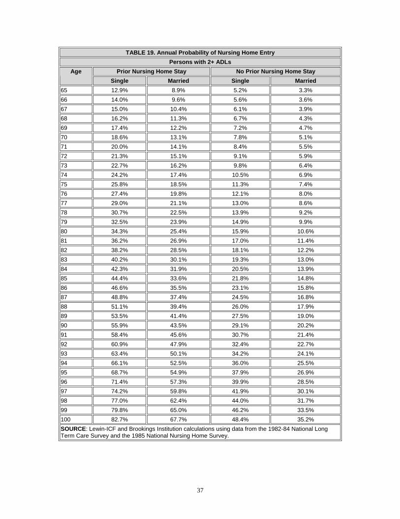
IV. LONG TERM CARE UTILIZATION ........................................................................ 35

A. Nursing Home Utilization .................................................................................... 35 B. Home Care Utilization......................................................................................... 46

V. LONG TERM CARE FINANCING ........................................................................... 56

A. Nursing Home Care Financing ........................................................................... 56 B. Financing of Home Care Services ...................................................................... 62

ATTACHMENTS

MEMO 1 (2/14/89): 1988 Social Security Trustee’s and Bureau of the Census Population Projections ............................................A-1 MEMO 2 (6/6/89): SIPP Data on Support for Adults Living in Nursing Homes..................................................................................A-4 MEMO 3 (7/14/89): Status Report on Analysis of SIPP Data on Assets of the Elderly ............................................................................A-7 MEMO 4 (7/14/89): Profile of the SIPP Elderly Who Responded in 1984 but not 1985 .......................................................................A-19 MEMO 5 (8/1/89): Update on Savings Rate of Elderly Families, 1984-1985..........................................................................A-21 MEMO 6 (10/18/89): Induced Demand................................................................A-26

i

MEMO 7 (10/19/89): Disability and Income.........................................................A-38 MEMO 8 (1/9/90): Income and Asset Distribution of Elderly Families .............A-49 MEMO 9 (1/10/90): Additional Information on the Income and Asset Distribution of Elderly Families...........................................A-53 MEMO 10 (1/12/90): Additional Information on the Income and Asset Distribution of Elderly Families...........................................A-56 MEMO 11 (7/18/90): Life Insurance Values Held by the Elderly..........................A-57 MEMO 12 (4/9/91): Table Specs for Distribution of Assets and Income............A-58 MEMO 13 (4/25/91): Living Arrangement and Disability......................................A-61 MEMO 14 (5/16/91): Medigap Analysis Results Using the 1984 SIPP/CES Match File and the 1989 CES ............................................A-63

ii

LIST OF FIGURES AND TABLES FIGURE 1: Brookings/ICF Long-Term Care Financing Model ........................................ 3 FIGURE 2: Flowchart for Utilization of Long Term Care Services................................. 36 FIGURE 3: Utilization of Formal Home Care by the Elderly .......................................... 48 TABLE 1: Labor Force Participation Rates ................................................................... 9 TABLE 2: Unemployment Assumptions...................................................................... 10 TABLE 3: Consumer Price Index Assumptions Used in Forecasts............................. 11 TABLE 4: Assumed Real Earnings Differentials ......................................................... 12 TABLE 5: Percent Distribution of Workers by Industry of Employment Assumed in PRISM for Selected Years...................................................................... 13 TABLE 6: Pension Coverage Asumptions .................................................................. 14 TABLE 7: Probabilities that Married Individuals Will Choose to Elect the Joint and Survivors Option, by Size of Pension Benefit ...................................... 19 TABLE 8: Savings Plan Participation Assumptions .................................................... 19 TABLE 9A: Proportion of DC LSDs that are Rolled Over to an IRA, Pre-TRA .............. 19 TABLE 9B: Proportion of DC LSDs that are Rolled Over to an IRA, Post-TRA............. 20 TABLE 10: IRA Adoption Assumptions for Non-Covered Workers, by Age and Family Earnings Level ................................................................................ 21 TABLE 11: IRA Adoption Probabilities for Covered Workers in 1982 by Family Income and Age of Worker......................................................................... 22 TABLE 12: Probabilities of Contributing to an IRA in a Given Year Once Selected to Adopt an IRA .......................................................................................... 22 TABLE 13: Distribution of Elderly Persons by Personal Income and Asset Levels, 1984 ........................................................................................................... 23 TABLE 14: Disability Prevalence Rates for the Noninstitutionalized............................. 28

iii

TABLE 15: Annual Disability Transition Probability Matrices for the Noninstitutionalized Elderly ........................................................................ 29 TABLE 16: Disability Prevalence Rates for Noninstitutionalized Disability Insurance

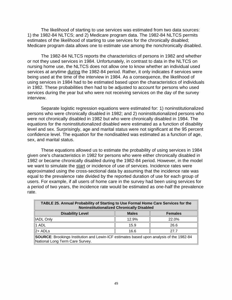
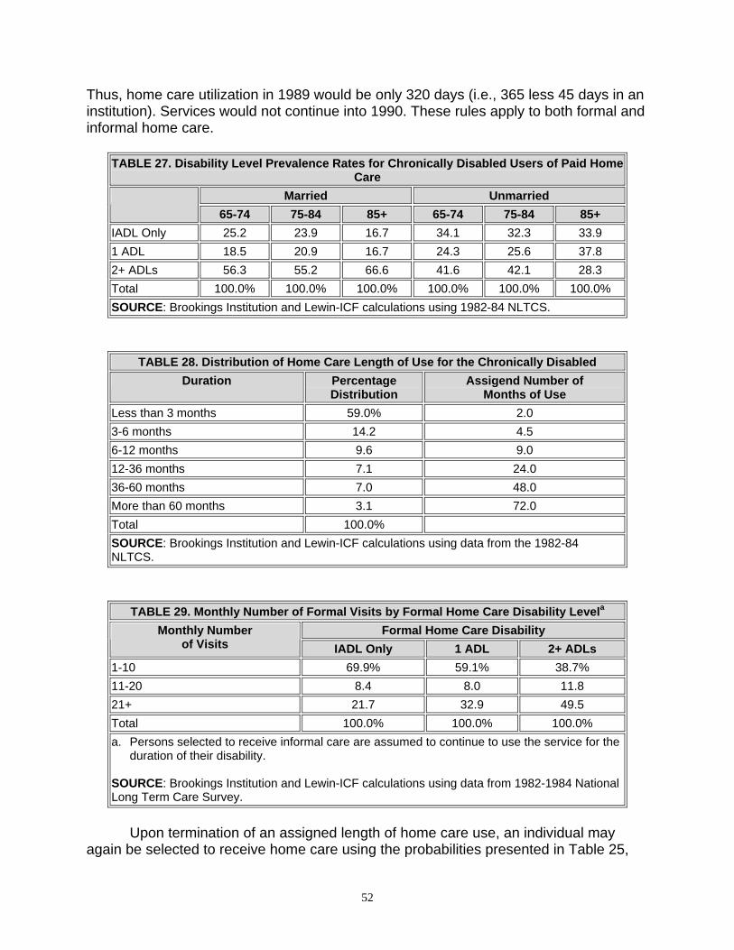
Recipients Simulated to Continue Begin Disabled at Age 65 ..................... 30 TABLE 17: Mortality Rates for the Noninstitutionalized Elderly in 1985........................ 31 TABLE 18: Mortality Adjustments Used in the Model ................................................... 34 TABLE 19: Annual Probability of Nursing Home Entry ................................................. 37 TABLE 20: The Probability of Nursing Home Length of Stay by Age of Entry and Marital Status.............................................................................................. 42 TABLE 21: Number of Nursing Home Days Assigned by Length of Stay Category...... 44 TABLE 22: Nursing Home Disability Prevalence Rates ................................................ 45 TABLE 23: Nursing Home Discharge Disability Prevalence Rates ............................... 46 TABLE 24: The Probability of Nursing Home Length of Stay by Age of Entry and Marital Status for Persons Using Services Due to Induced Demand.......... 47 TABLE 25: Annual Probability of Starting to Use Formal Home Care Services for the Noninstitutionalized Chronically Disabled............................................. 49 TABLE 26: Annual Probability of Starting to Use Formal Home Care for Persons Who are Noninstitutionalized and Nondisabled at the Start of the Year ..... 50 TABLE 27: Disability Level Prevalence Rates for Chronically Disabled Users of Paid Home Care ......................................................................................... 52 TABLE 28: Distribution of Home Care Length of Use for the Chronically Disabled ...... 52 TABLE 29: Monthly Number of Formal Visits by Formal Home Care Disability Level... 52 TABLE 30: Medicare Reimbursed Home Health Visits ................................................. 53 TABLE 31: Percentage of Noninstitutionalized Nonchronically Disabled Persons

Receiving Medicare Home Health Visits..................................................... 54 TABLE 32: Informal Home Care Prevalence Rates for the Chronically Disabled ......... 55 TABLE 33: Average Daily Rates for Nursing Home Care by Source of Payment ......... 56

iv

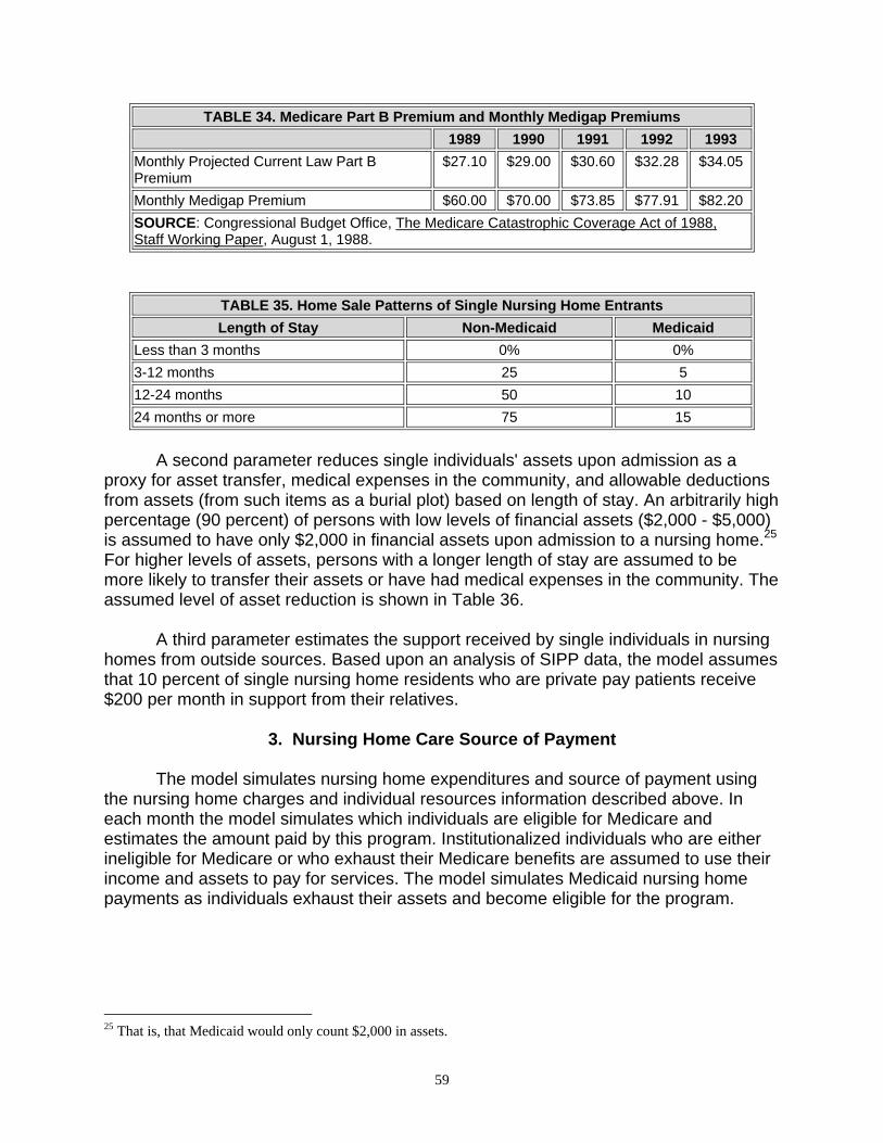
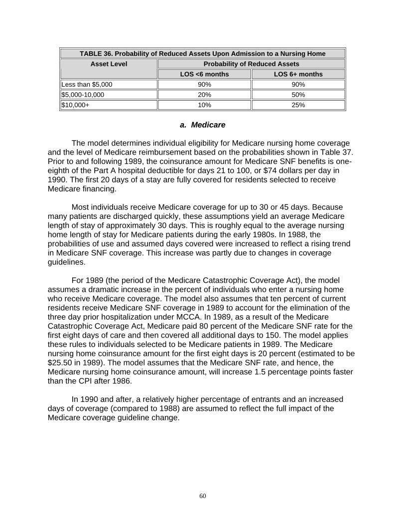
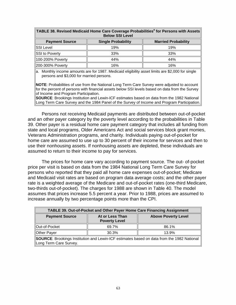
TABLE 34: Medicare Part B Premium and Monthly Medigap Premiums ...................... 59 TABLE 35: Home Sale Patterns of Single Nursing Home Entrants .............................. 59 TABLE 36: Probability of Reduced Assets Upon Admission to a Nursing Home.......... 60 TABLE 37: Likelihood of Receiving Medicare SNF Coverage and Length of Coverage.................................................................................................... 61 TABLE 38: Revised Medicaid Home Care Coverage Probabilities for Persons with

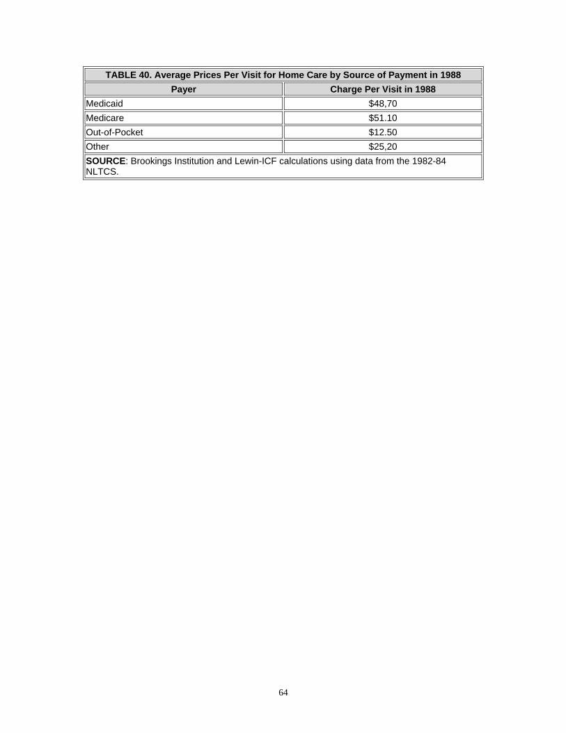
Assets Below SSI Level.............................................................................. 63 TABLE 39: Out-of-Pocket and Other Payer Home Care Financing Assignment........... 63 TABLE 40: Average Prices Per Visit for Home Care by Source of Payment in 1988.... 64

v

OVERVIEW OF THE PROJECT

In September of 1988, the Office of the Assistant Secretary for Planning and Evaluation (ASPE) contracted with Lewin-ICF and the Brookings Institution to develop a public use version of the Brookings/ICF Long Term Care Financing Model. Using microsimulation techniques, the model projects the utilization and sources of financing for nursing home and home care services among the elderly to the year 2020.

Under this contract, many of the assumptions used in the model were revised to reflect data and findings that had recently become available. As the need for alternative policy simulations arose, the capabilities of the model were expanded. Examples of the types of simulations modeled include: the purchase of new private long term care insurance products; the use of pension funds to purchase long term care insurance; and publicly sponsored programs, such as the long term care benefits proposed by the Pepper Commission.

One of the products of this project is a public use version of the model code and accompanying documentation. The documentation includes:

• Model Assumptions, which presents the assumptions used in developing the

model. • Designing and Using Model Simulations, which presents assumptions used in

modeling alternative proposals and using the results of the model.

• A User's Guide to Specifying Simulations, which details how to specify simulations using the model's parameters.

• A Programmer's/Operator's Manual, which shows the code structure and

operation of the model.

vi

PREFACE

This report is one of four related to the Brookings/ICF Long Term Care Financing Model. It outlines the assumptions used in developing the model. The three other documents discuss: 1) assumptions used in modeling alternative proposals and using the results of the model; 2) how to specify simulations using the model's parameters; and 3) the code structure and operation of the model.

This documentation was prepared by David L. Kennell and Lisa Maria B. Alecxih

of Lewin-ICF in collaboration with Joshua M. Wiener and Raymond J. Hanley of the Brookings Institution. John Drabek, serving as the project officer, and Paul Gayer of the Office of the Assistant Secretary for Planning and Evaluation provided invaluable comments.

This report was developed as part of the documentation of a public use version of the Brookings/ICF Long Term Care Financing Model for the Office of the Assistant Secretary for Planning and Evaluation. Other reports in this series include:

• Designing and Using Model Simulations • A User's Guide to Specifying Simulations • A Programmer’s/Operator’s Manual

Copies of the reports may be obtained by writing to:

Brenda Veazey Department of Health and Human Services Room 424E, Humphrey Building 200 Independence Avenue, S.W. Washington, D.C. 20201

vii

I. INTRODUCTION A. The Model’s Structure

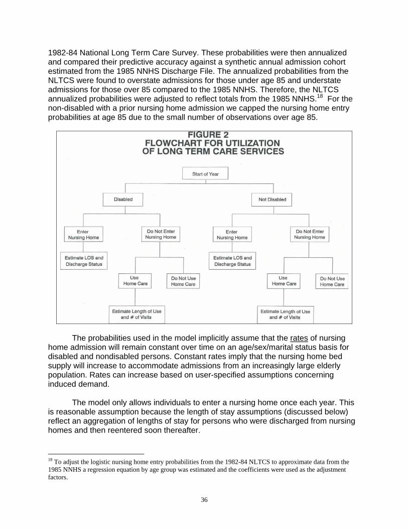
The Brookings/ICF Long Term Care Financing Model simulates the utilization and financing of long term care services -- both nursing home and home care -- for elderly individuals through 2020. Nursing home services include care provided by skilled nursing facilities (SNFs) and intermediate care facilities (ICFs). Home care services include home health, homemaker, personal care, and meal preparation services. The model simulates the number of individuals receiving these services and the costs of these services which are financed by various public and private sources. The overall objective of the model is to simulate the effects of various financing and organizational reform options on future public and private expenditures for nursing home and home care.

The two principal components of the model are the Pension and Retirement Income Simulation Model (PRISM) and the Long Term Care Financing Model. PRISM simulates future demographic characteristics, labor force participation, income and assets of the elderly. The Long Term Care Financing Model simulates disability, admission to and use of nursing home and home care, and methods of financing long term care services. The model uses national data and does not take into account regional, state or local variations.

The model begins with a nationally representative sample of the adult population with a record for each person's age, sex, income, and other characteristics. The model simulates changes for each individual's characteristics in the sample population from 1986 to 2020, including age, economic status, disability status, utilization of long term care, and the method of paying for such care.

The model uses a Monte Carlo simulation methodology. The model simulates changes in an individual's status by drawing a random number between zero and one and comparing it to the fixed probability of that event occurring for an individual with a given set of socio-demographic characteristics. For example, the annual probability of death for an 85 year old noninstitutionalized female is .03 (i.e., three out of every 100 women age 85 who are not in a nursing home are expected to die each year). If the random number drawn by the model is less than or equal to .03 for this 85 year old woman, then the individual is assumed to die in that year. If the number drawn lies between .03 and 1.0, then the individual is assumed to continue to live during that year. In order to reduce random variation due to the Monte Carlo procedure, the model is routinely run with two separate random number sets and the results are averaged.

The model can be used to simulate long term care financing assuming changes in private financing methods (such as increased purchase of private long term care insurance) or new public financing programs. These simulations are greatly affected by

1

the choice of assumptions about the economy (such as the rate of growth of the overall economy and nursing home prices) and individual behavior (such as rates of nursing home utilization, insurance purchases, and induced demand). The model can be used to make estimates using alternative assumptions to show how sensitive the results are to the assumptions chosen.

The current version of the model is a major revision of the model that was developed jointly by Lewin-ICF and the Brookings Institution in 1986. The model was revised in 1988 and 1989 using data from a number of newly available data sources, including the 1982-84 National Long Term Care Survey, the 1985 National Nursing Home Survey, the 1984 Survey of Income and Program Participation (Wave 4), and Medicaid and Medicare program data provided by the Health Care Financing Administration (HCFA).

The six major components of the model are described below. A flowchart of these components is shown in Figure 1.

Population Data Base: Using data from the May 1979 Current Population Survey, the model uses information for a nationally representative sample of 28,000 adult individuals of all ages in 1979. This 1979 data base was chosen because it has been merged with social security earnings histories for each individual in the sample.

Income Simulator: The Pension and Retirement Income Simulation Model (PRISM) simulates labor force activity, marital status, income, and assets for each individual. The probabilities in this part of the model are based upon Census Bureau data on the likelihood of marriage, work, etc. for different demographic groups. The economic assumptions underlying the simulations are generally those used in Alternative 11-13 of the 1988 Social Security Trustee's Report. The model estimates retirement income from private sector defined benefit pension plans, public pension plans, social security, private sector defined contribution plans, Individual Retirement Accounts and Keoghs. The model also simulates the assets of elderly individuals including the value of home equity.

Disability of the Elderly: Using probabilities estimated primarily from the 1982-84 National Long Term Care Survey (NLTCS) and the 1985 National Nursing Home Survey (NNHS), this part of the model simulates the level of disability for persons age 65 and over. The model simulates the onset of disability, the level of disability, changes in disability, and recovery from disability.

Utilization of Long Term Care Services: This part of the model uses probabilities estimated from the 1982-84 NLTCS and the 1985 NNHS to simulate admission to and length of stay in a nursing home. For noninstitutionalized persons, the model also simulates the use and length of stay for paid home care services using probabilities derived primarily from the 1982-84 NLTCS and Medicare program data.

2

FIGURE 1. Brookings/ICF Long Term Care Financing Model

Sources and Levels of Payment: The fifth component of the model simulates the sources of payment and the level of expenditures for each individual receiving nursing home or home care services. The model incorporates Medicare eligibility and coverage provisions and uses a set of uniform assumptions about the Medicaid

3

program, including provisions from the Medicare Catastrophic Coverage Act that were not repealed. State Medicaid program variations are not modeled.

Aggregate Expenditures and Utilization: The sixth part of the model accumulates Medicare, Medicaid, private expenditures, and utilization for each simulated individual for each year. The final output file from the model provides detailed information for individuals age 65 and older, for each year from 1986 to 2020, on individuals' age, sex, marital status, disability, sources and amounts of income, assets, and use of and payment sources for nursing home and home care services. This file is tabulated to show aggregate long term care expenditures for various demographic groups and sources of financing. B. Organization of the Documentation

This document describes both the retirement income simulation and the long term care financing portions of the model. The retirement income simulations are described in more detail separately (see David L. Kennell and John F. Shells, "The ICF Pension and Retirement Income Simulation Model (PRISM) with the Brookings/ICF Long Term Care Financing Model," September 1986). Section II of the documentation describes the key demographic and retirement income assumptions in the model. Section III describes the probabilities used in the model to simulate disability and mortality for the elderly. Section IV describes the simulation of utilization of nursing home and home care services. Section V describes the financing of nursing home and home care services. Memos on data analyses related to the model are included as attachments.

4

II. KEY DEMOGRAPHIC AND RETIREMENT INCOME ASSUMPTIONS

The Pension and Retirement Income Simulation Model (PRISM) develops future estimates of retirement income.1 The model simulates retirement incomes for a sample of individuals age 25 and older in 1979 obtained from the ICF Pension/Social Security Data Base. The sources of income modeled in PRISM include: social security, employer pensions, Individual Retirement Accounts and Keogh accounts, employment earnings, asset income, and Supplemental Security Income (SSI) program benefits. PRISM simulates retirement income for this sample of the individuals based upon: (1) the characteristics of individuals in 1979; (2) their family and work histories prior to 1979; and (3) simulations of the future workforce experience of these individuals.

In order to simulate the future workforce experience and retirement incomes of these individuals, the model requires a large number of assumptions concerning the likelihood of future events for each individual, such as the likelihood an individual will continue to work, whether he or she will become divorced or married, and whether he or she will contribute to an IRA. These assumptions are divided into eight major areas:

• demographic • labor force and economic; • pension coverage; • social security and the retirement decision; • employer pension provisions; • Individual Retirement Accounts; • housing and financial assets; and • Supplemental Security Income benefits.

The key assumptions used in each of these areas are summarized below. We

start by briefly summarizing the PRISM modeling system. A. PRISM Modeling System

The Pension and Retirement Income Simulation Model (PRISM) simulates the distribution of retirement income from both public and private resources for elderly families. PRISM models income from social security, private and public employee retirement plans, Individual Retirement Accounts (IRAs) and Keogh accounts, earnings, assets, and the Supplemental Security Income (SSI) program. It also estimates taxes paid in retirement. 1 For a more detailed discussion of the PRISM simulation methodology and assumptions see: David L. Kennell and John F. Sheils,"The ICF Pension and Retirement Income Simulation Model (PRISM) with the Brookings/ICF Long-Term Care Financing Model," ICF Incorporated, Washington, D.C., September 1986.

5

The model simulates the distribution of retirement income among households of

various socioeconomic groups for a representative sample of individuals age 25 and older in 1979 obtained from the ICF Pension/Social Security Database. These data are an exact match of the Special Pension Supplement to the May 1979 Current Population Survey (CPS) and Social Security Administration (SSA) earnings history data for 1951 through 1977.

For each individual in the population data base, PRISM uses probabilities estimated primarily from recent Census data to simulate each individual's earnings, periods of employment, and family structure between 1979 and the date of retirement. To ensure that PRISM simulations of labor force participation and earnings are consistent with the projected aggregate growth of the economy, we linked PRISM to the September 1987 labor force projections made by the Bureau of Labor Statistics.

Using the simulated work histories, the model calculates the social security benefits and IRA accumulations for each individual, as well as SSI benefits and earning from employment once the individual reaches retirement age, When individuals are simulated to enter a pension-covered job, the model assigns them to an actual pension plan sponsor selected from a representative sample of private and public retirement plan sponsors (the ICF Retirement Plan Provisions Data Base). When these individuals meet the plans' eligibility standards, PRISM then calculates their benefits using the plans' actual benefit provisions. This process of matching a representative sample of individuals to a representative sample of plan sponsors is a unique feature of PRISM. The model also estimates the amount of individuals' assets in retirement based upon the distribution of assets reported in the 1984 Panel of the Survey of Income and Program Participation (SIPP). Separate amounts are estimated for financial assets and home equity. Individuals are assumed to receive income from their nonhousing assets. B. Demographic Assumptions

PRISM simulates mortality, disability, child bearing, and changes in marital status. During each simulation year, individuals are simulated to die, become disabled, recover from disability, bear children, and become married or divorced. The model uses a variety of assumptions to estimate these events, most of which are consistent with the Alternative II-B assumptions used in the 1988 report of the Trustees of the Old Age and Survivors Insurance and Disability Insurance Trust Funds (“1988 Trustees' Report”). The major assumptions are discussed below.

• Mortality -- PRISM uses the Alternative II-B mortality assumptions used in the

1988 Trustees' Report. Mortality rates vary by age, sex, disability status, and years since becoming disabled. Mortality rates vary for each simulation year to reflect projected improvements in mortality made by the Social Security Actuaries. As discussed in a later section, mortality adjustments are made for

6

persons 65 and over to reflect differences in mortality between institutionalized and noninstitutionalized, disabled and nondisabled persons.

• Disability -- For persons under 65, PRISM uses the rates of disability used in the

1988 Trustees' Report. These rates vary by age and sex and are assumed to remain unchanged over time. Disability for persons age 65 and over is discussed in Section III.

• Recovery from Disability -- For persons under 65, PRISM uses rates of disability

recovery developed by the Social Security Actuaries for 1979-1980. These rates vary by age, sex, and years since becoming disabled. These are the most recent rates available and are assumed to remain unchanged over time. Recovery from disability for the elderly is discussed in Section III.

• Child Bearing -- Fertility rates in the model are based upon an analysis of Census

Bureau data on women who gave birth to children during the 1976-1980 period. These fertility rates vary by age, marital status, employment status, and number of children. In the model, these rates are constrained to match the Alternative II-B assumptions of fertility in the 1988 Trustees' Report.

• Marital Status -- All probabilities concerning marriage and divorce are obtained

from Monthly Vital Statistics data developed by the National Center for Health Statistics. The aggregate rates match the Alternative II-B projections in the 1988 Trustees' Report. Divorce rates vary by the age of husband and wife. Marriage rates vary by age, sex and marital status (i.e., never married, divorced, or widowed) of the individual. In the model, individuals selected to become married are joined with a member of the opposite sex based upon data on the distribution of newly married individuals by age and education of husband and wife reported in Vital Statistics data. The marriage and divorce rates are assumed to remain constant in the future.

C. Labor Force and Economic Assumptions

PRISM simulates each individual's employment history from 1979 (the date of the May 1979 CPS survey) through the date of retirement. During each simulation year, the model simulates wage rates, hours worked, job change and industry of employment. The simulations were constrained to match September 1987 Bureau of Labor Statistics (BLS) projections of employment and industry composition, and the Alternative II-B assumptions from the 1988 Trustees' Report of average wage rates in future years. The major assumptions are as follows:

• Employment Levels Over Time -- PRISM was constrained to simulate aggregate

levels of employment consistent with BLS forecasts of labor force participation

7

rates for 1987-2000 (see Table 1).2 Labor force participation rates after 2000 are assumed to remain constant for each age/sex group. These forecasts include: 1) trends in employment for men and women of various age groups; 2) projections of economic growth; and 3) trends in the age of retirement. Unemployment rates from the 1988 Trustees' Report for the years 1986-2020 were used (see Table 2). Actual participation rates and unemployment rates are used for 1979 through 1987.

• Employment by Socio-Economic Group -- Given the levels of labor force

participation for different age/sex groups, the model simulates the number of hours each individual will work during each simulation year based upon an analysis of Bureau of the Census data on employment patterns during the 1976-80 period. For each individual, the decision to work and the number of hours worked in a year varies by age, sex, hours worked in each of the three previous years, marital status, presence of children at various ages, pension receipt status, and social security benefit receipt status.

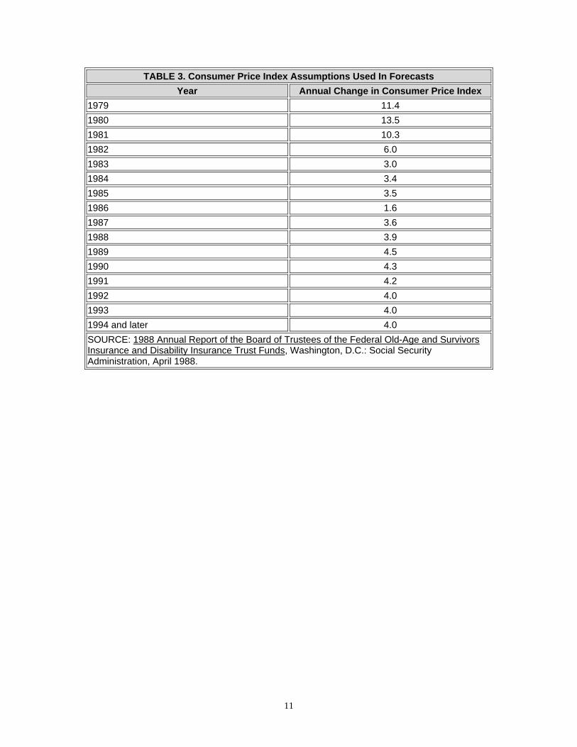
• Inflation -- Consumer prices are assumed to increase at the rate specified under

the Alternative II-B assumptions in the 1988 Trustees' Report. These price change assumptions are shown in Table 3.

• Interest Rates -- Assets in all defined contribution plans and individual retirement

accounts (IRAs) were assumed to earn interest at an average annual rate of 7.0 percent.

• Wage Growth -- Aggregate changes in wage levels are assumed to increase at

the rate assumed in the Alternative II-B assumptions of the 1988 Trustees' Report (see Table 4). In general, average wages are assumed to grow by 1.3-1.6 percentage points in excess of the inflation rate in each year after 1990. Actual wage growth rates are used during the 1979-87 period. Given these aggregate rates, the hourly wage rates for each individual in the model are adjusted during each year based upon an analysis of Census Bureau data on patterns of wage growth. Rates of wage growth vary by age, sex, and whether or not the individual changed jobs during the year.

• Job Change -- The probability that an individual will change jobs is based upon

an ICF analysis of Census Bureau data concerning job change patterns during 1979. Job change is modeled as a function of the age, part-time/full-time status and job tenure of each worker. These probabilities are assumed to remain constant over time.

• Maternity Job Terminations -- Women who have children often leave the labor

force. In some instances, these women may re-enter the labor force and resume

2 We were unable to use the 1988 Trustee's Report assumptions on labor force participation rates because they are not provided in a disaggregated fashion.

8

working for the same employers they had prior to having the child. In PRISM, we assume that a woman who has a child and leaves her job in the same year will become reemployed on the same job if: 1) the woman re-enters the labor force within five years of having the child; and 2) the woman became employed in the same industry she was in prior to having the child.

• Industry Changes -- PRISM assigns individuals to an industry of employment

when they change jobs or enter the labor force. The industry assigned to these individuals varies with age, full time/part time status, and industry of prior job. As shown in Table 5, the model assumes that over time, a higher proportion of workers work in the services industries and a lower proportion of workers work in the manufacturing industry. These industry composition estimates are based upon November 1987 BLS projections for the 1987-2000 period. After 2000, industry composition is assumed to remain constant.

TABLE 1a. Labor Force Participation Rates

1984 1985 1986 1987 1988 1989 1990 1991 1992 1993 1994 1995 1996 1997 1998 1999 2000and

After MEN 16-17 43.5 45.1 45.3 45.6 45.8 45.9 46.1 46.5 46.7 46.9 47.2 47.4 47.7 47.9 48.3 48.6 48.7 18-19 68.1 68.9 68.3 68.5 68.9 69.1 69.3 69.5 69.8 70.1 70.4 70.7 71.0 71.3 71.5 71.9 72.2 20-24 85.0 85.0 85.8 85.9 86.0 86.2 86.3 86.5 86.5 86.7 86.8 86.8 86.9 87.1 87.3 87.3 87.5 25-34 94.3 94.7 94.6 94.3 94.2 94.2 94.1 94.0 94.0 93.9 93.8 93.9 93.7 93.7 93.7 93.6 93.6 35-44 95.4 95.0 94.8 94.6 94.4 94.4 94.4 94.3 94.2 94.2 94.1 94.1 94.0 94.0 94.0 93.9 93.9 45-54 91.2 91.0 91.0 90.9 90.8 90.8 90.7 90.7 90.7 90.6 90.6 90.6 90.5 90.4 90.3 90.2 90.1 55-59 80.2 79.6 79.0 78.6 78.3 78.1 77.8 77.6 77.4 77.0 76.8 76.6 76.3 76.0 75.8 75.5 75.2 60-61 68.1 68.9 67.7 66.9 66.4 66.0 65.5 65.0 64.5 64.0 63.5 63.2 62.8 62.1 61.7 61.3 60.9 62-64 47.5 46.1 45.8 44.9 44.3 43.7 43.0 42.5 42.0 41.5 40.9 40.4 39.9 39.4 39.1 38.6 38.2 65-69 24.5 24.4 25.0 24.2 23.7 23.0 22.5 22.1 21.5 20.9 20.5 20.1 19.7 19.2 18.7 18.3 17.9 70-74 16.0 14.8 14.3 14.0 13.6 13.2 12.9 12.5 12.1 11.7 11.3 11.0 10.6 10.2 10.0 9.6 9.3 75+ 7.5 7.0 7.1 7.0 6.8 6.5 6.3 6.1 5.8 5.7 5.4 5.2 5.1 4.9 4.7 4.5 4.3 WOMEN 16-17 41.2 42.1 43.7 44.7 45.1 45.6 46.1 46.6 47.1 47.5 48.0 48.3 48.7 49.1 49.3 49.6 49.7 18-19 61.8 61.7 62.3 62.7 63.3 63.8 64.1 64.4 64.9 65.4 65.9 66.3 66.8 67.2 67.7 68.1 68.6 20-24 70.4 71.8 72.4 72.6 73.1 73.6 74.2 74.6 75.1 75.5 76.0 76.4 76.7 77.3 77.7 78.0 78.4 25-34 69.8 70.9 71.6 72.4 73.3 74.3 75.2 76.0 76.9 77.6 78.4 79.2 79.8 80.5 81.1 81.7 82.3 35-44 70.2 71.8 73.1 73.9 74.9 75.9 76.9 77.8 78.7 79.5 80.3 81.0 81.7 82.4 83.0 83.7 84.2 45-54 62.9 64.4 65.9 66.4 67.3 68.1 69.0 69.7 70.5 71.2 72.0 72.7 73.4 73.8 74.4 74.9 75.4 55-59 49.8 50.3 51.3 51.5 51.8 52.1 52.4 52.7 53.1 53.3 53.6 53.9 54.2 54.5 54.7 55.0 55.3 60-61 40.0 40.3 40.0 40.2 40.3 40.3 40.3 40.4 40.4 40.4 40.5 40.5 40.5 40.6 40.6 40.6 40.6 62-64 28.8 28.6 28.5 28.7 28.8 28.8 28.8 28.9 28.9 28.9 28.9 28.9 28.9 28.9 29.0 29.0 29.0 65-69 14.2 13.5 14.3 14.0 13.8 13.6 13.4 13.3 13.1 12.9 12.7 12.5 12.3 12.1 11.8 11.6 11.4 70-74 7.3 7.6 6.9 7.1 7.1 7.0 7.0 6.9 6.9 6.8 6.7 6.7 6.7 6.6 6.6 6.5 6.5 75+ 2.5 2.2 2.4 2.4 2.4 2.3 2.2 2.1 2.1 2.0 1.9 1.9 1.8 1.7 1.7 1.6 1.5 a. Participation rates are expressed as percentages. SOURCE: Howard N. Fullerton, Jr., "Labor Force Projections 1986-2000," Bureau of Labor Statistics' Monthly Labor Review, September 1987.

9

TABLE 2. Unemployment Assumptions

Year Average Annual Unemployment Rate 1979 5.8% 1980 7.1 1981 7.6 1982 9.7 1983 9.6 1984 7.5 1985 7.2 1986 7.0 1987 6.2 1988 6.0 1989 6.2 1990 6.1 1991 6.0 1992 5.9 1993 5.8 1994 5.8 1995 5.8 1996 5.8 1997-1999 5.7 2000 and later 6.0 SOURCE: Alternative II-B assumptions from the 1988 Annual Report of the Board of Trustees of the Federal Old Age and Survivors Insurance and Disability Insurance Trust Funds, April 1988.

10

TABLE 3. Consumer Price Index Assumptions Used In Forecasts Year Annual Change in Consumer Price Index

1979 11.4 1980 13.5 1981 10.3 1982 6.0 1983 3.0 1984 3.4 1985 3.5 1986 1.6 1987 3.6 1988 3.9 1989 4.5 1990 4.3 1991 4.2 1992 4.0 1993 4.0 1994 and later 4.0 SOURCE: 1988 Annual Report of the Board of Trustees of the Federal Old-Age and Survivors Insurance and Disability Insurance Trust Funds, Washington, D.C.: Social Security Administration, April 1988.

11

TABLE 4. Assumed Real Earnings Differentials Year Real Earnings Differentiala

1979 -2.2% 1980 -4.4 1981 -1.0 1982 0.6 1983 1.8 1984 2.3 1985 0.7 1986 2.8 1987 -0.6 1988 0.9 1989 1.1 1990 1.1 1991 1.3 1992 1.7 1993 1.6 1994 1.6 1995 1.5 1996 1.5 1997 1.5 1998 1.4 1999 1.4 2000 and later 1.4 a. The real earnings differential is the difference between wage growth and the change in the

CPI. SOURCE: Alternative II-B assumptions from the 1988 Annual Report of the Board of Trustees of the Federal Old Age and Survivors Insurance and Disability Insurance Trust Funds, April 1988.

12

TABLE 5. Percent Distribution of Workers by Industry of Employment Assumed in PRISM for Selected Years

Industry 1980 1982 1984 1990 2000 and After

Mining 0.59% 0.95% 1.30% 0.88% 0.78% Construction 4.53 4.20 4.44 4.81 4.62 Manufacturing 20.78 19.08 18.73 16.32 14.09 Transportation 5.02 5.03 5.32 4.96 4.74 Trade 18.71 19.24 19.26 19.86 20.58 Finance 5.09 5.32 5.38 6.09 6.06 Service 17.55 18.50 18.50 20.34 23.08 State & Local 12.96 12.96 12.61 12.29 11.73 Federal 3.28 3.28 3.26 3.07 2.79 Self Employed 9.55 9.85 9.63 10.06 10.45 Agriculture 1.64 1.65 1.55 1.29 1.07 Total 100.00% 100.00% 100.00% 100.00% 100.00% SOURCE: Lewin-ICF estimates based upon George T. Silverstri and John M. Lukasiewicz, "A Look at Occupational Employment Trends to the Year 2000," Bureau of Labor Statistics' Monthly Labor Review, September 1987.

D. Pension Coverage Assumptions

For each job individuals have during the simulation, PRISM determines whether they are covered by a retirement plan and assigns covered workers to actual pension plan sponsors in the ICF Retirement Plan Provisions Data Base. Coverage rates were assumed to remain constant through time. The key assumptions are presented below.

• Pension Coverage -- As workers change jobs or enter the labor force during the

simulation, retirement plan coverage is simulated using coverage rates reported for job changers and labor force entrants in the May 1979 CPS. The model is further constrained to replicate coverage rates reported in the May 1983 EBRI/HHS CPS pension supplement. These coverage rates vary by the individual's industry of employment, full time/part time worker status, age, and real wage rate. Plan coverage on an industry basis is assumed not to change between 1983 and 1988 when the new nondiscrimination rules introduced in the 1986 Tax Reform Act became effective. The coverage rates assumed for 1979, 1983, and 1989 are presented in Table 6.

• Impact of 1986 Tax Reform Act on Pension Coverage -- Internal Revenue

Service's (IRS) pension plan nondiscrimination rules that became effective in 1989 stipulate that, in general, no more than 30 percent of a plan sponsor's employees could be excluded. Previously, employers could legally exclude up to

13

44 percent of their employees from the plan.3 The impact of this provision is modeled by estimating the number of persons in each industry who were not participating in a pension plan even though: (1) their employers sponsor a pension plan; and (2) they appear to meet the most restrictive age and service criteria allowed under ERISA (i.e., age 25 with at least 1,000 hours worked over a period of one year). In the model, the coverage rates for each industry are increased starting in 1989 so that no more than 30 percent of these individuals are not participating in their employer's plan (see Table 6).

• Plan Assignment -- Individuals are assigned to plan sponsors in the ICF

Retirement Plan Provisions Data Base in proportion to the number of individuals actually covered by that plan sponsor. PRISM assigns individuals to plans of similar industry, firm size, social security coverage status, union coverage status, multi/single employer plan status, and hourly/salary worker status. In addition, individuals are assigned only to plans which are consistent with the characteristics of the plan the individual reported he was covered by in the May 1979 CPS. To do this, the model takes into account the individual's reported participation and vesting status as well as plan contribution requirements and participation in a supplemental plan.

TABLE 6. Pension Coverage Assumptions

Pension Coverage Rate Industry 1979 1983 1989

Federal Government .93 .93 .93 State & Local Government .88 .83 .83 Mining .82 .75 .79 Manufacturing .76 .70 .73 Transportation .75 .75 .77 Finance .67 .67 .75 Construction .43 .41 .43 Trade .43 .46 .51 Services .43 .47 .52 Agriculture .19 .22 .22 Self Employed .14 .14 .14 SOURCE: Coverage rates for 1979 were derived from an ICF analysis of the May 1979 Current Population Survey. Coverage rates for 1983 are based on an ICF analysis of the May 1983 EBRI/HHS CPS Pension Supplement. Coverage rates for 1989 were estimated by ICF by adjusting the 1983 coverage rates to reflect the potential impact of the nondiscrimination rules in the Tax Reform Act of 1986.

3 The Tax Reform Act required that plans satisfy at least one of the following requirements: (1) the plan benefits at least 70 percent of all non-highly compensated employees; (2) the plan benefits a percentage of non-highly compensated employees which is at least 70 percent of the percentage of highly compensated employees benefiting under the plan; or (3) the average benefit percentage for non-highly compensated employees is at least 70 percent of the average benefit percentage for highly compensated employees.

14

E. Social Security and the Retirement Decision

The model simulates the acceptance of early, normal and late retirement benefits from both pension plans and social security. Current social security legislation provisions (including the 1983 amendments which increased the age at which unreduced benefits will be available) were assumed to be in place throughout the simulation. The important assumptions in the retirement decision are summarized below.

• Social Security Benefit Acceptance -- PRISM simulates the age at which

individuals start to receive social security benefits. These benefit acceptance rates vary by the age and sex of the individual. The rates were derived from social security benefit receipt data by age and sex during 1980. PRISM also assumes that eligible individuals age 62 or over will automatically accept benefits if they are disabled or unemployed or receiving an employer pension. These assumptions lead to an increase in social security early retirement because the number of individuals receiving pensions will increase over time in the simulations.

• Social Security Survivors Benefits -- Individuals are simulated to accept social

security survivors benefits in the first year they are eligible.

• Employer Pension Benefit Acceptance -- PRISM determines when an individual is eligible to accept employer pension benefits and then simulates the decision to accept the benefit. Benefit acceptance rates were developed by ICF based upon an analysis of Census Bureau data on pension benefit recipients.

• Impact of Eliminating Age 70 Mandatory Retirement -- Prior to 1987, employers

could legally require workers to retire when they reached age 70. Legislation passed in 1986 made such regulations illegal for most employers. All plans in the ICF Retirement Plan Data Base were modified to eliminate mandatory retirement beginning in 1987. The BLS labor force participation projections take into account the expected impact of the elimination of mandatory retirement.

• Acceptance of Deferred Vested Benefits -- Individuals who are vested and leave

their job prior to their eligibility for early or normal retirement receive a deferred vested benefit. These benefits are assumed to go into pay status when the individual reaches the plan's normal retirement age.

F. Employer Pension Plan Assumptions

PRISM simulates the size of the benefit individuals will receive from each pension plan in which they earn a benefit during the simulation. PRISM uses the actual provisions of the plan to which the individual was assigned to determine each

15

individual's eligibility and benefit amount. In general, pension plan provisions are assumed to remain unchanged over time except in instances where plan rules must be changed to be in compliance with the Retirement Equity Act of 1984 (REA) and the Tax Reform Act of 1986. The following assumptions are used:

• Benefit Formulas -- The benefit formulas in defined benefit plans are indexed to

changes in wages for “flat” and “unit” benefit formulas. Defined contribution plan salary bend points are also indexed to wage growth. Final pay defined benefit and all other parts of defined contribution plan formulas are held constant. No changes in participation, vesting or other plan provisions are assumed except where required by REA or the Tax Reform Act of 1986.

• Impact of REA on Participation Rules -- REA mandated that starting in 1985, the

minimum age requirement for participation would be reduced from 25 to 21 and that service between the age of 19 and 22 would be considered for determining vesting. Starting in 1985, the provisions of any private plans which were not already in compliance with these provisions are modified.

• Impact of the Tax Reform Act of 1986 on Vesting -- The Tax Reform Act required

private sector single-employer plans to vest benefits at least as rapidly as under the following two schedules: (1) full vesting upon completion of five years of service, or (2) 20 percent vesting after the completion of three years of service and 20 percent more for each subsequent year.4 Starting in 1989, the provisions of any private single employer plans which were not already in compliance with these provisions are modified.

• Limits on Social Security Integration -- Private sector plans which integrate

benefits with social security are required to limit their integration formulas. Although previous IRS regulations placed restrictions on how plans may integrate benefits, some low-wage workers had their pension benefits severely reduced or completely eliminated through integration. The Tax Reform Act retained and simplified IRS regulations on integration. In addition, the Act establishes additional restrictions on integration that apply separately to three types of integrated plans: − For defined benefit excess/step-rate (plans which calculate pension benefits

at different rates on earnings above and below specified levels), the rate at which benefits are provided for pay up to the integration level of a plan (the compensation amount below which pension benefits are reduced) may not be less than 50 percent of the rate at which benefits are provided in excess of that level. In addition, the integration level may not be more than the social security wage and benefit base.

− For defined benefit offset plans (plans where pension benefits are reduced by a stated percentage of the person's social security benefit), the offset may not reduce a participant's benefits by more than 50 percent.

4 An individual is "vested" in his/her plan when he or she has earned a nonforfeitable right to receive plan benefits.

16

− For defined contribution plans (plans where the employer contributes a specified amount but does not guarantee a specified benefit), the provisions are similar except that they apply to the rate of employer contributions. In addition, for defined contribution plans, the rate for pay in excess of the integration level may not exceed the rate for up to that level by more than the OASDI tax rate.

• Cost of Living Adjustments for Pensions -- The model assumes that benefits for

private plan beneficiaries from defined benefit plans will be indexed at half of the rate of inflation up to a maximum of two percent per year. All early and normal retirement benefits from the Civil Service Retirement Plan are assumed to increase at the annual rates of inflation shown in Table 3. State and local government benefits are assumed to increase at the rate of inflation up to a maximum of four percent each year. These assumptions are based upon a prior ICF study which analyzed cost of living adjustments over a ten year period for a representative sample of pension plans. None of these plans are assumed to index deferred vested benefits.

• Post-Retirement Survivors Benefit Option -- Table 7 presents the assumptions

used to determine which married individuals choose to elect the post-retirement joint and survivors option. Because REA mandated that starting in 1985 spousal consent is required to waive survivors benefit coverage, the model assumes that the rate of joint and survivor election will increase after the act is implemented (see Table 7). Individuals who accept the post-retirement survivors option are assumed to receive a 50 percent joint and survivor's annuity. This annuity provides a surviving spouse with a benefit equal to half of that received by the deceased individual while living.

• Pre-retirement Survivors Option -- Many plans automatically provide individuals

with pre-retirement survivor's coverage. In these plans, all individuals are assumed to "elect" the pre-retirement survivors option. In the other defined benefit plans, the model assumes 60 percent of married individuals will elect the pre-retirement survivors option. Because REA mandated spousal consent for waiver of the survivors coverage, the model assumes that 85 percent of all married individuals elect this option after REA is implemented.

• Vested Beneficial Survivors Benefits -- As mandated by REA, pre- retirement

survivors coverage was extended to spouses of individuals who receive vested benefits. Thus, the model simulates survivors benefits for spouses of vested beneficiaries who die between the time they leave the job and the date the benefits would have gone into pay status. In all instances the survivors benefit is assumed to be a 50 percent joint and survivors annuity.

• Maternity -- Under REA, workers who leave a pension plan may return to the job

and retain their prior years of service for participation and vesting status provided the break in service was less than or equal to the greater of: (1) five years; or (2)

17

the number of years of service prior to the break. Although both men and women may benefit from this provision, it was intended to assist women who leave their job for maternity. Because reemployment by the same employer is modeled in maternity cases only, this rule is applied only to women in the model who have children. In addition, due to further REA liberalizations in crediting service for maternity cases, working women who have a child are assumed to receive one year of credited service for the year the child is born, regardless of the number of hours they worked.

• Participation in Savings, Thrift and 401(K) Plans -- Table 8 summarizes the

assumptions on participation in supplemental thrift, savings and 401(K) plans for those individuals who are eligible to participate in them. The participation rates are a function of a worker's wage level and the employer matching rate.

• Employee Contributions -- In plans which require employee contributions as a

condition for plan participation, the model assumes individuals contribute the amount required to obtain the maximum employer contribution.

• Lump Sum Payments -- In the current version of PRISM, individuals who are

vested in a defined contribution plan and change jobs are selected to roll their lump sum payment into an IRA on the basis of lump sum rollover data obtained from an analysis of the May 1983 EBRI/HHS CPS Pension Supplement.5 The likelihood of a rollover varies by age, marital status, benefit level, and income. Among individuals age 55 or older, all lump sums over $1,750 are rolled over into an IRA and saved for retirement.

• Impact of Tax Reform Act on Roll-Overs -- The Tax Reform Act eliminated 10

year averaging, thus increasing individuals' incentives to roll-over into an IRA lump sum distributions received from a pension plan. Individuals age 59½ or older are permitted to make a one-time election to use 5-year forward averaging for a lump sum distribution which is not rolled-over into an IRA. Also, individuals attaining age 50 prior to January 1, 1986, may also make a one time election to use 5 year averaging for a lump sum distribution. The proportion of individuals who roll-over lump-sum distributions and save these assets for retirements was increased by 20 percent to model the impact of these provisions. These assumptions are shown in Table 9A and Table 9B.

• Lump Sum Payments at Retirement Income -- Individuals are assumed to draw

upon their defined contribution lump sum payments (those which were not cashed out) in the form of an annuity. This annuity is assumed to start at the earlier of: (1) the age they accepted social security benefits or (2) the year they first started receiving a defined benefit pension, but not earlier than age 55.

5 This analysis was conducted by Larry Atkins. Current law permits individuals to "roll over" any lump sum pension payment into an IRA in order to defer payment of taxes on this income until these benefits are drawn upon as income after reaching age 59½.

18

TABLE 7. Probabilities That Married Individuals Will Choose to Elect the Joint and Survivors Option, by Size of Pension Benefit

Probability of Choosing the Post-Retirement Joint and Survivor's Option

Pension Benfit Size (in 1980 dollars)

Before REA After REA Less than $3,000 25% 75% $3,000 or over 65% 80% SOURCE: Lewin-ICF assumptions.

TABLE 8. Savings Plan Participation Assumptions Employer Match RatebHourly Wage Levela

Low Medium High Less than $4 20% 25% 30% $4-$7 40% 50% 60% More than $7 60% 75% 90% a. Earnings level in 1980 dollars. b. Plans that match one dollar of employees contributions with less than fifty cents of employer

contributions are low match plans. Plans that match one dollar of employee contributions with fifty to ninety-nine cents are medium match plans. Plans that match one dollar of employee contributions with one dollar or more of employer contributions are high match plans.

SOURCE: Lewin-ICF assumptions.

TABLE 9A. Proportion of DC LSDs That Are Rolled Over to an IRA, Pre-TRA Under Age 30 Age 30-34 Age 45-54 Age 55-61 Age 62 or more Earnings

(1983 $s) <$3,500 $3,500+ <$3,500 $3,500+ <$3,500 $3,500+ <$3,500 $3,500+ <$3,500 $3,500+ NOT COLLEGE GRADUATE <$20,000 0.019 0.000 0.013 0.050 0.028 0.143 0.000 1.000 1.000 1.000 $20,000+ 0.024 0.000 0.041 0.091 0.105 0.211 0.000 1.000 1.000 1.000 COLLEGE GRADUATE <$20,000 0.037 0.000 0.015 0.061 0.075 0.364 0.000 1.000 1.000 1.000 $20,000+ 0.040 0.154 0.051 0.178 0.120 0.450 0.000 1.000 1.000 1.000

19

TABLE 9B. Proportion of DC LSDs That Are Rolled Over to an IRA, Post-TRA Under Age 30 Age 30-34 Age 45-54 Age 55-61 Age 62 or more Earnings

(1983 $s) <$3,500 $3,500+ <$3,500 $3,500+ <$3,500 $3,500+ <$3,500 $3,500+ <$3,500 $3,500+ NOT COLLEGE GRADUATE <$20,000 0.023 0.000 0.016 0.060 0.034 0.172 0.000 1.000 1.000 1.000 $20,000+ 0.029 0.000 0.049 0.109 0.126 0.253 0.000 1.000 1.000 1.000 COLLEGE GRADUATE <$20,000 0.044 0.000 0.018 0.073 0.090 0.437 0.000 1.000 1.000 1.000 $20,000+ 0.048 0.185 0.061 0.214 0.144 0.054 0.000 1.000 1.000 1.000

G. Individual Retirement Account Assumptions

PRISM models the accumulation of IRA savings. The assumptions used in this analysis are derived primarily from IRA participation data provided in the May 1983 EBRI/HHS CPS pension supplement. ICF recalibrated the assumptions used in these simulations so that PRISM assumptions are consistent with the 1983 estimates of: (1) the number of individuals participating in IRAs; and (2) the amount of IRA assets accumulated. The key assumptions in our IRA simulations are summarized below. In addition, we modified the IRA subroutine of PRISM to reflect the impact of the 1986 Tax Reform Act on IRA savings.

• IRA Adoption for Non-Covered Workers -- Table 10 summarizes the assumptions

used in modeling the adoption of IRAs by non-pension covered workers. These estimates do not include workers assumed to roll over vested benefits into IRA arrangements. ICF estimated these adoption rates using May 1983 EBRI/HHS CPS pension supplement data on non-covered individuals establishing an IRA during 1982.

• IRAs for Covered Workers -- A separate set of IRA adoption probabilities were

developed for individuals covered by a pension plan which apply only to 1982 (shown in Table 11). These probabilities were estimated using the May 1983 EBRI/HHS CPS pension supplement data on covered workers who established an IRA in 1982. In years after 1982, the IRA adoption rates for covered workers are assumed to be the same as for non-covered individuals (see Table 9), except as described below.

• IRA Contributions -- Once an individual is selected to adopt an IRA, PRISM

simulates his or her decision to contribute to the account for each year after the IRA is established. The model assumes that individuals contribute only if they are employed during the year. All individuals are assumed to contribute in the year the IRA is established. In succeeding years, individuals are randomly selected to contribute to their account based upon the probabilities presented in Table 12. These probabilities were estimated using May 1983 EBRI/HHS CPS pension supplement data on the number of individuals with IRA accounts who are currently contributing.

20

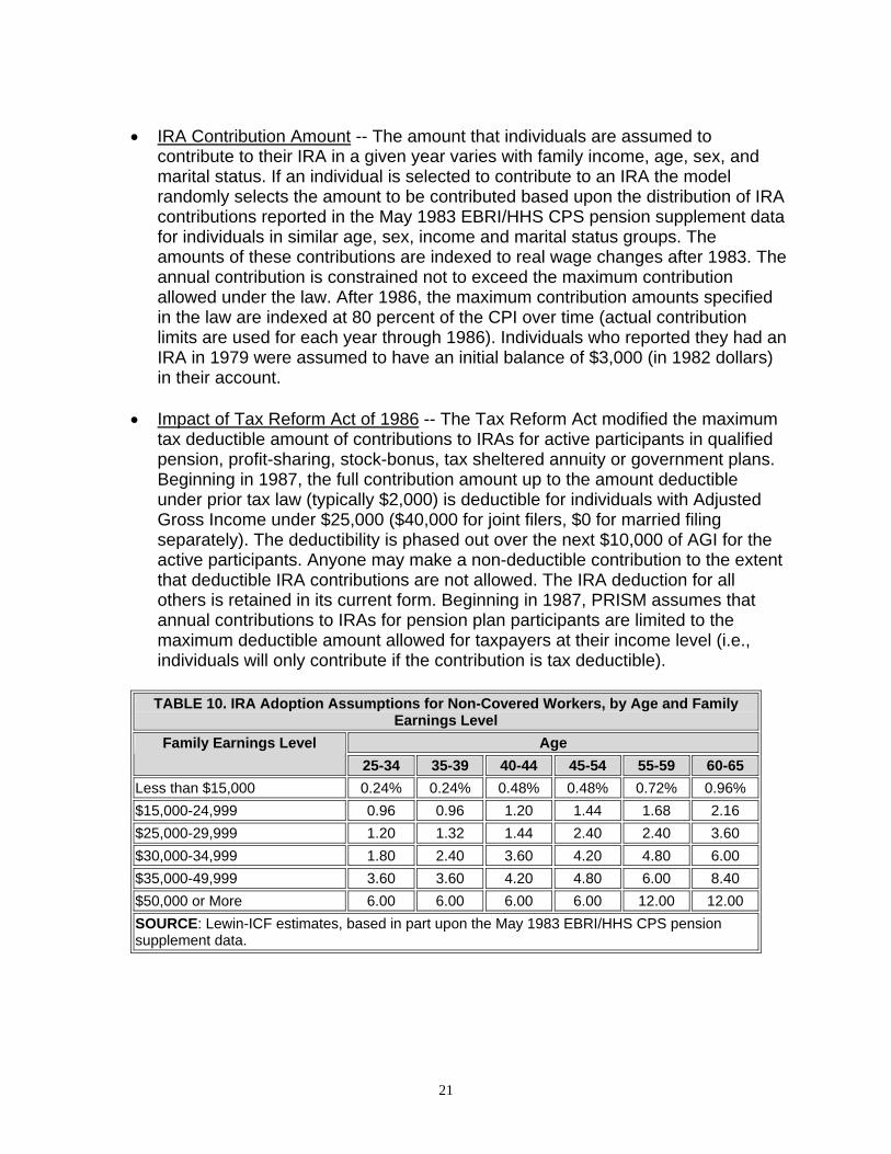
• IRA Contribution Amount -- The amount that individuals are assumed to

contribute to their IRA in a given year varies with family income, age, sex, and marital status. If an individual is selected to contribute to an IRA the model randomly selects the amount to be contributed based upon the distribution of IRA contributions reported in the May 1983 EBRI/HHS CPS pension supplement data for individuals in similar age, sex, income and marital status groups. The amounts of these contributions are indexed to real wage changes after 1983. The annual contribution is constrained not to exceed the maximum contribution allowed under the law. After 1986, the maximum contribution amounts specified in the law are indexed at 80 percent of the CPI over time (actual contribution limits are used for each year through 1986). Individuals who reported they had an IRA in 1979 were assumed to have an initial balance of $3,000 (in 1982 dollars) in their account.

• Impact of Tax Reform Act of 1986 -- The Tax Reform Act modified the maximum

tax deductible amount of contributions to IRAs for active participants in qualified pension, profit-sharing, stock-bonus, tax sheltered annuity or government plans. Beginning in 1987, the full contribution amount up to the amount deductible under prior tax law (typically $2,000) is deductible for individuals with Adjusted Gross Income under $25,000 ($40,000 for joint filers, $0 for married filing separately). The deductibility is phased out over the next $10,000 of AGI for the active participants. Anyone may make a non-deductible contribution to the extent that deductible IRA contributions are not allowed. The IRA deduction for all others is retained in its current form. Beginning in 1987, PRISM assumes that annual contributions to IRAs for pension plan participants are limited to the maximum deductible amount allowed for taxpayers at their income level (i.e., individuals will only contribute if the contribution is tax deductible).

TABLE 10. IRA Adoption Assumptions for Non-Covered Workers, by Age and Family

Earnings Level Age Family Earnings Level

25-34 35-39 40-44 45-54 55-59 60-65 Less than $15,000 0.24% 0.24% 0.48% 0.48% 0.72% 0.96% $15,000-24,999 0.96 0.96 1.20 1.44 1.68 2.16 $25,000-29,999 1.20 1.32 1.44 2.40 2.40 3.60 $30,000-34,999 1.80 2.40 3.60 4.20 4.80 6.00 $35,000-49,999 3.60 3.60 4.20 4.80 6.00 8.40 $50,000 or More 6.00 6.00 6.00 6.00 12.00 12.00 SOURCE: Lewin-ICF estimates, based in part upon the May 1983 EBRI/HHS CPS pension supplement data.

21

TABLE 11. IRA Adoption Probabilities for Covered Workers in 1982 by Family Income and Age of Worker

Age Family Earnings Level 25-34 35-39 40-44 45-54 55-59 60-65

Less than $15,000 4.0% 7.0% 4.0% 9.0% 13.0% 20.0% $15,000-24,999 8.0 8.0 9.0 17.0 27.0 19.0 $25,000-29,999 9.0 14.0 16.0 23.0 30.0 47.0 $30,000-34,999 16.0 20.0 19.0 28.0 46.0 51.0 $35,000-49,999 16.0 27.0 31.0 43.0 46.0 45.0 $50,000 or More 35.0 43.0 48.0 57.0 70.0 63.0 SOURCE: Lewin-ICF estimates, based in part upon the May 1983 EBRI/HHS CPS pension supplement data.

TABLE 12. Probabilities of Contributing to an IRA in a Given Year Once Selected to Adopt an IRA

Pension Coverage Status Family Earnings Level (in $ 1982) Covered Not Covered

Less than $25,000 48.0% 60.0% $25,000 or more 84.0 90.0 SOURCE: Lewin-ICF estimates, based in part upon the May 1983 EBRI/HHS CPS pension supplement.

H. Assets in Retirement

For many individuals, assets are an important factor in financing long term care expenditures. Annual income from assets may be used to purchase needed services. In many instances, individuals also liquidate assets to obtain the funds required to pay for care. Consequently, we developed a procedure for estimating asset levels and asset income in retirement for individuals. Both housing and non- housing (financial) assets are simulated.

The model simulates the level of assets and the income from thes e assets for persons age 65 and over in four steps. The model (1) assigns assets to persons age 65 and over in 1979; (2) assigns assets to persons who reach age 65 after 1979; (3) adjusts assets during retirement; and (4) simulates income from assets.

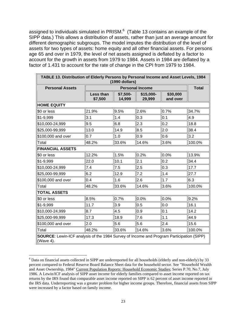
Asset Assignment in 1979 -- First, in 1979, each family unit age 65 and over is assigned a level of assets. This level of assets is based upon a distribution of assets from an analysis of the 1984 Survey of Income and Program Participation (SIPP) Wave 4. The model assigns individuals in PRISM the level of assets of similar individuals from the 1984 SIPP on the basis of age, marital status, income level and pension status. Actual records from the 1984 SIPP, adjusted for inflation and underreporting, are

22

assigned to individuals simulated in PRISM.6 (Table 13 contains an example of the SIPP data.) This allows a distribution of assets, rather than just an average amount for different demographic subgroups. The model imputes the distribution of the level of assets for two types of assets: home equity and all other financial assets. For persons age 65 and over in 1979, the level of net assets assigned is deflated by a factor to account for the growth in assets from 1979 to 1984. Assets in 1984 are deflated by a factor of 1.431 to account for the rate of change in the CPI from 1979 to 1984.

TABLE 13. Distribution of Elderly Persons by Personal Income and Asset Levels, 1984

(1990 dollars) Personal Income Personal Assets

Less than $7,500

$7,500- 14,999

$15,000- 29,999

$30,000 and over

Total

HOME EQUITY $0 or less 21.9% 9.5% 2.6% 0.7% 34.7% $1-9,999 3.1 1.4 0.3 0.1 4.9 $10,000-24,999 9.5 6.8 2.3 0.2 18.8 $25,000-99,999 13.0 14.9 8.5 2.0 38.4 $100,000 and over 0.7 1.0 0.9 0.6 3.2 Total 48.2% 33.6% 14.6% 3.6% 100.0% FINANCIAL ASSETS $0 or less 12.2% 1.5% 0.2% 0.0% 13.9% $1-9,999 22.0 10.1 2.1 0.2 34.4 $10,000-24,999 7.4 7.5 2.5 0.3 17.7 $25,000-99,999 6.2 12.9 7.2 1.4 27.7 $100,000 and over 0.4 1.6 2.6 1.7 6.3 Total 48.2% 33.6% 14.6% 3.6% 100.0% TOTAL ASSETS $0 or less 8.5% 0.7% 0.0% 0.0% 9.2% $1-9,999 11.7 3.9 0.5 0.0 16.1 $10,000-24,999 8.7 4.5 0.9 0.1 14.2 $25,000-99,999 17.3 18.9 7.6 1.1 44.9 $100,000 and over 2.0 5.6 5.6 2.4 15.6 Total 48.2% 33.6% 14.6% 3.6% 100.0% SOURCE: Lewin-ICF analysis of the 1984 Survey of Income and Program Participation (SIPP) (Wave 4).

6 Data on financial assets collected in SIPP are underreported for all households (elderly and non-elderly) by 33 percent compared to Federal Reserve Board Balance Sheet data for the household sector. See "Household Wealth and Asset Ownership, 1984" Current Population Reports: Household Economic Studies; Series P.70, No.7, July 1986. A Lewin/ICF analysis of SIPP asset income for elderly families compared to asset income reported on tax returns by the IRS found that comparable asset income reported on SIPP is 62 percent of asset income reported in the IRS data. Underreporting was a greater problem for higher income groups. Therefore, financial assets from SIPP were increased by a factor based on family income.

23

Asset Assignment After 1979 -- A similar procedure assigns a level and distribution of assets to individuals who reach the age of 65 after 1979. These probabilities are based upon the distribution and level of assets of persons who were age 65-67 in 1984 in SIPP. Before 1984, assets are reduced by a factor equal to the actual rate of change in the CPI over the time period. The level of assets from 1984 to the present is increased by the actual rate of change in the CPI, and then by the projected rate of change in the CPI assumed under the Alternative II-B assumptions.

Saving and Dissaving During Retirement -- Once assigned a level of assets, the assets of elderly families are adjusted over time to reflect that some elderly save and some dissave during retirement and that real estate generally appreciates. The value of net housing assets is assumed to increase 1.0 percentage points faster than the CPI. Based on an analysis of SIPP data over time, elderly families are assumed to save/dissave as follows:

• 35 percent save at a real rate of two percent annually (financial assets increase

two percentage points higher than the rate of change in the CPI); • 25 percent neither save nor dissave in real terms (financial assets increase at the

rate of change in the CPI); • 40 percent dissave at a real rate of two percent annual (financial asset levels

increase two percentage points less than the rate of change in the CPI). Some individuals who use long term care services will use their assets to pay for these services. This will accelerate this assumed rate of decrease. If an individual dies, his or her spouse receives all assets.7

Income from Assets -- Finally, the model calculates an assumed level of income from non-housing assets for family units age 65 and over. The model assumes that income from non-housing assets is 7 percent prior to 1989, 6.5 percent from 1989 to 1994, and 6 percent in 1995 and after. I. Supplemental Security Income Program Benefits

PRISM simulates the benefits from the Supplemental Security Income (SSI) program in three steps. The model (1) determines which families and individuals are eligible for SSI benefits using the SSI assets test, (2) estimates the annual benefit they would be entitled to receive from both the federal and state SSI programs, and (3) estimates which eligible families and individuals participate in the program. The SSI program is simulated in PRISM as described below.

7 Because we do not have data on the expected death benefits of life insurance policies, we assume that the spouses of deceased persons do not receive life insurance benefits. This should not have much effect on the asset holdings of widows because elderly persons tend not to have life insurance policies (60 percent have life insurance) and most of those with life insurance (80 percent) have a face value less than $10,000.

24

Program Filing Unit -- To determine the size of program benefits, elderly individuals are first formed into program "filing units." Each single individual forms one filing unit. Both members of a married couple are treated as a single filing unit, even if one member of the couple is ineligible (i.e., less than age 65). An individual under age 65 is assumed to be potentially eligible for SSI benefits for disabled persons if they are simulated to be disabled under the SSA definition of disability.

Asset Eligibility -- From 1979-83, to be eligible for SSI, individuals must have countable assets no greater than $1,500 for single individuals and $2,250 for married couples. This includes stocks, bonds, countable assets, cash, personal effects in excess of $1,500 and other non-housing assets. Home equity is not included in countable assets. As mandated by the Deficit Reduction Act of 1984 (DEFRA), beginning in 1984, the asset limit for single individuals increases by $100 and the limit for married couples increases by $150 each year until 1989, when they are equal to $2,000 and $3,000, respectively. After 1989, the asset limits are assumed to increase at 50 percent of the rate of increase in the CPI. The model determines asset eligibility by comparing the SSI program filing unit's financial assets, estimated as discussed in the prior section, to the appropriate asset limit.

Benefit Computation -- PRISM calculates net countable income for SSI filing units by summing eligible individuals' monthly countable incomes and subtracting allowable deductions. Countable incomes include eligible individuals' cash income from earnings, social security, pensions, assets, and income of an ineligible spouse. Allowable deductions include: (1) $20 of unearned income; (2) the first $65 of earnings plus 50 percent of earnings above $65; and (3) earnings income of an ineligible spouse up to one-half the maximum monthly federal benefit for a couple. The benefit amount is equal to the positive difference between the maximum monthly benefit and this monthly net income value. The maximum benefit levels vary by marital status, living situation, the presence of an ineligible spouse, and state of residence (see below).8

State Supplementation -- Forty-one states also provide some form of supplementary SSI benefit to elderly families. However, only 26 of these states provide a supplement to most or all of those who participate in the Federal SSI program while the remaining 15 states that supplement benefits do so for only a limited number of elderly facing unusual hardships (e.g., extraordinary expenses such as fire or moving related costs). PRISM estimates supplemental benefits only for the 26 states which provide supplements to most or all eligible individuals. Supplemental payments in these 26 states account for about 90 percent of all state supplemental benefits. These 26 state programs, all of which are administered by the federal government, use the same benefit formula as the one described above, with the exception that the maximum benefit is higher in these states. We assume that the state supplement amounts are fully indexed to inflation by the CPI.

8 Each individual's state of residence is assumed to remain the same as reported in the May 1979 CPS throughout the simulation.

25

Participation -- Not all eligible individuals chose to participate in the SSI program. Thus, only a portion of those simulated to be eligible for SSI are selected to receive these benefits. The SSI participation rates used in PRISM were estimated so as to replicate administrative data on the number of aged SSI recipients by marital status, family income level, and size of potential benefit.

26

III. DISABILITY AND MORTALITY OF THE ELDERLY

As discussed in the previous section, disability and mortality are modeled in different ways for persons under age 65 and persons age 65 and over. This section of the documentation describes the modeling of disability and mortality for persons age 65 and over. A. Disability

In the Brookings/ICF simulations, disabled individuals age 65 and over are defined as those who are unable to conduct at least one instrumental activity of daily living (doing heavy work, doing light work, preparing meals, shopping for groceries or other personal items, getting around inside, walking outside, managing money, and using the telephone) or unable to conduct at least any one of five activities of daily living (eating, bathing, dressing, toileting, and getting in and out of bed).9 In the model, when an individual turns 65 he or she will be assigned one of four disability levels: 1) a deficiency in one or more instrumental activities of daily living (IADL only); 2) a deficiency in one activity of daily living (1 ADL); 3) a deficiency in two or more activities of daily living (2+ ADLs); or 4) no disability.

The model measures the disability status of each individual at the start of each simulation year. During the year, a number of events occur which affect the number of disabled elderly persons:

− some persons become disabled; − some disabled persons become more disabled; − some disabled persons die; − some disabled persons become less disabled or recover from their disability;

and − some disabled persons age 64 turn age 65.

The model only notes intra-year changes for persons who start to use nursing home or home care services and for persons who are discharged from nursing homes. All other changes in disability status are assumed to occur at the start of the next simulation year. The model simulates each of these events using the probabilities described below.

As discussed above, during the year, the model simulates changes in an individual's disability status at the time of admission to or discharge from a nursing 9 In the 1982-1984 NLTC Survey, disability was defined as the inability to conduct any of the Activities of Daily Living or Instrumental Activities of Daily Living due to a health condition which had or would endure for 90 days or more.

27

home or starting to use noninstitutional services.10 At the start of each simulation year, the model also simulates transitions between disability levels for noninstitutionalized elderly persons, estimated from the 1982-1984 NLTCS (see Table 14). The model uses these transitions, but then controls to overall disability rater by simulating additional persons to become disabled each year to adjust for deaths or remissions from disability. In each simulation year, the model selects a sufficient number of individuals to become disabled so that the proportion of persons who are disabled in the community matches the disability prevalence rates shown in Table 14. These rates vary by level of disability, age, and marital status, and are assumed to hold constant over time.

The disability prevalence rates shown in Table 14 were calculated using data from the 1982-84 National Long Term Care Survey (NLTCS). The numerator of the disability prevalence rate in each age/disability level/marital status cell is equal to the number of disabled persons in that cell from the 1984 NLTCS. The denominator of the disability prevalence rate in each cell is equal to the total (disabled and non-disabled) number of persons in that cell from the 1984 NLTCS.

The transitions of non-institutionalized individuals from one disability level to another were estimated with data from the 1982-84 NLTCS. A set of transition matrices which estimate the probability that a person will be in one of the disability groups in 1984 based upon his or her disability status in 1982 were developed. Separate matrices for each of six age and marital status groups were estimated and the probabilities were then annualized.11 The annual disability transition probabilities for persons age 65 and over are shown in Table 15.

TABLE 14. Disability Prevalence Rates for the Noninstitutionalizeda

IADL Only 1 ADL 2+ ADLs Married Unmarried Married Unmarried Married Unmarried

65-69 3.79% 4.96% 1.74% 2.69% 3.45% 3.67% 70-74 5.01 6.62 2.68 3.73 5.11 4.66 75-79 6.90 8.64 3.24 5.77 7.71 7.15 80-84 10.34 11.25 6.03 8.07 12.93 11.35 85-89 11.36 13.64 7.57 11.21 21.77 15.81 90+ 7.50 15.45 20.00 13.69 26.25 31.35 a. Prevalence rates are expressed as percentages. SOURCE: Brookings Institution and Lewin-ICF calculations using data from the 1982-84 National Long Term Care Survey.

10 These disability transitions are described in the sections on nursing home and home care utilization. 11 A system of equations was estimated to compute the one-year probabilities.

28

TABLE 15. Annual Disability Transition Probability Matrices for the Noninstitutionalized Elderly Unmarried

Disability Level T2 Married

Disability Level T2 Disability Level T1

Non- Disabled

IADLOnly

1 ADL 2+ ADLs Non- Disabled

IADLOnly

1 ADL 2+ ADLs

AGE 65-74 Non-Disabled 95.80% 2.26% 1.02% 0.92% 97.00% 1.46% 0.59% 0.95% IADL Only 9.58% 71.90% 12.20% 6.32% 11.86% 70.10% 9.79% 8.25% 1 ADL 4.27% 25.15% 49.70% 20.88% 7.01% 18.55% 56.30% 18.14% 2+ ADLs 2.48% 8.87% 13.84% 74.80% 2.52% 7.36% 10.31% 79.80% AGE 75-84 Non-Disabled 90.80% 4.71% 2.67% 1.82% 93.50% 3.57% 1.08% 1.85% IADL Only 5.91% 66.10% 16.16% 11.83% 7.16% 71.00% 8.87% 12.96% 1 ADL 3.13% 19.10% 59.60% 18.16% 4.36% 19.20% 48.50% 27.93% 2+ ADLs 0.53% 6.88% 8.99% 83.60% 2.41% 6.84% 10.05% 80.70% AGE 85+ Non-Disabled 25.30% 28.51% 24.50% 21.69% 82.60% 7.51% 3.75% 6.14% IADL Only 0.45% 69.10% 15.23% 15.23% 2.37% 69.20% 11.85% 16.58% 1 ADL 0.62% 11.13% 56.70% 31.55% 3.96% 7.92% 48.50% 39.62% 2+ ADLs 0.46% 2.77% 7.37% 89.40% 0.00% 6.40% 8.00% 85.60% SOURCE: Lewin-ICF and Brookings calculations using the 1982-84 National Long Term Care Survey.

In the model, 60 percent of individuals receiving Disability Insurance (DI)

program benefits at age 62 are assumed to be "disabled" upon reaching age 65 (using the above definition of disability for persons 65 and over).12 "Disabled" individuals under age 65 are defined to be persons who meet the Social Security Administration's work disability eligibility criteria for Disability Insurance program benefits. Although this definition of disability is appropriate for simulating the receipt of Disability Insurance benefits for persons under 65, it is an inappropriate definition to use in simulating disability for the elderly for the use of long term care services. When the 60 percent of DI recipients who are simulated to continue to be disabled at age 65 turn age 65, they are assigned one of the three disability levels using the prevalence rates in Table 16.13

B. Mortality

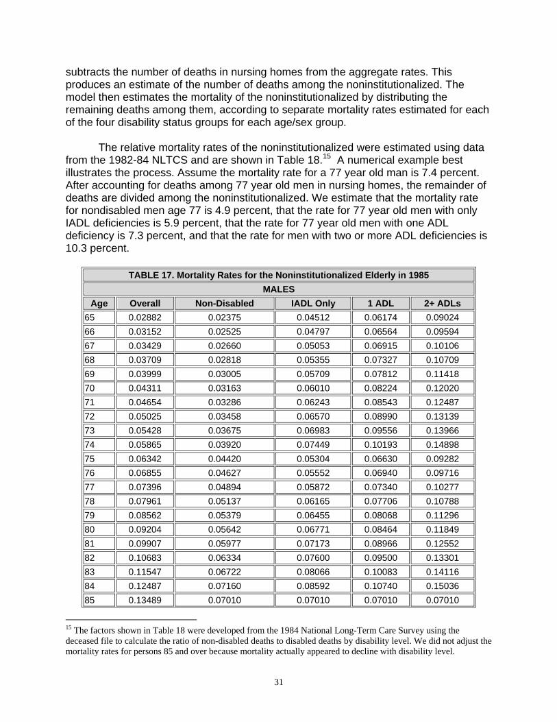
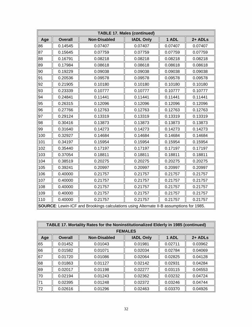
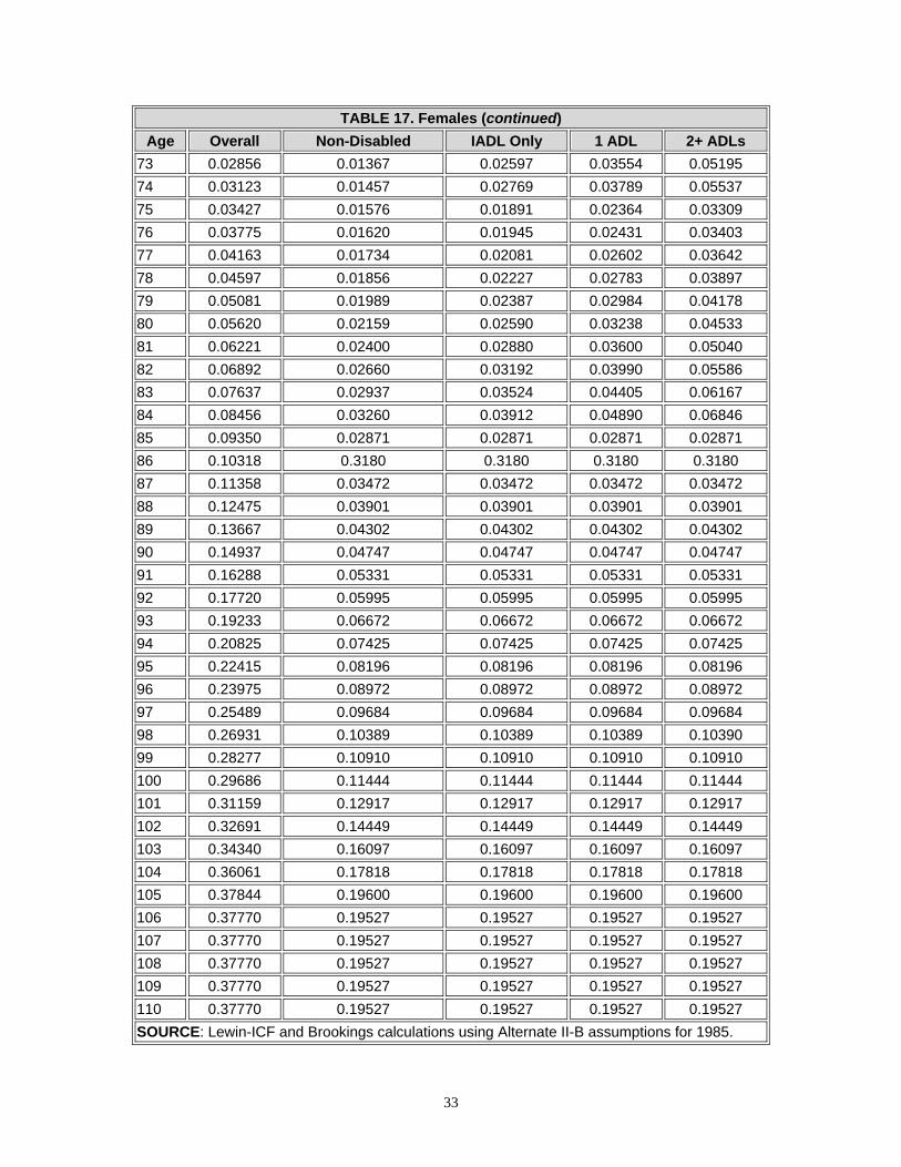
As discussed in the previous section, PRISM uses the Alternative II-B mortality assumptions from the 1988 Social Security Trustees' Report to estimate deaths for persons under age 65. Separate rates are used for disabled and nondisabled persons under age 65.

12 The 60 percent estimate is based upon SSA data (the 1982 New Beneficiary Survey) on the disability level of DI recipients. Age 62 was selected because at this age individuals become eligible for social security benefits. 13 For example, 42.2 percent of the married DI recipients who are simulated to be disabled at age 65 are assumed to have an IADL deficiency.

29

The Alternative II-B mortality assumptions are also used to determine the aggregate mortality rate by age and sex for persons age 65 and over. After individuals reach age 65, however, the model separately simulates mortality for three groups of people:

− individuals in nursing homes; − noninstitutionalized disabled individuals (IADL only, 1 ADL, and 2+ ADLs);

and − noninstitutionalized, nondisabled persons.

Different procedures are required to estimate mortality for these groups in order to account for differences in mortality across institutionalized, disabled, and nondisabled individuals.

TABLE 16. Disability Prevalence Rates for Noninstitutionalized Disability Insurance Recipients Simulated to Continue Being Disabled at Age 65a

Disability Level Married Unmarried IADL Only 42.20% 43.81% 1 ADL 19.37 23.76 2+ ADLs 38.43 32.42 Total 100.0% 100.0% a. Rates are calculated based upon the relative disability levels of 65-69 year olds by marital

status from the 1982-84 National Long Term Care Survey. Prevalence rates are expressed as percentages.

SOURCE: Brookings Institution and Lewin-ICF calculations using data from the 1982-84 National Long Term Care Survey.

1. Mortality for Institutionalized Individuals

Each institutionalized individual is assumed to survive in the nursing home

throughout the length of stay assigned by the model. As discussed below, when an individual is selected to enter a nursing home, the model uses data from the 1985 NNHS to simulate whether the individual is to be discharged alive or dead (Table 20). If the model indicates that the individual will die in the nursing home, the individual is assume d to die at the end of his or her nursing home stay.

2. Mortality for Noninstitutionalized Individuals

The model uses the Alternative II-B mortality assumptions to determine the overall mortality rate for individuals by age and sex for each year in the future. Table 17 shows these rates for 1985. The Alternative II-B assumptions include projected rates of improvement in mortality.14 The model uses these adjusted rates for future years. Once the model has determined the overall mortality rate for each age/sex group, the model 14 The model uses Social Security Trustees Alternative II-B assumptions that project improvements in mortality over time. Thus, the model's mortality rates are updated during each simulation year.

30

subtracts the number of deaths in nursing homes from the aggregate rates. This produces an estimate of the number of deaths among the noninstitutionalized. The model then estimates the mortality of the noninstitutionalized by distributing the remaining deaths among them, according to separate mortality rates estimated for each of the four disability status groups for each age/sex group.

The relative mortality rates of the noninstitutionalized were estimated using data from the 1982-84 NLTCS and are shown in Table 18.15 A numerical example best illustrates the process. Assume the mortality rate for a 77 year old man is 7.4 percent. After accounting for deaths among 77 year old men in nursing homes, the remainder of deaths are divided among the noninstitutionalized. We estimate that the mortality rate for nondisabled men age 77 is 4.9 percent, that the rate for 77 year old men with only IADL deficiencies is 5.9 percent, that the rate for 77 year old men with one ADL deficiency is 7.3 percent, and that the rate for men with two or more ADL deficiencies is 10.3 percent.

TABLE 17. Mortality Rates for the Noninstitutionalized Elderly in 1985 MALES

Age Overall Non-Disabled IADL Only 1 ADL 2+ ADLs 65 0.02882 0.02375 0.04512 0.06174 0.09024 66 0.03152 0.02525 0.04797 0.06564 0.09594 67 0.03429 0.02660 0.05053 0.06915 0.10106 68 0.03709 0.02818 0.05355 0.07327 0.10709 69 0.03999 0.03005 0.05709 0.07812 0.11418 70 0.04311 0.03163 0.06010 0.08224 0.12020 71 0.04654 0.03286 0.06243 0.08543 0.12487 72 0.05025 0.03458 0.06570 0.08990 0.13139 73 0.05428 0.03675 0.06983 0.09556 0.13966 74 0.05865 0.03920 0.07449 0.10193 0.14898 75 0.06342 0.04420 0.05304 0.06630 0.09282 76 0.06855 0.04627 0.05552 0.06940 0.09716 77 0.07396 0.04894 0.05872 0.07340 0.10277 78 0.07961 0.05137 0.06165 0.07706 0.10788 79 0.08562 0.05379 0.06455 0.08068 0.11296 80 0.09204 0.05642 0.06771 0.08464 0.11849 81 0.09907 0.05977 0.07173 0.08966 0.12552 82 0.10683 0.06334 0.07600 0.09500 0.13301 83 0.11547 0.06722 0.08066 0.10083 0.14116 84 0.12487 0.07160 0.08592 0.10740 0.15036 85 0.13489 0.07010 0.07010 0.07010 0.07010

15 The factors shown in Table 18 were developed from the 1984 National Long-Term Care Survey using the deceased file to calculate the ratio of non-disabled deaths to disabled deaths by disability level. We did not adjust the mortality rates for persons 85 and over because mortality actually appeared to decline with disability level.

31

TABLE 17. Males (continued) Age Overall Non-Disabled IADL Only 1 ADL 2+ ADLs

86 0.14545 0.07407 0.07407 0.07407 0.07407 87 0.15645 0.07759 0.07759 0.07759 0.07759 88 0.16791 0.08218 0.08218 0.08218 0.08218 89 0.17984 0.08618 0.08618 0.08618 0.08618 90 0.19229 0.09038 0.09038 0.09038 0.09038 91 0.20536 0.09578 0.09578 0.09578 0.09578 92 0.21905 0.10180 0.10180 0.10180 0.10180 93 0.23339 0.10777 0.10777 0.10777 0.10777 94 0.24841 0.11441 0.11441 0.11441 0.11441 95 0.26315 0.12096 0.12096 0.12096 0.12096 96 0.27766 0.12763 0.12763 0.12763 0.12763 97 0.29124 0.13319 0.13319 0.13319 0.13319 98 0.30416 0.13873 0.13873 0.13873 0.13873 99 0.31640 0.14273 0.14273 0.14273 0.14273 100 0.32927 0.14684 0.14684 0.14684 0.14684 101 0.34197 0.15954 0.15954 0.15954 0.15954 102 0.35440 0.17197 0.17197 0.17197 0.17197 103 0.37054 0.18811 0.18811 0.18811 0.18811 104 0.38519 0.20275 0.20275 0.20275 0.20275 105 0.39241 0.20997 0.20997 0.20997 0.20997 106 0.40000 0.21757 0.21757 0.21757 0.21757 107 0.40000 0.21757 0.21757 0.21757 0.21757 108 0.40000 0.21757 0.21757 0.21757 0.21757 109 0.40000 0.21757 0.21757 0.21757 0.21757 110 0.40000 0.21757 0.21757 0.21757 0.21757 SOURCE: Lewin-ICF and Brookings calculations using Alternate II-B assumptions for 1985.

TABLE 17. Mortality Rates for the Noninstitutionalized Elderly in 1985 (continued) FEMALES

Age Overall Non-Disabled IADL Only 1 ADL 2+ ADLs 65 0.01452 0.01043 0.01981 0.02711 0.03962 66 0.01582 0.01071 0.02034 0.02784 0.04069 67 0.01720 0.01086 0.02064 0.02825 0.04128 68 0.01863 0.01127 0.02142 0.02931 0.04284 69 0.02017 0.01198 0.02277 0.03115 0.04553 70 0.02194 0.01243 0.02362 0.03232 0.04724 71 0.02395 0.01248 0.02372 0.03246 0.04744 72 0.02616 0.01296 0.02463 0.03370 0.04926

32

TABLE 17. Females (continued) Age Non-Disabled IADL Only 1 ADL Overall 2+ ADLs

73 0.02856 0.01367 0.02597 0.03554 0.05195 74 0.03123 0.01457 0.02769 0.03789 0.05537 75 0.03427 0.01576 0.01891 0.02364 0.03309 76 0.03775 0.01620 0.01945 0.02431 0.03403 77 0.04163 0.01734 0.02081 0.02602 0.03642 78 0.04597 0.01856 0.02227 0.02783 0.03897 79 0.05081 0.01989 0.02387 0.02984 0.04178 80 0.05620 0.02159 0.02590 0.03238 0.04533 81 0.06221 0.02400 0.02880 0.03600 0.05040 82 0.06892 0.02660 0.03192 0.03990 0.05586 83 0.07637 0.02937 0.03524 0.04405 0.06167 84 0.08456 0.03260 0.03912 0.04890 0.06846 85 0.09350 0.02871 0.02871 0.02871 0.02871 86 0.10318 0.3180 0.3180 0.3180 0.3180 87 0.11358 0.03472 0.03472 0.03472 0.03472 88 0.12475 0.03901 0.03901 0.03901 0.03901 89 0.13667 0.04302 0.04302 0.04302 0.04302 90 0.14937 0.04747 0.04747 0.04747 0.04747 91 0.16288 0.05331 0.05331 0.05331 0.05331 92 0.17720 0.05995 0.05995 0.05995 0.05995 93 0.19233 0.06672 0.06672 0.06672 0.06672 94 0.20825 0.07425 0.07425 0.07425 0.07425 95 0.22415 0.08196 0.08196 0.08196 0.08196 96 0.23975 0.08972 0.08972 0.08972 0.08972 97 0.25489 0.09684 0.09684 0.09684 0.09684 98 0.26931 0.10389 0.10389 0.10389 0.10390 99 0.28277 0.10910 0.10910 0.10910 0.10910 100 0.29686 0.11444 0.11444 0.11444 0.11444 101 0.31159 0.12917 0.12917 0.12917 0.12917 102 0.32691 0.14449 0.14449 0.14449 0.14449 103 0.34340 0.16097 0.16097 0.16097 0.16097 104 0.36061 0.17818 0.17818 0.17818 0.17818 105 0.37844 0.19600 0.19600 0.19600 0.19600 106 0.37770 0.19527 0.19527 0.19527 0.19527 107 0.37770 0.19527 0.19527 0.19527 0.19527 108 0.37770 0.19527 0.19527 0.19527 0.19527 109 0.37770 0.19527 0.19527 0.19527 0.19527 110 0.37770 0.19527 0.19527 0.19527 0.19527 SOURCE: Lewin-ICF and Brookings calculations using Alternate II-B assumptions for 1985.

33

TABLE 18. Mortality Adjustments Used in the Model (Ratio of Disabled Mortality Rate to Nondisabled Mortality Rate)

Age Disability Level 65-74 75-84 85+

IADL Only 1.9 1.2 1.0 1 ADL 2.6 1.5 1.0 2+ ADLs 3.8 2.1 1.0 SOURCE: Brookings Institution and Lewin-ICF calculations using the 1982-84 National Long Term Care Survey.

34

IV. LONG TERM CARE UTILIZATION

The model simulates the utilization of long term care services for individuals based upon estimated probabilities. The use of nursing home services is simulated separately from the use of home care services. No individual can receive both types of services simultaneously, but an individual can receive more than one type of service over his or her lifetime during more than one episode and in a year when a nursing home stay lasts less than one year. A general overview of the process is provided in Figure 2. A. Nursing Home Utilization

During each year, some individuals are simulated to enter a nursing home. If an individual is selected to enter a nursing home, the model determines the length of stay and whether the individual will be discharged from the institution alive or dead. The model also determines the individual's disability level while in the nursing home and at discharge, if the individual is discharged alive.

1. Entry to Nursing Home

The model simulates the entry of individuals to nursing homes using probabilities which differ by age, sex, marital status and prior nursing home admission for the nondisabled and by age, marital status, disability level, and prior nursing home admission for the disabled.16

Nursing home entry by nondisabled persons reflects admissions by persons who

are not disabled at the beginning of the year, but become disabled and enter a nursing home at some point during the course of the year. This is more a function of the probabilities necessary for the model (i.e., nursing home entry is determined at the beginning of each year) than non-disabled people actually entering nursing homes. In fact, analysis of the 198284 NLTCS indicates that 46 percent of elderly nursing home admissions in the 1982-84 period were by persons who were not chronically disabled in 1982.17 The annual probabilities of entering a nursing home for each disability level are shown in Table 19.

The probabilities of entry in the model were estimated for individual years of age

using data from the 1982-84 National Long Term Care Survey and the 1985 National Nursing Home Survey. First, logistic models of the two year probabilities of nursing home entry were separately estimated for disabled and nondisabled persons from the 16 Sex is not used as a variable for the disabled persons because it was found not to be a statistically significant determinant of nursing home admission in the regression model developed to estimate the entry probabilities. 17 Raymond J. Hanley, Lisa Maria B. Alecxih, Joshua M. Wiener and David L. Kennell, "Predicting Elderly Nursing Home Admissions: Results from the 1982-84 National Long Term Care Survey," Research on Aging, vol.12, no.2, June 1990, pp.199-228.

35

1982-84 National Long Term Care Survey. These probabilities were then annualized and compared their predictive accuracy against a synthetic annual admission cohort estimated from the 1985 NNHS Discharge File. The annualized probabilities from the NLTCS were found to overstate admissions for those under age 85 and understate admissions for those over 85 compared to the 1985 NNHS. Therefore, the NLTCS annualized probabilities were adjusted to reflect totals from the 1985 NNHS.18 For the non-disabled with a prior nursing home admission we capped the nursing home entry probabilities at age 85 due to the small number of observations over age 85.

The probabilities used in the model implicitly assume that the rates of nursing

home admission will remain constant over time on an age/sex/marital status basis for disabled and nondisabled persons. Constant rates imply that the nursing home bed supply will increase to accommodate admissions from an increasingly large elderly population. Rates can increase based on user-specified assumptions concerning induced demand.

The model only allows individuals to enter a nursing home once each year. This is reasonable assumption because the length of stay assumptions (discussed below) reflect an aggregation of lengths of stay for persons who were discharged from nursing homes and then reentered soon thereafter.

18 To adjust the logistic nursing home entry probabilities from the 1982-84 NLTCS to approximate data from the 1985 NNHS a regression equation by age group was estimated and the coefficients were used as the adjustment factors.

36

TABLE 19. Annual Probability of Nursing Home Entry Persons with 2+ ADLs

Prior Nursing Home Stay No Prior Nursing Home Stay Age Single Married Single Married

65 12.9% 8.9% 5.2% 3.3% 66 14.0% 9.6% 5.6% 3.6% 67 15.0% 10.4% 6.1% 3.9% 68 16.2% 11.3% 6.7% 4.3% 69 17.4% 12.2% 7.2% 4.7% 70 18.6% 13.1% 7.8% 5.1% 71 20.0% 14.1% 8.4% 5.5% 72 21.3% 15.1% 9.1% 5.9% 73 22.7% 16.2% 9.8% 6.4% 74 24.2% 17.4% 10.5% 6.9% 75 25.8% 18.5% 11.3% 7.4% 76 27.4% 19.8% 12.1% 8.0% 77 29.0% 21.1% 13.0% 8.6% 78 30.7% 22.5% 13.9% 9.2% 79 32.5% 23.9% 14.9% 9.9% 80 34.3% 25.4% 15.9% 10.6% 81 36.2% 26.9% 17.0% 11.4% 82 38.2% 28.5% 18.1% 12.2% 83 40.2% 30.1% 19.3% 13.0% 84 42.3% 31.9% 20.5% 13.9% 85 44.4% 33.6% 21.8% 14.8% 86 46.6% 35.5% 23.1% 15.8% 87 48.8% 37.4% 24.5% 16.8% 88 51.1% 39.4% 26.0% 17.9% 89 53.5% 41.4% 27.5% 19.0% 90 55.9% 43.5% 29.1% 20.2% 91 58.4% 45.6% 30.7% 21.4% 92 60.9% 47.9% 32.4% 22.7% 93 63.4% 50.1% 34.2% 24.1% 94 66.1% 52.5% 36.0% 25.5% 95 68.7% 54.9% 37.9% 26.9% 96 71.4% 57.3% 39.9% 28.5% 97 74.2% 59.8% 41.9% 30.1% 98 77.0% 62.4% 44.0% 31.7% 99 79.8% 65.0% 46.2% 33.5% 100 82.7% 67.7% 48.4% 35.2% SOURCE: Lewin-ICF and Brookings Institution calculations using data from the 1982-84 National Long Term Care Survey and the 1985 National Nursing Home Survey.

37

TABLE 19. Annual Probability of Nursing Home Entry (continued)

Persons with 1 ADL Prior Nursing Home Stay No Prior Nursing Home Stay Age

Single Married Single Married 65 9.1% 6.1% 3.4% 2.2% 66 9.9% 6.6% 3.7% 2.4% 67 10.7% 7.2% 4.1% 2.6% 68 11.6% 7.8% 4.4% 2.8% 69 12.5% 8.4% 4.8% 3.1% 70 13.5% 9.1% 5.2% 3.3% 71 14.5% 9.8% 5.7% 3.6% 72 15.5% 10.6% 6.1% 3.9% 73 16.7% 11.4% 6.6% 4.2% 74 17.8% 12.2% 7.1% 4.6% 75 19.0% 13.1% 7.7% 4.9% 76 20.3% 14.1% 8.3% 5.3% 77 21.6% 15.1% 8.9% 5.7% 78 23.0% 16.1% 9.5% 6.2% 79 24.5% 17.2% 10.2% 6.6% 80 26.0% 18.3% 11.0% 7.1% 81 27.5% 19.5% 11.7% 7.6% 82 29.2% 20.8% 12.5% 8.2% 83 30.9% 22.1% 13.4% 8.8% 84 32.6% 23.4% 14.3% 9.4% 85 34.4% 24.9% 15.3% 10.0% 86 36.3% 26.4% 16.3% 10.7% 87 38.2% 27.9% 17.3% 11.5% 88 40.2% 29.5% 18.4% 12.2% 89 42.3% 31.2% 19.6% 13.0% 90 44.4% 32.9% 20.8% 13.9% 91 46.6% 34.7% 22.0% 14.8% 92 48.8% 36.6% 23.3% 15.7% 93 51.1% 38.5% 24.7% 16.7% 94 53.5% 40.5% 26.2% 17.8% 95 55.9% 42.5% 27.7% 18.9% 96 58.4% 44.7% 29.2% 20.0% 97 60.9% 46.8% 30.9% 21.2% 98 63.5% 49.1% 32.6% 22.5% 99 66.1% 51.4% 34.3% 23.8% 100 68.8% 53.8% 36.1% 25.2% SOURCE: Lewin-ICF and Brookings Institution calculations using data from the 1982-84 National Long Term Care Survey and the 1985 National Nursing Home Survey.

38

TABLE 19. Annual Probability of Nursing Home Entry (continued)

Persons with IADLs Only Prior Nursing Home Stay No Prior Nursing Home Stay Age

Single Married Single Married 65 7.8% 51.% 2.9% 1.8% 66 8.5% 5.6% 3.1% 2.0% 67 9.2% 6.1% 3.4% 2.2% 68 10.0% 6.6% 3.7% 2.3% 69 10.8% 7.2% 4.1% 2.6% 70 11.6% 7.8% 4.4% 2.8% 71 12.5% 8.4% 4.8% 3.0% 72 13.5% 9.0% 5.2% 3.3% 73 14.4% 9.7% 5.6% 3.5% 74 15.5% 10.5% 6.0% 3.8% 75 16.6% 11.3% 6.5% 4.1% 76 17.7% 12.1% 7.0% 4.5% 77 18.9% 12.9% 7.5% 4.8% 78 20.1% 13.9% 8.1% 5.2% 79 21.5% 14.8% 8.7% 5.6% 80 22.8% 15.8% 9.3% 6.0% 81 24.2% 16.9% 10.0% 6.4% 82 25.7% 18.0% 10.7% 6.9% 83 27.3% 19.2% 11.4% 7.4% 84 28.9% 20.4% 12.2% 7.9% 85 30.5% 21.6% 13.0% 8.5% 86 32.2% 23.0% 13.9% 9.1% 87 34.0% 24.4% 14.8% 9.7% 88 35.9% 25.8% 15.8% 10.4% 89 37.8% 27.3% 16.8% 11.1% 90 39.8% 28.9% 17.8% 11.8% 91 41.8% 30.5% 19.0% 12.6% 92 43.9% 32.2% 20.1% 13.4% 93 46.1% 34.0% 21.4% 14.3% 94 48.3% 35.8% 22.6% 15.2% 95 50.6% 37.7% 24.0% 16.1% 96 52.9% 39.7% 25.4% 17.1% 97 55.3% 41.7% 26.8% 18.2% 98 57.8% 43.8% 28.4% 19.3% 99 60.3% 46.0% 29.9% 20.4% 100 62.9% 48.2% 31.6% 21.7% SOURCE: Lewin-ICF and Brookings Institution calculations using data from the 1982-84 National Long Term Care Survey and the 1985 National Nursing Home Survey.

39

TABLE 19. Annual Probability of Nursing Home Entry (continued)

Non-Disabled Persons Prior Nursing Home Stay No Prior Nursing Home Stay

Males Females Males Females Age

Single Married Single Married Single Married Single Married 65 7.9% 3.0% 6.0% 2.2% 0.6% 0.2% 0.4% 0.1% 66 9.1% 3.5% 7.0% 2.6% 0.7% 0.2% 0.5% 0.2% 67 10.4% 4.1% 8.0% 3.0% 0.8% 0.3% 0.6% 0.2% 68 11.8% 4.7% 9.2% 3.5% 0.9% 0.3% 0.7% 0.2% 69 13.4% 5.4% 10.4% 4.0% 1.1% 0.4% 0.8% 0.3% 70 15.2% 6.2% 11.9% 4.7% 1.3% 0.4% 0.9% 0.3% 71 17.1% 7.2% 13.5% 5.4% 1.5% 0.5% 1.1% 0.4% 72 19.2% 8.2% 15.2% 6.2% 1.7% 0.6% 1.2% 0.4% 73 21.4% 9.3% 17.1% 7.1% 2.0% 0.7% 1.4% 0.5% 74 23.8% 10.6% 19.2% 8.1% 2.3% 0.8% 1.7% 0.6% 75 26.4% 12.1% 21.4% 9.2% 2.6% 0.9% 1.9% 0.7% 76 29.2% 13.6% 23.9% 10.5% 3.0% 1.0% 2.2% 0.8% 77 32.1% 15.4% 26.5% 11.9% 3.5% 1.2% 2.5% 0.9% 78 35.2% 17.3% 29.3% 13.4% 4.0% 1.4% 2.9% 1.0% 79 38.4% 19.4% 32.2% 15.2% 4.5% 1.6% 3.3% 1.2% 80 41.8% 21.7% 35.3% 17.1% 5.2% 1.8% 3.8% 1.3% 81 45.3% 24.1% 38.6% 19.1% 5.9% 2.1% 4.4% 1.5% 82 49.0% 26.8% 42.1% 21.4% 6.8% 2.4% 5.0% 1.8% 83 52.7% 29.7% 45.7% 23.8% 7.7% 2.8% 5.8% 2.0% 84 56.6% 32.7% 49.4% 26.5% 8.8% 3.2% 6.6% 2.3% 85 60.6% 35.9% 53.3% 29.3% 10.0% 3.6% 7.5% 2.7% 86 60.6% 35.9% 53.3% 29.3% 11.3% 4.2% 8.5% 3.1% 87 60.6% 35.9% 53.3% 29.3% 12.8% 4.8% 9.6% 3.5% 88 60.6% 35.9% 53.3% 29.3% 14.4% 5.4% 10.9% 4.0% 89 60.6% 35.9% 53.3% 29.3% 16.2% 6.2% 12.4% 4.6% 90 60.6% 35.9% 53.3% 29.3% 18.2% 7.0% 13.9% 5.2% 91 60.6% 35.9% 53.3% 29.3% 20.4% 8.0% 15.7% 5.9% 92 60.6% 35.9% 53.3% 29.3% 22.8% 9.1% 17.6% 6.7% 93 60.6% 35.9% 53.3% 29.3% 35.4% 10.3% 19.8% 7.7% 94 60.6% 35.9% 53.3% 29.3% 28.2% 11.6% 22.1% 8.7% 95 60.6% 35.9% 53.3% 29.3% 31.3% 13.1% 24.7% 9.9% 96 60.6% 35.9% 53.3% 29.3% 34.5% 14.8% 27.4% 11.1% 97 60.6% 35.9% 53.3% 29.3% 38.0% 16.6% 30.4% 12.6% 98 60.6% 35.9% 53.3% 29.3% 41.8% 18.7% 33.7% 14.2% 99 60.6% 35.9% 53.3% 29.3% 45.7% 20.9% 37.1% 16.0% 100 60.6% 35.9% 53.3% 29.3% 49.8% 23.4% 40.8% 17.9% SOURCE: Lewin-ICF and Brookings Institution calculations using data from the 1982-84 National Long Term Care Survey and the 1985 National Nursing Home Survey.

40

2. Nursing Home Length of Stay and Discharge Status

Individuals who are simulated to enter nursing homes are assigned a length of stay and a discharge status (alive or dead) based upon their age and marital status at entry. These length of stay probabilities are shown in Table 20 and are based upon lengths of stay developed from the 1985 National Nursing Home Survey Discharge File. These probabilities implicitly assume that age-group/marital status specific lengths of stay in nursing homes do not change after 1985.

There is no data set that records admissions to a nursing home and nursing home length of stay on a national basis. The 1985 National Nursing Home Survey (NNHS) is the best nationally representative data base on nursing home use, but only has a current resident survey and a discharge survey. The current resident survey reflects an average daily census for nursing homes in the U.S. The discharge survey is a sample of all the discharges from nursing homes in a year.

The 1985 National Nursing Home Discharge File was used to determine nursing home length of stay and to create a synthetic admission cohort. The synthetic admission cohort is intended to accurately represent the population entering nursing homes in 1985 by adjusting discharges for duplicate counting of individuals with more than one nursing home discharge and adjusting for the growth in the bed supply.

For the 1985 NNHS discharge file to accurately reflect an admission cohort, rather than all discharges during the year, three major problems with the NNHS Discharge File had to be addressed:

• First, the file reflects discharges not persons; because the model simulates

utilization by persons, the discharges must be related to persons; • Second, for persons with multiple discharges (i.e., discharged from one nursing

home and admitted to another, or discharged from a nursing home to a hospital and then readmitted to a nursing home) the length of stay on the file does not represent the true length of stay. Because the model simulates total length of stay within any one episode of care, the multiple discharges need to be aggregated for each individual; and

• Third, in converting discharges to admissions it is necessary to take into account

the effect of changes in the supply of nursing home beds over time on the number of long stays. This must be done to accurately reflect the likelihood of a person entering a nursing home in 1985 (if an adjustment for increases in bed supply was not made the probabilities would reflect the likelihood of entry when the bed supply was smaller).

41

TABLE 20. The Probability of Nursing Home Length of Stay by Age of Entry and Marital Statusa,b

Age of Entry 65-74 75-84 85+

Length of Stay (in days)

Live Dead Live Dead Live Dead MARRIED 1-29 21.04% 14.64% 17.25% 23.46% 16.30% 17.14% 30-59 3.91% 9.76% 8.99% 7.09% 7.95% 5.73% 60-89 2.09% 2.48% 1.76% 2.85% 3.24% 3.67% 90-179 6.61% 8.27% 3.10% 4.58% 1.59% 5.26% 180-273 3.63% 3.07% 1.92% 5.17% 1.17% 3.61% 274-364 0.83% 0.74% 0.37% 2.78% 0.00% 3.01% 365-547 0.81% 2.36% 0.56% 3.92% 2.19% 4.88% 548-729 0.32% 2.24% 0.14% 3.58% 0.31% 1.60% 730-1,094 0.69% 4.74% 0.32% 3.79% 4.23% 4.01% 1,095-1,469 0.20% 2.15% 0.82% 1.68% 0.00% 1.07% 1,470-1,824 0.67% 2.89% 0.36% 1.08% 1.35% 3.74% 1,825-2,189 0.16% 2.50% 0.00% 1.66% 0.22% 1.71% 2,190+ 0.05% 3.19% 0.39% 2.37% 0.76% 5.25% Total 40.96% 59.02% 35.99% 64.01% 39.33% 60.67% UNMARRIED 1-29 16.85% 8.21% 13.53% 9.67% 10.77% 11.73% 30-59 8.89% 2.93% 5.51% 5.48% 5.33% 5.47% 60-89 4.81% 2.52% 3.51% 2.99% 2.09% 3.89% 90-179 5.53% 4.84% 5.05% 4.16% 4.01% 7.07% 180-273 2.81% 2.46% 1.98% 4.37% 0.74% 3.93% 274-364 1.77% 1.53% 1.82% 2.15% 1.01% 4.08% 365-547 1.91% 4.09% 1.43% 5.24% 1.72% 4.49% 548-729 1.44% 2.91% 0.79% 4.67% 0.64% 4.21% 730-1,094 0.45% 5.03% 1.70% 5.32% 0.80% 7.40% 1,095-1,469 0.84% 4.16% 0.94% 4.54% 0.79% 4.87% 1,470-1,824 0.87% 1.60% 0.76% 3.86% 0.55% 4.21% 1,825-2,189 0.56% 1.70% 0.49% 2.54% 0.06% 2.25% 2,190+ 1.03% 10.24% 0.60% 6.91% 0.89% 7.03% Total 47.78% 52.22% 38.10% 61.90% 29.37% 70.63% a. “Live" and "Dead" refer to one's status at discharge. b. All probabilities are expressed as percentages. SOURCE: Brookings Institution and Lewin-ICF calculations using data from 1985 National Nursing Home Survey.

Conversion from discharges to discharged persons -- Some persons are

discharged more than once in the same year. To avoid double counting, the discharge

42

file was converted to a file of persons. In converting from discharges to persons, the last discharge during the year was assumed to be the "reference" discharge for each person. Alternatively, the first discharge in the survey year could have been used. Both methods are equally valid, but using the last discharge provides more accurate length of stay data because it allows a more accurate aggregation of discharges which have occurred previously. Specifically, in converting the file of discharges to discharged persons, two types of discharges were eliminated:

− persons who had a subsequent discharge within the survey year (to avoid double counting); and

− all discharges for individuals who had a subsequent nursing home admission within 30 days of the surveyed discharge (these individuals would either have another discharge during the survey year and therefore would be double counted or have a discharge outside the survey year and should not be included in the 1985 admission cohort).

For example, if a discharge on the Discharge File reported a subsequent discharge within the survey year, this discharge was not included in our admission cohort. With the exception of the two situations described above, all discharges were included in the admission cohort. After converting from elderly discharges to persons, the number of discharges on the 1985 NNHS file was reduced from 1,090,400 to 801,400.

Length of stay -- Although the length of stay for the reference nursing home discharge is complete, it does not capture total length of stay for persons with previous discharges. The NNHS records information on previous stays and discharge destinations. Therefore, for those with previous discharges and a re-admission within 30 days of discharge, the actual previous lengths of stay were added to the reference length of stay. The prior lengths of stay were estimated directly from the file except in two cases:

• First, for persons who report more than two previous stays, an additional third

previous stay was simulated.19 Because the length of this third previous stay was unknown, a length of stay was randomly assigned. This length of stay was based on the distribution of 1985 discharges which had a subsequent nursing home admission within 30 days of discharge but no previous stay. These discharges best approximated the length of stay of persons with a third previous stay.

• Second, an additional previous stay was imputed to persons admitted directly

from another nursing home to their "reference" discharge stay where length of stay data was unavailable for their previous stay. The length of stay distribution used was the same as for the first adjustment.

19 This was done only for persons with two previous stays in which the readmission occurred within 30 days of the discharge.

43

Cohort effect -- The 801,400 discharged persons were further adjusted to reflect the cohort effect of the growth in the nursing home bed supply. The discharge survey undercounts the number of people with long lengths of stay because there were fewer nursing home beds when people with long stays were admitted, and thus, fewer people could be admitted. Therefore, the number of people in each length of stay group was increased using a growth factor calculated from the total increase in nursing home residents from 1977 to 1985 (1.402 to 1.624 million). For example, the one to two year category was adjusted by the estimated growth in the number of beds between 1984 and 1985, the two to three year category was adjusted by the estimated growth in beds from 1983 to 1985, and so on. After this adjustment, the total number of adjusted admissions for 1985 was 824,600.

In the model, nursing home entrants are assigned a number of days within the length of stay range to which they are assigned so that the expected cross-section estimate is approximated (see Table 21).

TABLE 21. Number of Nursing Home Days Assigned by Length of Stay Category Length of Stay Category Number of Days Assigned

<30 Days 14 1-2 Months 42 2-3 Months 73 3-6 Months 129 6-9 Months 220 9-12 Months 314 1-1.5 Years 452 1.5-2 Years 634 2-3 Years 898 3-4 Years 1,257 4-5 Years 1,626 5-6 Years 1,988 6+ Years 3,619 SOURCE: Brookings Institution and Lewin-ICF calculations using data from the 1985 National Nursing Home Survey.

3. Disability Level in the Nursing Home

Once an individual enters a nursing home, the model assigns the individual a

nursing home disability level. The model assigns these disability levels because the disability status of an individual can change from the beginning of the year to the time when he or she enters a nursing home. The nursing home disability prevalence rates in Table 22 are based on the 1985 National Nursing Home Survey Current Resident File.20 The disability levels vary by age and marital status. Individuals with two or more ADLs prior to entry are assumed to continue to have this level of disability. Individuals with 20 The 1985 NNHS Current Resident File has variables indicating ADL deficiencies only.

44

lesser disabilities are assumed to have an increase in disability so that the distribution of disability of residents in the model matches the distribution of disability among residents in the 1985 NNHS. When nursing home disability status is assigned, the disability status of an individual can only increase, i.e., people's conditions do not improve at the point of entry to a nursing home.

4. Nursing Home Discharge Level of Disability

When an individual is discharged alive, he or she is then assigned a new disability level. The discharge disability level prevalence rates vary by length of stay. The prevalence rates in Table 23 were developed from the 1985 NNHS Discharge File, based on people discharged alive to the community. These people have relatively few disabilities compared to current residents because they are being discharged to home.

The 1985 NNHS Discharge File only has disability variables indicating deficiencies in mobility or continence. To categorize individuals using the three disability levels in the model, we assumed discharged residents with no deficiency in either mobility or continence were in the IADL only category; residents with a deficiency in either mobility or continence fell into the one ADL category; and residents with deficiencies in both mobility and continence were considered to have two or more ADLs.

5. Induced Demand

The model can simulate an increase in nursing home use as a result of changes in financing mechanisms. This increased use is often referred to as moral hazard or induced demand. Estimates of induced demand reflect additional admissions or increased lengths of stay as a result of new third-party payment sources.

TABLE 22. Nursing Home Disability Prevalence Rates IADL Onlya 1 ADL 2+ ADLs

Married Unmarried Married Unmarried Married Unmarried 65-69 7.8% 18.6% 6.8% 19.1% 85.5% 62.3% 70-74 5.6 13.4 8.7 14.6 85.7 72.1 75-79 5.3 11.4 9.3 13.5 85.4 75.0 80-84 7.9 8.0 5.6 14.0 86.5 78.0 85-89 3.6 6.4 10.1 11.3 86.3 82.2 90+ 3.5 4.5 2.3 10.6 94.2 84.9 a. IADL only are those who report no ADL deficiencies. SOURCE: Brookings Institution and Lewin-ICF assumptions based upon data from the 1985 National Nursing Home Survey Current Resident File.

45

TABLE 23. Nursing Home Discharge Disability Prevalence Rate Length of Stay

Less than 3 Months More Than 3 Months IADL Onlya 52.2% 40.1% 1 ADL 25.8 26.1 2+ ADLs 21.9 33.8 Total 100.0% 100.0% a. IADL only are those who report no deficiencies in either mobility or continence. SOURCE: Brookings Institution and Lewin-ICF calculations using data from 1985 National Nursing Home Survey Discharge File.

The model can estimate the effects of a given level of induced demand (user

specified) by simulating additional nursing home admissions. The model assumes these admissions are based upon the same pattern of nursing home admissions reflected in the entry probabilities in Table 19. For example, if a new public program is expected to increase nursing home entries by ten percent, the probabilities in Table 19 would be multiplied by 0.1, and those persons who had not entered a nursing home as a result of the base case probabilities would be subjected to the additional probability of nursing home entrance. These new admissions are then financed by the proposed program or simulated insurance policy. Of course, only persons who meet the requirements of the program or with insurance would enter the nursing home under the induced demand probabilities.21

Individuals who enter a nursing home due to induced demand are assumed to

have the length of stay probabilities shown in Table 24. These probabilities are based upon data from the 1985 NNHS. The disability status and mortality probabilities of individuals who enter a nursing home due to induced demand remains the same as in the base case. B. Home Care Utilization

Some individuals age 65 and over are simulated to use home care services. These services include home health care, homemaker, chore, personal care, and meal preparation services.

21 Different induced demand assumptions may be specified for persons with private insurance only, a public policy option only, or those with both private insurance and public policy options. In addition, separate induced demand assumptions may be specified for up to two insurance policies.

46

TABLE 24. The Probability of Nursing Home Length of Stay by Age of Entry and Marital Status for Persons Using Services Due to Induced Demanda

Age of Entry Length of Stay (in days) 65-74 75-84 85+

MARRIED 1-29 28.6% 32.3% 29.5% 30-59 13.1 14.0 13.6 60-89 7.8 5.4 5.1 90-179 14.3 9.6 9.1 180-364 11.1 9.1 10.0 365-729 8.2 9.9 10.4 730-1,094 5.5 4.4 5.3 1,095-1,469 3.2 2.8 4.3 1,470-1,824 2.7 2.4 4.7 1,825-2,189 1.6 3.1 1.8 2,190+ 3.9 7.0 6.2 Total 100.0% 100.0% 100.0% UNMARRIED 1-29 21.2% 19.7% 19.3% 30-59 11.7 10.7 9.5 60-89 7.0 5.4 5.5 90-179 9.6 9.8 11.5 180-364 9.1 12.1 11.8 365-729 9.1 10.8 13.2 730-1,094 7.1 7.2 7.5 1,095-1,469 4.0 6.3 5.8 1,470-1,824 2.5 4.4 4.3 1,825-2,189 3.3 3.3 2.7 2,190+ 15.4 10.3 8.9 Total 100.0% 100.0% 100.0% a. All probabilities are expressed as percentages. SOURCE: Brookings Institution and Lewin-ICF calculations using data from the 1985 National Nursing Home Survey.

As shown in Figure 3, the model simulates the use of home care services for a

number of distinct groups of the elderly:

• First, the model determines whether an individual is chronically disabled at the start of the year or whether the individual becomes chronically disabled during the year. (See Section III on disability);

• Second, the model determines which chronically disabled persons and persons

not chronically disabled at the start of the year use formal (paid) home care services;

47

• Third, the model determines the number of visits received and the period of use for users.

• Fourth, for individuals using home care, the model then determines if any visits

are Medicare-covered home health services;

• Fifth, the model determines which nonchronically disabled persons receive Medicare home health services;

The model assumes that persons in a nursing home do not use home care services while they are in a nursing home. Persons using nursing home services for part of the year may also use home care services.

1. Probability of Starting to Use Home Care for the Chronically Disabled

As discussed above and as shown in Figure 3, three groups of the elderly are simulated by the model to start using home care services in each year: 1) some persons who were chronically disabled at the start of the year; 2) some persons who were not chronically disabled at the start of the year but who become chronically disabled during the year; and 3) some persons who are not chronically disabled but use Medicare home health services as part of their recovery from an acute illness. The likelihood of starting to use home care services was estimated for each of these groups separately.

48

The likelihood of starting to use services was estimated from two data sources: 1) the 1982-84 NLTCS; and 2) Medicare program data. The 1982-84 NLTCS permits estimates of the likelihood of starting to use services for the chronically disabled; Medicare program data allows one to estimate use among the nonchronically disabled.

The 1982-84 NLTCS reports the characteristics of persons in 1982 and whether or not they used services in 1984. Unfortunately, in contrast to data in the NLTCS on nursing home use, the NLTCS does not allow one to know whether an individual used services at anytime during the 1982-84 period. Rather, it only indicates if services were being used at the time of the interview in 1984. As a consequence, the likelihood of using services in 1984 had to be estimated based upon the characteristics of individuals in 1982. These probabilities then had to be adjusted to account for persons who used services during the year but who were not receiving services on the day of the survey interview.

Separate logistic regression equations were estimated for: 1) noninstitutionalized persons who were chronically disabled in 1982; and 2) noninstitutionalized persons who were not chronically disabled in 1982 but who were chronically disabled in 1984. The equations for the noninstitutionalized disabled were estimated as a function of disability level and sex. Surprisingly, age and marital status were not significant at the 95 percent confidence level. The equation for the nondisabled was estimated as a function of age, sex, and marital status.

These equations allowed us to estimate the probability of using services in 1984 given one's characteristics in 1982 for persons who were either chronically disabled in 1982 or became chronically disabled during the 1982-84 period. However, in the model we want to simulate the start or incidence of use of services. Incidence rates were approximated using the cross-sectional data by assuming that the incidence rate was equal to the prevalence rate divided by the reported duration of use for each group of users. For example, if all users of home care in the survey had been using services for a period of two years, the incidence rate would be estimated as one-half the prevalence rate.

TABLE 25. Annual Probability of Starting to Use Formal Home Care Services for the Noninstitutionalized Chronically Disabled

Disability Level Males Females IADL Only 12.9% 22.0% 1 ADL 15.9 26.6 2+ ADLs 16.6 27.7 SOURCE: Brookings Institution and Lewin-ICF estimates based upon analysis of the 1982-84 National Long Term Care Survey.

49

TABLE 26. Annual Probability of Starting to Use Formal Home Care for Persons Who are Noninstitutionalized and Nondisabled at the Start of the Year

Males Females Age Married Single Married Single

65 1.56% 0.92% 2.14% 1.26% 66 1.69 0.99 2.31 1.37 67 1.82 1.07 2.50 1.48 68 1.97 1.16 2.70 1.59 69 2.12 1.25 2.91 1.72 70 2.29 1.35 3.14 1.86 71 2.48 1.46 3.39 2.01 72 2.67 1.58 3.66 2.17 73 2.89 1.71 3.95 2.34 74 3.12 1.85 4.26 2.53 75 3.36 1.99 4.59 2.73 76 3.63 2.15 4.95 2.95 77 3.91 2.32 5.33 3.18 78 4.22 2.51 5.75 3.43 79 4.55 2.71 6.19 3.71 80 4.91 2.92 6.67 4.00 81 5.29 3.16 7.18 4.31 82 5.70 3.41 7.73 4.65 83 6.14 3.68 8.31 5.01 84 6.61 3.96 8.94 5.40 85 7.12 4.28 9.61 5.82 86 7.66 4.61 10.33 6.27 87 8.25 4.97 11.09 6.75 88 8.87 5.36 11.91 7.27 89 9.53 5.77 12.78 7.82 90 10.25 6.22 13.70 8.42 91 11.01 6.70 14.68 9.05 92 11.81 7.21 15.72 9.73 93 12.68 7.76 16.83 10.46 94 13.59 8.35 18.00 11.23 95 14.57 8.98 19.23 12.05 96 15.61 9.65 20.54 12.93 97 16.70 10.37 21.91 13.86 98 17.86 11.14 23.35 14.86 99 19.09 11.96 24.87 15.91 100 20.39 12.83 26.46 17.02 SOURCE: Brookings Institution and Lewin-ICF estimates based on data from the 1982-84 National Long Term Care Survey.

The logit equations discussed above allowed the estimation of the prevalence

rates. Prevalence rates were divided by the reported duration of use in the 1984 NLTCS

50

to produce estimates of incidence. This procedure underestimated the number of users in 1984 by 23 percent. As a consequence, the incidence rates were multiplied by a factor of 1.23. The adjusted probabilities of starting to use home care for the chronically disabled are shown in Table 25 and Table 26. Table 25 shows estimates for persons who are disabled at the start of the year. Table 26 provides estimates for persons who are not disabled at the start of the year but who become disabled during the course of the year.

Once a chronically disabled individual is selected to receive paid home care, he or she is then assigned a disability status for the duration of his or her home care use. The disability level rates for home care users were estimated with data on users of paid home care from the 1984 NLTCS. The prevalence rates were computed as the proportion of persons in each of the disability/age/marital status groups who reported receiving paid home care on the 1984 NLTCS. Table 27 presents the paid home care disability level prevalence rates for the chronically disabled users.

2. Duration and Intensity of Service Use by the Chronically Disabled

Once the model simulates the number of chronically disabled elderly individuals who receive home care services and assigns each of them a home care disability level, it determines how long and how often they will receive home care. Disabled home care recipients' length of use was estimated from the 1982-84 NLTCS adjusted for extended episodes of home care22 (Table 28).

Once the number of months of formal home care utilization is assigned for each individual, the model estimates the number of home care visits per month based upon the disability level assigned to formal home care users. Table 29 shows these probabilities, which were estimated from the 1984 NLTCS. The model assumes that individuals in the 1-10 visits category receive 7 visits; individuals in the 11-20 visits category receive 15 visits; and persons in the 21+ visits category receive 32 visits per month.

The length of formal or informal home care use assigned to an individual may be modified by the model in two instances. First, use of home care services terminates when an individual is simulated to die. Second, use of home care also terminates upon entering a nursing home. For example, assume an individual is assigned a three year period of home care use starting in 1988 and terminating at the end of 1990 and that in 1989 the model simulates that the individual enters a nursing home for 45 days. In this instance, the individual would receive 365 days of home care in 1988. However, home care services would terminate in 1989 when the individual enters the nursing home.

22 Because the 1982-84 NLTC only provides data on how long a person has been receiving home care currently, lengths of use reported for 1984 were adjusted with data obtained from people in the survey who were home care users in both 1982 and 1984. For example, if 10 percent of the persons reporting use of home care for 3 to 6 months (4.5 months in the model) in 1982 were still using the service at the time of the interview in 1984, it was assumed in the model that 10 percent of the 1984 users with a 3 to 6 month length of use will receive care for an additional 2 years. In other words, 10 percent of the 3 to 6 month users are shifted to the 12 to 60 month duration category.

51

Thus, home care utilization in 1989 would be only 320 days (i.e., 365 less 45 days in an institution). Services would not continue into 1990. These rules apply to both formal and informal home care.

TABLE 27. Disability Level Prevalence Rates for Chronically Disabled Users of Paid Home

Care Married Unmarried

65-74 75-84 85+ 65-74 75-84 85+ IADL Only 25.2 23.9 16.7 34.1 32.3 33.9 1 ADL 18.5 20.9 16.7 24.3 25.6 37.8 2+ ADLs 56.3 55.2 66.6 41.6 42.1 28.3 Total 100.0% 100.0% 100.0% 100.0% 100.0% 100.0% SOURCE: Brookings Institution and Lewin-ICF calculations using 1982-84 NLTCS.

TABLE 28. Distribution of Home Care Length of Use for the Chronically Disabled Duration Percentage

Distribution Assigend Number of

Months of Use Less than 3 months 59.0% 2.0 3-6 months 14.2 4.5 6-12 months 9.6 9.0 12-36 months 7.1 24.0 36-60 months 7.0 48.0 More than 60 months 3.1 72.0 Total 100.0% SOURCE: Brookings Institution and Lewin-ICF calculations using data from the 1982-84 NLTCS.

TABLE 29. Monthly Number of Formal Visits by Formal Home Care Disability Levela

Formal Home Care Disability Monthly Number of Visits IADL Only 1 ADL 2+ ADLs

1-10 69.9% 59.1% 38.7% 11-20 8.4 8.0 11.8 21+ 21.7 32.9 49.5 Total 100.0% 100.0% 100.0% a. Persons selected to receive informal care are assumed to continue to use the service for the

duration of their disability. SOURCE: Brookings Institution and Lewin-ICF calculations using data from 1982-1984 National Long Term Care Survey.

Upon termination of an assigned length of home care use, an individual may

again be selected to receive home care using the probabilities presented in Table 25,

52

Table 26 and Table 31. This is also true for all individuals, including those who were discharged alive from a nursing home in a prior year. This implicitly assumes that the probability of home care utilization is the same for all individuals regardless of the individual's home care or nursing home utilization in prior years.

3. Use of Medicare Home Health Services

Some chronically disabled home care users, as well as some non- disabled persons recovering from acute illnesses, are simulated to receive Medicare home health service.

Chronically Disabled -- Based upon an analysis of the 1984 NLTCS, we estimate that 41.4 percent of the chronically disabled elderly receiving paid home care received Medicare reimbursement for some or all of their paid home care visits.

For the 41.4 percent of chronically disabled elderly home care users selected, the model then simulates the maximum number of visits covered by Medicare. Table 30 shows the probabilities of having a certain number of visits reimbursed by Medicare for persons receiving Medicare home health services. The actual number of visits covered in the model is are also shown in Table 30. The probabilities are based on Health Care Financing Administration (HCFA) data from the Medicare statistical system on the number of persons served by Medicare and the number of visits received.

TABLE 30. Medicare Reimbursed Home Health Visits Number of Reimbursed Visits Assigned Visits Probability

1-9 6 39.9% 10-20 16 23.3 21-30 27 12.1 31-40 38 7.1 41-50 49 4.6 51-99 82 8.5 100+ 165 4.1 100.0% SOURCE: Brookings Institution and Lewin-ICF calculations using Health Care Financing Administration data from the Medicare statistical system.

If the total number of visits assigned by the model for these Medicare users is

less than the maximum number covered by Medicare, all paid home care is reimbursed by Medicare. If the total number of visits is greater than the maximum number of visits covered by Medicare, the remaining visits are financed out-of-pocket, by other payers or by Medicaid.23 For example, if an individual is allowed 15 visits reimbursed by Medicare and is assigned a length of use for paid home care of less than three months, he or she

23 This is described in more detail in Section V.

53

would have 19 visits remaining after the Medicare reimbursed visits ((two months of use times 17 visits per month) -- (15 maximum covered by Medicare) = 19).

Nonchronically Disabled -- Comparison of Medicare program data and the 1984 National Long Term Care Survey data suggests that many individuals who receive Medicare home health visits are not chronically disabled and thus not included in the NLTCS sample. In order for the model simulations to agree with Medicare Program data, separate Medicare home health care use probabilities were estimated for the nonchronically disabled elderly. These probabilities, shown in Table 31, are applied to all nondisabled elderly persons who were not selected to receive paid home care with the previous set of probabilities.

If a nonchronically disabled elderly individual is selected to receive Medicare home health visits, he or she is assigned a number of visits based on probabilities shown in Table 30.

All of these visits are paid for by Medicare in the model. These users are not assigned a chronic disability level and do not receive any formal or informal home care after completing their Medicare home health episode of care.

TABLE 31. Percentage of Noninstitutionalized Non-Chronically Disabled Persons Receiving Medicare Home Health Visitsa

Age Males Females 65-74 3.06% 3.32% 75.84 4.77 4.75 85+ 9.35 16.41 a. All probabilities are presented as percentages. SOURCE: Brookings Institution and Lewin-ICF calculations using the 1982-84 NLTCS data and 1984 Medicare statistical system data.

4. Informal Care

Most disabled individuals also receive informal home care. In the model, the

prevalence rates of informal care vary by disability level and age (see Table 32). These rates were estimated from the 1982-84 NLTCS. Informal home care can be in addition to or separate from formal home care. Nondisabled individuals do not receive informal care.

54

TABLE 32. Informal Home Care Prevalence Rates for the Chronically Disabled Disability Level Age

IADL Only 1 ADL 2+ ADLs 65-74 83.5% 84.0% 95.8% 75-84 85.5 85.3 92.2 85+ 88.0 91.4 95.3 a. Persons selected to receive informal care are assumed to continue to use the service for the

duration of their disability. SOURCE: Brookings Institution and Lewin-ICF calculations using data from the 1982-1984 NLTCS.

5. Induced Demand

The model can also simulate induced demand, or increased formal home care

use, as a result of changes in financing mechanisms. The model incorporates a given level of induced demand (user specified) by simulating additional formal home care users covered by a new program of insurance. The model assumes these admissions are based upon the same pattern of formal home care use as reflected in the annual start probabilities in Table 25 and Table 26. These new home care users have their visits financed by the proposed program or simulated insurance program. For example, if a new public program is expected to increase formal home care use by ten percent, the probabilities in Table 25 and Table 26 would be multiplied by 0.1, and those persons who had not used formal home care as a result of the base case probabilities and meet the requirements of the new program or purchase insurance and meet the requirements of benefit receipt would be subjected to the additional probability.

If the new program or insurance policy has an eligibility criteria based on disability level, the disability status is used to determine whether or not an individual is subject to induced demand. The user can also specify a change in length of use. Once an individual is selected to receive induced demand formal home care, he or she is assigned a disability status for the duration of his or her home care use based on Table 27.

55

V. LONG TERM CARE FINANCING A. Nursing Home Care Financing

The model simulates nursing home expenditures and sources of payment for individuals who are institutionalized. The method of payment for nursing home services is simulated on a month-by-month basis. In each month the model estimates individuals' acute care costs and total potential expenditures for nursing home services based upon the appropriate daily rate. The model then estimates the amount paid by Medicare and out-of-pocket for these services. As individuals draw down their assets to pay for this care, the model tracks changes in each individual's eligibility for both Medicaid and Supplemental Security Income (SSI) during each month. Spousal impoverishment provisions of the 1988 Medicare Catastrophic Coverage Act are also modeled.

1. Nursing Home Charges

The model assumes that the daily charges for nursing home care vary by source of payment. As shown in Table 33, charges vary by Medicaid, Medicare, and private payer status. The Medicaid daily rate is based upon average SNF and ICF Medicaid payment rates in 1985 weighted by the number of residents receiving Medicaid skilled nursing facility (SNF) or intermediate care facility (ICF) payment in the 1985 NNHS. The private pay rate is based upon average SNF and ICF private charges in 1985 and is weighted by the total number of ICF and SNF beds in a facility. The 1985 rates were inflated to 1988 using a 7.0 percent annual increase to reflect HCFA data on nursing home price increases.

Medicare rates are based upon the average Medicare SNF per them rates estimated by the Health Care Financing Administration for the Medicare Catastrophic Coverage Act. Medicare rates are higher than Medicaid and private payer rates largely because Medicare covers only SNFs stays while the Medicaid and private payer rates include ICFs, which generally provide less intensive care than do SNFs. Medicare also reimburses a large number of hospital-based facilities, which are more expensive.

TABLE 33. Average Daily Rates for Nursing Home Care by Source of Payment

Payer Charge Per Day Assumed in Calendar Year 1988

Medicaid $55.30 Private Payer $75.90 Medicare $127.50 SOURCE: Brookings Institution and Lewin-ICF calculations using data from the 1985 National Nursing Home Facility File. Medicare estimates taken from HCFA cost estimates for the Medicare Catastrophic Coverage Act, 1988.

56

Expenditures per stay are equal to the number of days in the nursing home multiplied by the appropriate daily charge. After 1988, charges are assumed to increase at 5.5 percent a year. This projected rate of growth is based on long-run assumptions in the 1989 Trustees' Report that the consumer price index will increase at 4.0 percent per year, real wages at 1.3 percent a year and fringe benefits at 0.2 percent a year. This assumption presumes nursing home prices will continue to increase in the future to keep pace with the projected wage growth due to the heavy labor component in nursing home costs. The assumption implies that providers will need to increase wages at a rate roughly comparable to the rest of the economy in order to obtain workers and that there will be no significant productivity improvements in nursing home care in the future. As with other model assumptions, this rate of increase can be varied by the user.

2. Available Resources

The model assumes that a portion of an individual's income and assets are available to pay for nursing home expenditures and other health care costs. Available income and assets are determined as follows.

a. Available Income

In each month the model computes the amount of income available to the individual to pay for nursing home expenditures. Among single individuals, available income includes cash payments from social security; income from Individual Retirement Accounts (IRAs), Keoghs, and assets; and pensions. Individuals are assumed not to have employment earnings while in a nursing home.

For married couples, the model assumes that one-half of the couple's combined social security and asset income are available to the institutionalized spouse. Pension and IRA income and earnings from employment are assigned to the spouse who has earned the benefit or who owns the IRA.

The model also simulates intra-family transfers of income from one spouse to another. This is done in accordance with the Medicare Catastrophic Coverage Act spousal impoverishment provisions. In the case of a non-institutionalized spouse with income below 122 percent of the poverty level for a couple in 1989 (133 percent of poverty in 1990 and 150 percent in 1992), the model assumes that there is an income transfer from the institutionalized individual to the noninstitutionalized spouse of an amount sufficient to enable the noninstitutionalized spouse's income to reach the specified level of community support. The federal monthly poverty level income for elderly couples in 1990 was $653 and is assumed to increase with the CPI. Based on these calculations, the amount of income available to the individual in that month to pay for nursing home care is determined.

57

b. Acute Care Cost

Individuals who enter nursing homes generally incur other health care costs which effect the amount of income and assets individuals have available to pay for nursing home care. Acute care costs prior to admission to a nursing home are not modeled. However, after entering a nursing home, the model assumes that non-Medicaid patients have health care costs as a result of the Medicare Part B premium, and a premium for a comprehensive Medigap policy ($60 in 1989).24

Table 33 summarizes acute care costs and Medicare premiums used in the

model. The projected current law premium is the amount the elderly pay monthly for Medicare Part B coverage. The Medigap premium is a monthly approximation for other acute care costs. The Medigap policy is deflated to 1979 by the change in CPI plus two percentage points. The model uses the actual Part B premium from 1979 to 1990. After 1990, the current law premium, and the Medigap premium increase at a 5 percent inflation rate.

c. Available Assets

The entire amount of an institutionalized individual's financial (non- housing) assets less $2,000 are assumed to be available for nursing home costs. Starting in 1989, as a result of the Medicare Catastrophic Coverage Act spousal impoverishment provisions, the community spouse of a married couple may keep $12,000 or half the couple's financial/liquid assets up to $60,000, whichever is higher. The remainder less $2,000 is available to pay for institution during the year, assets are divided equally among the two patients and each may retain $2,000.

As mandated by the Deficit Reduction Act of 1984 (DEFRA), beginning in 1984, the asset limit for single individuals increased by $100 and the limit for married couples increases by $150 each year until 1989, when they equaled $2,000 and $3,000, respectively. After 1989, the asset limits for individuals are assumed to increase at 50 percent of the rate of increase in the CPI. After 1989, the asset assumptions for couples follow the Medicare Catastrophic Coverage Act spousal impoverishment rules for the spouse in the community and the DEFRA rules for individuals for the institutionalized spouse. The asset limit for married couples is assumed to increase with the CPI.

In general, home equity is assumed not to be used for nursing home expenses. However, in an effort to more closely replicate the NNHS spenddown estimates, some single nursing home patients are simulated to sell their homes to pay for care upon entry based upon the person's length of stay and whether or not the person is receiving Medicaid. For these persons, the value of their home equity is included as part of their assets to be spent for nursing home care. The assumed pattern of home sales by type of patient is shown in Table 35. 24 In 1989, additional Medicare Catastrophic premiums and the Medicare Catastrophic surtax, are also included in health care costs paids by nursing home residents.

58

TABLE 34. Medicare Part B Premium and Monthly Medigap Premiums 1989 1990 1991 1992 1993

Monthly Projected Current Law Part B Premium

$27.10 $29.00 $30.60 $32.28 $34.05

Monthly Medigap Premium $60.00 $70.00 $73.85 $77.91 $82.20 SOURCE: Congressional Budget Office, The Medicare Catastrophic Coverage Act of 1988, Staff Working Paper, August 1, 1988.

TABLE 35. Home Sale Patterns of Single Nursing Home Entrants Length of Stay Non-Medicaid Medicaid

Less than 3 months 0% 0% 3-12 months 25 5 12-24 months 50 10 24 months or more 75 15

A second parameter reduces single individuals' assets upon admission as a

proxy for asset transfer, medical expenses in the community, and allowable deductions from assets (from such items as a burial plot) based on length of stay. An arbitrarily high percentage (90 percent) of persons with low levels of financial assets ($2,000 - $5,000) is assumed to have only $2,000 in financial assets upon admission to a nursing home.25 For higher levels of assets, persons with a longer length of stay are assumed to be more likely to transfer their assets or have had medical expenses in the community. The assumed level of asset reduction is shown in Table 36.

A third parameter estimates the support received by single individuals in nursing homes from outside sources. Based upon an analysis of SIPP data, the model assumes that 10 percent of single nursing home residents who are private pay patients receive $200 per month in support from their relatives.

3. Nursing Home Care Source of Payment

The model simulates nursing home expenditures and source of payment using the nursing home charges and individual resources information described above. In each month the model simulates which individuals are eligible for Medicare and estimates the amount paid by this program. Institutionalized individuals who are either ineligible for Medicare or who exhaust their Medicare benefits are assumed to use their income and assets to pay for services. The model simulates Medicaid nursing home payments as individuals exhaust their assets and become eligible for the program.

25 That is, that Medicaid would only count $2,000 in assets.

59

TABLE 36. Probability of Reduced Assets Upon Admission to a Nursing Home Probability of Reduced Assets Asset Level

LOS <6 months LOS 6+ months Less than $5,000 90% 90% $5,000-10,000 20% 50% $10,000+ 10% 25%

a. Medicare

The model determines individual eligibility for Medicare nursing home coverage

and the level of Medicare reimbursement based on the probabilities shown in Table 37. Prior to and following 1989, the coinsurance amount for Medicare SNF benefits is one-eighth of the Part A hospital deductible for days 21 to 100, or $74 dollars per day in 1990. The first 20 days of a stay are fully covered for residents selected to receive Medicare financing.

Most individuals receive Medicare coverage for up to 30 or 45 days. Because many patients are discharged quickly, these assumptions yield an average Medicare length of stay of approximately 30 days. This is roughly equal to the average nursing home length of stay for Medicare patients during the early 1980s. In 1988, the probabilities of use and assumed days covered were increased to reflect a rising trend in Medicare SNF coverage. This increase was partly due to changes in coverage guidelines.

For 1989 (the period of the Medicare Catastrophic Coverage Act), the model assumes a dramatic increase in the percent of individuals who enter a nursing home who receive Medicare coverage. The model also assumes that ten percent of current residents receive Medicare SNF coverage in 1989 to account for the elimination of the three day prior hospitalization under MCCA. In 1989, as a result of the Medicare Catastrophic Coverage Act, Medicare paid 80 percent of the Medicare SNF rate for the first eight days of care and then covered all additional days to 150. The model applies these rules to individuals selected to be Medicare patients in 1989. The Medicare nursing home coinsurance amount for the first eight days is 20 percent (estimated to be $25.50 in 1989). The model assumes that the Medicare SNF rate, and hence, the Medicare nursing home coinsurance amount, will increase 1.5 percentage points faster than the CPI after 1986.

In 1990 and after, a relatively higher percentage of entrants and an increased days of coverage (compared to 1988) are assumed to reflect the full impact of the Medicare coverage guideline change.

60

TABLE 37. Likelihood of Receiving Medicare SNF Coverage and Length of Coverage Length of Stay Before

1988 1988 1989 1990

and After <3 months 43% 50% 60% 60% 3-6 months 27% 40% 50% 45% 6-12 months 18% 30% 35% 35% 12+ months 13% 25% 30% 30% Days of coverage 30 35 50 40 Percent of Current Residents Covered 0% 0% 50 40 SOURCE: Estimates of the distribution of Medicare coverage before 1989 are based on data from the 1985 National Nursing Home Survey Discharge File. Modifications for 1989 and 1990 and after are based on assumptions of the effects of the Medicare Catastrophic Coverage Act and changes in the Health Care Financing Administration coverage provisions.

b. Out-of-Pocket Payments

If after Medicare pays its share of an individual's nursing home care there are

remaining costs, or if the patient does not qualify for Medicare reimbursement, then the model uses the patient's resources (income and assets, in that order) to pay for nursing home services. In each month the model subtracts from a non-Medicaid patient's available income the monthly acute care costs (described above). If monthly acute care costs exceed the individual's income, the remainder is drawn from their financial assets.

The model then subtracts from available income the amount of the individual's nursing home care expenses during the month. These include any Medicare coinsurance payments in the month plus charges for nursing home days not covered by Medicare. All nursing home charges for days not covered by Medicare are based upon the private pay nursing home rates shown in Table 33. If total charges in the month are in excess of available income (after acute care expenses) the remainder is drawn from the individual's assets. Asset income in the following month is then recomputed to reflect any reduction in financial assets during the month attributed to nursing home and acute care.

c. Medicaid Payments

The model simulates an individual's eligibility for Medicaid as individuals exhaust their resources on nursing home care. Once the patient's assets are drawn down to the Medicaid assets threshold, we assume that Medicaid pays the difference between (1) the Medicaid payment rate (shown in Table 33) and (2) available income less a $30 per month personal maintenance allowance. We assume this personal maintenance allowance increases by 50 percent of the rate of change in the CPI after 1986. Once an individual become eligible for Medicaid, the individual's remaining assets are no longer drawn upon to pay for nursing home services.

61

B. Financing of Home Care Services

The model simulates expenditures and sources of payment for home care. Expenditures are equal to the number of visits multiplied by the price per visit. When the model selects a person to start receiving non-Medicare home care services or when an individual receiving Medicare home health visits exceeds the maximum number of visits covered by Medicare, the model determines eligibility and receipt of Medicaid services and if a person does not receive Medicaid financing assigns him or her to one of two remaining source of payment categories based on income.

Medicaid home care financing in the model is based on both income and asset criteria. All persons receiving Medicaid home care benefits must have assets below the SSI asset limits.26 The probability of receiving Medicaid formal home care are shown in Table 35.

The probabilities shown in Table 38 are based on information from two data sources the 1982 National Long Term Care Survey (NLTCS) and the 1984 Panel of the Survey of Income and Program Participation (SIPP). From the 1982 NLTCS the percentage of persons by source of payment (Medicaid, Out-of-Pocket, and Other Payer) and income group who were receiving non-Medicare home care was calculated. The data from the NLTCS indicate that persons with incomes up to 300 percent of poverty receive Medicaid home care visits. Unfortunately, the NLTCS data do not have reliable data on assets.

Data from SIPP was used to estimate the proportion of disabled persons in each income category who had assets below the SSI level. We used the SIPP data to increase the percentage of persons receiving Medicaid home care by income category to estimate the percentage with assets below the SSI limit who receive Medicaid.27 For example, the NLTCS reports that 14 percent of persons receiving formal non-Medicare home care with income between 100 and 200 percent of the poverty level receive Medicaid financing. SIPP indicates that 34 percent of elderly disabled persons with income between 100 and 200 percent of the poverty level have assets below the SSI level. The probability that persons in that income group would receive Medicaid financing from the NLTCS was increased by a factor of three (1/0.34) so that the aggregate proportion of persons receiving Medicaid home care in that income group would match the proportion in the NLTCS.

26 The SSI asset tests for 1989 are used for the Medicaid eligibility asset criteria ($2,000 for single persons and $3,000 for married couples). 27 The measure of disability for this analysis was any ADL or IADL impairment.

62

TABLE 38. Revised Medicaid Home Care Coverage Probabilitiesa for Persons with Assets Below SSI Level

Payment Source Single Probability Married Probability SSI Level 19% 19% SSI to Poverty 33% 33% 100-200% Poverty 44% 44% 200-300% Poverty 16% 16% a. Monthly income amounts are for 1987. Medicaid eligibility asset limits are $2,000 for single

persons and $3,000 for married persons. NOTE: Probabilities of use from the National Long Term Care Survey were adjusted to account for the percent of persons with financial assets below SSI levels based on data from the Survey of Income and Program Participation. SOURCE: Brookings Institution and Lewin-ICF estimates based on data from the 1982 National Long Term Care Survey and the 1984 Panel of the Survey of Income and Program Participation.

Persons not receiving Medicaid payments are distributed between out-of-pocket

and an other payer category by the poverty level according to the probabilities in Table 39. Other payer is a residual home care payment category that includes all funding from state and local programs, Older Americans Act and social services block grant monies, Veterans Administration programs, and charity. Individuals paying out-of-pocket for home care are assumed to use up to 30 percent of their income for services and then to use their nonhousing assets. If nonhousing assets are depleted, these individuals are assumed to return to their income to pay for services.

The prices for home care vary according to payment source. The out- of-pocket price per visit is based on data from the 1984 National Long Term Care Survey for persons who reported that they paid all home care expenses out-of-pocket; Medicare and Medicaid visit rates are based on program data average costs; and the other payer rate is a weighted average of the Medicare and out-of-pocket rates (one-third Medicare, two-thirds out-of-pocket). The charges for 1988 are shown in Table 40. The model assumes that prices increase 5.5 percent a year. Prior to 1988, prices are assumed to increase annually by two percentage points more than the CPI.

TABLE 39. Out-of-Pocket and Other Payer Home Care Financing Assignment Payment Source At or Less Than

Poverty Level Above Poverty Level

Out-of-Pocket 69.7% 86.1% Other Payer 30.3% 13.9% SOURCE: Brookings Institution and Lewin-ICF estimates based on data from the 1982 National Long Term Care Survey.

63

TABLE 40. Average Prices Per Visit for Home Care by Source of Payment in 1988 Payer Charge Per Visit in 1988

Medicaid $48,70 Medicare $51.10 Out-of-Pocket $12.50 Other $25,20 SOURCE: Brookings Institution and Lewin-ICF calculations using data from the 1982-84 NLTCS.

64

BROOKINGS/ICF LONG-TERM CARE FINANCING MODEL:

Model Assumptions

PDF Files Available for This Report Main Report http://aspe.hhs.gov/daltcp/reports/modampes.pdf ATTACHMENTS: Memos Related to Data Analysis for the Brookings/ICF Long Term

Care Financing Model http://aspe.hhs.gov/daltcp/reports/modampesA.pdf