arX

iv:1

011.

1490

v1 [

astr

o-ph

.GA

] 5

Nov

201

0

Deep Near-Infrared Survey of Dense Cores in the Pipe Nebula II: Data,

Methods, and Dust Extinction Maps

Carlos G. Roman-Zuniga1, Joao F. Alves2, Charles J. Lada3 and Marco Lombardi4

ABSTRACT

We present a new set of high resolution dust extinction maps of the nearby and essentially

starless Pipe Nebula molecular cloud. The maps were constructed from a concerted deep near-

infrared imaging survey with the ESO-VLT, ESO-NTT, CAHA 3.5m telescopes, and 2MASS

data. The new maps have a resolution three times higher than the previous extinction map of

this cloud by Lombardi et al. (2006) and are able to resolve structure down to 2600 AU. We detect

244 significant extinction peaks across the cloud. These peaks have masses between 0.1 and 18.4

M⊙, diameters between 1.2 and 5.7×104 AU (0.06 and 0.28 pc), and mean densities of about 104

cm−3, all in good agreement with previous results. From the analysis of the Mean Surface Density

of Companions we find a well defined scale near 1.4× 104 AU below which we detect a significant

decrease in structure of the cloud. This scale is smaller than the Jeans Length calculated from

the mean density of the peaks. The surface density of peaks is not uniform but instead it displays

clustering. Extinction peaks in the Pipe Nebula appear to have a spatial distribution similar to

the stars in Taurus, suggesting that the spatial distribution of stars evolves directly from the

primordial spatial distribution of high density material.

Subject headings: ISM:clouds – infrared:ISM –stars:formation

1. Introduction

A primary motivation for the study of molecular clouds at early stages of evolution is to understand

the initial conditions that precede the process of star formation. Those initial conditions are necessary to

understand the process of evolution of the clouds towards collapse into stars, and to improve numerical and

analytical experiments that should lead to a predictive model of star formation. However, there are not many

examples of clouds near or at primordial stages. That is why the Pipe Nebula is both an important and

interesting target. It is one of the youngest clouds observable, possibly magnetically dominated (Franco et al.

2010), with less than a handful of its dense cores being confirmed as currently forming stars (Onishi et al.

1999; Brooke et al. 2007; Forbrich et al. 2009). The cloud is also located at a close distance (d = 130+13−20 pc;

Lombardi et al. (2006), hereafter LAL06), offering a great level of detail to observers.

As clouds evolve, their structure is modified. The most direct way to determine the (projected) structure

of a molecular cloud is to determine the variation of an observable column density across the cloud. One

1Centro Astronomico Hispano Aleman Instituto de Astrofısica de Andalucıa (IAA-CSIC), Glorieta de la Astronomıa, S/N,

Granada, Spain, 18008

2Institute of Astronomy, University of Vienna, Turkenschanzstr. 17, 1180 Vienna, Austria

3Harvard Smithsonian Center for Astrophysics, 60 Garden Street, Cambridge MA 02138

4European Southern Observatory, Karl-Schwarzschild-Strasse 2, Garching 85748, Germany

– 2 –

method that has proven to be both reliable and accurate is to use dust extinction as a proxy for total mass

(i.e. gas column density). One successful approach to this method is the near infrared color excess technique

(Lada et al. 1994), revised and optimized by Lombardi & Alves(2001; hereafter LA01). In this technique,

stars located in the background of clouds provide individual pencil-beam measurements of reddening towards

a given line of sight. The colors of stars are averaged, weighted, and convolved into a uniform map of dust

column density using a canonical reddening law and a statistical optimization method. In their study of the

Pipe Nebula, LAL06 applied the color excess method to a sample of almost 4.5 million sources in the region

catalogued by the Two-Mass All-Sky survey (2MASS). This allowed them to construct a detailed map of

the Pipe Nebula with a spatial resolution of 1 arcminute, and an overall detection level of dust extinction

of AV = 0.5 mag. The analysis of the map revealed a large number of column density peaks, resulting in a

list of 134 candidate dense cores. The Pipe cores may also be the direct predecessors of a stellar population

with an initial mass function similar to that of the Trapezium cluster (Alves et al. 2007; Rathborne et al.

2009a, hereafter RLA09). However, while the map of LAL06 permitted a great “in bulk” view of the core

population, higher spatial resolution is needed to resolve the internal structure of the cores themselves. The

analysis of the internal structure of individual cores may help to determine their properties and their possible

stage of evolution towards collapse into stars (e.g. Lada et al. 2004). To date, such analysis has been done

for only two cores in the Pipe Nebula: Barnard 68 (Alves et al. 2001) and FeSt-1457 (Kandori et al. 2005).

This paper describes a new deep, near-infrared imaging survey of the Pipe Nebula. These new ob-

servations are 4 to 5 magnitudes deeper than 2MASS, resulting in a significant increase of the density of

background sources per unit area, allowing to construct extinction maps with higher spatial resolution and to

resolve the structure of the cloud in greater detail. The observations for this survey include data from three

ground based near-infrared facilities: the Infrared Spectrometer and Array Camera (ISAAC) at the Very

Large Telescope (VLT), the Son of Isaac (SOFI) camera at the New Technology Telescope (NTT) –both part

of the European Southern Observatory (ESO)– and the OMEGA 2000 wide field camera at the 3.5m tele-

scope at the Centro Astronomico Hispano Aleman in Calar Alto. In this paper we describe the observations

and present the data in the form of extinction maps for individual and combined fields. This paper is also a

follow up to a previous study of the structure of the Barnard 59 star forming region (Roman-Zuniga et al.

2009, hereafter Paper I), made with a subset of this survey. In this paper we pay special attention to the

nomenclature of the denser regions in the cloud: we take the conservative approach of using “extinction

peaks” to define these dense regions, as extinction peaks are the direct observables from the extinction map.

We do not call them “cores” because we have not measured radial velocity for every peak, and therefore we

cannot merge peaks into “cores”, as it was done in the analysis of RLA09.

This paper is organized as follows: in section 2 we make a general description of the observations,

and describe our data reduction process. In section 3 we present the extinction maps and describe their

construction. In section 4 we make a brief analysis of the structure in the maps and the detection of column

density peaks. In section 5 we present our results and compare them with the studies of the 2MASS map

of LAL06. Finally, a discussion and a summary of the main results are presented in sections 6 and 7,

respectively.

2. Observations and Data Reduction

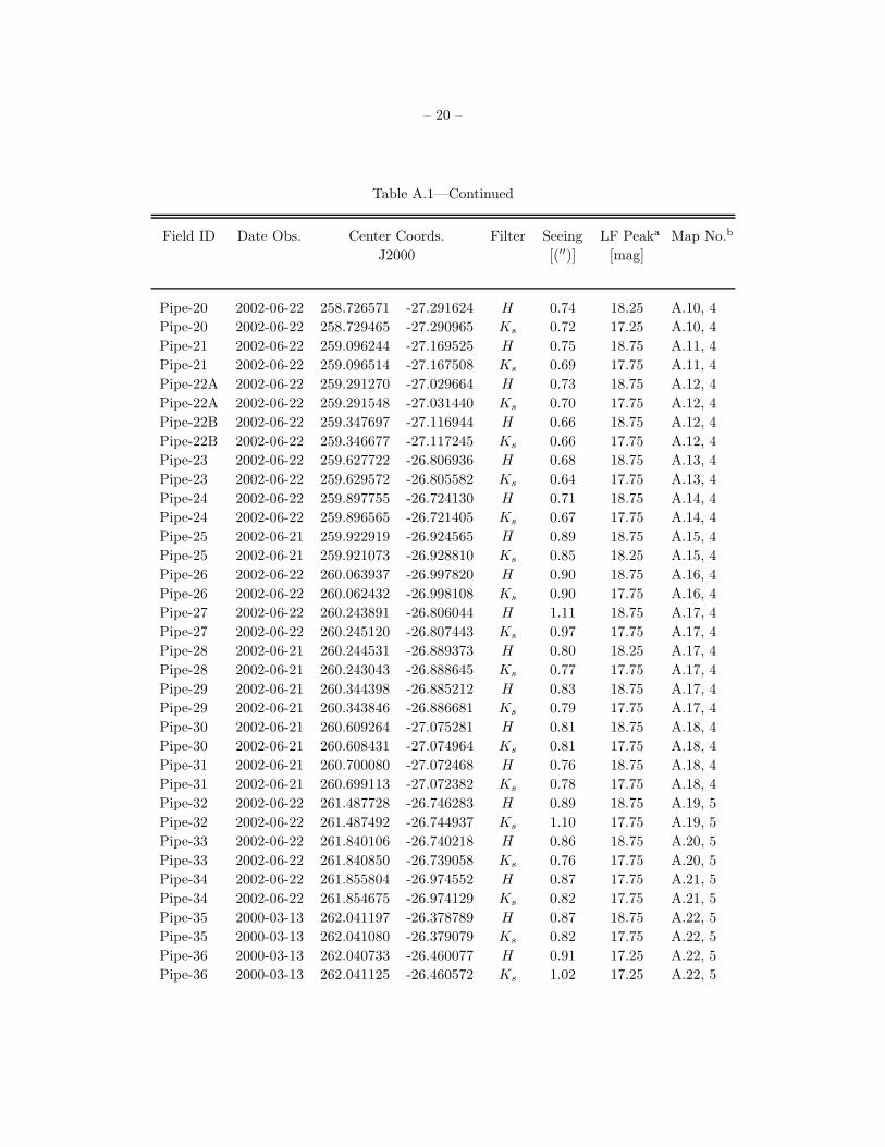
A list of all fields observed and considered for final analysis can be consulted in the Appendix (§A,

Table A.1). The table lists the field identification, the center of field positions, observation date, filter, an

estimate of the seeing based on the average FWHM of the stars detected in each field, and the peak values for

– 3 –

the brightness distributions, which are a good measurement of the sensitivity limits achieved. The location

and coverage of each field is indicated in Figure 1. In what follows we describe the observations and the

data reduction process, including the construction of the photometric catalogs used to construct the dust

extinction maps.

2.1. ESO

The main observations of the survey were made with the Infrared Spectrometer and Array Camera

(ISAAC) and the Son of ISAAC (SOFI) near-infrared imagers, mounted, respectively, at the UT3 8.2m unit

of the Very Large Telescope (VLT) array at Cerro Paranal and the 3.5m New Technology Telescope (NTT)

at La Silla, both part of the European Southern Observatory (ESO) in Chile. The two observing runs were

completed with uniformly good weather in the summer months of 2001 and 2002. Two fields, FeSt 1-457 and

B68, were observed previously in 2000 under similar conditions and requirements. All the data is currently

available at the ESO archives. The imager SOFI at the NTT 3.5m telescope, presents a field of view (FOV)

of 5′ × 5′ with plate scale of 0.288 arcsec pix−1, almost seven times the angular resolution of 2MASS, and

higher sensitivity: achieved limits are estimated to be about 4 to 5 magnitudes deeper than 2MASS in each

band. Such characteristics are enough to resolve the densely crowded Galactic Bulge field in the background

of the Pipe Nebula and to penetrate in regions with up to about 50 mag of visual extinction. The FOV of

SOFI is ample enough to allow to completely contain some of the larger dense regions in the Pipe Nebula

(R∼0.1-0.15 pc), with the exception of the central core in Barnard 59, which nearly doubles the size of the

FOV. A total of 55 fields in the cloud were successfully observed in H and Ks, with a few also observed in J .

In addition, a control field located approximately 1◦ west of Barnard 59 was observed with similar conditions

in order to determine the intrinsic background field colors, essential to determine absolute dust extinction

values. The ISAAC observations were intended to fully resolve the centers of the most dense and obscured

regions. A total of seven fields were observed with ISAAC during the same observing seasons in H and Ks

at a resolution of 0.144 arcsec pix−1 with a FOV a quarter of the size of that of SOFI. Interestingly, the

ISAAC fields observed in the center of Barnard 59 were capable of detecting only a handful of the individual

sources in and behind the core. This shows that extinction values above AV = 60 mag are close to the limit

of the penetrating power in the near-infrared even for an 8m class telescope. As mentioned before, space

based mid-infrared observations were required to resolve more of the highly obscured background sources in

B59 (Brooke et al. 2007; Roman-Zuniga et al. 2007; Paper I).

2.2. CAHA

The CAHA 3.5m observations were done with the OMEGA 2000 camera, which has a wide field of view

of 15′. A total of 21 fields, complementary to the ESO survey, were observed during june 2007 and june

2008 with acceptable weather. The fields observed with the CAHA 3.5m telescope were selected to cover

the surrounding areas in the densest region near the “Pipe Molecular Ring” (Muench et al. 2007) in the

central part of the cloud, and also to obtain fresh data in a number of fields at the westernmost regions

of the cloud (see Figure 1). The resolution of OMEGA 2000 at the 3.5m telescope is 0.45 arcsec pix−1

and the sensitivity is expected to be equivalent to that of SOFI. However, even with excellent weather

and instrumental conditions at Calar Alto, the low inclination of the Pipe Nebula at the latitude of the

observatory resulted in large seeing values (1.′′6 ± 0.2 in average) and some internal reflection effects that

affected the colors of sources near the edges of the detector. See also §3.1.

– 4 –

2.3. Pipeline Reduction

Data from the three survey groups were reduced with modified versions of the FLAMINGOS near-

infrared reduction and photometry/astrometry pipelines, which are built in the standard IRAF Command

Language environment.

One pipeline (see Roman-Zuniga 2006) processes all raw frames by subtracting darks and dividing by

flat fields, improving signal to noise ratios by means of a two pass sky subtraction method, and combining

reduced frames with an optimized centroid offset calculation.

For the ESO survey data, slight modifications were implemented to the reduction pipeline in order to

account for some –well documented– instrumental biases: For the SOFI-NTT data, we took into account

corrections for instrumental crosstalk using the IRAF task provided in the ESO SOFI webpages. Non-

linearity corrections were applied by using the coefficients listed by Tinney et al. (2003). Finally, we used

the dome flats and illumination correction field sets provided by ESO to avoid well known “shade” effects

often encountered with sky and super-sky flat fields. In the case of the ISAAC-NTT fields, master darks,

twilight flats and illumination field frames were created with the aid of the ISAAC pipelines provided in the

ESO webpages, previous to the batch reduction with our pipelines. For the Calar Alto data, the reduction

was performed using our pipeline in standard mode. We used dark frames and dome flats obtained within

48 hours of each observation. No other specific instrumental corrections were applied.

The final combined product images were then analyzed by a second pipeline, (see Levine 2006), which

identifies all possible sources from a given field using the SExtractor algorithm (Bertin & Arnouts 1996),

applies PSF photometry, calibrates observed magnitudes to a constant zero point and finds an accurate

astrometric solution. Both photometry and astrometry of SOFI and OMEGA 2000 data products were

calibrated with respect to 2MASS catalogs retrieved from the All Sky Data Release databases. ISAAC

calibrations were obtained by bootstrapping to the calibrated SOFI data. The final photometry catalogs,

containing either J , H , and Ks, or H and Ks photometry were prepared by a routine that makes use of

the routine CCXYMATCH. In the case of overlapping fields and fields with observations done in more than one

instrument, the catalogs were put together with our own matching routines, designed to list preferentially

a higher quality observation (e.g. ISAAC) over a lower quality one in the overlapping areas. We prepared

joint catalogs to construct multiple-field extinction maps for a limited number of cases. In the cases of FeSt

1-457, and SOFI fields 29, 31, and 45, we used hybrid SOFI+ISAAC catalogs.

3. High Resolution Dust Extinction Maps

The ESO and CAHA observations provide a vast enhancement in photometric depth and sensitivity

toward the fields observed. The number of sources detected in each field is up to ten times larger than

2MASS, which results in the ability to increase the spatial resolution used to map the dust column density:

with a greater source density, one can reduce the diameter of the spatial filter and have equivalent or better

statistics, with an improved signal to noise ratio.

3.1. Near Infrared Color Excess Method

The maps were constructed with the Near Infrared Color Excess Revised (NICER) technique (Lombardi & Alves

2001). NICER is an optimized multi-band technique to estimate extinction from the infrared excess cal-

– 5 –

culated from observations at three different bands –in our case J , H , and Ks, which allow to use two

independent colors. Choosing J −H and H −Ks, the estimator of the extinction, AV is of the form:

AV (s) = a+ b1[E(J −H)] + b2[E(H −Ks)] (1)

where the coefficients, a, b1 and b2 can be determined by supposing that AV is an unbiased estimator and

that it has minimum variance. The first condition is expressed as b1/C1 + b2/C2 = 1, where, in our case,

the coefficients C1 = 9.35 and C2 = 16.23 are from the reddening law of Roman-Zuniga et al. (2007). The

second condition is expressed as a+ b1(J −H)0 + b2(H −Ks)0 = 0, where (J −H)0 and (H −K)0 are the

intrinsic values of the colors, estimated from an off-cloud control field with negligible extinction (see Figure

1 and Table 1). The second condition is granted through the minimization of the variance of AV , expressed

in terms of the scatter of the intrinsic colors and the photometric errors (please see LA01 for details). We

estimated the intrinsic values of background sources in the control field as the median value along a fiducial

line represented by the average colors in bins of equal size in Ks, for Ks < 17.0 mag. The intrinsic colors

are practically constant across the control field area, with scatter comparable to or smaller than the typical

color photometric uncertainty. This is expected, because the field population towards the Galactic Bulge is

mostly composed of red giant stars, which have a very small intrinsic color dispersion in the near-infrared.

However, the source catalogs also have to be restricted to reject any stars with intrinsic color excess, like

in the case of OH IR stars, as discussed by LAL06. We selected infrared excess stars two ways: for sources

having J, H, and K photometry we selected out those falling to the right of the line H−Ks = 1.692(J−H).

For sources not having a J band observation we cannot guarantee that they will not have an intrinsic excess,

specially if H−Ks > 1. However those cases should be rare in background giant sources. For this reason, we

limited our catalogs to stars with Ks > 10.0; this restriction removes contamination from foreground stars

and most contamination from OH-IR stars (see LAL06).

To make a map, the extinction measurements for individual sources have to be spatially smoothed. In

our case, we used a Gaussian filter and Nyquist sampling. At each position (line of sight) in the map, each

star falling within the beam is given a weight calculated from a Gaussian function, and the inverse of the

variance squared. Then, the value of AV at the map position is calculated as the weighted median of all

possible values (please see LA01, sect 3.2 for details). The uncertainty in the measurement, σAV, which

determines the noise per pixel, was calculated as√

σ2(AV )/N .

We do not have ESO J band observations available for a majority of the ESO fields. Therefore, for

many ESO sources, extinction was determined from only one color, H − Ks, just as in the original color

excess technique (NICE, Lada et al. 1994). The difference is that using the NICER method we are able to

use the error associated with a measurement to keep track of its corresponding weight. For example, by

setting the photometric uncertainty of stars with no J measurement at a very large value (99.999) in that

band, NICER automatically discards that J −H measurement and either accepts or rejects a value of AV

for a star given the weight associated with the value of its H −Ks color alone.

The maps we present in this paper are constructed with a Gaussian filter with a FWHM of 20′′ and

Nyquist sampling (i.e. pixels on the map have a width of 10′′). This represents a resolution three times

higher than the one achieved in the large scale map of LAL06. This is approximately equal to 1/10 of the

median Jeans length across the cloud (0.2 pc; RLA09).

In the case of the CAHA observations we had three bands available, H , J , and Ks, thus two colors

c1 = H − Ks, c2 = J − Ks, and a pixel sampling not too different from SOFI. However, the Pipe Nebula

is a target that does not reach a very high elevation at Calar Alto, and the inclination of the telescope was

– 6 –

large enough to cause internal reflections in the camera. These reflections affected the colors of stars near

the corners of the frames. We decided to mask out the frame corners by using sources within a circular

area with a radius smaller to the diagonal length of the field. However, because each OMEGA 2000 field

contained an average of 3.5×104 detected sources, we were still able to obtain uniformly covered maps with

a very acceptable number of 15 to 60 sources per pixel and an average completeness limit of Ks = 16.75

after applying the restrictions, which was enough to resolve structures in all regions of the Pipe (with the

exception of B59) at the nominal resolution of 20′′.

3.2. Maps for Individual Fields

We constructed individual dust extinction maps for each of the SOFI and CAHA fields observed. In

the case of the few deep ISAAC fields observed, we merged the catalogs with the corresponding ones from

SOFI before proceeding to the map construction following the procedure described below. The individual

ESO and CAHA maps constitute an high resolution dust extinction map atlas of the Pipe Nebula which we

present as a separate document, accessible in the electronic (online) version of the paper. The dynamical

range of the new maps covers column densities between 1021 and 1023 cm−2.

3.3. Large Scale Maps

We merged overlapping ISAAC, SOFI and CAHA catalogs to form larger pieces which were subsequently

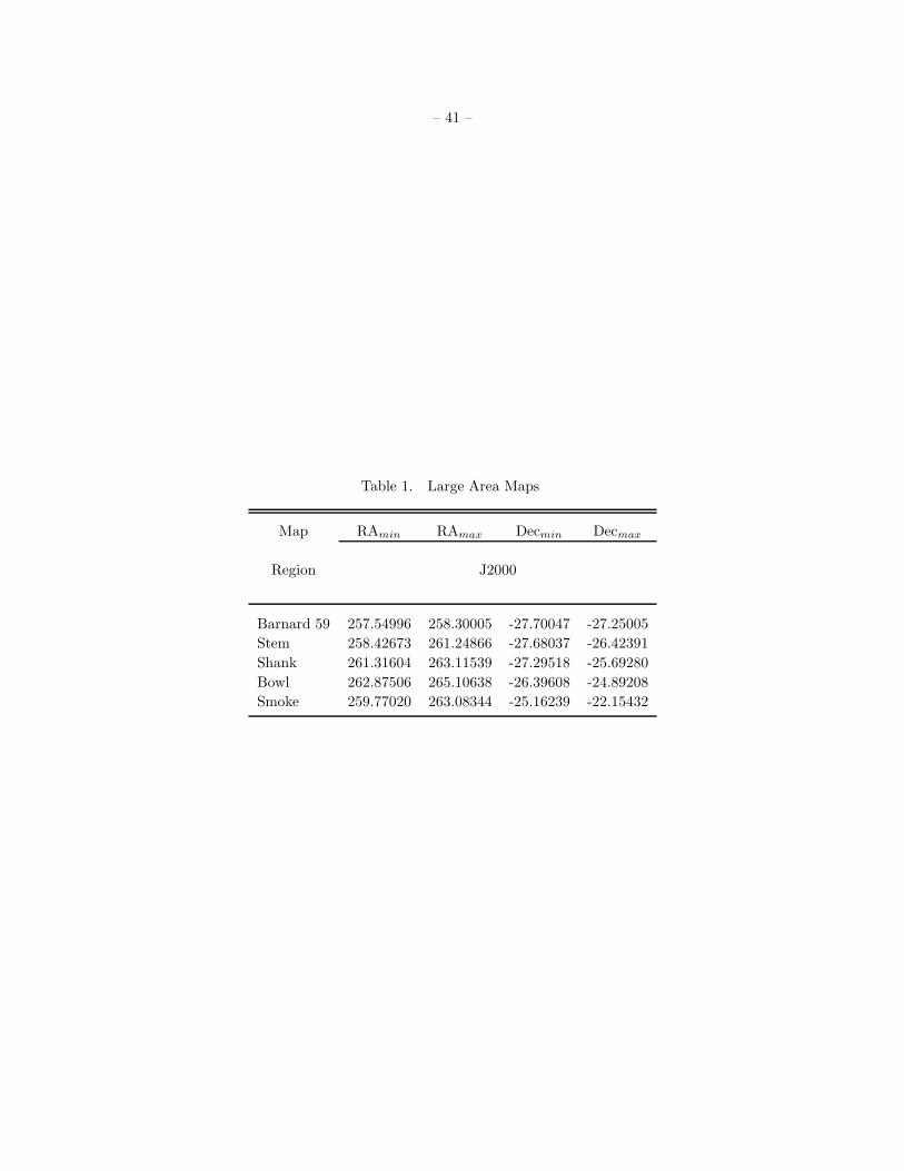
merged onto five large “bed” catalogs that defined the main regions of the cloud. This way, we constructed

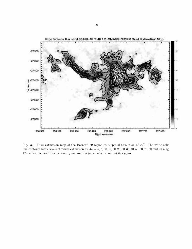
five large scale maps comprising the main regions of the Pipe –namely “Barnard 59”, “The Stem”, “The

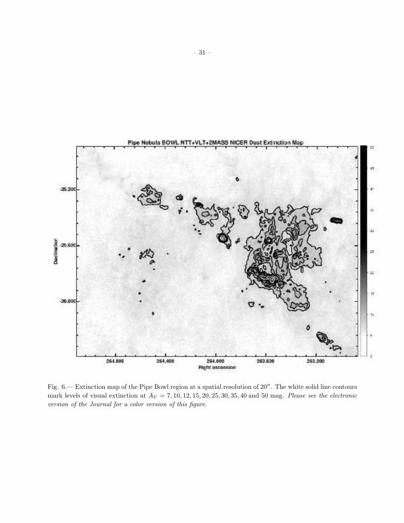
Shank”, “The Bowl” and “The Smoke”. A diagram showing the extent of each region is presented in Figure

2. The five large scale extinction maps are shown in figures 3 to 7. In Table 1 we list the limits defining

the five areas, the fields included in each one of the maps and the number of sources included from each of

the surveys. The hybrid catalogs were constructed by joining the photometry lists from the various surveys

in a progressive sequence: ISAAC catalogs were merged with the corresponding SOFI catalogs by using a

matching algorithm that preferentially listed ISAAC over SOFI detections. For those matches with a SOFI

J band detection, we used that value to replace the the null J band value from ISAAC (e.g. FeSt 1-457

field); this resulted in a small but useful reduction of the scatter as a function of extinction (σAVvs AV ).

Positional matching between NTT and VLT observations was calculated within a tolerance radius of 0.′′24, i.e.

twice the average positional uncertainty of the NTT astrometric solutions. Then, when possible, we merged

coincident ESO and CAHA fields using a slightly larger tolerance radius of 0.′′3 (to compensate for the slightly

lower resolution of the OMEGA 2000 respect to SOFI). A final “high resolution” catalog was constructed

by putting together all ESO-CAHA merges, and merging it to a 2MASS “bed” catalog obtained from the

All Sky Data Release. The 2MASS “bed” catalogs define the extent of each map, and excluded sources with

photometric flags ‘U’ and ‘X’ which indicate upper limits and defective observations, respectively. Positional

matching between the ESO-CAHA catalogs and the 2MASS bed catalogs was determined using a tolerance

radius of 0.′′36 (three times the average uncertainty of the ESO-NTT astrometric solutions), and we rejected

the 2MASS matching sources except in the cases where an ESO or CAHA source was saturated. The infrared

excess restriction applied to the 2MASS sources is the same as the one described in §3.1.

We determined that a small color correction had to be applied to correct for the differences between

the SOFI/ISAAC, OMEGA-2000 and 2MASS passbands. This correction was determined by plotting the

– 7 –

differences ∆(H −Ks) = (H −Ks)− (H −Ks)2MASS for ESO or CAHA versus (J −H)2MASS and applying

a linear least squares fit. The slopes did not vary much between ESO and CAHA fields. We estimated an

average correction of ∆(H − Ks) = −0.08 + 0.07(J − H)2MASS and applied it directly to the individual

H −Ks colors of sources entering the NICER calculations.

4. Analysis of Large Scale Maps

One of the goals of this study is to determine if the increase in resolution has any direct implications in

the determination of the structure of the cloud and the properties of identified dense regions. We also need

to determine if the increase in spatial resolution has any significant impact on our ability to identify high

column density regions. To tackle such aspects, we analyzed our maps following a technique equivalent to

that followed by LAL06 and RAL09 to analyze the 2MASS map and then compared our results to theirs.

4.1. Identification of Extinction Peaks

The maps of figures 3 to 7 show that there is abundant low density material between AV = 2 ± 1 and

AV = 6 ± 1 mag with a rough filamentary morphology. This is probably tracing a more diffuse medium,

as most significant extinction peaks appear to be embedded in these relatively large, low density structures.

The correct detection and delimitation of individual features is complicated by this aspect, because we need

to be careful at defining clearly the boundary of a feature projected against an extended emission structure.

In some cases two or more peaks are located close to each other and are projected toward the same filament

or wisp of the cloud, making it difficult to determine their individual boundaries. Because we estimate sizes

and masses of features from those boundaries, crowding and overlapping may ultimately play a crucial role in

the correct determination of a dense core mass function for the cloud, although in the Pipe Nebula, crowding

is a relatively small effect (Kainulainen et al. 2009) due to the proximity and particular layout the cloud. In

the previous studies of extinction maps of the Pipe Nebula, the detection of individual extinction peaks was

optimized in two steps: 1) filtering the local background structures and 2) extracting individual features by

means of a two-dimensional peak finding algorithm. We also follow these steps in our analysis, as described

below:

4.1.1. Filtering and Detection

The Multi-scale Vision Model algorithm (Rue & Bijaoui 1997; Bijaoui et al. 1997) translated into a

computer routine by B. Vandame (personal communication) works well for our extinction maps because it is

optimized to extract extinction peaks projected against an extended background, a picture that fits well with

a collection of dense gas cores embedded in a large cloud. The algorithm assumes that significant extinction

peaks are compact, coherent structures that will remain significant after moderate changes in resolution.

Large scale structures such as filaments and “smooth hills”, are effectively filtered out by the code as they

usually are too extended.

In our extinction maps we applied the wavelet filtering by isolating features at four scales, of sizes 2l ·sp,

where sp is the spatial resolution scale of 20′′ and l = {1, .., 4}, i.e. 0.′7, 1.′3, 2.′7, and 5.′3. At each of these

scales, the program detects local maxima among pixels with values higher than a threshold (3-sigma, in our

– 8 –

case); in the wavelet transform space, pixels associated with local maxima are organized in domains; the

program then constructs a series of trees of inter-scale connectivity, and reconstructs the image by summing

across all the scales with the help of a regularization (minimum energy loss) formulation. We checked that

the filtering at these four scales was sufficient by subtracting the filtered images from the originals. In all

cases the residual images only presented noise and some low level emission features, coincident with faint,

wispy structures visible in the large scale maps (for an example, see paper I, Fig. 5).

We identified individual extinction peaks by running the CLUMPFIND-2D (hereafter CLF2D) algorithm

(Williams et al. 1994) on the wavelet filtered maps. The algorithm detects individual peaks as local maxima

and encloses adjacent regions associated with them, defining individual boundaries or “clumps”1. The

program makes use of contour levels based on user defined intervals of constant flux. In our case, the noise

amplitude, σAV, as a function of extinction was found to be relatively uniform in the areas of low extinction

(mostly covered by 2MASS data) in the raw maps. In the Stem, Shank, Bowl and Smoke regions, the noise

level has an average value of 0.33 mag between 0.0 < AV < 30.0 mag. The noise level is lower in regions

covered by SOFI or CAHA observations), then it rises smoothly to an average of 0.55 mag as AV increases

to peak values of 40 to 50 mag per pixel (Bowl region). Following this behavior, we constructed the contour

level set with intervals starting at AV = 0.99 mag contour, defined as a “base” level equal to 3 times the

average noise per pixel in low extinction (AV < 5 mag) regions, followed by 5σAVintervals (1.65 mag) within

1 < AV < 30 mag (low and moderate extinction), and ending with 2.0 mag intervals for AV > 30. The

extra 1σ interval in the last segment is used to compensate for the increase of the noise amplitude at high

extinction regimes. This way CLF2D finds all extinction peaks in the wavelet filtered maps and works its

way down the contour levels, separating the peaks by determining which pixels most likely belong to each of

them (by means of a “friends of friends” algorithm) and finally determining the peak boundaries at the 3σ

“base” level. We restricted the detection to only include peaks enclosing a minimum of 30 contiguous pixels

with values above the “base” level; this is equivalent to saying that we only accepted as significant those

features with equivalent diameters larger than 60′′ (see below), i.e. about 1/8 of the average Jeans length

in the cloud, estimated to be ∼ 0.2 pc or 5.′3. Our choice of parameters should be considered to be on the

conservative side, but we have to take into account that the map sensitivity is lower in the regions outside

the ESO and CAHA fields, and a higher threshold helps to compensate partially for this effect.

4.1.2. Properties of Extinction Peaks

For each of the extinction peaks identified, CLF2D defines an optimized boundary. The size of a feature

is defined as the equivalent radius of the area within the boundary. Mass was estimated by summing the

background corrected total extinction in pixels within the boundary. The conversion to mass, assuming a

standard value for the gas to dust ratio NH/AV = 2.0× 1021cm−2, is given as:

Mpeak

[M]⊙= 1.28× 10−10

(

θ′′

)2 (

Dcloud

pc

)2 N∑

i=1

(AV )i M⊙, (2)

where∑N

i=1(AV )i adds the contribution of N pixels within the feature boundary in the wavelet filtered

1The word “clump” is used in a generic way by Williams et al. to describe their algorithm, but it should not be confounded

with other definitions in the literature (especially in molecular emission map analyses), in which “clumps” are considered to be

relatively large structures containing groups of cores. We avoid the use of the word “clump” in the present study.

– 9 –

map, θ is the beam size, and Dcloud is the distance to the cloud. In our case, D = 130 pc and θ = 20′′.

Using the values for mass and equivalent radii, we made estimates of the average density of the peaks,

n = 3M/4πµmHR3. Uncertainties were calculated by adding random noise to the each of the five wavelet

filtered maps (this was done following the σAVvs. AV behavior described in §4.1.1), and then running

CLF2D, to register the differences in mass and radius for all peaks that had a matched detection with the

original map. We repeated this process 25 times, and then we calculated the mean deviation from the original

values. The resultant uncertainties are 11.7%, 12.5% and 23.2% in mass, radius, and density, respectively.

Assuming a gas temperature of 10 K (consistent with estimates of TK from pointed observations of

ammonia emission by RLA09) we calculated the local Jeans length, LJ for each feature as:

LJ

[pc]= 0.2

(

T

10K

)1/2( n

104 cm−3

)−1/2

. (3)

4.1.3. Resolving higher column density structures

The depth and resolution of the 2MASS survey allowed LAL06 to produce a map with reliable column

density measurements up to a limit of AV ≈ 25 mag. One of the main goals of our high resolution survey is

to improve on this limit. Our high resolution maps now resolve the densest parts of the cloud and increase

the previous peak values by a factor of up to 4. It is important to assess how significant are these changes

for the physical characterization of the prestellar structure.

In order to assess this effect, we applied a simple unsharp masking test to the large scale maps. This

technique is frequently used in astronomical imaging to enhance or to determine the significance of detected

features (e.g. Fabian et al. (2006), Moriarty-Schieven et al. (2006)). For our maps, the masking is done in

the following manner: first we convolved the maps with a , 60′′ Gaussian beam, i.e. 3 times larger than the

nominal resolution. These smoothed images are taken as being local equivalents to the map of LAL06. Then

we subtracted these smoothed from the original images, resulting in frames with values fluctuating mostly

around zero (with both positive and negative values), except on the centers of the denser peaks, where the

residuals are relatively large and positive. We determined the mass of the residual and of the core in the 60′′

convolved maps using the formulation described in §4.1.2. The results are summarized in Figure 8, where

we plot the ratio of the masses for positionally coincident features in the residual and the low resolution

image. The ratios of the masses show clearly how the residual pixels only account, in most cases for a 5

to 30 percent of the total mass of the feature, with the larger differences being for the less massive peaks.

Thus, it is unlikely that masses of peaks in the 2MASS map of Alves et al. were underestimated significantly

because only the centers of the densest peaks were not resolved completely. Likewise, we should not expect

to find a significant number of new high extinction peaks on the high resolution maps, as the low extinction

parts of these peaks should have been easily detected in the 2MASS map.

5. Results

A total of 244 significant extinction peaks were found with our parameter restrictions within the areas

covered by the five large scale maps. All these peaks are significant in size and column density with respect

to the local background. However, we removed from the detection list seven peaks with marginal values of

size and maximum extinction because they coincide in position with extinction peaks in the 2MASS map

– 10 –

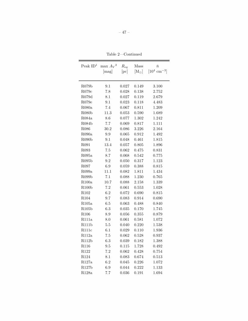
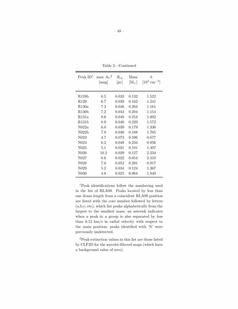
for which C18O(1-0) emission could not be detected. This leaves a total of 237 peaks for analysis. There are

36 peaks that do not have a matching position in the RLA09 list, and they are identified as new detections.

In Table 2 we list the position, size and mass for 220 peaks detected in the Stem, Shank, Bowl and Smoke

maps. The 17 remaining peaks are already listed in Table 2 of Paper I.

5.1. Global Properties

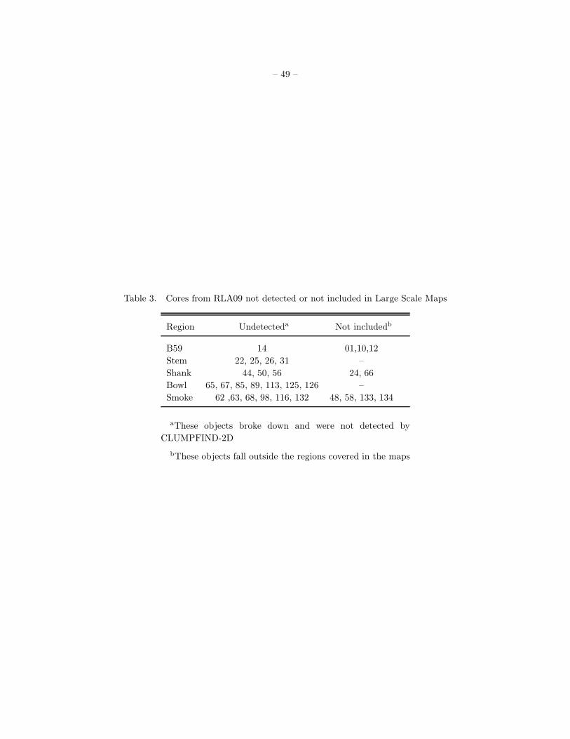
A total of 90 individual extinction peaks in our list would fall below RLA09 detection threshold. This

is equivalent to saying that about 37% of the substructure we found in the new maps is below the minimum

area threshold used by RLA09 in their analysis of the 2MASS map. This represents a significant increase in

the detection of small scale structures. We compared the diameters and separations for our list of extinction

peaks. The comparison is summarized in Figure 9, where we used astronomical units as well as pixel width

(10′′) as units of measurement. The peak to peak separations and peak diameters have median values

equivalent to 1.6 and 2.3 × 104 AU (0.08 pc and 0.11 pc), respectively, which are near half of the median

Jeans length at T = 10 K (3.7× 104 AU or 0.18± 0.05 pc). Notice that the distribution of peak separations

decreases sharply below the median value, indicating that we do not detect a significant number of extinction

peaks below that limit. We come to this point later in §5.2 and §6. The distribution of peak diameters shows

that a majority of the extinction peaks appear to have sub-Jeans sizes, but it also shows that in most

cases they are significant with respect to the minimum detection diameter of 8.3× 103 AU (0.04 pc). This

confirms that at the resolution of our maps, we are measuring structures that have dimensions below the

typical scale of thermal fragmentation for a significant number of cases. Moreover, in Figure 9 we also show,

for comparison, the detection threshold for the analysis of the 2MASS map, showing that the high resolution

of our maps resulted in an effective increase in the detection of small scale structure, which was not resolved

before.

In Figure 10 we present the mass distribution for the extinction peaks. The light colored solid curve,

is the probability density function constructed with a Gaussian kernel with a width of 0.2 in the logmass

scale. The broken, dark colored line, is the best fit for the Trapezium IMF of Muench et al. (2002) scaled

by a constant (horizontal) factor in mass. The shape of the mass distribution shows a clear departure from

a single power law at high mass. This break is above the mass completeness limit 0.2 M⊙ (see Appendix

B). Provided that each extinction peak would end up forming one star (an unlikely scenario, see §5.3 and

§6), the mass scaling factor with respect to the Trapezium IMF is 1.6± 0.1, which, following the reasoning

of Alves et al. (2007), translates into a star forming efficiency of 0.63± 0.04.

In the top panel of Figure 11 we show the mass vs. radius relationship considering all extinction peaks

detected. The least square fit to the data points show that we agree well with the power law exponent of

2.6 found by Lada et al. (2008). The bottom panel shows the distribution of mean densities; the mean value

for the extinction peaks is 1.1×104 cm−3, in good agreement with Lada et al. (2008).

5.2. Spatial Distribution

We calculated the Mean Surface Density of Companions (MSDC), Σθ, for extinction peaks. The MSDC

have been used extensively to discuss the spatial distribution of young stars in a number of regions, particu-

larly in Taurus (Gomez et al. 1993; Larson 1995; Simon 1997; Hartmann 2002; Kraus & Hillenbrand 2008).

Following Simon (1997), we determined, for a list of Npeaks peaks, the projected distances or separations,

– 11 –

θ, from each to every other feature. Then we organized them in bins (annuli) of 0.2 dex in the range

−2.0 < log θ ◦ < 2.0. Then Σθ was calculated by dividing the number of separations in each bin, Np(θ), by

the area of each annulus, and then normalizing by the total number of features. Another way to calculate

Σθ is to use the two-point correlation function (TPCF), W (θ) (Peebles 1973; Hewett 1982), which compares

the measured Σθ with that for a random, uniform distribution of points in the plane. We calculated

W (θ) =Np(θ)

Nr(θ)− 1, (4)

where Nr(θ) is the number of separations per bin for a collection of points distributed at random positions

over the same area as the survey, Amap. In our case, Amap was chosen as a rectangle of 8 × 6(◦)2 which

encloses all the regions in our maps in the RA-Dec plane. We evaluated Nr from the average of 5000 drawings

made with a Monte-Carlo routine. This way

Σθ(TPCF ) = (Npeaks

Amap)(1 +W (θ)), (5)

which can be compared with the MSDC estimated from direct counting. The results are shown in Figure

12. We see that Σθ is anti-correlated to θ, and that both estimates (MSDC and TPFC, white triangles and

black squares, respectively) are consistent with each other in the range −1.8 < log θ < 0.4 (0.04 to 5.7 pc).

The data points show that Σθ has a maximum near log θ◦ = −1.5 ≈ log θ pc = −1.1, and then it flattens

out. This break is below the median value of the local Jeans length but above our minimum detectable

size scale. This suggests that peaks are genuine substructures extending below the thermal fragmentation

length. Moreover, this maximum is equivalent to 1.45× 104 AU or 0.07 pc and it is not far from the median

of distribution of peak to peak separations (16500 AU or 0.08 pc) in figure 9. This indicates that we detect a

significant decrease in structure of the cloud at 1.45±0.2×104 AU, setting an observed limit of fragmentation

in the Pipe Nebula.

For large values of θ (log θ = 0.4 and above), the values of Σθ derived from the MSDC and the TPCF

loose consistency because the separations start to be comparable to the angular size of the map itself and

we loose information. The large “bump” near log θ = 0.5 (∼ 3◦, about 6.8 pc) in the large scale end of the

TPCF is likely a signal (somewhat diluted) from the cloud itself, which at the largest separation scales is

comparable to the size of the map. While the largest values of θ for the measured peaks are distributed

around the median length of the cloud, the random placed peaks used to calculate the TPCF are distributed

within the whole 8×6(◦)2 rectangle. We made a linear fit to the data points in the range −1.5 < log θ < 0.4.

The resultant slope is -0.91±0.04, with a correlation (Pearson) coefficient close to 1.0. This near linear

fit is indicative of a well defined power law behavior of the MSDC for prestellar condensations across the

cloud within two orders of magnitude. The linear fit and the slope near -1 are similar to values obtained

by Hartmann (2002) and Kraus & Hillenbrand (2008) for the MSDC of single stars in Taurus over a similar

range of scales.

5.2.1. Clustering of peaks?

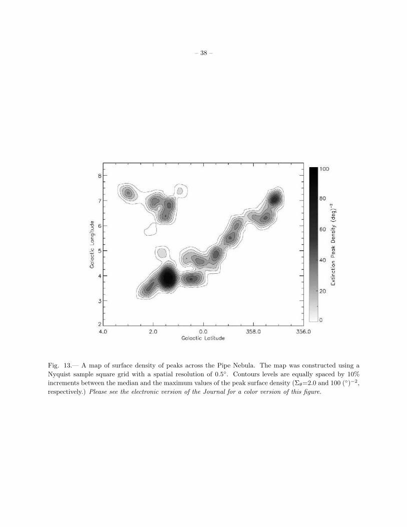
We constructed a simple map of the surface density of extinction peaks as number of peaks per square

degree, using a Nyquist sampled square grid with spatial resolution of 0.5◦. The resultant map is shown

in Figure 13. From the map, we see that the Bowl is the region with the largest density of peaks per

– 12 –

unit area, followed by B59. The Stem and the Shank regions have lower but similar total surface densities,

closer to the cloud average. The Smoke region appears to be a moderately dense region in the Pipe Nebula,

despite its peaks being less embedded. The map also shows that the surface density of extinction peaks is

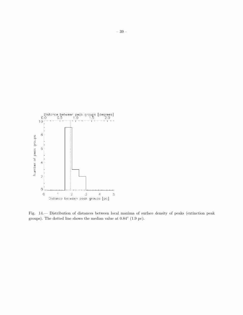
not uniform across the cloud but displays instead distinct groupings of peaks. We calculated the nearest

neighbor distance between local surface density maxima and found a very narrow distribution, with a median

value of 0.84± 0.14◦, or 1.90± 0.32 pc. The distribution is shown in Figure 14. This median distance is very

close to the expected Jeans length (2.0 pc) for a mean density of 102 cm−3 and TK = 10 K. Such values may

be typical of the more diffuse medium traced by 12CO.

5.3. Substructure or Independent Cores?

In the analysis of the 2MASS map by RLA09, they found that about 45% of the extinction peaks they

detected were separated by less than a Jeans length. They reasoned that unless large gas motions occur in the

plane of the sky, closely separated peaks with similar values of radial velocity must represent sub-structure

belonging to the same physical entity, a cloud core. Consequently they merged those extinction peaks

(about 20% of the total) which were separated by less than a Jeans length and had radial velocity differences

smaller than the one-dimensional projected sound speed in a 10K gas (δv < 0.12 km/s). This way they

obtained a final list of 134 cores out of 158 extinction peaks. Although empirical, the prescription of RLA09

is consistent with defining a core as a bounded Jeans sized region with coherent velocity (Goodman et al.

1998; Bergin & Tafalla 2007). The use of such a prescription to define a core based on a Jeans length scale

is in part justified by the fact that the global properties of these cores suggest that they are a collection of

thermally supported structures (Lada et al. 2008). In most cases the cores have thermally dominated gas

motions, as deduced from their narrow line widths (RLA09; Paper I).

In our analysis, we find that 163 out of 237 peaks are separated by their nearest neighboring peak by less

than the median Jeans Length. Based on RLA09 we know that at least a fraction of them could be grouped

into multiple peaked cores (for example, we used this information to merge some of the peaks of B59 in Paper

I). The main result of such merging is that the mass distribution function of peaks is different from the mass

distribution function of cores. Unfortunately, we do not have radial velocity information for all of the peaks

we detected in our maps, so we cannot know the total fraction of peaks that could be merged into multiple

peaked cores. For instance, in the study of RLA09 about half of sub-Jeans peaks were not close enough in

radial velocity to belong to the same core, so we could expect this to occur for a significant number of our

detections. In table 2 we used the numbering in the list of RLA09 to name those peaks separated from one

of their listed positions by less than one Jeans length, using an alphabetic subindex to identify them from

the most to the less massive. We compared this list against the list of RLA09 and found 93 peaks matching

in position, and thus having velocity information. In most cases, the C18O pointing coincided with the most

massive peak in a group. Only in a handful of cases a second peak in a group was also observed in C18O

and we were able to tell if those two peaks in the group were also close in velocity (we marked these cases

with an asterisk). However, this information is still insufficient for the majority of our peaks and we cannot

make a complete list of merged cores as in RLA09.

– 13 –

5.4. Cumulative Mass Distribution

As a cloud evolves toward star formation, an increasing fraction of material will be above a given thresh-

old extinction, at which the cloud is likely to reach the critical densities for gravitational dominance. By

comparing the cumulative mass distribution for different clouds with expected different levels of activity,

Lombardi et al. (2008) and Lada et al. (2009) showed that clouds with higher levels of high formation ac-

tivity (e.g. Ophiuchus vs. the Pipe Nebula and Orion vs. the California Nebula) also have a significantly

larger fraction of material with high column densities. While the Pipe Nebula is known to have one of the

lowest levels of star forming activity, our maps give us a good opportunity to compare the cumulative mass

distribution of the five different regions of the cloud we mapped.

In Figure 15 we plot the cumulative mass fraction as a function of extinction for each of the large scale

maps. The curves were constructed by counting the mass of the cloud above AV = 2.0 mag. The resultant

profiles for the five regions of the cloud we mapped are, indeed, very different from each other. The fraction

of the mass located at high extinction varies dramatically from the outer layers in the Smoke to the cluster

forming region in B59. For example, the fraction of pixels with values above AV = 10 mag is only over half

percent in the Smoke, the Stem and the Shank regions, but although extinction rises as high as AV ≈ 30 mag

in the Smoke (toward B68), it never reaches a level of 20 mag in the Stem-Shank transition region. At the

Bowl region the fraction of pixels with AV > 10 mag is already over 5 percent and then it is 3 times higher

at B59. Therefore, in the Pipe Nebula the fraction of high density material appears to be directly related

to the condensation of the material toward star formation. Our data shows that a significant increase in the

fraction of high extinction material as star formation is onset, is not only noticeable from cloud to cloud,

but within regions in the same cloud. Moreover, the cumulative mass fraction in the Pipe Nebula appears

to vary significantly even though its global star formation rate is low.

6. Discussion

One of the main goals of this paper is to take advantage of the higher spatial resolution achieved and

determine the structure of the cloud across a larger range of spatial scales. From the analysis of the MSDC

presented in section 5.2, we see that the Pipe Nebula presents correlated dense structure between 1.45× 104

AU (0.07 pc) and 1.48×106 AU (7.2 pc). The function Σθ appears to break below the former scale, indicating

a significant decrease in structure of the cloud. This is consistent with the sharp decrease of the number of

extinction peaks with diameters below 1.65× 104 AU (0.08 pc; see Fig. 9). This possible limit for the scale

of fragmentation is also consistent with a recent study by Schnee et al. (2010) who, using interferometric

radio continuum observations, found no evidence of fragmentation in cores of the Perseus Molecular Cloud

at scales of 103 − 104 AU. Also, this break in the slope of the MSDC for extinction peaks appears at a scale

that is smaller than the Jeans length in the cloud, 4.1× 104 AU (0.2 pc). A thermal fragmentation scale is

expected to be relevant in a cloud like the Pipe, where it has been found that gas motions inside cores are

mostly thermal and subsonic (Lada et al. 2008), so it is worth discussing some of the possible scenarios in

which a significant amount of structure below the thermal fragmentation length could have formed.

One possibility is that the cloud is presenting a self-similar structure where as we increase the spatial

resolution of our maps, the amount of structure also increases. We do observe a self-similar behavior within

a range of spatial scales, as shown in Fig. 12. However, we observe that this behavior is truncated at scales

below 0.07 pc, defining an intrinsic length in the cloud fragmentation process. The slope near -1 in the

MSDC of extinction peaks in the Pipe Nebula is similar to the one obtained in the analysis of the MSDC for

– 14 –

single stars in Taurus by Hartmann (2002). They suggested that a slope near -1 could reflect the distribution

of peaks along the filamentary structure of the cloud, and not necessarily a self-similar structure of the cloud.

A second possibility is that the thermal fragmentation scale is smaller than that given from equation

3 for the median density of peaks. In order to match the Jeans length defined in equation 3 with the

observed scale of fragmentation –assuming the estimates of temperature ∼ 10K from ammonia observations

by Rathborne et al. (2008)–, peaks would need to have densities about 6.3 times larger than those we derive.

Likewise, if we assume the densities are correct, then the dense regions in the cloud would have to be as cold

as 5 K. Both of this possibilities are unlikely.

A third possibility is that the main filament of the Pipe Nebula is inclined by a large angle with respect

to the plane of the sky, reducing the projected separations between peaks. However, a discrepancy of a factor

of 2 would require the filament to be inclined by about 60◦, which seems unlikely. However, a similar effect

could be caused by the overlap of distinct regions of the cloud along the same line of sight, and this would

be difficult to rule out.

A fourth possibility is that a significant fraction of peaks separated by less than the Jeans length could

belong to the same core, as found in RLA09. In that case, such peaks would represent substructure in multiple

peaked cores. It could be possible that cores with multiple peaks are similar in nature to the Globule 2 in

the Coalsack, a relatively massive (6 M⊙) core that is characterized by a ring-like (sub-Jeans) structure

(Lada et al. 2004) that appears to be the product of two converging subsonic flows of gas (Rathborne et al.

2009b), and thus in a very early stage of evolution. However we do not have sufficient data to asses how

large this effect could be across the cloud.

Another result of this study is that the analysis of the MSDC shows that individual extinction peaks are

spatially distributed along the Pipe Nebula cloud in a similar fashion as single stars in the Taurus molecular

cloud. At large scales, our data shows that peaks in the Pipe are distributed in small groups across the

cloud, in a similar fashion to stars distributed in small clusters in Taurus (Gomez et al. 1993). The typical

separation between groups may be consistent with the Jeans length for ta more diffuse medium. Thus, our

data could be evidence of thermal fragmentation of the cloud at two spatial scales, one defined by material

with densities near 100 cm−3, and the other one defined by material with densities near 104 cm−3. The

distribution of peaks is essentially similar to the distribution of stars in Taurus. Our results suggest that the

spatial distribution of the stars may evolve directly from the primordial distribution of dense cloud material.

7. Summary

1. This article describes a sensitive, high resolution, near-infrared survey of selected high extinction fields

in the Pipe Nebula. The aim of the survey is to resolve the structure of individual high density regions

and their local environment.

2. The near-infrared data was used to construct extinction maps for individual fields using the NICER

color excess technique. We merged our deep, high resolution photometry catalogs with data from the

2MASS survey and made five large scale maps corresponding to the main regions of the cloud: B59

(discussed separately in Paper I), the Stem, the Shank, the Bowl, and the Smoke.

3. The new extinction maps have a spatial resolution of 20′′, three times higher than the one achieved in

the 2MASS map of LAL06, and enable us to resolve structure down to 2600 AU.

4. We detect 244 significant extinction peaks above a more diffuse background. This number of peaks is

– 15 –

larger than that found in the map of Lombardi et al (201 peaks). In particular, 90 peaks were found

below the detection threshold of that previous survey and contribute to define a new lower completeness

limit for extinction features in the Pipe Nebula.

5. The distribution of peak to peak separations has a median value of 0.08 pc, which is coincident with

a maximum value for the two-point correlation function and the mean surface density of companions

near 14500 AU (0.07 pc), marking a scale below which we observe a significant decrease in the structure

of the cloud.

6. The extinction peaks have masses between 0.1 and 18.4 M⊙, diameters between 0.06 and 0.28 pc, and

mean densities near 1.0×104 cm−3, in good agreement with previous studies. The mean diameter of

these extinction peaks is about half the Jeans length for this cloud.

7. The cumulative mass fraction of pixels as a function of extinction, exhibits significant differences for

separate regions in the cloud, with the cluster forming region B59 having a significantly larger fraction

of material with high column densities. This shows that a significant increase in the fraction of high

extinction material as star formation is onset, is not only noticeable from cloud to cloud, but within

regions in the same cloud.

8. The mean surface density of companions for peaks in the Pipe Nebula is similar to the one obtained

for single stars in Taurus. In addition, the surface density of the peaks is not uniform, but instead it

displays several local maxima across the cloud, showing that the peaks may form small clusters, like

the stars in Taurus. Our data suggests that the spatial distribution of stars we see in clouds like Taurus

may evolve directly from a primordial spatial distribution of density peaks.

We want to thank an anonymous referee for a comprehensive review of the manuscript, which resulted

in a significant improvement of the content. We want to acknowledge Benoit Vandame for providing a code

to produce the wavelet filtered maps, and for his very illustrative tutorials on the topic. We acknowledge

fruitful discussions with Doug Johnstone (specially on unsharp masking), Jill Rathborne (who kindly shared

information on C18O observations), August Muench, Nestor Sanchez, Miguel Cervino and Paula Teixeira,

as well as discussions with the participants of the “Pipe Nebula State of the Union” workshop that took

place in Granada in May 2009. This project acknowledges support from NASA Origins Program (NAG

13041), NASA Spitzer Program GO20119 and JPL contract 1279166. Carlos Roman-Zuniga acknowledges

support from a Calar Alto Post-doctoral Fellowship. Joao Alves thanks a starting research grant from the

University of Vienna. We acknowledge the help of Paranal Observatory, La Silla Observatory, and Calar

Alto Observatory science operation teams for assistance during observations. Data in this publications is

based on observations collected at the Centro Astronomico Hispano Aleman (CAHA), operated jointly by the

Max-Planck Institut fur Astronomie and the Instituto de Astrofısica de Andalucıa (CSIC). This publication

makes use of data products from the Two Micron All Sky Survey, which is a joint project of the University of

Massachusetts and the Infrared Processing and Analysis Center/California Institute of Technology, funded

by the National Aeronautics and Space Administration and the National Science Foundation.

Facilities: NTT (SOFI), VLT:Melipal (ISAAC), CAHA:3.5m (OMEGA 2000)

REFERENCES

Alves, J., Lombardi, M., & Lada, C. J. 2007, A&A, 462, L17

– 16 –

Alves, J. F., Lada, C. J., & Lada, E. A. 2001, Nature, 409, 159

Bergin, E. A. & Tafalla, M. 2007, ARA&A, 45, 339

Bertin, E. & Arnouts, S. 1996, A&AS, 117, 393

Bijaoui, A., Rue, F., & Vandame, B. 1997, in Data Analysis in Astronomy IV, ed. V. Di Gesu, M. J. B.

Duff, A. Heck, M. C. Maccarone, L. Scarsi, & H. U. Zimmerman, 337

Brooke, T. Y., Huard, T. L., Bourke, et al. 2007, ApJ, 655, 364

Fabian, A. C., Sanders, J. S., Taylor, G. B., Allen, S. W., Crawford, C. S., Johnstone, R. M., & Iwasawa,

K. 2006, MNRAS, 366, 417

Franco, G. A. P., Alves, F. O., & Girart, J. M. 2010, ApJ, 723, 146

Forbrich, J., Lada, C. J., Muench, A. A., Alves, J., & Lombardi, M. 2009, ApJ, 704, 292

Gomez, M., Hartmann, L., Kenyon, S. J., & Hewett, R. 1993, AJ, 105, 1927

Goodman, A. A., Barranco, J. A., Wilner, D. J., & Heyer, M. H. 1998, Astrophysical Letters Communica-

tions, 37, 109

Hartmann, L. 2002, ApJ, 578, 914

Hewett, P. C. 1982, MNRAS, 201, 867

Kainulainen, J., Lada, C. J., Rathborne, J. M., & Alves, J. F. 2009, A&A, 497, 399

Kandori, R., Nakajima, Y., Tamura, M., Tatematsu, K., Aikawa, Y., Naoi, T., Sugitani, K., Nakaya, H.,

Nagayama, T., Nagata, T., Kurita, M., Kato, D., Nagashima, C., & Sato, S. 2005, AJ, 130, 2166

Kraus, A. L. & Hillenbrand, L. A. 2008, ApJ, 686, L111

Lada, C. J., Huard, T. L., Crews, L. J., & Alves, J. F. 2004, ApJ, 610, 303

Lada, C. J., Lada, E. A., Clemens, D. P., & Bally, J. 1994, ApJ, 429, 694

Lada, C. J., Muench, A. A., Rathborne, J., Alves, J. F., & Lombardi, M. 2008, ApJ, 672, 410

Lada, C. J., Lombardi, M., & Alves, J. F. 2009, ApJ, 703, 52

Larson, R. B. 1995, MNRAS, 272, 213

Levine, J. 2006, PhD thesis, University of Florida

Lombardi, M. & Alves, J. 2001, A&A, 377, 1023

Lombardi, M., Alves, J., & Lada, C. J. 2006, A&A, 454, 781

Lombardi, M., Lada, C. J., & Alves, J. 2008, A&A, 489, 143

Moriarty-Schieven, G. H., Johnstone, D., Bally, J., & Jenness, T. 2006, ApJ, 645, 357

Muench, A. A., Lada, E. A., Lada, C. J., & Alves, J. 2002, ApJ, 573, 366

Muench, A. A., Lada, C. J., Rathborne, J. M., Alves, J. F., & Lombardi, M. 2007, ApJ, 671, 1820

– 17 –

Onishi, T., Kawamura, A., Abe, R., Yamaguchi, N., Saito, H., Moriguchi, Y., Mizuno, A., Ogawa, H., &

Fukui, Y. 1999, PASJ, 51, 871

Peebles, P. J. E. 1973, ApJ, 185, 413

Rathborne, J. M., Lada, C. J., Muench, A. A., Alves, J. F., Kainulainen, J., & Lombardi, M. 2009a, ApJ,

699, 742

Rathborne, J. M., Lada, C. J., Muench, A. A., Alves, J. F., & Lombardi, M. 2008, ApJS, 174, 396

Rathborne, J. M., Lada, C. J., Walsh, W., Saul, M., & Butner, H. M. 2009b, ApJ, 690, 1659

Roman-Zuniga, C. G. 2006, PhD thesis, University of Florida

Roman-Zuniga, C. G., Lada, C. J., & Alves, J. F. 2009, ApJ, 704, 183

Roman-Zuniga, C. G., Lada, C. J., Muench, A., & Alves, J. F. 2007, ApJ, 664, 357

Rue, F. & Bijaoui, A. 1997, Experimental Astronomy, 7, 129

Schnee, S., Enoch, M., Johnstone, D., Culverhouse, T., Leitch, E., Marrone, D. P., & Sargent, A. 2010, ApJ,

718, 306

Simon, M. 1997, ApJ, 482, L81+

Tinney, C. G., Burgasser, A. J., & Kirkpatrick, J. D. 2003, AJ, 126, 975

Williams, J. P., de Geus, E. J., & Blitz, L. 1994, ApJ, 428, 693

This preprint was prepared with the AAS LATEX macros v5.2.

– 18 –

A. Summary of Observations

– 19 –

Table A.1. Near-Infrared Observations of Pipe Nebula Fields

Field ID Date Obs. Center Coords. Filter Seeing LF Peaka Map No.b

J2000 [(′′)] [mag]

SOFI-NTT OBSERVATIONS

B59-01 2002-06-20 257.631573 -27.426578 H 0.86 19.25 A.1, 3

B59-01 2002-06-20 257.626906 -27.428854 Ks 0.81 18.50 A.1, 3

B59-02 2002-06-20 257.722044 -27.431189 H 1.00 19.25 A.2, 3

B59-02 2002-06-20 257.723116 -27.431726 Ks 0.93 18.25 A.2, 3

B59-03 2002-06-20 257.721593 -27.459140 H 0.90 18.75 A.3, 3

B59-03 2002-06-20 257.719551 -27.460034 Ks 0.85 17.75 A.3, 3

B59-04 2001-06-09 257.934286 -27.432649 H 1.06 18.75 3

B59-04 2001-06-09 257.935579 -27.433704 Ks 1.09 18.25 3

B59-05 2002-06-20 257.799520 -27.470299 H 0.84 19.75 3

B59-05 2002-06-20 257.803101 -27.472615 Ks 0.84 18.75 3

B59-06 2002-06-20 257.914017 -27.374625 H 0.89 19.75 3

B59-06 2002-06-20 257.914131 -27.375762 Ks 0.83 18.75 3

B59-07 2002-06-20 257.910182 -27.469140 H 0.80 19.75 3

B59-07 2002-06-20 257.910421 -27.467422 Ks 0.78 18.25 3

B59-08 2002-06-20 257.909318 -27.550688 H 0.85 19.25 A.4, 3

B59-08 2002-06-20 257.916099 -27.550724 Ks 0.76 18.75 A.4, 3

B59-09 2002-06-20 258.066477 -27.621523 H 0.95 18.75 A.5, 3

B59-09 2002-06-20 258.068466 -27.623340 Ks 0.84 18.25 A.5, 3

B59-10 2002-06-20 257.986905 -27.426153 H 0.85 19.75 A.6, 3

B59-10 2002-06-20 257.987585 -27.423171 Ks 0.79 18.25 A.6, 3

B59-11 2002-06-20 258.073628 -27.410908 H 0.84 19.25 A.6, 3

B59-11 2002-06-20 258.073722 -27.411663 Ks 0.82 18.25 A.6, 3

B59-12 2002-06-20 258.138957 -27.340032 H 0.84 19.25 A.6, 3

B59-12 2002-06-20 258.139848 -27.339383 Ks 0.79 18.25 A.6, 3

B59-13 2002-06-21 258.220558 -27.391059 H 0.97 18.75 A.7, 3

B59-13 2002-06-21 258.219609 -27.392223 Ks 0.91 18.25 A.7, 3

Pipe-16 2002-06-22 258.815340 -27.557691 H 0.88 18.25 A.8, 4

Pipe-16 2002-06-22 258.815775 -27.558311 Ks 0.77 17.75 A.8, 4

Pipe-17 2002-06-22 258.943817 -27.503255 H 0.98 18.75 A.9, 4

Pipe-17 2002-06-22 258.942134 -27.502738 Ks 0.81 17.75 A.9, 4

Pipe-18 2002-06-22 259.021660 -27.517372 H 0.84 18.25 A.9, 4

Pipe-18 2002-06-22 259.020609 -27.517635 Ks 0.78 17.75 A.9, 4

Pipe-19 2002-06-22 258.743043 -27.368822 H 0.87 18.25 A.10, 4

Pipe-19 2002-06-22 258.742166 -27.369409 Ks 0.88 17.75 A.10, 4

– 20 –

Table A.1—Continued

Field ID Date Obs. Center Coords. Filter Seeing LF Peaka Map No.b

J2000 [(′′)] [mag]

Pipe-20 2002-06-22 258.726571 -27.291624 H 0.74 18.25 A.10, 4

Pipe-20 2002-06-22 258.729465 -27.290965 Ks 0.72 17.25 A.10, 4

Pipe-21 2002-06-22 259.096244 -27.169525 H 0.75 18.75 A.11, 4

Pipe-21 2002-06-22 259.096514 -27.167508 Ks 0.69 17.75 A.11, 4

Pipe-22A 2002-06-22 259.291270 -27.029664 H 0.73 18.75 A.12, 4

Pipe-22A 2002-06-22 259.291548 -27.031440 Ks 0.70 17.75 A.12, 4

Pipe-22B 2002-06-22 259.347697 -27.116944 H 0.66 18.75 A.12, 4

Pipe-22B 2002-06-22 259.346677 -27.117245 Ks 0.66 17.75 A.12, 4

Pipe-23 2002-06-22 259.627722 -26.806936 H 0.68 18.75 A.13, 4

Pipe-23 2002-06-22 259.629572 -26.805582 Ks 0.64 17.75 A.13, 4

Pipe-24 2002-06-22 259.897755 -26.724130 H 0.71 18.75 A.14, 4

Pipe-24 2002-06-22 259.896565 -26.721405 Ks 0.67 17.75 A.14, 4

Pipe-25 2002-06-21 259.922919 -26.924565 H 0.89 18.75 A.15, 4

Pipe-25 2002-06-21 259.921073 -26.928810 Ks 0.85 18.25 A.15, 4

Pipe-26 2002-06-22 260.063937 -26.997820 H 0.90 18.75 A.16, 4

Pipe-26 2002-06-22 260.062432 -26.998108 Ks 0.90 17.75 A.16, 4

Pipe-27 2002-06-22 260.243891 -26.806044 H 1.11 18.75 A.17, 4

Pipe-27 2002-06-22 260.245120 -26.807443 Ks 0.97 17.75 A.17, 4

Pipe-28 2002-06-21 260.244531 -26.889373 H 0.80 18.25 A.17, 4

Pipe-28 2002-06-21 260.243043 -26.888645 Ks 0.77 17.75 A.17, 4

Pipe-29 2002-06-21 260.344398 -26.885212 H 0.83 18.75 A.17, 4

Pipe-29 2002-06-21 260.343846 -26.886681 Ks 0.79 17.75 A.17, 4

Pipe-30 2002-06-21 260.609264 -27.075281 H 0.81 18.75 A.18, 4

Pipe-30 2002-06-21 260.608431 -27.074964 Ks 0.81 17.75 A.18, 4

Pipe-31 2002-06-21 260.700080 -27.072468 H 0.76 18.75 A.18, 4

Pipe-31 2002-06-21 260.699113 -27.072382 Ks 0.78 17.75 A.18, 4

Pipe-32 2002-06-22 261.487728 -26.746283 H 0.89 18.75 A.19, 5

Pipe-32 2002-06-22 261.487492 -26.744937 Ks 1.10 17.75 A.19, 5

Pipe-33 2002-06-22 261.840106 -26.740218 H 0.86 18.75 A.20, 5

Pipe-33 2002-06-22 261.840850 -26.739058 Ks 0.76 17.75 A.20, 5

Pipe-34 2002-06-22 261.855804 -26.974552 H 0.87 17.75 A.21, 5

Pipe-34 2002-06-22 261.854675 -26.974129 Ks 0.82 17.75 A.21, 5

Pipe-35 2000-03-13 262.041197 -26.378789 H 0.87 18.75 A.22, 5

Pipe-35 2000-03-13 262.041080 -26.379079 Ks 0.82 17.75 A.22, 5

Pipe-36 2000-03-13 262.040733 -26.460077 H 0.91 17.25 A.22, 5

Pipe-36 2000-03-13 262.041125 -26.460572 Ks 1.02 17.25 A.22, 5

– 21 –

Table A.1—Continued

Field ID Date Obs. Center Coords. Filter Seeing LF Peaka Map No.b

J2000 [(′′)] [mag]

Pipe-37 2002-06-22 262.199115 -26.308098 H 0.84 17.75 A.23, 5

Pipe-37 2002-06-22 262.198830 -26.309243 Ks 0.83 17.75 A.23, 5

Pipe-38 2002-06-22 262.394769 -25.906708 H 0.87 18.25 A.24, 5

Pipe-38 2002-06-22 262.396783 -25.909761 Ks 0.80 17.25 A.24, 5

Pipe-39 2002-06-22 262.799700 -26.480744 H 0.86 18.25 A.25, 5

Pipe-39 2002-06-22 262.802144 -26.480889 Ks 0.79 17.75 A.25, 5

Pipe-40 2002-06-22 262.858125 -26.521756 H 0.84 18.25 A.25, 5

Pipe-40 2002-06-22 262.858611 -26.521687 Ks 0.84 17.25 A.25, 5

Pipe-41 2002-06-21 263.158008 -26.256971 H 1.00 18.25 A.26, 5

Pipe-41 2002-06-21 263.156776 -26.257098 Ks 0.89 17.25 A.26, 5

Pipe-42 2002-06-22 263.001816 -25.422071 H 0.85 18.25 A.27, 6

Pipe-42 2002-06-22 263.001133 -25.421451 Ks 0.84 17.75 A.27, 6

Pipe-43 2002-06-22 263.081523 -25.420874 H 0.80 17.75 A.27, 6

Pipe-43 2002-06-22 263.080633 -25.418784 Ks 0.80 17.25 A.27, 6

Pipe-44 2002-06-21 263.524876 -25.838765 H 0.88 17.75 A.28, 6

Pipe-44 2002-06-21 263.523630 -25.838433 Ks 0.81 17.25 A.28, 6

Pipe-45 2002-06-21 263.614868 -25.839539 H 0.84 18.75 A.28, 6

Pipe-45 2002-06-21 263.612704 -25.839888 Ks 0.83 17.75 A.28, 6

Pipe-46 2002-06-21 263.683934 -25.790023 H 0.90 18.75 A.28, 6

Pipe-46 2002-06-21 263.685809 -25.791936 Ks 0.83 17.75 A.28, 6

Pipe-47 2002-06-21 263.587565 -25.568535 H 0.77 18.25 A.29, 6

Pipe-47 2002-06-21 263.588266 -25.564001 Ks 0.79 17.75 A.29, 6

Pipe-48 2002-06-21 263.384176 -25.509374 H 0.85 18.75 A.30, 6

Pipe-48 2002-06-21 263.382664 -25.509442 Ks 0.73 17.75 A.30, 6

Pipe-49 2002-06-21 263.366966 -25.684444 H 0.90 18.25 A.31, 6

Pipe-49 2002-06-21 263.369715 -25.683947 Ks 0.81 17.75 A.31, 6

Pipe-50 2002-06-21 263.510308 -25.665333 H 0.90 18.25 A.31, 6

Pipe-50 2002-06-21 263.511060 -25.663561 Ks 0.86 17.75 A.31, 6

Pipe-51 2002-06-22 263.451184 -25.740991 H 0.78 18.75 A.31, 6

Pipe-51 2002-06-22 263.451698 -25.741033 Ks 0.77 17.75 A.31, 6

Pipe-52A 2002-06-22 263.288701 -25.382022 H 0.81 18.25 A.32, 6

Pipe-52A 2002-06-22 263.289384 -25.382309 Ks 0.80 17.75 A.32, 6

Pipe-53 2002-06-22 263.556590 -25.486642 H 0.79 18.75 A.29, 6

Pipe-53 2002-06-22 263.556590 -25.486642 Ks 0.81 17.75 A.20, 6

Pipe-54 2002-06-22 263.537640 -25.414060 H 0.89 18.25 A.29, 6

Pipe-54 2002-06-22 263.537640 -25.414060 Ks 0.79 17.75 A.29, 6

– 22 –

Table A.1—Continued

Field ID Date Obs. Center Coords. Filter Seeing LF Peaka Map No.b

J2000 [(′′)] [mag]

Fest-1457 2000-03-13 263.946902 -25.556839 H 0.78 17.75 A.33, 6

Fest-1457 2000-03-13 263.948758 -25.557231 J 0.81 19.25 A.33, 6

Fest-1457 2000-03-13 263.948785 -25.556266 Ks 0.71 17.75 A.33, 6

Pipe-75 2002-06-22 261.270282 -24.204082 H 1.30 17.25 A.34, 7

Pipe-75 2002-06-22 261.266556 -24.205522 Ks 1.12 16.75 A.34, 7

Pipe-77 2002-06-22 260.903473 -24.047282 H 1.22 17.75 A.35, 7

Pipe-77 2002-06-22 260.903205 -24.048410 Ks 1.21 17.25 A.35, 7

B68-01 2001-03-07 260.663570 -23.831128 H 0.80 18.25 A.36, 7

B68-01 2000-03-14 260.663878 -23.830876 Ks 0.80 18.25 A.36, 7

B72E-01 2000-03-13 260.974581 -23.713071 H 0.87 18.25 A.37, 7

B72E-01 2000-03-13 260.974438 -23.713214 Ks 0.93 17.75 A.37, 7

B72W-01 2000-03-13 260.894930 -23.675185 H 0.92 18.25 A.37, 7

B72W-01 2000-03-13 260.893699 -23.675714 Ks 0.74 18.25 A.37, 7

Pipe-00 2002-06-22 257.043428 -28.050660 H 0.87 17.75 control field

Pipe-00 2002-06-22 257.045819 -28.052072 J 0.91 19.25 control field

Pipe-00 2002-06-22 257.042540 -28.052401 Ks 0.79 18.25 control field

ISAAC-VLT OBSERVATIONS

B59-1i 2002-07-26 257.630470 -27.424219 H 0.51 24.50 3

B59-1i 2002-07-26 257.629403 -27.426465 Ks 0.53 24.00 3

B59C-A 2002-07-27 257.857306 -27.411161 H 0.57 24.50 3

B59C-A 2002-07-27 257.857584 -27.411213 Ks 0.56 24.00 3

B59C-B 2002-07-29 257.829390 -27.448323 H 0.74 24.00 3

B59C-B 2002-07-29 257.829693 -27.448552 Ks 0.90 23.75 3

Pipe-29i 2002-07-28 260.314081 -26.888345 H 0.57 20.25 A.17, 4

Pipe-29i 2002-07-28 260.314563 -26.888015 Ks 0.57 19.75 A.17, 4

Pipe-31i 2002-07-27 260.670952 -27.088082 H 0.69 20.25 A.18, 4

Pipe-31i 2002-07-27 260.671709 -27.088022 Ks 0.65 19.75 A.18, 4

Pipe-45i 2002-07-30 263.611248 -25.832594 H 0.50 20.25 A.28, 6

Pipe-45i 2002-07-30 263.612185 -25.831998 Ks 0.48 20.00 A.28, 6

Fest-1457i 2000-06-09 263.949504 -25.557491 H 0.57 20.25 A.33, 6

Fest-1457i 2000-06-09 263.950490 -25.555175 Ks 0.61 19.75 A.33, 6

OMEGA 2000-CAHA 3.5m OBSERVATIONS

CAHA-F01 2007-06-04 264.511300 -25.257382 H 1.53 16.75 A.38, 6

– 23 –

Table A.1—Continued

Field ID Date Obs. Center Coords. Filter Seeing LF Peaka Map No.b

J2000 [(′′)] [mag]

CAHA-F01 2007-06-04 264.513106 -25.251004 J 1.52 18.25 A.38, 6

CAHA-F01 2007-06-04 264.519161 -25.256174 Ks 1.40 16.75 A.38, 6

CAHA-F02 2007-06-05 263.714344 -25.712625 H 1.15 17.75 A.39, 6

CAHA-F02 2007-06-05 263.720709 -25.715359 J 1.21 18.75 A.39, 6

CAHA-F02 2007-06-05 263.716068 -25.717830 Ks 1.19 16.75 A.39, 6

CAHA-F03 2007-06-05 263.603253 -25.874419 H 1.10 17.75 A.40, 6

CAHA-F03 2007-06-05 263.603969 -25.874788 J 1.17 18.75 A.40, 6

CAHA-F03 2007-06-05 263.606448 -25.879535 Ks 1.25 16.75 A.40, 6

CAHA-F04 2007-06-05 263.464723 -25.712945 H 1.13 17.75 A.41, 6

CAHA-F04 2007-06-06 263.465829 -25.712984 J 1.15 19.25 A.41, 6

CAHA-F04 2007-06-05 263.465142 -25.714312 Ks 1.02 17.25 A.41, 6

CAHA-F05 2007-06-06 263.345584 -25.974453 H 1.12 17.75 A.42, 6

CAHA-F05 2007-06-06 263.348588 -25.972739 J 1.13 18.75 A.42, 6

CAHA-F05 2007-06-06 263.345820 -25.973940 Ks 1.09 17.25 A.42, 6

CAHA-F06 2007-06-06 264.102635 -25.377285 H 1.11 17.25 A.43, 6

CAHA-F06 2007-06-06 264.101441 -25.374326 Ks 1.34 16.75 A.43, 6

CAHA-F07 2007-06-06 263.854754 -25.394960 H 1.22 17.25 A.44, 6

CAHA-F07 2007-06-07 263.858910 -25.395218 J 1.30 18.75 A.44, 6

CAHA-F07 2007-06-07 263.849694 -25.396181 Ks 1.54 16.75 A.44, 6

CAHA-F08 2007-06-07 263.230680 -25.677287 H 1.42 17.25 A.45, 6

CAHA-F08 2007-06-08 263.231877 -25.676369 J 1.44 18.75 A.45, 6

CAHA-F08 2007-06-08 263.233453 -25.678540 Ks 1.16 17.25 A.45, 6

CAHA-F09 2007-06-08 263.281068 -25.463787 H 1.48 17.75 A.46, 6

CAHA-F09 2007-06-08 263.280621 -25.461972 J 1.36 18.75 A.46, 6

CAHA-F09 2007-06-08 263.282406 -25.464273 Ks 1.24 17.25 A.46, 6

CAHA-F10 2007-06-27 263.759558 -24.435373 H 1.30 17.25 A.56

CAHA-F10 2007-06-27 263.757858 -24.434254 J 1.30 18.75 A.56

CAHA-F10 2007-06-27 263.758513 -24.435108 Ks 1.11 17.25 A.56

CAHA-F11 2007-06-27 264.829458 -25.078098 H 1.15 17.25 A.47, 6

CAHA-F11 2007-06-27 264.830654 -25.078716 J 1.16 18.25 A.47, 6

CAHA-F11 2007-06-27 264.829789 -25.082167 Ks 1.20 16.75 A.47, 6

CAHA-F12 2007-06-28 257.678253 -27.367815 H 1.48 17.75 —

CAHA-F12 2007-06-28 257.682254 -27.367639 Ks 1.44 17.25 —

CAHA-F13 2007-06-29 262.828405 -26.563106 H 1.16 17.75 A.48, 6

CAHA-F13 2007-06-29 262.830957 -26.561892 J 1.14 18.25 A.48, 6

CAHA-F13 2007-06-29 262.827677 -26.563795 Ks 1.11 17.25 A.48, 6

– 24 –

Table A.1—Continued

Field ID Date Obs. Center Coords. Filter Seeing LF Peaka Map No.b

J2000 [(′′)] [mag]

CAHA-F14 2007-06-29 262.122621 -26.372488 H 1.23 17.75 A.49, 6

CAHA-F14 2007-06-29 262.122746 -26.371671 J 1.20 18.75 A.49, 6

CAHA-F14 2007-06-29 262.123242 -26.372642 Ks 1.14 17.25 A.49, 6

CAHA-F15 2007-06-30 262.310347 -25.907021 H 1.37 17.75 A.50, 6

CAHA-F15 2007-06-30 262.307427 -25.903850 J 1.47 18.25 A.50, 6

CAHA-F15 2007-06-30 262.307661 -25.905993 Ks 1.44 17.25 A.50, 6

CAHA-F16 2007-07-01 264.412924 -23.462756 H 1.45 17.25 A.57

CAHA-F16 2007-07-01 264.416402 -23.465940 J 1.60 18.25 A.57

CAHA-F16 2007-07-01 264.417416 -23.466513 Ks 1.34 16.75 A.57

CAHA-F17 2008-05-21 262.605850 -25.972400 H 1.21 17.75 A.51, 6

CAHA-F17 2008-05-21 262.607893 -25.977116 J 1.31 18.25 A.51, 6

CAHA-F17 2008-05-21 262.603189 -25.978994 Ks 1.27 16.75 A.51, 6

CAHA-F18 2008-05-21 261.368754 -24.180606 H 1.38 18.25 A.52, 7

CAHA-F18 2008-05-21 261.365402 -24.186541 J 1.20 18.75 A.52, 7

CAHA-F18 2008-05-21 261.373829 -24.180924 Ks 1.39 17.25 A.52, 7

CAHA-F23 2008-06-18 261.309721 -22.447263 H 1.72 17.75 A.53, 7

CAHA-F23 2008-06-18 261.310504 -22.443345 J 1.82 18.75 A.53, 7

CAHA-F23 2008-06-19 261.310456 -22.448386 Ks 1.74 17.75 A.53, 7

CAHA-F25 2008-06-21 262.683720 -26.817767 H 1.26 17.25 A.54, 6

CAHA-F25 2008-06-21 262.684713 -26.817338 J 1.34 18.25 A.54, 6

CAHA-F25 2008-06-21 262.681433 -26.815974 Ks 1.41 16.75 A.54, 6

CAHA-F28 2008-06-19 261.709733 -26.781448 H 1.33 17.75 A.55, 6

CAHA-F28 2008-06-19 261.710778 -26.779476 J 1.39 18.25 A.55, 6

CAHA-F28 2008-06-20 261.708038 -26.782866 Ks 1.30 17.25 A.55, 6

aExpresses the value at the peak of the observed magnitude distribution

bIndicates corresponding fig. number in large scale maps (figs. 3-7) and Atlas (ONLINE

MATERIAL)

– 25 –

B. Completeness

We performed a series of Monte Carlo experiments, to determine the completeness of our peak mass

sample. For each experiment we simulated a stellar field of 5′ × 5′ (equal to the SOFI FOV), with a

brightness distribution and stellar surface density similar to those observed in the bulge field behind the Pipe

(8 < K < 21.0 and 450 stars per sq. arcmin, respectively, as observed in the control field) and ran NICER

over the field. Each star was then reddened according to a predetermined 2D column density distribution

to simulate the peak. The mass of each peak, distributed accordingly over the column density profile, was

pre-determined from the mass-size relationship. Then we added the resulting AV distribution at a random

position on the background frame (original minus wavelet filtered) of the Shank region to form an embedded

extinction feature. We processed the image with the wavelet filter and ran CLF2D. The completeness of the

sample was then determined by counting how many peaks were recovered with a CLFD2D mass value falling

within a 20% tolerance range from the input value. We estimate that our method detects and measures

correctly extinction peak masses for over 90 ± 5% of peaks with masses above 0.2 M⊙. below this limit,

the detection rates drop to 80% and then to 55%, as shown in Figure B.01. This means that the last three

bins in the histogram of Figure 10 would be off by a factor of less than 2. However, this also is a significant

improvement over the detection rates in the map of Lombardi et al. for which the completeness limit is

estimated to be 3 to 5 times larger.

Fig. B.01.— Results for the mass completeness experiments. A successful retrieval of a simulated core is

defined if a) the core is detected and b) if its CLF2D mass is within 20% of the input mass The histogram

shows the recovery fractions in the logmass space, with the dashed horizontal lines marking levels of 90, 75

and 50 percent

– 26 –

Fig. 1.— The large field extinction map of Lombardi & Alves (2001) with an overlay of the observed fields

in the high resolution near-infrared survey. Fields indicate central position and corresponding imager field

of view. Red boxes indicate Omega-2000/CAHA-3.5m fields, blue boxes indicate SOFI/ESO-NTT fields and

green boxes indicate ISAAC/ESO-VLT fields. Labels follow the nomenclature used in table A.1.

– 27 –

Fig. 2.— The large field extinction map of Lombardi & Alves (2001) showing the regions selected to construct

hybrid maps. The extent of the regions is listed in table 1.

– 28 –

Fig. 3.— Dust extinction map of the Barnard 59 region at a spatial resolution of 20′′. The white solid

line contours mark levels of visual extinction at AV = 5, 7, 10, 15, 20, 25, 30, 35, 40, 50, 60, 70, 80 and 90 mag.

Please see the electronic version of the Journal for a color version of this figure.

– 29 –

Fig. 4.— Extinction map of the Pipe Stem region at a spatial resolution of 20′′. The white solid line contours

mark levels of visual extinction at AV = 3, 5, 7, 10, 12, 15 and 20 mag. Please see the electronic version of

the Journal for a color version of this figure.

– 30 –

Fig. 5.— Extinction map of the Pipe Shank region at a spatial resolution of 20′′. The white solid line

contours mark levels of visual extinction at AV = 3, 5, 7, 10, 12 and 15 mag. Please see the electronic version

of the Journal for a color version of this figure.

– 31 –

Fig. 6.— Extinction map of the Pipe Bowl region at a spatial resolution of 20′′. The white solid line contours

mark levels of visual extinction at AV = 7, 10, 12, 15, 20, 25, 30, 35, 40 and 50 mag. Please see the electronic

version of the Journal for a color version of this figure.

– 32 –

Fig. 7.— Extinction map of the Pipe Smoke region at a spatial resolution of 20′′. The white solid line

contours mark levels of visual extinction at AV = 3, 5, 7, 10, 15, 20, 25 and 30 mag. Please see the electronic

version of the Journal for a color version of this figure.

– 33 –

Fig. 8.— Comparison of mass (M⊙) for coincident peaks in the residual images and the corresponding low

resolution (60′′ Gaussian convolved) image.

– 34 –

Fig. 9.— The solid line histograms in each panel show, from bottom to top, the distributions of extinction

peak diameters, extinction peaks nearest neighbor separations, and local Jeans length (derived from their

average density and assuming T = 10 K). The distribution are shown in a scale of pixel width units (one pixel

width equals 10′′). Also indicated at the top is the scale in astronomical units (AU). Vertical lines, solid,

dashed and dot-dashed, from left to right, indicate the equivalent diameter for the minimum area detection

threshold of CLF2D used in our analysis and in the RLA09 analysis, and the average Jeans length for all

peaks, respectively. The range of values for core separations is as large as about 2.6× 105 AU (200 pixels),

but the range has been clipped to 7.8 × 104 AU (60 pixels) for clarity. Please see the electronic version of

the Journal for a color version of this figure.

– 35 –

Fig. 10.— The histogram shows the distribution of mass values for all extinction peaks found in the

large scale extinction maps. The light dotted line is the probability density function for the distribution,

determined with a Gaussian kernel of width equal to log(M) = 0.2. The broken, dot-dashed line is the

estimated IMF for the Trapezium cluster (Muench et al. 2002) scaled by a factor of 1.6 in mass and fit

vertically to the PDF by a Chi-squared minimum fit. The thin, dotted line indicates the mass completeness

limit. Please see the electronic version of the Journal for a color version of this figure.

– 36 –

Fig. 11.— Top (a): Mass-Radius relationship for all extinction peaks. The solid line is a least square fit to

all data points. The dashed line marks the equivalent radius of the minimum detection area. The dotted

line indicates the sensitivity threshold. Bottom (b): Mean density distribution for all extinction peaks.

– 37 –

Fig. 12.— The Mean Surface Density of Companions (MSDC), Σθ, for all extinction peaks detected in the

five large scale maps. The triangle shaped data points represent the MSDC calculated from direct counting

of feature separations in bins of equal width in the log θ scale. The square filled points represent the MSDC

recovered from the Two Point Correlation Function (TPCF), W (θ). The gray, vertical dot-dashed line is

set at the median Local Jeans Length value. The gray, dotted line marks, for comparison, the minimum

detection diameter for CLF2D. The solid line is a linear fit to the triangle shaped data points within the

range −1.5 < log θ < 0.4.

– 38 –

Fig. 13.— A map of surface density of peaks across the Pipe Nebula. The map was constructed using a

Nyquist sample square grid with a spatial resolution of 0.5◦. Contours levels are equally spaced by 10%

increments between the median and the maximum values of the peak surface density (Σθ=2.0 and 100 (◦)−2,

respectively.) Please see the electronic version of the Journal for a color version of this figure.

– 39 –

Fig. 14.— Distribution of distances between local maxima of surface density of peaks (extinction peak

groups). The dotted line shows the median value at 0.84◦ (1.9 pc).

– 40 –

Fig. 15.— Cumulative mass fraction as a function of extinction for the five large scale maps of the Pipe

Nebula.

– 41 –

Table 1. Large Area Maps

Map RAmin RAmax Decmin Decmax

Region J2000

Barnard 59 257.54996 258.30005 -27.70047 -27.25005

Stem 258.42673 261.24866 -27.68037 -26.42391

Shank 261.31604 263.11539 -27.29518 -25.69280

Bowl 262.87506 265.10638 -26.39608 -24.89208

Smoke 259.77020 263.08344 -25.16239 -22.15432

– 42 –

Table 2. CLUMPFIND-2D Identifications in High-resolution Extinction Maps of the Pipe Nebula

Peak ID1 max AV2 Req Mass n

[mag] [pc] [M⊙] [104 cm−3]

Stem Region

R015a 6.4 0.054 0.310 0.839

R015b 6.3 0.032 0.106 1.352

R016a 11.5 0.072 1.328 1.558

R016b* 15.7 0.043 0.789 4.314

R016c 12.9 0.036 0.278 2.422

R016d 8.0 0.035 0.171 1.759

R016e 8.7 0.031 0.150 2.076

R017 8.5 0.146 3.194 0.453

R018a 10.5 0.089 1.723 1.060

R018b* 10.9 0.084 1.373 0.988

R020a 9.3 0.044 0.244 1.288

R020b 8.5 0.037 0.197 1.628

R020c 9.3 0.032 0.149 1.875

R021a 8.5 0.087 1.259 0.817

R021b 6.7 0.046 0.230 1.031

R023 9.3 0.138 3.311 0.544

R027a 8.1 0.067 0.737 1.092

R027b 7.6 0.073 0.627 0.707

R027c 8.2 0.056 0.540 1.339

R028 7.8 0.050 0.259 0.903

R029a 13.1 0.129 3.425 0.701

R029b 13.5 0.075 1.669 1.759

R030 10.6 0.123 2.676 0.637

R032 8.2 0.085 1.215 0.865

R033a 12.8 0.094 2.563 1.367

R033b 8.4 0.073 0.865 0.981

R034a 24.6 0.111 4.692 1.474

R034b 10.9 0.112 2.327 0.705

R034c* 11.5 0.081 1.456 1.186

R035a 21.8 0.088 2.811 1.775

R035b* 13.4 0.073 1.132 1.247

R036 8.6 0.066 0.449 0.706

R037a 7.2 0.044 0.203 1.022

– 43 –

Table 2—Continued

Peak ID1 max AV2 Req Mass n

[mag] [pc] [M⊙] [104 cm−3]

R037b 6.9 0.041 0.151 1.013

R038a 8.3 0.059 0.375 0.771

R038b 6.5 0.039 0.119 0.913

N001 8.7 0.055 0.440 1.138

N002 6.6 0.031 0.097 1.364

N003 5.6 0.033 0.106 1.266

N004a 7.6 0.040 0.172 1.187

N004b 5.6 0.032 0.114 1.423

N005 5.0 0.029 0.087 1.558

N006 6.1 0.056 0.366 0.905

N007a 6.6 0.035 0.154 1.555

N007b 7.0 0.026 0.090 2.138

N008 6.5 0.027 0.073 1.561

Shank Region

R039a 11.2 0.065 0.814 1.257

R039b 9.7 0.035 0.147 1.481

R040a 11.3 0.071 0.980 1.179

R040b 11.0 0.059 0.742 1.565

R040c 7.9 0.067 0.546 0.791

R040d 10.1 0.057 0.426 1.004

R040e 7.8 0.042 0.214 1.308

R040f 7.4 0.036 0.149 1.366

R041a 8.0 0.060 0.353 0.699

R041b 7.4 0.058 0.324 0.696

R042 6.6 0.067 0.388 0.561

R043 8.2 0.074 0.580 0.638

R045a 10.0 0.072 0.747 0.876

R045b 9.1 0.075 0.687 0.720

R046a 14.4 0.105 2.669 1.004

R046b 10.8 0.087 1.388 0.899

R046c 10.4 0.081 0.841 0.689

R047 9.6 0.056 0.371 0.907

R049 8.8 0.081 0.607 0.500

R051a 11.3 0.079 1.089 0.952

– 44 –

Table 2—Continued

Peak ID1 max AV2 Req Mass n

[mag] [pc] [M⊙] [104 cm−3]

R051b 10.7 0.061 0.606 1.138

R051c 9.9 0.057 0.334 0.787

R052 10.6 0.063 0.493 0.848

R053a 15.7 0.045 0.502 2.519

R053b 12.5 0.036 0.219 2.046

R053c 11.4 0.046 0.333 1.552

R053d 11.4 0.032 0.163 2.092

R054a 8.5 0.044 0.265 1.423

R054b 7.9 0.035 0.127 1.227

R055a 10.2 0.070 0.696 0.881

R055b 10.9 0.061 0.645 1.243

R055c 10.2 0.048 0.358 1.434

R057a 13.3 0.084 1.488 1.086

R057b 11.0 0.080 1.035 0.867

R059 8.8 0.106 1.139 0.410

N009a 8.7 0.042 0.225 1.343

N009b 8.8 0.027 0.091 2.042

N010 8.6 0.078 0.608 0.554

N011 9.0 0.039 0.156 1.204

N012a 7.8 0.055 0.280 0.718

N012b 7.3 0.028 0.061 1.180

N013 8.9 0.033 0.114 1.397

N014 12.4 0.043 0.199 1.111

N015 8.4 0.034 0.095 0.995

N016 10.0 0.034 0.144 1.555

N017 7.8 0.035 0.119 1.197

N018a 10.4 0.047 0.250 1.073

N018b 10.2 0.046 0.217 1.020

N018c 10.0 0.042 0.202 1.176

N018d 9.7 0.033 0.105 1.247

Bowl Region

R060a 12.0 0.073 1.135 1.302

R060b 9.3 0.057 0.690 1.591

R061 8.0 0.041 0.194 1.218

– 45 –

Table 2—Continued

Peak ID1 max AV2 Req Mass n

[mag] [pc] [M⊙] [104 cm−3]

R064a 10.8 0.092 1.068 0.605

R064b 10.8 0.059 0.561 1.177

R064c* 10.7 0.058 0.459 0.999

R070 12.4 0.070 0.636 0.814

R071a 47.4 0.087 4.812 3.172

R071b* 31.4 0.067 3.188 4.687

R071c 17.7 0.061 1.289 2.445

R071d 19.7 0.046 0.834 3.801

R071f* 13.4 0.061 0.597 1.114

R071g 12.2 0.041 0.252 1.661

R071h 10.9 0.034 0.159 1.717

R072 11.9 0.071 0.900 1.131

R073a 15.0 0.065 0.927 1.473

R073b 12.3 0.072 0.857 1.018

R073c 10.9 0.053 0.375 1.103

R073d 10.1 0.043 0.208 1.150

R074a 15.6 0.042 0.601 3.501

R074b 13.4 0.055 0.730 1.933

R074c 14.5 0.042 0.448 2.728

R076a 18.7 0.055 1.141 2.916

R076b 18.7 0.053 0.982 2.838

R076c 11.5 0.051 0.411 1.322

R076d 11.5 0.049 0.344 1.268

R077a 14.9 0.052 0.726 2.285

R077b 13.8 0.065 0.704 1.142

R078a 11.9 0.060 0.482 0.955

R078b 11.6 0.058 0.471 1.020

R078c 10.1 0.060 0.449 0.893

R081a 13.4 0.080 1.281 1.085

R081b 11.5 0.053 0.379 1.129

R081c 11.6 0.039 0.200 1.527

R081d 11.1 0.032 0.133 1.762

R082a 14.6 0.067 0.958 1.408

R082b* 13.1 0.061 0.683 1.295

R082c 11.7 0.057 0.486 1.114

R082d 11.8 0.043 0.267 1.462

– 46 –

Table 2—Continued

Peak ID1 max AV2 Req Mass n

[mag] [pc] [M⊙] [104 cm−3]

R083 12.4 0.047 0.281 1.194

R087a 20.7 0.073 1.431 1.600

R087b* 11.2 0.083 1.085 0.832

R088 8.3 0.060 0.363 0.739

R092 11.5 0.040 0.175 1.238

R094 8.7 0.061 0.566 1.044

R096 33.4 0.086 4.246 2.899

R101a 9.1 0.061 0.454 0.874

R101b 10.4 0.048 0.329 1.265

R103a 10.8 0.048 0.375 1.456

R103b 9.8 0.031 0.114 1.690

R108a 11.2 0.086 1.037 0.700

R108b 10.3 0.054 0.340 0.932

R110a 12.1 0.073 0.897 1.029

R110b 8.8 0.051 0.292 0.981

R114 9.5 0.074 0.717 0.790

R115a 10.7 0.057 0.476 1.085

R115b 11.9 0.037 0.233 1.973

R117 11.3 0.107 1.908 0.681

R118 10.4 0.085 1.386 0.960

R120a 10.7 0.051 0.542 1.744

R120b 9.1 0.046 0.259 1.167

R121 10.7 0.076 0.901 0.903

R123 5.2 0.033 0.124 1.534

N019 8.0 0.033 0.172 1.950

N020 8.4 0.024 0.066 2.186

N021 7.7 0.029 0.088 1.509

Smoke Region

R062 5.5 0.051 0.256 0.850

R069 6.5 0.031 0.102 1.502

R075a 6.0 0.043 0.226 1.296

R075b 5.5 0.047 0.241 1.032

R075c 5.5 0.041 0.188 1.226

R079a 8.1 0.034 0.234 2.609

– 47 –

Table 2—Continued

Peak ID1 max AV2 Req Mass n

[mag] [pc] [M⊙] [104 cm−3]

R079b 9.1 0.027 0.149 3.100

R079c 7.8 0.028 0.138 2.752

R079d 8.1 0.027 0.119 2.679

R079e 9.1 0.023 0.118 4.483

R080a 7.4 0.067 0.811 1.209

R080b 11.3 0.053 0.590 1.689

R084a 8.6 0.077 1.302 1.242

R084b 7.7 0.069 0.817 1.111

R086 30.2 0.086 3.226 2.164

R090a 9.9 0.065 0.912 1.492

R090b 9.1 0.048 0.461 1.815

R091 13.4 0.057 0.805 1.896

R093 7.5 0.062 0.475 0.831

R095a 8.7 0.068 0.542 0.775

R095b 9.2 0.050 0.317 1.123

R097 6.9 0.059 0.388 0.815

R099a 11.1 0.082 1.811 1.434

R099b 7.1 0.088 1.230 0.765

R100a 10.7 0.088 2.158 1.339

R100b 7.2 0.061 0.553 1.028

R102 6.2 0.072 0.690 0.815

R104 9.7 0.083 0.914 0.690

R105a 6.5 0.063 0.488 0.840

R105b 6.3 0.035 0.170 1.745

R106 8.9 0.056 0.355 0.879

R111a 8.0 0.061 0.581 1.072

R111b 5.5 0.040 0.220 1.538

R111c 6.1 0.029 0.110 1.936

R112a 7.5 0.062 0.528 0.937

R112b 6.3 0.039 0.182 1.388

R116 9.5 0.115 1.728 0.492

R122 7.2 0.062 0.428 0.754

R124 8.1 0.083 0.674 0.513

R127a 6.2 0.045 0.226 1.072

R127b 6.9 0.044 0.222 1.133

R128a 7.7 0.036 0.191 1.694

– 48 –

Table 2—Continued

Peak ID1 max AV2 Req Mass n

[mag] [pc] [M⊙] [104 cm−3]

R128b 6.5 0.033 0.132 1.522

R129 6.7 0.039 0.162 1.241

R130a 7.2 0.046 0.262 1.161

R130b 7.2 0.043 0.204 1.154

R131a 8.6 0.048 0.254 1.002

R131b 8.9 0.040 0.229 1.572

N022a 6.0 0.039 0.179 1.330

N022b 7.9 0.030 0.108 1.705

N023 4.7 0.073 0.596 0.677

N024 6.2 0.048 0.234 0.956

N025 5.1 0.031 0.101 1.407

N026 10.2 0.029 0.127 2.234

N027 8.6 0.022 0.054 2.310

N028 7.0 0.052 0.291 0.917

N029 5.2 0.034 0.124 1.367

N030 4.8 0.025 0.064 1.840

1Peak identifications follow the numbering used

in the list of RLA09. Peaks located by less than

one Jeans length from a coincident RLA09 position

are listed with the core number followed by letters

(a,b,c, etc), which list peaks alphabetically from the

largest to the smallest mass; an asterisk indicates

when a peak in a group is also separated by less

than 0.12 km/s in radial velocity with respect to

the main position; peaks identified with ‘N’ were

previously undetected.

2Peak extinction values in this list are those listed

by CLF2D for the wavelet-filtered maps (which have

a background value of zero).

– 49 –

Table 3. Cores from RLA09 not detected or not included in Large Scale Maps

Region Undetecteda Not includedb

B59 14 01,10,12

Stem 22, 25, 26, 31 –

Shank 44, 50, 56 24, 66

Bowl 65, 67, 85, 89, 113, 125, 126 –

Smoke 62 ,63, 68, 98, 116, 132 48, 58, 133, 134

aThese objects broke down and were not detected by

CLUMPFIND-2D

bThese objects fall outside the regions covered in the maps