Cartesian Grid Generation Santiago Alagon Carrillo October 28, 2013 Advisor : Prof.dr.ir. C. Vuik Abstract In this report an analysis of the advantages and drawbacks of Cartesian grids and body-fitted grids is presented. The basic ideas behind cartesian grid generation are studied aiming for the compre- hension of the problem in hand, the Point-in-Polyhedron problem, which results from the need to determine the flow region in the Carte- sian meshing process. 1
Transcript
Cartesian Grid Generation
Santiago Alagon Carrillo
October 28, 2013
Advisor : Prof.dr.ir. C. Vuik
Abstract
In this report an analysis of the advantages and drawbacks ofCartesian grids and body-fitted grids is presented. The basic ideasbehind cartesian grid generation are studied aiming for the compre-hension of the problem in hand, the Point-in-Polyhedron problem,which results from the need to determine the flow region in the Carte-sian meshing process.
7.3 Solution Idea 2: Consistency in test point selection. . . . . . . 55
3
1 Introduction: Cartesian Mesh
One of the most critical steps in the numerical solutions of the equationsinvolved in fluid dynamics is the division of the domain into a discrete grid.The discretization method for the domain depends on the numerical tech-nique applied to solve the equations.
Nowadays the most used grids are body fitted, both structured and un-structured, but these techniques cannot be easily implemented in an au-tomatic way and are cumbersome when dealing with complex geometries.Recently another grid generating technique has received more attention, theCartesian grids. These are faster to generate, and have a straightforwardimplementation for moving boundaries and automatic grid generation [12].
1.1 Body-fitted grids
Body-fitted grids conform to the surface of the body, they are generated tak-ing into account the geometry of the body inside the flow. In some cases thegeometry of the problem allows the use of structured grids but for more com-plicated geometries the use of unstructured meshes, or mixed type meshes,is required, see Figure 1.
The major advantages of this meshing technique are, c.f.[9]:
a. It allows to place the nodes in an optimal way to resolve the geometricalfeatures of the problem.
b. It allows to increase, in a flexible way, the mesh density towards thewalls to ensure satisfactory near-wall resolution to capture the viscouslayer adequately.
on the other hand, body-fitted grids entails a serious difficulties for complexgeometries, c.f.[1],[9] :
a. Surface meshing is subject to conflicting requirements between localgeometry and flow variations due to the link between the geometry,and the topology and connectivity of the cells. This implies that tri-angulation must have a good node distribution and all triangles mustposses an adequate length scale.
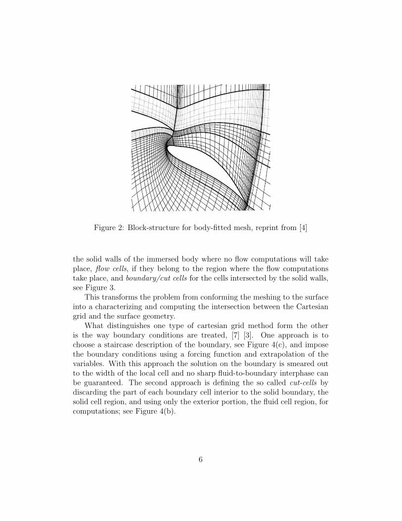
b. Complicated geometries require the use of a block-structure grid formedby several connected curvilinear regions, see Figure 2,
4
Figure 1: Mesh examples, reprint from [9]
c. The process requires user intervention, it cannot be turned into anautomatic procedure.
d. Computations based on this grids are not very robust due to secondaryfluxes through the diagonal grid faces.
e. Very sensitive to CAD geometry, requires clean representation of thesurfaces.
f. Requires the transformation of the governing equations to curvilinearcoordinates resulting in complex systems of equations which adverselyimpacts the stability, convergence, and number of operations for thesolution.
1.2 Cartesian grid
Cartesian grid methods differ from body-fitted methods in that they are non-body fitted. The whole domain is divided by a hexahedral grid system, a setof right parallelepipeds, extending through solid walls within the computa-tional domain. The cells are then flagged as solid cells, if they belong inside
5
Figure 2: Block-structure for body-fitted mesh, reprint from [4]
the solid walls of the immersed body where no flow computations will takeplace, flow cells, if they belong to the region where the flow computationstake place, and boundary/cut cells for the cells intersected by the solid walls,see Figure 3.
This transforms the problem from conforming the meshing to the surfaceinto a characterizing and computing the intersection between the Cartesiangrid and the surface geometry.
What distinguishes one type of cartesian grid method form the otheris the way boundary conditions are treated, [7] [3]. One approach is tochoose a staircase description of the boundary, see Figure 4(c), and imposethe boundary conditions using a forcing function and extrapolation of thevariables. With this approach the solution on the boundary is smeared outto the width of the local cell and no sharp fluid-to-boundary interphase canbe guaranteed. The second approach is defining the so called cut-cells bydiscarding the part of each boundary cell interior to the solid boundary, thesolid cell region, and using only the exterior portion, the fluid cell region, forcomputations; see Figure 4(b).
6
a)
b)
Figure 3: (a) Cell flagging; reprint from [1]; (b) Cell classification: flow cell,boundary cell, solid cell; reprint from [2]
Figure 4: (a) Standard scheme, (b) Cut-cell scheme; (c) Staircase implemen-tation; reprint from [8]
1.2.1 Cartesian mesh with cut cells
The remainder of this work is based on a cut-cell formulation of the boundaryconditions for a cartesian mesh where the surface of the immersed body con-sists of triangular elements obtained from a previous triangulation process.
7
In this section we briefly review the procedure for this approach and list itsadvantages and disadvantages.
As it was already mentioned, the first step in generating a Cartesian gridis performing a cell division of the domain using a uniform hexahedral grid.Once the hexahedral cells have been defined they are marked, or flagged,as solid cells, fluid cells and cut-cells. Usually the solid cells are discardedunless other calculations will take place inside the immersed body.
The cut cells are then treated by dividing them into the region intersectingthe immersed body and the region out side the body; usually the region insidethe body is discarded as well.
The geometry of the immersed boundary is analyzed for each cell andrefined based on criterions to capture the geometry of the body in a moreprecise manner.
Boundary-cells are intersected by the boundary in an arbitrary way whichleads to complex intersections between the surface triangulation and the cut-cells. Both Cartesian cells and the triangles are convex so their intersectionsresults in a convex polygon referred as triangle-polygon, tp. The edges of thetriangle-polygons are obtained by clipping the edges of the triangles alongthe faces of the cartesian cell resulting in the face-segments, fs. The divisionof the faces of the cartesian cell by along their intersection with the surfacetriangulation result in the face-polygons, fp. This can be seen for an arbitraryCut-cell in Figure 5
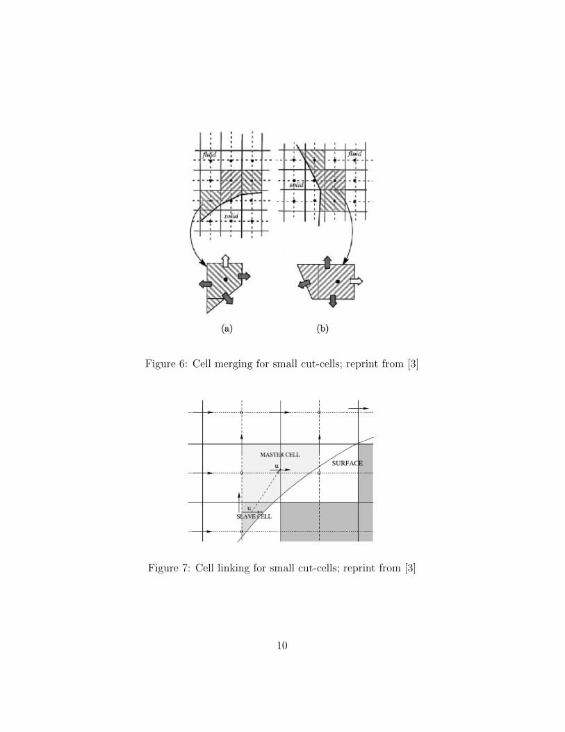
Because the surface can intersect the Cartesian mesh in an arbitrary way,the above mentioned process may produce small cut-cells which adverselyaffect the stability of the numerical method. To deal with this problemsthree procedures can be commonly found in literature,c.f. [10], [3],[6]
a. cell merging, Figure 6
b. cell linking, Figure 7
c. mixed approach
The three approaches have advantages and disadvantages and will betreated and studied if required during the development of the project. Ingeneral cell-linking does not perform very well for moving boundaries, [3].
After obtaining the cut-cells the grid may be refined if it is required. As-sessment for the need of refinement is based on the curvature of the boundary
8
Figure 5: Anatomy of a cut cell; reprint from [1]
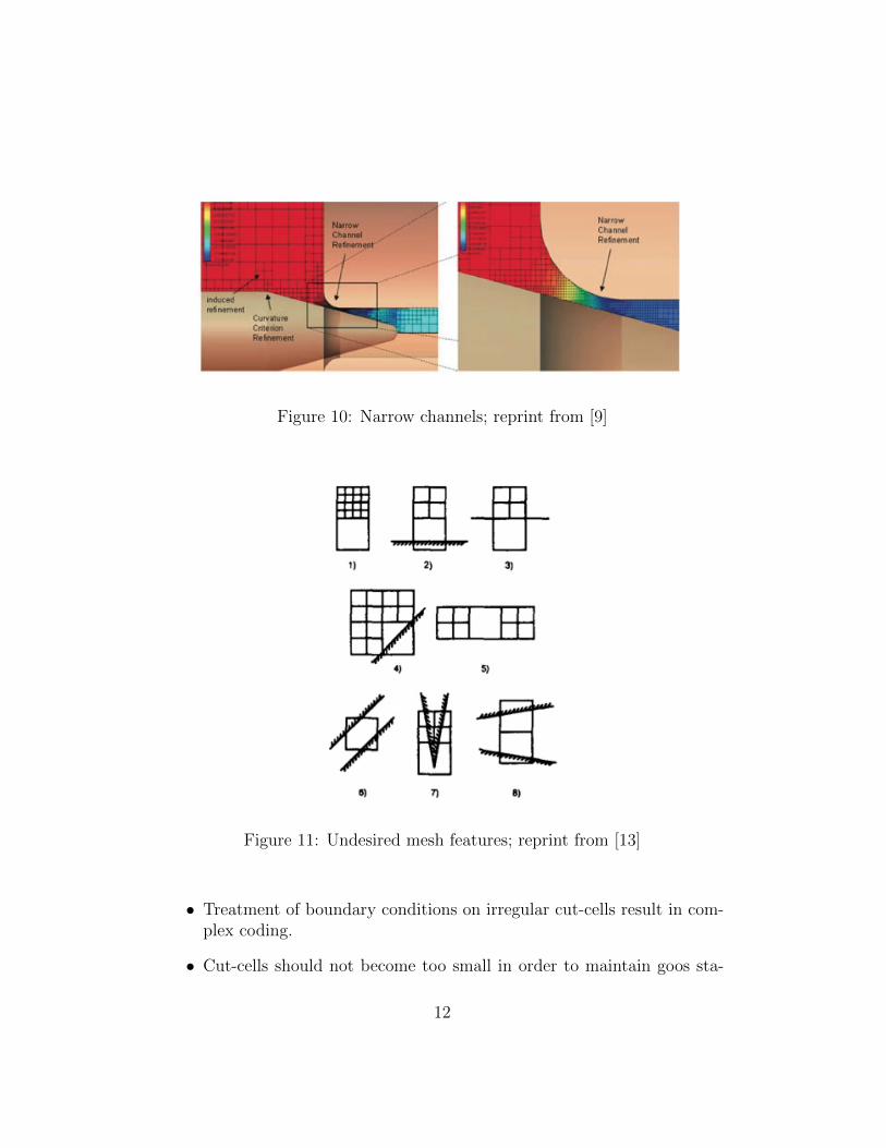
inside each cut-cell, the curvature difference between neighboring cells, Fig-ure 8, and geometrical features of the problem such as small solids and narrowchannels, Figures 9 and 10.
Refinement is based on thresholds for the acceptable curvature and thecapacity of the mesh to capture enough detail of the geometry. The refine-ment process is performed by splitting each cell into two equal cells, cellsplitting can take into account the flow direction for anisotropic refinement.Each time a cell is divided for refinement it is said that its refinement levelhas increased by one unit. The goal is to obtain a mesh not containing anyof the following features, c.f. [13], see figure(11):
• Cell refinement level differences greater than 1 between two neighboringcells.
• Cell refinement level differences greater than 0 normal to body cut-cells.
• Cell refinement level differences greater than 0 through outer flowboundaries.
• Cell refinement level differences greater than 0 between three-sided cellsand their neighbors.
9
Figure 6: Cell merging for small cut-cells; reprint from [3]
Figure 7: Cell linking for small cut-cells; reprint from [3]
10
Figure 8: Measurement for the curvature inside each cut cell and betweenneighboring cells; reprint from [1]
Figure 9: small geometrical features; reprint from [9]
• “Holes” in the mesh
• More than two cuts on a cell
• Cell refinement level differences greater than 0 on trailing edge of body.
• Bodies too close, only two cells apart.
With all the above process each Cut-cell is obtained, and thus the finalgrid.
Cartesian Meshes possess some disadvantages, c.f.[3],[1], [9]:
• Some geometrical features such as trailing edges and leading edges,require many levels of refinement
11
Figure 10: Narrow channels; reprint from [9]
Figure 11: Undesired mesh features; reprint from [13]
• Treatment of boundary conditions on irregular cut-cells result in com-plex coding.
• Cut-cells should not become too small in order to maintain goos sta-
12
bility and convergence of the solution.
• Bodies too close, only two cells apart.
But in general are well balanced by the advantages the possess, c.f.[3],[1], [9]:
• Easy to convert into an automatic procedure.
• The meshing difficulties are restricted to lower order manifolds.
• It is possible to accurately impose the boundary conditions in the cut-cells.
• Cut-cell treatment of boundaries result in conservative schemes.
• Cut-cells are decoupled from the surface description.
• Easy implementation with adaptively refined grids.
• Away from the surfaces the good quality of the grid, uniform and or-thogonal, imply better accuracy, lower discretization error and moreefficiency.
• The meshing process is not linked to a particular representation ofthe boundaries, (NURB, CAD, triangulation, etcetera). The meshingprocess may be done using “dirty geometries”, Figure 12
• Motion of the boundaries may be pre-programed and the implementa-tion for moving geometries y quite straight forward.
• Permit the use of high resolution methods.
• Good for iterative methods.
• Good for multiphase/multimaterial flows.
13
Figure 12: Schematics of dirty geometry; reprint from [9]
2 Introduction: Point-in-Polyhedron, Point-
in-Polygon Problem
The Point-in-Polygon Problem, PIP, is one of the most elementary problemsin computational geometry, it refers to the problem of determining wether apoint R lies inside a polygon P , [16]. The Point-in-Polyhedron Problem isthe extension to three dimensional space.
This problem arises naturally when constructing cartesian meshes due tothe need to determine the sections of the cut cells inside and outside the flow,Figure(13). Accurate determination of the inner and outer regions of eachcut-cell is important in order to preserve the conservative properties of thenumerical method.
In this section the most common solutions to this problem will be re-viewed.
14
Figure 13: Point-in-Polyhedron Problem in meshing; reprint from [11]
2.1 Definitions
A polygon P is a set of n-points p0, p1, . . . , pn in the plane, called vertices,and n-line segments e0 = p0p1, e1 = p1p2, . . . , en = pnp0 called edges, wherethe union of all edges divides the plane into two regions, one bounded andone unbounded, see Figure(14), [21].
Figure 14: Point-in-Polyhedron Problem; reprint from [22]
A polygon is called simple if it satisfies two conditions, [16]:
• neighboring line segments meet at only one point
• non-neighboring line segments do not have any point in common.
15
these conditions imply that in a simple polygon non of its edges intersect ortouch.
A vertex is called convex if less than half a small circe, centered at thevertex, is occupied by the polygon. Equivalently a polygon is convex if astraight line intersects the polygon’s boundary at most twice, [16], [15], seeFigure(15) .
Figure 15: Convex vertex a, non-convex vertex b, ; reprint from [16]
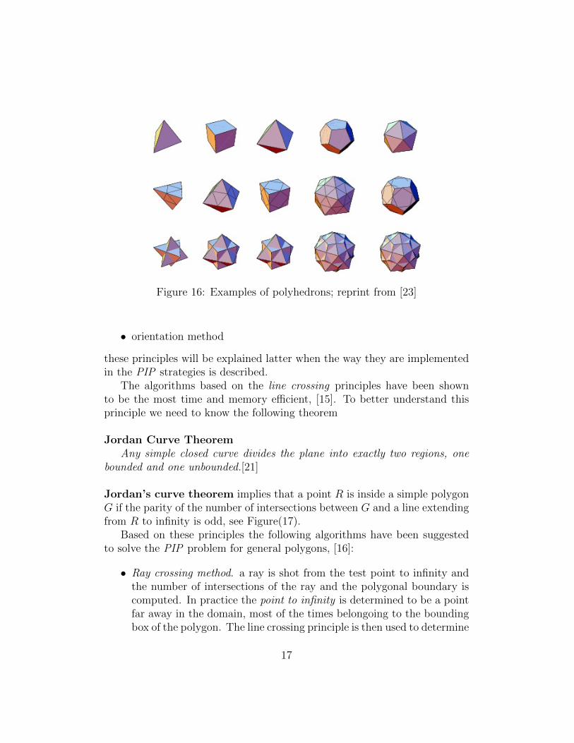
A polyhedron is a set of piecewise planar polygons that bound a solid inR3, its faces are the planar polygons, see Figure(16), [21]. This definition isvague, but it is a difficult task to define properly this class of objects properlyand it is beyond the scope of this work. A polyhedron is called simple if itsfaces do not intersect and it is called convex if any straight line intersect itsfaces at most two times, [15].
2.2 PIP algorithms
Many solution to the PIP problem can be found in the literature. Theprinciples upon which these algorithms are based are, [15]:
• line crossing
• angle-sum
• area-sum
16
Figure 16: Examples of polyhedrons; reprint from [23]
• orientation method
these principles will be explained latter when the way they are implementedin the PIP strategies is described.
The algorithms based on the line crossing principles have been shownto be the most time and memory efficient, [15]. To better understand thisprinciple we need to know the following theorem
Jordan Curve TheoremAny simple closed curve divides the plane into exactly two regions, one
bounded and one unbounded.[21]
Jordan’s curve theorem implies that a point R is inside a simple polygonG if the parity of the number of intersections between G and a line extendingfrom R to infinity is odd, see Figure(17).
Based on these principles the following algorithms have been suggestedto solve the PIP problem for general polygons, [16]:
• Ray crossing method. a ray is shot from the test point to infinity andthe number of intersections of the ray and the polygonal boundary iscomputed. In practice the point to infinity is determined to be a pointfar away in the domain, most of the times belongoing to the boundingbox of the polygon. The line crossing principle is then used to determine
17
Figure 17: Line crossing principle; reprint from [14]
if the point is interior or exterior to the polygon, see Figures(17),(14).Works in O(n) time and solves for any polygon.
• Sum of angles The polygon is treated as a fan of triangles emanatingfrom the test point where one of the edges of each triangle is an edge ofthe original polygon and the other two edges are the segments joiningthe test point with the edge of the polygon. The angle at the vertex ofeach triangle at the test point is summed and if it is equal to 360 thetest point is determined to be inside, see Figure(18). Works in O(n)time and solves for any polygon but is sensitive to the problems of finitearithmetic, see also [1] p.60.
• Swath method This method requires pre-processing. The Polygon isfirstly divided into swaths (trapezoids) in time O(n log n). The swathwhere the point is located is determined and the Ray crossing test isapplied, see Figure(19)
• Grid method A look up grid is placed over the polygon, each of the gridcells’ is categorized as either internal, external or boundary using theline crossing principle.
• Triangle-based method The polygon is decomposed into a set of trian-gles in linear time. Each triangle is defined by a fixed vertex arbitrarilydetermined to be the origin, whereas the other two vertices are de-termined by a polygon edge. The triangles obtained are classified as
18
positively of negatively oriented. A line starting at the origin and con-taining the test point is matched with all triangles. The test point isdetermined to be interior or exterior based on the intersections of thisline with the positive and negative triangles, see Figure(20)
Other methods are mentioned in the literature but they work only forconvex polygons and will not be treated in this work.
Figure 18: Sum of angles test; reprint from [14]
Due to the nature of the Cartesin Meshing process it is natural to havea deeper look into the Grid Method as a first option to determine the innerand outer regions, relative to the flow, of the object immersed in the flow.
The Cartesian mesh can be used as the look up grid where the line cross-ing criterion is applied, see Figure(21).
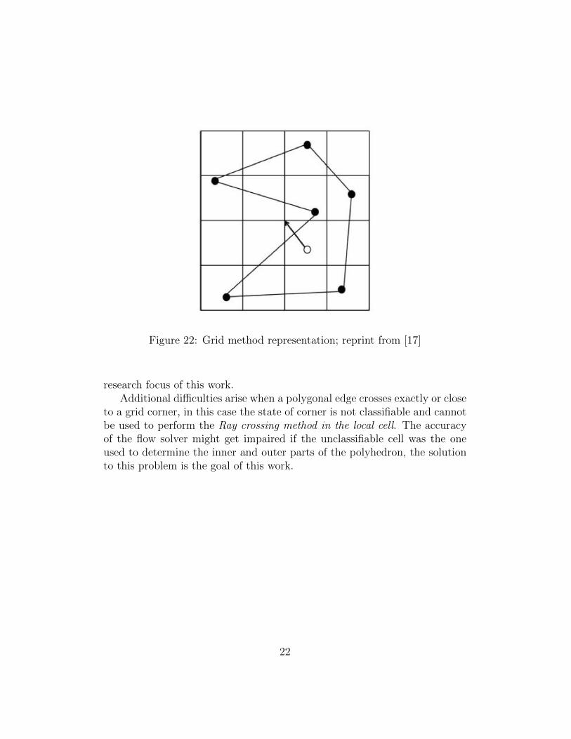
In the Grid Method the boundary cells must contain a list of edges of thepolygon that overlap their boundaries. In the cell one corner or more aredetermined to be either inside or outside the polygon. A line segment is thentraced between the test point and the corner of the cell for which the state isknown, and the state of the test point is obtained applying the line crossingprinciple, see Figure(22)
Singular conditions can occur when applying the Ray crossing method,and any other of the other method which apply the ray crossing principle.This singular conditions happen when one or more vertices of the polygonlie on the test line or when an edge of the polygon is co-linear with the test
19
Figure 19: Swath method; reprint from [19]
line. The correctness of the Grid Method can be impaired by the singularconditions which also affect the Ray crossing method,
Usually for computational geometry a uniform grid is placed as a lookup grid, but refinement can be used to obtain better accuracy and to treatsingularities.
When refinement is used it is performed in each cell until one of thefollowing occur, [17]:
• There are no more edges of the polygonal interface inside the cell.
• There is at most one vertex of the polygonal interface inside the cellwith at most two edges of the polygonal interface crossing the bound-aries of the cell.
20
Figure 20: Triangle-based method; reprint from [14]
Figure 21: Example of refined Cartesian mesh used as look up grid; reprintfrom [17]
• There are no vertex of the polygonal interface inside the cell and thereis at most one edge of the polygonal interface crossing the boundaries.
Refinement criterions for the look up grid might not be compatible withthe refinement criterions for the Cartesian Mesh, this will be part of the
21
Figure 22: Grid method representation; reprint from [17]
research focus of this work.Additional difficulties arise when a polygonal edge crosses exactly or close
to a grid corner, in this case the state of corner is not classifiable and cannotbe used to perform the Ray crossing method in the local cell. The accuracyof the flow solver might get impaired if the unclassifiable cell was the oneused to determine the inner and outer parts of the polyhedron, the solutionto this problem is the goal of this work.
22
3 Tracking the Propagating interface: Level
set method
Once the numerical methods to solve the flow and the mechanics of the airbaghave been defined, a way to obtain the evolution of the moving interface,airbag, needs to be developed. Accurate tracking of the interface is essentialto keep the conservative properties of the Finite Volume solver.
In this section a review of the Level-set method is reviewed. This approachto the airbag deployment tracking has been shown in [5] to be both efficientand robust. The advantage of this method is that the inside and outsideof the moving interface can be determined by the use of a signed distancefunction, which avoids the Point-in-polyhedron problem.
3.1 Level Set Method: Despription
The Level Set Method is a technique to track the movement of an interfaceand shapes when the velocity for each point of the interface is known. TheLevel Set approach allows to perform computations involving curves and sur-faces on a fixed Cartesian grid without having to parametrize the objects.This makes it suitable to study the evolution of objects that change in topol-ogy, that is, when the interface splits or merges as well as when holes formin it.
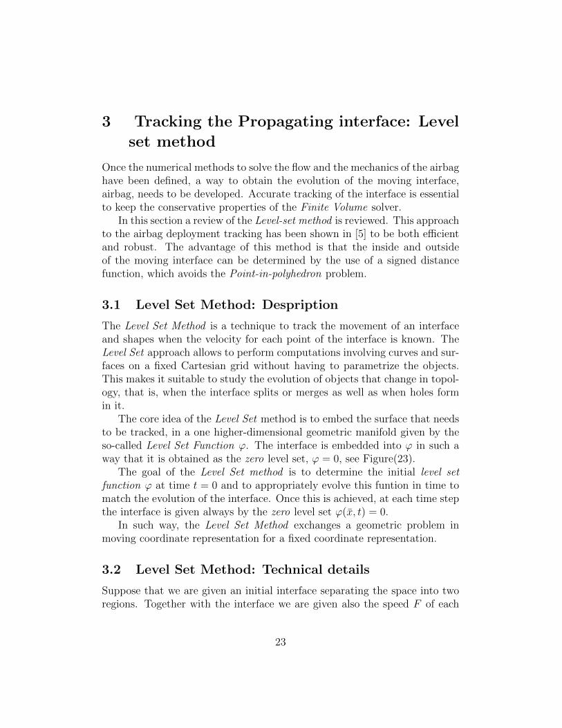
The core idea of the Level Set method is to embed the surface that needsto be tracked, in a one higher-dimensional geometric manifold given by theso-called Level Set Function ϕ. The interface is embedded into ϕ in such away that it is obtained as the zero level set, ϕ = 0, see Figure(23).
The goal of the Level Set method is to determine the initial level setfunction ϕ at time t = 0 and to appropriately evolve this funtion in time tomatch the evolution of the interface. Once this is achieved, at each time stepthe interface is given always by the zero level set ϕ(x, t) = 0.
In such way, the Level Set Method exchanges a geometric problem inmoving coordinate representation for a fixed coordinate representation.
3.2 Level Set Method: Technical details
Suppose that we are given an initial interface separating the space into tworegions. Together with the interface we are given also the speed F of each
23
Figure 23: Representation of Level Set method; reprint from [24]
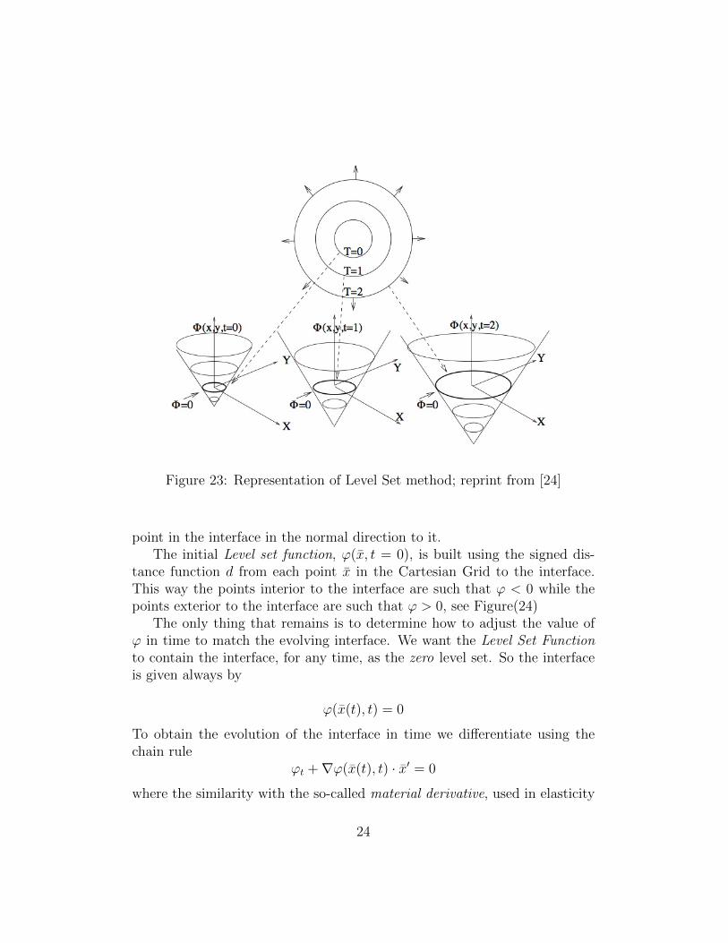
point in the interface in the normal direction to it.The initial Level set function, ϕ(x, t = 0), is built using the signed dis-
tance function d from each point x in the Cartesian Grid to the interface.This way the points interior to the interface are such that ϕ < 0 while thepoints exterior to the interface are such that ϕ > 0, see Figure(24)
The only thing that remains is to determine how to adjust the value ofϕ in time to match the evolving interface. We want the Level Set Functionto contain the interface, for any time, as the zero level set. So the interfaceis given always by
ϕ(x(t), t) = 0
To obtain the evolution of the interface in time we differentiate using thechain rule
ϕt +∇ϕ(x(t), t) · x′ = 0
where the similarity with the so-called material derivative, used in elasticity
24
Figure 24: Decomposition of space into interior and exterior according tosign of ϕ; reprint from [26]
and fluid mechanics to describe the temporal change of a property due toboth its change in position and time.
Only the normal speed F = x′ · n to the interface results in variations onits shape, so the last equation can be written as
ϕt + F |∇ϕ| = 0 (1)
where we used n = ∇ϕ/|∇ϕ|. Equation(1) is know as the level set equation.Thus, an initial value problem is obtained.
ϕt + F |∇ϕ| = 0
Γ(t) = (x, y)|ϕ(x, t) = 0
Stated as it is, and thinking of the solution in purely geometric terms,problems with uniqueness of the solution are encountered. The purely geo-metric approach to the solution is to move all the points with speed F in the
25
direction normal to the initial front. A second approach is to think of thefront moving as if it were a wave front moving. The solution is given by theenvelope of the waves emanating form each point, which satisfies uniquenessrequirements. Both approaches are represented in Figure(25).
Figure 25: Moving interface. a) moving each point normal to the curve; b)using the envelope of the wave fronts emanating from each point; reprintfrom [24]
It can be shown that the solution obtained from the envelope of the wavefront envelope is the same as the solution of the associate viscous problemϕt + F |∇ϕ| = ε∇2ϕ in the limit as ε→ 0, see Figure(26)
Figure 26: Solution to viscous problem; reprint from [24]
26
3.3 Level Set Method: Advantages and Disadvantages
For the interface tracking problem, the Level Set Method possesses certainadvantages over other approaches, [26], [24], [25]:
• The general procedure is unchanged for any number of dimensions.
• Topological changes in the front are handled naturally.
• Rely on the viscosity solution of the associate partial differential equa-tion.
• Can be converted into a computational scheme by using the alreadyknown schemes from hyperbolic conservation laws.
• There exist computational strategies to make it a more efficient proce-dure.
The only point of precaution when turning it into a computational schemeis the dependence on the CFL condition.
3.4 Level Set Method: Application to airbag deploy-ment
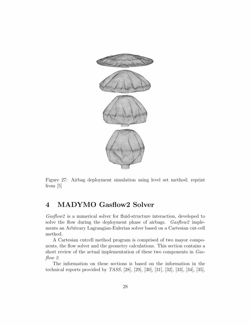
The Level Set Method can be applied as a coupling algorithm for Eulerian-Lagrangian shell-fluid interaction as shown in [5] and [27], see Figure(27).
The arbitrary boundary of the airbag is immersed in the Cartesian Meshcreating cut-cells. By filling this cut-cells and a small layer of neighboringregular cells with an appropriate ghost fluid, cell updates is performed in thesame way as the bulk cells in the computational domain. The discontinuitiesin the flow field resulting form the interface are directly embedded in thesolution through appropriately populated ghost cells, [5], [27]. This approachis known as the ghost fluid method.
At each time step the signed distance from the deformed shell to the gridpoints in the Cartesian Mesh is computed resulting in an implicit represen-tation of the fluid-shell boundary.
Because this approach avoids the generation of small cells, derived formthe conformity requirement of the mesh at the interface and thus the useof cut cells, it has also the advantage of having less restrictive time stepconstrains.
27
Figure 27: Airbag deployment simulation using level set method; reprintfrom [5]
4 MADYMO Gasflow2 Solver
Gasflow2 is a numerical solver for fluid-structure interaction, developed tosolve the flow during the deployment phase of airbags. Gasflow2 imple-ments an Arbitrary Lagrangian-Eulerian solver based on a Cartesian cut-cellmethod.
A Cartesian cutcell method program is comprised of two mayor compo-nents, the flow solver and the geometry calculations. This section contains ashort review of the actual implementation of these two components in Gas-flow 2.
The information on these sections is based on the information in thetechnical reports provided by TASS, [28], [29], [30], [31], [32], [33], [34], [35],
28
[36], [37]
4.1 Flow solver in Gasflow2
Gasflow2 approximates the flow solution based on Euler’s equations in 3-dimensional space. The flow is assumed to be a single component caloricallyperfect gas, i.e. the specific heat for both constant pressure and volume,denoted by cp and cv, are assumed to be constant.
For a bounded region Ω in R3, with boundary S, Euler’s equations read
d
dt
∫Ω
qdΩ +
∫S
Φ(q, n)dS = S(q) (2)
where
q =
ρρuρvρwρe
, and Φ =
ρvn
ρvnu+ p · nxρvnv + p · nyρvnw + p · nz
ρvnH
(3)
where n = (nx, ny, nz) is the outward normal of S, v = (u, v, w) is the velocityCartesian vector and S(q) denotes a general source term.
The total energy per unit volume is ρe = ρuint + 12ρ(v ·v) but during the
simulation it is computed from p = ((cp/cv)− 1)(ρe− 1
2ρ(v · v)
).
A correction needs to be done at the interface with the airbag due to themovement of it produced by the flow. To apply the interface conditions anArbitrary Lagrangian-Eulerian (ALE) formulation is used.
The airbag edge is described though a set of triangular segments whoseposition is approximated using a Finite Element solver.
For the fluid-structure interface the the two interface conditions thatneeds to be satisfied are the kinematic condition
vf = vs
and the dynamic conditionσf = σs
where σ is the stress tensor σ = pI + τ .For an inviscid fluid the structure-fluid coupling, with structure velocity
vs and flow velocity vf , conditions result in
vf · n = vs · n and pf = ps (4)
29
In the ALE formulation Euler equation’s for the fluid domain are givenby
d
dt
∫Ω(t)
qdΩ +
∫S(t)
Φ(q,vs) · ndS = S(q) (5)
where the flux function through the control volume boundary and the bound-ary state vectors are defined as
The discretization of the Euler equations is performed through the Methodof Lines. The spatial derivatives are replaced by algebraic approximations,using Finite Volumes approach, to obtain a system of Ordinary DifferentialEquations where only time remains as a variable. The next step is to applyan integration algorithm for initial value Ordinary Differential Equations tocompute the approximate solution of the original Partial Differentia Equa-tion. In other words, the Method of Lines discretizes the spatial and temporalderivatives separately.
The spatial discretization is performed by a Finite Volumes method overhexahedral cells. The finite Volumes used in Gasflow2 is based on a Roescheme where the flux derivatives are approximated using a flow-differencingsplitting scheme. This formulation does not allow discontinuous expansionfans.
To obtain a second order space discretization, the state of the cell face iscomputed from the state at the cell center assuming a linear variation of theform
qk(x) = qk(xc) + (Ψk(∇qk))T · (x− xc).
30
The gradient reconstruction for a component qk in cell Ωj follows formthe minimization of the functional
J =1
2
∑j∈N
||∇qk ·∆xj −∆qj||2
where N is the set of all faces of cell m and j is the index of the face whichseparates cell m and the neighbor n. Here ∆xj = xm − xn is the distancebetween the cell centers and ∆qj = qm−qn. This leads to a non-square linearproblem which is equivalent to the solution of the system of normal equation.The system of normal equations is SPD and can be solved by direct methods.
The task of the limiter Ψ is to enforce the monotonicity principle, whichrequires that the reconstructed values does not exceed teh maximum andminimum of the neighboring centroid values and its own cell center value.The limiter acts in each component of q. For a uniform mesh with cubic cellsof length h, where Ψ = 1 the reconstruction has truncation error O(h2) andin regions where Ψ = 0 the reconstruction has truncation error O(h1).
The two limiters implemented are the Venkatakrishnan-limiter and theBarth-Jespersen limiter. Both are applied through directional limiting.
The temporal integration is performed via a Runge-Kutta method. Thevolumes are not assumed to be constant so the Runge-Kutta as applied inthe discretization is also valid for changing cells, as is the case with AdaptiveMesh Refinement.
In general for a Cartesian Mesh without cutcells the time step restrictionfor the Runge-Kutta method follows from
τ = minj∈Nc , with τj =σ∆j
λmax
where Nc is the set of cells, ∆j is the cell size of cell j, σ is the Courantnumber, and λmax is the maximum wave speed of the system, [31].
As mentioned before, the volume of the cut-cells can be smaller than thesmallest Cartesian cell which leads to stability problems. To avoid stabilityproblems, cut-cells whose volume is smaller than that of the smallest Carte-sian cells, are merged into clusters used to update the state vectors in thenext time step. The stability criterion for the time step for the clustered cellsfollows from
∆t = minj∈Nc
|Ω|minσ∑Nf
k=1 Ψk
31
where Ψk = (a + vn)kSk. The merging partner is selected based on thedirection most normal to the boundary face.
4.1.2 Boundary conditions
In order to have a well posed problem, initial conditions and boundary con-ditions must be specified.
Initial conditions should satisfy (2) inside the domain and the boundaryconditions should specify the state vector completely and conditions (4) haveto be satisfied in the boundary and implemented on the discretization.
Boundary conditions for the cells are enforced through the specificationof the fluxes at the boundary. For each cell face there are seven possibleconditions
• wall
• subsonic inflow
• sonic inflow
• supersonic inflow
• subsonic outflow
• sonic outflow
• supersonic outflow
The specification of each of these boundary conditions depends on theeigenvalues of the flux Jacobi matrix Φ.
For the non-stationary boundary created by the airbag the velocity of theflow prescribes the normal velocity component of the airbag
vn = Vn
and the boundary flux density ΦB is computed using the relative velocities
Conditions (4) are implemented through the definitions of the fluxes inΦ as defined in (6). The structural velocity at each cell center xc is obtainedthrough means of interpolation between the Finite Element nodes accordingto
vs(xc) =3∑i=1
Ni(ξ)vN,i
where vN,i is the nodal velocity and Ni(ξ) is the local shape function evalu-ated in the FE-segment transformed coordinate system.
The pressure in the cutcells contributes to each of the nodal forces ofthe FE partition inside the cutcell. The FE segments inside each cutcell arepartitioned into Nsp-number of segment polygons, which each exert a force
fp,j = pj(xc)njSj
on the FE segment. The total contribution to node i is computed accordingto
fN,i =
Nsp∑j=1
Ni(ξ)fp,j.
The coupling is obtained by a standard loose-coupling procedure, i.e., ateach time step one evaluation of FE and flow solver are performed.
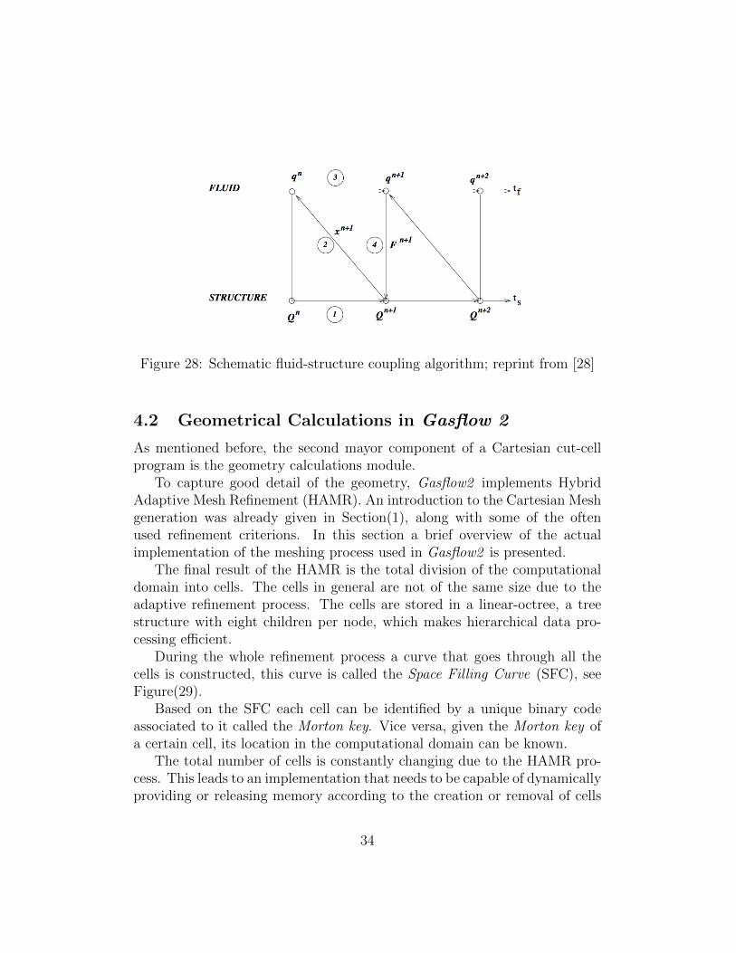
For known locations of the FE elements, the fluid solution is advancedover one time step returning new contributions to the nodal forces fn to theFE solver. The coupling procedure is represented in Figure(28)
33
Figure 28: Schematic fluid-structure coupling algorithm; reprint from [28]
4.2 Geometrical Calculations in Gasflow 2
As mentioned before, the second mayor component of a Cartesian cut-cellprogram is the geometry calculations module.
To capture good detail of the geometry, Gasflow2 implements HybridAdaptive Mesh Refinement (HAMR). An introduction to the Cartesian Meshgeneration was already given in Section(1), along with some of the oftenused refinement criterions. In this section a brief overview of the actualimplementation of the meshing process used in Gasflow2 is presented.
The final result of the HAMR is the total division of the computationaldomain into cells. The cells in general are not of the same size due to theadaptive refinement process. The cells are stored in a linear-octree, a treestructure with eight children per node, which makes hierarchical data pro-cessing efficient.
During the whole refinement process a curve that goes through all thecells is constructed, this curve is called the Space Filling Curve (SFC), seeFigure(29).
Based on the SFC each cell can be identified by a unique binary codeassociated to it called the Morton key. Vice versa, given the Morton key ofa certain cell, its location in the computational domain can be known.
The total number of cells is constantly changing due to the HAMR pro-cess. This leads to an implementation that needs to be capable of dynamicallyproviding or releasing memory according to the creation or removal of cells
34
Figure 29: Space Filling Curve; reprint from [37]
during the process.To satisfy such memory needs the whole octree structure of the cells is
stored as a linked list forming a linear-octree. The one dimensional list of cellsfollows the order of the SFC, see Figure(30) for a bi-dimensional example.
Figure 30: Space Filling Curve and octree representation; reprint from [37]
Sets of new cells can be added or removed at arbitrarily positions to thelinked list to allow for dynamic memory management.
As it can be seen from Figure(30), the whole domain can be divided intosubdomains, following the order of the SFC, containing the same numberof cells, these subdomains are called blocks. The purpose of the block is to
35
define regions with equal distribution of computation workloads which canbe later used for parallel computing and to treat regions of the whole domainseparately according to their refinement needs. To manage efficient computa-tion, each block contains relevant information about the connectivity of thecells in it, and each cell contains relevant informations about its neighborsas well as access to information regarding the flow solution in its centroid,and relevant geometric information about itself.
The HAMR process is performed in two main steps. The first step ofthe HAMR is build an initial Block Frame Work (BFW) based on the initialgeometry and solution at each time step.
Building the BFW is achieved in five steps
1- Generation of a uniform mesh of empty blocks for the whole domain.Blocks are said to be empty because at this point they contain nogeometrical or flow information.
2- Use of a search algorithm to identify and tag the blocks that intersect theflow domain.
3- Create an internal cell mesh in each tagged block. At these point themesh is uniform inside all blocks.
4- Set initial flow solution in the obtained mesh.
5- Set boundary conditions for the cell faces.
The generation of the BFW is a simplified version of the whole HAMRprocess where refinement occurs only once in the tagged blocks and the finalmesh, internal to each block, is uniform in size.
Once the BFW is defined the second step of the HAMR takes place.Using a search algorithm blocks are tagged for further refinement based ontwo criterions
1- A block is tagged as a result of intersecting with at least one segment ofthe FE partition.
2- A block is tagged as a result of having a more than one refinement levelless than any of its neighboring blocks.
36
Because each cell is identified by a Morton key, the availablility width ofthe key determines the achievable resolution for refinement.
After each refinement, the second step of the HAMR process starts. Thisis performed until no further refinement can be performed based on theachievable resolution defined by the length of the Morton key.
After the refinement process is completed, the cells that intersect anysegment of the FE triangulation of the airbag are tagged by the search al-gorithm and the exact geometry of the cut-cells is computed, obtaining arepresentation of each cut-cell as shown in Figure(5)
In practice the search algorithm is performed in three stages, each withdifferent levels of accuracy. The accuracy of the stages of the search algorithmvary from finding list of possible FE segment intersecting each block, tofinding the actual FE segment intersection with each cell.
To avoid making the HAMR a too intense computational process, notall three stages of the search algorithm are performed at each time step andrefinement loop. For instance to build the initial BFW only the first level ofaccuracy of the search algorithm is used.
37
5 Cut cell construction, problem description
In this section an in-depth description of the search algorithm is presentedwith emphasis in the last stage where the exact geometry of the cut-cells isobtained.
The process to obtain the final cut-cells, as shown in Figure(5), is draftedin [29] and its implementations is presented in [34].
This section is based on the before mentioned [29] and [34], as well as incommunications with Ir. E.H. Tazammourti.
The purpose of the search algorithm is to classify the cells into, activecells, inactive cells and cut cells, as well as to build the exact geometry of thecut-cells for the FV solver. The search algorithm is divided into three stages
• Global search level. This search determines a list of candidate segmentsthat may intersect each bock, see Section(4.2) .
• Euler search. This search determines a set of segments that may inter-sect every cell.
• Exact Geometry. This search determines all intersections between Eulercells and FE-segments using the intersection candidate list. After thatthe face polygons, boundary faces and polyhedrons of each cut cell areobtained.
5.1 Global search level
The Cartesian cut-cell methodology used in MADYMO, along with the Ar-bitrary Lagragian-Eulerian formulation for the coupling between the airbaginterface and the flux, results in the use of two different meshes, the Eulermesh, used for the flow calculations and the FE-mesh, used for tracking thestructure of the airbag. The Euler mesh is formed by the hexahedral cellsthat divide the whole domain and the FE mesh is formed by the triangularsegments which represent the airbag surface.
During the solution process these two meshes share information. TheEuler mesh sends forces resulting from the flow to the FE-segments, and theFE-mesh sends geometric information to the Euler mesh to build the fluxesrequired by the FV solver.
During the Global search level, the FE-mesh uses the bounding box of theFE-segments to analyze the intersection of the bonding box with the Block
38
Frame Work (BFW), see Section(4.2), of the Euler mesh. During this stepthe bounding box of the FE-segments if defined with an off-set. As a result,the final list of segments intersecting the BFW is constituted by candidatesegments, not the final ones. The off-set is used so that this stage of thesearch algorithm does not have to be repeated at every time step, it is onlyperformed every time the displacement of the FE-segments is larger than theoff-set.
The main topological tool used at this stage is verifying the intersectionof two boxes. As a result of this Global search a list of possible segmentsintersecting each block is creates and stored in a list called sblock. For eachblock on the Euler mesh an sblock is created. Each block receives its ownsblock to perform the next level of search. The process is represented inFigure(31a)
Figure 31: global search level
39
At the end of the global search each block which intersects the flow region,active block, is tagged and each block receives a list of possible segmentsintersecting it, which is called sblock
5.2 Euler search level
The Euler search level is performed in the same way as the Global search butat block level.
For each block in the Euler mesh, the bounding box of each segment inits corresponding list sblock is verified for intersection with each one of thecells in the block.
To reduce computational cost, this search level is performed using anoff set in the bounding box of the segments. This result in a list calledcblock of possible segments intersecting each cell in the block. The processis represented in Figure(31b).
At the end of the Euler search, each cell contains a list cblock of possiblesegments that might intersect it. At this stage the active blocks and cut-block are known as well as the active cells and cut-cells. For the cells alsothe totally immersed boundary faces are known, but the cell faces neighboringcut-cells still need to be classified. The cblock for each cut-cell contains thenecessary information to perform the Exact Geometry search level.
5.3 Exact Geometry
As a result of the the two previous levels of search, each cut-cell has a list,cblock, containing a set of candidate segments intersecting it. The purposeof the Exact Geometry search level is to detect if a certain segment of the listof candidates really intersect the cell and, if so, to calculate the intersectionpoints to construct the geometry of the cut-cell.
To test wether a certain segment intersects a cell, it is quite straightforward to think of a verification process in terms of geometry. For example,to calculate the intersection point of a certain segment’s edge with one ofthe cell’s faces one can think of solving the system for the intersection of theplane containing the cell’s face and the line containing the segment’s edge.These geometrical analysis also builds the intersection point in the process.The problem with geometrical methods is that they require the constructionof “new geometry”, called constructors, which have different precision than
40
the given data, and are subject to round off errors which at the end result inan unknown accuracy for the intersection points. [1].
Considering the problems that arise from solving the intersection problemin terms of geometrical descriptions, it is desired to first build topologicaltools to verify the actual occurrence of an intersection and if such intersectionreally happens then to build the intersection point using geometrical tools.This way the use of intersection constructors is kept to a minimum and sotheir effect on accuracy and use of computational resources. After all theintersection problem is a question of topology, not of geometry.
To achieve this, three topological tests are used
• Point test. For each FE node find in which cell it resides, see Figure(32a).
• Edge test. For each FE edge test wether it intersected by a certaincell’s face, see Figure(32b).
• Slice test. For each FE segment test wether it is intersected by a certaincell’s edge, see Figure(32c).
Figure 32: Exact Tests
In order to understand how these tests work, the concept of the signedvolume for a tetrahedron needs to be known.
41
5.3.1 Signed Volume of a Simplex
A simplex is the generalization of a triangle to n-dimensions. The simplexin 3 dimensions is the tetrahedron.
A known property for the simplex is the computation of its volume indeterminant form. This property states that the volume V (T ) of the simplexT with vertices (v0, v1, . . . vd) in d-dimensions is:
This volume is positive if the triangle ∆a,b,c forms a counterclockwisecircuit when viewed form a point located on the side of the plane defined by∆a,b,c which is opposite from d, c.f [1], see Figure(33)
Figure 33: Signed Volume Property
The side of the point d with respect to the plane defined by ∆a,b,c can bedetermined by the sign of the volume obtained vis the determinant. If thisvolume is zero the point d is coplanar with a, b, c.
42
Using the signed volume property, two tests can be defined, the piercetest and the Inside test
5.3.2 Pierce test
This test determines weather a line segment between two points a and bpierces trough the plane defined by a triangle ∆0,1,2.
Applying the signed volume test to the triangle ∆0,1,2 and the segment ab,see Figure(34), ab crosses the pane if and only if the signed volumes V (T012a)and V (T012b) have opposite signs
Figure 34: Pierce test, reprint form [1]
5.3.3 Inside test
Once it has been verified that the segment ab indeed pierces through theplane where the triangle ∆0,1,2 resides, what need to be determined is if thesegment pierces inside the triangle.
According to the signed volume property, piercing occurs inside the tri-angle if the the volume of the tetrahedrons connecting the end points ofsegment ab with the end points of the edges of the triangle ∆0,1,2 have all thesame sign, that is if:
[V (Ta,1,2,b) < 0 ∧ V (Ta,0,1,b) < 0 ∧ V (Ta,2,0,b) < 0]
or[V (Ta,1,2,b) > 0 ∧ V (Ta,0,1,b) > 0 ∧ V (Ta,2,0,b) > 0]
see Figure(35) for a graphic representation of this test.
43
Figure 35: Pierce test, reprint form [1]
5.3.4 Topological Characteristics
To obtain the topological characteristics of a cut-cell the first step is to applythe Point tests to determine which of the candidate nodes resides inside it.
The Point test transfers the point coordinates in terms of the SPF index,using this information the cell where the edge resides can be known, seeFigure(32a).
Once it is known the cell inside which a node resides, the Edge test isapplied to determine which cell face is pierced by the edges containing suchnode as an end point.
For each of the edges containing the node and for each of the cell’s faces,the Edge Test is performed in two stages. First the pierce test is used todetermine which of the cell face’s planes the edge pierces, see Figure(36a).Second, the ( inside test) is performed to determine if the segment piercesthe plane inside the cell’s face, see Figure(36b).
The last thing that needs to be determined is which of the triangularsegments of the FE-mesh cut each of the Euler cell’s edges. This is determinedusing the Slice test.
The Slice test is performed in two stages. First the pierce test is performedto determine if a certain Euler cell’s edge pierces trough any of the segment’splanes, see Figure(37a). Second, the inside test is performed to determine ifthe cell’s edge pierces inside the segment, see Figure(37b).
Degenerate cases There exist six cases where the Point test, Pierce Testor Slice test may fail, [29]
44
Figure 36: Edge test,
Figure 37: Slice test,
1- FE-node coincides with a face, see Figure(38a).
2- FE-node coincides with a cell edge, see Figure(38b).
45
3- FE-node coincides with cell vertex, see Figure(38c).
4- FE-edge intersects with a cell edge, see Figure(38d).
5- FE-edge intersects with a cell vertex, see Figure(38e).
6- FE-segment intersects with a cell vertex, see Figure(38f).
Figure 38: Degenerate cases
The first three degenerate cases cause trouble with the point test. Thetest is unable to determine the cell to which the problematic point belongs.To solve this problem a Tie breaking algorithm can be used, [1], [29].
Additionally, when cases 1, 2 or 3 occur the Edge test concludes no in-tersection because one of the signed volumes is zero. When cases 2 and 3are found also the Slice test fails because one of its components gives a zerovolume.
When cases 4 and 5 occur the Edge test fails because one of the compo-nents of the Inside test has a zero volume.
When case 6 occurs the Edge test fails because one of the components ofthe pierce test has zero volume, [29].
46
5.3.5 Geometrical Characteristics
After applying the above mentioned tests, for each cell face the FE-edgesintersecting it are known, as well as the FE-segments cutting each of thecells’ edges. The points where an FE-edge pierces a cell’s face and the pointswhere a cell’s edge intersects a segments are known as pierce points. To buildthe exact geometry of the cut-cells the pierce points need to calculated.
Geometrical constructors were originally rejected because the problem ofwether or not an edge pierces a plane inside a certain region is a problem oftopology and not of geometry. Once the existence of pierce points have beenestablished geometrical constructors should be used to generate the actualgeometry of the pierce pierce points, [1].
47
6 Problem definition and research questions
As a result of the search algorithm, described in detail in the last section, allblocks of the Euler-mesh are classified as active, if they belong completelyto the flow region, inactive if they are outside the flow region, or cut-block ifthe interface of the airbag intersects any of the cells belonging to the block.
In the same way, each cell is classified as active, inactive or cut-cell. Thecell faces are also classified, the cell faces connecting two active cells areclassified as flow faces. The faces connecting an active cell and a cut cellare classified as cut faces but this classification takes place when the cut-cell’s exact geometry is obtained. As a result of the unresolved geometricdegeneracies the faces connecting active cells to cut-cells can not be classifiedentirely.
In the actual cut-cells implementation used in MADYMO two issues needto be addressed
1- How to solve the degenerate cases? The aim of this question isto define an algorithm capable of determining consistently the existence of apierce point for the degenerate geometries.
2- How to determine which region in a cut-cell belongs to theflow and which out-side? The only known fact about the cut-cells, ingeneral, is their classification as such, but not which regions in them belongto the flow and which outside.
Thinking of a test to define the inner and outer regions of a cut-cellseems easy in terms of any of the already mentioned tests for the Point inPolyhedron Problem. For example the line crossing test could be used takingany test point in any of the two regions of a cut-cell and the centroid ofany of the active cells, tracing a line segment between those two points andcounting the number of intersections would reveal the answer. But soonproblems arise, for example:
• How to chose the test point in the cut-cell?
• How does the choice of the active cell affects the accuracy and whatrole does connectivity plays?
• What happen if the test point in the cut-cell is too close to the airbag’sboundary?
This problems become more complicated taking into account the fact thatthe boundary in the problem at hand is a moving, flexible boundary.
48
The two above mentioned questions and the derived subquestions are theresearch topic that this work will address.
49
7 Looking for solutions
In this section a description of various methods to solve the problem is pre-sented. In the first part a brief explanation on the actual solution methodimplemented in MADYMO is presented along with an example of a degen-erate geometry for which it fails.
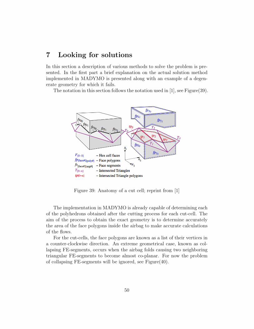
The notation in this section follows the notation used in [1], see Figure(39).
Figure 39: Anatomy of a cut cell; reprint from [1]
The implementation in MADYMO is already capable of determining eachof the polyhedrons obtained after the cutting process for each cut-cell. Theaim of the process to obtain the exact geometry is to determine accuratelythe area of the face polygons inside the airbag to make accurate calculationsof the flows.
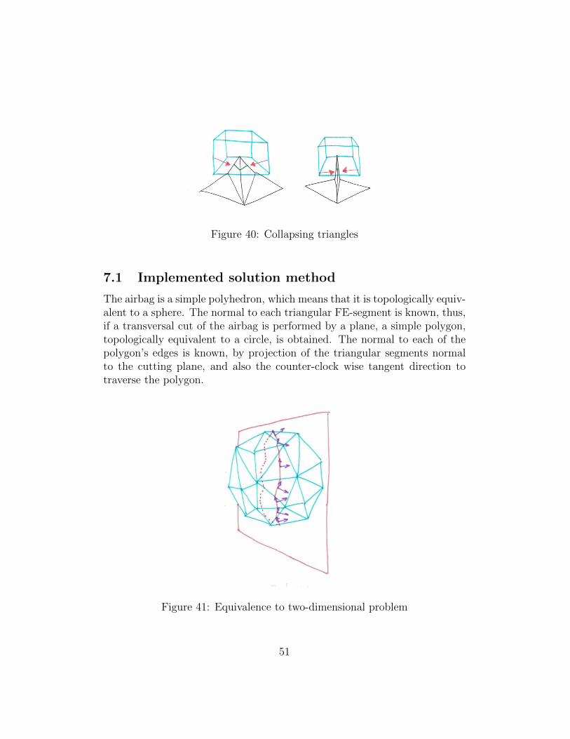
For the cut-cells, the face polygons are known as a list of their vertices ina counter-clockwise direction. An extreme geometrical case, known as col-lapsing FE-segments, occurs when the airbag folds causing two neighboringtriangular FE-segments to become almost co-planar. For now the problemof collapsing FE-segments will be ignored, see Figure(40).
50
Figure 40: Collapsing triangles
7.1 Implemented solution method
The airbag is a simple polyhedron, which means that it is topologically equiv-alent to a sphere. The normal to each triangular FE-segment is known, thus,if a transversal cut of the airbag is performed by a plane, a simple polygon,topologically equivalent to a circle, is obtained. The normal to each of thepolygon’s edges is known, by projection of the triangular segments normalto the cutting plane, and also the counter-clock wise tangent direction totraverse the polygon.
Figure 41: Equivalence to two-dimensional problem
51
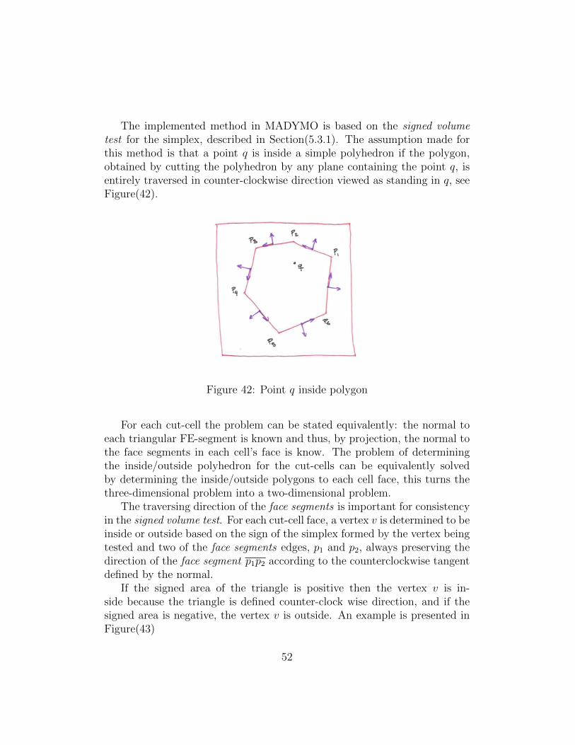
The implemented method in MADYMO is based on the signed volumetest for the simplex, described in Section(5.3.1). The assumption made forthis method is that a point q is inside a simple polyhedron if the polygon,obtained by cutting the polyhedron by any plane containing the point q, isentirely traversed in counter-clockwise direction viewed as standing in q, seeFigure(42).
Figure 42: Point q inside polygon
For each cut-cell the problem can be stated equivalently: the normal toeach triangular FE-segment is known and thus, by projection, the normal tothe face segments in each cell’s face is know. The problem of determiningthe inside/outside polyhedron for the cut-cells can be equivalently solvedby determining the inside/outside polygons to each cell face, this turns thethree-dimensional problem into a two-dimensional problem.
The traversing direction of the face segments is important for consistencyin the signed volume test. For each cut-cell face, a vertex v is determined to beinside or outside based on the sign of the simplex formed by the vertex beingtested and two of the face segments edges, p1 and p2, always preserving thedirection of the face segment p1p2 according to the counterclockwise tangentdefined by the normal.
If the signed area of the triangle is positive then the vertex v is in-side because the triangle is defined counter-clock wise direction, and if thesigned area is negative, the vertex v is outside. An example is presented inFigure(43)
52
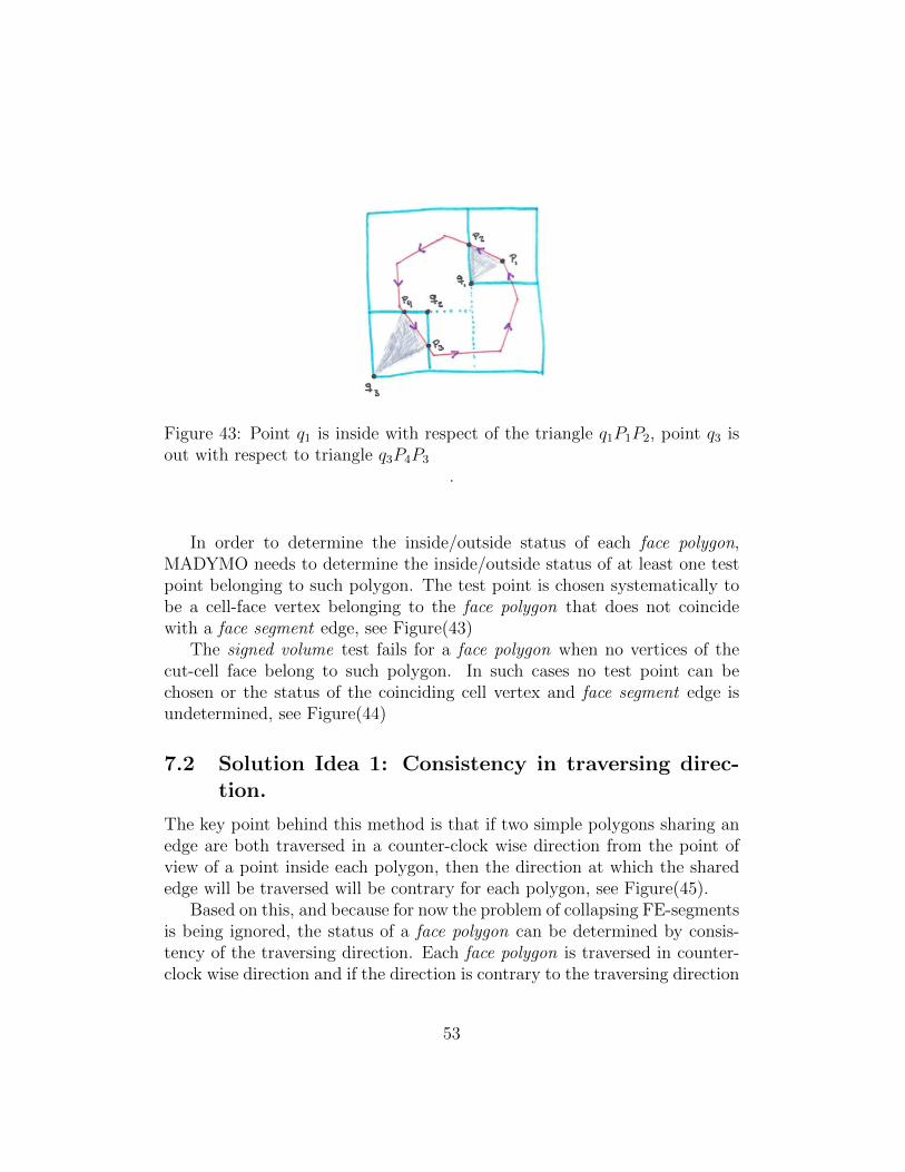
Figure 43: Point q1 is inside with respect of the triangle q1P1P2, point q3 isout with respect to triangle q3P4P3
.
In order to determine the inside/outside status of each face polygon,MADYMO needs to determine the inside/outside status of at least one testpoint belonging to such polygon. The test point is chosen systematically tobe a cell-face vertex belonging to the face polygon that does not coincidewith a face segment edge, see Figure(43)
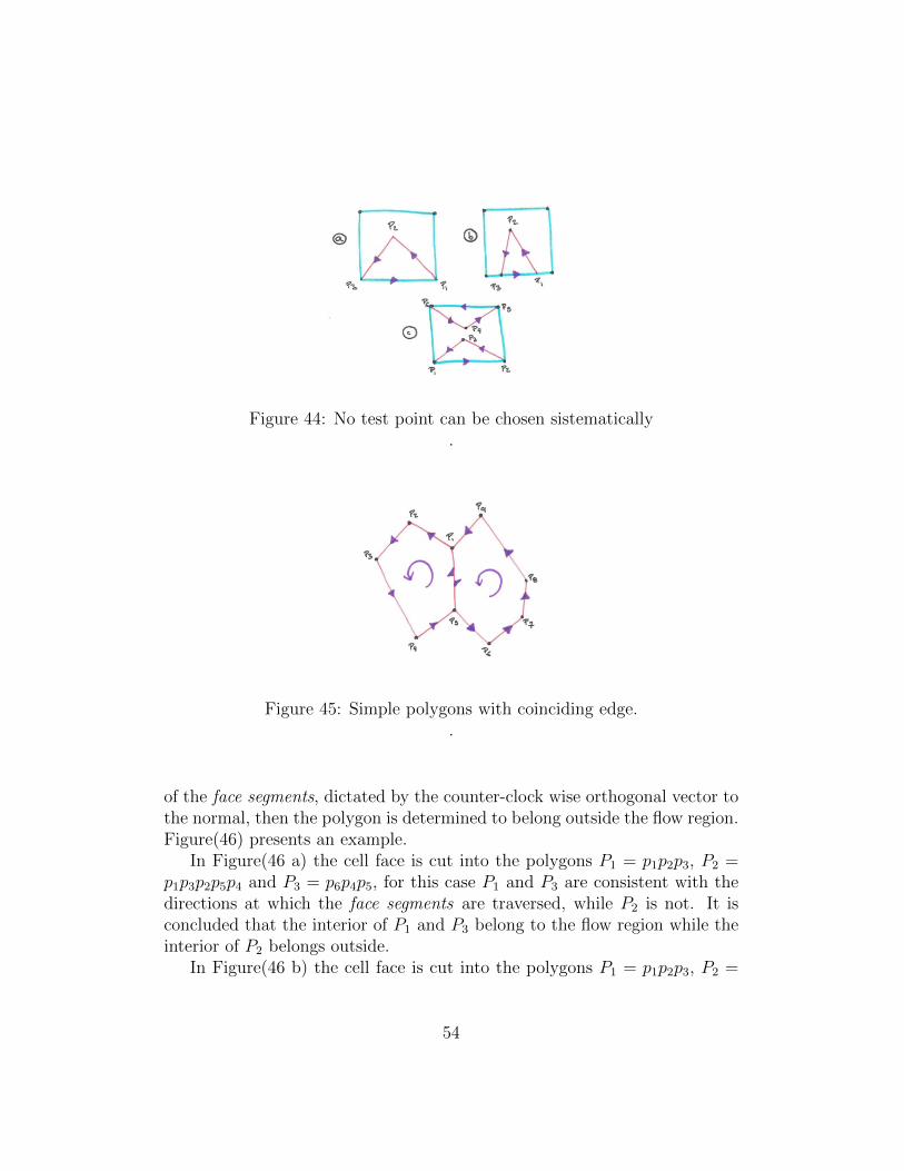
The signed volume test fails for a face polygon when no vertices of thecut-cell face belong to such polygon. In such cases no test point can bechosen or the status of the coinciding cell vertex and face segment edge isundetermined, see Figure(44)
7.2 Solution Idea 1: Consistency in traversing direc-tion.
The key point behind this method is that if two simple polygons sharing anedge are both traversed in a counter-clock wise direction from the point ofview of a point inside each polygon, then the direction at which the sharededge will be traversed will be contrary for each polygon, see Figure(45).
Based on this, and because for now the problem of collapsing FE-segmentsis being ignored, the status of a face polygon can be determined by consis-tency of the traversing direction. Each face polygon is traversed in counter-clock wise direction and if the direction is contrary to the traversing direction
53
Figure 44: No test point can be chosen sistematically.
Figure 45: Simple polygons with coinciding edge..
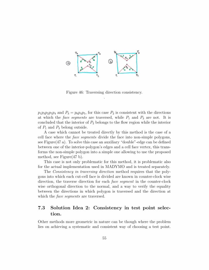
of the face segments, dictated by the counter-clock wise orthogonal vector tothe normal, then the polygon is determined to belong outside the flow region.Figure(46) presents an example.
In Figure(46 a) the cell face is cut into the polygons P1 = p1p2p3, P2 =p1p3p2p5p4 and P3 = p6p4p5, for this case P1 and P3 are consistent with thedirections at which the face segments are traversed, while P2 is not. It isconcluded that the interior of P1 and P3 belong to the flow region while theinterior of P2 belongs outside.
In Figure(46 b) the cell face is cut into the polygons P1 = p1p2p3, P2 =
54
Figure 46: Traversing direction consistency..
p1p3p2p5p4 and P3 = p6p4p5, for this case P2 is consistent with the directionsat which the face segments are traversed, while P1 and P3 are not. It isconcluded that the interior of P2 belongs to the flow region while the interiorof P1 and P3 belong outside.
A case which cannot be treated directly by this method is the case of acell face where the face segments divide the face into non-simple polygons,see Figure(47 a). To solve this case an auxiliary “double”-edge can be definedbetween one of the interior-polygon’s edges and a cell face vertex, this trans-forms the non-simple polygon into a simple one allowing to use the proposedmethod, see Figure(47 b).
This case is not only problematic for this method, it is problematic alsofor the actual implementation used in MADYMO and is treated separately.
The Consistency in traversing direction method requires that the poly-gons into which each cut-cell face is divided are known in counter-clock wisedirection, the traverse direction for each face segment in the counter-clockwise orthogonal direction to the normal, and a way to verify the equalitybetween the directions in which polygon is traversed and the direction atwhich the face segments are traversed.
7.3 Solution Idea 2: Consistency in test point selec-tion.
Other methods more geometric in nature can be though where the problemlies on achieving a systematic and consistent way of choosing a test point.
55
Figure 47: Non-simple polygon degeneracy..
Those methods will be discussed in this subsection.
References
[1] M. J. Aftosmis, Solution Adaptive Cartesian Grid Methods for Aerody-namic Flows with Complex Geometries. von Karman Institute for FluidDynamics Lecture Series 1997-02 March, 1997
[2] G. Yang, D. M. Causon, D. M. Ingram, Calculation of compressible flowsabout complex moving geometries using a three-dimensional Cartesian cutcell method. Int. J. Numer. Meth. Fluids 2000; 33: 11211151
[3] H. Bandringa, Immersed boundary method. Master Thesis in appliedmathematics, University of Groningen, August 2010
[4] L. Dubuc, F. Cantariti, M. Woodgate, B. Gribben, K. J. Badcock andB. E. Richards, A grid deformation technique for unsteady flow compu-tations. Int. J. Numer. Meth. Fluids 2000; 32: 285311
[5] F. Cirak, R. Radovitzky, A Lagrangian-Eulerian shell-fluid coupling al-gorithm based on level set methods. Computers and structures, Elesevier2005, 83
56
[6] D. Hartmann, M. Meinke, W. Schrder A strictly conservative Cartesiancut-cell method for compressible viscous flows on adaptive grids. Comput.Methods Appl. Mech. Engrg. 200 (2011) 10381052
[7] R. Mittal, G. Iccarino, Immersed boundary method. Annu. Rev. FluidMech. 2005. 37:23961
[8] S. Kang, G. Iaccarino, F. Ham, P. Moin, Prediction of wall-pressure fluc-tuation in turbulent flows with an immersed boundary method. Journal ofComputational Physics 228 (2009) 67536772
[10] M. Meyer, A. Devesa, S. Hickel, X.Y. Hu, N.A. Adams A conservativeimmersed interface method for Large-Eddy Simulation of incompressibleflows. Journal of Computational Physics, 229 (2010) 63006317
[11] J. Peteker Point-in-Polygon Detection. Bachelor Thesis University ofCalifornia, Merced, April 2010
[12] P.G. Tucker, Z. Pan, A Cartesian cut cell method for incompressibleviscous flow. Applied mathematics modeling, 24, 2000, 591-606
[13] D. De Zeeuw, K. Powell An adptive refined cartesian mesh solver forEuler equations. J. of Comp. Physics, 104, 56-69, 1993
[14] E. Haines Poin-in-Polygon strategies. Graphics Gems IV, ed. Paul Heck-bert, Academic Press, 1994, p. 24-46.
[15] D. De Zeeuw, K. Powell Efficient and consitent algorithms for deter-mining the containment of point in polygons and polyhedra. EurographicsAssociation, Elsevier Science Publications, 1987, 423-437
[16] B. Zalik, I. Kolingerova A cell-based point-in-polygon algorithm suitablefor large sets of points. Computers & Geosciences 27 2001, 11351145
[17] J. Petker, Point-in-Polygon Detection. Batchelor of science Thesis, TheUniversity of California, Merced, April 2010
[18] M. Galetzka, P. O. Glauner A correct even-odd algorithm for the point-in-polygon (PIP) problem for complex polygons.
57
[19] K. B. Salomon An efficient point-in-polygon algorithm. Computers &Geosciences 4 1978, 173-178
[20] G. Taylor Point-in-polygon test. survey review 32, Department of Sur-veying, University of Newcastle upon Tyne October 1994, 479-484
[21] J. O’Rourke Computational geometry in C. Cambridge university presssecond edition
[22] K. Hornmann, A. Agathos, The point in polygon problem for arbitrarypolygons. Computational Geometry 20 (2001), 131144
[23] Cundy, H. and Rollett, Mathematical Models. Tarquin Pub. 3rd ed.,Stradbroke, England, 1989
[24] J.A. Sethian, Fast marching methods and level set methods for propa-gating interfaces. von Karman Institute Lecture Series, ComputationalFluid Dynamics (1998)
[25] J.A. Sethian, Level Set Methods: An Act of Violence.
[26] S. Osher, R. Fedkiw Level Set Methods and Dynamic Implicit Surfaces.Springer, (2003)
[27] M. Arienti, P. Hung, E. Morano, J. E. Sheperd A level set approach toEulerian-Lagrangian coupling. Journal of Computational physics, (2003),Number 185, pages 213-251
[28] BMN, System Requirements, Global search. TASS technical reports May15, 2008
[29] M.R. Lewis, B.M. Neelis, System Requirements - Exact Geometry. TASStechnical reports May 15, 2008
[30] H. Tazammourti, System Requirements - MPP. TASS technical reportsSeptember 4, 2006
[31] M.R. Lewis, System Requirements - Euler flow solver. TASS technicalreports October 7, 2008
[32] H. Tazammourti, System Requirements - cell merging. TASS technicalreports September 4, 2004
58
[33] M.R. Lewis, System Requirements - Fluid Structure Coupling. TASStechnical reports November 25, 2008
[34] M.R. Lewis, Design-Exact Geometry. TASS technical reports July 3,2007
[35] H. Tazammourti, Design Document- Gasflow2-AMR and DataStructure.TASS technical reports November 9, 2006
[36] M.R. Lewis, System Requirements - Multiple species. TASS technicalreports April 23, 2008
[37] R. Schmehl, Theory- AMR concepts and data structure. TASS technicalreports December 19, 2006