Page 1
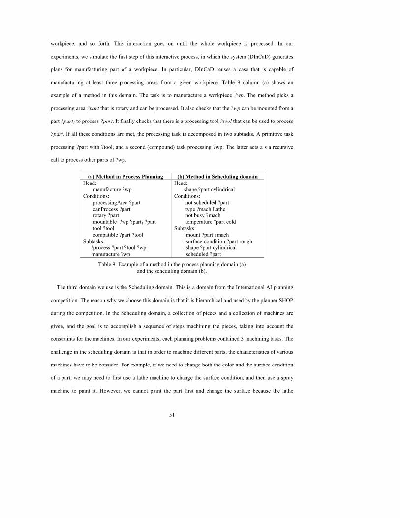
1
Dissertation
August 6, 2006
Case-Based Task Decomposition with Incomplete
Planning Domain Descriptions
By: Ke Xu
Department of Computer Science & Engineering
Lehigh University
Committee Members: Dr. Glenn Blank
Dr. Jeff Heflin
Dr. Héctor Muñoz-Avila (Advisor)
Dr. Rosina Weber
Page 2
2
Abstract........................................................................................................................................................... 5
Chapter One: Introduction and Overview....................................................................................................... 7
1 Introduction ........................................................................................................................................... 7
1.1 Hierarchical Task Network Planning........................................................................................... 7
1.1.1 Case-based Reasoning........................................................................................................ 8
2 Motivation............................................................................................................................................... 9
3 Solution................................................................................................................................................. 11
4 Challenges and Approaches .................................................................................................................. 12
4.1 Research Challenges .................................................................................................................. 12
4.1.1 Planning with Incomplete Task Model............................................................................. 12
4.1.2 Semantics for Case-based Reasoning............................................................................... 13
4.1.3 Evaluating Case-Based Planning Systems ....................................................................... 13
4.2 Approaches ................................................................................................................................ 14
4.2.1 Mechanisms Overview..................................................................................................... 14
4.2.2 Theoretical Analysis......................................................................................................... 16
4.2.3 Empirical Evaluations ...................................................................................................... 16
5 Contributions ........................................................................................................................................ 17
Chapter Two: Preliminaries .......................................................................................................................... 19
1 Case-based Reasoning .......................................................................................................................... 19
2 Hierarchical Task Network (HTN) Planning ........................................................................................ 21
3 Case-Based Task Decomposition.......................................................................................................... 25
3.1 The Knowledge Containers........................................................................................................ 25
3.2 Hierarchical Case Representation .............................................................................................. 26
3.3 Generalized Cases versus Concrete Cases ................................................................................. 28
3.3.1 Differences of Using Concrete and Generalized Cases .................................................... 29
3.3.2 Commonalities of Using Concrete and Generalized Cases .............................................. 31
3.3.3 Motivation of Using Generalized Cases........................................................................... 31
Chapter Three: The DInCaD System............................................................................................................ 33
Page 3
3
1 Overview............................................................................................................................................... 33
1.1 Simple Case Generalization....................................................................................................... 34
1.2 Preference-Guided Case Refinement ......................................................................................... 35
1.2.1 Constant Preference Assignment Phase ........................................................................... 35
1.2.2 Type Preference Assignment Phase ................................................................................. 36
1.2.3 Case Base Maintenance.................................................................................................... 39
1.3 Generalized Case Retrieval........................................................................................................ 41
1.4 Generalized Case Reuse............................................................................................................. 42
2 Properties of DInCaD ........................................................................................................................... 44
3 Empirical Evaluation ............................................................................................................................ 49
3.1 Test Domains ............................................................................................................................. 49
3.2 Experimental Setup.................................................................................................................... 52
3.3 Evaluation Metrics..................................................................................................................... 54
3.3.1 Definitions for Evaluation ................................................................................................ 54
3.3.2 Receiver Operating Characteristic (ROC)........................................................................ 54
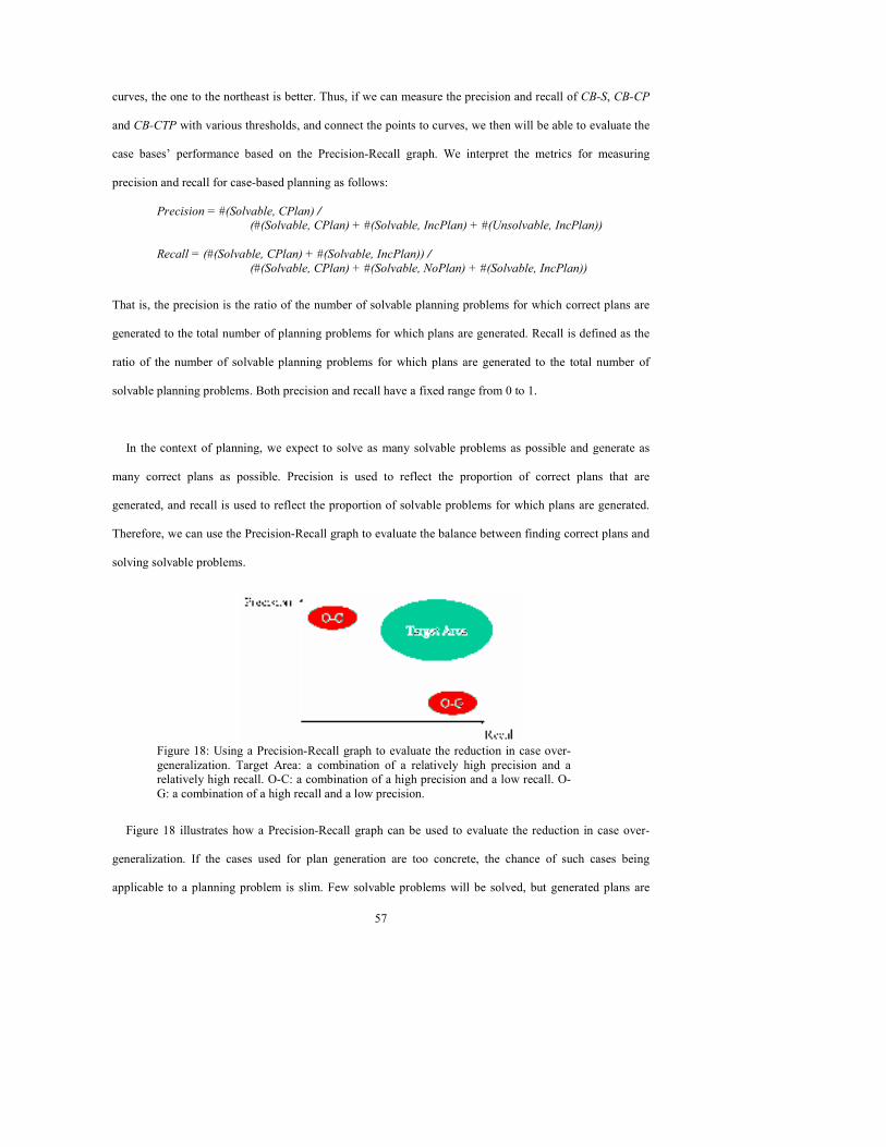
3.3.3 Precision-Recall ............................................................................................................... 56
3.3.4 Relation between Evaluation Metrics and Soundness-Completeness .............................. 58
3.4 Results ....................................................................................................................................... 59
3.4.1 ROC and Precision-recall ................................................................................................. 59
3.4.2 Coverage .......................................................................................................................... 62
Chapter Four: A Practical Application – CaBMA ........................................................................................ 63
1 Introduction........................................................................................................................................... 63
1.1 Project Planning......................................................................................................................... 63
1.2 CaBMA...................................................................................................................................... 64
2 Motivation............................................................................................................................................. 64
3 The CaBMA System............................................................................................................................. 66
3.1 Overview of the System............................................................................................................. 66
3.2 The Gen+ Component................................................................................................................ 67
Page 4
4
3.2.1 Capturing Cases with Gen+.............................................................................................. 67
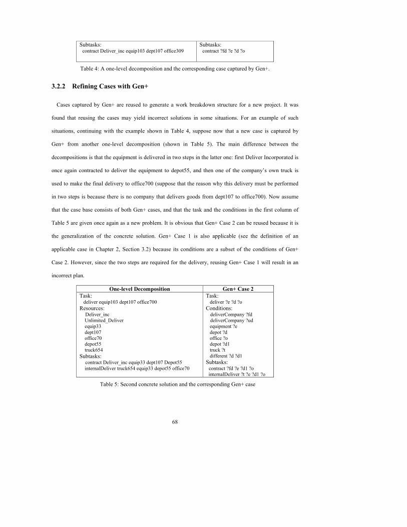
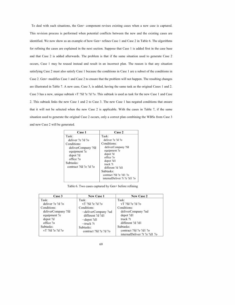
3.2.2 Refining Cases with Gen+................................................................................................ 68
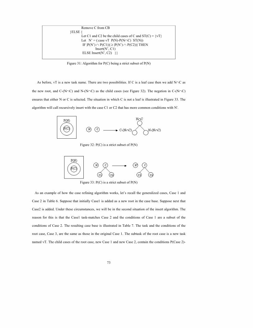
3.2.3 The Case Refining Algorithm .......................................................................................... 70
3.3 The SHOP/CCBR Component................................................................................................... 74
3.4 The Goal Graph Component ...................................................................................................... 75
3.4.1 Case Reuse Inconsistencies .............................................................................................. 75
3.4.2 Mechanism of the Goal Graph Component...................................................................... 77
4 Summary............................................................................................................................................... 82
Chapter Five: Related Work ......................................................................................................................... 83
1 Related Work ........................................................................................................................................ 83
1.1 Case-based Reasoning and Planning ......................................................................................... 83
1.2 Retrieval Criteria in Case-based Planning ................................................................................. 86
1.3 Induction of Domain Descriptions ............................................................................................. 89
Chapter Six: Final Remarks .......................................................................................................................... 91
References..................................................................................................................................................... 93
Appendix A: Proofs of Statements in Section 5, Chapter Three................................................................. 103
Appendix B: Domain Descriptions ............................................................................................................. 109
1. The UM Translog Domain.................................................................................................................. 109
Operators: ........................................................................................................................................... 109
Methods: ............................................................................................................................................. 110
Axioms:............................................................................................................................................... 115
2. The Process Planning Domain ............................................................................................................ 116
Operators: ........................................................................................................................................... 116
Methods: ............................................................................................................................................. 117
Axioms:............................................................................................................................................... 118
3. The Scheduling Domain ..................................................................................................................... 120
Operators: ........................................................................................................................................... 120
Methods: ............................................................................................................................................. 122
Page 5
5
Abstract
Hierarchical task network (HTN) task decomposition is a planning paradigm that
decomposes high-level tasks into simpler ones during problem solving. Over the years, there
has been a recurrent interest on HTN representations for a variety of reasons, including its
relation with models for cognitive reasoning, runtime efficiency, and a number of real-world
domains that are amenable to be modeled in a hierarchical fashion. Despite this interest, an
obstacle that hinders the use of HTN planning techniques in a wide range of applications is
the need for a complete domain description In case-based reasoning (CBR), previous
problem-solving episodes are reused to solve a new problem. A number of research efforts
have been conducted for combining CBR and planning in the past. Some of this research
resulted in domain-independent CBR systems for planning but required a complete domain
description. Others did not require a domain description but resulted in domain-specific
problem solving.
In this dissertation, we report on a novel approach for hierarchical task decomposition with
incomplete domain descriptions, utilizing domain-independent case-based reasoning
techniques. Various techniques for case refinement, retrieval, and reuse are presented,
following the idea of reusing generalized cases for problem solving. These techniques are
integrated in the DInCaD (for: Domain Independent Case-based task Decomposition)
system, which is implemented to deal with situations in which cases are the main source of
task decomposition knowledge. In addition, semantics are defined and proofed for analyzing
the properties of our work, providing a complementary to the theoretical foundation of case-
based reasoning research. Several metrics for evaluating case-based planning systems are
studied and adapted, and are applied to analyze the experimental results of DInCaD. To the
best of our knowledge, DInCaD is the first case-based reasoning system that performs task
decomposition using a domain-independent case adaptation procedure with cases as the main
source of task decomposition knowledge.
Page 7
7
Chapter One: Introduction and Overview
1 Introduction
1.1 Hierarchical Task Network Planning
Hierarchical task network (HTN) planning is an important, frequently studied research topic. Several
researchers have reported work on its formalisms and applications (Wilkins, 1988; Currie & Tate, 1991;
Erol et al., 1994; Smith et al., 1998; Nau et al., 2005). In HTN planning, high-level tasks are decomposed
into simpler tasks until a sequence of primitive actions solving the high-level tasks is generated. There are
three main motivations for the recurrent interest on HTN planning. First, researchers have pointed out that
one way to model how humans acquire knowledge is through a hierarchy of skills. Humans begin by
learning simpler tasks and then proceed by learning the more complex tasks. Thus, hierarchical modeling is
at the core of many cognitive architectures (Choi & Langley, 2005). Second, HTN planning is a natural
representation for many real-world domains, including military planning (Mitchell, 1997), computer games
(Smith et al., 1998; Hoang et al., 2005), manufacturing processes (Nau et al., 1999), project management
(Xu & Muñoz-Avila, 2004), and story-telling (Cavazza & Charles, 2005). Third, HTN planning has played
a fundamental role in the remarkable advances of AI planning research over the past few years. HTN
knowledge representation principles of capturing domain-specific strategies for problem solving while
performing domain-independent search was in part the motivation for the so-called domain-configurable
planners such as SHOP (Nau et al., 1999; 2001), which demonstrated impressive gains of runtime
performance over earlier classical planners. These new paradigms for planning have improved the runtime
performance for solving planning problems by several levels of magnitude. Most of these paradigms allow
domain experts to manually specify domain-specific knowledge in a domain-independent system while
providing well-defined semantics.
Despite these successes, a major hurdle for using AI planning in general, and HTN planning in particular,
is the need for a complete domain description. A domain description is a collection of knowledge
Page 8
8
constructs describing the target domain. In HTN planning, a domain description consists of two parts: the
action model and the task model. The action model encodes knowledge about valid actions or primitive
tasks changing the state of the world. The task model encodes knowledge about how to decompose tasks.
For example, in a possible encoding of the blocks world in HTNs, the action model indicates how to move
individual blocks whereas the task model indicates how to move piles of blocks. Over the last few years,
although research effort has been made on learning and improving domain descriptions for planning
(Zimmerman & Kambhampati, 2003), it was mainly focused on learning the action model. Little attention
has been given on how to learn the task model automatically. The learning problem can be stated as how to
solve a problem in a domain, given a number of solution instances (Martin & Geffner, 2000). The bulk of
research involving planning and learning has focused on learning search control knowledge (e.g., Etzioni,
1993; Minton, 1988; Fern et al., 2004; Botea et al., 2005). Search control knowledge indicates how to use
the domain description to generate a plan efficiently. Some research has been done on building interfaces
for knowledge acquisition (e.g., Blythe et al., 2001), and induction of domain descriptions (e.g., Martin &
Geffner, 2000; McCluskey et al., 2002; Winner & Veloso, 2003). This research concentrates on
acquiring/learning action models, but not on learning task models.
1.1.1 Case-based Reasoning
Case-based reasoning (CBR) “solves new problems by using or adapting solutions that were used to
solve old problems” (Riesbeck & Schank, 1989). One of the motivations of CBR is that in many domains,
cases (i.e., previous problem-solving episodes) are readily available. This is one of the crucial reasons for
successful applications of CBR to help-desk, diagnosis, and prediction tasks (Watson, 1997). Despite these
successes, an obstacle for using CBR in an even wider range of application domains is the difficulty to
develop adequate case reuse techniques. Most CBR applications deal with analysis tasks such as
classification. A reason for this situation is that relatively simple domain-independent case reuse
techniques, such as taking a majority vote of the classification from similar cases, have proven to be
effective (Dietterich, 1997). In contrast, few CBR applications have been developed for synthesis tasks
such as planning. For synthesis tasks, domain-independent case adaptation techniques exist (e.g., Veloso &
Carbonell, 1993; Hanks & Weld, 1995; Bergmann & Wilke, 1995; Ihrig & Kambhampati, 1997; Gerevini
Page 9
9
& Serina, 2000; Tonidandel & Rillo, 2005) but require complete domain descriptions, which are not
available in many domains. An alternative is to develop domain-specific case adaptation techniques.
However, developing such techniques is also frequently unfeasible because of the large knowledge
engineering effort involved.
2 Motivation
Our work is motivated by situations in which hierarchical cases are readily accessible, but neither task
models nor case adaptation knowledge is available. An example of such a situation is project planning. The
Project Management Institute’s A Guide for the Project Management Body of Knowledge (PMI, 1999)
defines a project as an endeavor to create a unique product or to deliver a unique service. Unique means
that the product or service differs in some distinguishing way from similar products or services (Anderson
et al., 2000). Examples of projects include dam constructions and enterprise-wide software systems
development. Project planning generates plans for providing business products and services under time and
resources constraints, comprising the following knowledge/work activities and decisions (PMI 1999):
1. Creating a work breakdown structure (WBS): The (human) planner identifies and establishes a
hierarchically organized collection of tasks that enables the delivery of required products and services.
2. Identifying/incorporating task dependencies: The planner identifies task dependencies and schedules
tasks accordingly.
3. Estimating task and project durations: The planner estimates the time required to accomplish each task,
and uses the task dependencies in the WBS to estimate overall project duration.
4. Identifying, estimating, and allocating resources: The planner identifies the types of resources required
by each task, allocates the resources to each task in the WBS, and estimates the rates of resource
consumption.
5. Estimating overall project costs/budget: The planner estimates the cost of resources consumed, compiles
an overall project cost, and often derives a scheduled cash flow.
6. Estimating uncertainties and risks: The planner estimates uncertainties and risks associated with tasks,
resources, and schedules.
Page 10
10
Software packages for project management are commercially available, including Microsoft Project™
(Microsoft), SureTrak™ (Primavera Systems Inc.), and Autoplan™ (Digital Tools Inc.). Figure 1 shows a
work breakdown structure of a manufacturing project represented in Microsoft Project™. The compound
tasks, for example, “Manufacturing Workpiece wp353”, are decomposed into simpler subtasks. The
subtasks, such as “Processing Ascending Outline ao2 on Workpiece wp353”, are eventually decomposed
into activities, which are basic executable work units (i.e., primitive tasks). For instance, “Machining
Processing Area p3 with Tool t54” is an activity. They help a planner with manually recording his/her plan
with the activities above involved. These packages do provide support to ensure that resources are not over-
allocated (activity (4) from the project planning activities), to estimate costs (activity (5)) by adding up
costs for tasks, and to estimate global times (activity (3)) by adding up times from leaf tasks. However, they
do not assist a planner in the complicated and knowledge intensive part of project planning: creating a
WBS and identifying dependencies between the tasks.
Figure 1: A WBS in Microsoft ProjectTM
Project planning covers several practical domains, such as research proposal development, public events
organization, and civil construction management. In project planning, previous project plans are accessible
and can be represented as HTNs (Mukkamalla & Muñoz-Avila, 2002; Xu & Muñoz-Avila, 2005).
However, master principles for generating new project plans are not available, and it is hard to obtain users’
Page 11
11
strategies and knowledge for plan adaptation. The primary planning activity of a project involves creating a
WBS for it, which requires decomposing the project’s tasks into manageable work units. This process
requires significant domain knowledge and experience. For example, a software project manager who
needs to deliver a real time chemical process control system must employ significant knowledge of real-
time software development processes combined with experience in chemical process control. The complex
interdependencies between task and domain knowledge make creating the WBS a difficult task.
Knowledge-based project planning advocates assisting project planners in the creation of work breakdown
structures, intelligent planning systems could significantly expedite the planning process and increase its
chances of success (Muñoz-Avila et al., 2002). As starting point, it has been observed that there is a
mapping between hierarchical task networks (HTN) representations and WBS representations (Muñoz-
Avila et al., 2002). Therefore, is possible to use HTN planning techniques to generate WBSs automatically.
The main difficulty is that neither task models nor WBS adaptation techniques are available. However,
cases, representing previously generated WBSs, are readily available. In fact, Mukkamalla and Muñoz-
Avila (2002) describe a procedure that is capable of capturing cases from a WBS such as the one
represented in Figure 1. This is the starting assumption for DInCaD, where cases capturing knowledge
about how to decompose tasks are given as input.
3 Solution
In this dissertation, the idea of case-based hierarchical task decomposition is presented, utilizing various
case-based reasoning techniques to solve the limitation of HTN planning with incomplete domain
descriptions. With the absence of a task model, generalized cases are captured from previous problem-
solving episodes as part of the domain knowledge. A preference-guided case refinement is applied to
reduce case over-generalization (i.e., situations in which using generalized cases yields incorrect plans). For
the same purpose, a similarity criterion that takes advantage of the refinement is designed and used during
case retrieval. A hierarchical task network (HTN) planning algorithm performs case reuse and generates
plans for new problems. To conduct theoretical analysis on our method, we give semantic definitions and
make property statements, which are complementary for the theoretical foundation of case-based reasoning.
Page 12
12
In the context of case-based planning, the meaning and importance of planning quality is also studied,
followed by two evaluation metrics customized for measuring the reduction of case over-generalization.
The DInCaD (for: Domain Independent Case-based task Decomposition) system, as an implementation
of case-based hierarchical decomposition with incomplete task model, is presented in the dissertation.
DInCaD encompasses the procedures of case refinement, retrieval, and reuse. It combines a case refinement
procedure with a case similarity criterion to reduce case over-generalization (i.e., situations in which using
generalized cases yields incorrect plans). Retrieved generalized cases are reused to solve new problems, in
a domain independent HTN planning fashion. We performed experimental evaluations on DInCaD to
measure the reduction on case over-generalization. We also semantically analyzed the theoretical properties
of the system. To our best knowledge, DInCaD is the first case-based reasoning system that performs task
decomposition using a domain-independent case adaptation procedure with incomplete domain
descriptions.
4 Challenges and Approaches
4.1 Research Challenges
4.1.1 Planning with Incomplete Task Model
Our work is motivated by domains in which cases are readily available but neither domain descriptions
nor case adaptation knowledge is available. An example is project planning, which is usually used during
project management. Several software systems for project planning are commercially available (e.g.,
Microsoft ProjectTM by Microsoft, and SureTrak™ by Primavera Systems Inc). These systems provide
functionalities for editing work-breakdown structures (WBS), which indicate how complex tasks can be
decomposed into simple work units. However, these systems cannot perform synthesis planning
automatically. The planning process has to be done manually by the users. Research has shown that
decompositional representation can be used for knowledge representation in CBR (Muñoz-Avila et al.,
2001). Therefore, we can use case-based reasoning with hierarchical knowledge representation to
Page 13
13
accomplish task decomposition in a HTN planning manner. With such case-based task decomposition
technique, the systems are able to perform synthesis planning automatically with incomplete domain
descriptions (i.e., a possibly empty task model), by adapting and reusing cases.
4.1.2 Semantics for Case-based Reasoning
Although significant research has been done on case-based reasoning, the need for enhancing the
theoretical foundation of CBR still exists (Muñoz-Avila et al., 2005). There are yet no generic semantics
formally defined or widely accepted for case-based reasoning, including essential concepts such as
soundness, completeness and coverage. In our work, we defined complementary semantics for case-based
reasoning, and used the semantics to theoretically analyze the properties of the DInCaD system.
4.1.3 Evaluating Case-Based Planning Systems
Several evaluation metrics have been proposed to measure the performance of a case-based reasoning
system. For example, the comparative utility analysis (Francis & Ram, 1995) measures how well a CBR
system deals with the utility problem (Minton, 1988), in which having more knowledge to improve
reasoning may end up degrading the performance; the plan quality metrics (Perez & Carbonell 1994)
concentrate on measuring the execution cost of the solutions, such as the number of steps in a solution, the
execution time, and the resources used; the convergence evaluation metric (Ilghami, et al., 2005) measures
the number of cases needed and the CPU time used by a CBR system to converge, using version space
(Mitchell, 1977).
However, there are few evaluation metrics that evaluate a case-based reasoning system’s performance on
synthesis tasks (e.g., HTN planning). For instance, in the context of case-based planning, solving a
planning problem correctly means either finding a valid plan for a solvable problem, or recognizing an
unsolvable problem. Therefore, when we evaluate the problem-solving capability of a planning system,
both situations should be considered. In addition, using a case-based planning system, we expect to solve as
many problems as possible, and meanwhile, to generate as many correct plans as possible. Thus, it is
necessary to evaluate the balance between satisfying the both requirements. In our work, we proposed
evaluation metrics for measuring planning qualities of case-based planning systems.
Page 14
14
4.2 Approaches
4.2.1 Mechanisms Overview
For HTN planning with an incomplete task model, our approach receives as input a complete action
model, a collection of cases (e.g., cases obtained from episodes of previous valid project plans), and a type
ontology (i.e., a set of type-subtype relations). The generalizations of the cases are stored in the case base.
To reduce case over-generalization, preferences for refining the generalized cases are automatically learnt,
referencing the type ontology. Given a new planning problem, similarities of cases are computed using a
similarity criterion that takes advantage of the previous refinement. A case-based HTN planning algorithm
adapts and reuses the most similar cases to solve the problem.
Case Refinement
To reduce case over-generalization, generalized cases are refined with the learnt preferences. We have
found two kinds of opportunities for such case refinement: with both type preferences and constant
preferences. Type preferences are learnt, generated, and added to generalized cases to eliminate type
conflicts. A type conflict indicates that some applicability conditions in a generalized case are more
specific than those in another generalized case, referencing to the type ontology. It implies that if both cases
can be reused to accomplish a planning task, reusing either case does not always guarantee correct plans.
During the case refinement, type conflicts between generalized cases are automatically detected. Refined
with type preferences, generalized cases that are more specific than others will be prioritized during case
retrieval. The goal of adding type preferences is to reduce case over-generalization by preferring the
specificity of a generalized case to its generality. In addition to type preferences, constant preferences are
also used to refine generalized cases. Constant preferences are automatically extracted from the concrete
case that has been used to obtain the generalized case. With constant preferences, it is ensured that the
refined cases have a restricted form of soundness.
Page 15
15
Case Retrieval
During the process of case retrieval, the generalized cases are ranked according to their similarity values
to the problem. A similarity criterion is designed to implement the bias that the more similar a case is to a
problem, the more likely the case will be retrieved. The reason behind this bias is that higher ranked cases
are preferred since they represent a recommendation of the system of the more suitable cases for a
particular situation (Aha et al., 1998). The highest ranked case(s) will be retrieved, and be reused by an
HTN planning algorithm to generate a plan for the problem.
Automatic case-based reasoning, such as our approach presented in this dissertation, usually selects the
highest ranked case during retrieval, according to the given problem description. In contrast, a
conversational case-based reasoning (CCBR) system provides users a list of ranked cases to choose, and
does not expect a complete problem description (Aha et al., 2001). The user can initially input brief textual
description of a problem. A CCBR system requires interactions (conversations) with the user to determine
the similarities between cases and the query. The interactions are of a question-answering manner: the
system prompts the user with a list of cases according to the problem description, and displays a set of
questions for each case. The similarities of the cases will be determined by the user’s answers to the
questions. The system updates and re-ranks the list of cases after each time having conversations with the
user, until eventually the user decides which case should be reused for reasoning.
Case Reuse
Once a generalized case gC is retrieved for a planning task t, gC is reused in standard HTN planning
fashion. If θ is a substitution fulfilling the applicability requirement of gC, t is decomposed with the
subtasks θST, where ST is the solution in gC. The task decomposition process continues recursively with
the subtasks until primitive tasks referred by the action model are obtained. The action model is also
required for stating the correctness of obtained plans, which is necessary for the theoretical analysis and
empirical evaluation. Nevertheless, in particular situations such as project planning, the decompositions can
Page 16
16
still be obtained and viewed as WBSs for planning tasks, even with the fact that the action model may be
absent.
4.2.2 Theoretical Analysis
We give definitions in order to analyze the theoretical properties of our approach. Using these
definitions, we are also able to provide well-defined semantics that are complementary to the theoretical
foundation of case-based reasoning. The definitions consist of important concepts such as:
1. Soundness: A case base CB is sound relative to a set of concrete problem-solution pairs PS = (p1, s1),
(p2, s2), …, (pn, sn), if and only if whenever pi (1≤ i ≤ n) is given again as a problem, the solution generated
using CB could also be generated using PS as the case base.
2. Completeness: A case base CB, generalized from a set of concrete problem-solution pairs PS = (p1,
s1), (p2, s2), …, (pn, sn), is complete relative to PS, if and only if whenever pi (1≤ i ≤ n) is given again as a
problem, the solutions generated using CB contain si.
3. Coverage: The coverage of a case base CB with respect to an incomplete domain description I is the
number of solvable planning problems that can be solved using CB and I.
4.2.3 Empirical Evaluations
Case over-generalization is a major limitation to the planning qualities, because it may result in incorrect
plans. For the presented approach, we conducted experiments on planning domains to evaluate its
performance on reducing this limitation. Two evaluation metrics are used through the experiments. The
Receiver Operating Characteristic (Provost and Fawcett, 2001) graph is used to evaluate the problem-
solving capability of a planning system, with the consideration of either finding a valid plan for a solvable
problem, or recognizing an unsolvable problem. The Precision-Recall (Salton et al., 1975) graph is used to
measure the balance between finding correct plans and solving problems. In the dissertation, both of the
classic metrics, which are not restricted to case-based reasoning (e.g., such metrics are also used for
evaluation purposes in Information Retrieval and Machine Leaning), are carefully examined and properly
adapted in the context of case-based planning, and applied to evaluate the reduction on case over-
generalization in our work.
Page 17
17
5 Contributions
We summarize our contributions as follows:
1. To the best of our knowledge, the presented work is a novel approach for hierarchical task
decomposition with incomplete domain descriptions, utilizing domain-independent case-based
reasoning techniques. It provides a solution to the limitation of case over-generalization, which is
a consequential side effect of using generalized cases for case-based reasoning.
2. We generalize cases to improve coverage (i.e., the collection of problems that can be solved). We
introduce a preference-guided case refinement procedure, and a retrieval criterion that takes
advantage of the refinement to reduce case over-generalization.
3. We introduce a theoretical basis to analyze case-based reasoning systems.
a) First, we define a notion of relative soundness.
b) Second, we extend the notion of coverage of a case base to include knowledge bases
consisting of incomplete domain descriptions (i.e., with possibly empty task models) and
cases.
c) Third, we state a relation between the coverage of the knowledge base in a case-based
reasoning system and its relative soundness.
The conclusions derived from the analysis are complementary to the semantic foundation of case-
based reasoning.
4. We introduce an empirical basis to analyze planning quality.
a) We adapt the Receiver Operating Characteristic, a traditional metric for classification tasks, to
evaluate the performance in case-based planning.
b) We adapt Precision-Recall, a traditional metric for Information Retrieval, to evaluate the
performance in case-based planning.
c) We analyze how these adapted metrics contribute to measure the reduction in case over-
generalization.
The adapted evaluation metrics provide an instructive perspective on measuring planning quality of
generic case-base planning systems.
Page 18
18
The rest of the document will be organized as following: in chapter two, we give the preliminaries
involved: section 1 is case-based reasoning, section 2 is HTN planning, section 3 is case-based task
decomposition, and section 4 is using generalized cases. In chapter three, section 1 is the overview of the
DInCaD system; section 2 is the analysis on the system’s theoretical properties; section 3 is the
experimental evaluation. In chapter four, we introduce a practical application of our work: the CaBMA
system. It is a case-based planning assistant built on top of a commercial project management software,
Microsoft ProjectTM. CaBMA was made to assist the user to generate and refine plans for project
management. In chapter five, we discuss the related work within three research areas: case-based reasoning
and planning, retrieval criteria used in case-based planning, and induction of domain descriptions. In the
final remarks in chapter six, we summarize the features of DInCaD and its research contributions. We also
point out several interesting potential research directions we came up with, based on the research and
observation on DInCaD. Appendix A is the proofs of the theoretical statements made to DInCaD. Appendix
B provides the domain descriptions of the three domains used for experiments.
Page 19
19
Chapter Two: Preliminaries
1 Case-based Reasoning
Case-based reasoning (CBR) reuses previous solutions to solve new problems. Figure 2 shows a classical
case-based reasoning cycle (Aamodt & Plaza, 1994). In CBR, a case is assumed to consist of a problem
part and a solution part (Breslow & Aha, 1997). The problem part records the description of the problem
that is being solved. The solution part records how to solve the problem. The CBR cycle takes as inputs a
description of a problem, a set of cases, and a collection of general knowledge.
Figure 2: The case-based reasoning cycle (Aamodt & Plaza, 1994)
During the retrieve step, the most similar case to the problem will be selected from the case base. The
similarity of a case to a problem is determined by the similarity between the description of the problem part
of the case and the description of the input problem. The assumption is that the more similar the problem
and the case are, the less adaptation effort reusing the case will require for solving the problem.
During the reuse step, the solution part of the retrieved case will be either simply reused, or adapted and
then reused to provide a suggested solution to the input problem. There are two major ways to adapt a
Page 20
20
retrieved case: transformation adaptation and derivational adaptation (Watson & Marir, 1994).
Transformation adaptation requires domain-dependent knowledge to transform the solution of the retrieved
case into the solution of the new case. In the derivational adaptation, the solution of the retrieved case is
used to guide the replay of decisions that were made during the process of solving the problem in the
retrieved case. Derivational adaptation then reuses these decisions to replay the solutions from reusable
cases, returns a solution to the input problem, if any, or indicates a failure.
During the revise step, the suggested solution to the input problem will be tested in the real world
environment, or in a simulation of the environment. If the solution is not correct, an explanation of the
incorrectness will be generated, and the solution will be repaired with domain knowledge. If the solution is
confirmed, a new case will be obtained.
During the retain step, the case base is updated with the newly obtained case. In this step, necessary
information from the obtained case will be extracted. Also should be decided is how to index the cases for
further retrieval.
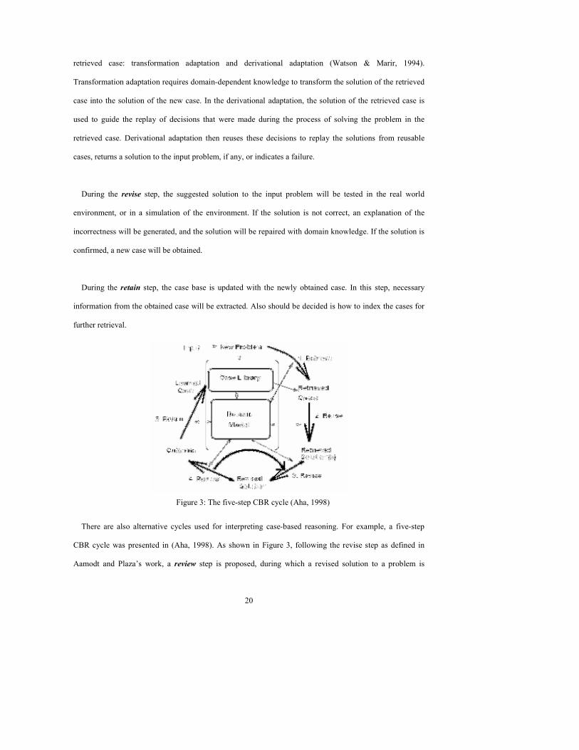
Figure 3: The five-step CBR cycle (Aha, 1998)
There are also alternative cycles used for interpreting case-based reasoning. For example, a five-step
CBR cycle was presented in (Aha, 1998). As shown in Figure 3, following the revise step as defined in
Aamodt and Plaza’s work, a review step is proposed, during which a revised solution to a problem is
Page 21
21
evaluated. The solution will be retained as a new case if the outcome of the evaluation is acceptable.
Otherwise, the solution requires further revision. Another example is the six-step CBR cycle presented in
(Watson, 2001), in which the refine step is introduced, as shown in Figure 4. During the refine step, the
indexes of the case base and feature weights are updated when a new case is retained.
Figure 4: The six-step case-based reasoning cycle (Watson, 2001)
2 Hierarchical Task Network (HTN) Planning
Hierarchical task network (HTN) planning is a plan generating method, in which complex tasks are
decomposed into simple tasks for accomplishment. HTN planning achieves complex tasks by decomposing
them into simpler subtasks. Planning continues by decomposing the simpler tasks recursively until tasks
representing concrete actions are generated. These actions compose a plan achieving the high-level tasks.
In addition to obtaining these plans, we are also interested in the task hierarchy that led to these plans
because the task hierarchy is a WBS in project planning.
The main knowledge artifacts that indicate how to decompose tasks are called methods. A method, M, is
a 3-tuple (h, Q, ST), such that: h, called the head of M, is the task being decomposed; Q, called the
conditions, is the list of requirements for using the method; and ST are the subtasks achieving h. Figure 5
shows a simple example of a method from the logistics transportation domain (Veloso, 1994). Variables are
preceded with a question mark. For example, ?e4 indicates a variable. Primitive tasks are preceded with an
exclamation mark. For example, !load ?e4 ?t1 ?d6 is a primitive task. The task been achieved is to deliver an
Page 22
22
object (?e4) from an initial location (?d6) to a destination (?d7). This method has two preconditions and
three primitive subtasks. These preconditions require that the object to be delivered be at the initial
location, and that a truck (?t1) to be in the same location as where the object is located. The subtasks consist
of loading the object in the truck (since they are in the same location), driving the truck from the initial
location to the destination, and unloading the object at the destination.
Head:
deliver ?e4 ?d6 ?d7
Conditions:
at ?e4 ?d6
at ?t1 ?d6
Subtasks:
!load ?e4 ?t1 ?d6
!drive ?t1?d6 ?d7
!unload ?e4 ?t1 ?d7
Figure 5: A method in the UM Translog Domain
To achieve a task that can be decomposed (called a compound task), an HTN planner searches for
applicable methods. A method M is applicable to a compound task t, relative to a state S (a set of ground
atoms), iff match(h, t) (i.e., h and t have the same predicate and arity, and a consistent set of bindings Θ
exists, which maps variables to constants so that all terms in h match their corresponding ground terms in t)
and Q are satisfied by S (i.e., there exists a consistent extension Θ' of Θ such that for every single condition
q∈Q, qΘ'∈S, and for every condition not(q)∈Q, qΘ'∉S). Let t be a task, S be a state, and M = (h, Q,
ST) be an applicable method relative to S. The result of applying M to t is a task list R = (STΘ)Θ', called a
reduction of t. Table 1 shows an example of a compound task and state. The method in Figure 5 is
applicable to this task relative to this state by using the variable bindings: ?e4 object1, ?d6 location0,
?d7 location1, and ?t1 truck2. Table 1 also shows the resulting reduction from applying the method
with these bindings.
Compound Task deliver object1 location0 location1
State at truck2 location0
at object1 location0
Reduction !load object1 truck2 location0
!drive truck2 location0 location1 !unload object1 truck2 location1
Table 1: Compound task, state and reduction
Page 23
23
To achieve a task t that represents an atomic action (called a primitive task), an HTN planner uses
operators. An operator O is of the form (h, AL, DL), such that h (the head of O) is a primitive task, and AL
and DL are the so-called add-list and delete-list (sets of atoms). Unlike in STRIPS planning, operators in
HTN planning do not have applicability conditions. The reason is that these conditions are already
evaluated in the methods. Figure 6 shows a simple example of an operator from the transportation domain.
The primitive task is to load the truck (?t1) with the object (?e4) at the location (?d6). The add-list indicates
that when the operator is applied to achieve the primitive task, the object will be at the truck. The delete-list
indicates that when the operator is applied, the object will be no longer at the location.
Head:
!load ?e4 ?t1 ?d6
Add-list:
at ?e4 ?t1
Delete-list:
at ?e4 ?d6
Figure 6: An example of an operator.
An operator O is applicable to a primitive task t, relative to a state S, iff match(h, t). The add-list and
delete-list define how the applicable operator will transform the current state S when applied: every atom in
AL is added to S and every atom in DL is removed from S. When O is applied to t, the instantiated head h’
is called a simple plan to t, and the result of applying O to t is a new state denoted as result(S, h’). Table 2
shows an example of a primitive task, a simple plan to the task, and the changes on the state. The operator
in Figure 6 is applicable to the primitive task, with the following bindings: ?e4 object1, ?t1 truck2, ?d6
location0. If the operator is applied, its head is instantiated according to the bindings, and becomes a
simple plan to the task. The add-list and the delete-list are also instantiated. The resulted atom at object1
truck2 is added to the current state, and the atom at object1 location1 is removed from the current state.
Primitive Task !load object1 truck2 location0
Simple Plan !load object1 truck2 location0
Added to the state at object1 truck2
Deleted from the state at object1 location0
Table 1: Primitive task, simple plan, and changes to state
A planning problem is a 3-tuple (T, S, D), where T is a set of tasks, S is a state, and D is a domain
description -- a collection of methods (the task model) and a collection of operators (the action model). A
problem is solvable if there is a plan that solves it. A plan is a sequence of simple plans. Informally, given
Page 24
24
a planning problem (T, S, D), a plan that recursively achieves all tasks in T, is called a correct plan to the
planning problem (Nau et al., 1999). Besides generating a plan plans for a planning problem, we are also
interested in hierarchical task network (HTN) that led to the plan. Formally, an HTN is defined as follows:
• An expression of the form (th,(t1,…,tm)) is a HTN, where t
h, t1,…,tm with m ≥ 0, are tasks
(a task is represented as a logical atom). Tasks are achieved in the order they are listed.
• An expression of the form (th,(T1,…,Tm)) is a HTN, where t
h is a task and T1,…,Tm are
HTNs. The task network indicates that th is decomposed into T1,…,Tm.
During HTN planning, HTNs are generated. A compound task th is decomposed into subtasks t1,…,tm, by
using methods or cases as indicated before. A primitive task th is achieved by applying an operator, which
changes the state of the world. The process fails if all possibilities are exhausted and there is either always a
compound task for which no method is applicable or a primitive task for which no operator is applicable. If
the process succeeds, an HTN is generated in which every compound task is decomposed and every
primitive task is solved using an operator. The plan can be obtained by performing a pre-order traversal of
the resulting HTN collecting all primitive tasks along the way. In Section 5.4 we will present the HTN
planning algorithm used by DInCaD.
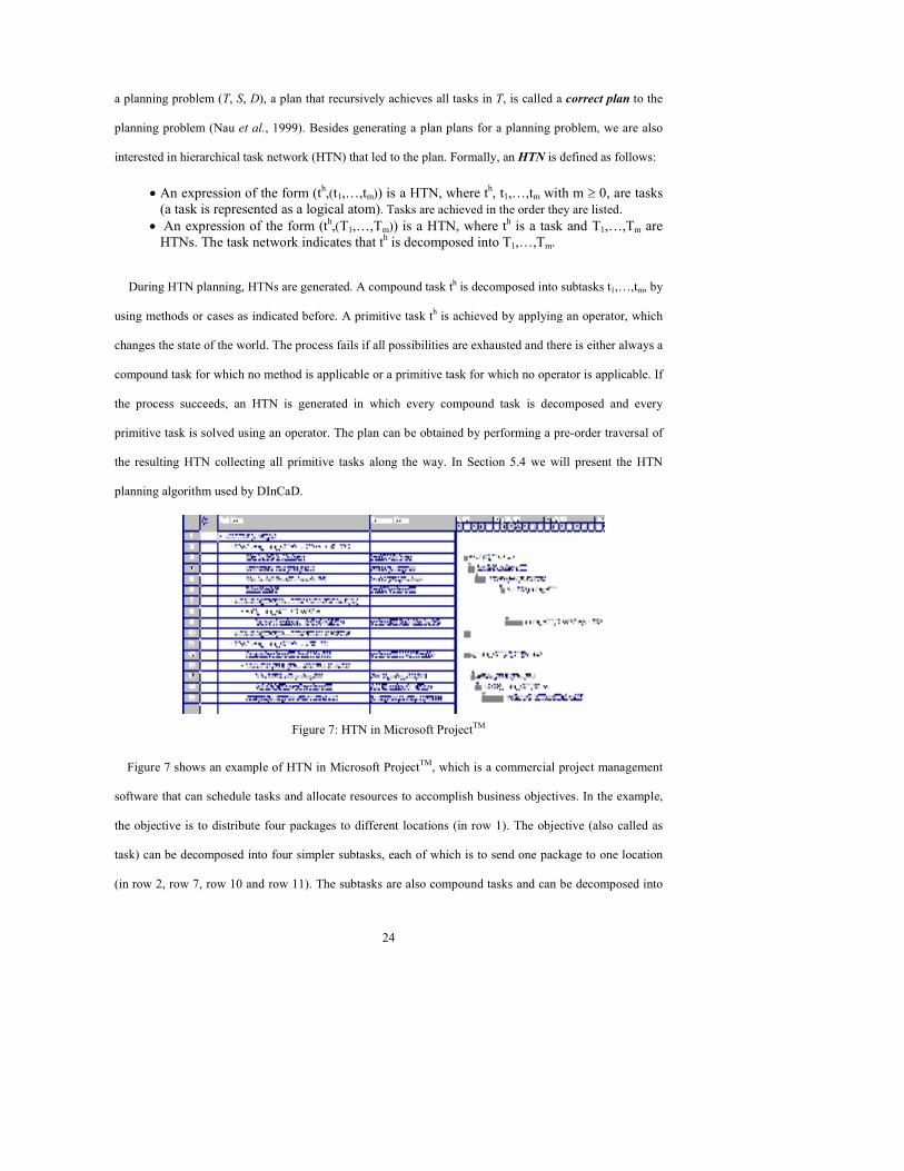
Figure 7: HTN in Microsoft ProjectTM
Figure 7 shows an example of HTN in Microsoft ProjectTM, which is a commercial project management
software that can schedule tasks and allocate resources to accomplish business objectives. In the example,
the objective is to distribute four packages to different locations (in row 1). The objective (also called as
task) can be decomposed into four simpler subtasks, each of which is to send one package to one location
(in row 2, row 7, row 10 and row 11). The subtasks are also compound tasks and can be decomposed into
Page 25
25
primitive subtasks. For instance, the subtask “Distribute package100 from Allentown to NYC” in row 2 is
decomposed into four primitive subtasks, from row 3 to row 6. When the objective is completely
decomposed into primitive subtasks, it can be accomplished by applying fundamental actions on those
primitive subtasks.
3 Case-Based Task Decomposition
3.1 The Knowledge Containers
In 1995, Richter proposed the framework of the four knowledge containers for case-based reasoning
systems: vocabulary, case base, case adaptation knowledge and similarity measures. A knowledge
container is a collection of knowledge that is relevant to multiple tasks in a certain domain (Roth-
Berghofer, 2004). Figure 8 shows the four knowledge containers for case-based reasoning systems. The
vocabulary container contains knowledge required to define a CBR system (e.g., syntax and semantics).
The case base container stores previous problem-solving experiences as cases. The similarity measures
container defines what kind of cases are considered useful and how should the similarity be calculated. The
adaptation knowledge container defines knowledge on how a case can be adapted to solve a problem.
Figure 8: The four knowledge containers for
case-based reasoning systems (Roth-Berghofer, 2004)
This framework for case-based reasoning systems provides flexibility for transforming knowledge.
Transforming knowledge can be seen as either changing the content of a container locally, or shifting the
Page 26
26
knowledge from one container to another. First, content in each container can be changed locally, without
affecting the content in the other containers. For instance, updating the case base with new cases does not
necessarily require changing the adaptation knowledge or similarity criterions. On the other hand, various
similarity criterions can be put into the similarity measures container and later on applied to the same case
base. Second, knowledge in one container can be shifted into another container. For example, if the case
base contains sufficient cases covering the domain, the similarity criterions could be very simple (e.g.,
matching a problem with one of the cases) and no adaptation knowledge would be needed for reasoning.
On the other hand, if we have the complete knowledge on how to adapt cases to solve any given problem,
the knowledge of similarity measures would not be necessary.
As a case-based reasoning system for hierarchical task decomposition, DInCaD fits in the four
containers framework. The vocabulary that defines DInCaD follows the syntax and semantics that are used
in the SHOP (Nau et al. 1999). The case base contains cases that are acquired from the previous problem
solving. DInCaD applies a sequence of processes (e.g., generalization and refinement, which will be
explained in detail in Chapter three) on the cases, so that a relatively simple but effective similarity
criterion is able to take advantage of the processes. In addition, DInCaD performs case-based reasoning
procedures (e.g., case retrieval and reuse, which will be explained in Chapter three) with the case base,
resulting in shifting the adaptation knowledge into the case base container. By these means, DInCaD is able
to work with domains in which cases are accessible, but neither a complete domain description nor domain-
specific case adaptation knowledge is available.
3.2 Hierarchical Case Representation
Research has shown that decompositional representation can be used for knowledge representation in
CBR (Muñoz-Avila et al., 2001). Therefore, case-based hierarchical task decomposition can be seen as a
procedure that uses case-based reasoning with hierarchical representation to accomplish task decomposition
for HTN planning. This procedure combines the principles of HTN planning as in the SHOP system (Nau
et al. 1999) and case reuse as in the SiN system (Muñoz-Avila et al. 2001).
Page 27
27
A case C has the same form as a method, (h, Q, ST). The only difference is that in a case, the task h, the
tasks in ST, and the conditions in Q are all ground (i.e., containing no variables). The rationale is that cases
capture concrete problem-solving episodes (e.g., how did we organize a public concert). Figure 9 shows an
example of a case in the transportation domain. Cases can also be used to decompose compound tasks. A
case C is applicable to a compound task t, relative to a state S, iff h and t are identical, and the conditions in
Q are satisfied by S (i.e., ∀q∈Q q∈S and ∀not(q)∈Q q∉S). The result of using C to decompose t is a
reduction R = ST of t. For example, the case shown in Figure 9 is applicable to the compound task relative
to the state in Table 1. If the case is applied, the same reduction as in Table 1 will be obtained.
Head:
deliver object1 location0 location1
Conditions:
at truck2 location0
at object1 location0
Subtasks:
!load object1 truck2 location0
!drive truck2 location0 location1 !unload object1 truck2 location1
Figure 9: An example of a case.
We assume that a type ontology is available. This assumption is also motivated by project planning,
where both cases and type ontologies are frequently available (Xu & Muñoz-Avila, 2004). We define a
type ontology Ω as a collection of relations in a target domain. These relations can be of two forms: v isa v’
and ?x type: v. The relation v isa v’ indicates that a type v is a subtype of another type v’. The relation ?x
type: v indicates that a variable ?x is of a type v. For example, in the transportation domain that have been
using, we have two types of trucks and objects: trucks with normal a tanker, and trucks with a refrigerating
tanker; normal liquid and perishable liquid. Table 3 shows examples of relations in the type ontology.
RefrigTanker isa Tanker indicates that a refrigerating tanker is also a type of tanker, ?t type: RefrigTanker
means that the object ?e is of type perishable liquid. These relations extend the applicability of cases and
methods. For instance, if a method has a precondition: ?truck1 type: Tanker, the atom truck2 type:
RefrigTanker is in the current state, and RefrigTanker isa Tanker is defined in the type ontology, then the
precondition can be instantiated as truck2 type: Tanker, by applying the binding: ?truck1 truck2.Since
Page 28
28
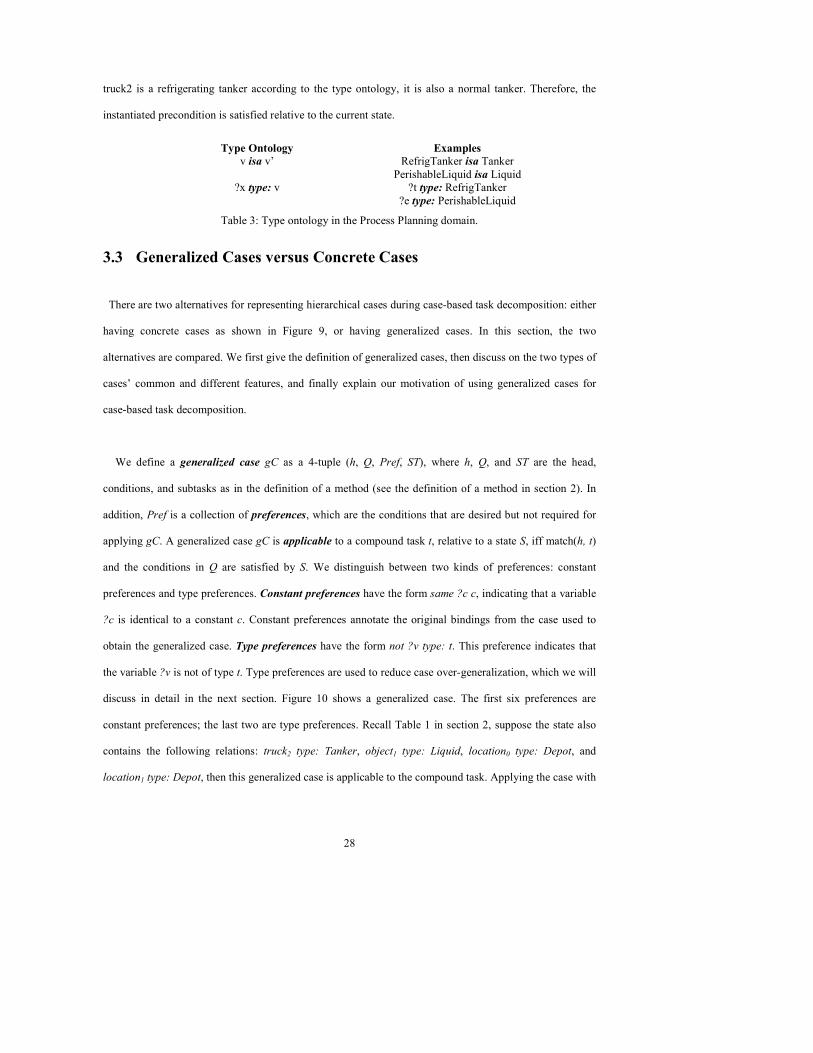
truck2 is a refrigerating tanker according to the type ontology, it is also a normal tanker. Therefore, the
instantiated precondition is satisfied relative to the current state.
Type Ontology Examples
v isa v’ RefrigTanker isa Tanker
PerishableLiquid isa Liquid
?x type: v ?t type: RefrigTanker
?e type: PerishableLiquid
Table 3: Type ontology in the Process Planning domain.
3.3 Generalized Cases versus Concrete Cases
There are two alternatives for representing hierarchical cases during case-based task decomposition: either
having concrete cases as shown in Figure 9, or having generalized cases. In this section, the two
alternatives are compared. We first give the definition of generalized cases, then discuss on the two types of
cases’ common and different features, and finally explain our motivation of using generalized cases for
case-based task decomposition.
We define a generalized case gC as a 4-tuple (h, Q, Pref, ST), where h, Q, and ST are the head,
conditions, and subtasks as in the definition of a method (see the definition of a method in section 2). In
addition, Pref is a collection of preferences, which are the conditions that are desired but not required for
applying gC. A generalized case gC is applicable to a compound task t, relative to a state S, iff match(h, t)
and the conditions in Q are satisfied by S. We distinguish between two kinds of preferences: constant
preferences and type preferences. Constant preferences have the form same ?c c, indicating that a variable
?c is identical to a constant c. Constant preferences annotate the original bindings from the case used to
obtain the generalized case. Type preferences have the form not ?v type: t. This preference indicates that
the variable ?v is not of type t. Type preferences are used to reduce case over-generalization, which we will
discuss in detail in the next section. Figure 10 shows a generalized case. The first six preferences are
constant preferences; the last two are type preferences. Recall Table 1 in section 2, suppose the state also
contains the following relations: truck2 type: Tanker, object1 type: Liquid, location0 type: Depot, and
location1 type: Depot, then this generalized case is applicable to the compound task. Applying the case with
Page 29
29
the bindings: ?e1 object1, ?d2 location0, ?d3 location1, ?t5 truck2 will result in the same
reduction to the task as in Table 1.
Head:
deliver ?e1 ?d2 ?d3
Conditions:
?t5 type: Tanker
?e1 type: Liquid
?d2 type: Depot
?d3 type: Depot
at ?t5 ?d2
at ?e1 ?d2
Preferences:
same ?t5 t5
same ?e1 e1
same ?d2 d2
same ?d3 d3
not ?t5 type: refrigTanker
not ?e1 type: perishableLiquid
Subtasks:
!load ?e1 ?t5 ?d2
!drive ?t5 ?d2 ?d3
!unload ?e1 ?t5 ?d3
Figure 10: A generalized case.
The concept of generalized cases has been presented in many other researches on case-based reasoning
(Kolodner, 1980; Bareiss, 1989; Salzberg, 1991). Using generalized cases is a way to deal with domains
with continuous and dependent attributes (Bergmann & Vollrath, 1999). An example of the application
domains is the Intellectual Properties domain in which electronic designs are reused to design new
hardware with different parameters. Generalized cases are used because the values of parameters could be
either continuous or dependent, and it is difficult to represent the electronic designs using concrete cases.
The major difference is that in Bergmann’s work, eventually a concrete case will be reused, generalized
cases are used for similarity assessment; while in our work, a generalized case will be retrieved, re-
instantiated and reused.
3.3.1 Differences of Using Concrete and Generalized Cases
As two different case representations, when applied in the context of case-based reasoning, concrete
cases and generalized cases result in difference on both attribute space coverage and similarity computation
effort.
Page 30
30
Attribute Space Coverage
If we consider cases as attribute-value pairs, then for a certain domain, we will have an attribute space A
= T1 × T2 × T3 …× Tn. Ti (1 ≤ i ≤ n) are types of attributes (Maximini et al., 2003). Each case has n
attribute-value pairs ((a1, v1), (a2, v2), …, (an, vn), where ai is an attribute and vi is the corresponding value.
In the attribute space, a concrete case presents a single point, while a generalized case presents a subspace
(a set of concrete cases).
Figure 11: An attribute space with two attributes: A1 and A2.
C is a concrete case. GC is a generalized case.
Figure 11 shows the attribute space of an example domain. A concrete case in the domain is represented
as a single point in the attribute space. A generalized case is represented as a subspace. Therefore, we can
use less generalized cases to cover the same attribute space, compared with using concrete cases.
Similarity Computation
Using either concrete or generalized cases may have different impacts on the similarity computation
during retrieval. If we use concrete cases, for each case, a similarity to the given problem has to be
calculated; if a set of concrete case (usually more than one case) can be represented by a generalized case,
we will be able to calculate the similarity of fewer generalized cases, which requires less computation
effort. The most important difference between using concrete case and generalized case is the
generalization time. The implicit generalization happens during retrieval time. The explicit generalization
occurs before retrieval. With respect to the generalization time, using generalized case is similar to rule
induction (Langley and Simon, 1995).
Page 31
31
3.3.2 Commonalities of Using Concrete and Generalized Cases
Although using either concrete cases or generalized cases has different impacts on case-based reasoning,
they do share some common features. First, we are doing a substitution adaptation. Substitution adaptation
is one of the adaptation methods for case-based reasoning that re-instantiates the retrieved case to solve the
given problem (Mantaras et al., 2005). If a concrete case is retrieved, the constants in the case are
substituted with the constants in the problem. With the substitution, the subtasks of the case become a
solution to the problem. For a generalized case, the variables are instantiated with the constants in the
problem, and the instantiated subtasks of the generalized case become a solution for the problem.
Second, we are generalizing the knowledge contained by the case. Reusing concrete cases implies
generalizing implicitly. For example, if the case has a task deliver package25, and the problem has a task
deliver package3, a mapping from package25 to package3 is required for reusing the case to solve the
problem. This is an implicit generalization of situations, under which both package25 and package3 can be
delivered. Using generalized cases, on the other hand, is an explicit form of generalization. Cases are
explicitly generalized when they are captured into the case base (during acquisition).
3.3.3 Motivation of Using Generalized Cases
The case applicability criterion for cases that we defined in the previous section requires the current task
being decomposed to be identical to the head of the case. This implies that if a planning problem contains n
compound tasks, the average number of arguments in each task is m, and the average number of possible
instantiations for each argument is i, then the number of cases required to generate a plan will be n*im. This
is only the minimum number since it is desirable to have alternative cases for some tasks.
To reduce the number of cases required during planning, there are two alternatives. The first alternative
is to relax the case applicability criterion by defining similarity metrics between non-identical ground tasks.
Similarity metrics that use taxonomical representations for cases have been proposed (e.g., Bergmann &
Stahl, 1998). This alternative also requires creating a case reuse mechanism for transforming the ground
subtasks of the case into other ground tasks. This alternative is typical of case-based planning systems such
Page 32
32
as CHEF (e.g., Hammond 1986) that rely on cases as the main source of domain knowledge. Such systems
perform an implicit generalization when computing similarities between non-identical ground tasks. The
second alternative is to generalize cases, use a task matching mechanism during case retrieval, and use
HTN task decomposition for case reuse. These two alternatives are related in that they both have to deal
with the issue of the correctness of any plan found, because cases are generalized (explicitly or implicitly)
and reusing them may yield incorrect plans. In our approach, we selected the second alternative because it
avoids the knowledge engineering effort of obtaining domain-specific adaptation knowledge.
Page 33
33
Chapter Three: The DInCaD System
1 Overview
DInCaD (Domain Independent Case-based task Decomposition) is a case-based reasoning system that
performs hierarchical task decomposition using domain-independent case adaptation techniques. It is the
implementation of the approach that enables HTN planning with incomplete domain descriptions, using
cases as the main source of task decomposition knowledge.
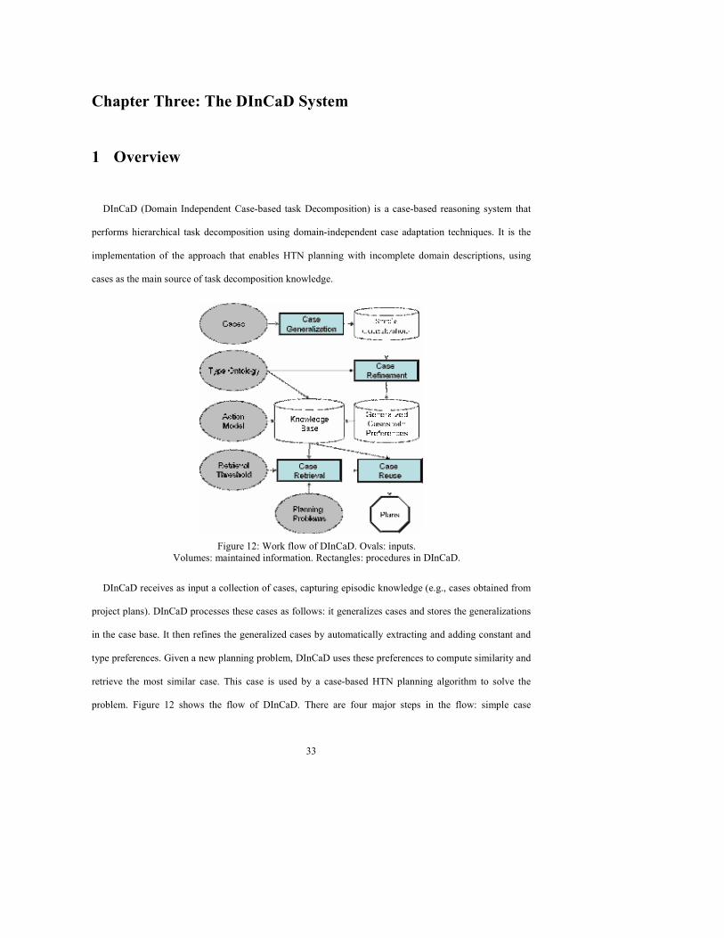
Figure 12: Work flow of DInCaD. Ovals: inputs.
Volumes: maintained information. Rectangles: procedures in DInCaD.
DInCaD receives as input a collection of cases, capturing episodic knowledge (e.g., cases obtained from
project plans). DInCaD processes these cases as follows: it generalizes cases and stores the generalizations
in the case base. It then refines the generalized cases by automatically extracting and adding constant and
type preferences. Given a new planning problem, DInCaD uses these preferences to compute similarity and
retrieve the most similar case. This case is used by a case-based HTN planning algorithm to solve the
problem. Figure 12 shows the flow of DInCaD. There are four major steps in the flow: simple case
Page 34
34
generalization, case refinement, case retrieval, and case reuse. Each step is represented with a rectangle in
Figure 12. Ovals represent inputs that are required by each step. Volumes represent information maintained
by DInCaD. First cases are received as input. These cases are generalized with a simple generalization
process (Section 1.1 in this chapter). Generalized cases are refined by adding preferences to them (Section
1.2 in this chapter). These refined generalized cases, together with the action model and the type ontology
form the domain description used by DInCaD. Given a new problem, DInCaD retrieves generalized cases
which are then reused to solve the new problem. In this chapter, the retrieval procedure is explained in
Section 1.3, and the reuse procedure in Section 1.4.
1.1 Simple Case Generalization
A generalized case gC = (h’, Q’, Pref, ST’) is called a simple generalization of a case C = (h, Q, ST), if
gC is obtained by replacing each constant x in C with a unique variable ?x, such that the type v of x is
known. In this situation, a condition ?x type: v is also added to Q’. For constants in C whose types are
unknown, they are kept as constants in gC. In addition, a condition different ?x ?y is added in Q’ for each
two different variables ?x and ?y of the same type. Table 4 shows a case and its corresponding simple
generalization. The case C accomplishes a task of delivering a piece of equipment, e3, between two offices,
o7 and o9. The task is accomplished by a compound subtask, which is to contract a delivery company, dc2,
for the delivery. The generalization gC replaces constants with variables and adds the condition different
?o7 ?o9.
C gC
Head:
deliver e3 o7 o9
Conditions:
e3 type: Equipment
o7 type: Office
o9 type: Office
dc2 type: Delivery Company
at e3 o7
Subtasks:
contract dc2 e3 o7 o9
Head:
deliver ?e3 ?o7 ?o9
Conditions:
?e3 type: Equipment
?o7 type: Office
?o9 type: Office
?dc2 type: Delivery Company
at ?e3 ?07
different ?o7 ?o9
Preferences:
Subtasks:
contract ?dc2 ?e3 ?o7 ?o9
Table 4: A case and its simple generalization
Page 35
35
1.2 Preference-Guided Case Refinement
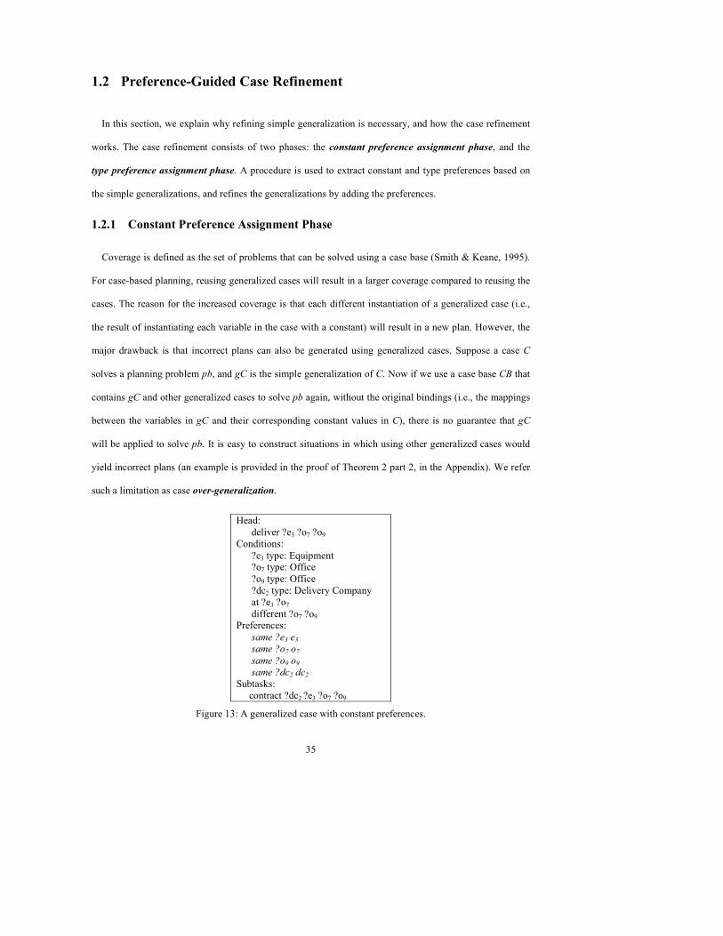
In this section, we explain why refining simple generalization is necessary, and how the case refinement
works. The case refinement consists of two phases: the constant preference assignment phase, and the
type preference assignment phase. A procedure is used to extract constant and type preferences based on
the simple generalizations, and refines the generalizations by adding the preferences.
1.2.1 Constant Preference Assignment Phase
Coverage is defined as the set of problems that can be solved using a case base (Smith & Keane, 1995).
For case-based planning, reusing generalized cases will result in a larger coverage compared to reusing the
cases. The reason for the increased coverage is that each different instantiation of a generalized case (i.e.,
the result of instantiating each variable in the case with a constant) will result in a new plan. However, the
major drawback is that incorrect plans can also be generated using generalized cases. Suppose a case C
solves a planning problem pb, and gC is the simple generalization of C. Now if we use a case base CB that
contains gC and other generalized cases to solve pb again, without the original bindings (i.e., the mappings
between the variables in gC and their corresponding constant values in C), there is no guarantee that gC
will be applied to solve pb. It is easy to construct situations in which using other generalized cases would
yield incorrect plans (an example is provided in the proof of Theorem 2 part 2, in the Appendix). We refer
such a limitation as case over-generalization.
Head:
deliver ?e3 ?o7 ?o9
Conditions:
?e3 type: Equipment
?o7 type: Office
?o9 type: Office
?dc2 type: Delivery Company
at ?e3 ?o7
different ?o7 ?o9
Preferences:
same ?e3 e3
same ?o7 o7
same ?o9 o9
same ?dc2 dc2
Subtasks:
contract ?dc2 ?e3 ?o7 ?o9
Figure 13: A generalized case with constant preferences.
Page 36
36
To address this limitation, constant preferences are added to gC based on the original constants in C. A
new constant preference same ?con con is added for each constant con in C. For example, in the
generalized case shown in Table 4, the following constant preferences are added: same ?e3 e3, same ?o7 o7,
same ?o9 o9 and same ?dc2 dc2. If pb is given as a problem again, gC will have all of its constant
preferences satisfied (since pb has all the constants that are included in the preferences), whereas other
cases will have some constant preferences not satisfied. Therefore, gC will be retrieved according to the
similarity criterion, which we will define in Section 1.3 and applied to solve pb. Figure 13 shows the
generalized case in Table 4, with constant preferences.
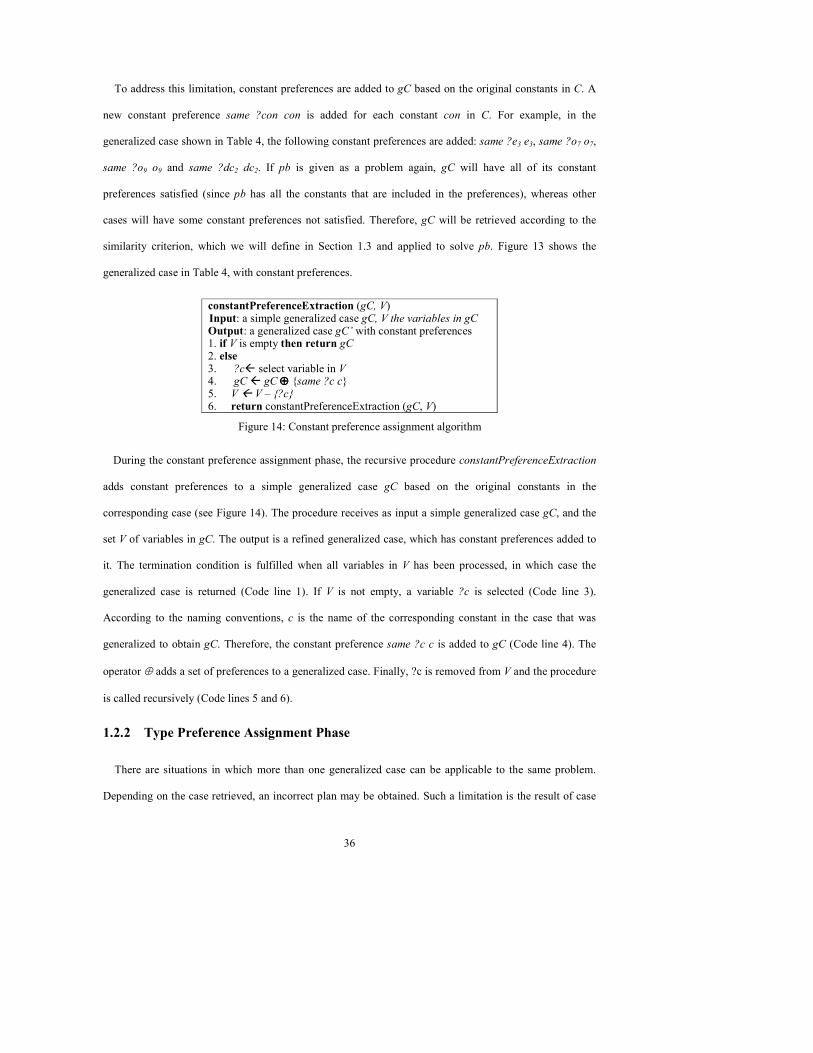
constantPreferenceExtraction (gC, V) Input: a simple generalized case gC, V the variables in gC Output: a generalized case gC’ with constant preferences 1. if V is empty then return gC 2. else 3. ?c select variable in V 4. gC gC ⊕⊕⊕⊕ same ?c c 5. V V – ?c 6. return constantPreferenceExtraction (gC, V)
Figure 14: Constant preference assignment algorithm
During the constant preference assignment phase, the recursive procedure constantPreferenceExtraction
adds constant preferences to a simple generalized case gC based on the original constants in the
corresponding case (see Figure 14). The procedure receives as input a simple generalized case gC, and the
set V of variables in gC. The output is a refined generalized case, which has constant preferences added to
it. The termination condition is fulfilled when all variables in V has been processed, in which case the
generalized case is returned (Code line 1). If V is not empty, a variable ?c is selected (Code line 3).
According to the naming conventions, c is the name of the corresponding constant in the case that was
generalized to obtain gC. Therefore, the constant preference same ?c c is added to gC (Code line 4). The
operator ⊕ adds a set of preferences to a generalized case. Finally, ?c is removed from V and the procedure
is called recursively (Code lines 5 and 6).
1.2.2 Type Preference Assignment Phase
There are situations in which more than one generalized case can be applicable to the same problem.
Depending on the case retrieved, an incorrect plan may be obtained. Such a limitation is the result of case
Page 37
37
over-generalization. As an example, consider the two generalized cases in Table 5. The generalized case
gC1 achieves a task to deliver a liquid, ?e1, between two locations, ?d1 and ?d3, using a truck with a normal
tanker, ?t5. The generalized case gC2 achieves a task to deliver a perishable liquid, ?e4, between two
locations, ?d6 and ?d7, using a truck with a refrigerated tanker, ?t1. Consider a type ontology Ω defining the
following relations: RefrigTanker isa Tanker, RegularTanker isa Tanker, and PerishableLiquid isa Liquid.
Suppose that a new problem is given, where a perishable liquid has to be delivered between two locations,
and that two trucks are available, one is with a refrigerated tanker and another is with a regular tanker. Then
both cases are applicable to the problem. However, reusing gC1 may yield an incorrect plan if it picks the
truck with a regular tanker to deliver the perishable liquid, because if a regular tanker is used to transport a
perishable liquid such as milk, the liquid will decay. In this situation, case over-generalization occurs due to
what we call a type conflict between gC1 and gC2, with respect to the type ontology.
gC1 gC2
Head:
deliver ?e1 ?d1 ?d3
Conditions:
?t5 type: Tanker
?e1 type: Liquid
?d1 type: Depot
?d3 type: Depot
at ?e1 ?d1
at ?t5 ?d1
different ?d1 ?d3
Preferences:
Subtasks:
!load ?e1 ?t5 ?d1
!drive ?t5 ?d1 ?d3
!unload ?e1 ?t5 ?d3
Head:
deliver ?e4 ?d6 ?d7
Conditions:
?t1 type: RefrigTanker
?e4 type: PerishableLiquid
?d6 type: Depot
?d7 type: Depot
at ?e4 ?d6
at ?t1 ?d6
different ?d6 ?d7
Preferences:
Subtasks:
!load ?e4 ?t1 ?d6
!drive ?t1 ?d6 ?d7 !unload ?e4 ?t1 ?d7
Table 5: Two generalized cases that may result in case over-generalization
Two generalized cases gC1 and gC2 are in type conflict relative to Ω if the followings are met: (1) The
heads, h1’ of gC1 and h2’ of gC2, match (i.e., match(h1’, h2’)), and (2) There are at least two variables, ?v1 in
gC1 and ?v2 in gC2, in type conflict relative to Ω. That is, the type of ?v1 is a descendant of the type of ?v2
relative to Ω, or vice versa. We say that a case base CB is in type conflict relative to a type ontology Ω if
there is at least a pair of generalized cases in CB that are in type conflict relative to Ω.
Comment [kex1]: Forget using sub θ here
Page 38
38
To reduce case over-generalization caused by type conflict, type preferences are added to generalized
cases. In the example, the type preferences not ?t5 type: RefrigTanker and not ?e1 type: PerishableLiquid
are added to gC1. The case gC2 will have no type preferences because its conditions are more specific than
those of gC1. Our purpose is to select the most specific generalized case relative to the type ontology Ω. As
we will see in the next section, gC2 will have a similarity higher than gC1 because of the type preferences
added. Table 6 shows gC1 and gC2 after type preferences are added.
gC1 gC2
Head:
deliver ?e1 ?d1 ?d3
Conditions:
?t5 type: Tanker
?e1 type: Liquid
?d1 type: Depot
?d3 type: Depot
at ?e1 ?d1
at ?t5 ?d1
different ?d1 ?d3
Preferences:
not ?t5 type: RefrigTanker
not ?e1 type: PerishableLiquid
Subtasks:
!load ?e1 ?t5 ?d1
!drive ?t5 ?d1 ?d3
!unload ?e1 ?t5 ?d3
Head:
deliver ?e4 ?d6 ?d7
Conditions:
?t1 type: RefrigTanker
?e4 type: PerishableLiquid
?d6 type: Depot
?d7 type: Depot
at ?e4 ?d6
at ?t1 ?d6
different ?d6 ?d7
Preferences:
Subtasks:
!load ?e4 ?t1 ?d6
!drive ?t1 ?d6 ?d7 !unload ?e4 ?t1 ?d7
Table 6: Two generalized cases that may result in case over-generalization
During the type preference assignment phase, the recursive procedure typePreferenceExtraction detects
type conflicts between generalized cases, and eliminates type conflicts by adding type preferences into
generalized cases. Figure 15 shows the pseudo-code of the procedure. The procedure receives as input a
generalized case gC refined with constant preferences, a case base CB without type conflicts relative to a
type ontology Ω, and the currently refined case base CB’, which initially is empty. The procedure returns
the case base CB’ obtained by eliminating the type conflicts in the case base CB ∪ gC. The termination
condition is fulfilled when CB is empty, in which case CB’ ∪ gC is returned (Code line 1). If CB is not
empty, a case gCi in CB is selected and eliminated from CB (Code lines 3-4). The head of gCi is assigned to
ti, and the head of gC is assigned to t (Code line 5). The procedure checks if the heads match (Code line 6).
The extractPreference procedure checks if there is a type conflict between every pair of variables from gC
and gCi. The procedure takes as input two generalized cases and the type ontology Ω. It returns two sets of
Page 39
39
type preferences, Pref and Prefi, which eliminate the type conflicts between gC and gCi, respectively (Code
line 7). The sets of preferences are empty if gC and gCi do not have type conflict. The operation ⊕ adds a
set of preferences to a generalized case. If the set is empty, ⊕ leaves the case unmodified (Code lines 8-9).
Finally, the case gCi is added to the case base CB’ and the procedure is called recursively (Code lines 10-
11).
typePreferenceExtraction(gC, CB, CB’, Ω)
Input: A generalized case gC with preferences, a case base CB without
type conflicts relative to a type ontology Ω, a case base CB’
which is initially empty.
Output: a case base CB’ obtained by eliminating the type conflicts in the
case base CB ∪ gC
1. if CB is empty then return CB’ ∪ gC
2. else
3. gCi select a case in CB
4. CB CB – gCi
5. tihead(gCi); t head(gC)
6. if match(ti, t) then
7. (Prefi, Pref) extractPreference(gCi, gC, Ω)
8. gCi gCi ⊕⊕⊕⊕ Prefi
9. gC gC ⊕⊕⊕⊕ Pref
10. CB’ CB’ ∪ gCi
11. return typePreferenceExtraction(gC, CB, CB’ Ω)
Figure 15: Type preference assignment algorithm
1.2.3 Case Base Maintenance
In (Wilson & Leake 2001), case base maintenance is defined as to implement “policies for revising the
organization or contents (representation, domain content, accounting information, or implementation) of
the case base in order to facilitate future reasoning for a particular set of performance objectives”. In that
paper, a framework for classifying case base maintenance policies was also proposed, consisting of four
maintenance steps: data collection, triggering, operation types, and execution. Data collection is to gather
information that could help determine whether maintenance should be performed. The information can be
collected from individual cases, part of or the whole case base, or the behavior of a CBR system.
Triggering takes the collected data as input, and makes the decision on whether maintenance is necessary.
Operation types provide a collection of maintenance operations. Eventually, during the execution step, the
selected maintenance operations will be applied to the case base.
Page 40
40
As for each maintenance step, various dimensions can be applied to define different maintenance
approaches. For example, data collection can be classified by three dimensions: type of data, timing, and
integration. Types of data regarding whether maintenance should be performed are defined. There could be
no data acquired during data collection, which is referred as a non-introspective maintenance policy.
Introspective policies include using a single snapshot (synchronic) or using a sequence of snapshots
(diachronic) of a case base. Data collection can be performed on different timing basis (i.e., periodic,
conditional or Ad Hoc), and it can be done with two integrations: on-line or off-line.
Case Base Maintenance Dimensions DInCaD Case Refinement
Type of Data Introspective (Synchronic)
Timing Periodic
Data Collection
Integration Off-line
Timing Conditional Triggering
Integration Off-line
Target Type Domain Contents Operation Type
Revision Level Knowledge Level
Timing Conditional Execution
Integration Off-line
Table 7: Case base maintenance dimensions of case refinement in DInCaD
For DInCaD, case base maintenance happens during the case refinement procedure. We use the
framework explained above to classify the maintenance performed during case refinement. Table 7 gives a
complete illustration of the dimensions for each maintenance step. As for the data collection, the type of
collected data is synchronic. A snapshot of a generalized case and its corresponding case is taken during
constant preference assignment, for determining if any constant preferences should be generated; a
snapshot of each two generalized cases is taken during type preference assignment, for determining if any
type preferences should be generated. The timing of data collection is periodic, because it happens before
case retrieval: either when generalized cases are captured from the input cases, or when generalized cases
are compared against each other. The integration of data collection is off-line, because the refinement could
happen before any reasoning and planning activities. As for the triggering, the timing is conditional. The
refinement is triggered if corresponding variables and constants are found, or if type conflicts between
generalized cases are detected. The triggering happens before reasoning/planning, and therefore the
integration is off-line. As for the operation type, the target type is domain contents: as the major domain
knowledge, the generalized cases are refined with preferences. The revision level is at the knowledge level,
given that new knowledge (preferences) about the target domain is learnt. As for the execution, the timing
Page 41
41
is conditional because refinement is made when: a pair of corresponding variable and constant is found and
a constant preference is generated, or a type conflict is detected and a type preference is generated. The
integration is off-line as well, because the execution of the refinement happens before any reasoning or
planning activities.
1.3 Generalized Case Retrieval
Generalized cases are retrieved according to their similarities to the problem being solved. We define a
similarity criterion that is biased towards selecting the most specific generalized case (i.e., the one has the
most satisfied preferences). We expect that a case satisfying more preferences will more likely reduce case
over-generalization. Our theoretical and experimental evaluation will support this claim. The following is
the formula of the similarity criterion:
sim(gC, pb) = appl*( w1 * stp + w2 * scp) (Formula 1)
In the formula, gC = (h, Q, Pref, ST) is a generalized case, and pb = (t, S) is a task-state pair (i.e., the
current task being decomposed and the current state). The formula returns the similarity of gC to pb. The
similarity has a fixed range between 0 and 1. The parameters in the formula have the following properties:
• The applicability value appl can take a value of either 0 or 1. It takes a value of 1 if gC is
applicable to pb, and a value of 0 otherwise.
• The value of stp is obtained by dividing the number of satisfied type preferences by the total
number of type preferences in gC. If gC has no type preferences, stp is assigned a value of 1.
The reason for this is that very specific generalized cases may not have type preferences.
• The value of scp is obtained by dividing the number of satisfied constant preferences by the
total number of constant preferences in gC. Generalized cases always contain constant
preferences.
• The weights w1 and w2 satisfy that 0 ≤ wi ≤ 1 (i = 1,2) and w1 + w2 = 1.
During case retrieval, a threshold α will be set. The value of the threshold is in the same range as the
similarity defined in Formula 1. Given a problem pb, similarity of each generalized case are computed.
Among those cases, a generalized case gC with the highest similarity such that sim(gC, pb) ≥ α will be
retrieved. If more than one generalized case has the same highest similarity, one case is chosen randomly.
If there is no gC such that sim(gC, pb) ≥ α, then no case is retrieved. We called this case retrieval criterion
the αααα-retrieval criterion. The retrieval criterion by itself does not guarantee that reusing every retrieved
Page 42
42
case will generate a correct plan to the problem. However, taking advantage of the preceding case
refinements, the likelihood of solving the problem correctly with the retrieved case is high. The results
from the empirical evaluations discussed in Section 3 support the claim.
With the case retrieval in DInCaD, the limitation of case over-generalization can be solved. As an
example, continuing with Table 6 in Section 1.2.2, the type preferences not ?t5 type: RefrigTanker and not
?e1 type: PerishableLiquid are added to gC1. Suppose that a new problem, which has two trucks, one with a
regular tanker and one with a refrigerated tanker, is given. In this situation there are four possibilities: ?t5
can be instantiated to (1) the regular or (2) the refrigerated tanker, and ?t1 can be instantiated to (3) the
regular or (4) the refrigerated tanker. In the first situation, gC1 will only satisfy one of its two type
preferences (i.e., not ?t5 type: RefrigTanker) and therefore stp = 0.5. In the second situation, gC1 will satisfy
none of its two type preferences and therefore stp = 0. In the third situation, gC2 will not satisfy the
conditions: ?t1 type: RefrigTanker and therefore appl = 0. Finally, in the fourth situation, gC2 will satisfy all
of its conditions and since it has no type preferences stp = 1. Assuming that the constants in the new
problem does not satisfy the original bindings from any of the two cases (i.e., scp = 0 for both gC1 and
gC2). Therefore, the fourth situation yields the highest similarity to the problem, resulting in retrieving a
generalized case (i.e., gC2) that yields a correct plan.
1.4 Generalized Case Reuse
Once a generalized case gC = (h, Q, Pref, ST) is retrieved for a task-state pair (t, S), it is reused in a
standard HTN planning fashion. If θ is a substitution fulfilling the applicability requirement of gC, the task
t is decomposed with the subtasks STθ. The task decomposition process continues recursively with the
subtasks until primitive tasks are obtained.
Page 43
43
CaseReuse((T, S), DK, α) Input: A planning problem consisting of a set of tasks T, a state S, domain knowledge DK
(containing an action model, a possibly empty task model, and generalized cases), and a
retrieval threshold α Output: A plan for the problem
1. if T = nil then return nil endif
2. t = the first task in T
3. U = the remaining tasks in T
4. if t is primitive and there is an operator O applicable to t, then
5. Apply O and get a simple plan p for t
6. P = CaseReuse((U, result(S, p)), DK, α) 7. if P = FAIL then return FAIL endif
8. return Suffix(p, P)
9. else if t is compound and there are methods applicable to t, then
10. randomly choose one of the applicable method, and get a reduction R of t
11. return CaseReuse((Prefix(R, U), S), DK, α) 12. else if t is compound and a generalized case gC can be retrieved according to the retrieval
criterion then
13. retrieve gC, and get a reduction R of t
14. return CaseReuse((Prefix(R, U), S), DK, α) 15. else
16. return FAIL
17. endif
end CaseReuse
Figure 16: Case reuse planning algorithm
Figure 16 shows the HTN planning algorithm CaseReuse, used by DInCaD. The recursive algorithm
receives as input a planning problem consisting of a set of tasks T, a state S, domain knowledge DK (it
contains an action model, a possibly empty task model, and generalized cases), and a retrieval threshold α.
It returns a plan, if any, solving the problem. CaseReuse first checks a termination condition. It terminates
if there is no task to decompose Line 1 in Figure 16). If T has at least one task, t is assigned the first task in
T (Line 2) and U the remaining (Line 3). If t is a primitive task and there is an operator in DK applicable to
t (Line 4), CaseReuse chooses the applicable operator, and uses the operator to get a simple plan p for t
(Line 5). CaseReuse is then recursively called to solve U (Line 6). If CaseReuse returns a failure for U,
then there is no plan for T. CaseReuse will return the failure and terminate (Line 7). The procedure
Suffix(p, P) appends a simple plan p at the end of a plan P. If CaseReuse returns a plan P for U, p will be
appended at the end of P (Line 8). If t is compound, and there are methods in DK applicable to t (Line 9),
CaseReuse randomly chooses one applicable method, and gets a reduction R of t (Line 10). The procedure
Prefix(R, U) appends a reduction R before a set of tasks U. CaseReuse is then recursively called to return a
plan for Prefix(R, U) (Line 11). If t is compound and there are generalized cases in DK applicable to t
Page 44
44
(Code line 12), then CaseReuse chooses an applicable case with the highest similarity to t, relative to S, and
gets a reduction R of t (Line 13). CaseReuse is then recursively called to return a plan for Prefix(R, U)
(Code line 14). Otherwise, CaseReuse returns a failure and terminates (Lines 15 to 17).
2 Properties of DInCaD
In this section, we discuss the properties of DInCaD. We assume that the action model (i.e., the complete
set of operators) is available, which is necessary for being able to state the correctness of a plan. For our
analysis, we will consider the following four case bases and their corresponding case retrieval procedures:
• CB-C, the case base consisting of the original input cases. If a case C is applicable to a task t,
relative to a state S, the similarity of C is set to 1; otherwise, the similarity is set to 0. Recall that a
case is applicable if for each of its positive conditions q, there is an atom q’ in the current state
such that q = q’; and for each of its negative conditions, not(q), there is no atom q’ in the current
state such that q = q’.
• CB-S, the case base obtained with the simple case generalization procedure applied to the cases in
CB-C. If a case C is applicable to a task t relative to a state S, the similarity of C is set to 1;
otherwise, the similarity is set to 0. Recall that a generalized case is applicable if there is a
substitution θ such that for each of its positive conditions q there is an atom q’ in the current state
satisfying qθ = q’; and for each of its negative conditions, not(q), there is no atom q’ in the current
state satisfying qθ = q’.
• CB-CP, the case base obtained with the constantPreferenceExtraction procedure applied to the
cases in CB-S, relative to the corresponding cases in CB-C. Case similarity is computed using
Formula 1, assuming stp = 0.
• CB-CTP, the case base obtained with typePreferenceExtraction procedure applied to the cases in
CB-CP, according to a type ontology Ω. Case similarity is computed using Formula 1.
We will state the theoretical properties of DInCaD without proofs. The proofs of these statements can be
found in the Appendix.
Page 45
45
Definition (Correct Plan). Suppose (T, S, D) is a planning problem, where T = (t1t2…tk) is a task list, S is a
state, and D is a domain description. Suppose that P = (h1h2…hn) is a plan. Then we say that P is a correct
plan for T relative to S in D, if any of the following is true:
1. T and P are both empty, (i.e., k = 0 and n = 0);
2. t1 is a primitive task, h1 is a simple plan for t1, (h2…hn) is a correct plan for (t2…tk) relative to
result(S, h1) in D;
3. t1 is a compound task, and there is a reduction (r1…rj) of t1 in D such that P is a correct plan for
(r1…rjt2…tk) relative to S.
The HTN planning algorithm CaseReuse follows the same kind of decomposition process as in the
SHOP system but extended to use generalized cases. This implies that CaseReuse must also consider the
generalized cases’ preferences. As explained in Section 5.3, cases are ranked according to the preferences.
We refer to the planning algorithm in SHOP as SHOP(T, S, D), in which T is the task being solved, S is the
state, and D is the domain description.
Lemma 1. If SHOP(T, S, D) returns a plan P, then P is a correct plan.
We denote the knowledge bases used for plan generation as I∪CB, where I is an incomplete domain
description containing a set of operators and a subset (possibly empty) of the methods for the target domain
and CB is a case base. Since we do not know a complete domain description that models the planning
domain, we formulate properties based on any domain description D that is consistent with I∪CB
according to the following definition.
Definition (Consistency). If I is an incomplete domain description and CB is a case base, then a domain
description D is consistent with the knowledge base I∪CB iff:
1. Every method and operator in I is an instance of a method or operator in D,
2. For every case C = (h, Q, ST) in CB, there is a method M = (h’, Q’, ST’) in D such that h, Q, and
ST are instances of h’, Q’ and ST’, respectively.
Page 46
46
3. For every generalized case gC = (h, Q, Pref, ST) in CB, there is a method M = (h’, Q’, ST’) in D
such that h, Q, and ST are instances of h’, Q’ and ST’, respectively.
Preferences are ignored in numeral 3 of the definition of consistency, because they represent conditions that
are desired but not required. The following lemma states that any plan generated by the CaseReuse
procedure with I∪CB-C can be reconstructed by SHOP using any planning domain theory D consistent
with I∪CB-C.
Lemma 2. If CaseReuse(T, S, I∪CB-C) returns a plan P, then for any domain description D that is
consistent with I∪CB-C, SHOP(T, S, D) returns P.
The next theorem states that plans generated by I∪CB-C are correct in any consistent domain
description D, but that this property does not hold for I∪CB-S, I∪CB-CP, or I∪CB-CTP.
Theorem 1. The following statements are true:
1. Plans obtained by CaseReuse(T, S, I∪CB-C) are correct in every consistent domain description D.
2. There exists a domain description D consistent with I∪CB-C such that plans obtained with
CaseReuse(T, S, I∪CB-S), CaseReuse(T, S, I∪CB-CP), or CaseReuse(T, S, I∪CB-CTP) are not correct
in D.
The previous result indicates that we cannot guarantee that plan generation with I∪CB-S, I∪CB-CP, and
I∪CB-CTP is sound. However, we found a restricted form of soundness for I∪CB-CP and I∪CB-CTP.
Before stating the result, let us consider the following definition. Let PS = (pb1, sol1), (pb2, sol2), …, (pbn,
soln) be the problem-solution set used to generate CB-C. Each pbi is a task-state pair (Ti, Si) and each soli
is a plan to pbi.
Page 47
47
Definition (Relative Soundness). A knowledge base I∪CB is sound relative to PS iff whenever a problem
pbi in PS is given, the plan generated by using I∪CB is correct in any domain description D consistent with
I∪CB-C.
The rationale behind this definition is that at the very least the case-based planner should find correct
plans for the problem-solution pairs previously acquired as cases.
The notion of soundness relative to PS does not imply that the plan obtained by using CB must be soli
when the problem pbi is given again. Suppose that Ci is the case obtained from (pbi, soli), and that when pbi
is given again as a problem, a different case Ck is retrieved. Under the assumptions, Ci must imply Ck.
Definition (Case Implies Case). Given a retrieval criterion, a case Ci implies a case Ck if whenever Ci can
be retrieved, Ck can also be retrieved.
C1 C2
Head:
deliver e3 o7 o9
Conditions:
1. e3 type: Equipment
2. o7 type: Office
3. o9 type: Office
4. dc2 type: Delivery Company
5. at e3 o7
Subtasks:
contract dc2 e3 o7 o9
Head:
deliver e3 o7 o9
Conditions:
1. e3 type: Equipment
2. o7 type: Location
3. o9 type: Office
4. dc2 type: Delivery Company
5. at e3 o7
Subtasks:
contract dc2 e3 o7 o9
Table 8: Example of case implication. Case C1 implies case C2.
Trivially, a case implies itself according to this definition. Table 8 shows an example of a case C1
implying a non-identical case C2. The heads and conditions 1, 3, 4 and 5 are identical. Condition 2 is not
identical but if we assume that type Office is a subtype of type Location, then if condition 2 of C1 is
satisfied in a state S, condition 2 of C2 is also satisfied in S. The following lemma establishes sufficient
conditions under which case Ci implies a case Ck.
Lemma 3. Under the α-retrieval criterion, if a case Ci implies a case Ck, then the following conditions are
true:
Page 48
48
1. The head of Ci and Ck are identical,
2. There is a one-to-one mapping from the conditions in Ci to the conditions in Ck, with which either
of the following is true:
(i) Each condition q in Ck is also a condition in Ci,
(ii) If a condition of the form v1 type: t1 occurs in Ck but not in Ci, then there must be a condition
of the form v1 type: t2 in Ci, such that t2 is a subtype of t1 in the type ontology Ω.
The following theorem states the relative soundness of I∪CB-CP and I∪CB-CTP.
Theorem 2. Let PS be the problem-solution set used to generate CB-C. The following statements are true:
1. I∪CB-C is sound relative to PS.
2. I∪CB-S is not sound relative to PS.
3. I∪CB-CP is sound relative to PS.
4. I∪CB-CTP is sound relative to PS.
The last issue is the coverage of the case bases (Smyth & Keane, 1995). We extend the traditional notion
of the coverage of a case base to the coverage of a knowledge base I∪CB.
Definition (Coverage). Suppose I is an incomplete domain description, CB is a case base. The coverage of
the knowledge base I∪CB is defined as:
Coverage(I∪CB) = pb: pb is a solvable planning problem that can be solved by using I∪CB
The definition of coverage does not indicate if the plan found for pb is correct or not. It just indicates if a
plan can be found or not. With the definition of coverage, we state the following theorem:
Theorem 3. The following statements are true:
1. Coverage(I∪CB-C) ⊆ Coverage(I∪CB-S)
2. Coverage(I∪CB-S) = Coverage(I∪CB-CP) = Coverage(I∪CB-CTP)
Page 49
49
From the analysis, we conclude that, among the three case bases containing generalized cases, CB-CTP and
CB-CP have the largest coverage while preserving soundness relative to the problem-solution set.
However, as we will show in the experimental evaluation, CB-CTP has the best performance in terms of
reducing case over-generalization.
3 Empirical Evaluation
The analysis of the properties of DInCaD in the previous section shows that using the case bases CB-
CTP and CB-CP will result in the same coverage, and that they are both sound relative to the input
problem-solution set PS. The analysis also shows that although using the case base CB-S will result in the
same coverage, CB-S is not sound relative to PS. We believe that the type and constant preferences
represented in CB-CTP should result in a reduction in case over-generalization compared to CB-CP and
CB-S. To test this claim, we used two evaluation methods, the Receiver Operating Characteristic (ROC)
and Precision-Recall. Later in this section, we will explain how these methods measure the reduction in
case over-generalization. We also conducted experiments evaluating the coverage as a function of the
number of input cases.
3.1 Test Domains
For our experiments we used variants of the following three domains: UM Translog, Process Planning,
and Scheduling domain. All three domains have in common that they are naturally modeled hierarchically.
The UM Translog domain was used to demonstrate the capabilities of the HTN planner UMCP (Erol et al.,
1994). The Process Planning domain indicates how to manufacture mechanical workpieces. The relation
between the components of a workpiece is hierarchical with some areas being sub-areas of other larger
areas. The scheduling domain was defined hierarchically in the SHOP system for the International Planning
Competition. The complete domain description of these domains can be downloaded from
http://www.cse.lehigh.edu/~munoz/projects/DinCaD/, as well as random problem generators that we
implemented for these domains.
Page 50
50
We implemented a variant of the UM Translog domain (Andrews, 1995). In this domain, trucks and
airplanes are used to transport packages between locations in different sites. A type ontology of vehicles
and packages is defined so that vehicles can only deliver compatible packages. For example, medium
trucks transport medium or small packages, but not large packages. We constructed problems following
two possible configurations. Both configurations share the following information in the initial state:
• 5 cities, each having 4 transport locations (3 normal locations and 1 airport);
• 20 trucks, each of which is initially located in a random city, and randomly categorized into one of
the 4 truck types;
• 4 airplanes, each of which is initially located in a random airport, and randomly categorized into
one of the 4 airplane types,
• and several packages at various locations.
The configurations differ in that the first one has a single task relocating one of the packages, whereas the
second one requires to relocate two packages. We performed evaluations for each configuration.
We also implemented an HTN version of the Process Planning domain reported in (Muñoz-Avila &
Weberskirch, 1996). In this domain, plans for manufacturing rotary symmetrical workpieces are generated.
These plans must consider inter-relations between various processing areas of the workpieces, and
available manufacturing tools. For example, one processing area of a workpiece may be first processed by a
cutting tool, and then processed by a drilling tool; while another processing area of the same workpiece has
to be processed by a scope tool. Specifically, a planning problem in the domain consists of: 1 workpiece
contains a maximum of 26 processing areas, 12 manufacturing tools that are randomly categorized into 7
tool types. The processing areas are determined by the geometry of the workpiece. Therefore, the challenge
in the process planning domain is that an intrinsic ordering is required to process these areas because of the
geometry of the workpiece. One characteristic that researchers have pointed out about process planning is
that the whole process is too complex to be performed automatically (e.g., Kambhampati et al., 1995). For
this reason, Muñoz-Avila and Weberskirch propose an interactive system (Muñoz-Avila & Weberskirch,
1996). The system automatically process part of the workpiece. Then, the user manually indicates how to
process other part of the workpiece. Then the system takes control automatically processes other part of the
Page 51
51
workpiece, and so forth. This interaction goes on until the whole workpiece is processed. In our
experiments, we simulate the first step of this interactive process, in which the system (DInCaD) generates
plans for manufacturing part of a workpiece. In particular, DInCaD reuses a case that is capable of
manufacturing at least three processing areas from a given workpiece. Table 9 column (a) shows an
example of a method in this domain. The task is to manufacture a workpiece ?wp. The method picks a
processing area ?part that is rotary and can be processed. It also checks that the ?wp can be mounted from a
part ?part1 to process ?part. It finally checks that there is a processing tool ?tool that can be used to process
?part. If all these conditions are met, the processing task is decomposed in two subtasks. A primitive task
processing ?part with ?tool, and a second (compound) task processing ?wp. The latter acts a s a recursive
call to process other parts of ?wp.
(a) Method in Process Planning (b) Method in Scheduling domain
Head:
manufacture ?wp
Conditions:
processingArea ?part
canProcess ?part
rotary ?part
mountable ?wp ?part1 ?part
tool ?tool
compatible ?part ?tool
Subtasks:
!process ?part ?tool ?wp
manufacture ?wp
Head:
shape ?part cylindrical
Conditions:
not scheduled ?part
type ?mach Lathe
not busy ?mach
temperature ?part cold
Subtasks:
!mount ?part ?mach
!surface-condition ?part rough
!shape ?part cylindrical
!scheduled ?part
Table 9: Example of a method in the process planning domain (a)
and the scheduling domain (b).
The third domain we use is the Scheduling domain. This is a domain from the International AI planning
competition. The reason why we choose this domain is that it is hierarchical and used by the planner SHOP
during the competition. In the Scheduling domain, a collection of pieces and a collection of machines are
given, and the goal is to accomplish a sequence of steps machining the pieces, taking into account the
constraints for the machines. In our experiments, each planning problems contained 3 machining tasks. The
challenge in the scheduling domain is that in order to machine different parts, the characteristics of various
machines have to be consider. For example, if we need to change both the color and the surface condition
of a part, we may need to first use a lathe machine to change the surface condition, and then use a spray
machine to paint it. However, we cannot paint the part first and change the surface because the lathe
Page 52
52
machine removes the paint. Table 9 column (b) shows an example of a method in the scheduling domain.
The task is a single machining step, which is to shape ?part into a cylindrical form. The method requires
?part not to be scheduled, a machine ?mach of type Lathe to be available, ?mach not to be busy, and ?part
to be cold. The subtasks of the method are to mount ?part and ?mach, to make the surface condition of
?part to be rough (this is a side effect of using the Lathe machine), to make ?part cylindrical, and to make
?part scheduled.
3.2 Experimental Setup
In this section, we explain in detail how the experiments were setup and executed. For each test domain,
two sets of problems were randomly generated: the training set and the test set. The problems in the
training set were used to generate cases that DInCaD requires for case-based task decomposition. We used
the SHOP system to simulate users solving the problems. SHOP requires a domain description, including
an action model (operators) and a task model (methods), to generate plans for the. The problems and their
corresponding plans were stored as cases. These cases were used by DInCaD as task decomposition
knowledge. To solve the problems in the test set, DInCaD does not need methods, but requires cases as task
decomposition knowledge, a type ontology (definitions of types and their relations), and the action model.
UM Translog Process Planning Scheduling Domain
Training
Set
Test
Set
Training
Set
Test
Set
Training
Set
Test
Set
Operators 7 7 6 6 19 19
Types 12 12 22 22 13 13
Type Relations 12 9 20 17 10 9
Axioms 11 4 30 2 4 1
Methods 13 0 5 0 32 0
Cases 0 179 0 212 0 215
Table 10: Summary of the domains
Table 10 shows a summary of the data used in the experiments. Axioms are used to simplify operators
and methods. The same domain description can be defined without axioms, but it would result in
substantially complex operators and methods. The type ontology (types and type relations) are referenced
by axioms. As shown in the table, the operators, type ontology, axioms, and methods were used to capture
cases from the training set; while for solving the problems in the test set, an incomplete domain description
Page 53
53
(less type ontology, fewer axioms and no methods) and cases were used. We now present in detail how the
experiments were conducted:
1. Generating the training set.
a) A training set of planning problems was randomly generated.
b) The complete domain description (i.e., the set of operators, methods, axioms and type ontology)
was used by SHOP to generate a plan for each planning problem in the training set.
c) Each solvable planning problem and the generated plan were used as a problem-solution pair to
create a case. These cases formed the case base CB-C.
2. Filling up the three case bases.
a) The simple generalizations of cases in CB-C formed the case base CB-S.
b) The procedure constantPreferenceExtraction (see Figure 14) was used to refine cases in CB-S by
adding constant preferences. The refined cases formed the case base CB-CP.
c) The procedure typePreferenceExtraction (see Figure 15) was used to refine cases in CB-CP by
adding type preferences. The refined cases formed the case base CB-CTP.
3. Generating the test set.
a) A test set consisting of a new collection of 50 planning problems was generated by the same
random problem generator used in step 1 a).
b) The complete domain description was used to determine how many planning problems in the test
set are solvable.
4. Conducting the tests.
We set thresholds for the similarity criterion in case retrieval. The threshold α was set to various
values in the range of 0 and 1. For each of these values, we ran the following steps and collected the
data. These data were then analyzed to compare the ROC graphs and precision-recall graphs of CB-S,
CB-CP and CB-CTP. We will explain in the next section how we analyze the data.
a) CB-S was used to generate plans for the test set. In Step 12 of the CaseReuse procedure (see
Figure 16), the retrieval criterion randomly selects an applicable case.
b) CB-CP was used to generate plans for the test set. In Step 12 of the CaseReuse procedure, the
retrieval criterion selects the case with the highest similarity that is greater than or equal to α. The similarity criterion used is the same as in Formula 1 (introduced in Section 4.3), with w1 set to 0
and w2 set to 1.
c) CB-CTP was used to generate plans for the test set. In Step 12 of the CaseReuse procedure, the
retrieval criterion selects the case with the highest similarity that is greater than or equal to α. The similarity criterion used is the same as Formula 1, with w1 and w2 set to 0.5.
Page 54
54
3.3 Evaluation Metrics
We use two evaluation metrics: Receiver Operating Characteristic (ROC) and Precision-Recall. Before
explaining these metrics, we first give definitions for the evaluation.
3.3.1 Definitions for Evaluation
According to the retrieval criteria we defined for CB-CTP and CB-CP, the case with the highest
similarity larger than or equal to the threshold is retrieved. Therefore, for every given planning problem, at
most one plan will be generated, namely, the one obtained by reusing the retrieved case. As a result, for a
set of planning problems, we define the following values for CB-CTP and CB-CP:
#(Solvable, CPlan): The number of solvable planning problems for which correct plans are
generated using the case base.
#(Solvable, IncPlan): The number of planning problems that are solvable but for which
incorrect plans are generated using the case base.
#(Solvable, NoPlan): The number of solvable planning problems for which no plans are
generated using the case base.
#(Unsolvable, IncPlan): The number of planning problems that are not solvable but for
which plans are generated (and are therefore incorrect) using the case base.
#(Unsolvable, NoPlan): The number of planning problems that are not solvable and for
which no plans are generated using the case base.
For CB-S, however, the definitions are slightly different. Since all the applicable cases will have a
similarity value of 1, the case that is reused for planning has to be randomly selected among all applicable
cases. Therefore, we have to examine all the plans generated using CB-S instead of examining only one
plan as for CB-CTP and CB-CP. Thus, when DInCaD uses CB-S and generates both correct and incorrect
plans to a solvable planning problem, we define #(Solvable, CPlan) for CB-S as the proportion of the
correct plans, and #(Solvable, IncPlan) as the proportion of the incorrect plans. In other situations, the
definitions remain the same as for CB-CTP and CB-CP.
3.3.2 Receiver Operating Characteristic (ROC)
Receiver Operating Characteristic (ROC) analysis is a classic methodology that provides a visualization
comparing tradeoffs between true positive (TP) and false positive (FP) (Provost & Fawcett, 2001). TP is
defined as the ratio of number of positives that are correctly classified to the total number of positives. FP
Page 55
55
is defined as the ratio of the number of negatives that are incorrectly classified to the total number of
negatives. In our experiments, we used ROC graphs to evaluate the tradeoffs between TP and FP for
solving a set of planning problems (i.e., the test set). In a ROC graph, TP is represented on the Y-axis, and
FP is represented on the X-axis. For any two points in a ROC graph, the one to the northwest is considered
better because it has a higher true positive rate and a lower false positive rate. Similarly, for two curves, the
one to the northwest is better. Thus, if we can measure the TP and FP of CB-S, CB-CP and CB-CTP with
various thresholds, and connect the points to curves, we then will be able to compare the case bases’
performances based on the ROC graph. We interpret the metrics for measuring true positive and false
positive for case-based planning as follows:
TP = #(Solvable, CPlan) / (#(Solvable, CPlan) + #(Solvable, NoPlan) + #(Solvable, IncPlan))
FP = #(Unsolvable, IncPlan) / (#(Unsolvable, IncPlan) + #(Unsolvable, NoPlan))
That is, TP represents the ratio of the number of solvable planning problems for which correct plans are
generated to the total number of solvable planning problems. FP represents the ratio of the number of
planning problems that are not solvable but for which plans are generated to the total number of planning
problems that are not solvable. Both TP and FP have a fixed range from 0 to 1.
In the context of planning, solving a planning problem correctly means either finding a valid plan for a
solvable problem, or recognizing an unsolvable problem. Therefore, when we evaluate the problem-solving
capability of a planning system, both situations should be considered. TP is used to reflect the proportion of
solvable problems that are correctly solved, and FP is used to reflect the proportion of unsolvable problems
that are incorrectly recognized. Therefore, we can use the ROC graph to evaluate the problem-solving
capability of a planning system.
Page 56
56
Figure 17: Using a ROC graph to evaluate case over-generalization reduction. Target
Area: a combination of a relatively high true positive (TP) and a relatively low false
positive (FP). O-C: a combination of a low TP and a low FP. O-G: a combination of a
low TP and a high FP.
Figure 17 illustrates how a ROC graph can be used to evaluate the reduction of case over-generalization.
If cases used for plan generation are too concrete, the chance of such cases being applicable to a planning
problem is slim. Thus, few solvable problems will be solved. Problems that are not solvable most likely
will not have plans neither. Therefore, using cases that are too concrete will result in a low TP and a low
FP, which is represented as the “O-C” area in the figure. On the other hand, if case over-generalization
occurs, reusing generalized cases may generate incorrect plans for both solvable and unsolvable planning
problems. This will result in a low TP and a high FP, which is represented as the “O-G” area in the figure.
Therefore, an ideal situation illustrating a reduction in case over-generalization will be a combination of a
relatively high positive and a relatively low false positive, which is represented as the “Target Area” in the
figure.
3.3.3 Precision-Recall
Precision and recall are commonly used to evaluate information retrieval systems (Salton et al., 1975).
Traditionally, precision is defined as the proportion of relevant documents of all documents retrieved.
Recall is defined as the proportion of retrieved relevant documents of all available relevant documents. In
our experiments, we adapted the original definitions of precision and recall, and defined a variant of the
Precision-Recall relation that is suitable for evaluating case-based planning systems. We present this
relation using a Precision-Recall graph. In a Precision-Recall graph, precision is represented on the Y-axis,
and recall is represented on the X-axis. For any two points in a Precision-Recall graph, the one to the
northeast is considered better because it has a higher precision and a higher recall. Similarly, for two
Page 57
57
curves, the one to the northeast is better. Thus, if we can measure the precision and recall of CB-S, CB-CP
and CB-CTP with various thresholds, and connect the points to curves, we then will be able to evaluate the
case bases’ performance based on the Precision-Recall graph. We interpret the metrics for measuring
precision and recall for case-based planning as follows:
Precision = #(Solvable, CPlan) /
(#(Solvable, CPlan) + #(Solvable, IncPlan) + #(Unsolvable, IncPlan))
Recall = (#(Solvable, CPlan) + #(Solvable, IncPlan)) /
(#(Solvable, CPlan) + #(Solvable, NoPlan) + #(Solvable, IncPlan))
That is, the precision is the ratio of the number of solvable planning problems for which correct plans are
generated to the total number of planning problems for which plans are generated. Recall is defined as the
ratio of the number of solvable planning problems for which plans are generated to the total number of
solvable planning problems. Both precision and recall have a fixed range from 0 to 1.
In the context of planning, we expect to solve as many solvable problems as possible and generate as
many correct plans as possible. Precision is used to reflect the proportion of correct plans that are
generated, and recall is used to reflect the proportion of solvable problems for which plans are generated.
Therefore, we can use the Precision-Recall graph to evaluate the balance between finding correct plans and
solving solvable problems.
Figure 18: Using a Precision-Recall graph to evaluate the reduction in case over-
generalization. Target Area: a combination of a relatively high precision and a
relatively high recall. O-C: a combination of a high precision and a low recall. O-
G: a combination of a high recall and a low precision.
Figure 18 illustrates how a Precision-Recall graph can be used to evaluate the reduction in case over-
generalization. If the cases used for plan generation are too concrete, the chance of such cases being
applicable to a planning problem is slim. Few solvable problems will be solved, but generated plans are
Page 58
58
likely to be correct. Therefore, using cases that are too concrete will result in a high precision but a low
recall, which is represented as the “O-C” area in the figure. On the other hand, if case over-generalization
occurs, reusing generalized cases may increase the number of problems that are solved, but also may
generate more incorrect plans. This will result in a high recall but a low precision, which is represented as
the “O-G” area in the figure. Therefore, an ideal situation illustrating a reduction in case over-
generalization will be a combination of a relatively high precision and a relatively high recall, which is
represented as the “Target Area” in the figure.
3.3.4 Relation between Evaluation Metrics and Soundness-Completeness
Case over-generalization is a significant limitation for case-based planning systems because it may result
in incorrect plans. We conducted experiments to evaluate DInCaD’s performance on reducing this
limitation. The ROC graph is used to evaluate the problem-solving capability of a planning system, either
finding a valid plan for a solvable problem, or recognizing an unsolvable problem. The Precision-Recall
graph is used to measure the balance between finding correct plans and solving solvable problems.
Soundness is a desirable property of a planner by which every solution generated is correct. Therefore, if
a provable sound planner is used to solve problems, the resulting precision is 100%. In our situation,
without foreknowledge of a complete domain description, DInCaD is restricted to soundness relative to the
input problem-solution pairs. Therefore, empirical validation is required to measure the degree of precision.
Recall is related to completeness, which is another desirable property of a planner by which a solution can
be found whenever one actually exists (although incorrect solutions might also be generated). If a complete
planner is given to solve problems, a 100% recall will be obtained. In DInCaD, completeness cannot be
guaranteed and therefore we are required to measure the degree of recall. Obviously, a way to ensure 100%
precision and, therefore, soundness is for a planner not to solve any problem at all. But this will set the
recall value to be 0%, indicating that the planner does not solve any problems at all. This is why we
measure and present in the same figure the co-relation between precision and recall.
Page 59
59
The ROC measure is also related to soundness and completeness. If the planner is sound and complete,
TP will be 100% and FP will be 0%. If the planner is sound but not complete, then TP will be smaller than
100% and FP will still be 0%. If the planner is complete but not sound, then TP will be 100% and FP
maybe larger than 0%. If the planner is neither sound nor complete, then TP will be less than 100% and FP
may be larger than 0%. The ROC measure is looking at planners that are not complete and/or not sound, to
see how their values of TP and FP approximate to the ideal values of 100% and 0%, respectively.
3.4 Results
3.4.1 ROC and Precision-recall
(A)
(B)
Figure 19: Results of the Process Planning domain. (A) single package transportation;
(B) multiple packages transportation
Figure 19 shows the empirical results for the UM Translog domain. Part (A) shows the results of the first
configuration (with single package transportation) as discussed in section 7.1. Part (B) shows the results of
the second configuration (with two packages transportation). In each part, the ROC graph is on the left and
the Precision-Recall graph is on the right.
Page 60
60
In the ROC graph of part A, the curve of CB-CTP is to the northwest of CB-CP’s. The curve of CB-S is
a single point because it is independent of the threshold α. If we use this point as the base line, the curve of
CB-CTP is still northwest to it. The point (0.05, 0.5) in the curve of CB-CTP is the most northwest point in
the graph, which represents the combination of the highest true positive and the lowest false positive.
However, the curve of CB-CP is not always northwest to the curve of CB-S.
In the Precision-Recall graph of part (A), the curve of CB-CTP is northeast of CB-CP’s. For the same
reason we explained, the curve of CB-S is a single point. If we use this point as the base line, the curve of
CB-CTP is still northeast to it. The point (0.81, 0.71) in the curve of CB-CTP is the most northeast point in
the graph, which represents the combination of the highest precision and the highest recall. However, the
curve of CB-CP is not always northeast to the curve of CB-S.
In part (B), the results are in the same patterns as those of part (A). In the ROC graph, the curve of CB-
CTP is always to the northwest of CB-CP’s and CB-S’s. In the Precision-Recall graph, the curve of CB-
CTP is always northeast of CB-CP’s and CB-S’s. A difference with part (A) is that in part (B), the
combination of the highest true positive and the lowest false positive, and the combination of the highest
precision and the highest recall, are both smaller than those in part (A), respectively. The reason is that with
the second configuration, planning problems contain multiple tasks. Thus, solving a planning problem
requires reusing more than one case, and therefore is more restrictive with case applicability.
Figure 20 shows the results of the scheduling domain. Although positioned very close, the curve of CB-
CTP in the ROC graph is still northwest to the curve of CB-CP and the point of CB-S. The point (0, 0.35)
in the curve of CB-CTP is the most northwest point in the graph. In the Precision-Recall graph, the curve of
CB-CTP is northeast to the curve of CB-CTP and the point of CB-S. The point (0.94, 0.96) in the curve of
CB-CTP is the most northeast point, with the highest precision and recall.
Page 61
61
Figure 20: Results of the Scheduling domain
Figure 21 shows the results for the Process Planning domain. In the ROC graph, the curve of CB-CTP is
northwest to the curve of CB-CP and the point of CB-S. The point (0, 0.9) in the curve of CB-CTP is the
most northwest point in the graph, with the highest true positive and the lowest false positive. In the
Precision-Recall graph, the curve of CB-CTP is northeast to the curve of CB-CP and the point of CB-S. The
point (1, 0.98) in the curve of CB-CTP is the most northeast point in the graph, with the highest precision
and recall.
Figure 21: Results of the Process Planning domain
Case over-generalization is a significant limitation for case-based planning systems because it may result
in incorrect plans. We conducted experiments to evaluate DInCaD’s performance on reducing this
limitation. In all the domains, CB-CTP has the best approach to the ideal target area compared to other
case bases for both precision-recall and ROC. We therefore conclude that CB-CTP has the best
performance on reducing case over-generalization among the three evaluated case bases.
Page 62
62
3.4.2 Coverage
Coverage is another important concept for evaluation planning systems. Coverage is defined as the set of
problems that can be solved using a case base (Smyth & Keane, 1995). We extended this traditional notion
of the coverage of a case base to the coverage of a knowledge base in Section 6. To evaluate the relation
between the number of cases contained in the knowledge bases and the number of planning problems
solved, we conducted the experiments with the scheduling domain. We executed 5 runs on the test set,
using 100%, 80%, 60%, 40% and 20% of the cases, respectively. Figure 22 shows the coverage in percent
of the UM Translog domain (left) and the Scheduling domain (right). For both domains, DInCaD achieves
a coverage over 80% with 100 refined generalized cases. With 150 cases, DInCaD achieves and maintains
a steady coverage close or equal to 100%. For the Process Planning domain, as discussed in section 7.1, if
any processing area of a workpiece in a problem can be processed, the problem is considered solvable. For
this reason, DInCaD was able to generate plans for every problem with any non-empty case base, resulting
a 100% coverage.
Figure 22: Coverage of the UM Translog Domain and the Scheduling domain
Page 63
63
Chapter Four: A Practical Application – CaBMA
1 Introduction
1.1 Project Planning
Project planning is a business process for successfully delivering one-of-a kind products and services
under real-world time and resource constraints (PMI, 1999). Project planning involves six activities:
(1) Creating a work breakdown structure,
(2) Identifying/incorporating task dependencies,
(3) Estimating task and project duration,
(4) Identifying, estimating, and allocating resources,
(5) Estimating overall project costs or budget,
(6) Estimating uncertainties and risks associated with tasks, their schedules, and resources.
Figure 23: Snapshot of a WBS on MS ProjectTM
Tools for project planning support the user on each of these phases. For example, MS Project™ allows
user edits to a work breakdown structure (WBS). Figure 23 shows a snapshot of a WBS in MS Project™.
The task distribute-packages is decomposed into four subtasks (Task Name column): Distribute
package100 from Allentown to NYC, Distribute package200 from Bethlehem to Beijing, Distribute
package300 from Easton to Newark, and Distribute package400 from ABE to O'Hare. Some tasks, called
Page 64
64
activities, represent concrete actions. For example, Drive truck47 to Allentown is an activity. Tasks have
assigned resources (Resource Name column). For example, the task Distribute truck47 to Allentown has
two assigned resources: truck47 and Allentown. Finally, tasks have ordering relations among them (the
column with schedules). For example, the task Drive truck47 to Allentown occurs before the task Load
truck47 with package100. More generally, there are three kinds of relations in a WBS:
• Task - subtask relations
• Task - resource assignment relations
• Task- task ordering relations
Thus, creating a WBS also provides information about the six project planning activities.
1.2 CaBMA
We are going to present an implementation of an AI system, CaBMA, built on top of a commercial
project planning tool, MS Project™. CaBMA (for: Case-Based Project Management Assistant) adds a
knowledge layer on top of MS Project™ to assist the user with his project planning tasks. CaBMA reuses
cases containing pieces of project plans when creating new project plans, assisting project managers in the
development of a WBS by using HTN planning techniques. This approach is based on the observation that
WBS has a one-to-one correspondence with the hierarchical task networks (Erol et al., 1994). CaBMA
provides the following functionalities:
• It captures cases from project plans
• It reuses captured cases to refine project plans and generate project plans from the scratch
• It maintains consistency of pieces of a project plan obtained by case reuse
• It refines the cases to cope with inconsistencies resulting from capturing cases over a period of time.
2 Motivation
CaBMA addresses the following issues that we encountered while implementing the idea of case reuse
on top of a commercial project planning tool, MS Project™.
Page 65
65
The first issue was how to populate the case base. Do we assume that domain experts create the cases?
Knowledge acquisition is a problem frequently faced when using intelligent problem-solving techniques in
real-world situations. Over the years, intelligent systems were developed but not used because it was not
feasible to feed such systems with adequate knowledge. CaBMA extracts cases automatically from user
interactions with MS Project™. By doing so, the knowledge acquisition effort becomes transparent to the
user. Cases captured are generalizations of project plans. The main advantage of this generalization is that
it increases the opportunities for reusing the cases.
The second issue results from the automated case capture procedure. Situations arise where multiple
cases may be applicable to the same part of a project plan and any of them is reusable. Thus, a case may not
be reused in the same context from which it was captured. Depending on the domain, reusing a different
case may yield an incorrect solution. In such situations, we say that the case capture procedure is not sound
relative to the captured solutions. These inconsistencies are a result of the generalization procedure during
the case capture. However, if cases are not generalized, a very large case base will be required to obtain an
adequate coverage. CaBMA refines the case base over time. This revision process is performed when
potential conflicts between the new and the existing cases are identified.
The third issue emerged during early trials with CaBMA. We identified a problem that is due to the use
of knowledge-based approaches in interactive environments such as MS Project™. When the user requests
CaBMA to complete parts of a project plan, the system responds by identifying applicable cases and
reusing them. Case applicability is determined based on elements of the current project plan. The problem
may arise if the user later changes some of these elements. An inconsistency occurs when cases previously
reused are no longer applicable. We refer to these inconsistencies as case reuse inconsistencies (Xu &
Muñoz-Avila, 2003). These can be seen as a kind of semantic inconsistencies and are complementary to the
syntactical inconsistencies that MS Project™ can detect, which refer to the over-allocation of resources.
CaBMA keeps track of all modifications being performed to the current project plan. These modifications
include user edits and CaBMA-made changes. Edits that may result in case reuse inconsistencies will
Page 66
66
trigger a propagation process by this component. Any inconsistencies detected are pointed out for the user
in a non-intrusive manner allowing the user to decide at what point he/she wants to deal with them.
3 The CaBMA System
3.1 Overview of the System
CaBMA adds a knowledge layer on top of MS Project™ to assist the user with the project management
tasks, using experience captured from previous project planning episodes. CaBMA consists of three main
components. The first component is Gen+, which captures cases automatically. Gen+ generalizes the cases
from task decompositions in the WBS to increase the re-usability of the cases. However, this may result in
problems due to the generalization process. Gen+ also provides a procedure to refine the cases over time.
The second component is SHOP/CCBR. This component follows a HTN planning paradigm for case reuse.
As user edits may violate applicability conditions of the cases, the third component, the Goal Graph
Component (GGC), detects such inconsistencies and indicates them to the user in an unobtrusive manner.
Figure 14: Work flow of CaBMA
Figure 24 interprets the work flow of CaBMA. First, the user edits a project plan in MS Project™. This
means that the user edits tasks, relations, and the available resources in the WBS. The user selects to store
part or the whole WBS generated. Gen+ stores one or more cases in the case base and may refine existing
cases if necessary. The user can at any time select a task in the WBS and use CaBMA to generate a
Page 67
67
decomposition for that task. SHOP/CCBR is the component of CaBMA that reuses cases to decompose
tasks. As the user edits some parts of the WBS may become inconsistent relative to the reused cases. GGC
keeps track of edits performed by the user and reused cases. GGC also alerts the user of potential
inconsistencies in an unobtrusive manner. In the following sections, we explain each component in detail.
3.2 The Gen+ Component
3.2.1 Capturing Cases with Gen+
Gen+ is the component of CaBMA responsible for capturing cases from existing project plans and
refining the case base. To capture cases, work breakdown structures in previous project plans are treated as
a collection of one-level decompositions, and each of the decomposition is stored as a case by Gen+. In
(Mukammalla & Muñoz-Avila, 2002), the trade-offs between cases containing one-level decompositions
and multiple-level decompositions were studied and compared, and capturing cases with one-level
decompositions was preferred because it “maximize the reusability of the cases” for knowledge-based
project planning. Cases captured by Gen+ are obtained by generalizing the decompositions from the WBSs.
This is because of the same reason as for the DInCaD system – to reduce the number of cases required
during planning. As an example, Table 4 shows an example of how a one-level decomposition from a WBS
of a project plan is captured by Gen+ as a case. The decomposition is to deliver an equipment equip103
between two specific locations: dept107 and office309. Gen+ generates the case from the one-level
decomposition with the following rules:
• Replace each resource item with a unique variable, ?ψ only if the type of the item is known,
• A resource item is not replaced with a variable and is viewed as a constant if its type is unknown,
• For each two different variables, ?x and ?y, of the same type, a constraint: different ?x ?y is
added,
• For each constant, c, and each variable, ?x, a constraint: different ?x c is added.
One-level Decomposition Gen+ Case 1
Task: deliver equip103 dept107 office309
Resources: Deliver_inc equip103
dept107 office309
Task: deliver ?e ?d ?o
Conditions: deliverCompany ?fd
equipment ?e
depot ?d office ?o
Page 68
68
Subtasks: contract Deliver_inc equip103 dept107 office309
Subtasks: contract ?fd ?e ?d ?o
Table 4: A one-level decomposition and the corresponding case captured by Gen+.
3.2.2 Refining Cases with Gen+
Cases captured by Gen+ are reused to generate a work breakdown structure for a new project. It was
found that reusing the cases may yield incorrect solutions in some situations. For an example of such
situations, continuing with the example shown in Table 4, suppose now that a new case is captured by
Gen+ from another one-level decomposition (shown in Table 5). The main difference between the
decompositions is that the equipment is delivered in two steps in the latter one: first Deliver Incorporated is
once again contracted to deliver the equipment to depot55, and then one of the company’s own truck is
used to make the final delivery to office700 (suppose that the reason why this delivery must be performed
in two steps is because there is no company that delivers goods from dept107 to office700). Now assume
that the case base consists of both Gen+ cases, and that the task and the conditions in the first column of
Table 5 are given once again as a new problem. It is obvious that Gen+ Case 2 can be reused because it is
the generalization of the concrete solution. Gen+ Case 1 is also applicable (see the definition of an
applicable case in Chapter 2, Section 3.2) because its conditions are a subset of the conditions of Gen+
Case 2. However, since the two steps are required for the delivery, reusing Gen+ Case 1 will result in an
incorrect plan.
One-level Decomposition Gen+ Case 2
Task: deliver equip103 dept107 office700
Resources: Deliver_inc Unlimited_Deliver
equip33
dept107
office70 depot55
truck654
Subtasks: contract Deliver_inc equip33 dept107 Depot55 internalDeliver truck654 equip33 depot55 office70
Task: deliver ?e ?d ?o
Conditions: deliverCompany ?fd
deliverCompany ?ud
equipment ?e
depot ?d
office ?o depot ?d1
truck ?t
different ?d ?d1
Subtasks: contract ?fd ?e ?d1 ?o internalDeliver ?t ?e ?d1 ?o
Table 5: Second concrete solution and the corresponding Gen+ case
Page 69
69
To deal with such situations, the Gen+ component revises existing cases when a new case is captured.
This revision process is performed when potential conflicts between the new and the existing cases are
identified. We now show as an example of how Gen+ refines Case 1 and Case 2 in Table 6. The algorithms
for refining the cases are explained in the next section. Suppose that Case 1 is added first in the case base
and that Case 2 is added afterwards. The problem is that if the same situation used to generate Case 2
occurs, Case 1 may be reused instead and result in an incorrect plan. The reason is that any situation
satisfying Case 2 must also satisfy Case 1 because the conditions in Case 1 are a subset of the conditions in
Case 2. Gen+ modifies Case 1 and Case 2 to ensure that the problem will not happen. The resulting changes
are illustrated in Table 7. A new case, Case 3, is added, having the same task as the original Cases 1 and 2.
Case 3 has a new, unique subtask vT ?fd ?e ?d ?o. This subtask is used as task for the new Case 1 and Case
2. This subtask links the new Case 1 and 2 to Case 3. The new Case 1 has negated conditions that ensure
that it will not be selected when the new Case 2 is applicable. With the cases in Table 7, if the same
situation used to generate the original Case 2 occurs, only a correct plan combining the WBSs from Case 3
and new Case 2 will be generated.
Case 1 Case 2
Task:
deliver ?e ?d ?o
Conditions:
deliverCompany ?fd
equipment ?e
depot ?d
office ?o
Subtasks:
contract ?fd ?e ?d ?o
Task: deliver ?e ?d ?o
Conditions: deliverCompany ?fd
equipment ?e
depot ?d
office ?o
depot ?d1
truck ?t
different ?d ?d1
Subtasks: contract ?fd ?e ?d1 ?o internalDeliver ?t ?e ?d1 ?o
Table 6. Two cases captured by Gen+ before refining
Case 3 New Case 1 New Case 2
Task:
deliver ?e ?d ?o
Conditions:
deliverCompany ?fd
equipment ?e
depot ?d
office ?o
Subtasks:
vT ?fd ?e ?d ?o
Task:
vT ?fd ?e ?d ?o
Conditions:
¬deliverCompany ?ud
different ?d ?d1
¬depot ?d1
¬truck ?t
Subtasks:
contract ?fd ?e ?d ?o
Task:
vT ?fd ?e ?d ?o
Conditions:
deliverCompany ?ud
depot ?d1
truck ?t
different ?d ?d1
Subtasks:
contract ?fd ?e ?d1 ?o
internalDeliver ?t ?e ?d1 ?o
Page 70
70
Table 7: Cases after refined by Gen+
3.2.3 The Case Refining Algorithm
We introduce some definitions before explaining the case refining algorithm in Gen+:
• Notation: Given a case C, T(C) denotes the task of C, P(C) represents the conditions of C, and
ST(C) represents the subtasks of C.
• Task-Match: two cases C and C’ task-match, if there is a substitution θ such that: T(C)θ =
T(C’).
• Condition Intersection Set: If two cases C and C’ task-match with a substitution θ. P(C)θ
denotes the instantiated conditions in C. The intersection set of P(C)θ and P(C’) is called the
condition intersection set of C and C’, which contains every condition appearing in both P(C)θ
and P(C’). The condition intersection set of cases C and C’ is denoted as P(C∩C’).
• Condition Difference Set: Given two sets of conditions P(C) and P(C’), P(C) – P(C’) denotes
the set difference of P(C) and P(C’).
• Parent case and Child Case: For two cases C and C’, if ST(C) contains only one subtask, i.e.,
ST(C) = st, and T(C’) = st, then C is called the parent case of C’. C’ is called a child case of
C.
• Leaf Case: A case C is called a leaf case if C has a parent case but no child cases in the case
base.
• Root Case: A case C is called a root case if C has no parent case.
The cases captured and refined by Gen+ are stored in a plain list. There is a logical connection between
cases. Figure 25 illustrates this logical connection. If the only subtask of C is equal to the head of C1 and
C2 (i.e., ST(C) = T(C1) = T(C2)), C can be seen as the parent case of C1 and C2 (C1 and C2 can be
seen as the child cases of C). The case base may contain several root cases. In addition, Gen+ will
guarantee that no child case will have more than one parent case, and each parent case has exactly two
child cases.
Figure 25: Example illustrating the relations between cases
The case refining algorithm receives as input a new case N. The algorithm first finds a root case C that
tasks-matches with N and calls the auxiliary procedure Insert(N,C). If the case base is empty or N does not
Page 71
71
task-match a root case then N is inserted as a new root case in the case base and the procedure ends. The
algorithm is shown in Figure 26:
Gen+(N)
IF CB is empty or N does not task-match with any root case THEN
Add N into CB as a root case;
IF CB is not empty, THEN
IF N task-match a root case C in CB THEN
Insert(N, C)
Figure 26: Case refining algorithm
We now define the auxiliary procedure Insert(N, C). The parameter N represents the new generalized
case to be added into the case base, and C represents an existing case. When Insert(N, C) is called from the
Gen+ procedure, C is a root case. But the procedure may be called recursively with child cases. We identify
three main situations. The first situation occurs when P(N∩C) is a strict subset of P(N) and P(C). The
pseudo-code for this situation is shown in Figure 27:
IF P(N∩C) is a strict subset of P(N) and P(C) THEN
Add the following cases in CB:
N∩C = (:case T(C) P(N∩C) vT)
C-(N∩C) = (:case vT P(C)-P(N∩C) ST(C))
N-(N∩C) = (:case vT P(N)- P(N∩C) ST(N))
Remove C from CB
Figure 27: Algorithm for P(N∩C) being a strict subset of P(N) and P(C)
The task vT is a new task not mentioned anywhere in the case base. This situation is illustrated in Figure
28. The new root case will have as preconditions the intersection P(N∩C). The left child case of the new
root case will have as preconditions: P(C)-P(N∩C). The right child case will have as conditions P(N)-
P(N∩C). Notice that the original case C can be reconstructed by taking the task of the new root case,
collecting the conditions of the left child case and of the new root case, and taking the subtasks of the left
case. The new case N can be reconstructed in a similar fashion.
Page 72
72
Figure 28: P(N∩C) is a strict subset of P(N) and P(C)
The second situation occurs when P(N) is a strict subset of P(C). The pseudo-code for this situation is
shown in Figure 29:
IF P(N) is a strict subset of P(C) THEN
Add the following cases in CB:
N∩C = (:case T(C) P(N) (vT))
C-N∩C = (:case vT P(C)-P(N), ST(C))
N- N∩C = (:case vT, ¬(P(C)-P(N)) ST(N))
Remove C from CB
Figure 29: Algorithm for P(N) being a strict subset of P(C)
As before vT is a new task name. If cond is a collection of conditions, ¬cond is the disjunction of the
negation of each condition in cond. This situation is illustrated in Figure 30. The new root case has P(N) as
conditions. The left child case has P(C)-P(N) as conditions and the right child case has ¬(P(C)-P(N)) as
conditions. As before, the case C can be reconstructed by taking the task of the new root case, collecting
the conditions of the left child case and of the new root case, and taking the subtasks of the left case.
Figure 30: P(N) is a strict subset of P(C)
The third situation occurs when P(C) is a strict subset of P(N). The pseudo-code for this situation is shown
in Figure 31:
IF P(C) is a strict subset of P(N) THEN
IF C is a leaf case THEN
Add the following cases in CB:
N∩C = (:case T(C) P(C) vT)
C-(N∩C) = (:case vT ¬(P(N)-P(C)) ST(C))
N-(N∩C) = (:case vT P(N)-P(C) ST(N))
Page 73
73
Remove C from CB
ELSE
Let C1 and C2 be the child cases of C and ST(C) = vT
Let N’ = (:case vT P(N)-P(N∩C) ST(N))
IF |P(N’) ∩ P(C1))| ≥ |P(N’) ∩ P(C2))| THEN
Insert(N’, C1)
ELSE Insert(N’, C2)
Figure 31: Algorithm for P(C) being a strict subset of P(N)
As before, vT is a new task name. There are two possibilities. If C is a leaf case then we add N∩C as
the new root, and C-(N∩C) and N-(N∩C) as the child cases (see Figure 32). The negation in C-(N∩C)
ensures that either N or C is selected. The situation in which C is not a leaf is illustrated in Figure 33. The
algorithm will call recursively insert with the case C1 or C2 that has more common conditions with N'.
Figure 32: P(C) is a strict subset of P(N)
Figure 33: P(C) is a strict subset of P(N)
As an example of how the case refining algorithm works, let’s recall the generalized cases, Case 1 and
Case 2 in Table 6. Suppose that initially Case1 is added as a new root in the case base. Suppose next that
Case2 is added. Under these circumstances, we will be in the second situation of the insert algorithm. The
reason for this is that the Case1 task-matches Case 2 and the conditions of Case 1 are a subset of the
conditions of Case 2. The resulting case base is illustrated in Table 7. The task and the conditions of the
root case, Case 3, are the same as those in the original Case 1. The subtask of the root case is a new task
named vT. The child cases of the root case, new Case 1 and new Case 2, contain the conditions P(Case 2)-
Page 74
74
P(1Case 1) and ¬(P(Case 2)-P(Case 1)) respectively. Their subtasks contain the subtasks from the original
Case1 and Case2, respectively.
The case refining algorithm in CaBMA is the precedent of the preference-guided case refinement used in
DInCaD. Differed from DInCaD, CaBMA revises the conditions of a newly captured case and the existing
cases when potential conflicts between the cases are identified. With the algorithm, in the worst situation, if
the number of cases in the original case base is K, then the newly generated case base will have 2K-1 cases.
On the other hand, using the case refinement procedure in DInCaD, the size of the case base will remain the
same. Another reason we developed DInCaD is because we have a bias that cases as episodes of previous
problem-solving experiences should be kept as original as possible. Therefore, DInCaD is preferred for not
changing the conditions of the cases, but adding more “soft” conditions – preferences to refine the cases for
better performance. Nevertheless, CaBMA is still an effective case-based reasoning application for
assisting project planning in a realistic circumstance. In (Xu & Muñoz-Avila, 2003), the relative soundness
of CaBMA was proofed, and the empirical result showed that the case refining algorithm is on average at
least as efficient as a previous algorithm proposed (Mukkamalla & Muñoz-Avila 2002) for dealing with the
utility problem (Minton, 1988).
3.3 The SHOP/CCBR Component
The case reuse algorithm that we implemented is adapted from SiN algorithm (Munoz-Avila et al,
2001). SiN integrates the HTN planning as in the SHOP system (Nau et al, 1999) and case-based reasoning
as in the NaCODAE conversational CBR (CCBR) system (Breslow & Aha, 1997). To decompose tasks,
SiN uses SHOP's methods and NaCoDAE/HTN's cases. At any point of time, either SHOP or NaCODAE is
decomposing tasks and will yield control to the other one if it reaches a compound task that it cannot
decompose. The SiN algorithm is implemented in the CaBMA’s component called SHOP/CCBR. This
component extends SHOP while mimicking the CCBR style interactions of NaCoDAE. The main
advantage of SHOP/CCBR over SiN is that it allows simultaneous consideration of cases and methods to
decompose a task instead of SiN's approach of considering either cases or methods but not both at the same
time. An important point is that SHOP/CCBR does not require either methods or operators to generate task
Page 75
75
decompositions. That is, SHOP/CCBR can use cases only to generate task decompositions. This is crucial
in the context of project planning, where a complete knowledge base might not be available.
3.4 The Goal Graph Component
When the user uses CaBMA to complete parts of a project plan, the system responds by determining
applicable cases and reusing them. Case applicability is determined based on two factors: the task being
completed and the available resources. A problem may arise if the user later changes the available
resources and/or the task. An inconsistency occurs when cases previously reused are no longer applicable.
We refer to these inconsistencies as case reuse inconsistencies. To deal with case reuse inconsistencies, we
implemented the Goal Graph Component (GGC). In this section, we first discuss kinds of case reuse
inconsistencies, and then explain the mechanism of GGC.
3.4.1 Case Reuse Inconsistencies
A case reuse inconsistency occurs if a case C that was used to decompose a task t into subtasks in the
WBS is no longer applicable as a result of edits made by the user in the project plan. This kind of
inconsistency is reflected by the fact that if t had been decomposed after the edits were made, C would not
have been selected. Instead, either a different case would have been selected or no applicable case would
have been found. We will now discuss the kinds of edits in a project plan that may result in case reuse
inconsistencies.
Inconsistency by change in a resource
These inconsistencies occur when the user removes a resource or replaces a resource with another one of
different type. Since the resources are used to determine the applicability of a case, these kind of changes
will usually make the case non applicable with the current instantiation of the variables. An example of
such an inconsistency occurs if the user removes truck33 from the subtasks of the task Distribute
package300 from Easton to Newark from Figure 34. In this situation, the case previously reused to
decompose this task is no longer applicable. Thus, the decomposition of the tasks into the subtasks is
invalid. Another example of an inconsistency occurs if the user replaces the recourse truck33 with truck10
Page 76
76
in the activity Load truck33 with package300. The inconsistency occurs because all dependent tasks using
truck33 need to be changed as well.
Figure 34: An example of a case reuse inconsistency
Inconsistency by change in a task
These inconsistencies occur when the user removes or renames a task. Since the task is used to determine
the applicability of the cases, the case will be no longer applicable. For example, if the task Distribute
package300 from Easton to Newark from Figure 34 is renamed as Distribute package300 from Easton to
Reading, then the decomposition is no longer valid.
Inconsistency by change in an ordering link
These inconsistencies occur when the ordering between tasks is removed. Since the applicability of a case
is made based on the free resources that are available at a certain point of time, removing an ordering link
may cause some conditions not to be satisfied. In Figure 34, assume that the decomposition of the task mail
package200 at post office into the task Transport package200 to the PostOffice was performed by case
reuse. If the ordering link from the task Unload truck47 to the task Transport package200 to the PostOffice
is removed, the case may not be applicable. The reason for this is that truck47 is used by both tasks and
eliminating the ordering link will make both tasks be performed at the same time, while the resource can
only be assigned to one of them. The reader who is familiar with tools such as Microsoft ProjectTM may
Page 77
77
recognize that Microsoft ProjectTM will detect this kind of conflict. This syntactic inconsistency takes place
because the resource can only be used at most once during any period of time. Thus, we have a situation in
which a syntactic and a semantic inconsistency take place at the same time and for the same reason. The
user has several alternatives to solve these inconsistencies. Solving the semantic inconsistency will ensure
that the syntactic inconsistency is also solved. However, the opposite is not necessarily true. If the user
decides to remove the resource truck47 from the task Unload truck47, the syntactic inconsistency will be
solved but the semantic inconsistency still remains since the case is inapplicable.
3.4.2 Mechanism of the Goal Graph Component
We have seen how edits in a project plan may result in case reuse inconsistencies. The simple examples of
case reuse inconsistencies discussed previously show only one task decomposition being affected.
However, edits may have a domino effect in which several pieces of the plan will become inconsistent. The
Goal Graph Component was created for two reasons: first, we wanted a mechanism to propagate the effects
of user edits rapidly; second, we wanted a sound mechanism to ensure detection of all inconsistent pieces.
GGC is built on top of the Redux architecture (Petrie, 1992), which is a Justification Truth Maintenance
System (Doyle, 1979) for dealing with planning contingencies.
Justification Truth Maintenance Systems
In JTMS, each assertion is associated with a justification (Doyle, 1979). A justification consists of two
parts: an IN-list and an OUT-list. Both IN-list and OUT-list of a justification are sets of assertions. The
assertions in the IN-list are connected to the justification by “+” links, while those in OUT-list are linked by
“-” links. The validation of an assertion is supported by the justification that it is associated with, i.e., an
assertion is believed when it has a valid justification. A justification is valid if every assertion in its IN-list
is labeled “IN” and every assertion in its OUT-list is labeled “OUT”. If the IN- and OUT-lists of a
justification are empty, it is called a premise justification, which is always valid. A believable assertion in
JTMS is labeled “IN”, and an assertion that cannot be believed is labeled “OUT”. To label each assertion, 2
criteria about the dependency network structure need to be met: consistency and well-foundness.
Consistency means that every node labeled IN is supported by at least one valid justification and all other
Page 78
78
nodes are labeled OUT. Well-foundness means that if the support for an assertion only depends on an
unbroken chain of positive links (“+” links) linking back to itself, then the assertion must be labeled OUT.
In a consistent JTMS, each node is labeled either IN or OUT. A node is labeled IN when it has a valid
justification, i.e., the assertions in the IN-list of the justification are all labeled IN, and the assertions in the
OUT-list of the justification are all labeled OUT. A node is labeled OUT if either it has an invalid
justification (which means that either some assertions in the IN-list are labeled OUT, or some in the OUT-
list are labeled IN, or both situations occur), or it has no associated justification that supports it.
Redux
Redux has two crucial properties: first, Redux can propagate the effects of user edits automatically.
Second, Redux has a sound JTMS propagation mechanism that ensures the detection of all inconsistent
pieces of the project plan.
Redux combines the theory of Justification-based Truth Maintenance System (JTMS) and Constrained
Decision Revision (CDR). In a Truth Maintenance System (TMS), assertions (called nodes) are connected
via a tree-like network of dependencies. The combination of JTMS and CDR provides the ability to
perform dependency-directed backtracking and to identify pieces of the plan that are affected by the
changes. The main advantage of GGC is twofold. First, GGC propagates the effects of the changes on the
fly. Second, GGC is sound; it ensures detection of all affected pieces of the plan. As a result, the affected
pieces of the plan can be repaired without having to re-plan from the scratch.
Redux represents relations between goals, operators and decisions. A goal g is decomposed into
subgoals G by applying an operator o. The assignments A indicate changes in the plan caused by applying
o to decompose g. A decision is a 4-tuple (g, G, o, A). As different operators may be applicable, the choice
of an operator represents a backtracking point and it is represented as a decision. Given a goal g, a conflict
set is a pair of the form (g, (D1, .., Dn)), where (D1, .., Dn) is the collection of decisions for g. A decision
is rejected if its associated operator is rejected. The reasons for rejections are explicitly represented as
justifications, which are a list of assignments.
Page 79
79
Goal Graph
The core of the Goal Graph System is the Goal Graph (GG), which is based on the Redux architecture.
GGC keeps track of all modifications being performed to the current project plan in a data structure called
the Goal Graph. These modifications include user edits and case reuse episodes. Edits that may result in
case reuse inconsistencies will trigger a JTMS propagation process in GG. Any inconsistencies detected are
displayed to the user in a non-intrusive manner, allowing him/her to decide at what point he/she wants to
deal with them.
The Goal Graph represents relations between goals, operators and decisions. A goal is decomposed into
subgoals by applying an operator. The applied operator is called a decision. The assignments represent
conditions for applying the operator. Figure 35 shows the relationship between a decomposed goal, its
subgoals, the operator list, the decision, and the assignments.
Figure 35: A decision in a Goal Graph
Figure 36 shows a sketch of a Goal Graph. The first goal list from the top represents the main goals. A
goal may have several decisions, one for each possible operator that can be chosen to achieve the goal. In
GG, decisions decompose goals into the subgoals. A decision contains a goal list, storing all the subgoals of
the goal. Assignments needed for applying the decision to the goal are collected in an assignment list,
which is also contained in the decision.
Page 80
80
Figure 36: Sketch of a Goal Graph
A JTMS mechanism is built on GG. A decision is valid if all the assignments in its assignment list are
valid, and all the subgoals in its goal list are valid. Valid decisions are labeled “IN”. For a goal, all the
decisions in its decision list labeled “IN” are applicable, which means the goal can be decomposed by those
valid decisions. If for some reason, the validity of some assignments of a valid decision changes, then the
decision may become invalid. GG incorporates a JTMS mechanism, so that the changes can be
automatically propagated.
We mapped elements from a project plan into a Goal Graph (See Table 8). Since tasks are decomposed
into subtasks, tasks and subtasks are mapped into goals. Resources and orderings between tasks/activities
are mapped into assignments because they represent changes in the plan. SHOP/CCBR’s cases and
methods are mapped into the Goal Graph’s operators.
Project Plan Goal Graph
Task, Subtask Goal
Resources Assignment
Task, activities ordering Assignment
Case, Method Operator
Table 8: Mapping of a Project Plan into a Goal Graph
With this mapping, we can generate a Goal Graph automatically during project planning sessions with
MS Project™. Every change in the project plan causes a change in the Goal Graph. CaBMA uses special
icons to mark the tasks that may be inconsistent. These icons are annotated with the justification for the
inconsistency. Other tasks may become inconsistent as well. Using the JTMS-propagation mechanism of
GG allows the identification of these tasks and their associated justifications. When the user or the system
Page 81
81
makes some changes to the project plan, such as adding or deleting a task or reusing a case, GG is updated.
Figure 37 shows the decision representing the decomposition of the task Distribute package300 from
Easton to Newark depicted in Figure 34. Notice that the decision has been labeled system-made because a
case was reused to obtain this decomposition.
Figure 37: Representation of a task decomposition in GG
Coming back to the example about inconsistencies by changing resource, if the resource truck33 is no
longer available (e.g., the user deletes it), this will cause the decision to become invalid. Therefore, the
subtasks (e.g., Unload truck33) will become invalid. Any subtasks of these subtasks will become invalid as
well. In addition, the goal Distribute package300 from Easton to Newark will become invalid (However its
parent task, distribute-packages, will not become invalid since the other 3 children are still valid). GG
allows a systematic propagation of these changes by following the dependencies between the plan
elements. Once inconsistencies are detected by GG, a special icon is displayed in front of the affected tasks
(Figure 38). This icon notifies the user about the inconsistency in an unobtrusive manner. Since the JTMS
propagation is done after each edit, inconsistencies will be marked immediately after the infringing edit is
made.
Page 82
82
Figure 38: Snapshot of a case reuse inconsistency. The icons denote affected tasks
4 Summary
CaBMA is a case-based planning assistant built on top of a commercial project planning software,
Microsoft Project™. CaBMA assists the user with project planning, providing previous project episodes for
generating new project plans, and making suggestions on refining tasks in the current work-breakdown
structure. CaBMA consists of three main components. The first component is Gen+, which captures cases
automatically. To increase the re-usability of the cases, they are generalized from task decompositions in
the WBS. However, this may result in problems due to the generalization process. Gen+ also provides a
procedure to refine the cases over time. The second component is SHOP/CCBR. This component follows a
HTN planning paradigm for case reuse. As user edits may violate applicability conditions of the cases, the
third component, the Goal Graph Component, detects such inconsistencies and indicates them to the user in
an unobtrusive manner. CaBMA adds a knowledge layer on top of MS Project™ to assist the user with the
project management tasks.
Page 83
83
Chapter Five: Related Work
1 Related Work
We analyze the related work within the following three research areas: case-based reasoning and
planning, retrieval criteria used in case-based planning, and induction of domain descriptions.
1.1 Case-based Reasoning and Planning
DInCaD is the first case-based reasoning system that performs task decompositions (i.e., synthesis tasks)
using domain-independent case adaptation, using cases as the main source for task decomposition
knowledge. In addition to the cases, DInCaD also requires as input a complete set of operators (the action
model), and a type ontology. The operators encode knowledge about primitive actions that can be applied
to the decomposition result to change the state of the world. The type ontology provides knowledge for
refining the case-based task decomposition to improve the planning performance. Table 11 compares
several case-based reasoning and planning systems with DInCaD. The comparison explores the domain
knowledge the systems require for planning, and the planning style the systems perform.
System Domain Knowledge Planning
SHOP Operators, Methods Domain-Independent, Synthesis
CHEF Adaptation Knowledge, Cases Domain-Specific, Synthesis
Prodigy/Analogy Operators, Search Traces, Cases Domain-Independent, Synthesis
Paris Operators, Abstraction Rules, Cases Domain-Independent, Synthesis
SiN Operators, Methods, Cases Domain-Independent, Synthesis
Plan Sketches Operators, Plan Sketches,
Abduction Chains
Domain-Independent, Synthesis
Ensemble Domain-Independent, Analysis
DInCaD Operators, Type Ontology, Cases Domain-Independent, Synthesis
Table 11: Comparisons between different systems.
Although not a CBR system, we discuss the HTN planner SHOP (Nau et al., 1999) as a representative of
domain-independent planning systems. SHOP requires a domain description, which includes the complete
action and task models. DInCaD requires only the action model and uses cases for generating task
Page 84
84
decompositions. Not requiring a task model is a critical advantage when capturing domain knowledge
because in many domains only episodic experience is available (e.g., project planning domains).
Generalized cases play a role of the task model in DInCaD, similar to the role of methods in SHOP. The
difference is that methods are general forms of domain knowledge, and applying them guarantees that
correct plans are generated; while generalized cases capture problem-solving instances in the domain, and
reusing them does not guarantee correct plans. Nevertheless, DInCaD refines generalized cases
guaranteeing correctness relative to the problem-solution pairs it has been fed so far. This result, however,
requires type ontologies to be given as input. We observed that in many domains such ontologies are
readily available.
CHEF (Hammond, 1986) is representative of case-based planning systems in which no domain
descriptions are required. These systems use cases to represent domain knowledge. In CHEF’s cooking
domain, recipes are stored as cases, indexed by the cooking steps required, the potential failures avoided,
and the features (e.g., ingredients) included. Besides cases, CHEF also requires domain-specific case
adaptation knowledge. During planning, CHEF needs a set of inference rules to detect and explain conflicts
between plans and goals that result in failures. The system then uses a set of thematic organization packets
to provide strategies for fixing the failures. CHEF not only stores successful recipes as cases, but also
records links between failures and corresponding features, and critics (repairs) indexed by the conflicts that
they solve. DInCaD also uses cases to represent domain knowledge, but the case adaptation knowledge is
domain-independent. Furthermore, instead of CHEF’s means of running simulations for plan checking and
patching faulty plans for plan repairing, DInCaD automatically extracts preferences to refine generalized
cases and reduce potential conflicts before hand.
PRODIGY/ANALOGY (Veloso, 1994) is representative of case-based planning systems that use cases
as search control knowledge (Minton, 1988). The goal of search control is to provide a guidance to make
the search during planning (e.g., state search and plan search) more efficient and effective. These systems
assume that a complete action model is available (i.e., a complete set of operators). To learn a case from a
problem-solving episode, PRODIGY/ANALOGY requires information from the derivational trace (the
Page 85
85
search tree that was explored), although only the successful solution trace together with the justifications
(the reasons supporting the choices of operators) are stored in the case as control knowledge for planning.
A case in PRODIGY/ANALOGY consists of goals and selected operators with justifications. Cases are
replayed during the domain-independent adaptation procedure to guide the plan generation. DInCaD uses
generalized cases as the main source of domain knowledge, and does not require a complete set of
operators for planning. It captures cases from previous problem-solving decompositions, with no
derivational trace involved.
Paris (Bergmann & Wilke, 1995) is another example of case-based planning systems that use cases as
search control knowledge. It uses taxonomical relations and an action model to generate and reuse abstract
cases. Paris assumes that the domain knowledge contains a set of abstract operators, and a set of abstraction
rules. The operators are used to refine any retrieved abstract cases; the rules are used to guide the
abstraction of states. Concrete cases are abstracted to different levels. Such abstraction also reduces
operators and states in a case. DInCaD uses generalized cases for planning. Both systems share the bias
toward selecting the most specific case if multiple cases can be retrieved. However, DInCaD requires
neither abstract operators nor abstract rules. The concepts of generalization (abstraction) and refinement in
DInCaD are different from those in Paris. The generalization DInCaD performs to the cases is
straightforward, without skipping any information from the concrete cases. Therefore, DInCaD does not
require the abstraction rules used by Paris. Furthermore, instead of Paris’ means of applying operators for
case refinement, DInCaD extracts preferences, uses them to refine generalized cases and to guide the case
retrieval.
SiN (Muñoz-Avila et al., 2001) is a case-based planning system that requires both a domain description
and a case base. The domain description consists of a set of operators and methods. The cases are
represented in a hierarchical style. They provide domain knowledge that enhances the domain description.
A case has a list of preferences that is manually provided by the user and used to guide the case retrieval.
SiN implements a domain-independent case reuse procedure similar to the CaseReuse procedure in
DInCaD. At any step during the planning process, SiN either uses a method or a case. DInCaD does not
Page 86
86
require methods. It targets the domains for which obtaining methods is not feasible. Generalized cases are
the source for task-decomposition knowledge in DInCaD. When the conflicts between generalized cases
are detected, DInCaD automatically extracts preferences to refine cases, and provides control knowledge
for case retrieval.
Plan Sketches (Myers, 1997) generate plans for tasks by providing completions to the plan sketches. The
system requires a plan sketch as input, which is a collection of goals and actions to be included in the final
plan. In addition, the system requires a complete set of operators, and a directed acyclic graph representing
the abduction chains linking the intended goals and actions through the operators. The system then uses the
abduction chains to complete the plan skeleton to the final plan. DInCaD, on the contrary, is a case-based
system that does not require operators for planning. It is able to use generalized cases as the domain
knowledge to generate plans from scratch.
Ensemble classifiers use domain-independent techniques for classification tasks. An ensemble of
classifiers is “a set of classifiers whose individual decisions are combined in some way (typically by
weighted or unweighted voting) to classify new examples” (Dietterich 1997). Ensemble classifiers perform
analysis tasks, combining votes from individual classifiers to classify new problems. DInCaD also uses
domain-independent case adaptation techniques, but performs synthesis tasks (i.e., task decompositions).
1.2 Retrieval Criteria in Case-based Planning
Retrieval is an essential step in the process of case-based planning. Various techniques for case retrieval
have been studied in the context of synthesis tasks, such as foot-printing similarity metric for retrieval
(Veloso, 1994), adaptation-guided retrieval (Smyth & Keane, 1996), semantic-similarity-guided retrieval
(Bergmann & Stahl, 1998), and knowledge structure matching retrieval (Andersen et al., 1994). In this
section, we will give examples of planning systems using such techniques and compare them with DInCaD.
The foot-printing similarity metric (Veloso, 1994), implemented in PRODIGY/ANALOGY, computes
the conditions in the problem matching the conditions of the case. When storing a new case, its solution is
Page 87
87
traversed to determine which conditions in the solved problem were actually used to obtain the solution.
For example, in a planning problem in the logistics transportation domain, a number of vehicles may be
available, but only a subset of these vehicles is actually used in the plan. In PRODIGY/ANALOGY, this
subset is stored in the case and used to compute similarity. DInCaD also computes the conditions in the
problem that are used in the plan when storing a case. The main difference is that DInCaD also
automatically adds preferences to the cases and uses these preferences when computing similarity.
Adaptation-guided retrieval (AGR) (Smyth & Keane, 1996) is a case retrieval technique that
concentrates on estimating adaptation effort required for reusing cases. In a case-based planning system
applying AGR, the less adaptation needed for reusing a case, the more likely this case should be retrieved
for plan generation. Adaptation-guided retrieval requires two forms of adaptation knowledge in addition to
the cases: adaptation specialists and adaptation strategies. An adaptation specialist contains domain-specific
knowledge about what must be adapted in a case for a target task, and about how this adaptation should be
carried out. Adaptation specialists make local modifications to cases. Interactions between specialists may
result in inner-case conflicts that lead to planning failures. Adaptation strategies provide information on
detecting and repairing interactions that arise during the adaptation. On the other hand, DInCaD employs
syntactic similarity during the retrieval process. Therefore, it does not require the adaptation specialists or
strategies as in AGR.
In case-based planning systems with object-oriented case representations (Bergmann & Stahl, 1998),
class hierarchies are used for semantic similarity computation. During the case retrieval process, a case’s
similarity to a planning problem is calculated according to the features of the case and the problem. The
relations between features are defined in a class hierarchy. Two similarities of the case to the problem are
computed during the retrieval process: an intra-class similarity and an inner-class similarity. The intra-class
similarity is determined by the shared common attributes; the inner-class similarity is determined by the
difference between the features’ positions in the class hierarchy. DInCaD also employs the differences
between the features, and represents the differences in the form of preference. The difference is that
Page 88
88
DInCaD only needs to know if the hierarchical levels of the features are different. DInCaD does not require
the entire class hierarchy.
Another retrieval technique in CBR is to use knowledge structure matching, as in the CaPER system
(Andersen et al., 1994). Knowledge structure matching tries to solve the limitations of using pre-indexed
cases: features that are not indexed will be lost during the retrieval process; relations between non-indexed
features are omitted; and structural properties of the cases cannot by represented using pre-indexing.
CaPER uses knowledge structure matching for case retrieval. As an example, in Figure 39, a problem is
represented as a probe graph; the case base is represented as a graph in a semantic network. In these graphs,
the nodes are the features from problems and cases, and the edges are the relations between the features. To
retrieve matched cases for a planning problem is to find all isomorphic structures (subgraphs) from the case
base represented as a semantic network. The matching is done using massively parallel hardware. By
representing problems and cases in graphs, and using parallel structure matching, CaPER can have a
performance improvement during case retrieval. However, CaPER is built to take advantage of specialized
hardware that is assumed available. Furthermore, knowledge structural matching in CaPER requires pre-
processing knowledge into graphs. DInCaD does not assume any use of such hardware or pre-processing.
Figure 39: Knowledge structure matching in CaPER. Taken from (Andersen et al., 1994)
Page 89
89
1.3 Induction of Domain Descriptions
A number of algorithms have been proposed to induce task models from a collection of plans (Choi &
Langley, 2005; Reddy & Tadepalli, 1997; Ruby & Kibler, 1991). They assume that an action model is
given. Reedy and Tedepalli’s (1997), X-Learn, for example, uses inductive generalization to learn
structures called d-rules, which relate goals, subgoals, and conditions for applying these d-rules. The main
objective of these algorithms is to speed up the problem–solving process. In X-Learn, the d-rules capture
problem-solving strategies. In this regard, this work on learning hierarchical models is related to classical
work on learning search-space control knowledge such as Minton’s (1988) Prodigy/EBL, which uses
explanation-based learning techniques, or Etzioni’s (1993) Static, which performs an analysis on the action
model. Work on learning macro-operators (e.g., Mooney, 1988) also falls in the category of speeding up
planning. More recently, Botea et al. (2005) demonstrated how to learn macro-operators to speed up
FastForward. FastForward is a state-of-the-art planning system that uses heuristics to guide the planning
process (Hoffmann & Nebel, 2001). The knowledge elicited from the training examples does not increase
the coverage of the original action model. However, these systems reduce the runtime required to solve
problems.
The DISTILL system learns domain-specific planners from an input of plans that have certain
annotations (Winner & Veloso, 2003). The input includes the initial state and a complete action model.
DISTILL elicits a programming construct for plan generation, representing the action model and search
control strategies. It differs from work on search control knowledge in that the byproduct of learning are
specialized planners that serve as a substitute to the action model, with the distinguish advantage that these
specialized planners also encode search control information. Instead, in DInCaD, we learn task models,
which represent a different kind of knowledge altogether than action models or these specialized planners
learned by DISTILL. Recall that correctness of a plan in HTN planning does not depends on whether every
action in the plan is applicable in the current state. Rather, correctness of a plan depends on whether there is
an HTN achieving the initial tasks that entails the plan. The knowledge that allows the generation of such
HTNs is precisely the kind of knowledge that DInCaD aims to capture.
Page 90
90
The CaMeL system (Ilghami et al., 2002; 2005) uses the Candidate Elimination Algorithm to obtain
domain descriptions from plan traces for hierarchical planning. CaMeL requires as input an incomplete
version of a domain description, a set of HTN planning problems, and a collection of HTN plan traces for
the problems. The incomplete domain description includes skeletal methods with no preconditions and an
action model. The HTN plan traces must contain positive and negative examples for every task that appears
in the trace. That is, situations in which decomposing a task is correct and situations for which it is
incorrect. The goal of CaMeL is to learn the preconditions of the skeletal methods. DInCaD also assumes
that the action model is given, and requires examples of plan decompositions for the tasks. But DInCaD
does not require the skeletal methods to be given and, more crucially, the negative examples. In some
domains such as project planning, we expect to see examples of decompositions that led to solutions but it
seems unfeasible that negative examples for every compound task will be provided.
Page 91
91
Chapter Six: Final Remarks
One of the crucial limitations for applying HTN planning techniques in a wide range of real-world
applications is the need for a task model. In this paper, we presented an approach to overcome this
limitation for domains in which cases are the sole or main source of task decomposition knowledge. The
resulting system, DInCaD, is a case-based hierarchical planning system that encompasses case
generalization, refining, retrieval and reuse. DInCaD provides a well-defined semantics for case reuse. To
the best of our knowledge, DInCaD is the first case-based reasoning system that performs task
decomposition using a domain-independent case adaptation procedure when a task model is unavailable or
incomplete. DInCaD generalizes cases to improve coverage, and adds constant preferences to ensure
soundness relative to the input problem-solution set. DInCaD refines the cases by adding type preferences,
and defines a similarity criterion for case retrieval that exploits these preferences to implement a bias
towards selecting generalized cases that are more specific. From our theoretical analysis, we conclude that,
among three case bases,
1. case bases with generalized cases,
2. case bases with generalized cases annotated with constant preferences, and
3. case bases with generalized cases annotated with constant and type preferences.
The last two case bases have the largest coverage while preserving soundness relative to the input problem-
solution set. We also perform experiments to compare these three case bases. Our experiments demonstrate
that the third case base has the best balance between the proportion of solvable problems that are correctly
solved and proportion of unsolvable problems that are correctly recognized (i.e., the ROC metric). This
case base also has the best balance between the ratio of correct plans found and the ratio of plans found for
solvable problems (the Precision-Recall metric). Based on the discussion about the relation between case
over-generalization and the metrics, we conclude that the third case base has the best performance of
reducing case over-generalization. We also conducted experiments demonstrating that when sufficient
input HTN traces are given, the knowledge base in DiNCaD achieves close to full coverage.
Page 92
92
There are interesting potential research directions for future work. First, to find the weights in Formula 1
that will result in optimal performance for a given domain. This could involve either statistical sampling or
feature weighting. Second, to determine the threshold α that will result in best performance for a given
domain. The experiments illustrate that the value of α with which we got best results depends on the
domain. Third, to study the application of our approach to enhance STRIPS planners and domain-
configurable planners by allowing these planners to deal with episodic knowledge as the main source of
domain knowledge.
Page 93
93
References
Aamodt, A. and Plaza, E. Case-Based Reasoning: Foundational Issues, Methodological Variations, and
System Approaches. AICom - Artificial Intelligence Communications, IOS Press, Vol. 7: 1, pp. 39-59,
1994.
Aha, D. W., Editorial for Lazy Learning AIRe special issue, 1997
Aha, D.W. The omnipresence of case-based reasoning in science and application, Expert Update, vol. 1,
pp. 29–45, 1998.
Aha, D. W., Maney, T., Breslow, L., Supporting Dialogue Inferencing in Conversational Case-Based
Reasoning. EWCBR-1998: 262-273, 1998.
Aha, D. W., Breslow, L., Muñoz-Avila, H., Conversational Case-Based Reasoning. Application
Intelligence, 14(1): 9-32, 2001.
Andersen, W. A., Hendler, J. A., Evett, M. P., and Kettler, B. P., Massively Parallel Matching of
Knowledge Structures. In H. Kitano and J. Hendler, editors, Massively Parallel Artificial Intelligence.
AAAI/The MIT Press, 1994.
Anderson, V.; Bradshaw, D.; Brandon, M.; Coleman, E.; Cowan, J.; Edwards, K.; Henderson, B.; Hodge,
L.; & Rundles, S. Standards and Methodology of IT Project Managment. Technical Report. Office of
Information Technology. Georgia Institute of Technology, 2000.
Page 94
94
Andrews, S., Kettler, B., Erol, K., and Hendler, J. UM Translog: A Planning Domain for the Development
and Benchmarking of Planning Systems. Technical Report, Dept. of CS, Univ. of Maryland at College
Park, 1995.
Bareiss, R., Exemplar-Based Knowledge Acquisition: A unified Approach to Concept Representation,
Classification and Learning. Academic Press, 1989.
Bergmann, R., and Wilke, W. Building and refining abstract planning cases by change of representation
language. JAIR, 1995.
Bergmann, R. and Stahl, A. Similarity Measures for Object-Oriented Case Representations. In Proceedings
of the 4th European Workshop on Case-Based Reasoning, EWCBR-98, Dublin, Ireland, September, 1998.
Bergmann, S., and Vollrath, I., Generalized cases: Representation and steps towards efficient similarity
assessment. In W. Burgard, Th. Christaller, and A. B. Cremers, editors, KI-99: Advances in Artificial
Intelligence., LNAI 1701. Springer, 1999.
Breslow, L. A. and Aha, D. W. NaCoDAE: Navy Conversational Decision Aids Environment (Technical
Report AIC-97-018). NCARAI, 1997.
Blythe, J., Kim, J., Ramachandran, S., and Gil, Y., An Integrated Environment for Knowledge Acquisition.
In: Proceedings of the International Conference on Intelligent User Interfaces, 2001.
Botea A., Müller M., and Schaeffer J., Learning Partial-Order Macros from Solutions. In Proceedings of
the Fifteenth International Conference on Automated Planning and Scheduling ICAPS-05, Monterey, CA,
USA. AAAI Press, 2005.
Page 95
95
Cavazza, M. and Charles, F., Dialogue Generation in Character-based Interactive Storytelling. In:
Proceedings of Artificial Intelligence and Interactive Digital Entertainment Conference (AIIDE-05). AAAI
Press, 2005.
Choi, D., and Langley, P., Learning teleoreactive logic programs from problem solving. In: Proceedings of
the Fifteenth International Conference on Inductive Logic Programming. Bonn, Germany, Springer, 2005.
Currie, K. and Tate, A. O-plan: the open planning architecture. Artificial Intelligence, 52:49 – 86, 1991.
Dietterich, T.G. Machine learning research: Four current directions. AI Magazine, 18(4):97--136, 1997.
Doyle, J., A truth maintenance system. Artificial Intelligence. 12:231-273, 1979.
Erol, K., Nau, D., and Hendler, J. HTN planning: Complexity and expressivity. In Proceedings of the
Twelfth National Conference on Artificial Intelligence (pp. 123-1128). Seattle, WA: AAAI Press, 1994.
Etzioni, O., Acquiring search-control knowledge via static analysis. Artificial Intelligence, 62(2):255-302,
1993.
Fern, A., Yoon, S.W., and Givan, R., Learning Domain-Specific Control Knowledge from Random Walks.
In: Proceedings of the 14Th International Conference on Automated Planning and Scheduling (ICAPS-04).
AAAI Press, 2004.
Francis, A. and Ram, A. A comparative utility analysis of case-based reasoning and control-rule learning
systems. In Eighth European Conference on Machine Leaning. 1995.
Page 96
96
Gerevini, A. and Serina, I. Fast Plan Adaptation through Planning Graphs: Local and Systematic Search
Techniques, in Proceedings of the Fifth International Conference on Artificial Intelligence Planning and
Scheduling (AIPS-2000), AAAI Press, 2000.
Hanks, S. and Weld, D. S.. A domain independent algorithm for plan adaptation. Journal of Artificial
Intelligence Research, 2:319–360, 1995.
Hammond, K.J. Chef: A model of case-based planning. In Proceedings of AAAI-86. AAAI Press, 1986.
Hoang, H., Lee-Urban, S., and Muñoz-Avila, H., Hierarchical Plan Representations for Encoding Strategic
Game AI. In: Proceedings of Artificial Intelligence and Interactive Digital Entertainment Conference
(AIIDE-05). AAAI Press, 2005.
Hoffmann, J., and Nebel, B., The FF planning system: Fast plan generation through heuristic search.
Journal of Artificial Intelligence Research, 14, 253-302, 2001.
Ihrig, L., and Kambhampati, S. Storing and Indexing plan derivations through explanation-based analysis
of retrieval failures. Journal of Artificial Intelligence, Vol 7, pp. 161-198. 1997.
Ilghami, O., Nau, D.S., Muñoz-Avila, H., and Aha, D.W. CaMeL: Learning Methods for HTN Planning. In
Proceedings of AIPS-02. AAAI Press, 2002.
Ilghami, O., Nau, D. S., Muñoz-Avila, H., and D Aha, D. W., Learning preconditions for planning from
plan traces and HTN structure. Computational Intelligence, 2005.
Kambhampati, S., Knoblock, C., and Yang, Q. Planning as Refinement Search: A Unified Framework for
Evaluating Design Trade-Offs in Partial Order Planning. Journa lof Artificial Intelligence 76(1–2): 167–
238. 1995.
Page 97
97
Kolodner, J. L., Retrieval and Organizational Strategies in Conceptual Memory. PhD thesis, Yale
University, 1980.
Langley, P., and Simon, H. A., Applications of machine learning and rule induction. Communications of
the ACM, 38(11):54-64, 1995.
Lenz, M., Bartsch-sporl, B., Burkhard, H., and Wess S. Case-Based Reasoning Technology: From
Foundations to Applications. Springer, 1998.
Mantaras, RL, Mcsherry, D., Bridge, D., Leake, D., Smyth, B., Craw, S., Faltings, B., Maher, M. L., Cox,
M. T., Forbus, K., Keane, M., Aamodt, A., and Watson, I., Retrieval, reuse, revision, and retention in case-
based reasoning. The Knowledge Engineering Review, Vol. 00:0, 1–2. 2005.
Martin, M. and Geffner, H., Learning generalized policies in planning using concept languages. In:
Proceedings of the 7th Int. Conf. on Knowledge Representation and Reasoning (KR 2000). Morgan
Kaufmann, 2000.
Maximini, K., Maximini, R., and Bergmann, R., An Investigation of Generalized Cases. ICCBR, 2003.
McCluskey, T. L., Richardson, N. E. and Simpson, R. M. An Interactive Method for Inducing Operator
Descriptions. In The Sixth International Conference on Artificial Intelligence Planning Systems, 2002.
Minton, S., Learning Effective Search Control Knowledge: An Explanation-Based Approach. Kluwer
Academic Publishers, Boston, MA, 1988.
Mitchell, T. M. Version spaces: A candidate elimination approach to rule learning. IJCAI5, 305-310, 1977.
Page 98
98
Mitchell, S.W., A hybrid architecture for real-time mixed-initiative planning and control. In: Proceedings
of the Ninth Conference on Innovative Applications of AI. Providence, RI: AAAI Press, 1997.
Mooney, R.J., Generalizing the Order of Operators in Macro-Operators. Machine Learning. 270-283, 1988.
Mukkamalla, S. and Muñoz-Avila, H., Case Acquisition in a Project Planning Environment. In:
Proceedings of ECCBR-02. Springer, 2002.
Muñoz-Avila and Weberskirch. Planning for Manufacturing Workpieces by Storing, Indexing and
Replaying Planning Decisions. In Proceedings of AIPS-96. AAAI-Press, 1996.
Muñoz-Avila, H., Aha, D. W., Nau D. S., Breslow, L.A., Weber, R., and Yamal, F., SiN: Integrating Case-
based Reasoning with Task Decomposition. In: Proceedings of IJCAI-2001. AAAI Press, 2001.
Muñoz-Avila, Gupta, K., Aha, D.W., and Nau, D.S. Knowledge Based Project Planning. In: Knowledge
Management and Organizational Memories. Kluwer Academic Publishers, 2002
Muñoz-Avila, H., Ricci, F., and Burke, R., The Sixth International Conference on Case-Based Reasoning.
ICCBR, 2005.
Myers, K. L. Abductive Completion of Plan Sketches. In: Proceedings of the Fourteenth National
Conference on Artificial Intelligence, AAAI Press, 1997.
Nau, D., Cao, Y., Lotem, A., and Muñoz-Avila, H. SHOP: Simple hierarchical ordered planner. The
Sixteenth International Joint Conference on Artificial Intelligence (IJCAI-99). Stockholm: AAAI Press,
1999.
Page 99
99
Nau, D., Muñoz-Avila, H., Cao, Y., Lotem, A., and Mitchell., S., Total-order planning with partially
ordered subtasks. In: Proceedings of the International Joint Conference on Artificial Intelligence (IJCAI),
AAAI Press, 2001.
Nau, D., Au, T.-C., Ilghami, O., Kuter, U., Muñoz-Avila, H., Murdock, J. W., Wu, D., and Yaman, F.
Applications of SHOP and SHOP2. IEEE Intelligent Systems 20(2):34–41, Mar.-Apr, 2005.
Perez, M. A., and Carbonell, J. G. Control Knowledge to Improve Plan Quality. In Proceedings of the
Second International Conference on AI Planning Systems, 1994.
Petrie, C. Constrained decision revision. In Proceedings of AAAI-92. AAAI Press. 1992.
Project Management Institute (PMI). PMI’s A Guide to the Project Management Body of Knowledge
(PMBOK® Guide). Technical Report. Release No.: PMI 70-029-99. Project Management Institute, 1999.
Provost, F. and T. Fawcett, Robust Classification for Imprecise Environments. Machine Learning 42, 203-
231, 2001.
Reddy, C., Tadepalli, P., Learning Goal-Decomposition Rules using Exercises. In: Proceedings of
International Conference on Machine Learning (ICML-97), 1997.
Riesbeck, C. K., and Schank, R. C., Inside Case-based Reasoning. Hillsdale, NJ: Lawrence Erlbaum
Associates, Publishers, 1989.
Roth-Berghofer, T., Explanations and Case-Based Reasoning: Foundational Issues. ECCBR-04: 389-403,
2004.
Page 100
100
Ruby, D., and Kibler, D. F., SteppingStone: An Empirical and Analytic Evaluation. In: Proceedings of the
Ninth National Conference on Artificial Intelligence, 527--531, Morgan Kaufmann, 1991.
Salton, G., Wong, A., and Yang, C. S. A vector space model for automatic indexing. Communications of
ACM, v.18 n.11, p.613-620, 1975.
Salzberg, S., A nearest hyperrectangle learning method. Machine Learning, 6:277–309, 1991.
Smith, S. J. J., Nau, D. S., and Throop. T. Success in spades: Using AI planning techniques to win the
world championship of computer bridge. AAAI/IAAI Proceedings, pp. 1079–1086, 1998.
Smyth, B., and Keane, M.T., Remembering to forget: A competence-preserving case deletion policy for
case-based reasoning systems. The Fourthteen International Joint Conference on Artificial Intelligence
(IJCAI-95). AAAI Press, 1995.
Smyth, B., and Keane, M.T., Adaptation-Guided Retrieval: Using Adaptation Knowledge to Guide the
Retrieval of Adaptable Cases. In Proceedings of the Second UK Case-Based Reasoning, 1996.
Tonidandel, F. and Rillo, M. Case Adaptation by Segment Replanning for Case-Based Planning Systems,
In Proceedings of the Sixth International Conference on Case-Based Reasoning (ICCBR-05), Springer,
2005.
Veloso, M. Planning and learning by analogical reasoning. Springer-Verlag, 1994.
Veloso, M. M., and Carbonell, J. G. Derivational analogy in PRODIGY: Automating case acquisition,
storage, and utilization. Machine Learning 10:249–278, 1993.
Page 101
101
Watson, I., and Marir, F. Case-Based Reasoning: A Review. The Knowledge Engineering Review, vol 9(4),
pp327-354, 1994.
Watson, I. Applying Case-Based Reasoning: Techniques for Enterprise Systems. Morgan Kaufman
Publishers, 1997.
Watson, I., Knowledge Management and Case-Based Reasoning: A Perfect Match?. FLAIRS Conference
2001: 118-122, 2001.
Wilkins, D. E. Practical Planning: Extending the Classical AI Planning Paradigm. Morgan Kaufmann
Publishers Inc, 1988.
Wilson, D. C., Leake, D. B., Maintaining Cased-Based Reasoners: Dimensions and Directions.
Computational Intelligence 17(2): 196-213, 2001.
Winner, E. and Veloso, M.M. 2003. DISTILL: Learning Domain-Specific Planners by Example. In
Proceedings of ICML-2003, 2003.
Xu, K., and Muñoz-Avila, H. Maintaining Consistency in Project Planning Reuse. The Fifth International
Conference on Case-based Reasoning (ICCBR-03). Springer, 2003.
Xu, K., and Muñoz-Avila, H. CBM-Gen+: An Algorithm for Reducing Case Base Inconsistencies in
Hierarchical and Incomplete Domains. The Fifth International Conference on Case-based Reasoning
(ICCBR-03).Springer, 2003.
Xu, K., and Muñoz-Avila, H. CaBMA: Case-Based Project Management Assistant. The Sixteenth Annual
Conference on Innovative Applications of Artificial Intelligence (IAAI-04), 2004.
Page 102
102
Xu, K., and Muñoz-Avila, H. A Domain-Independent System for Case-Based Task Decomposition without
Domain Theories. In Proceeding of The Twentieth National Conference on Artificial Intelligence (AAAI-
05), 2005.
Zimmerman, T., and Kambhampati, S., Learning-Assisted Automated Planning: Looking Back, Taking
Stock, Going Forward. AI Magazine. 24(2): 73-96, 2003.
Page 103
103
Appendix A: Proofs of Statements in Section 5, Chapter Three
Definition (result(S, O)). Let S be a state, and O be an operator. The new state achieved by applying O
with S is defined as result(S, O).
Definition (Plan). A plan is a list of heads of operator instances. If P = (h1h2…hn) is a plan and S is a
state, then the result of applying P to S is the state result(S, P) = result(result(…(result(S, h1), h2),…), hn).
Definition (Reduction). Let t be a task, S be a state, and M = (h, Q, ST) be a method. Suppose that u is a
unifier for h and t, and that v is a unifier that unifies each atom in Qu with some atom in S. Then the method
instance (Mu)v is applicable to t in S, and the result of applying it to t is the task list r = (tu)v. The task list r
is a reduction of t by m in S.
Definition (Correct Plan). Suppose (T, S, D) is a planning problem, where T = (t1t2…tk) is a task list, S
is a state, and D is a planning domain knowledge. Suppose that P = (h1h2…hn) is a plan. Then we say that P
is a correct plan for T relative to S in D if any of the following is true:
(1) t and P are both empty, (i.e., k = 0 and n = 0);
(2) t1 is a primitive task, h1 is a simple plan for t1, (h2…hn) is a correct plan for (t2…tk) relative to result
(S, h1) in D;
(3) t1 is a compound task, and there is a reduction (r1…rj) of t1 in S such that P is a correct plan for
(r1…rjt2…tk) relative to S in D.
===========================================================================
Lemma 1. If SHOP(T, S, D) returns a plan P, then P is a correct plan.
Nau et al. (1999) stated this result.
Lemma 2. If CaseReuse(T, S, I∪CB-C) returns a plan P, then for any domain description D that is
consistent with I∪CB-C, SHOP(T, S, D) returns P.
Proof.
If T = nil, then P = nil. Obviously CaseReuse(T, S, D) returns P’ = nil. Now let t1 be the first task in T upon
each recursive call to CaseReuse (T, S, I∪CB-C). There are two possibilities: t1 is either primitive or
Page 104
104
compound. If t1 is primitive, then P = p must be returned from step 6 of CaseReuse (T, S, I∪CB-C), where
p is the simple plan generated by applying the applicable operator o to t1. Since D is consistent with I∪CB-
C, o is an instance of an operator o’ in D. Thus o’ is an operator applicable to t1, and applying o’ will result
in p. Therefore, SHOP(T, S, D) returns P.
If t1 is compound, then P must be returned from either step 11 or step 14 of CaseReuse (T, S, I∪CB-C). Let
P = R, where R = (r1 r2… rj) is the reduction of t1 chosen in step 10 or step 14 of CaseReuse(T, S, I∪CB-C).
R can be obtained from either a method M or a case C that is applicable to t1 in I∪CB-C. If R comes from a
method M, since D is consistent with I∪CB-C, M is an instance of a method M’ in D. Thus M’ is applicable
to t1. Let R’ = (r1’ r2’… rj’) be the reduction of t1 from M’. Then SHOP(T, S, D) will return P’ = R’, which
can be instantiated to P. Similarly, if R comes from a case C, SHOP(T, S, D) will return P’ = R’, where R’
is the reduction of t1 from C, and that P’ can be instantiated to P. ♦
Theorem 1. The following statements are true:
1. Plans obtained by CaseReuse(T, S, I∪CB-C) are correct in every domain description D consistent with
I∪CB-C.
2. There exists a domain description D consistent with I∪CB-C such that plans obtained with CaseReuse(T,
S, I∪CB-S), CaseReuse(T, S, I∪CB-CP), or CaseReuse(T, S, I∪CB-CTP) are not correct in D.
Proof.
1. Suppose that the algorithm CaseReuse(T, S, I∪CB-C) returns a plan P. We need to prove that P is a
correct plan in D. This follows form Lemma 1 and 2. Every plan generated by SHOP(T, S, D) is correct by
Lemma 1. Lemma 2 shows that any plan generated by CaseReuse(T, S, I∪CB-C) can also be generated by
SHOP(T, S, D).
2. To prove this part of the theorem, we are going to construct domain descriptions consistent with I∪CB-C
in which plans obtained with I∪CB-S, I∪CB-CP, or I∪CB-CTP are not correct.
Page 105
105
Suppose that a correct plan P for a task solve a b, where a and b are two constants, is obtained by using a
case C in I∪CB-C. Case C contains the concrete episode solving the task with a head solve a b. Let D be a
domain description consistent with I∪CB-C, with a method M in D that has a head solve a b and suppose
that this task is the only compound task that is solvable in D. According to the definition of I∪CB-S, there
is a generalized case gC in I∪CB-S obtained from the simple generalization of C. The head of gC is solve
?a ?b. Now suppose that another task solve c d is given. This task can be solved by using gC and
instantiating ?a to c and ?b to d. However, since the task is not solvable in D, the plan obtained using
I∪CB-S is not correct in D. For I∪CB-CP and I∪CB-CTP, we can get the same conclusion by giving the
same kind of counter-examples. ♦
Definition (Case Implies Case). Given a retrieval criterion, a case Ci implies a case Ck if whenever Ci can
be retrieved, Ck can also be retrieved.
Lemma 3. Under the α-retrieval criterion, if a case Ci implies a case Ck, then the following conditions are
true:
1. The head of Ci and Ck are identical,
2. There is a one-to-one mapping from the conditions in Ci to the conditions in Ck, with which either
of the following is true:
(i) Each condition q in Ck is also a condition in Ci,
(ii) If a condition of the form v1 type: t1 occurs in Ck but not in Ci, then there must be a condition
of the form v1 type: t2 in Ci, such that t2 is a subtype of t1 in the type ontology Ω.
Proof.
1. Suppose that the heads of Ci and Ck are not identical. Given a problem (t, S), if Ci can be retrieved, then
hi must be identical to t, where hi is the head of Ci. Therefore, the head of Ck, hk, will not be identical to t.
Thus, Ck is not be applicable to t and cannot be retrieved. Therefore, Ci does not imply Ck, a contradiction.
2. Suppose that neither of the statement (i) and (ii) holds. Then there exists at least one condition q in Ck,
such that: q is not a condition in Ci; and if q is of the form v1 type: t1, there is no condition q’ of the form v1
Page 106
106
type: t2 in Ci, where t2 is a subtype of t1. Suppose a problem (t, S) is given, for which Ci can be retrieved.
Then the head of Ci must be identical to t. Let S be a state containing the same conditions as in Ci. For Ck,
even the head could match t, there is at least one condition, q, cannot be satisfied by S. Thus, Ck cannot be
retrieved when Ci is retrieved, a contradiction.♦
Theorem 2. Let PS be the problem-solution set used to generate CB-C. The following statements are true:
1. I∪CB-C is sound relative to PS.
2. I∪CB-S is not sound relative to PS.
3. I∪CB-CP is sound relative to PS.
4. I∪CB-CTP is sound relative to PS.
Proof.
The first statement follows directly from the first part of Theorem 1, because I∪CB-C yields correct plans
for any solvable problem, in particular for problems in PS.
The second statement can be proved by constructing a counter-example. The counter-example follows from
the fact that the original constants from a case C, which solve a problem pbi in PS, are replaced by variables
when obtaining the simple generalization gC. As more generalized cases are added to the case base, more
than one generalized case may be applicable to solve pbi. In some situations, reusing arbitrary applicable
cases will not guarantee obtaining correct solutions. For a concrete counter-example, suppose that problem
pb1 is (solve(a, b),S), in which solve(a, b) is a task, and S is a state, and problem pb2 is (solve(c, d),S). Also
suppose that (pb1, sol1) and (pb2, sol2) are the only problem-solution pairs in PS. Then CB-C consists of C1
= (solve(a, b), S, sol1) and C2 = (solve(c, d), S, sol2). Let D be a domain description consistent with I∪CB-
C, such that D contains two methods M1 = (solve(?a, b), S, sol1) and M2 = (solve(?c, d), S, sol2). According
to the definition of I∪CB-S, there will be a case gC1 = (solve(?a, ?b),?S, ?sol1), where ?S and ?sol1
represent the generalizations of S and sol1 (obtained by replacing each constant with a variable) and a case
gC2 = (solve(?c, ?d), ?S, ?sol2). Now if I∪CB-S is being used to generate a plan for pb1, either gC1 and gC2
can be chosen. If gC2 is chosen, the plan p’ generated for pb1 will be sol2, which may not be correct in D.
Page 107
107
The third statement, the soundness of CB-CP relative to PS, can be proved as follows. Suppose CB-C is
obtained from PS, Ci ∈ CB-C is obtained from (pbi, soli), and gCi ∈ CB-CP is the generalization of Ci. If
pbi = (Ti, Si) is given again as a new problem, and CB-CP is used to generate a plan for pbi, then gCi will be
selected by CaseReuse(T, Si, CB-CP) because sim(pbi, gCi) = 1. The reason for this is that any constant
preference cpa = (same ?va a) must be satisfied in Si. Because by the definition of constant preferences, one
constant preference cpa is added for every constant a in pbi. Thus, the same solution, soli , is yield.
Furthermore, if gCk is a case such that sim(pbi, gCk) = 1, then Ck must be identical to Ci because the
constant preferences force the instantiations of the variables to be equal to the constants in Ci.
The fourth statement indicates that as cases are refined by DInCaD, the soundness relative to PS is
preserved. Suppose that CB-C is obtained from PS, Ci in CB-C is obtained from (pbi, soli), and gCi in CB-
CTP is the refined generalization of Ci. If pbi is given as a problem, and CB-CTP is used to generate a plan
for pbi, then for gCi, sim(gCi, pbi) = 1. To proof this we identify two situations. First, if gCi has no type
preferences, then stp = scp = 1. Second, if gCi has type preferences, let not ?a type t be a type preference tp
in gCi. Then gCi must have a condition q equal to ?a type t’ such that t is a subtype of t’ in the type
ontology. Also, we know that gCi is the refined generalization of Ci, which is obtained from (pbi, soli).
Therefore, pbi must also contain a state which is a type t’. Therefore, both q and tp will be satisfied. Thus,
stp = 1 and sim(gCi, pbi) = 1, and the solution soli is yield. If gCk is a generalized case such that sim(pbi,
gCk) = 1, then Ci must imply Ck. In this situation, reusing gCk will also result in a correct plan for pbi. ♦
Theorem 3. The following statements are true:
1. Coverage(I∪CB-C) ⊆ Coverage(I∪CB-S)
2. Coverage(I∪CB-S) = Coverage(I∪CB-CP) = Coverage(I∪CB-CTP)
Proof.
Let pb be a planning problem that can be solved by using I∪CB-C. To prove the statement we need to
prove that pb is also solvable by using I∪CB-S. Suppose that T is the task list from pb and CaseReuse(T, S,
I∪CB-C) returns a plan P. Now we will examine what will happen with a call to CaseReuse(T, S, I∪CB-S).
If an operator O from I was chosen to get a simple plan for a primitive task t in T during the recursive calls
Page 108
108
to CaseReuse(T, S, I∪CB-C), then O itself is applicable to t and will be chosen during the recursive calls to
CaseReuse(T, S, I∪CB-S). Similarly, if a method M from I was chosen to get a reduction for a compound
task t in T during the recursive calls CaseReuse(T, S, I∪CB-C), then M is also applicable to t during the
recursive calls to CaseReuse(T, S, I∪CB-S). In the same way, if a case Ci from CB-C was chosen to get a
reduction for a compound task t in T during the recursive calls to CaseReuse(T, S, I∪CB-C), and gCi is the
corresponding simple generalization of Ci in CB-S, then according to the similarity criterion, sim(gCi, (t,
St)) = 1 holds, where St is the current state when t is being decomposed. Therefore, gCi can be selected to
decompose t. This means that pb is solvable by using I∪CB-S because the plan P obtained by calling
CaseReuse(T, S, I∪CB-C) can also be generated by calling CaseReuse(T, S, I∪CB-S).
Proof of Coverage(I∪CB-S) = Coverage(I∪CB-CP). Let pb be a planning problem that can be solved using
I∪CB-S. Now we will examine what will happen with a call to CaseReuse(T, S, I∪CB-CP). Suppose that a
task t is the current first task in T that is being solved by CaseReuse(T, S, I∪CB-CP). If an operator O or a
method M is chosen by CaseReuse(T, S, I∪CB-S) to solve t, then the same operator or method is also
applicable to t and will be chosen by CaseReuse(T, S, I∪CB-CP) to solve t. If a generalized case gC from
CB-S is chosen to solve t, this means that sim(gC, (t, St)) ≥ sim(gC1, (t, St)) holds for any other case gC1. In
CB-CP, let the corresponding refined generalization of gC be gC’. Then according to the similarity
criterion, sim(gC’, (t, St)) ≥ sim(gC’1, (t, St)) holds for any other case gC’1. Therefore, pb can be solved
using I∪CB-CP. Similarly, we can prove that if a planning problem pb is solved using I∪CB-CP, pb can be
solved using I∪CB-S as well. Thus, Coverage(I∪CB-S) = Coverage(I∪CB-CP).
The proof of Coverage(I∪CB-S) = Coverage(I∪CB-CTP) is similar to the previous proof. ♦
Page 109
109
Appendix B: Domain Descriptions
1. The UM Translog Domain
Operators:
(:operator (!load-truck ?obj ?truck ?loc)
((compatible ?obj ?truck)
(obj-at ?obj ?loc)
(truck-at ?truck ?loc))
((obj-at ?obj ?loc))
((in-truck ?obj ?truck)))
(:operator (!unload-truck ?obj ?truck ?loc)
()
((in-truck ?obj ?truck))
((obj-at ?obj ?loc)))
(:operator (!load-airplane ?obj ?airplane ?loc)
((compatible ?obj ?airplane))
((obj-at ?obj ?loc))
((in-airplane ?obj ?airplane)))
(:operator (!unload-airplane ?obj ?airplane ?loc)
()
((in-airplane ?obj ?airplane))
((obj-at ?obj ?loc)))
(:operator (!drive-truck ?truck ?locfrom ?locto)
()
((truck-at ?truck ?locfrom))
((truck-at ?truck ?locto)))
(:operator (!fly-airplane ?airplane ?airportfrom ?airportto)
()
((airplane-at ?airplane ?airportfrom))
((airplane-at ?airplane ?airportto)))
(:operator (!do-nothing)
()
()
()
0)
Page 110
110
Methods:
(:method (achieve-goals (list ?goal . ?goals))
()
((achieve-single-goal ?goal)
(achieve-goals ?goals)))
(:method (achieve-goals nil)
()
((!do-nothing)))
(:method (achieve-single-goal (obj-at ?package ?loc))
((obj-at ?package ?loc1)
(IN-CITY ?loc ?city)
(IN-CITY ?loc1 ?city)
(TRUCK ?truck ?city)
(truck-at ?truck ?locTruck)
(same ?locTruck ?loc1)
(compatible ?package ?truck))
( (!load-truck ?package ?truck ?loc1)
(!drive-truck ?truck ?loc1 ?loc)
(!unload-truck ?package ?truck ?loc))
((obj-at ?package ?loc1)
(IN-CITY ?loc ?city)
(IN-CITY ?loc1 ?city)
(TRUCK ?truck ?city)
(truck-at ?truck ?locTruck)
(different ?locTruck ?loc1)
(compatible ?package ?truck))
( (!drive-truck ?truck ?locTruck ?loc1)
(!load-truck ?package ?truck ?loc1)
(!drive-truck ?truck ?loc1 ?loc)
(!unload-truck ?package ?truck ?loc))
((obj-at ?package ?loc1)
(same ?loc1 ?loc))
((!do-nothing))
((obj-at ?package ?loc1)
(IN-CITY ?loc ?city2)
(IN-CITY ?loc1 ?city)
(AIRPORT ?airport)
(AIRPORT ?airport2)
(AIRPORT ?airportI)
(IN-CITY ?airport ?city)
(IN-CITY ?airport2 ?city2)
(TRUCK ?truck ?city)
(TRUCK ?truck2 ?city2)
(truck-at ?truck ?locTruck)
(truck-at ?truck2 ?locTruck2)
(airplane-at ?airplane ?airportI)
(same ?airportI ?airport)
(same ?locTruck ?loc1)
Page 111
111
(same ?loctruck2 ?airport2)
(different ?city ?city2)
(compatible ?package ?truck)
(compatible ?package ?truck2)
(compatible ?package ?airplane))
((!load-truck ?package ?truck ?loc1)
(!drive-truck ?truck ?loc1 ?airport)
(!unload-truck ?package ?truck ?airport)
(!load-airplane ?package ?airplane ?airport)
(!fly-airplane ?airplane ?airport ?airport2)
(!unload-airplane ?package ?airplane ?airport2)
(!load-truck ?package ?truck2 ?airport2)
(!drive-truck ?truck2 ?airport2 ?loc)
(!unload-truck ?package ?truck2 ?loc))
((obj-at ?package ?loc1)
(IN-CITY ?loc ?city2)
(IN-CITY ?loc1 ?city)
(AIRPORT ?airport)
(AIRPORT ?airport2)
(AIRPORT ?airportI)
(IN-CITY ?airport ?city)
(IN-CITY ?airport2 ?city2)
(TRUCK ?truck ?city)
(TRUCK ?truck2 ?city2)
(truck-at ?truck ?locTruck)
(truck-at ?truck2 ?locTruck2)
(airplane-at ?airplane ?airportI)
(same ?airportI ?airport)
(different ?locTruck ?loc1)
(same ?loctruck2 ?airport2)
(different ?city ?city2)
(compatible ?package ?truck)
(compatible ?package ?truck2)
(compatible ?package ?airplane))
((!drive-truck ?truck ?locTruck ?loc1)
(!load-truck ?package ?truck ?loc1)
(!drive-truck ?truck ?loc1 ?airport)
(!unload-truck ?package ?truck ?airport)
(!load-airplane ?package ?airplane ?airport)
(!fly-airplane ?airplane ?airport ?airport2)
(!unload-airplane ?package ?airplane ?airport2)
(!load-truck ?package ?truck2 ?airport2)
(!drive-truck ?truck2 ?airport2 ?loc)
(!unload-truck ?package ?truck2 ?loc))
((obj-at ?package ?loc1)
(IN-CITY ?loc ?city2)
(IN-CITY ?loc1 ?city)
(AIRPORT ?airport)
(AIRPORT ?airport2)
(AIRPORT ?airportI)
(IN-CITY ?airport ?city)
(IN-CITY ?airport2 ?city2)
(TRUCK ?truck ?city)
(TRUCK ?truck2 ?city2)
Page 112
112
(truck-at ?truck ?locTruck)
(truck-at ?truck2 ?locTruck2)
(airplane-at ?airplane ?airportI)
(different ?airportI ?airport)
(same ?locTruck ?loc1)
(same ?loctruck2 ?airport2)
(different ?city ?city2)
(compatible ?package ?truck)
(compatible ?package ?truck2)
(compatible ?package ?airplane))
((!load-truck ?package ?truck ?loc1)
(!drive-truck ?truck ?loc1 ?airport)
(!unload-truck ?package ?truck ?airport)
(!fly-airplane ?airplane ?airportI ?airport)
(!load-airplane ?package ?airplane ?airport)
(!fly-airplane ?airplane ?airport ?airport2)
(!unload-airplane ?package ?airplane ?airport2)
(!load-truck ?package ?truck2 ?airport2)
(!drive-truck ?truck2 ?airport2 ?loc)
(!unload-truck ?package ?truck2 ?loc))
((obj-at ?package ?loc1)
(IN-CITY ?loc ?city2)
(IN-CITY ?loc1 ?city)
(AIRPORT ?airport)
(AIRPORT ?airport2)
(AIRPORT ?airportI)
(IN-CITY ?airport ?city)
(IN-CITY ?airport2 ?city2)
(TRUCK ?truck ?city)
(TRUCK ?truck2 ?city2)
(truck-at ?truck ?locTruck)
(truck-at ?truck2 ?locTruck2)
(airplane-at ?airplane ?airportI)
(same ?airportI ?airport)
(same ?locTruck ?loc1)
(different ?loctruck2 ?airport2)
(different ?city ?city2)
(compatible ?package ?truck)
(compatible ?package ?truck2)
(compatible ?package ?airplane))
((!load-truck ?package ?truck ?loc1)
(!drive-truck ?truck ?loc1 ?airport)
(!unload-truck ?package ?truck ?airport)
(!load-airplane ?package ?airplane ?airport)
(!fly-airplane ?airplane ?airport ?airport2)
(!unload-airplane ?package ?airplane ?airport2)
(!drive-truck ?truck2 ?locTruck2 ?airport2)
(!load-truck ?package ?truck2 ?airport2)
(!drive-truck ?truck2 ?airport2 ?loc)
(!unload-truck ?package ?truck2 ?loc))
((obj-at ?package ?loc1)
(IN-CITY ?loc ?city2)
(IN-CITY ?loc1 ?city)
(AIRPORT ?airport)
Page 113
113
(AIRPORT ?airport2)
(AIRPORT ?airportI)
(IN-CITY ?airport ?city)
(IN-CITY ?airport2 ?city2)
(TRUCK ?truck ?city)
(TRUCK ?truck2 ?city2)
(truck-at ?truck ?locTruck)
(truck-at ?truck2 ?locTruck2)
(airplane-at ?airplane ?airportI)
(different ?airportI ?airport)
(different ?locTruck ?loc1)
(same ?loctruck2 ?airport2)
(different ?city ?city2)
(compatible ?package ?truck)
(compatible ?package ?truck2)
(compatible ?package ?airplane))
((!drive-truck ?truck ?locTruck ?loc1)
(!load-truck ?package ?truck ?loc1)
(!drive-truck ?truck ?loc1 ?airport)
(!unload-truck ?package ?truck ?airport)
(!fly-airplane ?airplane ?airportI ?airport)
(!load-airplane ?package ?airplane ?airport)
(!fly-airplane ?airplane ?airport ?airport2)
(!unload-airplane ?package ?airplane ?airport2)
(!load-truck ?package ?truck2 ?airport2)
(!drive-truck ?truck2 ?airport2 ?loc)
(!unload-truck ?package ?truck2 ?loc))
((obj-at ?package ?loc1)
(IN-CITY ?loc ?city2)
(IN-CITY ?loc1 ?city)
(different ?city ?city2)
(AIRPORT ?airport)
(AIRPORT ?airport2)
(AIRPORT ?airportI)
(IN-CITY ?airport ?city)
(IN-CITY ?airport2 ?city2)
(TRUCK ?truck ?city)
(TRUCK ?truck2 ?city2)
(truck-at ?truck ?locTruck)
(truck-at ?truck2 ?locTruck2)
(airplane-at ?airplane ?airportI)
(same ?airportI ?airport)
(different ?locTruck ?loc1)
(different ?loctruck2 ?airport2)
(compatible ?package ?truck)
(compatible ?package ?truck2)
(compatible ?package ?airplane))
((!drive-truck ?truck ?locTruck ?loc1)
(!load-truck ?package ?truck ?loc1)
(!drive-truck ?truck ?loc1 ?airport)
(!unload-truck ?package ?truck ?airport)
(!load-airplane ?package ?airplane ?airport)
(!fly-airplane ?airplane ?airport ?airport2)
(!unload-airplane ?package ?airplane ?airport2)
(!drive-truck ?truck2 ?locTruck2 ?airport2)
Page 114
114
(!load-truck ?package ?truck2 ?airport2)
(!drive-truck ?truck2 ?airport2 ?loc)
(!unload-truck ?package ?truck2 ?loc))
((obj-at ?package ?loc1)
(IN-CITY ?loc ?city2)
(IN-CITY ?loc1 ?city)
(different ?city ?city2)
(AIRPORT ?airport)
(AIRPORT ?airport2)
(AIRPORT ?airportI)
(IN-CITY ?airport ?city)
(IN-CITY ?airport2 ?city2)
(TRUCK ?truck ?city)
(TRUCK ?truck2 ?city2)
(truck-at ?truck ?locTruck)
(truck-at ?truck2 ?locTruck2)
(airplane-at ?airplane ?airportI)
(different ?airportI ?airport)
(same ?locTruck ?loc1)
(different ?loctruck2 ?airport2)
(compatible ?package ?truck)
(compatible ?package ?truck2)
(compatible ?package ?airplane))
((!load-truck ?package ?truck ?loc1)
(!drive-truck ?truck ?loc1 ?airport)
(!unload-truck ?package ?truck ?airport)
(!fly-airplane ?airplane ?airportI ?airport)
(!load-airplane ?package ?airplane ?airport)
(!fly-airplane ?airplane ?airport ?airport2)
(!unload-airplane ?package ?airplane ?airport2)
(!drive-truck ?truck2 ?locTruck2 ?airport2)
(!load-truck ?package ?truck2 ?airport2)
(!drive-truck ?truck2 ?airport2 ?loc)
(!unload-truck ?package ?truck2 ?loc))
((obj-at ?package ?loc1)
(IN-CITY ?loc ?city2)
(IN-CITY ?loc1 ?city)
(different ?city ?city2)
(AIRPORT ?airport)
(AIRPORT ?airport2)
(AIRPORT ?airportI)
(IN-CITY ?airport ?city)
(IN-CITY ?airport2 ?city2)
(TRUCK ?truck ?city)
(TRUCK ?truck2 ?city2)
(truck-at ?truck ?locTruck)
(truck-at ?truck2 ?locTruck2)
(airplane-at ?airplane ?airportI)
(different ?airportI ?airport)
(different ?locTruck ?loc1)
(different ?loctruck2 ?airport2)
(compatible ?package ?truck)
(compatible ?package ?truck2)
(compatible ?package ?airplane))
Page 115
115
((!drive-truck ?truck ?locTruck ?loc1)
(!load-truck ?package ?truck ?loc1)
(!drive-truck ?truck ?loc1 ?airport)
(!unload-truck ?package ?truck ?airport)
(!fly-airplane ?airplane ?airportI ?airport)
(!load-airplane ?package ?airplane ?airport)
(!fly-airplane ?airplane ?airport ?airport2)
(!unload-airplane ?package ?airplane ?airport2)
(!drive-truck ?truck2 ?locTruck2 ?airport2)
(!load-truck ?package ?truck2 ?airport2)
(!drive-truck ?truck2 ?airport2 ?loc)
(!unload-truck ?package ?truck2 ?loc))
)
Axioms:
(:- (same ?x ?x) ())
(:- (sameCity ?a ?b) ((IN-CITY ?a ?c) (IN-CITY ?b ?c)))
(:- (differentCity ?a ?b) ((IN-CITY ?a ?c) (IN-CITY ?b ?d) (different ?c ?d)))
(:- (different ?x ?y) ((not (same ?x ?y))))
(:- (type ?v Truck) ((type ?v smallTruck)))
(:- (type ?v Truck) ((type ?v mediumTruck)))
(:- (type ?v Truck) ((type ?v bigTruck)))
(:- (type ?o Package) ((type ?o smallPackage)))
(:- (type ?o Package) ((type ?o mediumPackage)))
(:- (type ?o Package) ((type ?o bigPackage)))
(:- (type ?a Airplane) ((type ?a smallPlane)))
(:- (type ?a Airplane) ((type ?a mediumPlane)))
(:- (type ?a Airplane) ((type ?a bigPlane)))
(:- (compatible ?o ?v) ((type ?o smallPackage)))
(:- (compatible ?o ?v) ((type ?o mediumPackage) (type ?v mediumTruck)))
(:- (compatible ?o ?v) ((type ?v bigTruck)))
(:- (compatible ?o ?a) ((type ?o mediumPackage) (type ?a mediumPlane)))
(:- (compatible ?o ?a) ((type ?a bigPlane)))
(:- (compatible ?o ?v) ( (trulyGenericPackage ?o) (trulyGenericTruck ?v)))
Page 116
116
(:- (compatible ?o ?a) ( (trulyGenericPackage ?o) (trulyGenericAirplane ?a)))
(:- (trulyGenericPackage ?o)
((type ?o Package)
(not (type ?o bigPackage))
(not (type ?o mediumPackage))
(not (type ?o smallPackage))))
(:- (trulyGenericTruck ?v)
((type ?v Truck)
(not (type ?v bigTruck))
(not (type ?v mediumTruck))
(not (type ?v smallTruck))))
(:- (trulyGenericAirplane ?a)
((type ?a Airplane)
(not (type ?a bigPlane))
(not (type ?a mediumPlane))
(not (type ?a smallPlane))))
2. The Process Planning Domain
Operators:
(:operator (!process ?part ?tool)
((compatible ?part ?tool))
()
((processed ?part)))
(:operator (!mountFromRotary ?part1 ?part)
((rotary ?part)
(not (mounted ?part2))
(not (mountedFixed ?part2))
(mountable ?part1 ?part))
()
((mounted ?part1)))
(:operator (!mountFromRotary ?part1 ?part)
((rotary ?part)
(mounted ?part2)
(mountable ?part1 ?part))
((mounted ?part2))
((mounted ?part1)))
(:operator (!mountFromRotary ?part1 ?part)
((rotary ?part)
(mountedFixed ?part2)
(mountable ?part1 ?part))
((mountedFixed ?part2))
Page 117
117
((mounted ?part1)))
(:operator (!mountFromFixed ?part1 ?part)
((fixed ?part)
(not (mounted ?part2))
(not (mountedFixed ?part2))
(mountable ?part1 ?part))
()
((mountedFixed ?part1)))
(:operator (!mountFromFixed ?part1 ?part)
((fixed ?part)
(mounted ?part2)
(mountable ?part1 ?part))
((mounted ?part2))
((mountedFixed ?part1)))
(:operator (!mountFromFixed ?part1 ?part)
((fixed ?part)
(mountedFixed ?part2)
(mountable ?part1 ?part))
((mountedFixed ?part2))
((mountedFixed ?part1)))
(:operator (!do-nothing)
()
()
()
0)
Methods:
(:method (manufacture ?wp)
((mounted ?part1)
(processingArea ?part)
(not (processed ?part))
(rotary ?part)
(mountable ?part1 ?part)
(tool ?tool)
(compatible ?part ?tool))
((!process ?part ?tool)
(manufacture ?wp))
((mountedFixed ?part1)
(processingArea ?part)
(not (processed ?part))
(fixed ?part)
(mountable ?part1 ?part)
(tool ?tool)
(compatible ?part ?tool))
((!process ?part ?tool)
(manufacture ?wp))
Page 118
118
((processingArea ?part)
(not (processed ?part))
(rotary ?part)
(mountable ?part1 ?part)
(compatible ?part ?tool))
((!mountFromRotary ?part1 ?part)
(!process ?part ?tool)
(manufacture ?wp))
((processingArea ?part)
(not (processed ?part))
(fixed ?part)
(mountable ?part1 ?part)
(compatible ?part ?tool))
((!mountFromFixed ?part1 ?part)
(!process ?part ?tool)
(manufacture ?wp))
((not (existsUnprocessedArea)))
((!do-nothing))
)
Axioms:
(:- (compatible ?part ?tool) ((type ?part undercut) (type ?tool outlnTool)))
(:- (compatible ?part ?tool) ((type ?part outline) (type ?tool outlnTool)))
(:- (compatible ?part ?tool) ((type ?part thread) (type ?tool threadTool)))
(:- (compatible ?part ?tool) ((type ?part drilledHole) (type ?tool drilledHoleTool)))
(:- (compatible ?part ?tool) ((type ?part groove) (type ?tool grooveTool)))
(:- (compatible ?part ?tool) ((type ?part slope) (type ?tool slopeTool)))
(:- (compatible ?part ?tool) ((type ?part roundOff) (type ?tool roundOffTool)))
(:- (compatible ?part ?tool) ((trueGenericPart ?part) (trueGenericTool ?tool)))
(:- (compatible ?part ?tool) ((type ?tool outlnTool) (trueGenericPart ?part)))
(:- (compatible ?part ?tool) ((type ?part outline) (trueGenericTool ?tool)))
(:- (trueGenericTool ?tool)
((type ?tool cuttingTool)
(not (type ?tool threadTool))
(not (type ?tool drilledHoleTool))
(not (type ?tool grooveTool))
(not (type ?tool slopeTool))
(not (type ?tool roundOffTool))))
(:- (trueGenericPart ?part)
((type ?part processingArea)
Page 119
119
(not (type ?part thread))
(not (type ?part drilledHole))
(not (type ?part groove))
(not (type ?part slope))
(not (type ?part roundOff))
(not (type ?part undercut))))
(:- (mountable ?part1 ?part) ((mountableAux ?part1 ?part) (oppositeSides ?part1 ?part)))
(:- (oppositeSides ?part1 ?part) ((type ?part1 ascendingOutline) (type ?part descendingOutline)))
(:- (oppositeSides ?part1 ?part) ((type ?part horizontalOutline) (type ?part1 descendingOutline)))
(:- (oppositeSides ?part1 ?part) ((type ?part1 ascendingOutline) (type ?part horizontalOutline)))
(:- (oppositeSides ?part1 ?part) ((type ?part ascendingOutline) (type ?part1 descendingOutline)))
(:- (oppositeSides ?part1 ?part) ((partOf ?part ?part2) (oppositeSides ?part1 ?part2)))
(:- (oppositeSides ?part1 ?part) ((partOf ?part1 ?part2) (oppositeSides ?part2 ?part)))
(:- (oppositeSides ?part1 ?part) ((partOf ?part ?part2) (partOf ?part1 ?part3) (oppositeSides ?part3 ?part2)))
(:- (oppositeSides ?part1 ?part)
((type ?part1 descendingOutline)
(not (type ?part descendingOutline))
(trueGenericPart ?part)))
(:- (oppositeSides ?part1 ?part)
((type ?part1 ascendingOutline)
(not (type ?part ascendingOutline))
(trueGenericPart ?part)))
(:- (mountableAux ?part1 ?part) ((not (processed ?part1)) (type ?part1 outline)))
(:- (mountableAux ?part1 ?part) ((processed ?part1) (type ?part1 outline) (not (partOf ?part2 part1))))
(:- (mountableAux ?part1 ?part)
((not (type ?part1 thread))
(partOf ?part1 ?part2)
(processed ?part2)
(not (neighbourThread ?part1))))
(:- (mountableAux ?part1 ?part)
((type ?part1 thread)
(not (processed ?part1))
(partOf ?part1 ?part2)
(processed ?part2)))
(:- (neighbourThread ?part) ((neighbour ?part ?part1) (type ?part1 thread)))
(:- (existsUnprocessedArea) ((processingArea ?part) (not (processed ?part))))
(:- (type ?part outline) ((type ?part ascendingOutline)))
(:- (type ?part outline) ((type ?part descendingOutline)))
Page 120
120
(:- (type ?part outline) ((type ?part horizontalOutline)))
(:- (type ?part processingArea) ((type ?part outline)))
(:- (type ?part processingArea) ((type ?part feature)))
(:- (type ?part feature) ((type ?part drilledHole)))
(:- (type ?part feature) ((type ?part thread)))
(:- (type ?part feature) ((type ?part groove)))
(:- (type ?part feature) ((type ?part slope)))
(:- (type ?part feature) ((type ?part roundOff)))
(:- (type ?part feature) ((type ?part undercut)))
(:- (type ?tool cuttingTool) ((type ?tool outlnTool)))
(:- (type ?part cuttingTool) ((type ?part threadTool)))
(:- (type ?part cuttingTool) ((type ?part drilledHoleTool)))
(:- (type ?part cuttingTool) ((type ?part grooveTool)))
(:- (type ?part cuttingTool) ((type ?part slopeTool)))
(:- (type ?part cuttingTool) ((type ?part roundOffTool)))
(:- (rotary ?part) ((not (fixed ?part))))
(:- (fixed ?part) ((type ?part drilledHole)))
(:- (same ?x ?x) ())
(:- (different ?x ?y) ((not (same ?x ?y))))
3. The Scheduling Domain
Operators:
(:operator (!mount ?part ?mach)
((temperature ?part ?temp)
(compatible ?mach ?temp))
()
((busy ?mach)
(scheduled ?part)))
Page 121
121
(:operator (!surface-condition ?x ?sc)
()
()
((surface-condition ?x ?sc)))
(:operator (!temperature ?x ?temp)
()
()
((temperature ?x ?temp)))
(:operator (!shape ?x ?as)
()
()
((shape ?x ?as)))
(:operator (!has-hole ?x ?width ?orient)
()
()
((has-hole ?x ?width ?orient)))
(:operator (!painted ?x ?newpaint)
()
()
((painted ?x ?newpaint)))
(:operator (!scheduled_reset ?x)
()
((scheduled ?x))
())
(:operator (!busy_reset ?m)
()
((busy ?m))
())
(:operator (!rm_surface ?x)
((surface-condition ?x ?oldsurface))
((surface-condition ?x ?oldsurface))
())
(:operator (!rm_surface ?x)
()
()
())
(:operator (!rm_paint ?x)
((painted ?x ?oldpaint))
((painted ?x ?oldpaint))
())
(:operator (!rm_paint ?x)
()
()
())
(:operator (!rm_has-hole ?x)
Page 122
122
((has-hole ?x ?oldwidth ?oldorient))
((has-hole ?x ?oldwidth ?oldorient))
())
(:operator (!rm_has-hole ?x)
()
()
())
(:operator (!rm_shape ?x)
((shape ?x ?oldshape))
((shape ?x ?oldshape))
())
(:operator (!rm_shape ?x)
()
()
())
(:operator (!rm_temperature ?x)
((temperature ?x ?oldtemp))
((temperature ?x ?oldtemp))
())
(:operator (!rm_temperature ?x)
()
()
())
(:operator (!do-nothing)
()
()
())
Methods:
(:method (achieve-goals (list ?goal . ?goals))
()
((achieve-single-goal ?goal)
(achieve-goals ?goals)))
(:method (achieve-goals nil)
()
((!do-nothing)))
(:method (achieve-single-goal (shape ?part cylindrical))
((shape ?part cylindrical))
((!do-nothing))
((not (scheduled ?part))
(type ?mach Lathe)
(not (busy ?mach))
(temperature ?part ?temp)
Page 123
123
(type ?temp ?ttype)
(compatible ?mach ?temp))
((!mount ?part ?mach)
(!rm_surface ?part)
(!rm_shape ?part)
(!rm_paint ?part)
(!surface-condition ?part rough)
(!shape ?part cylindrical))
((not (scheduled ?part))
(type ?mach Roller)
(not (busy ?mach))
(temperature ?part ?temp)
(type ?temp ?ttype)
(compatible ?mach ?temp))
((!mount ?part ?mach)
(!rm_surface ?part)
(!rm_paint ?part)
(!rm_has-hole ?part)
(!rm_shape ?part)
(!rm_temperature ?part)
(!temperature ?part hot)
(!shape ?part cylindrical))
((scheduled ?part)
(type ?mach Lathe)
(not (busy ?mach))
(temperature ?part ?temp)
(type ?temp ?ttype)
(compatible ?mach ?temp))
((!scheduled_reset ?part)
(!mount ?part ?mach)
(!rm_surface ?part)
(!rm_shape ?part)
(!rm_paint ?part)
(!surface-condition ?part rough)
(!shape ?part cylindrical))
((scheduled ?part)
(type ?mach Roller)
(not (busy ?mach))
(temperature ?part ?temp)
(type ?temp ?ttype)
(compatible ?mach ?temp))
((!scheduled_reset ?part)
(!mount ?part ?mach)
(!rm_surface ?part)
(!rm_paint ?part)
(!rm_has-hole ?part)
(!rm_shape ?part)
(!rm_temperature ?part)
(!temperature ?part hot)
(!shape ?part cylindrical))
((not (scheduled ?part))
(type ?mach Lathe)
Page 124
124
(busy ?mach)
(temperature ?part ?temp)
(type ?temp ?ttype)
(compatible ?mach ?temp))
((!busy_reset ?mach)
(!mount ?part ?mach)
(!rm_surface ?part)
(!rm_shape ?part)
(!rm_paint ?part)
(!surface-condition ?part rough)
(!shape ?part cylindrical))
((not (scheduled ?part))
(type ?mach Roller)
(busy ?mach)
(temperature ?part ?temp)
(type ?temp ?ttype)
(compatible ?mach ?temp))
((!busy_reset ?mach)
(!mount ?part ?mach)
(!rm_surface ?part)
(!rm_paint ?part)
(!rm_has-hole ?part)
(!rm_shape ?part)
(!rm_temperature ?part)
(!temperature ?part hot)
(!shape ?part cylindrical))
((scheduled ?part)
(type ?mach Lathe)
(busy ?mach)
(temperature ?part ?temp)
(type ?temp ?ttype)
(compatible ?mach ?temp))
((!scheduled_reset ?part)
(!mount ?part ?mach)
(!scheduled ?part)
(!rm_surface ?part)
(!rm_shape ?part)
(!rm_paint ?part)
(!surface-condition ?part rough)
(!shape ?part cylindrical))
((scheduled ?part)
(type ?mach Roller)
(busy ?mach)
(temperature ?part ?temp)
(type ?temp ?ttype)
(compatible ?mach ?temp))
((!scheduled_reset ?part)
(!busy_reset ?mach)
(!mount ?part ?mach)
(!rm_surface ?part)
(!rm_paint ?part)
(!rm_has-hole ?part)
(!rm_shape ?part)
Page 125
125
(!rm_temperature ?part)
(!temperature ?part hot)
(!shape ?part cylindrical)))
(:method (achieve-single-goal (surface-condition ?part rough))
((surface-condition ?part rough))
((!do-nothing))
((not (scheduled ?part))
(type ?mach Punch)
(not (busy ?mach))
(has-bit ?mach ?width)
(can-orient ?mach ?orient)
(not (has-hole ?part ?width ?orient))
(temperature ?part ?temp)
(type ?temp ?ttype)
(compatible ?mach ?temp))
((!mount ?part ?mach)
(!rm_surface ?part)
(!has-hole ?part ?width ?orient)
(!surface-condition ?part rough))
((not (scheduled ?part))
(type ?mach Lathe)
(not (busy ?mach))
(temperature ?part ?temp)
(type ?temp ?ttype)
(compatible ?mach ?temp))
((!mount ?part ?mach)
(!rm_surface ?part)
(!rm_shape ?part)
(!rm_paint ?part)
(!surface-condition ?part rough)
(!shape ?part cylindrical))
((scheduled ?part)
(type ?mach Punch)
(not (busy ?mach))
(has-bit ?mach ?width)
(can-orient ?mach ?orient)
(not (has-hole ?part ?width ?orient))
(temperature ?part ?temp)
(type ?temp ?ttype)
(compatible ?mach ?temp))
((!scheduled_reset ?part)
(!mount ?part ?mach)
(!rm_surface ?part)
(!has-hole ?part ?width ?orient)
(!surface-condition ?part rough))
((scheduled ?part)
(type ?mach Lathe)
(not (busy ?mach))
(temperature ?part ?temp)
(type ?temp ?ttype)
Page 126
126
(compatible ?mach ?temp))
((!scheduled_reset ?part)
(!mount ?part ?mach)
(!rm_surface ?part)
(!rm_shape ?part)
(!rm_paint ?part)
(!surface-condition ?part rough)
(!shape ?part cylindrical))
((not (scheduled ?part))
(type ?mach Punch)
(busy ?mach)
(has-bit ?mach ?width)
(can-orient ?mach ?orient)
(not (has-hole ?part ?width ?orient))
(temperature ?part ?temp)
(type ?temp ?ttype)
(compatible ?mach ?temp))
((!busy_reset ?mach)
(!mount ?part ?mach)
(!rm_surface ?part)
(!has-hole ?part ?width ?orient)
(!surface-condition ?part rough))
((not (scheduled ?part))
(type ?mach Lathe)
(busy ?mach)
(temperature ?part ?temp)
(type ?temp ?ttype)
(compatible ?mach ?temp))
((!busy_reset ?mach)
(!mount ?part ?mach)
(!rm_surface ?part)
(!rm_shape ?part)
(!rm_paint ?part)
(!surface-condition ?part rough)
(!shape ?part cylindrical))
((scheduled ?part)
(type ?mach Punch)
(busy ?mach)
(has-bit ?mach ?width)
(can-orient ?mach ?orient)
(not (has-hole ?part ?width ?orient))
(temperature ?part ?temp)
(type ?temp ?ttype)
(compatible ?mach ?temp))
((!scheduled_reset ?part)
(!busy_reset ?mach)
(!mount ?part ?mach)
(!rm_surface ?part)
(!has-hole ?part ?width ?orient)
(!surface-condition ?part rough))
((scheduled ?part)
(type ?mach Lathe)
Page 127
127
(busy ?mach)
(temperature ?part ?temp)
(type ?temp ?ttype)
(compatible ?mach ?temp))
((!scheduled_reset ?part)
(!busy_reset ?mach)
(!mount ?part ?mach)
(!rm_surface ?part)
(!rm_shape ?part)
(!rm_paint ?part)
(!surface-condition ?part rough)
(!shape ?part cylindrical))
)
(:method (achieve-single-goal (surface-condition ?part smooth))
((surface-condition ?part smooth))
((!do-nothing))
((not (scheduled ?part))
(type ?mach Grinder)
(not (busy ?mach))
(temperature ?part ?temp)
(type ?temp ?ttype)
(compatible ?mach ?temp))
((!mount ?part ?mach)
(!rm_surface ?part)
(!rm_paint ?part)
(!surface-condition ?part smooth))
((scheduled ?part)
(type ?mach Grinder)
(not (busy ?mach))
(temperature ?part ?temp)
(type ?temp ?ttype)
(compatible ?mach ?temp))
((!scheduled_reset ?part)
(!mount ?part ?mach)
(!rm_surface ?part)
(!rm_paint ?part)
(!surface-condition ?part smooth))
((not (scheduled ?part))
(type ?mach Grinder)
(busy ?mach)
(temperature ?part ?temp)
(type ?temp ?ttype)
(compatible ?mach ?temp))
((!busy_reset ?mach)
(!mount ?part ?mach)
(!rm_surface ?part)
(!rm_paint ?part)
(!surface-condition ?part smooth))
((scheduled ?part)
(type ?mach Grinder)
Page 128
128
(busy ?mach)
(temperature ?part ?temp)
(type ?temp ?ttype)
(compatible ?mach ?temp))
((!scheduled_reset ?part)
(!busy_reset ?mach)
(!mount ?part ?mach)
(!rm_surface ?part)
(!rm_paint ?part)
(!surface-condition ?part smooth))
)
(:method (achieve-single-goal (surface-condition ?part polished))
((surface-condition ?part polished))
((!do-nothing))
((not (scheduled ?part))
(type ?mach Polisher)
(not (busy ?mach))
(temperature ?part ?temp)
(type ?temp ?ttype)
(compatible ?mach ?temp))
((!mount ?part ?mach)
(!rm_surface ?part)
(!surface-condition ?part polished))
((scheduled ?part)
(type ?mach Polisher)
(not (busy ?mach))
(temperature ?part ?temp)
(type ?temp ?ttype)
(compatible ?mach ?temp))
((!scheduled_reset ?part)
(!mount ?part ?mach)
(!rm_surface ?part)
(!surface-condition ?part polished))
((not (scheduled ?part))
(type ?mach Polisher)
(busy ?mach)
(temperature ?part ?temp)
(type ?temp ?ttype)
(compatible ?mach ?temp))
((!busy_reset ?mach)
(!mount ?part ?mach)
(!rm_surface ?part)
(!surface-condition ?part polished))
((scheduled ?part)
(type ?mach Polisher)
(busy ?mach)
(temperature ?part ?temp)
(type ?temp ?ttype)
(compatible ?mach ?temp))
((!scheduled_reset ?part)
Page 129
129
(!busy_reset ?mach)
(!mount ?part ?mach)
(!rm_surface ?part)
(!surface-condition ?part polished))
)
(:method (achieve-single-goal (painted ?part ?newpaint))
((painted ?part ?newpaint))
((!do-nothing))
((not (scheduled ?part))
(type ?mach Spray-Painter)
(not (busy ?mach))
(has-paint ?mach ?newpaint)
(temperature ?part ?temp)
(type ?temp ?ttype)
(compatible ?mach ?temp))
((!mount ?part ?mach)
(!rm_surface ?part)
(!rm_paint ?part)
(!painted ?part ?newpaint))
((not (scheduled ?part))
(type ?mach Immersion-Painter)
(not (busy ?mach))
(has-paint ?mach ?newpaint)
(temperature ?part ?temp)
(type ?temp ?ttype)
(compatible ?mach ?temp))
((!mount ?part ?mach)
(!rm_paint ?part)
(!painted ?part ?newpaint))
((scheduled ?part)
(type ?mach Spray-Painter)
(not (busy ?mach))
(has-paint ?mach ?newpaint)
(temperature ?part ?temp)
(type ?temp ?ttype)
(compatible ?mach ?temp))
((!scheduled_reset ?part)
(!mount ?part ?mach)
(!rm_surface ?part)
(!rm_paint ?part)
(!painted ?part ?newpaint))
((scheduled ?part)
(type ?mach Immersion-Painter)
(not (busy ?mach))
(has-paint ?mach ?newpaint)
(temperature ?part ?temp)
(type ?temp ?ttype)
(compatible ?mach ?temp))
((!scheduled_reset ?part)
(!mount ?part ?mach)
Page 130
130
(!rm_paint ?part)
(!painted ?part ?newpaint))
((not (scheduled ?part))
(type ?mach Spray-Painter)
(busy ?mach)
(has-paint ?mach ?newpaint)
(temperature ?part ?temp)
(type ?temp ?ttype)
(compatible ?mach ?temp))
((!busy_reset ?mach)
(!mount ?part ?mach)
(!rm_surface ?part)
(!rm_paint ?part)
(!painted ?part ?newpaint))
((not (scheduled ?part))
(type ?mach Immersion-Painter)
(busy ?mach)
(has-paint ?mach ?newpaint)
(temperature ?part ?temp)
(type ?temp ?ttype)
(compatible ?mach ?temp))
((!busy_reset ?mach)
(!mount ?part ?mach)
(!rm_paint ?part)
(!painted ?part ?newpaint))
((scheduled ?part)
(type ?mach Spray-Painter)
(busy ?mach)
(has-paint ?mach ?newpaint)
(temperature ?part ?temp)
(type ?temp ?ttype)
(compatible ?mach ?temp))
((!scheduled_reset ?part)
(!busy_reset ?mach)
(!mount ?part ?mach)
(!rm_surface ?part)
(!rm_paint ?part)
(!painted ?part ?newpaint))
((scheduled ?part)
(type ?mach Immersion-Painter)
(busy ?mach)
(has-paint ?mach ?newpaint)
(temperature ?part ?temp)
(type ?temp ?ttype)
(compatible ?mach ?temp))
((!scheduled_reset ?part)
(!busy_reset ?mach)
(!mount ?part ?mach)
(!rm_paint ?part)
(!painted ?part ?newpaint))
)
Page 131
131
Axioms:
(:- (same ?x ?x) ())
(:- (different ?x ?y) ((not (same ?x ?y))))
(:- (type ?temp Temp) ((type ?temp LowTemp)))
(:- (type ?temp Temp) ((type ?temp HighTemp)))
(:- (type ?x LowTempMachine) ((type ?x Polisher)))
(:- (type ?x LowTempMACHINE) ((type ?x Punch)))
(:- (type ?x LowTempMACHINE) ((type ?x Spray-Painter)))
(:- (type ?x GenTempMachine) ((type ?x Roller)))
(:- (type ?x GenTempMACHINE) ((type ?x Lathe)))
(:- (type ?x GenTempMACHINE) ((type ?x Grinder)))
(:- (type ?x GenTempMACHINE) ((type ?x Immersion-Painter)))
(:- (trueGenericTemp ?temp)
((type ?temp Temp)
(not (type ?temp LowTemp))
(not (type ?temp HighTemp))))
(:- (compatible ?x ?temp) ((type ?x LowTempMachine) (trueGenericTemp ?temp)))
(:- (compatible ?x ?temp) ((type ?temp LowTemp)))
(:- (compatible ?x ?temp) ((type ?x GenTempMachine)))