40
Case Study: A Database Service CSCI 8710 September 25, 2008
| Date post: | 01-Jan-2016 |
| Category: |
Documents |
| Upload: | gabriel-barry |
| View: | 40 times |
| Download: | 0 times |
Case Study: A Database Service
CSCI 8710September 25, 2008
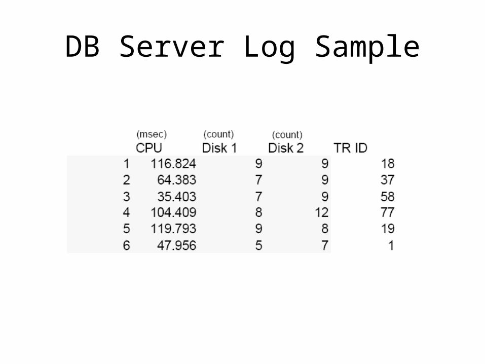
DB Server Log Sample

OS Performance Measurements

Basic Statistics for the DB ServiceWorkload
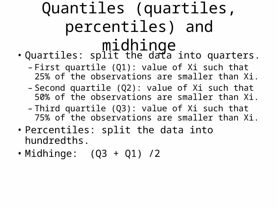
Quantiles (quartiles, percentiles) andmidhinge
• Quartiles: split the data into quarters.– First quartile (Q1): value of Xi such that 25% of the
observations are smaller than Xi.– Second quartile (Q2): value of Xi such that 50% of
the observations are smaller than Xi.– Third quartile (Q3): value of Xi such that 75% of
the observations are smaller than Xi.• Percentiles: split the data into hundredths.• Midhinge: (Q3 + Q1) /2
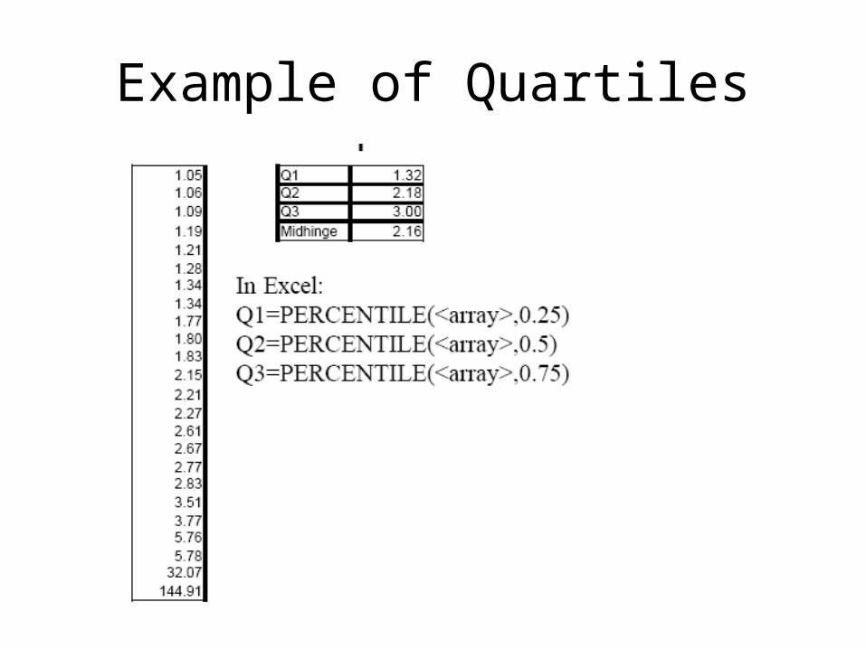
Example of Quartiles

Example of Percentile
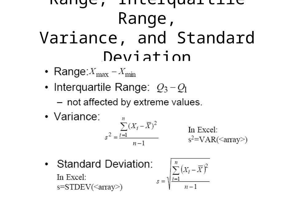
Range, Interquartile Range,Variance, and Standard Deviation
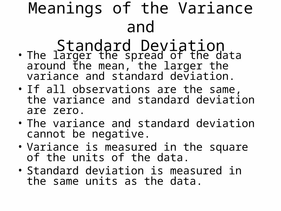
Meanings of the Variance andStandard Deviation
• The larger the spread of the data around the mean, the larger the variance and standard deviation.
• If all observations are the same, the variance and standard deviation are zero.
• The variance and standard deviation cannot be negative.
• Variance is measured in the square of the units of the data.
• Standard deviation is measured in the same units as the data.
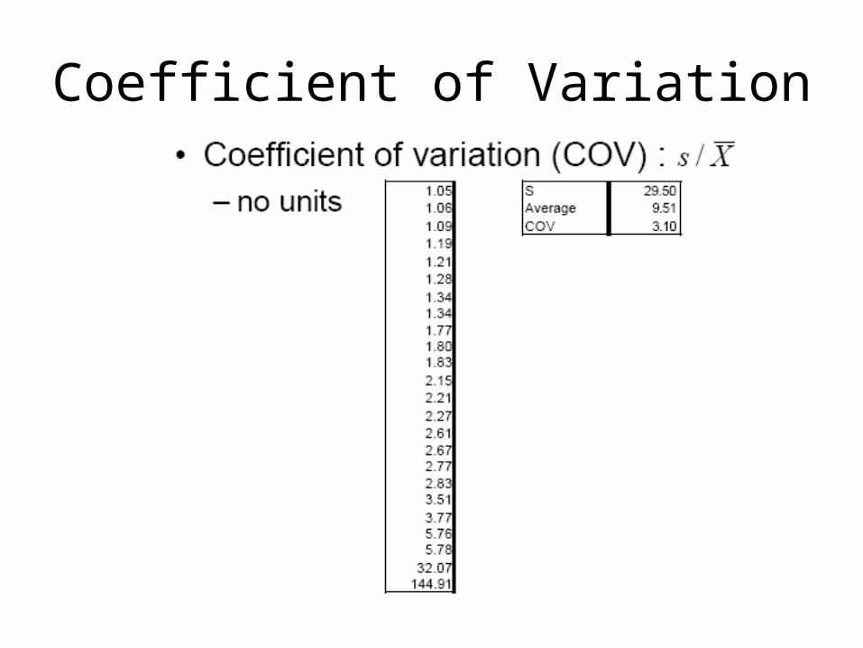
Coefficient of Variation
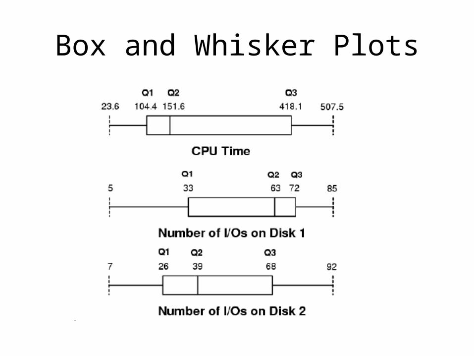
Box and Whisker Plots
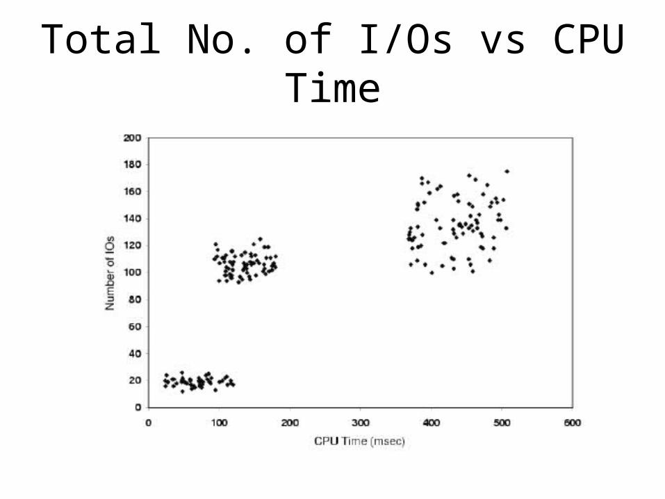
Total No. of I/Os vs CPU Time
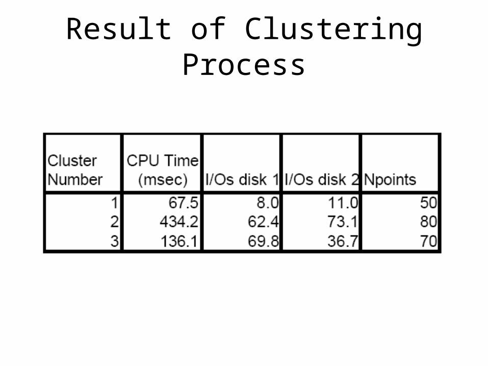
Result of Clustering Process
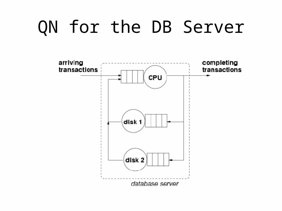
QN for the DB Server
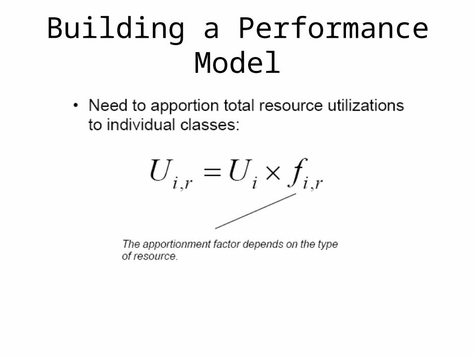
Building a Performance Model
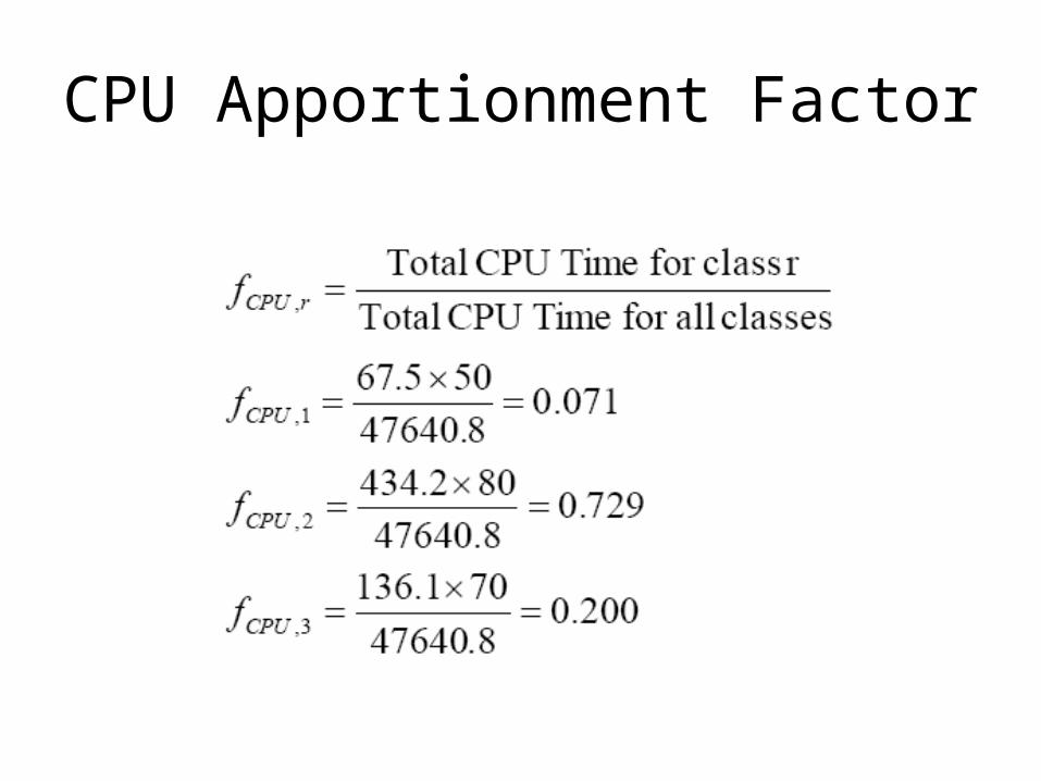
CPU Apportionment Factor
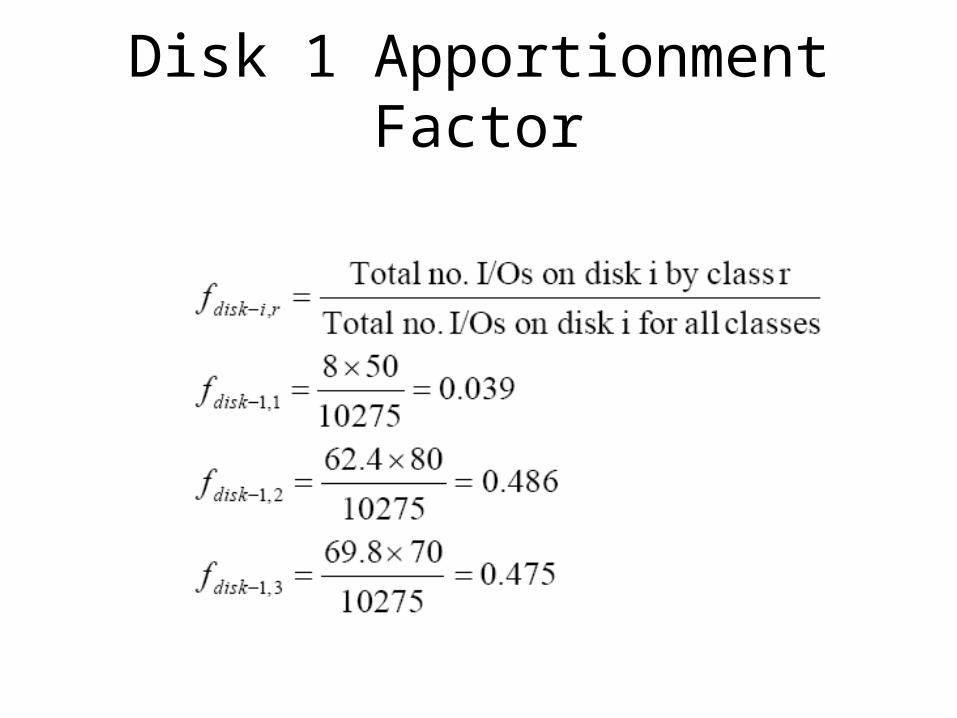
Disk 1 Apportionment Factor
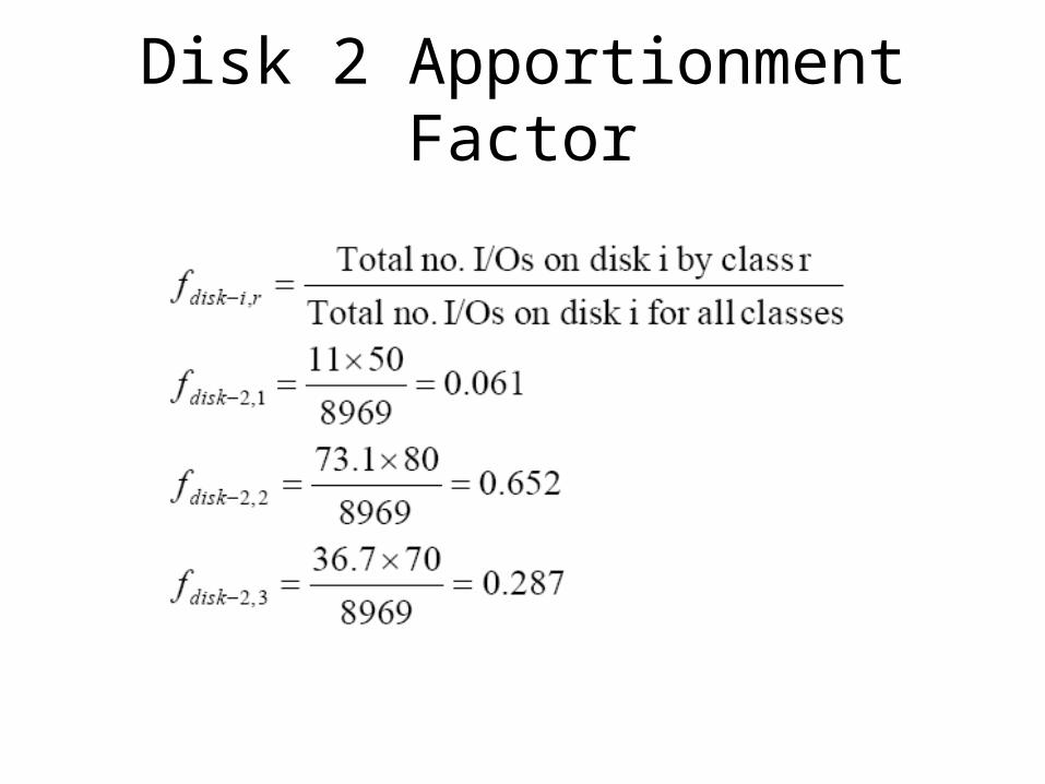
Disk 2 Apportionment Factor
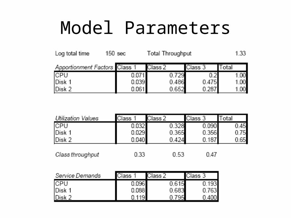
Model Parameters
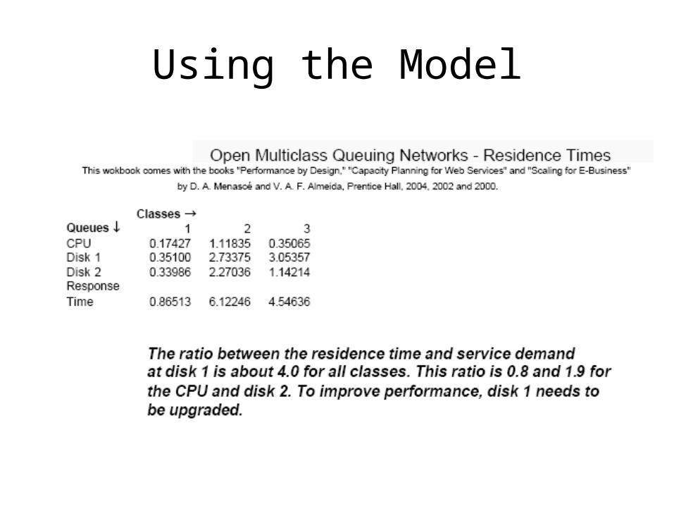
Using the Model

Workload Intensity Variation
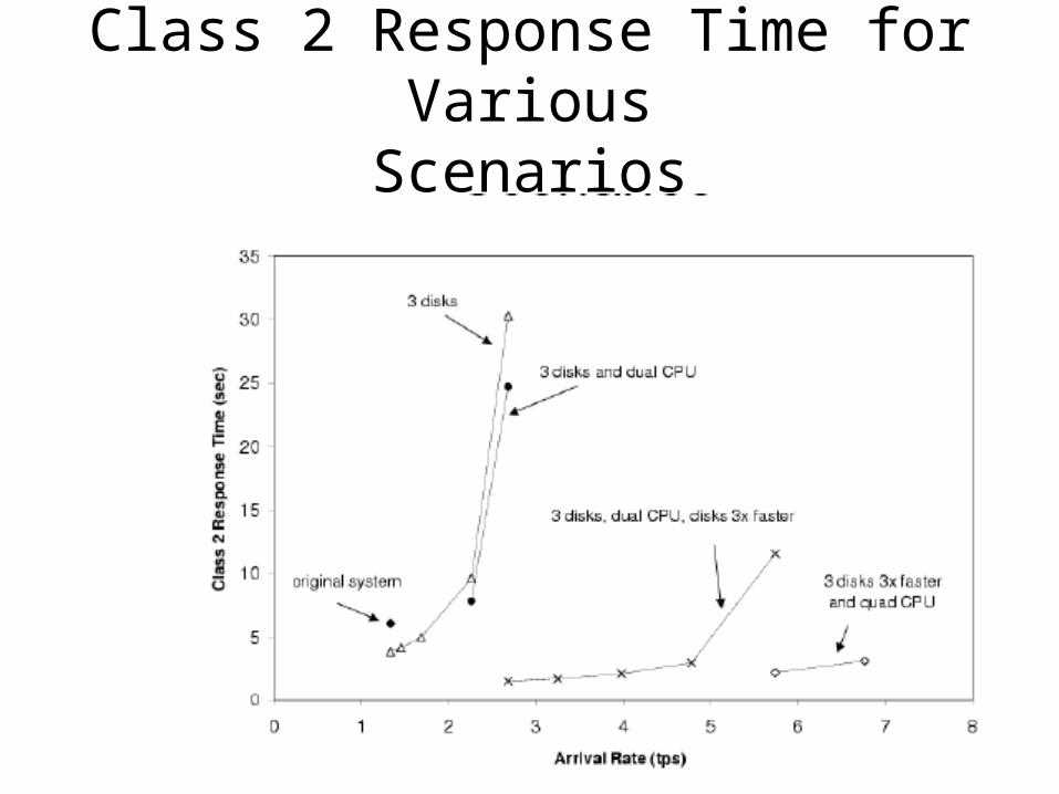
Class 2 Response Time for VariousScenarios
Monitoring Tools
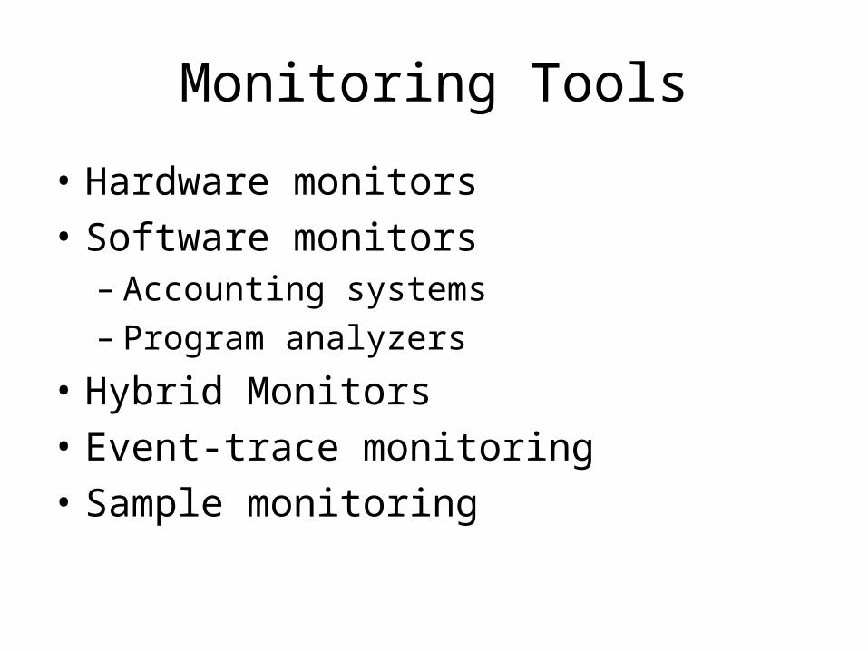
• Hardware monitors• Software monitors– Accounting systems– Program analyzers
• Hybrid Monitors• Event-trace monitoring• Sample monitoring
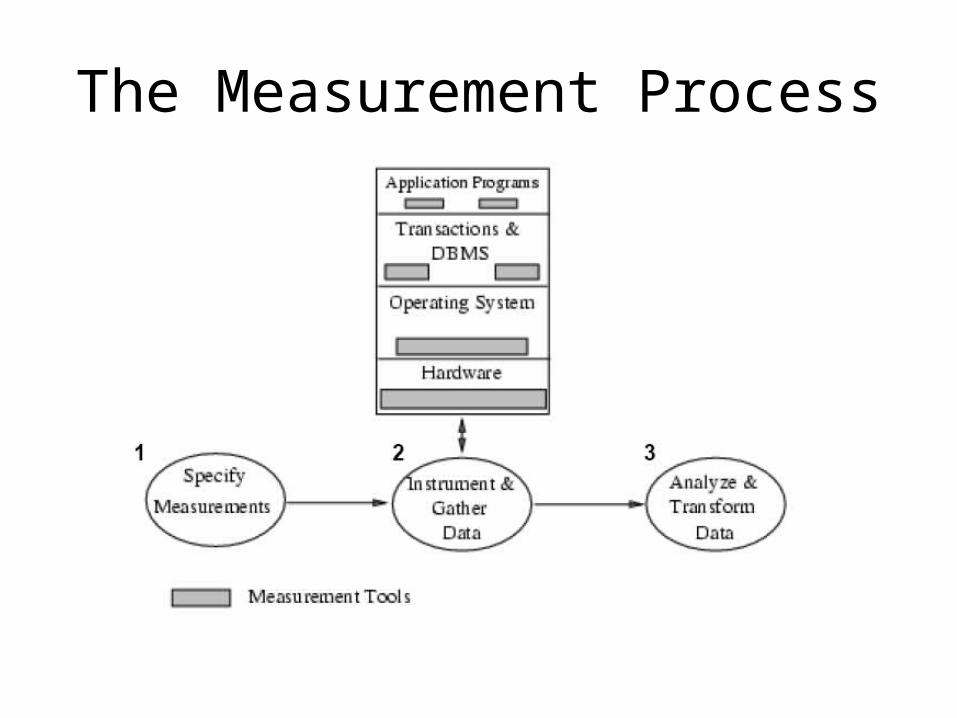
The Measurement Process

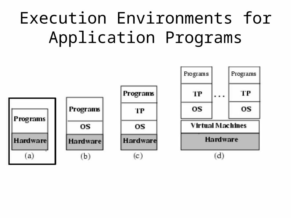
Execution Environments forApplication Programs
Execution Environments forApplication Programs
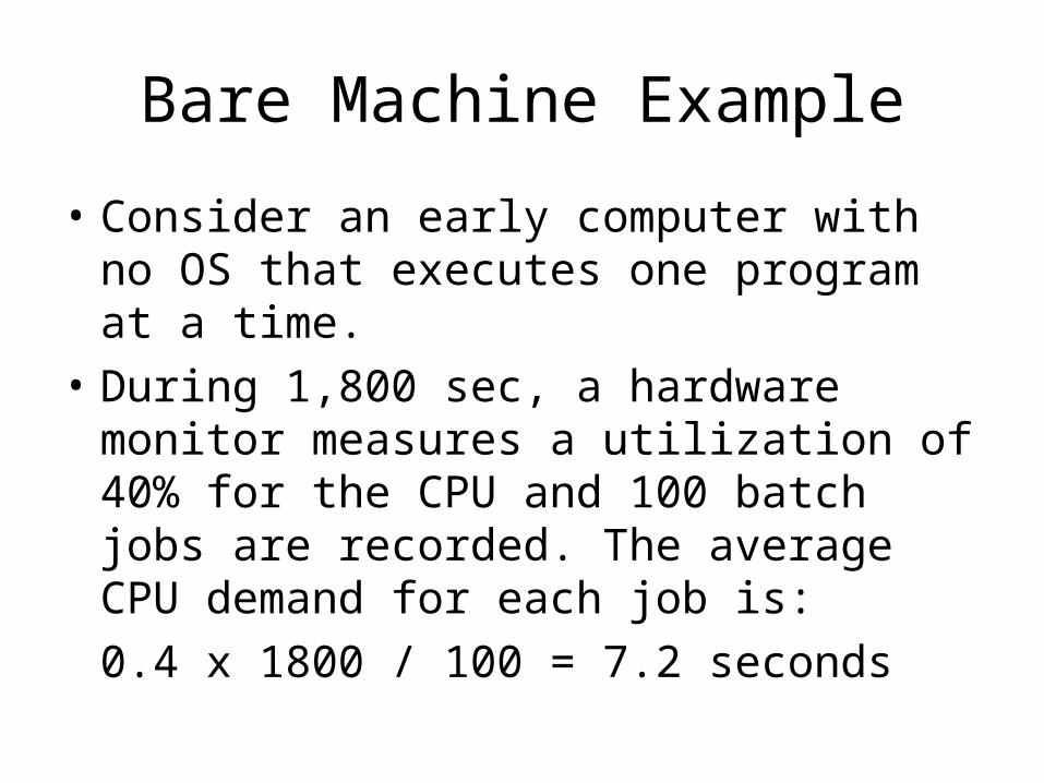
Bare Machine Example
• Consider an early computer with no OS that executes one program at a time.
• During 1,800 sec, a hardware monitor measures a utilization of 40% for the CPU and 100 batch jobs are recorded. The average CPU demand for each job is:0.4 x 1800 / 100 = 7.2 seconds
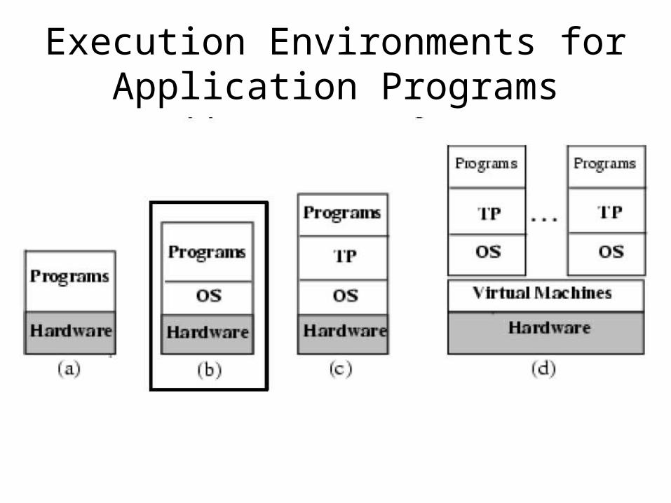
Execution Environments forApplication Programs
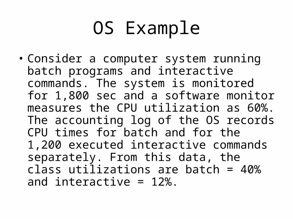
OS Example
• Consider a computer system running batch programs and interactive commands. The system is monitored for 1,800 sec and a software monitor measures the CPU utilization as 60%. The accounting log of the OS records CPU times for batch and for the 1,200 executed interactive commands separately. From this data, the class utilizations are batch = 40% and interactive = 12%.
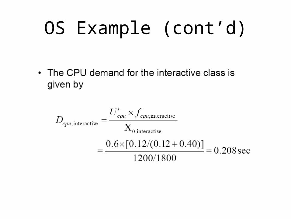
OS Example (cont’d)

Execution Environments forApplication Programs

TP Example
• A mainframe processes 3 workload• classes:– batch (B), interactive (I), and transactions (T).
• Classes B and I run on top of the OS and class T runs on top of the TP monitor.
• There are two types of transactions: – query (Q) and update (U).
• What is the service demand of update transactions?
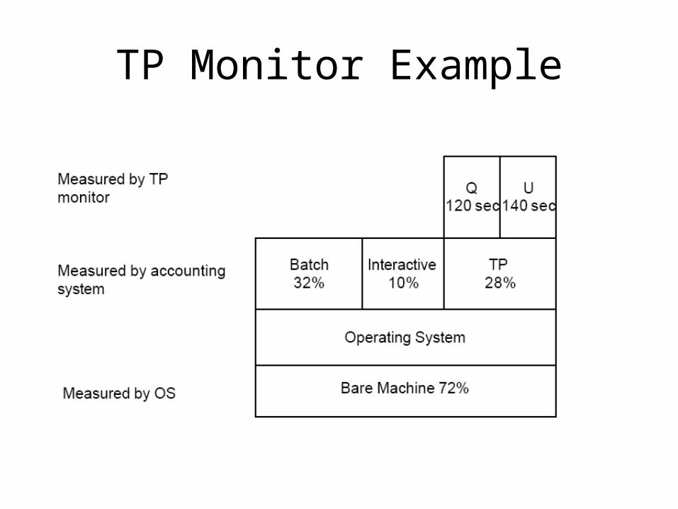
TP Monitor Example
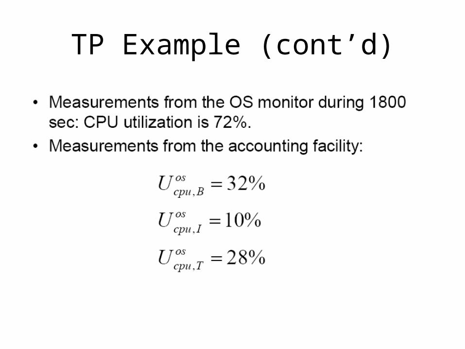
TP Example (cont’d)
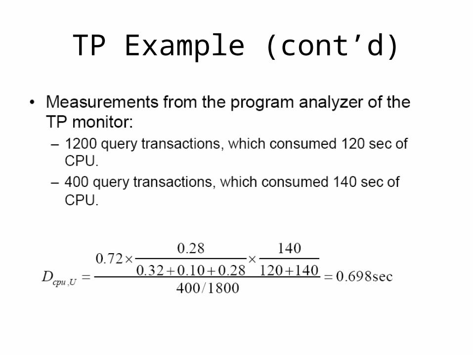
TP Example (cont’d)
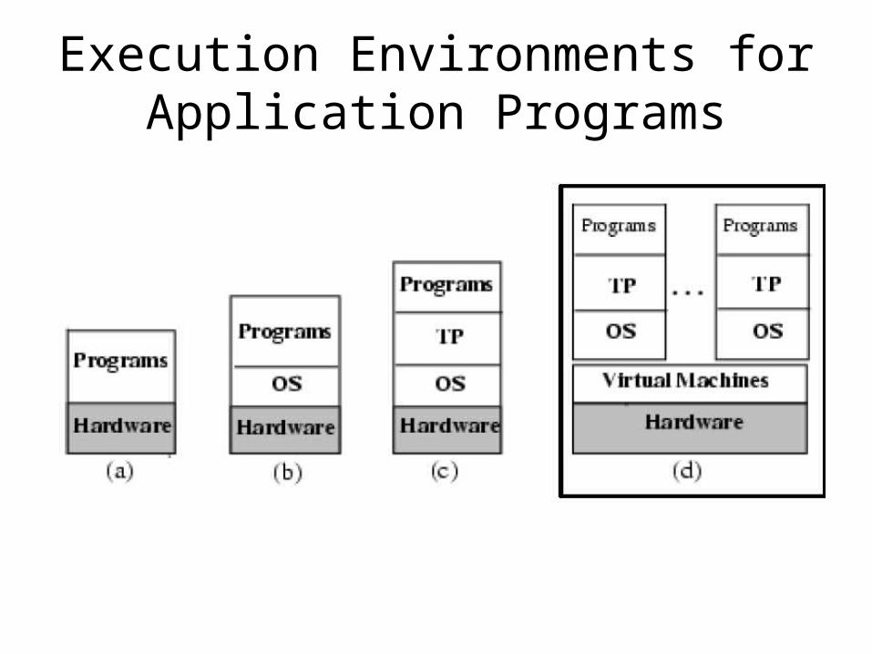
Execution Environments forApplication Programs
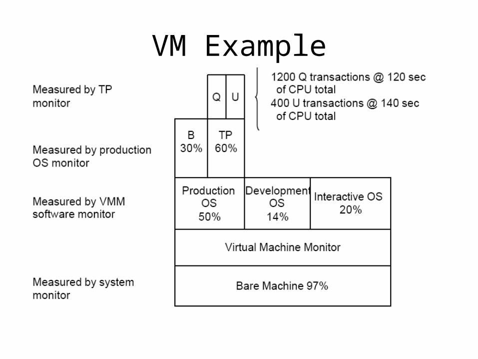
VM Example
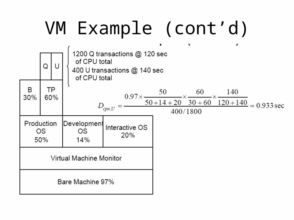
VM Example (cont’d)
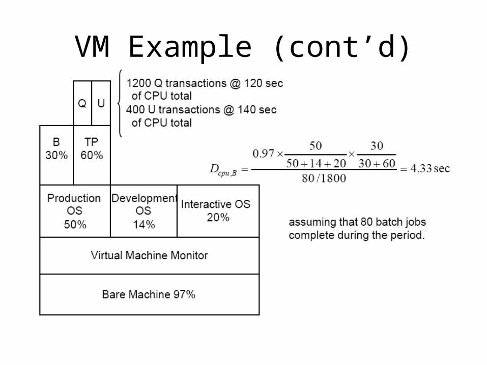
VM Example (cont’d)
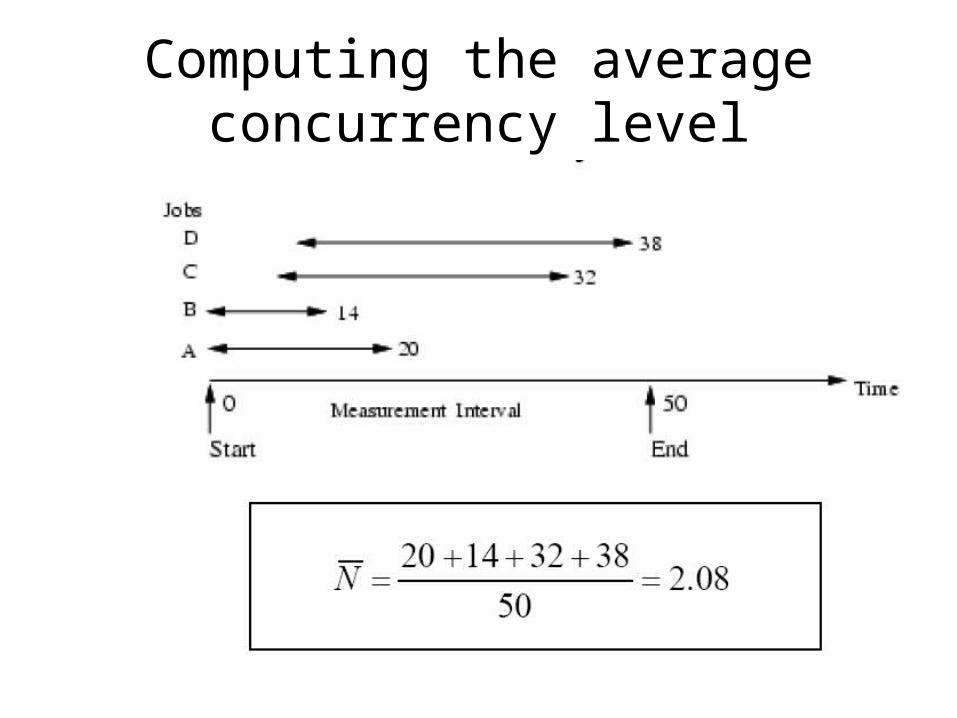
Computing the averageconcurrency level


