Page 1
University of Calgary
PRISM: University of Calgary's Digital Repository
Graduate Studies The Vault: Electronic Theses and Dissertations
2017
Case Study of Expanding Solvent-SAGD Process for
Athabasca Oil Sand Reservoirs with Presensce of
Lean Zones
Yu, Yanguo
Yu, Y. (2017). Case Study of Expanding Solvent-SAGD Process for Athabasca Oil Sand Reservoirs
with Presensce of Lean Zones (Unpublished master's thesis). University of Calgary, Calgary, AB.
doi:10.11575/PRISM/25222
http://hdl.handle.net/11023/3963
master thesis
University of Calgary graduate students retain copyright ownership and moral rights for their
thesis. You may use this material in any way that is permitted by the Copyright Act or through
licensing that has been assigned to the document. For uses that are not allowable under
copyright legislation or licensing, you are required to seek permission.
Downloaded from PRISM: https://prism.ucalgary.ca
Page 2
i
UNIVERSITY OF CALGARY
Case Study of Expanding Solvent -SAGD Process for Athabasca Oil Sand Reservoirs
with Presence of Lean Zones
by
Yanguo Yu
A THESIS
SUBMITTED TO THE FACULTY OF GRADUATE STUDIES
IN PARTIAL FULFILMENT OF THE REQUIREMENTS FOR THE
DEGREE OF MASTER OF SCIENCE
GRADUATE PROGRAM IN CHEMICAL AND PETROLEUM ENGINEERING
CALGARY, ALBERTA
JULY, 2017
© Yanguo Yu 2017
Page 3
ii
Abstract
Reservoir heterogeneities (i.e., lean zones or shale layers) impact the performance
of SAGD (steam assisted gravity drainage) processes. The lean zones, which have a water
saturation of more than 50%, have been reported by several oil sands fieldsduring the
development of oil sand reservoirs in the Athabasca area in western Canada. They reported
that the lean zones severely affected the production of SAGD processes. Therefore, an ES-
SAGD (expanding solvent SAGD) process has been introduced into this type of reservoir
to improve the production performance.
Simulation studies are conducted to investigate the mechanisms of how lean zones
influence the two processes by comparing their bottom, middle, and top locations in a
reservoir. Moreover, the thickness, location, water saturation of lean zones and reservoir
permeability are also investigated to understand the impacts of lean zones further on these
processes. A heterogeneous reservoir model, which contains lean zones, is carried out to
study the production performance of the SAGD and ES-SAGD processes.
Page 4
iii
Acknowledgements
I would like to deeply thank my supervisor Dr. Zhangxing (John) Chen for giving
me the opportunity, support, resources, guidance, and freedom to do my research work at
the University of Calgary. My profound thanks go to Dr. Pedro R. Pereira Almao and Dr.
Qingye (Gemma) Lu for their gracious willingness to serve on my exam committee. My
gratitude goes to Mr. Jinze Xu and Mr. Yuan Hu for their timely support, involvement,
knowledge, commitment, and technical help provided to me throughout my research work.
I am grateful to Mr. Christof Lee and Dr. David R. Williams for dedicating their time and
efforts in reading my thesis and giving me with their valuable feedback and suggestions. I
also would like to thank all teammates in the Reservoir Simulation Group (RSG) and all
sponsors of RSG. I also thank the assistants in RSG, Ms. Jamie McInnis, Ms. Fengyue Lin
and Mr. Stephen Cartwright for their help. To Chemical and Petroleum Department,
University of Calgary, I hope to express my appreciations to all stuff in the department.
My deepest and sincere gratitude goes to my entire family, my parents, and my
older sisters for their selfless support, motivation, and love.
This thesis is dedicated to my beloved wife, Yutao (Teresa) Niu, and my wonderful
son, Guanghong (Eric) Yu.
Page 5
iv
Table of Contents
Abstract ............................................................................................................................... ii
Acknowledgements ............................................................................................................ iii
Table of Contents ............................................................................................................... iv
List of Tables .................................................................................................................... vii
List of Figures and Illustrations ....................................................................................... viii
List of Symbols, Abbreviations, and Nomenclature ........................................................ xvi
Chapter One: : INTRODUCTION .......................................................................................1
1.1 Overview ........................................................................................................................1
1.2 Problem Statement .........................................................................................................2
1.3 Objectives of Thesis .......................................................................................................3
1.4 Organization of Thesis ...................................................................................................3
Chapter Two: REVIEW OF LITERATURE .......................................................................5
2.1 Cyclic Steam Stimulation (CSS) ....................................................................................5
2.2 Steam Flooding ..............................................................................................................6
2.3 Steam Assisted Gravity Drainage (SAGD)....................................................................8
2.3.1 Basic Analytical Model of SAGD ..........................................................................9
2.3.2 The Effects of Temperature on Bitumen Viscosity ..............................................11
2.3.3 The Process of Steam Chamber Development .....................................................13
2.3.4 Review of Operation Parameters in SAGD Process .............................................14
2.3.4.1 Start-up in SAGD Process ............................................................................14
2.3.4.2 Steam Trap Control in SAGD Process .........................................................16
2.3.4.3 Operation Pressure in SAGD (Low pressure vs. High pressure) .................17
2.3.5 Improvement of SAGD Process ...........................................................................19
2.4 Expanding Solvent - Steam Assisted Gravity Drainage (ES-SAGD) ..........................19
2.4.1 Basic Theory of Expanding Solvent - SAGD (ES-SAGD) ..................................20
2.4.2 Solvent Selection of ES-SAGD Process ...............................................................21
2.4.3 Effects of Solvent Concentration on ES-SAGD Process ......................................26
2.4.4 The Impacts of Operating Pressure .......................................................................27
2.4.5 Phase Behavior of Steam Chamber in ES-SAGD Process ...................................28
2.5 The Impacts of Reservoir Heterogeneities ...................................................................32
Chapter Three: RESERVOIR MODEL .............................................................................36
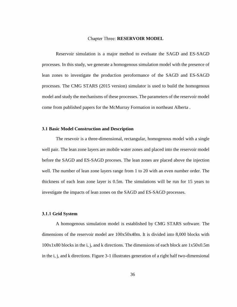
3.1 Basic Model Construction and Description .................................................................36
3.1.1 Grid System ..........................................................................................................36
3.1.2 Reservoir Properties ..............................................................................................39
3.2 Fluid Properties ............................................................................................................41
3.3 Operation Parameters for the Cases .............................................................................42
3.4 The Location of Lean Zones in the Reservoir Model ..................................................42
Chapter Four: DISCUSSION OF SAGD PROCESS WITH LEAN ZONES ...................43
4.1 Introduction ..................................................................................................................43
4.2 The Comparison of Base Case and Lean Zones (2 meters) Case ................................43
Page 6
v
4.2.1 Analysis and Comparison of the Steam Chamber ................................................44
4.2.1.1 Bottom Area of the Reservoir .......................................................................47
4.2.1.2 Middle Area of the Reservoir .......................................................................51
4.2.1.3 Top Area of the Reservoir ............................................................................54
4.2.2 Comparative Analysis of the Impacts of Lean Zones in the Reservoir ................57
4.2.2.1 Water Saturation and Velocity Vector of Water Distribution ......................57
4.2.2.2 Production Variations in the Steam Chamber ..............................................59
4.2.3 Comparison and Analysis of the Growth of the Steam Chamber .........................61
4.3 Sensitivity Analysis of Reservoir with Lean Zones in SAGD Process .......................64
4.4 Conclusions of the SAGD Process ..............................................................................66
Chapter Five: ANALYSIS OF ES-SAGD PROCESS WITH LEAN ZONES..................68
5.1 Introduction ..................................................................................................................68
5.2 Solvent Characterization ..............................................................................................68
5.3 Solvent Injection Strategies .........................................................................................69
5.4 Results Discussion and Comparison of Base Cases and Lean Zones Cases ...............69
5.4.1 Mechanisms Analysis of Reservoir at Different Locations ..................................72
5.4.1.1 Bottom of the Reservoir ...............................................................................72
5.4.1.2 Middle of the Reservoir ................................................................................78
5.4.1.3 Top of the Reservoir .....................................................................................83
5.4.2 Impacts of Lean Zones in the Reservoir ...............................................................89
5.4.2.1 Temperature Distribution .............................................................................89
5.4.2.2 Distribution of the Water Saturation and Velocity Vector of Water ............91
5.4.3 Solvent Distribution in the Steam Chamber .........................................................94
5.4.3.1 Mole Fraction Distribution of IC4-NC5 ........................................................94
5.4.3.2 Mole Fraction Distribution of C6-C8 ............................................................96
5.4.4 Comparison of Production Performance ...............................................................97
5.4.5 Comparative Analysis of the Growth of the Steam Chamber ..............................99
5.4.6 Solvent Distribution in the Growth of the Steam Chamber ................................102
5.5 Sensitivity Analysis of Reservoir with Lean Zones in ES-SAGD Process ...............107
5.5.1 Multiple-layer of the Lean Zones .......................................................................107
5.5.2 The Locations of the Lean Zones .......................................................................108
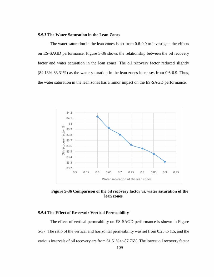
5.5.3 The Water Saturation of the Lean Zones ............................................................109
5.5.4 The Effect of Reservoir Vertical Permeability ...................................................109
5.6 Conclusions of the ES-SAGD Process ......................................................................111
Chapter Six: COMPARISON OF SAGD AND ES-SAGD PROCESSES IN RESERVOIR
WITH LEAN ZONES......................................................................................................113
6.1 Introduction ................................................................................................................113
6.2 Comparative Mechanism Analyses of Reservoir at Different Locations ..................113
6.2.1 Comparison at Lean Zone Area ..........................................................................116
6.2.2 Comparison of the Middle of the Reservoir .......................................................118
6.2.3 Comparison of the Bottom of the Reservoir .......................................................121
6.3 Comparison of Growth of the Steam Chamber in SAGD and ES-SAGD Processes 125
6.4 Comparative Analysis and Discussion for Lean Zones .............................................128
Page 7
vi
Temperature Distribution ....................................................................................128
Water Distribution and Velocity Vector of Water ..............................................129 Oil Mobility Distribution ....................................................................................130 Thickness of the Lean Zones ..............................................................................131
Comparison of SAGD and ES-SAGD Processes in a Heterogeneous Reservoir ......134 2D Heterogeneous Model Construction and Description ...................................134 Operation Parameters ..........................................................................................135 Results and Discussion .......................................................................................138
Conclusions of the Chapter ........................................................................................140
CONCLUSIONS AND FUTURE WORKS ..........................................141 Conclusions ................................................................................................................141 Future Works .............................................................................................................142
REFERENCES ................................................................................................................143
Page 8
vii
List of Tables
Table 3-1 Reservoir Parameters for Simulation Model .................................................... 39
Page 9
viii
List of Figures and Illustrations
Figure 1-1 Oil sand deposits in Alberta (Government of Alberta 2012) ............................ 1
Figure 2-1 Cyclic steam stimulation process (Oilberta Oil & Gas Corp.) .......................... 5
Figure 2-2 Steam flooding process (Petroleum Support Corp.) ......................................... 7
Figure 2-3 Steam assisted gravity drainage (SAGD) process (JPEC) ................................ 8
Figure 2-4 Viscosity of Athabasca bitumen vs. temperature ............................................ 12
Figure 2-5 Basic concept of steam chamber (Butler 1981) .............................................. 13
Figure 2-6 Schematic of start-up procedure in SAGD process (Rangewest Tech.) ......... 15
Figure 2-7 Schematic of an ideal steam chamber in SAGD Process (Gates 2010). ......... 16
Figure 2-8 Basic concept of Expanding Solvent – SAGD (ES-SAGD) ........................... 21
Figure 2-9 Comparison of hydrocarbons (C3 to C8) vaporization temperature with steam
temperature (Nasr et al. 2003)................................................................................... 23
Figure 2-10 Comparison of oil drainage rates and different hydrocarbon co-injecting
strategies (Nasr et al. 2003)....................................................................................... 24
Figure 2-11 Oil drainage rates vs. temperature difference between steam and solvent
(Nasr et al. 2003) ....................................................................................................... 25
Figure 2-12 Solvent (C6) volume fraction vs. viscosity of Athabasca bitumen at
constant temperature (Li 2010) ................................................................................. 27
Figure 2-13 Correlation between condensation temperature of water and hexane
mixture versus mole fraction of hexane at 2000 kPa (Dong 2012) .......................... 30
Figure 2-14 Correlation between condensation temperature of water and hexane
mixture versus volume fraction of hexane at 2000 kPa (calculated at 25 oC) (Dong
2012) ......................................................................................................................... 31
Figure 2-15 Temperature profiles in distance at the edge of steam chamber between
SAGD and ES-SAGD (More Fraction of Hexane at 0.01, 2000 kPa) (Dong 2012)
................................................................................................................................... 31
Figure 3-1 Grid structure of a right half reservoir model in i-k directions ....................... 37
Figure 3-2 A right half reservoir model in 3D view ......................................................... 38
Page 10
ix
Figure 3-3 Water–oil relative permeabilility, ................................................................... 40
Figure 3-4 Gas-liquid relative permeability, ..................................................................... 40
Figure 3-5 The correlation of temperature versus bitumen viscosity ............................... 41
Figure 4-1Water saturation profile in cross-section of SAGD ......................................... 43
Figure 4-2 Comparison of the temperature distributions with different zones of SAGD
process with 2500 kPa injection pressure at 273 days .............................................. 45
Figure 4-3 Schematic presentation of the temperature, gas saturation, oil saturation, oil
mobility, water saturation profiles along the line of study (50-67 m) in SAGD
process with 2500 kPa injection pressure at 273 days .............................................. 46
Figure 4-4 Comparison of the temperature profiles with three areas of the reservoir in
SAGD with 2500 kPa injection pressure at 273 days ............................................... 46
Figure 4-5 Comparison of the temperature profiles at bottom area of the reservoir with
2500 kPa injection pressure at 273 days. The dashed line indicates the location of
study line ................................................................................................................... 49
Figure 4-6 Schematic representation of the temperature, gas saturation, oil saturation,
oil mobility, water saturation profiles along the line of study (50-65 m) in SAGD
process with 2500 kPa injection pressure at 273 days .............................................. 50
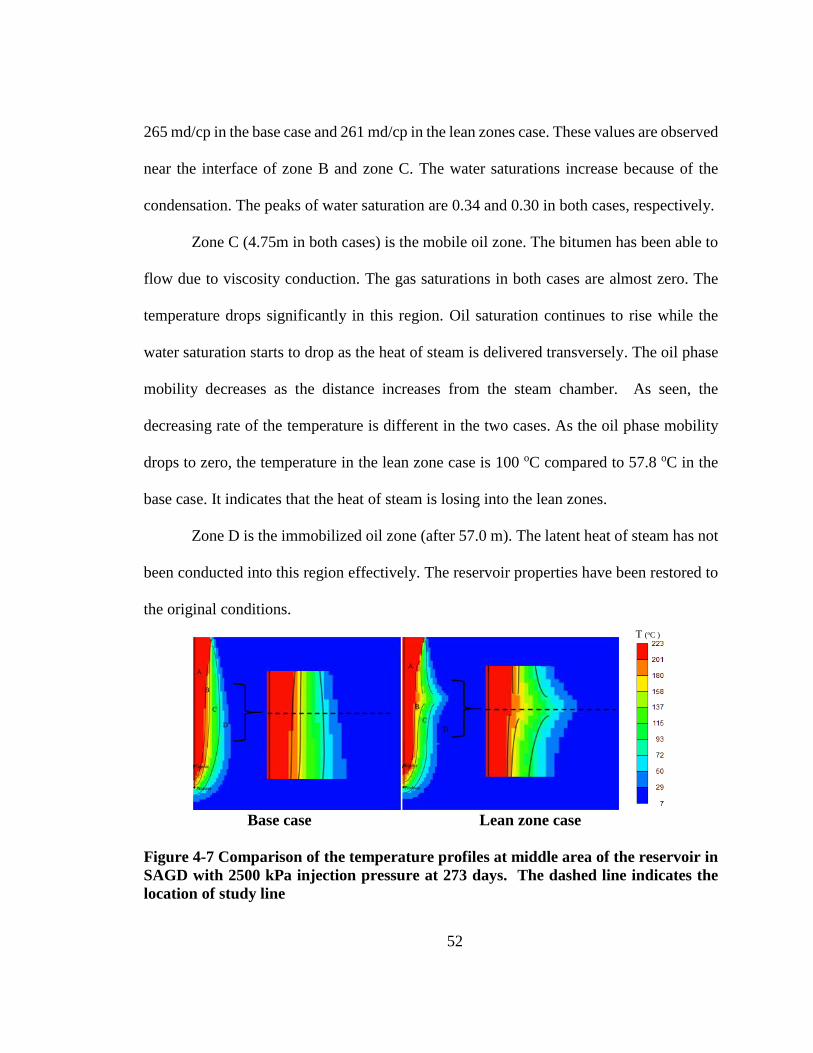
Figure 4-7 Comparison of the temperature profiles at middle area of the reservoir in
SAGD with 2500 kPa injection pressure at 273 days. The dashed line indicates
the location of study line ........................................................................................... 52
Figure 4-8 Schematic representation of the temperature, gas saturation, oil saturation,
oil mobility, water saturation profiles along the line of study (50-65m) in SAGD
process with 2500 kPa injection pressure at 273 days .............................................. 53
Figure 4-9 Comparison of the temperature profiles at top area of the reservoir in SAGD
process with 2500 kPa injection pressure at 273 days. The dashed line indicates
the location of the line of study. ................................................................................ 55
Figure 4-10 Schematic representation of the temperature, gas saturation, oil saturation,
oil mobility, water saturation profiles along the line of study (50-65 m) in SAGD
with 2500 kPa injection pressure at 273 days ........................................................... 56
Figure 4-11 Comparison of water saturation and water velocity vector in SAGD with
2500 kPa injection pressure at 273 days. .................................................................. 58
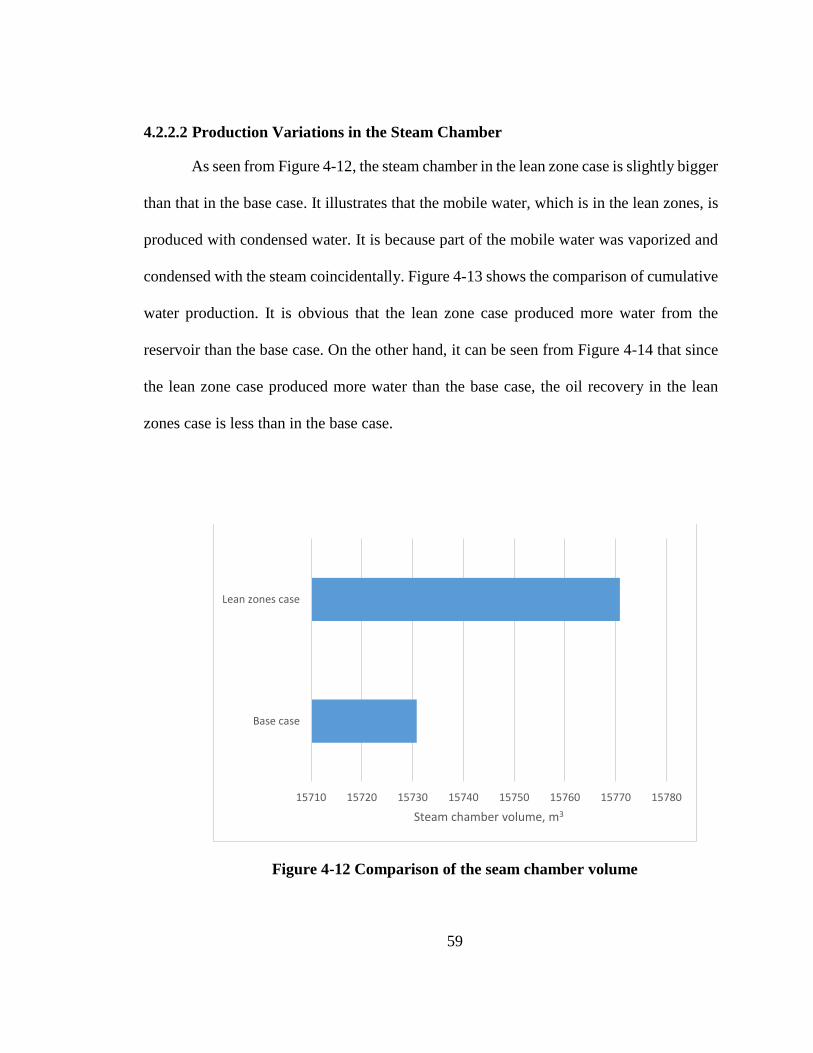
Figure 4-12 Comparison of the seam chamber volume .................................................... 59
Page 11
x
Figure 4-13 Comparison of the cumulative water production .......................................... 60
Figure 4-14 Comparison of the oil recovery factor .......................................................... 60
Figure 4-15 Comparison of the temperature profiles in cross section of SAGD with
2500 kPa injection pressure at 180 days, 365 days, and 730 days ........................... 62
Figure 4-16 Comparison of the gas saturation profiles in cross section of SAGD with
2500 kPa injection pressure at 180 days, 365 days, and 730 days. ........................... 63
Figure 4-17 Comparison of the oil recovery factor vs. thickness of the lean zones ......... 65
Figure 4-18 Effects of the lean zone water saturation vs. the oil recovery factor ............ 65
Figure 4-19 Effects of the ratio of vertical and horizontal permeabilty vs. the oil
recovery factor .......................................................................................................... 66
Figure 5-1 Comparison of the temperature profiles with different zones of ES-SAGD
process with 2500 kPa injection pressure at 273 days. The dished line is the study
line ............................................................................................................................. 70
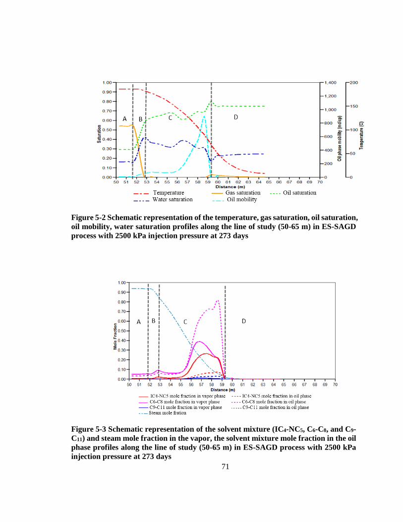
Figure 5-2 Schematic representation of the temperature, gas saturation, oil saturation,
oil mobility, water saturation profiles along the line of study (50-65 m) in ES-
SAGD process with 2500 kPa injection pressure at 273 days .................................. 71
Figure 5-3 Schematic representation of the solvent mixture (IC4-NC5, C6-C8, and C9-
C11) and steam mole fraction in the vapor, the solvent mixture mole fraction in the
oil phase profiles along the line of study (50-65 m) in ES-SAGD process with
2500 kPa injection pressure at 273 days ................................................................... 71
Figure 5-4 Comparison of the temperature profiles with three areas of the reservoir in
ES-SAGD with 2500 kPa injection pressure at 273 days ......................................... 72
Figure 5-5 Comparison of temperature profiles at bottom location of the reservoir in
ES-SAGD process with 2500 kPa injection pressure at 273 days. The dashed line
indicates the location of study line ............................................................................ 75
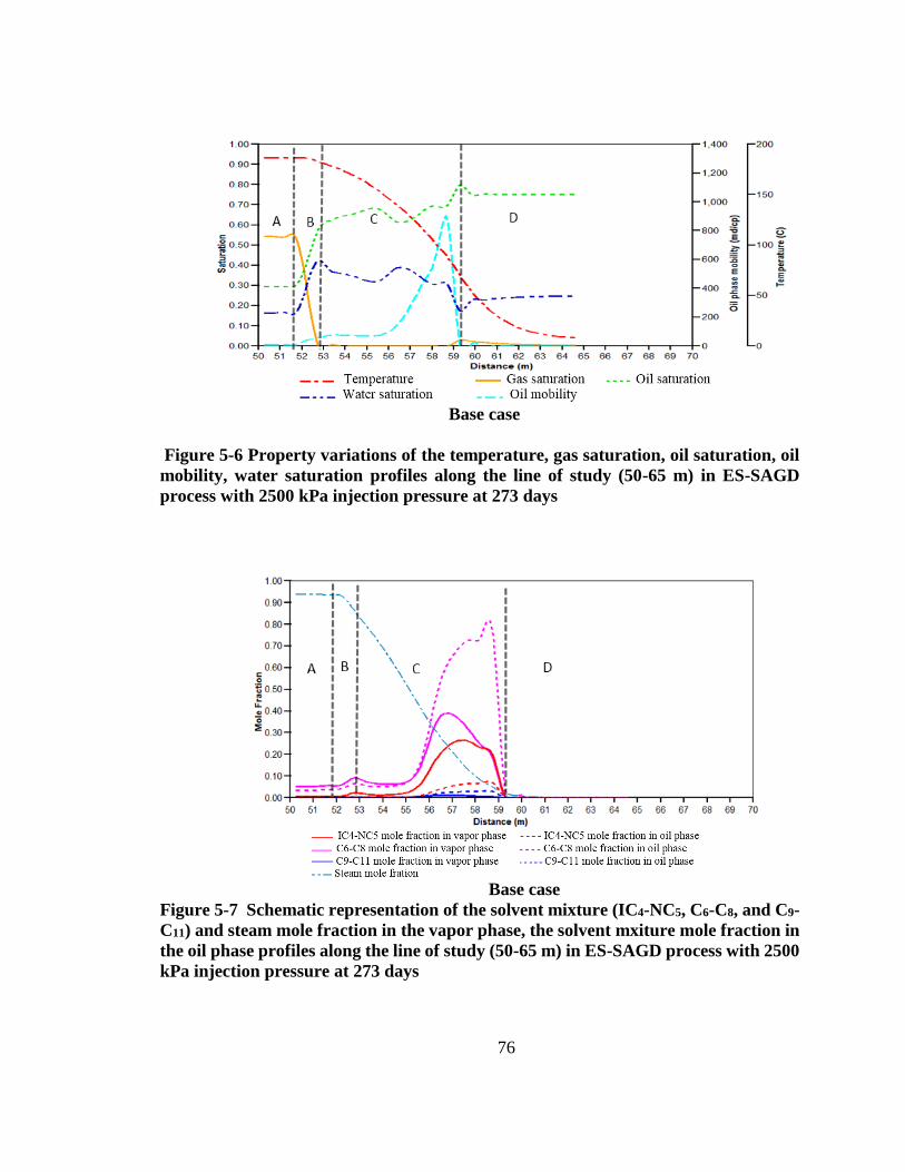
Figure 5-6 Property variations of the temperature, gas saturation, oil saturation, oil
mobility, water saturation profiles along the line of study (50-65 m) in ES-SAGD
process with 2500 kPa injection pressure at 273 days .............................................. 76
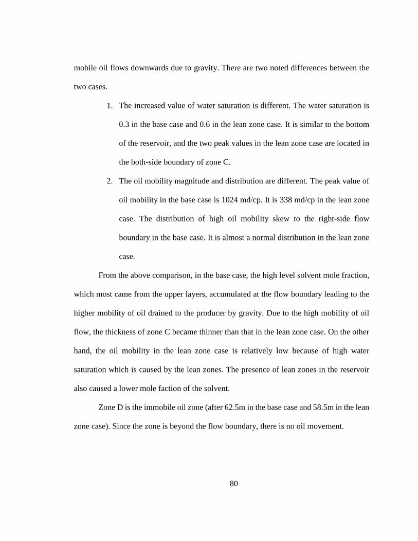
Figure 5-7 Schematic representation of the solvent mixture (IC4-NC5, C6-C8, and C9-
C11) and steam mole fraction in the vapor phase, the solvent mxiture mole fraction
in the oil phase profiles along the line of study (50-65 m) in ES-SAGD process
with 2500 kPa injection pressure at 273 days ........................................................... 76
Page 12
xi
Figure 5-8 Property variations of the temperature, gas saturation, oil saturation, oil
mobility, water saturation profiles along the line of study (50-65 m) in ES-SAGD
process with 2500 kPa injection pressure at 273 days .............................................. 77
Figure 5-9 Schematic representation of the solvent mixture (IC4-NC5, C6-C8, and C9-
C11) and steam mole fraction in the vapor phase, solvent mxiture mole fraction in
the oil phase profiles along the line of study (50-65 m) in ES-SAGD process with
2500 kPa injection pressure at 273 days ................................................................... 77
Figure 5-10 Comparison of the temperature profiles at middle location of the reservoir
in ES-SAGD process with 2500 kPa injection pressure at 273 days. The dashed
line indicates the location of study line ..................................................................... 81
Figure 5-11 Property variations of the temperature, gas saturation, oil saturation, oil
mobility, water saturation profiles along the line of study (50-65 m) in ES-SAGD
process with 2500 kPa injection pressure at 273 days .............................................. 81
Figure 5-12 Schematic representation of the solvent (IC4-NC5, C6-C8, and C9-C11) and
steam mole fraction in vapor phase, the solvent mixture mole fraction in the oil
phase profiles along the line of study (50-65 m) in ES-SAGD process with 2500
kPa injection pressure at 273 days ............................................................................ 82
Figure 5-13 Property variations of the temperature, gas saturation, oil saturation, oil
mobility, water saturation profiles along the line of study (50-65 m) in ES-SAGD
process with 2500 kPa injection pressure at 273 days. ............................................. 82
Figure 5-14 Schematic representation of the solvent (IC4-NC5, C6-C8, and C9-C11) and
steam mole fraction in the vapor phase, the solvent mixture mole fraction in the
oil phase profiles along the line of study (50-65 m) in ES-SAGD process with
2500 kPa injection pressure at 273 days ................................................................... 83
Figure 5-15 Comparison of the temperature profiles at top location of the reservoir in
ES-SAGD process with 2500 kPa injection pressure at 273 days. The dashed line
indicates the location of study line ............................................................................ 86
Figure 5-16 Property variations of the temperature, gas saturation, oil saturation, oil
mobility, water saturation profiles along the line of study (50-65 m) in ES-SAGD
process with 2500 kPa injection pressure at 273 days .............................................. 87
Figure 5-17 Schematic representation of the solvent (IC4-NC5, C6-C8, and C9-C11) and
steam mole fraction in vapor phase, the solvent mixture mole fraction in the oil
phase profiles along the line of study (50-65 m) in ES-SAGD process with 2500
kPa injection pressure at 273 days ............................................................................ 87
Page 13
xii
Figure 5-18 Property variations of the temperature, gas saturation, oil saturation, oil
mobility, water saturation profiles along the line of study (50-65 m) in ES-SAGD
process with 2500 kPa injection pressure at 273 days .............................................. 88
Figure 5-19 Schematic representation of the solvent (IC4-NC5, C6-C8, and C9-C11) and
steam mole fraction in vapor phase, the solvent mixture mole fraction in the oil
phase profiles along the line of study (50-65 m) in ES-SAGD process with 2500
kPa injection pressure at 273 days ............................................................................ 88
Figure 5-20 Comparison of temperature profiles vs. distances in SAGD with 2500 kPa
injection pressure at 273 days ................................................................................... 90
Figure 5-21 Comparison of water saturation and water velocity vector of in ES-SAGD
with 2500 kPa injection pressure at 273 days ........................................................... 93
Figure 5-22 Comparison of the solvent (IC4-NC5) mole fraction profiles in the vapor
phase of ES-SAGD with 2500 kPa injection pressure at 273 days ........................... 95
Figure 5-23 Comparison of the solvent (IC4-NC5) mole fraction profiles in the oil phase
of ES-SAGD with 2500 kPa injection pressure at 273 days ..................................... 95
Figure 5-24 Comparison of the solvent (C6-C8) mole fraction distribution in the vapor
phase of ES-SAGD with 2500 kPa injection pressure at 273 days ........................... 96
Figure 5-25 Comparison of the solvent (C6-C8) mole fraction distribution in the oil
phase of ES-SAGD with 2500 kPa injection pressure at 273 days ........................... 97
Figure 5-26 Comparison of the steam chamber volume ................................................... 98
Figure 5-27 Comparison of the oil recovery factor .......................................................... 98
Figure 5-28 Comparison of temperature profiles in cross section of ES-SAGD with
2500 kPa injection pressure at 180, 365, and 730 days .......................................... 100
Figure 5-29 Comparison of gas saturation profiles in cross section of ES-SAGD with
2500 kPa injection pressure at 180, 365, and 730 days .......................................... 101
Figure 5-30 Comparison of the solvent (IC4-NC5) mole fraction profiles in the vapor
phase of ES-SAGD with 2500 kPa injection pressure at 180, 365, and 730 days .. 103
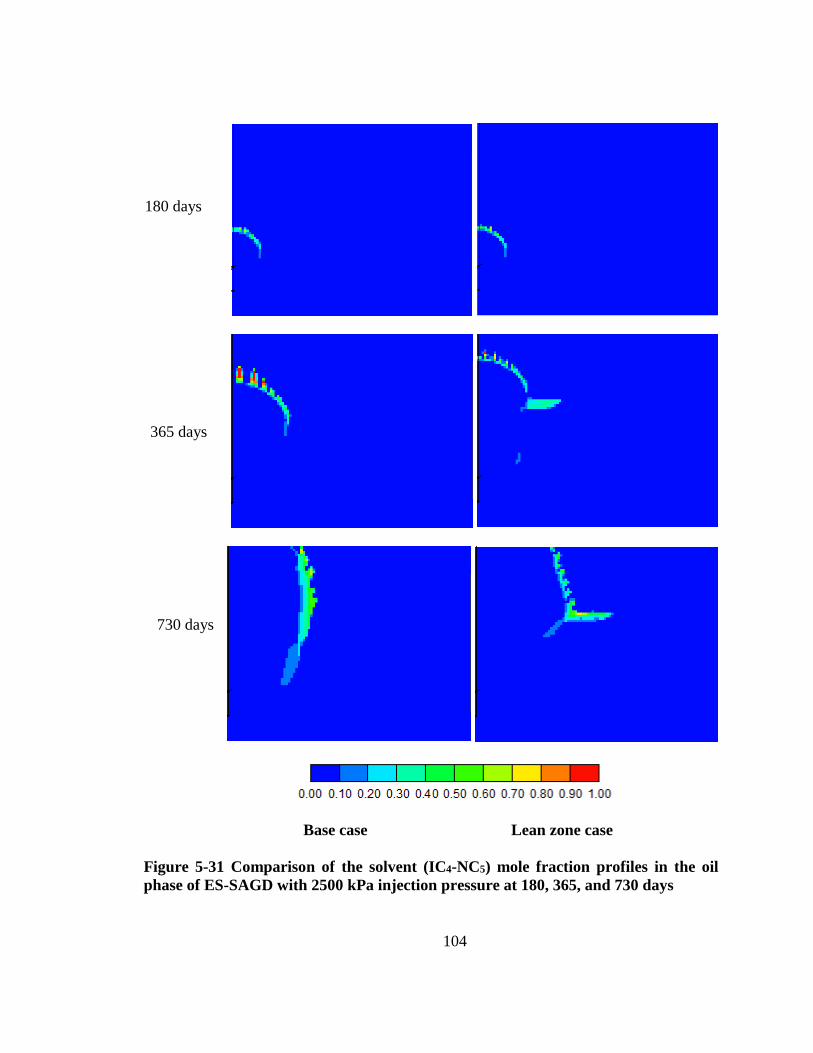
Figure 5-31 Comparison of the solvent (IC4-NC5) mole fraction profiles in the oil phase
of ES-SAGD with 2500 kPa injection pressure at 180, 365, and 730 days ............ 104
Figure 5-32 Comparison of the solvent (C6-C8) mole fraction profiles in the vapor phase
of ES-SAGD with 2500 kPa injection pressure at 180, 365, and 730 days ............ 105
Page 14
xiii
Figure 5-33 Comparison of the solvent (C6-C8) mole fraction profiles in the oil phase
of ES-SAGD with 2500 kPa injection pressure at 180, 365, and 730 days ............ 106
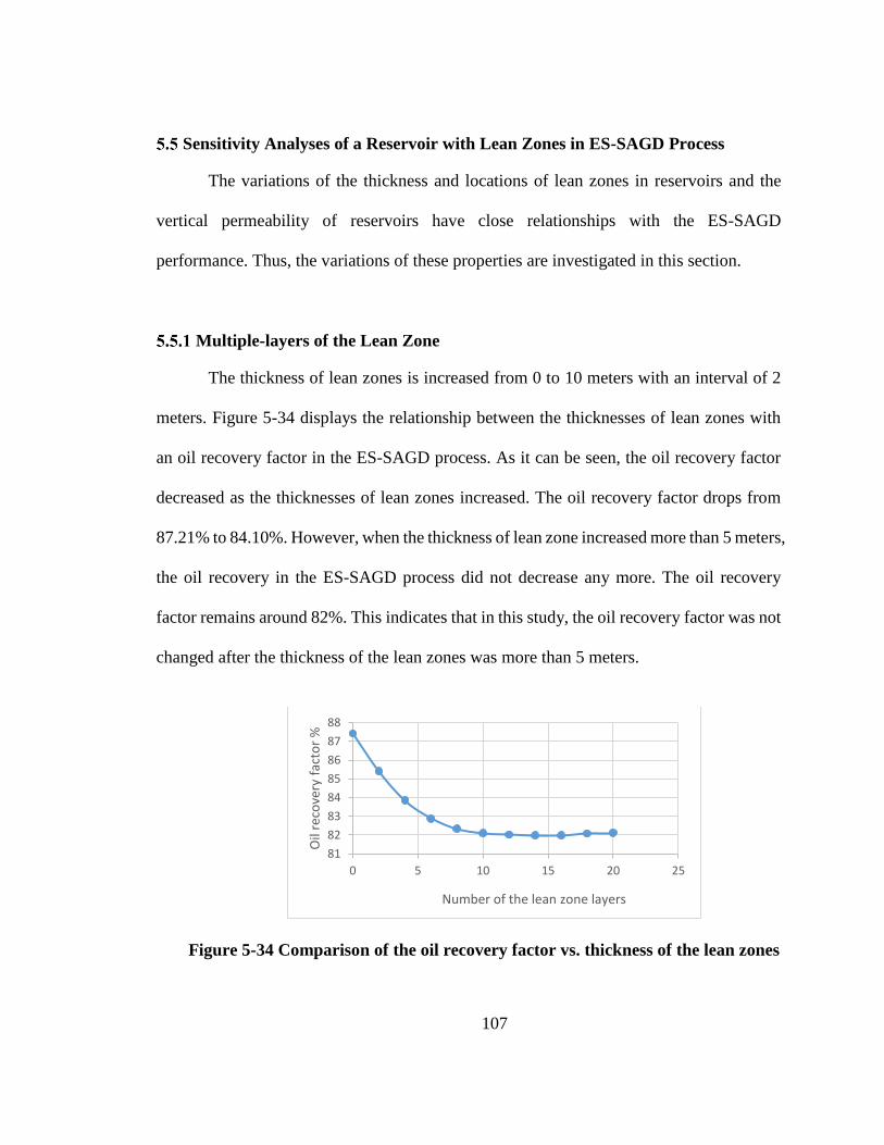
Figure 5-34 Comparison of the oil recovery factor vs. thickness of the lean zones ....... 107
Figure 5-35 Comparison of the oil recovery factor vs. location of the lean zones ......... 108
Figure 5-36 Comparison of the oil recovery factor vs. water saturation of the lean zones
................................................................................................................................. 109
Figure 5-37 Comparison of the oil recovery factor vs. the ratio of vertical and horizontal
permeability ............................................................................................................ 110
Figure 6-1 Comparison of the temperature profiles in SAGD and ES-SAGD processes
with 2500 kPa injection pressure at 273 days ......................................................... 115
Figure 6-2 Comparison of the temperature profiles in SAGD and ES-SAGD processes
with 2500 kPa injection pressure at 273 Days. The dashed line indicates the
locations of study lines ............................................................................................ 115
Figure 6-3 Property variations of the temperature, gas saturation, oil saturation, oil
mobility, water saturation profiles along the line of study (50-65 m) at lean zones
location in SAGD process with 2500 kPa injection pressure at 273 days .............. 117
Figure 6-4 Property variations of the temperature, gas saturation, oil saturation, oil
mobility, water saturation profiles along the line of study (50-65 m) at lean zone
location in ES-SAGD process with 2500 kPa injection pressure at 273 days ........ 117
Figure 6-5 Schematic representation of the solvent mixture (IC4-NC5, C6-C8, and C9-
C11) and steam mole fraction in the vapor phase, the solvent mixture mole fraction
in the oil profiles along the line of study (50-65 m) in ES-SAGD process with
2500 KPa injection pressure at 273 days ................................................................ 118
Figure 6-6 Property variations of the temperature, gas saturation, oil saturation, oil
mobility, water saturation profiles along the line of study (50-65 m) at middle
lcocation in SAGD process with 2500 kPa injection pressure at 273 days ............ 120
Figure 6-7 Property variations of the temperature, gas saturation, oil saturation, oil
mobility, water saturation profiles along the line of study (50-65 m) at middle
location in ES-SAGD process with 2500 kPa injection pressure at 273 days ........ 120
Figure 6-8 Schematic representation of the solvent mixture (IC4-NC5, C6-C8, and C9-
C11) and steam mole fraction in the vapor, the solvent mixture mole fraction in the
oil profiles along the line of study (50-65 m) in ES-SAGD process with 2500 kPa
injection pressure at 273 days ................................................................................. 121
Page 15
xiv
Figure 6-9 Property variations of the temperature, gas saturation, oil saturation, oil
mobility, water saturation profiles along the line of study (50-65 m) at bottom
location in SAGD process with 2500 kPa injection pressure at 273 days .............. 123
Figure 6-10 Property variations of the temperature, gas saturation, oil saturation, oil
mobility, water saturation profiles along the line of study (50-65 m) at bottom
location in ES-SAGD process with 2500 kPa injection pressure at 273 days ........ 123
Figure 6-11 Schematic representation of the solvent mxiture (IC4-NC5, C6-C8, and C9-
C11) and steam mole fraction in the vapor phase, the solvent mixture mole fraction
in oil profiles along the line of study (50-65 m) in ES-SAGD process with 2500
kPa injection pressure at 273 days .......................................................................... 124
Figure 6-12 Comparison of the temperature profiles in cross section of SAGD and ES-
SAGD with 2500 kPa injection pressure at 180, 365, and 730 days ...................... 126
Figure 6-13 Comparison of the gas saturation profiles in cross section of SAGD and
ES-SAGD with 2500 kPa injection pressure at 180, 365, and 730 days ................ 127
Figure 6-14 Comparison of the temperature profiles vs. distance in SAGD and ES-
SAGD with 2500 kPa injection pressure at 273 days ............................................. 128
Figure 6-15 Comparison of water saturation and water velocity vector in SAGD and
ES-SAGD with 2500 kPa injection pressure at 273 days ....................................... 129
Figure 6-16 Comparison of amplified water saturation and water velocity vector in
SAGD and ES-SAGD with 2500 kPa injection pressure at 273 days .................... 130
Figure 6-17 Comparison of the oil mobility profile in SAGD and oil mobility, solvent
mole fraction profiles in the vapor and oil phase in ES-SAGD with 2500 kPa
injection pressure at 273 days ................................................................................. 131
Figure 6-18 Oil recovery factor vs. thickness of the lean zones in SAGD process ....... 132
Figure 6-19 Oil recovery factor vs. thickness of the lean zones in ES-SAGD process 133
Figure 6-20 Increasing rate of the oil recovery factor with the variable lean zone layers
................................................................................................................................. 133
Figure 6-21 Properties distribution of two-dimension heterogeneous model (A: Grid
top; B: Permeability; C: Porosity; D: Water saturation) ......................................... 136
Figure 6-22 Temperature vs. bitumen viscosity plot ...................................................... 137
Figure 6-23 Well pair trajectories and the water saturation of 2D heterogeneous model
................................................................................................................................. 137
Page 16
xv
Figure 6-24 Well pair trajectories and the water saturation in cross-section of 2D
heterogeneous model (j-k direction layer 6) ........................................................... 138
Figure 6-25 Comparison of the cumulative oil production at 10 years .......................... 139
Figure 6-26 Comparison of the cumulative steam oil ratio at 10 years .......................... 139
Page 17
xvi
List of Symbols, Abbreviations, and Nomenclature
Symbol Definition
a Constant
𝑔 Gravitational acceleration constant, 9.8 𝑚/𝑠2
ℎ Thickness of the pay, m
𝑘𝑟𝑔 Relative permeability of gas phase
𝑘𝑟𝑙 Relative permeability of liquid phase
𝑘𝑟𝑜 Relative permeability of oil phase
𝑘𝑟𝑤
𝐾
Relative permeability of water phase, 𝑚𝑑
Absolute permeability, D
𝑚
m
Dimensionless, between 3-5
Meters
𝑃 Pressure, 𝑘𝑃𝑎
𝑡 Time, 𝑠
𝑇 Temperature, ℃
𝑞𝑜 Oil production rate, 𝑚3/𝑑𝑎𝑦
𝑆𝑜𝑟 Residual oil saturation
𝑆𝑜 Oil saturation
𝑆𝑤 Water saturation
𝑆𝑤𝑐 Connate water saturation
∅ Porosity
𝜌𝑜 Density of oil, 𝑘𝑔/𝑚3
Page 18
xvii
𝜌𝑤 Density of water, 𝑘𝑔/𝑚3
𝑣𝑠 Oil kinematic viscosity, 𝑚2/𝑠
Abbreviation
ARC
Definition
Alberta Research Council
BHP
CMG
Bottom-hole pressure
Computer Modelling Group
CSS Cyclic steam stimulation
cSOR Cumulative steam oil ratio
CumOil
CWE
ES-SAGD
Cumulative oil production
Cold water equivalent
Expanding solvent steam assisted gravity drainage
NCG Non-condensable gas
OOIP Original oil in place
SAGP Steam and gas push
SAGD Steam-assisted gravity drainage
SCV Steam chamber volume
SOR Steam-oil ratio
STL Stock-tank liquid production rate for producer
STW Surface water rate
2D
3D
Two-dimension
Three-dimension
Page 19
1
: INTRODUCTION
Overview
Canada has heavy oil and bitumen reserves of 1.7 trillion bbls original oil in place
(OOIP), which is the third largest oil reserves country in the world. Most of the heavy oil
and bitumen resources are in the province of Alberta (Figure 1-1). The area of oil sand
deposits in Alberta is 142,200 km2, and the surface mineable area is 4,800 km2. The
extremely high viscosity is the detrimental physical property of bitumen. It ranges from
one million centipoises to six million centipoises at reservoir temperatures of 7-11oC
(Gates 2008). In essence, temperature is an important parameter affecting the viscosity of
heavy oil and bitumen.
Figure 1-1 Oil sand deposits in Alberta (Government of Alberta 2012)
Page 20
2
Steam Assisted Gravity Drainage (SAGD) is a primary thermal method that has
been extensively applied in the heavy oil and bitumen recovery in Alberta. SAGD (Butler
1981) employs a pair of parallel horizontal wells that are drilled into a reservoir to heat and
produce bitumen. The producer is located approximately 2 meters above the base of the
reservoir and the injector is about 5 to 10 meters above the producer. Steam is injected into
the reservoir through the injection well and builds up a steam chamber. With the steam
continually injected into the reservoir, steam heats up the cold bitumen and condenses at
the edge of the chamber. Heated bitumen and condensed water are drained to the producing
well by gravity along the edge of the chamber (Butler 1991). Expanding Solvent - Steam
Assisted Gravity Drainage (ES-SAGD), which injects hydrocarbon additives at a low
concentration into a reservoir with steam, was proposed by Nasr et al. (2003). It showed
that the hydrocarbon of low concentration injected together with the steam could
substantially increase the oil recovery and upgrade the bitumen in the reservoir.
Additionally, this method can reduce energy consumption and greenhouse gas emission.
Problem Statement
Reservoir heterogeneities (i.e., shale layers or lean zones) have many negative
impacts on oil recovery. It hampers the growth of a steam chamber by adsorbing latent heat
to water zones, for example. The lean zones, which have a water saturation of more than
50%, are extensive facies in the Athabasca oil sand reservoirs. Several projects have
reported the presence of lean zones during development of Athabasca oil sand reservoirs.
Xu (2014) and Wang (2015) have conducted numerical studies to investigate the effects of
Page 21
3
lean zones on SAGD performance. The studies indicated that the size, location, and
distribution of lean zones have different impacts on oil production.
Objectives of Thesis
In this thesis, ES-SAGD and SAGD will be conducted in different types of
reservoirs to study the impacts of lean zones by using CMG STARS software. The analyses
on mechanisms of how lean zones influence the SAGD and ES-SAGD processes are
investigated by comparing the growth of steam chambers at bottom, middle, and top
locations with no-lean zone reservoirs. In addition, the thickness, location, water saturation
of lean zones and reservoir permeability are also investigated to further understand the
impacts of lean zones on the SAGD and ES-SAGD processes. After comparing these two
processes, the efficient process is recommended in practice. Finally, a 2D heterogeneous
reservoir model, which contains lean zones, is developed to study the production
performance of the SAGD and ES-SAGD processes.
Organization of Thesis
The thesis contains seven chapters are listed below:
Chapter Two: This chapter is a literature review of Cyclical Steam Stimulation
(CSS), Steam flooding, Steam Assisted Gravity Drainage (SAGD), and Expanding Solvent
Steam Assisted Gravity Drainage (ES-SAGD). The reservoir heterogeneity is also
reviewed in this chapter.
Page 22
4
Chapter Three: A homogenous reservoir model is established by CMG STARS
software.
Chapter Four: The comparison of a non-lean zone case with a lean zone case is
performed through a steam chamber in SAGD. Variations of gas saturation, oil saturation,
oil mobility, water saturation, and temperature are compared and analyzed at the bottom,
middle, and top steam chamber for both cases. In addition, the thickness and water
saturation of lean zones and reservoir permeability are also conducted to investigate the
sensitivity analysis in SAGD.
Chapter Five: This chapter presents the comparison of a non-lean zone case with
a lean zone case through a reservoir in the ES-SAGD process. Solvent component
distribution in the reservoir is investigated to understand the effects on both cases.
Moreover, the thickness, water saturation, locations of lean zones and reservoir
permeability are analyzed to study the sensitivity of the ES-SAGD process in a reservoir
with lean zones.
Chapter Six: This chapter consists of the comparison of a reservoir with lean zones
through a steam chamber between the SAGD and ES-SAGD processes. Moreover, the
thickness of lean zones and reservoir permeability are compared and analyzed between the
cases to study SAGD and ES-SAGD in a reservoir with lean zones. Furthermore, a 2D
heterogeneous model, which contains lean zones, is introduced into the SAGD and ES-
SAGD to study their production performance affected by the lean zones.
Chapter Seven: Conclusions and recommendations are summarized and the future
work for study is recommended.
Page 23
5
REVIEW OF LITERATURE
Cyclic Steam Stimulation (CSS)
Cyclic Steam Stimulation (CSS) is also known as the “huff and puff” process. This
process is widely used in heavy oil reservoirs to enhance oil recovery in a primary
production stage. The CSS process consists of three stages to extract heavy oil from a
reservoir. Figure 2-1 shows the process of cyclic steam stimulation.
Figure 2-1 Cyclic steam stimulation process (Oilberta Oil & Gas Corp.)
To commence, steam is injected into a reservoir through a predrilled well to heat
the reservoir and reduce the oil viscosity. Second, the well is shut in for days to allow the
latent heat of the steam to spread into the reservoir to decrease the viscosity of oil. This
period is also called the “soaking”. Finally, the injection well is back to production after
Page 24
6
the “soaking” period. This cycle of injection and production will be repeated for several
times until oil production declines to an uneconomical stage.
This method was initially applied in heavy oil extraction in Eastern Venezuela in
1959 (Barillas 2008). Subsequently, the CSS process has been successfully used in heavy
oil reservoirs worldwide such as in Cold Lake in Canada, Duri Field in Indonesia, and Tia
Juana in Venezuela (Ali 1978). The recovery factors of the CSS method are from 20-40%
in the OOIP. The average cumulative Steam-Oil Ratios (cSOR) are 3-5 (National
Petroleum Council, 2007). This method is widely used in heavy oil development because
of its relatively low cost and quick payout. Nevertheless, CSS has several limitations in
heavy oil recovery. The ultimate oil recovery rate is lower than that of other thermal
processes, such as SAGD and steam flooding, because it is a single well injection and
production. Another reason is that the viscosity of water or steam is less than that of the
heated oil, which leads to fingering or poor sweep efficiency. Third, heat loss is another
problem in CSS. Unexpected heat loss can cause oil to be inadequately heated which leads
to a sooner than expected production rate (Chen 1988). Finally, high injection pressure and
high temperature are also big challenges for wellbore engineering which cause casing
damage or cement failure.
Steam Flooding
Steam flooding is often referred to as a steam drive process. This method is a
combination of two mechanisms. First, steam is injected into a reservoir to heat and
mobilize oil through an injector. Then, condensed water forms a water bank and pushes the
Page 25
7
mobilized oil to the production well. Finally, the oil and water are extracted through the
production well to the surface. Like water flooding, this method is designed to increase the
sweep area of a reservoir and yet it is a complex method, which contains many mechanisms
such as steam drive, water drive, oil viscosity reduction, light oil drive, and gravity
segregation. It is utilized typically after a CSS process, increasing the oil recovery factor
to 40-55% (Ali, 1978). Figure 2-2 shows the process of steam flooding.
Figure 2-2 Steam flooding process (Petroleum Support Corp.)
The Kern River oil field in the United States is a successful case in steam flooding.
The oil recovery has increased to 80% (ESON et. al. 1981). The main drawbacks of steam
flooding are early steam breakthrough and steam fingering due to gravity segregation. This
method has been gradually replaced by other advanced methods such as Steam Assisted
Gravity Drainage (SAGD) due to the development of horizontal well techniques.
Page 26
8
Steam Assisted Gravity Drainage (SAGD)
Steam Assisted Gravity Drainage (SAGD) is primarily a thermal method that is
extensively applied in the heavy oil and bitumen recovery in the world. This method was
proposed by Dr. Roger Butler about 35 years ago. Figure 2-3 shows a simplified SAGD
process.
Figure 2-3 Steam assisted gravity drainage (SAGD) process (JPEC)
SAGD (Butler 1981) employs a pair of parallel horizontal wells, which are drilled
into a reservoir to heat and produce bitumen. The producer is located approximately 2
meters above the base of the reservoir and the injector is about 5 to 10 meters above the
producer. Steam is injected into the reservoir through the injection well creating a steam
chamber. With the steam continually injected into the reservoir, steam heats the cold
bitumen and condenses at the edge of the chamber. Heated bitumen and condensed water
drain to the producing well by gravity along the edge of the chamber (Butler 1991). This
Page 27
9
method has been successfully tested in several stages in the Athabasca oil sand deposits
and is widely used in heavy oil and bitumen recovery in Alberta (ERCB 2010). In this
thesis, both SAGD and ES-SAGD are two main methods to investigate the impacts of lean
zones in these processes. Therefore, the processes will be discussed in detail.
Basic Analytical Model of SAGD
In 1979, Dr. Butler proposed a concept with theoretical analysis and some
experimental laboratory data for gravity drainage in heavy oil reservoirs. He and his
colleagues derived an analytical model to predict the heavy oil and bitumen production
rate.
The assumptions of this equation are as follows:
(1) The reservoir is homogeneous;
(2) The steam chamber is symmetric;
(3) The steam pressure is constant in the steam chamber;
(4) Steam is the single phase which flows in the steam chamber;
(5) The heat transfer at the edge of the steam chamber to the oil is only drived by heat
conduction.
The mathematical model is as follows:
𝑞𝑜 = √2∅∆𝑆𝑜𝑘𝑔𝛼ℎ
𝑚𝑣𝑠 (2-1)
where 𝑞𝑜 is the oil rate, 𝑚3/𝑠; ∅ is the reservoir porosity; ∆𝑆𝑜 is the oil saturation variation
between initial oil saturation and residual oil saturation; 𝑘 is the effective permeability for
Page 28
10
the oil flow, 𝑚𝑑 ; 𝑔 is the gravitational acceleration, 𝑚/𝑠2 ; 𝛼 is the reservoir thermal
diffusivity, 𝑚2/𝑠; ℎ is the height of a reservoir, m; 𝑚 is a constant, between 3-5 and
dependent on an oil viscosity-temperature correlation; 𝑣𝑠 is the oil kinematic viscosity at
steam temperature, 𝑚2/𝑠.
Butler and Stephens later modified the calculated interface curves to keep the
drainage towards the production well. At the lower part of the steam chamber, the curve
becomes more vertical to the production well. The model is called the TANDAIN model
(Equation 2-2)
𝑞𝑜 = √1.5∅∆𝑆𝑜𝑘𝑔𝛼ℎ
𝑚𝑣𝑠 (2-2)
They reduced the constant to 1.5; the oil drainage rate was 87% of the original
equation. Butler also assumed that the steam chamber interface was a straight line to the
top of a reservoir to modify the equation, which reduces the constant from 2 to1.3. The
model is called linear drainage (LINDRAIN) which was a derivation of the TANDRAIN
model. These two modifications minimized the error from the previous equation and
improved the predictions of oil rate.
Reis (1992) proposed a new prediction model (Equation 2-3) for the SAGD process.
He developed the original model by assuming that the steam chamber was an inverted
triangle. The vertex of the steam chamber was at the production well.
𝑞𝑜 = √∅∆𝑆𝑜𝑘𝑔𝛼ℎ
2𝑎𝑚𝑣𝑠 (2-3)
Where 𝑎 is a constant.
Page 29
11
Sharma et al. (2010) derived a new model that took the relative permeability and
oil saturation into the consideration. They noticed that the flow behavior was more complex
at the edge of a steam chamber; the maximum oil mobility was not at the edge of the steam
chamber. They also simplified Crashaw and Jaeger’s equation by assuming a quasi-steady-
state condition in 2011. Then, they assumed there was a relationship between the growing
rates of the steam chamber with the condensate velocity to derive an analytical model for
the conductive and convective heat fluxes. Mazda (2012) modified the mass conservation
equation to obtain a new expression of conductive and convective heat fluxes according to
the quasi-steady-state results.
The Effects of Temperature on Bitumen Viscosity
The viscosity of bitumen is a key physical property which is an essential element
in reservoir engineering calculations. The relationship between temperature and bitumen
viscosity plays an important role in the thermal recovery processes. Andrade (1930) first
proposed an equation for the liquid viscosity based on temperature, and then he made
various modifications to the original equation. Walther (1933) derived a double logarithmic
function of viscosity. Based on Walther’s equation, Wright (1965) simplified the equation
to predict the relationship between oil viscosity and temperature. Khan (1984) proposed a
viscosity model for gas-free Athabasca bitumen. He summarized the theories of liquid
viscosity, and tested present empirical correlations for bitumen viscosity such as the
Andrade Equation, Gross–Zimmermann Equation, Double exponential function of
viscosity, and double logarithmic function of viscosity and a tangent function. He pointed
Page 30
12
out that the Andrade and Gross-Zimmermann equations were not suitable with Athabasca
bitumen viscosity data. Since the tangent function is a complicated form that contains four
direct and two indirect empirical parameters, they agreed that the double exponential and
logarithmic functions provided good correlations with the bitumen viscosity data. They
also modified the Eyring and Hildebrand model to predict and correlate the viscosity of
Athabasca bitumen with temperatures from 20 to 130 oC. Mehrotra and Svrcek (1986)
reported a relationship of the viscosity of Athabasca bitumen versus temperature (Figure
2-4). The viscosity of bitumen is more than one million centipoises at reservoir conditions
(temperature: 7-15 oC) which means that the bitumen is immobile at that temperature. This
relationship is widely used in thermal recovery processes and reservoir engineering
calculations in Alberta.
Figure 2-4 Viscosity of Athabasca bitumen vs. temperature
(Mehrotra & Svrcek 1986)
Page 31
13
The Concept of Steam Chamber Development
The steam chamber development is a fundamental point for the SAGD process.
Butler first made a basic description for steam chamber development (Figure 2-5) in 1981.
He stated that if the steam was continuously injected into the bottom of a reservoir, the
team tended to rise upward to the top of the reservoir and the condensed water and
mobilized oil fell to the bottom along the edge of the steam chamber by gravity. A
production well was placed below the injection well to extract the oil and water to the
ground. The void where the oil drained into the production well was occupied by steam
which was continuously injected into the reservoir. A steam chamber forms gradually over
an injection well. The pressure of the steam chamber is maintained by continuously
injected steam. The steam condensed at the interface of steam and the cold oil. The latent
heat of steam is conducted into the bitumen to become mobilized oil. It is important to note
that the “driving force” is gravity rather than steam.
Figure 2-5 Basic concept of steam chamber (Butler 1981)
Page 32
14
Much research has been focused on a steam chamber because it has been shown
that the oil production mainly relied on the growth of a steam chamber in SAGD. It has
been proven that a steam chamber is not only affected by conduction. Other events occur
during the growth of the steam chamber such as counter-current flow, co-current flow,
emulsification, and steam fingering concurrently (Albahlani and Babadagli 2008). They
also pointed out that convection also occurs in the middle of the steam chamber due to
geomechanical effects. Ito and Ipek (2005) observed that the steam chamber rose vertically
and laterally at the same time. Edmunds et al. (1998) documented that the steam chamber
is not connected to the production well, and a pool of water and oil exists above the
production well and prevents the injected steam breaking through into the production well.
He also claimed that the steam pressure is not constant in the steam chamber.
Review of Operation Parameters in SAGD Process
2.3.4.1 Start-up in SAGD Process
The start-up process is also known as the initialization of a well pair (injector-
producer). It is a critical process, which has profound impacts on the subsequent production
performance of a SAGD process. Start-up was defined as a period when the steam is
circulating in the injector and producer before the well pair is converted to the SAGD
process (Vincent et al. 2004). The objective of the start-up in the SAGD process is to
establish a communication between the injector and producer (Anderson 2012). It is
normally achieved by the steam circulation, when the steam is injected into both wells
Page 33
15
down to the toe through a tubing string, and the fluids are back to the surface through the
annulus. The entire length of horizontal wellbore and the near wellbore area are heated by
the circulated steam. The mobilized oil is drained to the wellbore and circulated to the
surface. Figure 2-7 displays the schematic of a start-up process.
Figure 2-6 Schematic of start-up procedure in SAGD process
(Rangewest Tech.)
The circulation strategies and operation procedures of a start-up are important as
they affect the heat transfer and fluid convection within a reservoir and establish a
communication of a well pair. There are three procedures for the start-up process (Vincent
et al. 2004): circulate the steam through the entire length of the wellbore at a predetermined
steam rate; build up a heat convection zone between the injector and producer; convert the
well pair to the SAGD process when the communication was established.
Page 34
16
2.3.4.2 Steam Trap Control in SAGD Process
In the SAGD process, the key concern is that the latent heat of steam is effectively
conducted into bitumen. In practice, the latent heat loses into the overburden, underburden,
and thief zones such as water and gas zones. However, live steam could breakthrough into
the production well if there does not exist resistance and a barrier (Gates and Christopher
2010). The reason for this phenomenon is that the vertical distance of the well pair is
normally only 5 meters. Another reason is that the injection well and production well are
well communicated after a start-up process. Butler (1997) and Edmunds (1998) proposed
that the production well is surrounded and submerged under a liquid pool that has existed
in the region between the well pair. Gates (2010) defined that the steam trap control is the
maintenance of the liquid pool. The liquid pool consists of condensed water and mobilized
bitumen that fall from the edge of the steam chamber. Figure 2-7 shows an ideal cross-
section of a steam chamber in the SAGD process. The liquid pool exists at the bottom of
the steam chamber and between the injection well and production well.
Figure 2-7 Schematic of an ideal steam chamber in SAGD Process (Gates 2010).
Page 35
17
In field practice, the measurement of a liquid pool cannot be achieved from the
surface. Nevertheless, the liquid pool can be monitored by measuring the temperature
difference between the injected steam and produced fluid. Ito and Suzuki (1996) defined
this temperature difference as subcool. It is also called interwell subcool in the SAGD
process. They reported that the subcool temperature is 30-40 oC. Edmunds (1998)
investigated a specific case in two-dimensional and three-dimensional numerical
simulations in Athabasca reservoirs. He examined the relationship between the interwell
subcool and liquid level, a production rate, pressure, and a cumulative steam-oil ratio.
Edmunds documented the optimum subcool temperature is from 20-30oC in his case. He
also pointed out that the steam trap subcool exhibits complex behavior along the whole
length of wellbores due to the variations in reservoir and fluids properties. Singhal et al.
(1998) advised that if the size of a steam chamber is expanded infinitely, the steam trap
control on production could be ignored at the early period of steam injection to obtain the
optimal production rate.
2.3.4.3 Operation Pressure in SAGD (Low Pressure vs. High Pressure)
According to an analytical model of SAGD, pressure does not show up in the
drainage rate equation, and Butler (1981) emphasized that the main drainage force is
gravity. However, the steam injection pressure does have effects on the SAGD
performance, which has been proven by many experimental analyses and simulation results
(Sasaki et al 1999, Edmunds and Chhina 2001, Robinson 2005, Gates 2005, Das 2005).
Page 36
18
Sasaki et al. (1999) constructed a two-dimensional laboratory model for the effects
of steam injection pressure. They indicated that high injection pressure results in an early
time breakthrough and a faster growth rate of a steam chamber. Gates et al. (2005) pointed
out that higher injection pressure leads to higher saturation pressure and lower bitumen
viscosities in numerical simulation studies. They also stated that the vertical steam chamber
growth has a correlation with steam injection pressure. Higher injection pressure has a
positive effect on the growth speed of a steam chamber (Gates 2010). Robinson et al.
(2005) reported that the higher steam injection pressure could result in a higher production
rate. Li et al. (2006) conducted a simulation study for reservoir geomechanics in low
injection pressure and high injection pressure in SAGD. They reported that higher pressure
led to higher permeability and porosity, and, therefore, a higher production rate.
On the other hand, some researchers stated that low steam injection pressure has
positive effects on SAGD performance. Das (2005) summarized the positive effects on low
steam injection pressure in a simulation study which compared the low steam injection
pressure to high injection pressure and concluded that low steam injection pressure leads
to lower operating temperature which results in energy efficiency and favorable artificial
lifts. Edmunds and Chhina (1999) showed an analytical correlation between low steam
injection pressure and low cSOR. They stated that the net price value (NPV) of SAGD is
more sensitive to cSOR and low steam injection pressure decreases energy consumption.
Page 37
19
Improvement of SAGD Process
The SAGD process has been commercially applied in heavy oil and bitumen
recovery for several decades. Nevertheless, there are some predominating conditions to
overcome to achieve a successful SAGD performance. Singhal et al. (1998) stated some
critical conditions to obtain a good SAGD performance according to a screening study.
They pointed out that high production rates, high recovery factors, approved larger
reserves, and optimal operation parameters are key elements for achieving a high
performance of the SAGD process. Moreover, McCormack (2001) proposed different
screening criteria for an economical SAGD performance. He advised that the minimum
reservoir requirements for achieving a SAGD process are a continuous high quality pay (>
10wt% oil with pay thickness more than 12 meters); the permeability of the reservoir
greater than 3.0 Darcy; top gas/water and bottom water free; a competent cap rock;
reservoir operating pressure greater than 1000 kPa; minimal adverse fluid/rock
interactions. He also pointed out that for a thicker formation, the requirements of
permeability and the restrictions on top gas/water and bottom water can be somewhat
relaxed.
Expanding Solvent - Steam Assisted Gravity Drainage (ES-SAGD)
ES-SAGD process was initially proposed by Nasr et al. in 1999 (Nasr and Isaacs
2001). The key idea is that a light hydrocarbon or a combination of light hydrocarbons
(normally C4-C7) at low concentration are injected with steam to take advantage of the
benefits from latent heat offered by steam and miscibility provided by the light
Page 38
20
hydrocarbons, hence a further reduction in the viscosity of bitumen. This process has been
piloted in many heavy oil and bitumen reservoirs resulting in improvement of oil recovery
and energy efficiency (Gates and Chakrabarty 2008, Barillas 2008, Ji 2014).
Basic Theory of Expanding Solvent - SAGD (ES-SAGD)
The basic theory of adding solvent to extract heavy oil was invented by Allen
(1973), Brown et al. (1977) and Nenniger (1979) in the 1970s. They came up with a
gaseous solvent which could dissolve into bitumen and further reduce the oil viscosity, and
hence the mobilized bitumen can flow towards a production well. Butler and Mokrys
(1991) pioneered the implementation of vaporized solvent to extract heavy oil by using a
large scaled physical model. The process was known as VAPEX (vapour extraction), which
utilized vaporized propane as solvent with hot water to extract heavy oil. Nasr et al. (2003)
conducted a series of experiments that introduced light hydrocarbon additives into the
SAGD process at the Alberta Research Council. They reported that the process could
improve oil rates, and reduce energy consumption and water requirements. The novel
method is called Expanding Solvent SAGD and the abbreviation is “ES-SAGD”. Figure 2-
8 displays a steam chamber of a single well pair in the ES-SAGD process. As we can see
from this figure, the vaporized solvent is injected together with steam into a steam chamber
through an injector. The solvent condenses with steam at the interface of gas and liquid.
The latent heat of steam conducted into cold heavy oil to heat the oil, and, meanwhile, the
condensed solvent dissolved into the bitumen to reduce the oil viscosity further. The
mobilized oil, condensed water, and condensed solvent flow down to the producer along
Page 39
21
the edge of the steam chamber. Nasr and Ayodele (2005) pointed out that the selected
solvent should evaporate and condense with the steam at the same conditions. The “driving
force” of this process is still dominated by gravity.
Figure 2-8 Basic concept of Expanding Solvent – SAGD (ES-SAGD)
(Fatemi 2010)
Solvent Selection of ES-SAGD Process
A solvent selection is a crucial procedure for the ES-SAGD process to function
properly. Nasr and Isaac (2001) pointed out that the hydrocarbon additives should stay at
the vapor phase in a steam chamber before condensing at the edge of the steam chamber.
This requires the hydrocarbon additives to exhibit a similar vapor-liquid phase behavior to
that of steam at the operating conditions. In their patent invention, they stated that the
sleeted hydrocarbon additives should have the evaporation temperature within a maximum
Page 40
22
range of about ± 50 oC of the steam temperature at the operating pressure. However, this
temperature difference between the steam temperature and evaporation temperature of
hydrocarbon additives is much lower at the operating pressure in the SAGD process. They
also experimented with a wide range of hydrocarbon additives or solvents, which are
suitable for the ES-SAGD process. These hydrocarbon additives include C1-C25
hydrocarbons and combinations thereof.
Nasr et al. (2003) carried out a series of experiments for solvent screening in terms
of comparing evaporation temperature of hydrocarbon additives (C3 to C8 and diluent) to
that of steam temperature. Figure 2-9 displays the comparison of hydrocarbons (C3 to C8)
vaporization temperature with the steam temperature. As seen in this figure, the
vaporization temperature increased as the carbon number of hydrocarbon increased. It is
shown that hexane has the closest vaporization temperature to the steam temperature (215
oC at a corresponding operating pressure of 2100 kPa). However, as compared to the
hexane, octane has a vaporization temperature, which exceeds the injected steam
temperature at the same operating pressure.
Page 41
23
Figure 2-9 Comparison of hydrocarbons (C3 to C8) vaporization temperature with
steam temperature (Nasr et al. 2003)
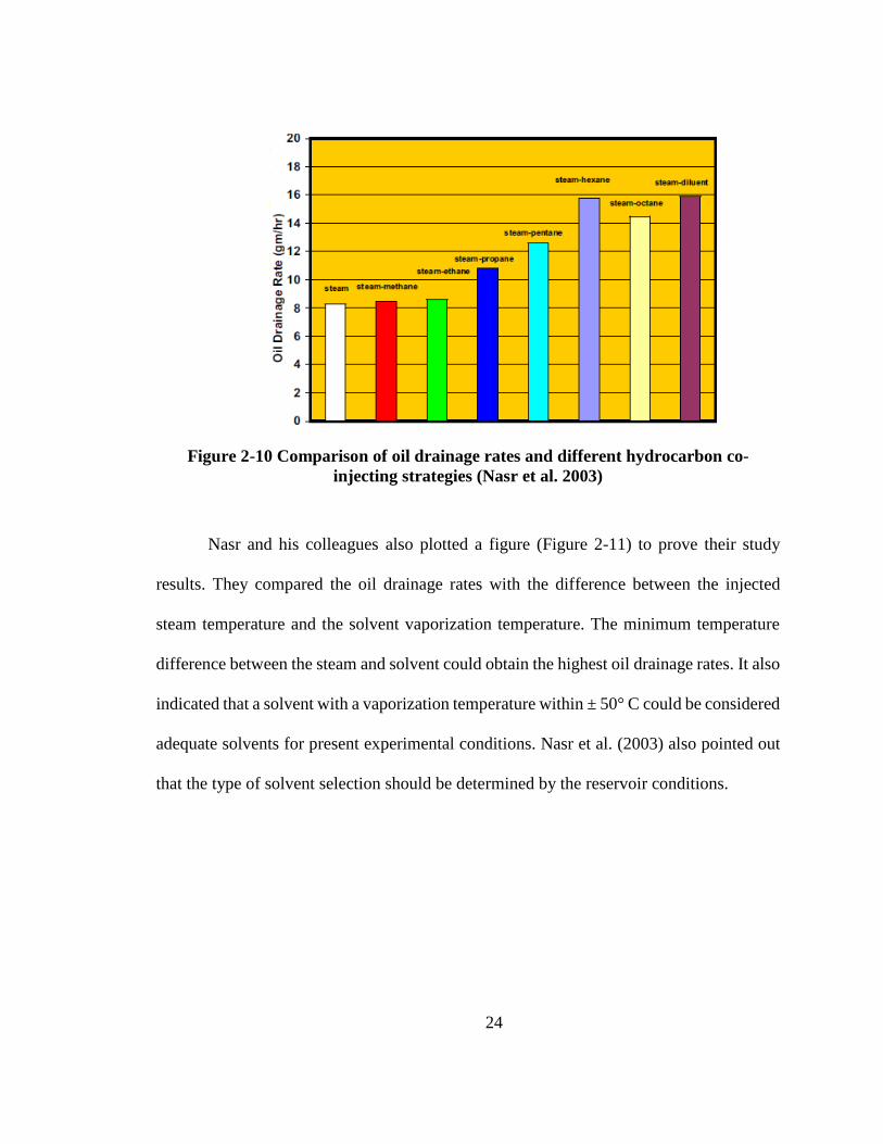
Nasr et al. (2003) conducted eight experiments in their study to investigate the
relationship between steam and solvent co-injection strategies and oil drainage rates.
Figure 2-10 illustrates the comparison of the oil drainage rates (averaged over 55 hours)
with different solvent-steam co-injection strategies. The pure-steam injection experiment
was the base case for comparing with the steam-solvent injection experiments. From left
to right, it shows that the co-injection of non-condensable components with steam such as
methane and ethane does not enhance the oil drainage rates as compared to the pure steam
injection case. On the other hand, co-injecting the condensable hydrocarbon additives (C3-
C8) or diluent (mainly C4-C10) with steam has positive effects on oil drainage rates. Hexane
and diluent obtained the highest oil drainage rates in the comparison.
Page 42
24
Figure 2-10 Comparison of oil drainage rates and different hydrocarbon co-
injecting strategies (Nasr et al. 2003)
Nasr and his colleagues also plotted a figure (Figure 2-11) to prove their study
results. They compared the oil drainage rates with the difference between the injected
steam temperature and the solvent vaporization temperature. The minimum temperature
difference between the steam and solvent could obtain the highest oil drainage rates. It also
indicated that a solvent with a vaporization temperature within ± 50° C could be considered
adequate solvents for present experimental conditions. Nasr et al. (2003) also pointed out
that the type of solvent selection should be determined by the reservoir conditions.
Page 43
25
Figure 2-11 Oil drainage rates vs. temperature difference between steam and solvent
(Nasr et al. 2003)
Nevertheless, other studies revealed that the solvent selection has converse results.
Govind et al. (2008) conducted a numerical simulation to analyze the ES-SGAD process.
They selected butane, hexane, pentane, heptane, and a mixture of C6-C8 to co-inject with
steam. They concluded that the solvent type is negligible. A comparative numerical
simulation study was done by Ardali et al. (2010); they indicated that the solvents which
were heavier than butane have the potential capabilities to enhance the oil recovery and
thermal efficiency. They also pointed out that the solvent type selection has a relationship
with bitumen properties. Butane is the best option for cold lake reservoirs and solvent
heavier than butane can improve oil recovery for Athabasca reservoirs.
Page 44
26
Effects of Solvent Concentration on ES-SAGD Process
Solvent concentration is a major parameter which has a great effect on oil
production performance in the ES-SAGD process. The effects of solvent concentration
have been studied and published in reports and the literature. Govind et al. (2008)
conducted a numerical simulation model to investigate the effect of solvent concentration
during the process. They stated that an oil production rate increases as the solvent
concentration increases. Moreover, a lower cSOR and lower temperature in a steam
chamber occur during the high concentration of solvent co-injecting with steam. Shu (1984)
proposed a correlation for heavy oil and solvent systems. Based on this correlation, a
relationship between a solvent volume fraction and viscosity of Athabasca bitumen was
plotted by Li et al. (2010). Figure 2-12 illustrates the relationship between the viscosity of
Athabasca bitumen and a volume fraction of solvent (C6) at different constant temperature.
The viscosity is decreased further with a solvent volume fraction increased when mixing
the heated bitumen at a constant temperature. The purple line, the steam temperature at 200
oC, indicates that the viscosity is decreased to 4 centipoises with a solvent volume fraction
of 0.1, while the solvent volume fraction increased to 0.3 when the viscosity of bitumen is
only 1 centipoise.
Nevertheless, the high concentration of solvent co-injected with steam has its
economical limitations because of the high price of solvent. Govind (2008) pointed out that
the optimum solvent concentration selected will be a function of solvent costs, and solvent
retention and loses in a reservoir. Akinboyewa et al. (2010) conducted a numerical
simulation of filed case studies for a bitumen reservoir. They stated that a volume of 5-10%
Page 45
27
of steam’s cold water equivalent (CWE) is adequate to enhance oil recovery and reduce
the operation cost; higher concentration will result in an uneconomical project. A numerical
evaluation of hydrocarbon additives to steam in the SAGD process was done by Mohebati
(2010). They stated that if a mole fraction of hydrocarbon additive (C6) is increasing more
than 0.01, the oil recovery factor increased slightly.
Figure 2-12 Solvent (C6) volume fraction vs. viscosity of Athabasca bitumen at
constant temperature (Li 2010)
The Impacts of Operating Pressure
Operating pressure plays an important role during the ES-SAGD process. A change
of operating pressure can affect the process performance dramatically. Mohebati et al.
(2010) conducted a simulation study to investigate the operating pressure effects on solvent
added SAGD performance. The simulation results revealed that hexane could improve the
Page 46
28
SAGD performance substantially at low steam injection pressure (1500 kPa) compared to
high steam injection pressure (1900 kPa). They pointed out that the reason for the
significant difference is due to more hexane retained in a reservoir under high injection
pressure. Ivoy et al. (2008) stated that a lower minimum producer bottom hole pressure
BHP (2200 versus 1500 kPa) enhanced the oil production rate up to 15% and reduce the
steam-oil ratio (SOR) for ES-SAGD. However, other investigations show that higher
operating pressure is more favorable for ES-SAGD. Govind (2008) stated that using butane
at higher operating pressure (4000 kPa) is optimal due to the higher vapor pressure of
butane in the simulation study.
Phase Behavior of Steam Chamber in ES-SAGD Process
The vapor-liquid phase behavior of a steam-solvent (light hydrocarbon)-bitumen
system is not uniform in a steam chamber because they have different physical properties
such as partial vapor pressure and boiling point (Li et al. 2010). They conducted an
experiment and a simulation model to investigate the phase behavior of vapor solvent,
liquid solvent, and water near the edge of the steam chamber. Based on their experiment
and simulation, they concluded that the vapor pressure dominates the properties and effects
of injected solvent and steam in the steam chamber, and partial pressure effects played an
important role for a successful ES-SAGD process. Moreover, they pointed out that
vaporized light solvent (C3) can be transported to the entire vapor-liquid interface to
dissolve in the bitumen, but may build a thick gas blanket to hinder the heat transfer. They
suggested that selecting a suitable multicomponent solvent mixture, which includes solvent
Page 47
29
in the vapor and liquid phases such as heptane and xylene, might improve the ES-SAGD
performance by changing the condensation dynamics of the solvent.
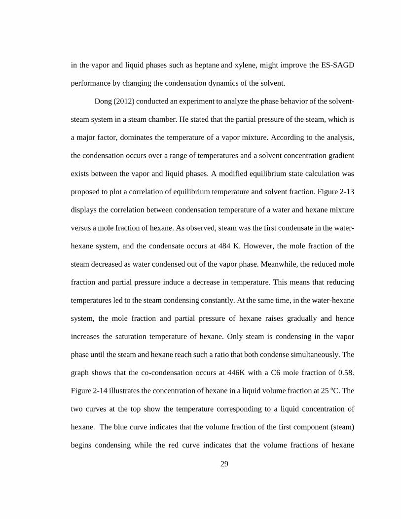
Dong (2012) conducted an experiment to analyze the phase behavior of the solvent-
steam system in a steam chamber. He stated that the partial pressure of the steam, which is
a major factor, dominates the temperature of a vapor mixture. According to the analysis,
the condensation occurs over a range of temperatures and a solvent concentration gradient
exists between the vapor and liquid phases. A modified equilibrium state calculation was
proposed to plot a correlation of equilibrium temperature and solvent fraction. Figure 2-13
displays the correlation between condensation temperature of a water and hexane mixture
versus a mole fraction of hexane. As observed, steam was the first condensate in the water-
hexane system, and the condensate occurs at 484 K. However, the mole fraction of the
steam decreased as water condensed out of the vapor phase. Meanwhile, the reduced mole
fraction and partial pressure induce a decrease in temperature. This means that reducing
temperatures led to the steam condensing constantly. At the same time, in the water-hexane
system, the mole fraction and partial pressure of hexane raises gradually and hence
increases the saturation temperature of hexane. Only steam is condensing in the vapor
phase until the steam and hexane reach such a ratio that both condense simultaneously. The
graph shows that the co-condensation occurs at 446K with a C6 mole fraction of 0.58.
Figure 2-14 illustrates the concentration of hexane in a liquid volume fraction at 25 oC. The
two curves at the top show the temperature corresponding to a liquid concentration of
hexane. The blue curve indicates that the volume fraction of the first component (steam)
begins condensing while the red curve indicates that the volume fractions of hexane
Page 48
30
condenses first. The blue line indicates that the temperature of both steam and hexane has
condensed to the liquid phase completely. Dong (2012) also pointed out that the phase
behavior of the solvent-steam system in a steam chamber is sensitive to the number of
hydrocarbons. As the number of hydrocarbon increases, the solvent concentration for
solvent condensation decreases. The pressure in the steam chamber has little effect on the
phase behavior. The temperature difference between the SAGD and the ES-SAGD
processes are shown in Figure 2-15. The temperature difference is 40 oC lower than SAGD
compared with ES-SAGD.
Figure 2-13 Correlation between condensation temperature of water and hexane
mixture versus mole fraction of hexane at 2000 kPa (Dong 2012)
Page 49
31
Figure 2-14 Correlation between condensation temperature of water and hexane
mixture versus volume fraction of hexane at 2000 kPa (calculated at 25 oC) (Dong
2012)
Figure 2-15 Temperature profiles in distance at the edge of steam chamber between
SAGD and ES-SAGD (More Fraction of Hexane at 0.01, 2000 kPa) (Dong 2012)
Page 50
32
The Impacts of Reservoir Heterogeneities
As aforementioned, the growth of a steam chamber is the most important for the
SAGD process. The description of the steam chamber is always assumed to be in a
homogenous, isotropic reservoir. In practice, no reservoir is homogenous and isotropic
because of natural geological features such as shale layers, water zones, and gas caps. Many
oil companies have reported the existence of shale layers and water zones in their projects
such as Long Lake (Nexen), Firebag (Suncor), and Surmont (ConocoPhillips) (Xu 2015,
Bao 2012). Therefore, an accurate prediction of SAGD performance for field-type systems
could not be achieved without a comprehensive understanding of reservoir heterogeneities
(Chen et al. 2008). Several researchers have been investigating the effects of reservoir
heterogeneities on steam chamber development in the SAGD process for several decades.
Laboratory-scale experiments and reservoir simulations are the main approaches for
investigating reservoir heterogeneities.
Yang and Butler (1992) conducted a series of experiments to investigate the effects
of heterogeneities for the SAGD process. They used a two-dimensional sand-packed model
to mimic two reservoir types: reservoirs with thin shale layers and reservoirs with
horizontal layers of different permeability. There were two scenarios in a reservoir with
two layers, one was a high/low permeability reservoir, and another was a low/high
permeability reservoir. They stated that the SAGD performance of a high/low permeability
reservoir was similar with that of a high permeability reservoir. For a low/high permeability
reservoir, they found an undermining of steam in the low layer (high permeability), and the
effect was reduced with time. Furthermore, they carried out a comparison of cumulative
Page 51
33
oil production from the previous setup with all low permeability setup and found little
difference. They noticed that underlying steam improved the gravity drainage rate over the
interlayer surface. Adversely, the viscosity of a production fluid increased due to a higher
oil/water emulsion appearing over the underlying steam. For the experiments of a reservoir
with shale layers, they concluded that short horizontal barriers had no effect on production
performance. On the other hand, long horizontal barriers reduce the production rate
dramatically. In addition, they investigated the reservoir dipping effect for a low/high
permeability setup. They noticed that a high production performance was obtained from
the reservoir dipping upward compared to the reservoir dipping downward. They reasoned
that the production rates are dominated by the total drainage height. Thus, they pointed out
that a maximum production rate would be obtained by placing the production well at the
lowest location of a dip reservoir. Yang and Butler (1992) also pointed out that the presence
of long shale layers in a reservoir could cause various advancement velocity at the upper
and lower interface of the shale layers. This phenomenon is decreased by the steam and
heated bitumen conducted over the shale layers. Nasr et al. (2003) conducted an experiment
model by using an element approach to study the impacts of gas cap and top water on
SAGD performance at Alberta Research Council (ARC). They stated that the steam moved
into both gas cap and top water zones and more steam penetrated water zone than that of
gas cap. For the top water case, more initial oil in place has been produced compared to
the gas cap case. However, the experimental analyses have limitations such as time
consuming, accuracy, and design. These difficulties have been partially overcome by using
a numerical simulation method (Chen 2008, Wang 2015).
Page 52
34
Numerous numerical simulation studies have investigated the impacts of reservoir
heterogeneities on the SAGD process (Law 2003, Chen 2008, and Xu 2014). Pooladi-
Darvish and Mattar (2002) conducted a simulation mode which contains a gas cap and top
water to examine the effects of shale layers’ continuity in a vertical direction on the SAGD
process. They observed only a minor effect on production performance. Law et al. (2003)
studied a simulation model with the existence of confined and unconfined top water. They
investigated the impacts of initial pressure and injection pressure on the SAGD process.
The results indicated that as the pressure difference in a steam chamber increased, a top
water zone decreased in production performance. Chen et al. (2008) carried out a numerical
simulation to investigate stochastic distribution of shale barriers near a well region and
above a well region. They concluded that short shale barriers, which are located near the
well region, impaired the vertical permeability and hampered the vertical growth of the
steam chamber. For the above well region case, the shale barriers affect both the vertical
and horizontal growth of the steam chamber. A numerical study was done by Xu et al.
(2014, 2017) to investigate impacts of lean zones on SAGD performance. They located the
lean zones above the injector, between the injector and producer, and below the producer.
They stated that the location of lean zones has a most important effect on SAGD
performance. The lean zones located above the injector severely influenced the
performance, and the lean zones located below the producer yielded a little impact. They
also conducted a sensitivity analysis of lean zones, which is related to vertical distribution,
horizontal spacing, and sizes. They indicated that increasing the sizes and reducing the
interval distance of the lean zones could influence the SAGD performance significantly.
Page 53
35
Wang et al. (2015) conducted a comprehensive analysis for lean zones and shale
distribution. The results showed that significant heat lost in the lean zones caused a higher
cumulative steam-oil ratio. They pointed out that the lean zone beneath the producer will
not affect the SAGD performance. This conclusion is consistent with the results of Xu
(2014). A three-dimensional geological model which contains top water and gas cap zones
(thief zones) for a Surmont pilot was constructed by Bao et al. (2011). They utilized a
geological model to investigate the effects of top water and gas cap zones on both SAGD
and ES-SAGD. The results indicated that the production performance of the SAGD process
is more sensitive to injection pressure. The high injection pressure led to early steam
breakthrough into the water zone causing top water flows into steam chamber. For the ES-
SAGD process, they selected a hydrocarbon mixture (which ranges from C4-C11) to inject
with steam. They found that the steam chamber grows more transversely compared to the
SAGD case.
Page 54
36
RESERVOIR MODEL
Reservoir simulation is a major method to eveluate the SAGD and ES-SAGD
processes. In this study, we generate a homogenous simulation model with the presence of
lean zones to investigate the production peroformance of the SAGD and ES-SAGD
processes. The CMG STARS (2015 version) simulator is used to build the homogenous
model and study the mechanisms of these processes. The parameters of the reservoir model
come from published papers for the McMurray Formation in northeast Alberta .
Basic Model Construction and Description
The resevoir is a three-dimensional, rectangular, homogenous model with a single
well pair. The lean zone layers are mobile water zones and placed into the reservoir model
before the SAGD and ES-SAGD proceses. The lean zones are placed above the injection
well. The number of lean zone layers range from 1 to 20 with an even number order. The
thickness of each lean zone layer is 0.5m. The simulations will be run for 15 years to
investigate the impacts of lean zones on the SAGD and ES-SAGD processes.
Grid System
A homogenous simulation model is established by CMG STARS software. The
dimensions of the reservoir model are 100x50x40m. It is divided into 8,000 blocks with
100x1x80 blocks in the i, j, and k directions. The dimensions of each block are 1x50x0.5m
in the i, j, and k directions. Figure 3-1 illustrates generation of a right half two-dimensional
Page 55
37
simulation model in the i-k directions. Figure 3-2 displays a three-dimensional right half
reservoir model.
Figure 3-1 Grid structure of a right half reservoir model in i-k directions
I
njector
Producer
Producer
Injector
Injector
Page 56
38
Figure 3-2 A right half reservoir model in 3D view
The producer and injector are placed at the bottom left corner with 50m length in
the j direction. The injector is 5 meters above and parallel to the producer. The producer is
located 5 meters above the reservoir base. The perforation of the injector is located at the
block of (1, 1, 59), and the producer is located at the block of (1, 1, 69). The SAGD and
ES-SAGD processes have the same input parameters except for solvent injected with steam
in the ES-SAGD process.
Injector
Producer
Page 57
39
Reservoir Properties
The input parameters for this reservoir model are listed in Table 3-1. These
parameters are from the McMurray Formation in northeast Alberta. Figures 3-3 and 3-4
display oil-water relative permeability and gas-liquid relative permeability, respectively.
Table 3-1 Reservoir parameters for simulation model
Parameters Valus
Reference Depth, 𝑚 230
Reference Pressure, 𝑘𝑃𝑎 1050
Reference Temperature, ℃ 7
Porosity 0.307
Permeability (horizontal), 𝑚𝐷 6292
Permeability (vertical), 𝑚𝐷 4892
Connate Water Saturation 0.25
Initial Oil Saturation 0.75
Formation Heat Capacity 𝐽/𝑚3℃ 2.3E+06
Reservoir Rock Thermal Conductivity 𝐽/𝑚 𝐷𝑎𝑦 ℃ 2.7E+5
Water Phase Thermal Conductivity 𝐽/𝑚 𝐷𝑎𝑦 ℃ 5.4E+4
Oil Phase Thermal Conductivity 𝐽/𝑚𝐷𝑎𝑦 ℃ 1.2E+4
Formation Compressbility Conductivity 1/𝑘𝑃𝑎 1.0E-6
Overburden/underburden Volumetric Heat Capcity 𝐽/𝑚 ℃ 𝐷𝑎𝑦 2.3E+6
Overburden/underberden Thermal Conductivity 𝐽/𝑚3 ℃ 1.5E+5
Page 58
40
𝒌𝒓𝒘 𝒌𝒓𝒐
Figure 3-3 Water–oil relative permeabilility,
𝒌𝒓𝒘 is the water-phase permeability, and 𝒌𝒓𝒐 is the oil-phase permeability
𝒌𝒓𝒈 𝒌𝒓𝒍
Figure 3-4 Gas-liquid relative permeability,
𝒌𝒓𝒈 is the gas-phase permeability, and 𝒌𝒓𝒍 is the liquid-phase permeability
Page 59
41
Fluid Properties
The critical bitumen properties are characterized by CMG WinProp. The
composition of bitumen contains 0.082 mole fraction of methane and 0.918 mole fraction
of heavy components. The correlation of bitumen vicosity and temperature is shown in
Figure 3-5. As observed, the viscosity of bitumen is more than 1 million centipoises at
reservoir temperature of 7 oC. However, when the temperature is up to 200 oC, which is
the temperature at the edge of a steam chamber, the viscosity reduces to about 10
centipoises.
Figure 3-5 The correlation of temperature versus bitumen viscosity
Page 60
42
Operation Parameters for Cases
The steam is injected at the temperature of 223 oC. The quality of the steam is 0.9.
The constraints of the injector are a maximum surface water rate (STW) with 30 m3 /day
in cold water equivalents (CWE) and the maximum bottom hole pressure (BHP) with 2500
kPa; the producer is constrained to a maximum liquid rate at 30 m3 /day. For the
initialization of the SAGD process, the injection and production wells need to be preheated
before bitumen is produced. The period of preheating is 90 days.
The Location of Lean Zones in the Reservoir Model
Earlier numerical moddelling by Xu et al. (2014) indicates that the location of lean
zones in a reservoir has different effects on the SAGD performance. The lean zones, which
are located above the well pair, have significant effects on the SAGD performance. The
modelling results also indicate that the sizes of the lean zones also affect the performance
severely on SAGD. Therefore, in this study, the lean zones are placed above the injection
well to analyze how the lean zones affect both SAGD and ES-SAGD performance.
Page 61
43
DISCUSSION OF SAGD PROCESS WITH LEAN ZONES
Introduction
The investigation of the SAGD process with no-lean zone (base case) and lean
zones models will be compared in different aspects. Moreover, the sensitivity analysis of
lean zones will be illustrated in this chapter. In addition, this study is a reference case to
compare the SAGD process with the ES-SAGD process.
The Comparison of Base Case and Lean Zones (2 meters) Case
In this chapter, the lean zone layers with 2 meters’ thickness are created in the base
model. Figure 4-1 displays the location of the lean zone layers in an i-k 2D cross-section.
The connate water saturation of this model is 0.25. The water saturation of the lean zones
is 0.7, and they are 14 meters above the injector.
Figure 4-1Water saturation profile in cross-section of SAGD
Sw
Page 62
44
Analysis and Comparison of the Steam Chamber
The mechanisms and analyses of a steam chamber have been investigated by many
researchers. Experimental and simulation methods are the two main methods to describe a
steam chamber in the SAGD process (Bulter1988, Sasaki 1999, Ardali 2010, and Ji 2014).
In this study, a numerical simulation method is used to study the effects of lean zone in the
SAGD process. For a better understanding of the mechanisms of the steam chamber, we
divided the reservoir into four zones in the i-k 2D cross-section according to the variations
of properties distribution of the reservoir. The analytical properties are temperature, gas
saturation, oil saturation, oil mobility, and water saturation. Figure 4-2 shows the
temperature distribution profiles with the four zones for the two cases, respectively. The
dashed line of the base case is curve of the analytical properties from the inner steam
chamber to the cold oil sand (left to right sides) in the i-k direction. Figure 4-3 illustrates
the variations of the temperature, gas saturation, oil saturation, water saturation, and oil
mobility along the line of study which is in the base case of Figure 4-2.
Zone A is called the steam zone where it is filled by steam, residual oil, and connate
water. The temperature is constant, and gas saturation maintains in a high level.
Zone B is called the steam condensation zone where the steam contacts with the
bitumen and reservoir rock. In this zone, the latent heat of the steam transfers into the
bitumen and the resevoir rock due to a temperature difference. As a result, the steam is
condensed in this zone. Heat conduction plays a dominant role in the heat transfer process.
As seen in Figure 4-3, the temperature begins to decrease, the gas saturation drops down
Page 63
45
to zero because of the condensed steam, and the water saturation and oil saturation
increased rapidly. Hence, there is a dramatic increase in the oil mobility.
Zone C is called the mobile oil zone. The viscosity of heated bitumen has reduced
dramtically and become flowable. Subsequently, mobilized oil is drained downward to the
producer by gravity. The oil saturation stays in high level and the water saturation drops
slowly. The oil mobility decreases as the temperature is continuing to decrease.
Zone D is called the immobile oil zone. The tempature of bitumen in this zone is
not affected sufficiently by the heat of steam. The bitumen remains in its original state. All
of the analytical properties do not change in this zone.
As observed in Figure 4-4, the steam chambers are quite different between the two
cases, especially in the middle of the steam chamber. To compare and analyze the steam
chamber in detail, we also divided the steam chamber into three areas from the bottom to
the top of the reservoir in the vertical direction.
Base case Lean zones case
Figure 4-2 Comparison of the temperature distributions with different zones of
SAGD process with 2500 kPa injection pressure at 273 days
T (oC )
Page 64
46
Base case
Figure 4-3 Schematic presentation of the temperature, gas saturation, oil saturation,
oil mobility, water saturation profiles along the line of study (50-67 m) in SAGD
process with 2500 kPa injection pressure at 273 days
Base case Lean zones case
Figure 4-4 Comparison of the temperature profiles with three areas of the reservoir
in SAGD with 2500 kPa injection pressure at 273 days
T (oC )
Page 65
47
4.2.1.1 Bottom Area of the Reservoir
The comparitive analysis at the bottom area of the reservoir has been done through
the steam chamber profiles and property variations along the line of study. Figure 4-5
displays the temperature profiles at the bottom area of the reservoir at 273 days with the
base case and lean zone case. Figure 4-6 shows the variations of the analytical properties
(gas saturation, oil saturation, oil mobility, water saturation, temperature) at 273 days along
the study line.
As seen from Figures 4-5 and 4-6, zone A is the steam zone which is also called the
non-condensation zone. The intervals of the steam zones for both cases are 1.0 m. The
analytical parameters are constant in the steam zones. The temperature, gas saturation
(mainly steam), oil saturation, oil phase mobility, and water saturation are 223 oC, 0.54,
0.30, 17.05 md/cp, and 0.17 for both cases, respectively. The gas saturation fluctuates
slightly but remains in saturation conditions. There is no oil fluid flow as the oil saturation
and oil phase mobility are quite low. In this zone, the pores of the reservoir are filled with
steam, residue oil, and water.
Zone B is the condensation zone (1.0m for both cases). The steam condensed at the
vapor-liquid interface once the reservoir conditions were insufficient to the saturated steam
conditions (Butler et al. 1998). The five physical properties have been varied along the line
of study.
First, the gas saturation (mainly steam) decreased sharply from 0.53 to zero in this
region. Second, the temperature begins to drop as well. On the other hand, the oil saturation,
oil phase mobility, and water saturation increased dramatically for both cases. Third, the
Page 66
48
peak of oil saturation in this region is 0.63 for the base case and 0.72 for the lean zone case.
Moreover, as the latent heat of steam is conducting into the oil phase, the oil phase mobility
is also increased significantly in both cases. The highest values are 158 md/cp for the base
cases and 253 md/cp for the lean zones case. In addition, the water saturations increase
because of the steam condensation in this region. The peaks of water saturation are 0.41
and 0.28 for both cases. It indicates that more steam has condensed in this zone for the base
case. To compare the two cases, the oil saturation in the base case is lower than that in the
lean zone case while the water saturation in the base case is higher than that in the lean
zone case. It illustrates that most heat of the steam in the lean zone case is released at the
right boundary of zone B. Therefore, the oil phase mobility in the lean zone case is higher
than that in the base case.
Zone C is the mobile oil region (4.8 m and 3.0 m). The viscosity of the bitumen has
been reduced enough to flow since the latent heat of steam was conducted into this region
continuously. The mobilized oil is drained to the producer by gravity. The gas saturations
in both cases remain at zero. The decreased rate of temperature is quicker as compared to
the other regions. Oil saturation continues to rise while the water saturation starts to drop
as the heat of steam is transmitted transversely. The oil mobility in the base case reached
the highest value, while the lean zone case decreases sharply. There are several contrasting
observations in the two cases. First, the temperature interval is different. As the oil phase
mobility drops to zero, the temperature in the lean zone case is 94.5 oC contrasted with 70.9
oC in the base case. Moreover, the mobile oil zone in the base case (4.6 m) is larger than
that in the lean zone case (3.0 m). Third, the peak of the oil phase mobility in the base case
Page 67
49
is in the mobile oil zone; however, the peak value is between the interface of zone B and
zone C in the lean zone case. Thus, the efficiency of heat conduction in the base case is
higher than that in the lean zone case.
Zone D is the immobilized oil zone (after 56.75 meters in the base case and 55.25
meters in the lean zone case). The five observed properties of the bitumen and reservoir
have not changed due to the absence of heat conducting into this zone. All five properties
remain in the original reservoir conditions.
Base case Lean zone case
Figure 4-5 Comparison of the temperature profiles at bottom area of the reservoir
with 2500 kPa injection pressure at 273 days. The dashed line indicates the location
of study line
T (oC )
Page 68
50
Base case (No-lean zone)
Lean zone case
Figure 4-6 Schematic representation of the temperature, gas saturation, oil saturation,
oil mobility, water saturation profiles along the line of study (50-65 m) in SAGD
process with 2500 kPa injection pressure at 273 days
Page 69
51
4.2.1.2 Middle Area of the Reservoir
A similar analysis has been carried out in the middle area of the reservoir for both
cases. Figure 4-7 illustrates the comparison of the temperature profiles at the middle of the
reservoir at 273 days. Figure 4-8 shows the temperature, gas saturation, oil saturation, oil
mobility, and water saturation profiles along the dashed line (50-65 m) in the SAGD
process at 273 days. There are significant differences in the middle of the reservoir because
the lean zones are in this region. As observed from Figure 4-7, in the lean zone case, the
latent heat of steam is thieved into the lean zones extensively through all of four zones. As
a result, the temperature profile is in a convex shape.
Zone A (1.5m and 1.25m for the two cases) is the non-condensation zone. The
steam chamber remains in the saturated conditions. The properties are constant in the steam
zones. The temperature, oil saturation, oil phase mobility, and water saturation are stable.
There is no oil fluid flow but the live steam. The pores of the reservoir contain steam,
residue oil and connate water.
Zone B (0.75m in the base case and 1.0m in the lean zone case) is a steam
condensation zone. Since the latent heat of steam releases into the bitumen, the steam
condensation occurs in this region. The gas saturation decreased sharply from 0.49 to zero
due to the decreasing temperature. In contrast, the oil saturation, oil phase mobility, and
water saturation increased dramatically in the two cases. This scenario is similar to the
bottom of the reservoir. The peak of oil saturation in this region is 0.67 in the base case,
and 0.70 in the lean zone case. As quickly as oil saturation has increased, the oil phase
mobility has also increased significantly in both cases. The highest values in both cases are
Page 70
52
265 md/cp in the base case and 261 md/cp in the lean zones case. These values are observed
near the interface of zone B and zone C. The water saturations increase because of the
condensation. The peaks of water saturation are 0.34 and 0.30 in both cases, respectively.
Zone C (4.75m in both cases) is the mobile oil zone. The bitumen has been able to
flow due to viscosity conduction. The gas saturations in both cases are almost zero. The
temperature drops significantly in this region. Oil saturation continues to rise while the
water saturation starts to drop as the heat of steam is delivered transversely. The oil phase
mobility decreases as the distance increases from the steam chamber. As seen, the
decreasing rate of the temperature is different in the two cases. As the oil phase mobility
drops to zero, the temperature in the lean zone case is 100 oC compared to 57.8 oC in the
base case. It indicates that the heat of steam is losing into the lean zones.
Zone D is the immobilized oil zone (after 57.0 m). The latent heat of steam has not
been conducted into this region effectively. The reservoir properties have been restored to
the original conditions.
Base case Lean zone case
Figure 4-7 Comparison of the temperature profiles at middle area of the reservoir in
SAGD with 2500 kPa injection pressure at 273 days. The dashed line indicates the
location of study line
T (oC )
Page 71
53
Base case (No-lean zone)
Lean zone case
Figure 4-8 Schematic representation of the temperature, gas saturation, oil saturation,
oil mobility, water saturation profiles along the line of study (50-65m) in SAGD
process with 2500 kPa injection pressure at 273 days
Page 72
54
4.2.1.3 Top Area of the Reservoir
A similar comparative analysis has been done at the top part of the reservoir. Figure
4-9 shows the temperature profiles at the top area of the reservoir in the SAGD process at
273 days in the two cases. Figure 4-10 displays the schematic representations of the
temperature, gas saturation, oil saturation, oil mobility, and water saturation profiles along
the dashed line (50-65 m) in the SAGD process at the same time. As observed from Figure
4-9, zone B is of partial existence in this region because the growth of the steam chamber
develops to sideways once the steam has contacted the overburden (Butler et al. 1998).
Figure 4-10 displays the variations of gas, oil, and water saturations, temperature and oil
phase mobility at the top part of the reservoir.
Zone A is the non-condensation zone (3.0m and 3.25m). The temperature and
pressure are almost constant. The other properties are almost constant in the steam zones.
The temperature, gas saturation (mainly steam), oil saturation, oil phase mobility, and
water saturation are constant. The pores of the reservoir are mainly filled with steam. The
gas saturation is 0.54 in the base case and 0.58 in the lean zone case. It is consistent with
Wang et al. (2015). They found that a part of mobile water in lean zones was vaporized
into the steam zone and condensed with the injected steam at the edge of the vaper-liquid
phases.
Zone B (1.25m in the base case and 1.0m in the lean zone case) is a steam
condensation zone. Since the steam just begins condensing in this area, zone B is pinching
out at the upper part of the area. The gas saturation decreases sharply. The temperature
Page 73
55
starts to reduce. However, the oil saturation, oil phase mobility, and water saturation
slightly rise in both cases. The water saturation increases because of the condensation.
Zone C is the mobile oil zone (2.75m in both cases). The bitumen has been
mobilized by the heat. The mobilized bitumen is drained towards the producer by gravity.
As seen in Figure 4-10, the gas saturations in both cases remain near zero. The temperature
declines due to the loss of heat. Oil saturation continues to increase when the water
saturation begins to drop as the thermal energy of the steam is conducted sideways. The oil
phase mobility reached the peak values in the two cases. It is 175 md/cp in the base case
and 102 md/cp in the lean zone case. The temperature decreasing rate is also different in
the two cases. When the oil phase mobility is zero, the corresponding temperature in the
lean zone case is 82.6 oC compared to 71.7 oC in the base case. The phenomena indicates
that the heat of steam is conducted into the lean zones more effectively.
Zone D is the immobilized oil zone. The temperature is still low so that bitumen
cannot be heated to flow. The reservoir condition remains in its original state.
Base case Lean zone case
Figure 4-9 Comparison of the temperature profiles at top area of the reservoir in
SAGD process with 2500 kPa injection pressure at 273 days. The dashed line indicates
the location of the line of study.
T (oC )
Page 74
56
Base case
Lean zone case
Figure 4-10 Schematic representation of the temperature, gas saturation, oil
saturation, oil mobility, water saturation profiles along the line of study (50-65 m) in
SAGD with 2500 kPa injection pressure at 273 days
Page 75
57
Comparative Analysis on the Impacts of Lean Zones in the reservoir
4.2.2.1 Water Saturation and Velocity Vector of Water Distribution
The water saturation distribution and velocity vector of water in the two cases are
shown in Figure 4-11. The direction of all velocity vectors of water is towards the producer
in the base case. On the other hand, the water not only flows to the producer but also flows
into the lean zones. This further indicates that the latent heat of steam has lost into the lean
zones. Xiu et al. (2014) stated that the lean zones were the priority pathways for the steam
because of higher mobility and heat conductivity compared to the bitumen. Due to the high
mobility of water, the mobile water also increased the convective heat flux in the lean zones.
These will lead to high consumption of steam to be injected. They also pointed out that the
mobile water in the lean zones was produced with the condensed water from the producer.
The water saturation variations in the lean zones indicate that the mobile water in the lean
zones flowed into the steam chamber. Meanwhile, the void pores are filled with the steam
causing more steam consumption in the steam zone.
Page 76
58
Figure 4-11 Comparison of water saturation and water velocity vector in SAGD with
2500 kPa injection pressure at 273 days.
Base case
Lean zone case
Page 77
59
4.2.2.2 Production Variations in the Steam Chamber
As seen from Figure 4-12, the steam chamber in the lean zone case is slightly bigger
than that in the base case. It illustrates that the mobile water, which is in the lean zones, is
produced with condensed water. It is because part of the mobile water was vaporized and
condensed with the steam coincidentally. Figure 4-13 shows the comparison of cumulative
water production. It is obvious that the lean zone case produced more water from the
reservoir than the base case. On the other hand, it can be seen from Figure 4-14 that since
the lean zone case produced more water than the base case, the oil recovery in the lean
zones case is less than in the base case.
Figure 4-12 Comparison of the seam chamber volume
15710 15720 15730 15740 15750 15760 15770 15780
Base case
Lean zones case
Steam chamber volume, m3
Page 78
60
Figure 4-13 Comparison of the cumulative water production
Figure 4-14 Comparison of the oil recovery factor
66200 66400 66600 66800 67000 67200 67400
Base case
Lean zones case
Cumulative water production, m3
60.6 60.8 61 61.2 61.4 61.6 61.8 62 62.2 62.4 62.6
Base case
Lean zones case
Oil Recovery Factor, %
Page 79
61
Comparison and Analysis of the Growth of the Steam Chamber
The growth of the steam chamber in both cases is described with the essential
reservoir properties such as gas and temperature profiles in the i-k cross section with 2500
kPa injection pressure at 180, 365, and 730 days. With reference to Figures 4-15 to 4-16,
the steam chamber grows upward as the steam is injected into the reservoir.
After the steam reached the overburden, the growth of the steam chamber expands
sideways along the overburden. As seen from these figures, the steam chamber developed
uniformly in the base case. On the other hand, in the temperature profiles, the steam
chamber has a convex shape when it contacts with the lean zones at 180 and 365 days.
According to Figure 4-16 the gas saturation distribution did not become convex in the lean
zone region. However, the steam zone in the base case is lager than that in the lean zone
case at 180 days. After 730 days, the shape of the steam chamber was not affected by the
lean zones and its shape and area are almost the same.
Page 80
62
Base case Lean zone case
Figure 4-15 Comparison of the temperature profiles in cross section of SAGD with
2500 kPa injection pressure at 180 days, 365 days, and 730 days
180 days
365 days
730 days
Page 81
63
Base case Lean zone case
Figure 4-16 Comparison of the gas saturation profiles in cross section of SAGD with
2500 kPa injection pressure at 180 days, 365 days, and 730 days.
180 days
365 days
730 days
Page 82
64
Sensitivity Analysis of Reservoir with Lean Zones in SAGD Process
In this section, we investigated the effects of thickness and water saturation of the
lean zones on the SAGD process. Moreover, the vertical and horizontal permeability
variations were introduced into the model to study the effects of reservoir heterogeneity in
the SAGD process.
According to Figure 4-17, the layers of a lean zone were increased gradually from
0 to 20 layers (from 0 to 10 meters). As observed in this figure, as the thickness of a lean
zone increased, the oil recovery factor decreased. It proved that the thickness of a lean zone
has a significant impact on the SAGD performance.
The effects of water saturation on the performance in the lean zones are shown in
Figure 4-18. The water saturation in the lean zones is set from 0.60 to 0.95 with an interval
of 0.05. As we observed, the oil recovery rate is reduced as the water saturation in the lean
zones increased. The higher water saturation in the lean zones impairs the oil production
of the SAGD process because more water is produced from the lean zones.
Figure 4-19 illustrates the effect of vertical permeability on the SAGD process. The
ratio of vertical permeability with horizontal permeability has a different effect on the
SAGD performance. The ratio was set from 0.25 to 1.5. As the ratio increased, the oil
recovery begins to drop; when the vertical permeability is 0.75 times the horizontal
permeability, the oil recovery factor reaches the lowest value. However, as the ratio
continues to rise, the oil recovery rate increases to a higher value. The low vertical
permeability led to the lateral growth of the steam chamber. Even though the growth rate
Page 83
65
of the steam chamber is reduced, the steam chamber is larger than in the normal case.
Therefore, the vertical permeability severely affects the SAGD performance.
Figure 4-17 Comparison of the oil recovery factor vs. thickness of the lean
zones
Figure 4-18 Effects of the lean zone water saturation vs. the oil recovery factor
55
56
57
58
59
60
61
62
63
0 5 10 15 20 25
Oil
reco
vry
fact
or,
%
Number of lean zone layers
60.4
60.6
60.8
61
61.2
61.4
61.6
0.5 0.6 0.7 0.8 0.9 1
Oil
reco
very
fac
tor,
%
Water saturation of the lean zones
Page 84
66
Figure 4-19 Effects of the ratio of vertical and horizontal permeabilty vs. the
oil recovery factor
Conclusions of the SAGD Process
The impacts of lean zones on the SAGD process have been investigated by
comparing their bottom, middle, and top locations in a reservoir. The analyses of
temperature, gas saturation, water saturation, oil satuation, and oil mobility variations in
the SAGD process have been concluded. The presence of lean zones in the reservoir
impaired the steam chamber significantly because of the heat loss into the lean zones.
Steam consumption increased because the mobile water was produced with condensed
steam to form a larger steam chamber than those in no-lean zone reservoirs. Because of
this, higher water production led to an increased operation cost.
61.1
61.2
61.3
61.4
61.5
61.6
61.7
61.8
0 0.2 0.4 0.6 0.8 1 1.2 1.4 1.6
Oil
reco
very
fac
tor,
%
Ratio of vertical and horizontal permeability
Page 85
67
Sensitivity analyses have been conducted to investigate the effects of lean zones on
the SAGD process. First of all, the thickness of the lean zones was studied in the SAGD
process. As the thickness of lean zones increased, the oil production continued to drop.
Second, the water saturation in the lean zones impairs the oil produciton of the SAGD
process. Third, lower vertical permeability in the reservoir with lean zones has effects on
the SAGD performance. The lowest oil production occurred when the ratio of vertical and
horizotal permeability was 0.75.
In conclusion, the existence of lean zones in an oil sand reservoir severely impaired
the SAGD performance. To improve the oil recovery in the reservoir with lean zones, the
ES-SAGD method will be introduced in the coming chapter.
Page 86
68
ANALYSIS OF ES-SAGD PROCESS WITH LEAN ZONES
Introduction
ES-SAGD is a process in which the hydrocarbon additives (solvent) are co-injected
with steam into oil sands reservoirs to reduce the bitumen viscosity at the edge of a steam
chamber thus improving oil mobility and oil recovery (Easr. 2003). Some reserchers also
indicated that ES-SAGD decreases the steam consumption and greenhouse gases emission.
In this chapter, the ES-SAGD process is conducted in the model to investigate the impacts
on a reservoir with lean zones.
Solvent Characterization
Many solvents are typically not pure components due to a high price. In practice, a
blend of various light hydrocarbon components (a hydrocarbon mixture) is used as an
injecting solvent. In this study, a selection of hydrocarbon mixture (C4 to C11) was
characterized by using CMG software (WinProp 2015 version) to match the phase
behavior of the additives at resevoir conditions. Furthermore, the components of the
hydrocarbon mixtures have been lumped into three pseudo-components which match the
liquid density and saturation pressure based on experimental data. After charaterization,
the data was exported into STARS for the ES-SAGD simulation.
The equilibrium K-value calculation in the STARS simulator uses a two-phase
equilibrium description fluid model. Liquid viscosities are inputted as tables which are
referenced as temperature and pressure. The defaults non-linear mixing rule was used to
determine both the oleic and water phases viscosities.
Page 87
69
Solvent Injection Strategies
The hydrocarbon additives (a solvent mixture) are co-injected with the steam. It
contains 66.63% mole fraction of IC4-NC5, 31.06% mole fraction of C6-C8, and 2.31%
mole fraction of C9-C11. Solvent is co-injected with steam continuously at a 10% weight
fraction. The injection period is 15 years.
Comparison of Base Case and Lean Zone Case
A similar analysis as discussed in the previous chapter for SAGD is for the ES-
SAGD process to investigate the effects of solvent in resevoirs with lean zones. Figure 5-
1 displays the comparison of temperature profiles in the base case and the lean zone case
in the ES-SAGD process. The steam chambers in the two cases are significantly different
due to the presence of lean zones. The growth of the steam chamber in the base case
develops more transversely due to the hydrocarbon additives (solvent). In the lean zone
case, it is obvious that the shape of the steam chamber is affected by the lean zones severely.
The steam chamber is formed in a concave shape in the lean zone area. Figure 5-2 shows
the variations of the analytical properties along the line of study which is shown in Figure
5-1 in the base case. The distributions of the hydrocarbon additives (in three pseudo-
components) and steam mole fraction are shown in Figure 5-3. The reservoir is divided
into four zones according to the property variations. The description of the divided four
zones is as follows:
Page 88
70
Non-condensation zone A: The pores of rock are filled with steam, solvent, residual
oil and water. Since the steam and solvent are in saturation conditions, there is no
condensation occurring. The temperature and pressure remain constant.
Condensation zone B: The steam and solvent start to condense once the vapor
contacts with the sorrounding bitumen and reservoir rock. The latent heat of steam transfers
to the cold oil. The solvent begins to dissolve the bitumen to further reduce the viscosity.
Bitumen mobilized zone C: Due to the heat conduction and solvent dissolution, the
bitumen is mobilized and drains to the producer by gravity.
Immobilized zone D: As this zone is beyond the steam chamber, the reservoir is in
original reservoir conditions.
As we have done in Chapter Four, the bottom, middle, and top of the reservoir are
selected in order to compare and analyze the differences of the steam chamber in the two
cases. Figure 5-4 illustrates the comparison of the steam chamber in the three locations in
the ES-SAGD process in the two cases.
Base case Lean zone case
Figure 5-1 Comparison of the temperature profiles with different zones of ES-SAGD
process with 2500 kPa injection pressure at 273 days. The dished line is the study line
T (oC )
Page 89
71
Figure 5-2 Schematic representation of the temperature, gas saturation, oil saturation,
oil mobility, water saturation profiles along the line of study (50-65 m) in ES-SAGD
process with 2500 kPa injection pressure at 273 days
Figure 5-3 Schematic representation of the solvent mixture (IC4-NC5, C6-C8, and C9-
C11) and steam mole fraction in the vapor, the solvent mixture mole fraction in the oil
phase profiles along the line of study (50-65 m) in ES-SAGD process with 2500 kPa
injection pressure at 273 days
Page 90
72
Base case Lean zone case
Figure 5-4 Comparison of the temperature profiles with three areas of the reservoir
in ES-SAGD with 2500 kPa injection pressure at 273 days
Mechanisms Analysis of Reservoir at Different Locations
5.4.1.1 Bottom of the Reservoir
Figure 5-5 shows the temperature distribution profiles in the bottom location of the
reservoir at 273 days in the two cases. Figures 5-6 and 5-8 are property variations of
temperature, gas saturation, oil saturation, oil mobility, and water saturation profiles along
the line of study (50-65 m) in ES-SAGD in the two cases. Figures 5-7 and 5-9 are the
property variations of the solvent and steam mole fraction in the vapor phase, and the
solvent mole fraction in the oil phase profiles along the line of study in ES-SAGD at 273
days.
T (oC )
Page 91
73
Zone A is the non-condensation zone (1.75m in the base case and 1.5m in the lean
zone case). The gas saturation in the two cases is constant. The oil and water saturations
remain at the residual level under the constant temperature and pressure. The solvent mole
fraction keeps in a low level. The temperature in the steam chamber in the base case is 184
oC and 179 oC in the lean zone case. It illustrates that the temperature is reduced by the
lean zones.
Zone B is the condensation zone (1.0m in both cases). In this zone, gas saturation
drops to zero. Oil and water saturations start to rise sharply. The steam mole fraction and
temperature start to drop, which indicates that the steam and solvent begin to condense in
this zone. The solvent mole fraction increased slightly. There are two observed differences
between the two cases.
1. The incremental extents of the oil and water saturations are different in the
two cases. The oil saturation is 60.5% and water saturation is 39.5% in the base
case. The leans zone case is 46.5% for the oil saturation and 53.5 % for the water
saturation. This phenomenon indicates that more water is present at the vapor-liquid
interface in the lean zone case.
2. The oil mobility is different in the two cases. The oil mobility starts to rise
in the base case; however, it remains in a low level in the lean zone case due to high
water saturation.
Zone C represents the mobile oil zone (6 m and 5.75m). As the temperature and
steam mole fraction drop, the latent heat of steam is conducted into the oil sand causing
the bitumen to flow. In addition, solvent which is dissolved into the bitumen further reduces
Page 92
74
the viscosity of the bitumen. Oil saturation continually rises to a peak level. Water
saturation begins to drop. The differences in the two cases are concluded as follows:
1. The curves of oil and water saturations are different. As the oil saturation is
increasing, the water saturation decreases gradually in the base case. In the lean zone
case, after the water saturation increased in zone B, the peak value of water saturation
appears in the side boundary of zone C. On the other hand, the peak of the oil saturation
is in the middle of the mobile oil zone in the lean zone cases.
2. The oil mobility distribution and magnitude are different. The oil mobility is
850 md/cp in the base case. The peak value is near the right-side boundary of the zone
C. As the C6-C8 components condensed at upper layers and were drained by gravity,
the high mole fraction of the C6-C8 flowed and accumulated at the bottom of this zone
causing high oil phase mobility in this zone. Nevertheless, the peak value of oil
mobility in the lean zone case is 143 md/cp due to high water saturation which is
affected by the lean zones. The highest value of the oil mobility is in the middle of
zone C.
3. Solvent distribution is different in the two cases. At the same position, the
peak value of the C6-C8 components in the oil phase is 0.83 in the base case and 0.78
in the lean zone case. It is 0.40 and 0.22 in the vapor phase in the two cases. IC4-NC5
in the vapor phase is 0.27 in the base case and 0.23 in the lean zones case. The highest
mole fraction distributes near the right-side boundary due to the accumulation of
solvent in this zone.
Page 93
75
Zone D is the immobile oil zone (after 59.25m in the base cases and 58.75m in the
lean zone case). The oil immobile zone is far from the oil flow boundary. There is no
movement. The properties of the reservoir remain in their original conditions.
Base case Lean zone case
Figure 5-5 Comparison of temperature profiles at bottom location of the reservoir in
ES-SAGD process with 2500 kPa injection pressure at 273 days. The dashed line
indicates the location of study line
T (oC )
Page 94
76
Base case
Figure 5-6 Property variations of the temperature, gas saturation, oil saturation, oil
mobility, water saturation profiles along the line of study (50-65 m) in ES-SAGD
process with 2500 kPa injection pressure at 273 days
Base case
Figure 5-7 Schematic representation of the solvent mixture (IC4-NC5, C6-C8, and C9-
C11) and steam mole fraction in the vapor phase, the solvent mxiture mole fraction in
the oil phase profiles along the line of study (50-65 m) in ES-SAGD process with 2500
kPa injection pressure at 273 days
Page 95
77
Lean zone case
Figure 5-8 Property variations of the temperature, gas saturation, oil saturation, oil
mobility, water saturation profiles along the line of study (50-65 m) in ES-SAGD
process with 2500 kPa injection pressure at 273 days
Lean zone case
Figure 5-9 Schematic representation of the solvent mixture (IC4-NC5, C6-C8, and C9-
C11) and steam mole fraction in the vapor phase, solvent mxiture mole fraction in the
oil phase profiles along the line of study (50-65 m) in ES-SAGD process with 2500 kPa
injection pressure at 273 days
Page 96
78
5.4.1.2 Middle of the Reservoir
A comparative analysis has been done at the middle location of the reservoir
between the base case and the lean zone case. Figure 5-10 displays the temperature
distribution profiles which are divided into four zones in both cases. The schematic
representations of temperature, gas saturation, water saturation, oil saturation, and oil
mobility along with the line of study are shown in Figure 5-11 to investigate the property
variations in non-condensation zone (A), condensation zone (B), mobile oil zone (C), and
immobile oil zone (D). Figure 5-12 shows solvent (IC4-NC5, C6-C8, and C9-C11) mole
fraction profiles in the vapor and oil phases. In addition, the steam mole fraction profile in
the vapor phase along the line of study is shown in this figure.
Zone A is the non-condensation zone (4.25m in the base case and 1.75m in the lean
zone case). The properties in the middle location are similar with those in the bottom
location. The water and oil saturations are in a low level. Temperature and pressure remain
constant. The gas saturation keeps in the saturation conditions. The steam mole fraction in
the vapor phase is under a high level. The solvent mole fraction in the oil and vapor phases
remains in a low level. Since the oil mobility is near zero, there is no oil flow. The growth
of the steam chamber tends to be sideways in the base case contrasting with the lean zone
case. The temperature in the base case is higher than that in the lean zone case.
Zone B is the condensation zone (1.75m in the base case and 1.0m in the lean zone
case). In this zone, the gas saturation drops to zero. The oil saturation and water saturation
start to increase. The oil mobility and solvent mole fraction also rise slightly. The
Page 97
79
temperature and steam mole fraction vary slightly. The differences between the two cases
are observed below:
1. Temperature did not change until it reached the right of the zone boundary
compared with the lean zone case. This is because the growth direction of the
steam chamber in the base case tends to develop transversely. The steam mole
fraction was steady in the condensation zone because of the unchanged
temperature. In the lean zone case, the temperature and steam mole fraction start
to drop.
2. As seen from Figure 5-11, the oil mobility in the base case increases slightly
along with the increased oil saturation. However, it remains close to zero due to
the higher water saturation in the lean zone case. This phenomenon demonstrates
that there is more steam condensed in zone B where the steam mole fraction is
also reduced in the lean zone case. A high water saturation is caused by the lean
zones.
3. The solvent mole fraction in the vapor and oil phases increased in the lean zone
case as observed in Figure 5-14. In the base case, it is not changed severely. This
is because a small amount of solvent which was injected with steam was
condensed with the steam at the vapor-liquid boundary.
Zone C is the mobile oil zone (4.25m and 6.0m, respectively). The gas saturation
in this zone remains close to zero in both cases. The temperature and steam mole fraction
start to go down. The oil and water saturations remain in a relatively high level in both
cases. As the bitumen has been mobilized, the oil mobility reaches its peak value. The
Page 98
80
mobile oil flows downwards due to gravity. There are two noted differences between the
two cases.
1. The increased value of water saturation is different. The water saturation is
0.3 in the base case and 0.6 in the lean zone case. It is similar to the bottom
of the reservoir, and the two peak values in the lean zone case are located in
the both-side boundary of zone C.
2. The oil mobility magnitude and distribution are different. The peak value of
oil mobility in the base case is 1024 md/cp. It is 338 md/cp in the lean zone
case. The distribution of high oil mobility skew to the right-side flow
boundary in the base case. It is almost a normal distribution in the lean zone
case.
From the above comparison, in the base case, the high level solvent mole fraction,
which most came from the upper layers, accumulated at the flow boundary leading to the
higher mobility of oil drained to the producer by gravity. Due to the high mobility of oil
flow, the thickness of zone C became thinner than that in the lean zone case. On the other
hand, the oil mobility in the lean zone case is relatively low because of high water
saturation which is caused by the lean zones. The presence of lean zones in the reservoir
also caused a lower mole faction of the solvent.
Zone D is the immobile oil zone (after 62.5m in the base case and 58.5m in the lean
zone case). Since the zone is beyond the flow boundary, there is no oil movement.
Page 99
81
Base case Lean zone case
Figure 5-10 Comparison of the temperature profiles at middle location of the
reservoir in ES-SAGD process with 2500 kPa injection pressure at 273 days. The
dashed line indicates the location of study line
Base case
Figure 5-11 Property variations of the temperature, gas saturation, oil saturation, oil
mobility, water saturation profiles along the line of study (50-65 m) in ES-SAGD
process with 2500 kPa injection pressure at 273 days
T (oC )
Page 100
82
Base case
Figure 5-12 Schematic representation of the solvent (IC4-NC5, C6-C8, and C9-C11) and
steam mole fraction in vapor phase, the solvent mixture mole fraction in the oil phase
profiles along the line of study (50-65 m) in ES-SAGD process with 2500 kPa injection
pressure at 273 days
Lean zone case
Figure 5-13 Property variations of the temperature, gas saturation, oil saturation, oil
mobility, water saturation profiles along the line of study (50-65 m) in ES-SAGD
process with 2500 kPa injection pressure at 273 days.
Page 101
83
Lean zone case
Figure 5-14 Schematic representation of the solvent (IC4-NC5, C6-C8, and C9-C11) and
steam mole fraction in the vapor phase, the solvent mixture mole fraction in the oil
phase profiles along the line of study (50-65 m) in ES-SAGD process with 2500 kPa
injection pressure at 273 days
5.4.1.3 Top of the Reservoir
A similar comparative analysis for the top of the reservoir has been conducted to
investigate the impact of lean zones on the ES-SAGD process. The schematic variations
along with the dished line in the non-condensation, condensation, mobile oil, and immobile
oil zones are shown in Figures 5-15 to 5-19. In this location, the steam and solvent
accumulate at the top of the steam chamber to heat and dissolve in the bitumen in both
cases. The line of study is in the lean zone layers to analyze their impacts.
Page 102
84
Zone A is the non-condensation zone (4.5m in the base case and 4.25m in the lean
zone case). Gas saturation is in 0.4-0.5 in both cases. The fluctuations of the gas and oil
saturations in the base case are caused by the fingering effect of the solvent (IC4-NC5 in
the vapor phase). This phenomenon can also be observed in Figures 5-22 and 5-23. Water
saturation is in a low level. Oil mobility in this zone is near zero so there is no oil flow.
The solvent mole fraction remains in a low level under the constant temperature and
pressure.
Zone B is the condensation zone (4.0m and 1.5m, respectively). The temperature
and steam mole fraction start to drop. Gas saturation in the two cases drops to zero. The
mole fraction of the solvent mixture in the vapor and oil phases reached a high level so the
oil mobility reached a peak value.
In the base case, the steam chamber grows more transversely than in the vertical
direction. At the top part of the steam chamber region, as seen in Figures 5-16 and 17, gas
saturation is still at a high level because of the high mole fraction of solvent (IC4-NC5, C6-
C8) in the vapor phase. When the gas saturation dropped to zero, the steam chamber
boundary is reached. In this area, the solvent in the vapor phase contacts and dissolves into
the cold bitumen directly. The higher mole fraction of solvent in the vapor and oil phases
demonstrates that the latent heat of steam is no longer the dominant effect for reducing the
viscosity. Once the bitumen is mobilized, the oil and solvent mixture drain to the producer
quickly. As observed in Figure 5-16, oil saturation and water saturation are still in the
residual state. This indicates that only solvent was condensed and dissolved in this zone.
Page 103
85
There are vast differences in zone B in the lean zones case. The water and oil
saturations begin to increase while the gas saturation decreases to zero. The steam mole
fraction and temperature dropped significantly. Oil mobility rose dramatically towards the
end of zone B because of solvent (mainly C6-C8) in this vapor-liquid boundary.
Zone C is the mobile oil zone (4.0 m and 7 m, respectively). This zone does not
exist in the base case because the steam and solvent contact with the cold oil sand directly.
Once the oil is mobilized by the latent heat of steam and solvent, they mixed and were
drained away by gravity.
In the lean zone case, oil saturation continues to increase. Water saturation drops to
a low level. Oil mobility reaches a peak value (1225 md/cp) because of the high mole
fraction of solvent (mainly C6-C8) accumulating in this region. Gas saturation is in a low
level because solvent (mainly IC4-NC5) is present in the vapor phase. The temperature
continues to decrease and the steam mole fraction is zero. The mole fraction of the solvent
mixture in the vapor and oil phases are still at a high level. This demonstrates that the
solvent has intruded into this zone after the temperature reduced to the original level. The
presence of solvent in this zone protects the mobile water in the lean zone layers
communicating with the steam chamber. Therefore, it prevents the heat of steam losing
into the lean zones. However, the presence of lean zones reduces the temperature of the
steam chamber. The small amount of mobile water mixes with steam causing the alteration
of the growth of the steam chamber. It can be observed in Figure 5-19 that a high mole
fraction of solvent (mainly IC4-NC5 in the vapor and oil phases and C6-C8 in the oil phases)
was distributed widely in this zone.
Page 104
86
Zone D is the immobile oil zone (after 58.5m in the base case and 61m in the lean
zone case). In the base case, the oil saturation and water saturation are in the initial level
as this zone is far away from the steam chamber.
Base case Lean zone case
Figure 5-15 Comparison of the temperature profiles at top location of the reservoir
in ES-SAGD process with 2500 kPa injection pressure at 273 days. The dashed line
indicates the location of study line
Page 105
87
Base case
Figure 5-16 Property variations of the temperature, gas saturation, oil saturation, oil
mobility, water saturation profiles along the line of study (50-65 m) in ES-SAGD
process with 2500 kPa injection pressure at 273 days
Base case
Figure 5-17 Schematic representation of the solvent (IC4-NC5, C6-C8, and C9-C11) and
steam mole fraction in vapor phase, the solvent mixture mole fraction in the oil phase
profiles along the line of study (50-65 m) in ES-SAGD process with 2500 kPa injection
pressure at 273 days
Page 106
88
Lean zone case
Figure 5-18 Property variations of the temperature, gas saturation, oil saturation, oil
mobility, water saturation profiles along the line of study (50-65 m) in ES-SAGD
process with 2500 kPa injection pressure at 273 days
Lean zone case
Figure 5-19 Schematic representation of the solvent (IC4-NC5, C6-C8, and C9-C11) and
steam mole fraction in vapor phase, the solvent mixture mole fraction in the oil phase
profiles along the line of study (50-65 m) in ES-SAGD process with 2500 kPa injection
pressure at 273 days
Page 107
89
Impacts of Lean Zones
5.4.2.1 Temperature Distribution
Temperature plays a critical role in the development of a steam chamber. In this
section, the comparison of temperature distribution in various locations is shown in Figure
5-20. As observed, from the top to the bottom of the steam chamber, the temperatures in
the steam chamber in the lean zone case are always lower than that in the base case. Most
importantly, the temperature deviation in the two cases mainly concentrates on the
condensation zone and mobile oil zone. In addition, an increase in deviation is in the middle
of the steam chamber. The high temperature lasts for 9 meters in the base case, and 2.5
meters in the lean zone case which indicates that the shape of the steam chamber has been
changed because of the lean zones. Furthermore, it also demonstrates that the lean zones
altered the growth direction of the steam chamber in the lean zones case.
Page 108
90
Figure 5-20 Comparison of temperature profiles vs. distances in SAGD with 2500 kPa
injection pressure at 273 days
Page 109
91
5.4.2.2 Distribution of the Water Saturation and Velocity Vector of Water
Figure 5-21displays the water saturation and velocity vector of water at 273 days
in the two cases. The low water saturation area is distributed mainly in two locations in the
base case. One is in the upper part of the steam chamber. The co-injected solvent
accumlated in this area to dissolve in the bitumen further. The other is above the injector
where the solvent is just injected into the resevoir with the steam. The velocity vector of
water in the upper part of the steam chamber shows that the condensed steam flows
downward at the boundary of the steam chamber. At the lower part of the steam chamber,
the condensed water flows with the mobilized oil and condensed solvent along the edge of
the steam chamber to the producer. The lower water saturation can be found at the edge of
the lower part of the steam chamber and above the producer.
In the lean zone case, the low water saturation is at the upper part of the steam
chamber and above the injector. The injected solvent accumulated in these areas. In
addition, the low saturation is also shown in the lean zone area. This phenomenon indicates
that the injected solvent has intruded into the lean zones layers. On the other hand, the high
water saturation areas are shown in three locations of the steam chamber. First, in the lean
zones area there is a small area where mobile water communicates with the steam chamber.
Second, the high water saturation is at the middle part of the flow boundary. Third, at the
edge of the vapor-liquid interface water accumulated in the lower part of the steam chamber.
These phenomena are consistent with the previous analyses. The velocity vector of water
shows that the water fluid flow is along the flow boundary of the steam chamber and the
vapor-liquid interface which is in the steam condensation area. In the lean zone area, a
Page 110
92
small amount of water flows into the lean zones. It demostrates the steam channels into
the lean zones due to the higher mobility and heat conductivity. However, most of the lean
zones are blocked by the solvent.
Comparing the two cases, the shape of the steam chamber has been deformed
because of the lean zones. The mobile water in the lean zones which flows into the steam
chamber has altered the temperature in the steam chamber.
Page 111
93
Figure 5-21 Comparison of water saturation and water velocity vector of in ES-SAGD
with 2500 kPa injection pressure at 273 days
Base case
Lean zone case
Page 112
94
Solvent Distribution in the Steam Chamber
As mentioned, the solvent plays an important role in ES-SAGD with lean zones.
The solvent distribution in the reservoir is analyzed in this section. The injected solvent
mixture consists of IC4-NC5, C6-C8, and C9-C11. The C9-C11 has no effect on the growth of
a steam chamber because it always condenses near the injector due to high molecular
weight.
5.4.3.1 Mole Fraction Distribution of IC4-NC5
Figure 5-22 shows the light component of the solvent (IC4-NC5) mole fraction in
the vapor phase. As it can be seen, the light component mainly accumulates in the upper
steam chamber in both cases. In the lean zone case, the light solvent has intruded into the
lean zones. As a result, it hampers the mobile water of the lean zones to communicate with
the steam chamber. This intrusive effect also occurred in the oil phase which is shown in
Figure 5-23.
Page 113
95
Base case Lean zone case
Figure 5-22 Comparison of the solvent (IC4-NC5) mole fraction profiles in the vapor
phase of ES-SAGD with 2500 kPa injection pressure at 273 days
Base case Lean zone case
Figure 5-23 Comparison of the solvent (IC4-NC5) mole fraction profiles in the oil
phase of ES-SAGD with 2500 kPa injection pressure at 273 days
Page 114
96
5.4.3.2 Mole Fraction Distribution of C6-C8
The middle components (C6-C8) of the solvent profiles are shown in Figures 5-24
and 5-25. They show that the middle components in the vapor phase have not intruded into
the lean zones. On the other hand, the middle components in the oil phase has intruded into
the lean zones. Thus, the middle components in the oil phase also blocked the mobile water
flowing into the steam chamber.
Base case Lean zone case
Figure 5-24 Comparison of the solvent (C6-C8) mole fraction distribution in the vapor
phase of ES-SAGD with 2500 kPa injection pressure at 273 days
Page 115
97
Base case Lean zone case
Figure 5-25 Comparison of the solvent (C6-C8) mole fraction distribution in the oil
phase of ES-SAGD with 2500 kPa injection pressure at 273 days
Comparison of the Production Performance
Figure 5-26 shows the comparison of the steam chamber volume in the two cases.
As observed, the steam chamber volume in the base case is higher than that in the lean zone
case. The reason is a part of the solvent intruded into the lean zone layers resulting in the
reduction of solvent dissolved into the bitumen. Therefore, in Figure 5-27, the oil recovery
factor in the base case is also higher than that in the lean zone case. In addition, a lower
temperature in the steam chamber caused by the lean zones is another reason for the
reduced steam chamber volume and oil recovery factor in the lean zones case.
Page 116
98
Figure 5-26 Comparison of the steam chamber volume
Figure 5-27 Comparison of the oil recovery factor
22400 22600 22800 23000 23200 23400 23600 23800 24000
lean zones case
Base case
Steam Chamber Volume, m3
81 82 83 84 85 86 87 88
Lean zones case
Base case
Oil recovery factor %
Page 117
99
Comparative Analyses of the Growth of the Steam Chamber
The growth of the steam chamber in the two cases is analyzed by temperature and
gas distribution in the ES-SAGD at 180, 365, and 730 days. According to Figures 5-28 to
5-29, the lateral growth of the steam chamber is accelerated because of the solvent. The
shapes of the steam chamber are almost the same at 180 days. However, the shape of the
steam chamber has altered in the lean zone case since the steam chamber reached the lean
zone layers. The growth direction of the steam chamber also altered towards the vertical
direction, especially in the lower part of the steam chamber. Because of the lean zones, the
temperature in the steam chamber in the lean zone case is lower than that in the base case
at 365 days. Moreover, the mobile water in the lean zones results in a deformed steam
chamber. At the lower part of the steam chamber, high water saturation in the vapor phase
leads to accelerated growth in the vertical direction. As the steam chamber grew
continuously, it reached the overburden at 730 days. At the upper part of the steam chamber,
the steam chamber in the lean zone case is larger than in the base case. It means that the
growth direction of the steam chamber in the lean zone case is along the overburden of the
reservoir. Nevertheless, the growth of the steam chamber in the base case develops
primarily sideways in the middle of the steam chamber. On other hand, the lower part of
the steam chamber in the base case is larger than that in the lean zone case at 730 days.
This indicates that more mobilized bitumen drains to the producer contrasting with the lean
zone case.
Page 118
100
Base case Lean zone case
Figure 5-28 Comparison of temperature profiles in cross section of ES-SAGD with
2500 kPa injection pressure at 180, 365, and 730 days
180 days
365 days
730 days
Page 119
101
Base case Lean zone case
Figure 5-29 Comparison of gas saturation profiles in cross section of ES-SAGD with
2500 kPa injection pressure at 180, 365, and 730 days
180 days
365 days
730 days
Page 120
102
Solvent Distribution in the Growth of the Steam Chamber
The comparison of solvent mole fraction profiles in the growth of the steam
chamber at 180, 365, and 730 days is shown in Figures 5-30 to 5-33.
Figure 5-30 shows the comparison of solvent (IC4-NC5) mole fraction profiles in
the vapor phase at 180, 365, and 730 days in the two cases. As seen in these figures, the
high mole fraction of the light component mainly accumulates in the upper part of the edge
of the steam chamber. The light components and mobilized oil are drained to the producer
by gravity after they are dissolved into the bitumen. The vaporized light components have
intruded into the lean zones when the steam chamber reached the lean zones. At 730 days,
the solvent intrusion phenomenon is still proceeding. The light components intrusion
results in the reduction of solvent in the upper part of the steam chamber boundary
compared to the base case. Therefore, the upper part of the steam chamber in the lean zone
case is smaller than that in the base case.
In Figure 5-31, the light components of solvent in the oil phase distribute slightly
in the upper part of the steam chamber. They can also be found in the lean zone layers.
Figure 5-32 displays a comparison of the middle components (C6-C8) mole fraction
profiles in the vapor phase at the flow boundary in different periods. There is a low mole
fraction of middle components distributed along the steam chamber boundary. At 365 days,
the middle components in the vapor phase did not intrude into the lean zones. In contrast,
it can be observed in Figure 5-33 that a high mole fraction of middle components in the oil
phase fill in the whole steam chamber boundary. Some of the components can also be found
in the lean zone layers.
Page 121
103
Base case Lean zone case
Figure 5-30 Comparison of the solvent (IC4-NC5) mole fraction profiles in the vapor
phase of ES-SAGD with 2500 kPa injection pressure at 180, 365, and 730 days
180 days
365 days
730 days
Page 122
104
Base case Lean zone case
Figure 5-31 Comparison of the solvent (IC4-NC5) mole fraction profiles in the oil
phase of ES-SAGD with 2500 kPa injection pressure at 180, 365, and 730 days
180 days
365 days
730 days
Page 123
105
Base case Lean zone case
Figure 5-32 Comparison of the solvent (C6-C8) mole fraction profiles in the vapor
phase of ES-SAGD with 2500 kPa injection pressure at 180, 365, and 730 days
180 days
365 days
730 days
Page 124
106
Base case Lean zone case
Figure 5-33 Comparison of the solvent (C6-C8) mole fraction profiles in the oil phase
of ES-SAGD with 2500 kPa injection pressure at 180, 365, and 730 days
180 days
365 days
730 days
Page 125
107
Sensitivity Analyses of a Reservoir with Lean Zones in ES-SAGD Process
The variations of the thickness and locations of lean zones in reservoirs and the
vertical permeability of reservoirs have close relationships with the ES-SAGD
performance. Thus, the variations of these properties are investigated in this section.
Multiple-layers of the Lean Zone
The thickness of lean zones is increased from 0 to 10 meters with an interval of 2
meters. Figure 5-34 displays the relationship between the thicknesses of lean zones with
an oil recovery factor in the ES-SAGD process. As it can be seen, the oil recovery factor
decreased as the thicknesses of lean zones increased. The oil recovery factor drops from
87.21% to 84.10%. However, when the thickness of lean zone increased more than 5 meters,
the oil recovery in the ES-SAGD process did not decrease any more. The oil recovery
factor remains around 82%. This indicates that in this study, the oil recovery factor was not
changed after the thickness of the lean zones was more than 5 meters.
Figure 5-34 Comparison of the oil recovery factor vs. thickness of the lean zones
81
82
83
84
85
86
87
88
0 5 10 15 20 25
Oil
reco
very
fac
tor
%
Number of the lean zone layers
Page 126
108
Locations of the Lean Zones
The lean zones are located above the injector with various distances (from 2m to
20m) to study the effects on the ES-SAGD performance. Figure 5-35 illustrates the
correlation between the distance and oil recovery factor. This figure shows that the oil
recovery factor drops from 87.77% to 83.91% as the interval of lean zones from the injector
increases from 2 meters to 20 meters. The oil recovery factor drops slightly before the
distances increase to 14 meters. From 14-20 meters, the oil recovery decreased
dramatically (86.87%-83.91%). The oil recovery factor is more sensitive to upper locations
than the lower location of the lean zones.
Figure 5-35 Comparison of the oil recovery factor vs. location of the lean
zones
83.5
84
84.5
85
85.5
86
86.5
87
87.5
88
0 5 10 15 20 25
Oil
reco
very
fac
tor
%
Disteance between the injector and lean zones (m)
Page 127
109
The Water Saturation in the Lean Zones
The water saturation in the lean zones is set from 0.6-0.9 to investigate the effects
on ES-SAGD performance. Figure 5-36 shows the relationship between the oil recovery
factor and water saturation in the lean zones. The oil recovery factor reduced slightly
(84.13%-83.31%) as the water saturation in the lean zones increases from 0.6-0.9. Thus,
the water saturation in the lean zones has a minor impact on the ES-SAGD performance.
Figure 5-36 Comparison of the oil recovery factor vs. water saturation of the
lean zones
The Effect of Reservoir Vertical Permeability
The effect of vertical permeability on ES-SAGD performance is shown in Figure
5-37. The ratio of the vertical and horizontal permeability was set from 0.25 to 1.5, and the
various intervals of oil recovery are from 61.51% to 87.76%. The lowest oil recovery factor
83.2
83.3
83.4
83.5
83.6
83.7
83.8
83.9
84
84.1
84.2
0.5 0.55 0.6 0.65 0.7 0.75 0.8 0.85 0.9 0.95
Oil
reco
very
fac
tor
%
Water saturation of the lean zones
Page 128
110
corresponds with the lowest vertical and horizontal permeability ratio. As the ratio
increased, the oil recovery began to increase. When the vertical permeability is more than
0.75 times the horizontal permeability, the oil recovery factor slightly changed. The oil
recovery factor remains stable as the ratio increased continuously. Since the growth of the
steam chamber in the ES-SAGD tends in a lateral direction, the vertical permeability has a
small effect on the performance after the ratio is more than 0.75.
Figure 5-37 Comparison of the oil recovery factor vs. the ratio of vertical and
horizontal permeability
0
10
20
30
40
50
60
70
80
90
100
0 0.2 0.4 0.6 0.8 1 1.2 1.4 1.6
Oil
reco
very
fac
tor
%
Ratio of vertical and horizontal permeability
Page 129
111
Conclusions on the ES-SAGD Process
The impacts of lean zones on the ES-SAGD process have been demonstrated in this
chapter. The presence of lean zones altered the shape of a steam chamber because the
mobile water in the lean zones results in the alteration in the growth direction of the steam
chamber. In addition, the lean zones reduced the temperature in the steam chamber.
A solvent mixture plays an important role in ES-SAGD. The performance of the
ES-SAGD process has improved dramatically by bitumen viscosity reduction through
solvent dissolution. The solvent mixture protected the steam chamber from the lean zones
in addition to viscosity reduction. Since injected solvent intrudes into the lean zone layers,
the communication of the lean zone layers and steam chamber is isolated by the injected
solvent mixture. Furthermore, the lumped solvent components play different roles in the
growth of the steam chamber. In the steam chamber conditions, the light components (IC4-
NC5) which are in the vapor phase primarily distribute in the upper part of the steam
chamber boundary. A small amount of light components are in the oil phase. The light
components intruded into the lean zones layers. The middle components (C6-C8) play a
major role in the growth of the steam chamber. The middle components are mainly in the
oil phase and distribute at the entire steam chamber boundary in a high mole fraction. They
also intruded into the lean zone layers in a high level of mole fraction. Nevertheless, a
minor amount of the middle components are in the vapor phase around the steam chamber
boundary and did not intrude into the lean zone layers. Heavy components (C9-C11) did not
have effect on the growth of the steam chamber because most of heavy components
condensed around the bottom of the steam chamber.
Page 130
112
The thickness of lean zones influences the performance of the ES-SAGD process.
However, as the thickness of lean zones was more than 5 meters, the oil recovery of the
ES-SAGD was not changed. .
The location of the lean zone has negative effects on the oil production. The impact
increased as the distance between the injector and lean zone layers increased. The water
saturation in the lean zones has a minor effect on oil production.
The vertical permeability influences the production performance severely.
However, after the ratio of vertical and horizontal permeability increases to 0.75, the
vertical permeability does not obviously influence the production performance of the ES-
SAGD process.
Page 131
113
COMPARISON OF SAGD AND ES-SAGD PROCESSES IN
RESERVOIR WITH LEAN ZONES
Introduction
The mechanism analyses of lean zones in the SAGD and ES-SAGD processes have
been explored in the previous chapters. As concluded in the previous chapters, the
existence of lean zones influences both thermal recovery methods. The comparison of the
SAGD and ES-SAGD processes will be studied in this chapter to choose an optimal
approach for oil sand reservoirs with lean zones. Moreover, a two-dimensional geological
modeling with lean zones is used in SAGD and ES-SAGD to investigate the influences of
the lean zones on production performance.
Comparative Mechanism Analyses of the Reservoir at Different Locations
The similar comparative analyses for a reservoir with lean zones in the SAGD and
ES-SAGD processes are conducted in this section. Figure 6-1 displays the comparison of
temperature distribution profiles in the SAGD and ES-SAGD processes at 273 days. As
observed in this figure, the growth direction and shape of the steam chamber are completely
different in the two processes. First, the growth direction of the steam chamber in the
SAGD process tends to be vertical, and the direction tends to be lateral in ES-SAGD.
Second, the temperature in the steam chamber in the SAGD process is higher than that in
the ES-SAGD process. The reason is that the cold solvent mixture is injected with the steam
causing a reduction in the steam temperature. Moreover, the temperature profile is in a
Page 132
114
convex shape in the lean zone area in the SAGD process, and it is concave in shape in the
ES-SAGD. These differences are discussed in detail in the next section.
As discussed in the previous chapters, the reservoir is divided into four zones,
which are from the inner part of a steam chamber to the original reservoir (left to right
sides), according to the various properties (temperature, gas saturation, oil saturation, water
saturation, and oil mobility) along the line of study. Figure 6-2 shows the study line at
different locations of the reservoir. The four zones include non-condensation zone A,
condensation zone B, mobile oil zone C, and immobile oil zone D. From top to bottom, the
three locations are the lean zone area, middle and bottom locations.
The description and discussion of the four zones are as follows:
Non-condensation zone A: Steam in this zone is in the vapor phase. The water and
oil saturation and solvent mole fraction remain a low level. Oil mobility is almost zero so
there is no oil flow. The temperature and pressure are constant.
Condensation zone B: Steam starts to condense. A small amount of solvent also
condenses in this zone. Gas saturation reduces to zero at the vapor-liquid interface.
Mobile oil zone C: The viscosity of bitumen is reduced by the latent heat of the
steam. In addition, the viscosity is reduced further by solvent in the ES-SAGD process.
The mobilized oil drains to the producer due to gravity.
Immobile oil zone D: As this zone is beyond the flow boundary, the reservoir
remains at the original conditions.
Page 133
115
SAGD ES-SAGD
Figure 6-1 Comparison of the temperature profiles in SAGD and ES-SAGD processes
with 2500 kPa injection pressure at 273 days
SAGD ES-SAGD
Figure 6-2 Comparison of the temperature profiles in SAGD and ES-SAGD processes
with 2500 kPa injection pressure at 273 Days. The dashed line indicates the locations
of study lines
Page 134
116
Comparison in the Lean Zone Area
The variations of the temperature, gas saturation, oil saturation, water saturation,
and oil mobility profiles for the SAGD and ES-SAGD are shown in Figures 6-3 to 6-5.
Comparing these figures, there are several differences in the two processes:
Zone A in the SAGD and ES-SAGD processes is 1.25m, and 4.25m, respectively.
The temperatures in the steam chamber in the two cases are 220 oC and 179 oC. The gas
saturation is 0.5 in the SAGD and 0.4 in the ES-SAGD due to the temperature difference.
Oil and water remain in a low level under constant temperature and pressure.
In condensation zone B (1.0m in SAGD and 1.5m in ES-SAGD), the gas saturation
drops to zero due to a reduction in temperature. Water and oil saturations start to increase.
Oil mobility in both processes rises to a high level. The thickness of zone B is 0.5 m less
than that in ES-SAGD. Steam starts to condense in this zone. The solvent mole fraction
begins to increase because solvent dissolution starts in the bitumen.
Mobile oil zone C (4.25m and 5.25m, respectively). The oil saturation remains at a
high level. Water saturation reduces to the residual level as the temperature continues to
drop. The oil mobility in both cases reaches a peak value, and the value in ES-SAGD is
almost six times that in the SAGD process because a high mole fraction of solvent exists
in this zone. After the oil mobility has decreased to zero, the mole fraction of solvent is
still at a high level. It indicates that as the mobile water flowed away, the solvent occupied
the void pores instead of the steam.
Zone D is the immobile oil zone. In this zone, bitumen is not mobilized because it
is far away from the flow boundary.
Page 135
117
SAGD
Figure 6-3 Property variations of the temperature, gas saturation, oil saturation, oil
mobility, water saturation profiles along the line of study (50-65 m) at lean zones
location in SAGD process with 2500 kPa injection pressure at 273 days
ES-SAGD
Figure 6-4 Property variations of the temperature, gas saturation, oil saturation, oil
mobility, water saturation profiles along the line of study (50-65 m) at lean zone
location in ES-SAGD process with 2500 kPa injection pressure at 273 days
Page 136
118
Figure 6-5 Schematic representation of the solvent mixture (IC4-NC5, C6-C8, and C9-
C11) and steam mole fraction in the vapor phase, the solvent mixture mole fraction in
the oil profiles along the line of study (50-65 m) in ES-SAGD process with 2500 KPa
injection pressure at 273 days
Comparison of the Middle of the Reservoir
In Figures 6-6 and 6-7, the variations of gas saturation, oil saturation, oil mobility,
water saturation, and temperature at 273 days are shown in the middle location of the
reservoir. The solvent mole fraction in the vapor and oil phases and the steam mole fraction
in the vapor phase are shown in Figure 6-8.
In non-condensation zone A, the thickness is 1.25m in the SAGD and 1.5m in ES-
SAGD. Steam is in the vapor phase under constant temperature and pressure. Oil and water
saturations are at the residual level. The solvent mole fraction is also at the residual level.
The temperature in the SAGD process is higher than in the ES-SAGD process. The steam
mainly fills in the pores of the reservoir rock.
Page 137
119
In condensation zone B (1.0m in both cases), the gas saturation drops to zero as the
temperature begins to decline. Oil and water saturations start to increase in both processes.
The oil mobility rises to a high level in the SAGD process while it remains at a low level
in the ES-SAGD process. The oil saturation is 0.78 in the SAGD process because the latent
heat of the steam conducted into the bitumen led to mobilization of the bitumen. The water
saturation is 0.63 in the ES-SAGD process due to mobile water in the lean zones.
In mobile oil zone C (3.0m in the SAGD and 5.0m in the ES-SAGD), oil saturation
remains in a high level in SAGD, and it fluctuates in the ES-SAGD case. The peak value
of oil mobility occurred because the solvent which is shown in Figure 6-8 distributed in
this zone and helpd to reduce oil viscosity further in the ES-SAGD process. There is a thick
mobile oil zone in the ES-SAGD process because of the solvent effect.
Immobile oil zone D is beyond the oil flow boundary. The reservoir is at low
temperature and there is no oil movement.
Page 138
120
SAGD
Figure 6-6 Property variations of the temperature, gas saturation, oil saturation, oil
mobility, water saturation profiles along the line of study (50-65 m) at middle
lcocation in SAGD process with 2500 kPa injection pressure at 273 days
ES-SAGD
Figure 6-7 Property variations of the temperature, gas saturation, oil saturation, oil
mobility, water saturation profiles along the line of study (50-65 m) at middle location
in ES-SAGD process with 2500 kPa injection pressure at 273 days
Page 139
121
ES-SAGD
Figure 6-8 Schematic representation of the solvent mixture (IC4-NC5, C6-C8, and C9-
C11) and steam mole fraction in the vapor, the solvent mixture mole fraction in the oil
profiles along the line of study (50-65 m) in ES-SAGD process with 2500 kPa injection
pressure at 273 days
Comparison of the Bottom of the Reservoir
The variations of gas saturation, oil saturation, oil mobility, water saturation, and
temperature along the line of study at the bottom of the reservoir are shown in Figures 6-9
and 6-10. Figure 6-11 displays the solvent mole fraction in the vapor and oil phases, and
the steam mole fraction in the vapor phase.
Non-condensation zone A (1.25m in the two cases): Gas saturation is at a high level.
Oil, water saturation, oil mobility and a solvent mole fraction remain in the residual level.
There is no oil flow except for the steam.
Page 140
122
Condensation zone B is 1.0m in the two cases. Gas saturation drops to zero. Steam
starts to condense as the temperature starts to decrease. The oil saturation and oil mobility
jump up to 0.73 and 222 md/cp, respectively, in the SAGD case because the latent heat of
the steam transfers to the bitumen. In the ES-SAGD case, the water saturation reaches 0.56.
Oil mobility retains in the residual level. As seen in Figure 6-11, a small amount of solvent
condensed at the vapor-liquid interface in zone B.
In mobile oil zone C, the temperature continues to drop. The thickness is 2.0m in
the SAGD case and 6.0m in the ES-SAGD case. In the SAGD case, the oil saturation
increases to 0.82. Water saturation decreases to 0.16. The oil mobility from the vapor-
liquid interface to the flow boundary reduces to zero. The gas saturation is zero. In the ES-
SAGD, the oil saturation and water saturation are influenced by mobile water in the lean
zones. High water saturation is present at both boundaries of zone C. The peak of the oil
mobility is in the middle of zone C due to a high mole fraction of the solvent. The existence
of low gas saturation is caused by the high mole fraction of the solvent in the vapor phase.
Zone D is the immobile oil zone. This zone is far from the steam chamber. Bitumen
is not mobilized because of low temperature in both cases. The reservoir is in the original
conditions.
Page 141
123
SAGD
Figure 6-9 Property variations of the temperature, gas saturation, oil saturation, oil
mobility, water saturation profiles along the line of study (50-65 m) at bottom location
in SAGD process with 2500 kPa injection pressure at 273 days
ES-SAGD
Figure 6-10 Property variations of the temperature, gas saturation, oil saturation, oil
mobility, water saturation profiles along the line of study (50-65 m) at bottom location
in ES-SAGD process with 2500 kPa injection pressure at 273 days
Page 142
124
ES-SAGD
Figure 6-11 Schematic representation of the solvent mxiture (IC4-NC5, C6-C8, and C9-
C11) and steam mole fraction in the vapor phase, the solvent mixture mole fraction in
oil profiles along the line of study (50-65 m) in ES-SAGD process with 2500 kPa
injection pressure at 273 days
Page 143
125
Comparison of Growth of Steam Chamber in SAGD and ES-SAGD Processes
The growth of the steam chamber in the SAGD and ES-SAGD processes are
described by property profiles at 180, 365, and 730 days.
Comparing the two processes, in Figure 6-12, the growth of the steam chambers is
completely different. In the SAGD process, the steam chamber is dominated by the
temperature of the injected steam. The growing direction is upward to the top of the
reservoir. The temperature profile is in a convex shape due to the heat loss in the lean zone
area at 365 days. After the steam chamber has contacted with the overburden, the steam
chamber develops transversely along the upper boundary of the reservoir. The temperature
remains in 220 oC. On the other hand, the growth of the steam chamber in the ES-SAGD
process is not only determined by the temperature of steam but also the solvent. The
temperature is 184 oC in the steam chamber. The temperature reduction is caused by the
vaporization of the co-injected solvent. Injected solvent condenses at the upper part of the
steam chamber to dissolve in the cold bitumen. The profiles of the temperature deformed
after the steam chamber reached the lean zones. The temperature distribution profile forms
a concave shape in the lean zone area at 365 days. As seen at 730 days, the growth of the
steam chamber in the ES-SAGD process is still a lateral movement after the steam chamber
touched the upper reservoir boundary.
According to Figure 6-13, it demonstrates that the growing directions of the steam
chambers are different at the upper part of the steam chambers, and the lower steam
chamber is similar comparing the two cases.
Page 144
126
SAGD ES-SAGD
Figure 6-12 Comparison of the temperature profiles in cross section of SAGD and
ES-SAGD with 2500 kPa injection pressure at 180, 365, and 730 days
180 days
365 days
730 days
Page 145
127
SAGD ES-SAGD
Figure 6-13 Comparison of the gas saturation profiles in cross section of SAGD and
ES-SAGD with 2500 kPa injection pressure at 180, 365, and 730 days
180 days
365 days
730 days
Page 146
128
Comparative Analysis and Discussion for Lean Zones
To better understand the effects of lean zones on the SAGD and ES-SAGD
processes, the temperature distribution, velocity vector of water, water saturation, oil
mobility distribution, and oil recovery factor have been compared to investigate the impacts
of lean zones on the peformance of two processes.
Temperature Distribution
According to Figure 6-14, the temperature distributions in the lean zone area for
the two processes are different. First, the temperature of the SAGD case is 220 oC compared
to 184 oC in the ES-SAGD case. Second, the decline rate of the temperature is lower than
in the ES-SAGD case. It indicates that the heat is losing into the lean zones during the
SAGD process. On the other hand, the temperature decreases sharply at the boundary of
the steam chamber. It means that there is no heat loss in the lean zones.
Figure 6-14 Comparison of the temperature profiles vs. distance in SAGD and ES-
SAGD with 2500 kPa injection pressure at 273 days
Page 147
129
Water Distribution and Velocity Vector of Water
The comparisons of the water saturation and velocity vector of water in the SAGD
and ES-SAGD processes are shown in Figure 6-15. As seen in the diagram, there is water
flow in the lean zone area in the SAGD process which indicates that the steam chamber
communicates with the lean zones which leads to the heat loss. It can also be seen in the
amplified profile which is shown in Figure 6-16. On the other hand, in the ES-SAGD
process, there is only a small amount of water flow into the lean zone layers because most
of the lean zones are isolated by the solvent which intruded into the lean zone layers. It
also can be seen clearly in Figure 6-16 in the ES-SAGD case that the lean zone has been
blocked by the solvent. A high mole fraction of solvent filled between the steam chamber
and lean zones.
SAGD ES-SAGD
Figure 6-15 Comparison of water saturation and water velocity vector in SAGD and
ES-SAGD with 2500 kPa injection pressure at 273 days
Page 148
130
SAGD ES-SAGD
Figure 6-16 Comparison of amplified water saturation and water velocity vector in
SAGD and ES-SAGD with 2500 kPa injection pressure at 273 days
Oil Mobility Distribution
The distribution of oil mobility in the lean zone area in the two cases is shown in
Figure 6-17. The distribution of the solvent mixture is also shown in this figure to illustrate
the high mobility in the ES-SAGD process. As illustrated, in the SAGD process, the peak
value (261 md/cp) of the oil mobility is at the vapor-liquid interface. It indicates that the
latent heat of steam transfers to the cold bitumen mostly by conduction. In the ES-SAGD
process, the peak value (1226 md/cp) of oil mobility is located in a different zone of the
reservoir. It is mostly in the mobile oil zone. The high mole fraction of the solvent mixture
is at the same location with the high oil mobility. This demonstrates that the solvent has
dissolved into the cold bitumen. Furthermore, after the oil mobility has reduced to zero,
the mole fraction of the solvent was still in a high level along with the increasing distance.
Page 149
131
This indicates that the solvent has intruded into the lean zones. The light component
(mainly IC4 to NC5) plays an important role in the invasion of the solvent mixture.
Figure 6-17 Comparison of the oil mobility profile in SAGD and oil mobility, solvent
mole fraction profiles in the vapor and oil phase in ES-SAGD with 2500 kPa injection
pressure at 273 days
Thickness of the Lean Zones
As seen, Figure 6-18 shows a quick ramp down in the oil recovery factor in the
SAGD process. With an increase in the number of the lean zone layers, there is more
decreasing in oil recovery. The relationship between recovery and the number of lean zone
layers forms a straight decline curve. Figure 6-19 shows higher oil recovery in the ES-
SAGD process. When running the simulation model with an increasing number of lean
zone layers, it is observed that the thickness of a lean zone affects the ES-SAGD
performance for the initial simulation cases and hence this parameter is important for a
Solvent
invasion
zone
Page 150
132
small number of lean zone studies. After the lean zone layers are more than 10 layers (5
meters), the oil recovery factor of the ES-SAGD process was not changed. Figure 6-20
shows the oil recovery increasing rate (Equation (6.1)) vs. the number of lean zone layers.
It does confirm that there is quite a difference in the oil recovery increased rate for ES-
SAGD as opposed to SAGD. With increasing the thickness of a lean zone, ES-SAGD
primarily accelerates oil recovery than the SAGD process.
O𝑖𝑙 Recovery Increasing Rate =𝐸SSAGD Oil Recovery Factor−SAGD Oil Recovery Factor
SAGD Oil Rcovey Factor (6.1)
Figure 6-18 Oil recovery factor vs. thickness of the lean zones in SAGD
process
55
56
57
58
59
60
61
62
63
0 5 10 15 20 25
Oil
reco
very
fac
tor,
%
Number of the lean zone layers
Page 151
133
Figure 6-19 Oil recovery factor vs. thickness of the lean zones in ES-SAGD process
Figure 6-20 Increasing rate of the oil recovery factor with the variable lean zone
layers
81
82
83
84
85
86
87
88
0 5 10 15 20 25
Oil
reco
very
fac
tor
%
Number of the lean zone layers
35
37
39
41
43
45
47
49
0 5 10 15 20 25
Oil
reco
very
incr
easi
ng
rate
%
Number of the lean zone layes (m)
Page 152
134
Comparison of SAGD and ES-SAGD Processes in a Heterogeneous Reservoir
The impacts of lean zones on the SAGD and ES-SAGD processes have been
investigated in a homogenous model. ES-SAGD is proven more efficient over SAGD in
terms of developing mechanisms of a steam chamber and improving the production
performance in homogenous reservoirs. Nevertheless, there is no completely homogenous
reservoir in practice. The reservoir heterogeneities are universal in all geological
formations. Even within the same formation, the variations of reservoir heterogeneities are
significant. It is obvious that variations of water saturation, permeability and porosity
influence the growth of a steam chamber and oil production in the SAGD and ES-SAGD
processes. Therefore, in this section, a 2D heterogeneous model is introduced to investigate
the possible effects further on the SAGD and ES-SAGD processes.
2D Heterogeneous Model Construction and Description
A well-tuned 2D cross-sectional heterogeneous model was cut from a well-
established geological model. The model represents a typical Fort McMurray formation in
the Athabasca region, which is composed of oil sand and a lean zone area in the middle of
the formation. The dimensions of the geological model are 110m in width, 1100m in length,
and 72m in height. Then, the intercepted model is imported into the CMG STARTS
simulator. The simulation model divides the geological mode into 55x11x72 blocks in the
i, j, k directions, a total of 43,560 grids. The dimensions of each grid block are 2x100x1m.
The distributions of reservoir properties including a grid top, permeability, porosity, and
water saturation are shown in Figure 6-21. The connate water saturation of the model is
Page 153
135
0.2. As observed from Figures 6-23 and 6-24, the lean zones spread extensively in the
reservoir.
The bitumen is characterized by using CMG WinProp. The relationship of the
bitumen and temperature is displayed in Figure 6-22. As seen in Figure 6-23, the well pair
are drilled at the bottom of the reservoir. The injector is 5 meters above the producer. The
perforation intervals of the well pair are 850 meters. Well pair trajectories and water
saturation of the model in the j-k direction of layer 6 are shown in Figure 6-24.
Operation Parameters
Steam is injected at 240 oC with a quality of 0.9. The constraints of the injector are
a maximum surface water rate (STW) with 350 m3 /day in cold water equivalents (CWE),
and the maximum bottom-hole pressure (BHP) with 1300 kPa; the producer is constrained
to a maximum liquid rate at 350 m3 /day. For the initialization of the SAGD process, the
injection and production wells are preheated before the bitumen is produced. The period of
preheating is 9 months. The simulation will be run for 10 years. For the ES-SAGD process,
the type and proportion of injected solvent is the same as in the homogeneous model.
Page 154
136
A B
C D
Figure 6-21 Properties distribution of two-dimension heterogeneous model (A: Grid
top; B: Permeability; C: Porosity; D: Water saturation)
Page 155
137
Figure 6-22 Temperature vs. bitumen viscosity plot
Figure 6-23 Well pair trajectories and the water saturation of 2D heterogeneous
model
Page 156
138
Figure 6-24 Well pair trajectories and the water saturation in cross-section of 2D
heterogeneous model (j-k direction layer 6)
Results and Discussion
Figure 6-25 displays the comparison of cumulative oil production between the
SAGD and ES-SAGD processes. The cumulative oil production in the ES-SAGD case is
much higher than in the SAGD case. After 10 years’ production, the yields of the SAGD
case is 150,734 m3, and the yields of the ES-SAGD case is 436,638 m3. The yields of ES-
SAGD is almost 3 times that of the SAGD case.
Moreover, the cumulative steam-oil ratio (cSOR) of the ES-SAGD case decreases
dramatically compared to the SAGD case. It can also be confirmed from the comparison
of the cumulative steam-oil ratio between the two cases in Figure 6-26. The existence of
Page 157
139
lean zones in the reservoir leads to high steam consumption and high green-house gases
emission in the SAGD case.
Figure 6-25 Comparison of the cumulative oil production at 10 years
Figure 6-26 Comparison of the cumulative steam oil ratio at 10 years
Page 158
140
Conclusions of the Chapter
1. The ES-SAGD process improves the production performance in a reservoir with
lean zones compared to the SAGD process.
2. Solvent plays an important role to protect the steam chamber from the lean zones.
The solvent intrudes into the lean zones to prevent the mobile water flowing into
the steam chamber.
3. As the thickness of a lean zone increased more than 5 meters, the oil recovery of
the ES-SAGD process was not changed.
4. The production performance of SAGD and ES-SAGD in the heterogeneous model
with lean zones is consistent with that in the numerical modelling. The ES-SAGD
process reduces the water consumption and improves the oil production.
Page 159
141
CONCLUSIONS AND FUTURE WORKS
Conclusions
SAGD is a proven thermal method to develop oil sand reservoirs. In practice, the
SAGD process is severely impacted by reservoir heterogeneities especially in reservoirs
with high water saturation zones. In this thesis, we have compared the mechanisms and
performance of SAGD and ES-SAGD in reservoirs with and without lean zones. Moreover,
the comparison of the SAGD and ES-SAGD processes in reservoirs with lean zones
through the numerical simulation has been reported in this study. Furthermore, a filed-scale
geological model, which contains lean zones, was introduced into the study to investigate
the impacts on the SAGD and ES-SAGD process. The conclusions of the study are as
follows:
1. The presence of lean zones severely influences the steam chamber in the SAGD
process. Owing to the high conductivity and mobility of water, the latent heat of
the steam was lost into the lean zones significantly. The heat loss reduced the
efficiency of the steam. The increase of the produced water from lean zones raises
the operation costs.
2. The existence of lean zones in an oil sand reservoir also has negative effects on the
ES-SAGD process. However, the mechanisms of the effect are different when
compared to the SAGD process. Not only did the heat loss reduce the viscosity, the
solvent also acted in a crucial role in the growth of a steam chamber. It intrudes into
the lean zones to prevent the mobile water flowing into the steam chamber. As the
Page 160
142
lean zones increase to more than 5 meters, the oil recovery of the ES-SAGD process
was not changed.
3. The comparison of production performance between SAGD and ES-SAGD in the
heterogeneous model with lean zones is consistent with that in the homogeneous
modelling. In a reservoir with lean zones, the ES-SAGD process reduces the
negative impacts of lean zones and improves oil production.
In conclusion, the impacts of lean zones on the SAGD and ES-SAGD processes are
investigated. The results demonstrate that the ES-SAGD is an effective method to deal with
lean zones in oil sand reservoirs.
Future Work
The sensitivity analysis of the ES-SAGD process in oil sand reservoirs with lean
zones needs to be conducted, such as concentration of solvent, a type of solvent and
connate water saturation in the reservoirs.
An analytical model of the ES-SAGD process in an oil sand reservoir with lean
zones need to be analyzed.
The effects of lean zones on the SAGD and ES-SAGD process in carbonate
reservoirs need to be investigated in future work.
Other recovery methods such as vapor extraction (VAPEX), foam, pure solvent,
and surfactant are also needed to be tested in reservoirs with lean zones.
Page 161
143
REFERNCES
Al-Bahlani, A. M. M., & Babadagli, T. (2008, January). A Critical Review of the Status of
SAGD: Where are we and What is Next? In SPE western regional and Pacific
section AAPG joint meeting. Society of Petroleum Engineers.
Al-Bahlani, A. M., & Babadagli, T. (2009). SAGD laboratory experimental and numerical
simulation studies: A review of current status and future issues. Journal of
Petroleum Science and Engineering, 68(3), 135-150.
Ali, S. M. (1997). Is there life after SAGD? Journal of Canadian Petroleum Technology,
36(06).
Allen, J. C. (1973). Method for recovering viscous oils by solvent extraction. Canadian
Patent, 1, 361.
Akinboyewa, J., Das, S.K., Wu, Y.S. and Kazemi, H., 2010, January. Simulation of
Expanding Solvent-Steam Assisted Gravity Drainage in a Field Case Study of a
Bitumen Oil Reservoir. In SPE Improved Oil Recovery Symposium. Society of
Petroleum Engineers.
Ardali M, Mamora DD, Barrufet M. A comparative simulation study of addition of solvents
to steam in SAGD process. InCanadian Unconventional Resources and
International Petroleum Conference 2010 Jan 1. Society of Petroleum Engineers.
Ardali M, Mamora D, Barrufet MA. Experimental study of co-injection of potential
solvents with steam to enhance SAGD process. In SPE Western North American
Region Meeting 2011 Jan 1. Society of Petroleum Engineers.
Page 162
144
Bao, X., Chen, Z. J., Deng, H., Guo, Z., & Yu, S. (2011, January). Numerical simulation
of ES-SAGD process in Athabasca oil sands with top water and gas thief zones.
In International Petroleum Technology Conference. International Petroleum
Technology Conference.
Barillas, J. L. M., Júnior, T. D., & Mata, W. (2008). Improved oil recovery process for
heavy oil: a review. Brazilian Journal of Petroleum and Gas, 2(1).
Brown, A., Wu, C. H. and Konopnicki, D. T., (1977). Combine Multiple Solvent and
Thermal Heavy Oil Recovery. US Patent 4,004,636.
Butler, R. M., & Mokrys, I. J. (1991). A new process (VAPEX) for recovering heavy oils
using hot water and hydrocarbon vapour. Journal of Canadian Petroleum
Technology, 30(01).
Butler, R. M. (1991). Thermal recovery of oil and bitumen.
Butler, R. (1998). SAGD comes of age! Journal of Canadian Petroleum Technology,
37(07).
Butler, R. M. (1997). Steam and gas push. 48th Ann. Tech. Meet. of Pet. Soc, 97-137.
Butler, R. (1999). The steam and gas push (SAGP). Journal of Canadian Petroleum
Technology, 38(03).
Butler, R. M., Jiang, Q., & Yee, C. T. (2000). Steam and gas push (SAGP)-3; Recent
theoretical developments and laboratory results. Journal of Canadian Petroleum
Technology, 39(08).
Butler, R. M., & Yee, C. T. (2002). Progress in the in situ recovery of heavy oils and
bitumen. Journal of Canadian Petroleum Technology, 41(01).
Page 163
145
Chen, Q., Gerritsen, M. G., & Kovscek, A. R. (2008). Effects of reservoir heterogeneities
on the steam-assisted gravity-drainage process. SPE Reservoir Evaluation &
Engineering, 11(05), 921-932.
Das, S., ‘Improving the Performance of SAGD’, SPE/PS-CIM/CHOA 97921, Int. Thml.
Opr. and Heavy Oil Sym., Calgary Alberta Canada. Nov 2005.
Deng, X. (2005). Recovery performance and economics of steam/propane hybrid process.
Paper SPE 97760 presented at SPE. PS-CIM/CHOA International Thermal
Operations and Heavy Oil Symposium, Calgary, 1–3 November. doi:
10.2118/97760-MS. C = (F− 32)× 5 9.
Dong, L. (2012). Effect of vapour–liquid phase behaviour of steam–light hydrocarbon
systems on steam assisted gravity drainage process for bitumen recovery. Fuel, 95,
159-168.
Edmunds, N. (1999). On the difficult birth of SAGD. Journal of Canadian Petroleum
Technology, 38(01).
Edmunds, N. (2000). Investigation of SAGD steam trap control in two and three
dimensions. Journal of Canadian Petroleum Technology, 39(01).
Edmunds, N., & Chhina, H. (2001). Economic optimum operating pressure for SAGD
projects in Alberta. Journal of Canadian Petroleum Technology, 40(12).
Fatemi, S. M. (2010). The Applicability of Expanding Solvent Steam-Assisted Gravity
Drainage (ES-SAGD) in Fractured Systems. Petroleum Science and
Technology, 28(18), 1906-1918.
Page 164
146
Gates, I. D., Kenny, J., Hernandez-Hdez, I. L., & Bunio, G. L. (2005, January). Steam
injection strategy and energetics of steam-assisted gravity drainage. In SPE
International Thermal Operations and Heavy Oil Symposium. Society of Petroleum
Engineers.
Gates, I. D., & Chakrabarty, N. (2006). Optimization of steam assisted gravity drainage in
McMurray reservoir. Journal of Canadian Petroleum Technology, 45(09).
Gates, I. D. (2010). Solvent-aided Steam-Assisted Gravity Drainage in thin oil sand
reservoirs. Journal of Petroleum Science and Engineering, 74(3), 138-146.
Gates, I. D., & Leskiw, C. (2010). Impact of steam trap control on performance of steam-
assisted gravity drainage. Journal of Petroleum Science and Engineering, 75(1),
215-222.
Govind, P. A., Das, S. K., Srinivasan, S., & Wheeler, T. J. (2008, January). Expanding
solvent SAGD in heavy oil reservoirs. In International Thermal Operations and
Heavy Oil Symposium. Society of Petroleum Engineers.
Jiang, Q., Butler, R., & Yee, C. T. (1998, January). The Steam and Gas Push (SAGP)-2:
mechanism analysis and physical model testing. In Annual Technical Meeting.
Petroleum Society of Canada.
Khan, M. A. B., Mehrotra, A. K., & Svrcek, W. Y. (1984). Viscosity models for gas-free
Athabasca bitumen. J. Can. Pet. Tech, 23(3), 47-53.
Law, D. H. S., Nasr, T. N., & Good, W. K. (2003). Field-scale numerical simulation of
SAGD process with top-water thief zone. Journal of Canadian Petroleum
Technology, 42(08).
Page 165
147
Li, P., & Chalaturnyk, R. J. (2006). Permeability variations associated with shearing and
isotropic unloading during the SAGD process. Journal of Canadian Petroleum
Technology, 45(01).
Li, Weiqiang. "Improved Steam Assisted Gravity Drainage (SAGD) Performance with
Solvent as Steam Additive." PhD diss., Texas A&M University, 2010.
McCormack, M. (2001). Mapping of the McMurray Formation for SAGD. Journal of
Canadian Petroleum Technology, 40(08).
Mehrotra, A. K., & Svrcek, W. Y. (1986). Viscosity of compressed Athabasca bitumen.
The Canadian Journal of Chemical Engineering, 64(5), 844-847.
Mehrotra, A. K., & Svrcek, W. Y. (1987). Viscosity of compressed Cold Lake bitumen.
The Canadian Journal of Chemical Engineering, 65(4), 672-675.
Mohebati, M. H., Maini, B. B., & Harding, T. G. (2010). Numerical evaluation of
hydrocarbon additives to steam in the SAGD process. Journal of Canadian
Petroleum Technology, 49(09), 42-55.
Nasr, Tawfik Noaman, and Ezra Eddy Isaacs. "Process for enhancing hydrocarbon mobility
using a steam additive." U.S. Patent 6,230,814, issued May 15, 2001.
Nasr, T. N., Beaulieu, G., Golbeck, H., & Heck, G. (2003). Novel Expanding Solvent-
SAGD Process" ES-SAGD". Journal of Canadian Petroleum Technology, 42(01).
Nasr, T. N., Law, D. H. S., Beaulieu, G., Golbeck, H., Korpany, G., & Good, W. K. (2003).
SAGD application in gas cap and top water oil reservoirs. Journal of Canadian
Petroleum Technology, 42(01).
Page 166
148
Nasr, T. N., & Ayodele, O. R. (2005, January). Thermal techniques for the recovery of
heavy oil and bitumen. In SPE International Improved Oil Recovery Conference in
Asia Pacific. Society of Petroleum Engineers.
Nasr, T. N., & Ayodele, O. R. (2006, January). New hybrid steam-solvent processes for
the recovery of heavy oil and bitumen. In Abu Dhabi International Petroleum
Exhibition and Conference. Society of Petroleum Engineers.
Nenniger, E. H., (1979). Hydrocarbon Recovery. Canadian Patent 1,059,432.
Oskouei, S. J. P., Maini, B. B., Moore, R. G., & Mehta, S. A. (2012). Effect of initial water
saturation on the thermal efficiency of the steam-assisted gravity-drainage
process. Journal of Canadian Petroleum Technology, 51(05), 351-361.
Pooladi-Darvish, M., & Mattar, L. (2002). SAGD operations in the presence of overlying
gas cap and water layer-effect of shale layers. Journal of Canadian Petroleum
Technology, 41(06).
Reis, J. C. (1992). A steam-assisted gravity drainage model for tar sands: linear geometry.
Journal of Canadian Petroleum Technology, 31(10).
Robinson, B., Kenny, J., Hernandez-Hdez, I. L., Bernal, J. A., & Chelak, R. (2005,
January). Geostatistical Modeling Integral to Effective Design and Evaluation of
SAGD Processes of an Athabasca Oilsands Reservoir, A Case Study. In SPE
International Thermal Operations and Heavy Oil Symposium. Society of Petroleum
Engineers.
Sasaki, K., Akibayashi, S., Yazawa, N., Doan, Q., & Ali, S. M. (1999, January).
Experimental Modelling of the SAGD Process 3/4 Enhancing SAGD Performance
Page 167
149
with Periodic Stimulation of the Horizontal Producer. In SPE Annual Technical
Conference and Exhibition. Society of Petroleum Engineers.
Shin, H., & Polikar, M. (2006). Fast-SAGD application in the Alberta oil sands
areas. Journal of Canadian Petroleum Technology, 45(09).
Shu WR. A viscosity correlation for mixtures of heavy oil, bitumen, and petroleum
fractions. Society of Petroleum Engineers Journal. 1984 Jun 1; 24 (03):277-82.
Stalder, J. L. (2005, January). Cross-SAGD (XSAGD)-An Accelerated Bitumen Recovery
Alternative. In SPE International Thermal Operations and Heavy Oil Symposium.
Society of Petroleum Engineers.
Vincent, K. D., MacKinnon, C. J., & Palmgren, C. T. S. (2004, January). Developing
SAGD operating strategy using a coupled wellbore thermal reservoir simulator.
In SPE International Thermal Operations and Heavy Oil Symposium and Western
Regional Meeting. Society of Petroleum Engineers.Xu, J., Chen, Z. J., Cao, J., &
Li, R. (2014, June). Numerical Study of the Effects of Lean Zones on SAGD
Performance in Periodically Heterogeneous Media. In SPE Heavy Oil Conference-
Canada. Society of Petroleum Engineers.
Xu J, Chen ZJ, Yu Y., Cao J. Numerical Thermal Simulation and Optimization of Hybrid
CSS/SAGD Process in Long Lake with Lean Zones. In SPE Heavy Oil Conference-
Canada 2014 Jun 10. Society of Petroleum Engineers.
Xu J, Chen Z, Dong X, Zhou W. Effects of Lean Zones on Steam-Assisted Gravity
Drainage Performance. Energies. 2017 Apr 3; 10(4):471.
Page 168
150
Xu, J., Chen, Z., & Wu, K. (2017). Evaluation of the SAGD Process in Oil Sands
Reservoirs with Lean Zones.
Wang C, Leung J. Characterizing the Effects of Lean Zones and Shale Distribution in
Steam-Assisted-Gravity-Drainage Recovery Performance. SPE Reservoir
Evaluation & Engineering. 2015 Aug 1; 18 (03):329-45.
Yang, G., & Butler, R. M. (1992). Effects of reservoir heterogeneities on heavy oil recovery
by steam-assisted gravity drainage. Journal of Canadian Petroleum Technology,
31(08).
Yu, Y., Chen, Z., & Xu, J. (2017, May) Case Study of ES-SAGD in Oil Sands Reservoirs
with Lean Zones. GeoConvention.