1

Cash Acquirers: Free Cash Flow, Shareholder Monitoring,

and Shareholder Returns

Alan Gregory*

Yuan-Hsin Wang

Original Version:

December 2009

This Version:

October 2010

Discussion Paper No: 10/07

*Xfi Centre for Finance and Investment, University of Exeter

JEL Classifications: G14; G34

Key Words: Free Cash Flow; Shareholder Monitoring; Acquisitions

We are grateful to the following for their helpful comments and suggestions: George

Bulkley (University of Bristol); Matt Cain (Notre Dame University); Paul Draper

(University of Leeds); David Gwilliam (University of Exeter); Luc Renneboog

(Tilburg University); Ian Tonks (University of Bath); and session participants at the

2

New York Financial Management Association Conference, October 2010. The usual

caveats with respect to errors and omissions apply.

3

Cash Acquirers: Free Cash Flow, Shareholder Monitoring, and

Shareholder Returns

Abstract

Although Jensen (1988) argues that high levels of free cash flow and unused

borrowing capacity are likely to encourage low-value mergers, the “pecking order”

theory offers a different perspective, where managers conserve cash flow to undertake

positive NPV investments. We argue that the stronger position of shareholders, as

opposed to firm managers, in the UK compared to the US makes the Free Cash Flow

(FCF) hypothesis less likely to be relevant in the UK. In support of this, by analysing

both announcement period and long term returns, we show that for a comprehensive

sample of UK cash acquirers there is little support for the Free Cash Flow (FCF)

hypothesis. Instead, our evidence is consistent with greater shareholder monitoring

mitigating any agency problem associated with high FCF. Our results are also

consistent with low FCF firms having a greater likelihood of being financially

distressed.

4

Cash Acquirers: Free Cash Flow, Shareholder Monitoring, and

Shareholder Returns

Cash acquisitions are a particularly interesting sub-category of acquisition and merger

activity. The evidence, over time and across markets, shows that cash acquisitions

appear to exhibit different short term and long term performance from stock-financed

or mixed-finance acquisitions (Aggrawal and Jaffe, 2000). Whilst there are

differences in findings between markets (e.g. Franks, Harris and Mayer 1988), it is

clear that cash-financed acquisitions do not appear to be associated with value-

destruction in the same way that stock-financed acquisitions are.

However, whilst it is tempting to conclude that it is simply the form of financing that

separates the shareholder value destruction of equity-financed takeovers from cash

takeovers, such a conclusion tends to ignore the question of where the cash to fund the

acquisition comes from in the first place. Theory tells us this should matter, yet to our

knowledge the only paper that has so far investigated this issue is Martynova and

Renneboog (2009). Whilst different theories on firm financing offer competing

explanations on both managerial choices and shareholder preferences, it seems

reasonable to ask the question whether the source of the cash influences the long run

wealth effect of any cash-financed acquisition. The most direct hypothesis on this is

Jensen‟s (1988) free cash flow (FCF) hypothesis. Jensen (1988, p. 34) claims that

„free cash flow theory implies that managers of firms with unused borrowing power

and large free cash flows are more likely to undertake low-benefit or even value

destroying mergers‟. Whilst previous studies have tested the FCF hypothesis as it

relates to bidders (e.g. the US studies of Lang, Stulz and Walking, 1991 and Doukas

1995; the UK study of Gregory, 2005) these studies have not tested the theory on pure

cash acquirers, which is arguably the class of takeover to which Jensen‟s theory most

directly relates. Besides the direct claim that high FCF is likely to lead to poor

acquisition investment decisions, Jensen (1986) also argues that firms that pay out

free cash flow to shareholders need to subject themselves to monitoring in order to

raise finance for major investments, leading to superior investment decisions. In

particular, debt financing has a role in reducing agency problems, motivating

5

organisational efficiency and improving management (Myers and Majluf 1984;

Jensen 1986, 1988; Harris and Raviv, 1990; Stulz 1990).

However, in regarding internally generated undistributed cash flows as giving rise to

agency problems, and in favouring debt finance, the FCF hypothesis conflicts with

alternative theories of capital structure to a greater or lesser extent. Most obviously it

is at some variance with the pecking order hypothesis, the static trade-off theory and

the “windows of opportunity” theories. Furthermore, the FCF hypothesis to some

degree conflicts with the findings from the financial distress literature. Recent

evidence from Campbell, Hilscher and Szilagyi (2008), Agarawal and Taffler

(2007,2008) and Christidis and Gregory (2010) reminds us that accounting ratio based

models show high leverage and low cash (variously measured) are associated with a

higher probability of financial distress. This message is perhaps reinforced by the

recent financial crisis, where ironically firms that followed the prescriptions of

Jensen‟s FCF hypothesis have been badly caught out.1 Given these recent events, it

seems timely to revisit the FCF hypothesis, and investigate whether high gearing and

a low free cash flow are necessarily as desirable as Jensen and others have claimed

them to be, particularly when consideration is given to the ability of shareholders to

monitor the actions of boards of directors through other means.

This ability of shareholders to mitigate agency problems is at the heart of our

investigation. We argue that the studies which find in favour of the FCF hypothesis

do so in the context of markets, particularly the US, where managers have relatively

strong rights compared to their shareholders. So we investigate the hypothesis in an

alternative market where shareholders have stronger rights compared to managers.

The market we choose is the UK, a market characterised by a high level of takeover

activity, a pattern of substantial institutional shareholding, strong shareholder

protection, and severe restrictions on the types of bid defences favoured in the US.

Our first hypothesis is that the agency costs of high FCF in such a market will be far

lower, so that the potential financial distress costs of higher leverage and lower cash

flows may actually be greater than these agency costs. In such a case, far from high

1 For example, one high profile casualty of the move to gear up and return cash to shareholders has

been Philip Yea, former CEO of 3i. “.. investors and analysts said Mr Yea paid the price for worries

over 3i‟s high debt levels, which have driven the share price to record lows. The group returned £2.2bn

to investors via share buy-backs in 2006 and 2007 ” (Financial Times, 28th

January, 2009).

6

FCF being associated with lower bidder returns, we would expect to see either no

effect, or even that high FCF (or lower leverage) predicts better bidder outcomes. Our

second hypothesis is that the greater the degree of mitigation (as proxied by

institutional ownership) of agency costs, the less high FCF will prove problematic,

and the less will be any advantage from high leverage. Note, though, that Jensen‟s

hypothesis also predicts more hostile disciplinary takeovers, and the restrictions on

takeover defences in the UK are likely to have some influence in limiting managers‟

incentives to undertake value-destroying takeovers in the first place.2

The paper proceeds as follows. We start with a literature review and the background

to the research design, and we go on to describe the data and methodology. Then we

begin by investigating whether the source of cash used to finance the acquisition has

any bearing on the market‟s reaction to the bid. In this regard, our analysis is in the

same spirit as the investigation performed by Martynova and Renneboog (2009),

although the focus of our analysis, and our investigation methods, are rather different.

Under the FCF hypothesis, takeovers financed from internal funds should show the

worse performance, whilst those funded from debt should show the best performance.

In order to directly test the FCF hypothesis, we then examine the market reaction for

acquirers classified according to their FCF position. Next, we examine announcement

period returns in regression tests that include form of financing and firm-specific

control variables. Following Cremers and Nair (2005), we test to see whether

institutional shareholding has an impact on the relationship between FCF, leverage

and announcement period returns. Finally, we examine the long run returns for

acquirers classified according to their source of funding, their FCF position, and their

degree of institutional ownership.

Our results are as follows. Both at announcement and over the 60 month post

acquisition, high FCF firms out-perform low FCF firms. In contrast to the

expectation under the FCF hypothesis, we find that the announcement period return

difference between high FCF and low FCF firms is strongest amongst firms using

internal finance. Importantly, and consistent with Cremers and Nair (2005), we show

that high FCF firms with high institutional shareholdings have returns that are

2 The authors are grateful to Matt Cain of Notre Dame University for this observation.

7

increasing in FCF but reducing in terms of leverage, suggesting that good monitoring

overcomes any agency problems associated with high FCF. In the long term, we find

that low FCF firms have significant negative abnormal returns and that the group of

acquirers that do not have high FCF and low Q ratios (the particular sub-set of firms

that Jensen identifies as the problem group) that out-perform other cash acquirers.

We also show that low FCF have higher loadings on both SMB and HML factors than

high FCF firms. Our results are consistent with low FCF firms having a greater

likelihood of being financially distressed. Furthermore, our announcement period

results show that pre-bid gearing has a weak negative association with returns. Whilst

our results suggest that institutional monitoring may be capable of mitigating agency

effects, they could also be consistent with the UK takeover environment being one

where the greater threat of hostile takeovers acts to discipline mangers of high FCF

firms.

Literature Review and Background to the Research Design

The clear message from long run studies of acquisitions and mergers is that stock-

financed acquisitions under-perform, whilst cash financed acquisitions generally show

no abnormal performance (Aggrawal and Jaffe, 2000). Although some studies show

evidence that announcement period returns can still be negative for cash acquirers

who acquire listed targets, that result seems somewhat model and return window

dependent (Draper and Paudyal, 2006), and invariably cash acquirers perform better

than equity acquirers (Draper and Paudyal, 2006, 2008). Such results have been

described as supporting a “form of financing hypothesis” by Aggrawal and Jaffe

(2000). Since that paper the behavioural finance literature has motivated the

“behavioural timing” hypothesis of Loughran and Ritter (2000) and the market-driven

acquisition hypothesis of Shleifer and Vishny (2003). These hypotheses explain the

poor performance of equity-financing acquirers not in terms of poor investment

decisions, but in terms of a rational management exploiting the purchasing power of

the over-valued equity of their companies. Evidence in support of the Shleifer and

Vishny (SV) hypothesis has been found in both the US (Ang and Cheng, 2006; Dong,

Hirshleifer, Richardson and Teoh, 2006; Savor and Lu, 2009) and in the UK (Bi and

Gregory, 2009). The announcement period evidence in Draper and Paudyal (2008)

also provides some support for this hypothesis.

8

With regard to the extant literature on the FCF hypothesis, the evidence as it relates to

takeovers generally supports the hypothesis, although testing the hypothesis is not

without its difficulties. In theory, high FCF is only problematic when firms have poor

investment opportunities. It is worth reminding ourselves of what Jensen‟s hypothesis

has to say in this respect. High free cash flow is problematic only in cases where the

firm has a lack of investment opportunities. Jensen‟s prediction is that in such

circumstances, managers will be tempted to use this free cash flow to undertake

value-destroying mergers. The position can readily be summarised as follows3:

Investment Opportunity Set

Free Cash Flow Many positive NPV

projects

No positive NPV

projects

Low Create Value ?

High Create Value Destroy Value

This poses the problem of finding a proxy for the unobservable investment

opportunity set. The correct measure of this is the firm‟s marginal Tobin‟s q ratio,

i.e. the ratio of present value of its investment opportunity set to the cost of

undertaking that investment. Provided q>=1, investment is in the interests of the

shareholders. Empirical studies have adopted various proxies for this unobservable

marginal q, including average q (market value of equity to replacement cost of assets),

current q compared to long run average q, and a comparison of the firm‟s book-to-

market ratio with its industry mean book-to-market ratio. The argument for using the

latter is that it overcomes the problem of “knowledge” assets, particularly important

in certain industries, being excluded from the financial statements (e.g. Hall 1998).

Gregory (2005) notes that whilst broadly similar results are obtained from all three

measures, the latter may be a better proxy for marginal q. In the first US investigation

of the FCF hypothesis, Lang, Stulz and Walking (1991, hereafter LSW), study a

sample of 101 US domestic take-overs over the period 1968-1986 and find

3 We are grateful to Matt Cain (discussant of an earlier version of this paper at the New York Financial

Management Association Conference) for suggesting this diagram.

9

economically and statistically significant results in favour of the hypothesis. Defining

q on the basis of market value of assets to replacement cost, they show that low q,

high FCF firms are the worst performers of any of the sample sub-sets. Support for

the FCF hypothesis is also found by Doukas (1995) in a study of the announcement

period returns around foreign acquisitions by US firms. In the UK, evidence is both

limited and mixed. Both Gregory (2005) and Sudarsanam and Mahate (2006) test the

hypothesis using long terms returns. The former reports evidence that contradicts the

FCF hypothesis, finding that in the long term high FCF firms perform better than low

FCF firms, and that low q, high FCF firms are the best performing sub-group over 60

months post acquisition. Whilst Gregory (2005) also looks at announcement month

returns, finding that high FCF firms seem to do worse in the announcement month, he

does not look at daily returns around announcement. The suggestion in his study is

that in the long term, low FCF firms are more prone to distress. Sudarsanam and

Mahate (2006) are primarily concerned with an analysis of friendly bids, but they

include a cash earnings type measure that they argue proxies for FCF (though they do

not categorise firms on the basis of their investment opportunity sets). In contrast to

the results in Gregory (2005), Sudarsanam and Mahate (2006) report a negative

association between their cash earnings proxy and returns for the one, two and three

years post acquisition. They note that their results are consistent with the Jensen FCF

hypothesis, although they do not undertake any formal tests beyond a regression

including their measure of q and their FCF proxy. Whilst all of these studies control

for the form of payment, none separately analyse cash acquisitions. This is an

important shortcoming, as it is far from obvious why an equity financed takeover

should reveal a great deal about the FCF hypothesis. By contrast, a pure cash

takeover represents the direct expenditure of a firm‟s free cash flow.

Critically, the FCF hypothesis assumes that an agency problem exists that can best be

overcome by requiring managers to disgorge cash to the shareholders. However,

recent work (Gompers, Ishii and Metrick, 2003; Cremers and Nair, 2005)

demonstrates that shareholder rights have an important impact on both returns and

performance. The former shows that firms with the strongest shareholder rights

outperform those with the weakest by 8.5% per annum. Cremers and Nair (2005)

shows that a simpler three component measure of shareholder rights, the Alternative

Takeover Protection Index (ATI), complements the effect of block shareholdings. We

10

argue that there are important differences between shareholder rights between the UK

and the US that are likely to reduce the agency problems of high FCF. For example,

Bush (2005), in the Institute of Chartered Accountants in England and Wales‟s

Dialogue in Corporate Governance initiative series notes “the common language of

the UK and US can at times create a superficial similarity in both governance and

reporting matters, when beneath the surface, the law is entirely different in intent and

effect”. More bluntly, as Mark Roe, Professor of Law at Harvard University notes in

a recent Financial Times article: “Corporate and securities law in the US already

strongly favours managers over shareholders. Usually, it is just fine that shareholders

are distant from the corporation and its directors; shareholders don’t know the

company’s business, while directors and managers do. But when directors or

executives stumble, American shareholders (in contrast to British and other nations)

today have only weak tools to influence or replace the faltering chief executive.”4

These international differences centre on both aspects of the Cremers and Nair (2005)

analysis. First, UK shareholdings are dominated by institutional investors. In the

middle decade of our study, the figures in our appendix (Office of National Statistics

data and NYSE data) show that UK domestic institutions hold larger proportions of

the UK market than is the case for the US. Furthermore, the large pension, unit trust

and insurance company shareholdings in the UK are managed by a highly

concentrated group of fund managers. Stapledon and Bates (2002, Table 2) show that

the top twenty UK fund managers controlled 37.06% of the UK market by value as at

the end of 1997. The top three alone controlled just under 11%. We argue that this

puts UK shareholders in a far more powerful position relative to management than

would be the case in the US. As Gregory and Matatko (2005) observe “In practice,

this means that the chances of a bid succeeding without the tacit approval of this fund

management group are remote – it is likely that they will be managing equity stakes in

both target and acquiring companies, unless these are small and illiquid stocks”.

Sudarsanam (2000) also notes that “Since, in the UK, large acquisitions require

shareholder approval…block shareholders and institutional shareholders are likely to

have the opportunity to vet the proposed acquisitions”. Second, all of the three ATI

measures identified Cremers and Nair (2005), namely staggered boards, restrictions

on shareholder voting rights, and “blank checks” (or “poison pills”) are virtually

4 Financial Times, January 25

th 2010.

11

impossible to implement in the UK, because of conflicts with Stock Exchange rules or

the operation of the City Code on Takeovers and Mergers. In particular, Rule 21 of

the City Code, “Restrictions on Frustrating Action”, specifically rules out any asset

sales, security issuance or other devices which may be categorised as “poison pill”

measures unless they have been approved by a general meeting of the shareholders.

As Sudarsanam (2001) notes, “Poison pills…..are unknown in the UK”, and “Equally

rare….is a staggered board of directors”. Furthermore, in the UK the executive

compensation package has to be approved by a majority vote of shareholders and,

since the 1992 Cadbury Report, corporate governance structures have been designed

to ensure managers act in the best interests of the shareholders. Sudarsanam (2001)

highlights the important differences between the UK and US in this regard. We

hypothesise that the greater ability of shareholders to exert influence over a firm‟s

managers in the UK leads to free cash flow being far less of a problem than it might

be in countries where shareholders have lesser rights over managers.

As we noted in the introduction, to some degree the FCF hypothesis is in conflict with

other theories of capital structure. Under the pecking-order theory of Myers and

Majluf (1984), managers try to conserve cash in order to make rational investments on

behalf of the shareholders. Internal equity is unambiguously better than external

equity, and financial slack is desirable under the pecking-order theory. This is

diametrically opposed to the order preferences and the view of financial slack put

forward in the FCF hypothesis. However, debt issues are second choice in the pecking

order theory, so a gearing-increasing transaction would be regarded as more desirable

than the use of any other form of external financing. Under a static trade-off theory

managers are trying to work towards a long-run target debt:equity ratio, implying that

free cash flow may be either conserved, used to retire debt, or paid out to shareholders

depending on where the firm is currently positioned relative to its long term target

ratio. This theory would predict that the market reaction to financing choice would be

contingent on where the firm was positioned relative to its (difficult to observe) long-

run optimal gearing level. Under the Loughran and Ritter (1995) “windows of

opportunity” hypothesis, managers are reacting to perceived mis-valuations of their

firm and targeting the form of financing employed according to their perceptions of

relative value. Here any issue of equity should be “bad news” as firms choose equity

issuance when equity is over-valued. Managers will opt to issue debt when equity is

12

under-valued. Loughran and Ritter (1995) and Baker and Wurgler (2000) show that

stock returns are low following the issue of equity, and it is well-documented that

long run stock returns are low following equity-financed acquisitions (Agrawal and

Jaffe, 2000; Agrawal, Jaffe and Mandelker, 1992; Gregory, 1997; Loughran and Vijh,

1997; Rau and Vermaelen, 1998).

Data and Methodology

The sample consists of UK domestic cash financed acquisitions, with both bidders

and targets being listed companies traded on the London Stock Exchange. The sample

period for the acquisitions is between January 1984 and December 2002. Because the

data found in Securities Data Company (SDC) is not wholly reliable, particularly for

the earlier years of this study, the sample is selected from data obtained from both

SDC and Acquisitions Monthly (AMDATA) database, combined with a cross-check

to the Acquisitions Monthly publication.5 The daily stock returns and the return on the

FTSE All Share Index are from Datastream‟s Total Return Index series, while the

monthly returns and market capitalisations for each acquirer are taken from the

London Business School Share Price Database (LSPD).

The requirements for the research sample are as below:

1. Both acquirer and target firms are listed companies and traded on the London

Stock Exchange;

2. The transaction is disclosed and listed as completed; and

3. The transaction consideration is wholly in cash.

Following these criteria, the sample size is 275. In order to eliminate noise caused by

large bidders acquiring small targets, a minimum relative size cut-off is imposed: the

target‟s market capitalisation has to be at least 5% of that of the acquirer‟s. We also

require announcement period returns to be available from Datastream, and, as a

minimum, for takeover month returns to be available from the LSPD. These criteria

reduce the sample size to 169 firms. In order to measure FCF we require financial

reports to be available for the year prior to the bid, and we also require financial

5 Martynova and Renneboog (2009) make similar observations on the reliability of the SDC data.

13

statements to be available for the combined firm for the year in which the bid takes

place in order to calculate the net debt change. A lack of such availability for 11 firms

further reduces the sample size to 156. In addition there are 4 sample firms missing

data for calculating the takeover premium, which reduces the final sample to 152

firms.

The criterion for determining which type of financing is the “dominant” source of

cash is that the fraction of the bid price paid from the financing source must be over

50%. To calculate this, we first determine the external sources of funding in the

takeover year by looking at issued equity for cash or net increases in debt, then

ascribe the balance to internal financing. In doing so, we consider the consolidated

debt of both acquirer and target firms, monitoring any increase in debt of the

combined firm compared to the pre-bid values for target and acquirer. Note that in

this regard we differ from Martynova and Renneboog (2009) who define debt

financing differently.67

Formally, the model used for this research follows the

approach established in Dichev and Protroski (1999), defined as:

ΔLTDt = (LTDt +CPLTDt –LTCDt)Consolidated – [(LTDt-1 +CPLTDt-1 –LTCDt-1)Target

+ (LTDt-1 +CPLTDt-1 –LTCDt-1)Acquirer]

Where:

LTDt represents the amount of long-term debt due in more than one year

(Datastream code WC03251);

CPLTDt represents the current portion of long-term debt (WC18232);

LTCDt represents the convertible portion of long-term debt (WC18282).

There are 22 bidders with records of having issued equity for cash, and 112 bidders

where there is a positive increment in long-term debt. We determine these new issues

of equity by analysing data from Datastream and the Stock Exchange Official

Yearbook (SEOYB), augmented by hand-collected annual report and accounts data

where Datastream records are missing. Use of the SEOYB is important to avoid

6 Martynova and Renneboog (2009) use information primarily from LexisNexis but cross-checked

against the SDC bond and equity issue databases to determine whether debt financing has been used.

We are grateful to Luc Renneboog for this clarification. 7 Furthermore, as we explain below we classify bids according to their dominant source of finance

rather than debt issuance per se.

14

confusing firms that issue equity to markets for cash as opposed to those issuing

equity through stock options. We use the annual reports for the latest financial year

pre-bid and the financial year post-bid in making this determination. If the fraction of

either issued equity for cash or issued debt combined is not more than 50% of the bid

value, we consider internal financing as the dominant source of cash for the takeover

bid. However, in some cases, both issued equity for cash and the debt increase exceed

100% of the transaction value, with the obvious implication that the firm is raising

financing for organic expansion as well as takeover8. If neither method of financing

exceeds the other by more than a ratio of 100%, this case is classified as “Mixed”

financing. If that ratio is exceeded, the higher amount determines the “dominant”

financing method. In terms of takeovers using internal financing (IF), we further

consider cases where there is an important secondary financing method, since

although this secondary financing is less than 50% of the financing source, it could

still be an important part of the transaction value. Consequently, we form an internal

financing with a significant secondary financing method, or IFS, group which

contains three sub-groups: IFS-IEC, IFS-ID and IFS-Mixed. These classifications

are, respectively: firms using internal finance where issued equity is between 5% and

50% of transaction value; firms using internal finance where new debt is between 5%

and 50% of transaction value; and firms where both new debt and new equity exceed

5%. We do not claim that these classifications are perfect. If it were possible, we

would prefer to study the issue of financing sources in a fixed window around a bid.

Unfortunately, in the UK very small numbers of firms issued debt in the form of

corporate bonds during our study period, hence our use of the Dichev and Protroski

(1999) approach. As a robustness check, we carry out a simple four way

classification of funding sources where any increase of debt or equity for cash over

5% results in the source being classified as debt, equity or mixed as appropriate. Our

results are robust to this alternative classification.

We also need to define our measure of free cash flow (FCF). We measure FCF as in

Gregory (2005) and Lang, Stulz and Walkling (1991). FCF is defined as the funds

from operating cash flow balance minus: tax paid; dividends paid; interest on short

term and long term loans; change in debtors; and change in stocks and WIP. And

8 Note that we exclude multiple takeovers in the same year

15

plus: change in creditors; income from investments; and income from quoted

investments. The amount is then normalised by capital employed. A firm with high

FCF is one that has a pre-bid year average cash holding that is higher than the median

of the whole sample. We also use a three-year average FCF figure as a robustness

check. Results are qualitatively similar, although somewhat weaker, than those that

use the pre-bid cash flow figure.

Alternatively, we could measure surplus cash holdings, rather than free cash flow,

although we note that the hypothesis is a free cash flow not a free cash stock

hypothesis. Nonetheless, we acknowledge that a significant body of literature

investigating corporate cash holdings has emerged following the seminal work of

Harford (1999). In principle, one could estimate the Harford (1999) model but to do

so in the context of this sample would require that industry level cash flow

information was available for all firms going back to 1981.9 The problem is that there

are many missing dead firms in the Datastream data in early years. As we note

above, many of our sample firms (particularly the targets) needed the data to be hand

collected and Gregory, Thayan and Huang (2009) have to hand-collect a significant

proportion of their sample firms. As these missing firms are primarily either failed

firms or acquired firms, it is highly likely that any attempt to estimate the Harford

(1999) model back as far as 1981 will result in biased estimates. Accordingly, we

develop an alternative measure of surplus cash, which is simply the ratio of the cash

stock/capital employed in year t-1 divided by the average of this ratio for the previous

three years. A cash stock ratio greater than unity implies that the firm is increasing its

cash stock. Although this is not our preferred measure we run robustness checks

using this variable in place of our free cash flow measure, and footnote where results

using this measure differ from those reported.

We now need a measure of the investment opportunity set. For the purpose of testing

the FCF hypothesis, Lang, Stulz and Walkling (1991) and Gregory (2005) use the q

ratio as a measure of the investment opportunity set facing the firm. The assumption

is that firms with a q ratio>1 have a positive NPV investment opportunity set. There

is, however, a major difficulty in applying the q ratio to a UK company, in that the

9 Inter alia, the model requires three prior years of cash flow and sales data for every firm in the

industry.

16

replacement cost information of assets is not available in the UK from any source

(Gregory 2005, Sudarsanam and Mahate 2006). Furthermore, as we note above, the

q-ratio measure should be reflective of a firm‟s marginal q, not average q. Thus we

need a reasonable proxy for this marginal q, which can be either a simple book-to-

market ratios (BMV) or a comparison of BMV ratios to the industry average. Because

of the inadequacy of using of using simple BMV, partly due to high inflation in the

earlier years in our sample, and partly because of the Hall (1998) observation that

important “knowledge assets” are not recorded in the financial statements, we choose

BMV compared to the industry average as a proxy of q ratio, so that a high q firm is

defined as one with a book-to-market ratio that is lower than its industry average.

This is the same approach adopted in Gregory (2005). Industry classification follows

that in Gregory and Michou (2009). For the whole sample, there are 98 firms with a

low q, and 54 firms with a high q10

. We then use these definitions of q and FCF to

partition firms into four categories from high FCF, high q to low FCF, low q.

We also include a number of control variables based upon findings elsewhere in the

literature. These are the pre-tax return on capital employed (ROCE), the pre-bid

gearing ratio of the acquirer (equal to the firm‟s long-term debt divided by its capital

employed), a dummy variable for a hostile offer, and variables that control for relative

size, the bid premium and the shareholder structure. Relative size is the target

company‟s market capitalisation compared to the bidder‟s market capitalisation.

According to Hansen‟s (1987) model, the asymmetric information problem will

increase as the target‟s firm size increases, because the risk between the acquirer and

target will become larger, and a similar conclusion follows from the risk sharing

hypothesis of Martin (1996). Loughran and Vijh (1997) find that the abnormal

returns become smaller and eventually become negative if the relative size of the

target firm to the acquirer firm increases. However, Asquith, Bruner and Mullins

(1983) reach the opposite conclusion. The acquisition premium is the difference

between the price paid per share in the transaction and the share price as a percentage

of the target share price at four weeks before the announcement of the acquisition.

The relevant data is rom the SDC or AMDATA databases, although if this is missing

10

The preponderance of low q firms in this sample of cash acquirers is consistent with the Shleifer and

Vishny (2003) hypothesis and the evidence in Bi and Gregory (2009) which finds that cash acquirers

are more lowly valued than equity acquirers.

17

we use the pre-bid share price from Datastream and the bid price. Finally, we control

for shareholder structure.

Blockholders and institutional shareholders can perform a monitoring function and

reduce agency problems (Jensen, 1991; Cremers and Nair, 2005). As we note above,

in a UK setting where shareholders have greater rights over corporate managers than

they do in the US, this monitoring function could assist in overcoming any inherent

problems from firm managers having “excessive” levels of free cash flow at their

disposal. Provided firms are adequately monitored, free cash flow and modest levels

of gearing might provide firms with a sensible cushion against distress-inducing

events, and, exactly as predicted by the pecking order hypothesis, with a pool of cash

with which to undertake positive NPV investments when it may be difficult to obtain

funds from other sources. In this study, information on substantial shareholders has to

be hand-collected from the SEOYB11

, which lists each firm‟s substantial shareholders,

including individual directors, institutional and non-institutional shareholding. We

adopt the approach and cut-off employed from Martin (1996), and split the internal

ownership thus: directors with shares of less than 25% but more than 5%; those with

more than 25% of the company; institutional shareholdings in excess of 5%; and non-

institutional shareholdings in excess of 5%. In UK law, 25% is a particularly

important shareholding level, as special resolutions (which include resolutions to

increase or decrease capital) require a 75% majority. If our conjectures on monitoring

are correct, then we would expect to observe differences between FCF and gearing

between high and low institutional ownership firms, and we perform a simple test for

this.

Finally, in our regression tests we use the amount of issued debt and equity as

alternatives to the simple classification rules described above. These variables are

calculated by using the amount of issued equity (for cash) (IEC) and issued debt (ID)

both standardised by transaction value (TV).

Overall, the variables can be summarised thus:

11

No alternative sources are available back to 1984.

18

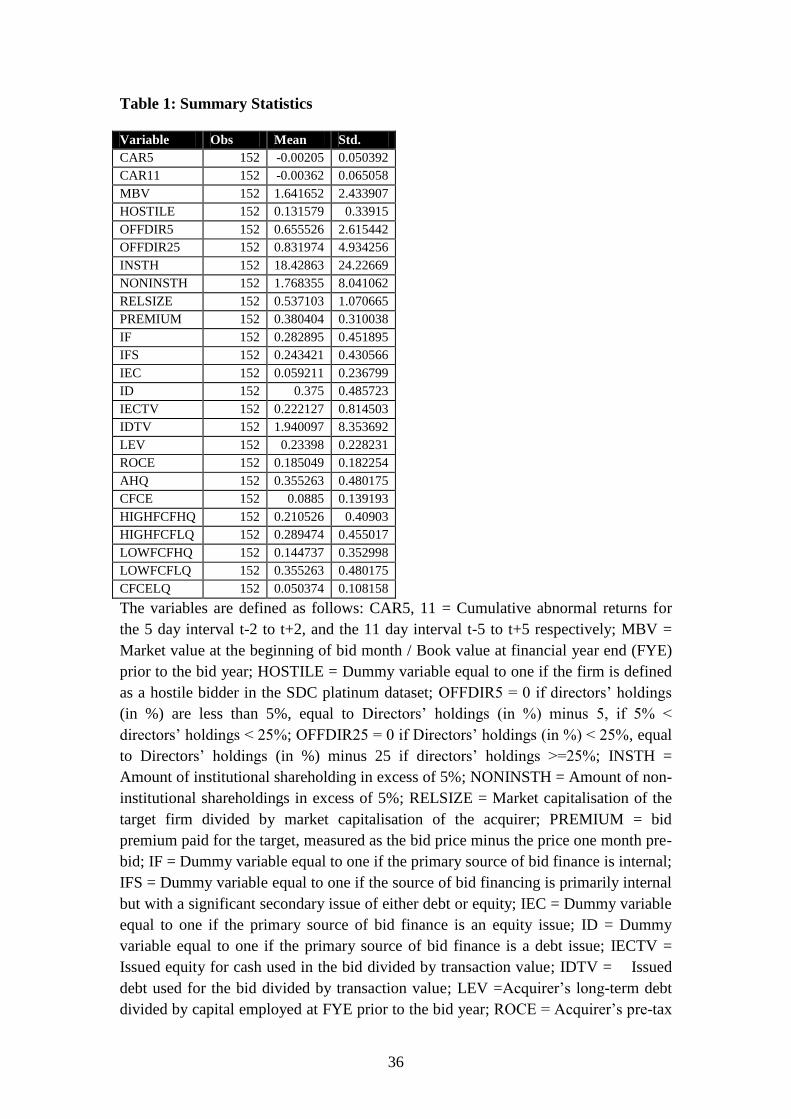
Definition of Variables

AHQ = Dummy variable equal to one if the acquiring firm has low BMV (high q

ratio) relative to its industry BMV

CAR5, 11 = Cumulative abnormal returns for the 5 day interval t-2 to t+2, and the 11

day interval t-5 to t+5 respectively

CFCE = FCF one year prior to the bid year divided by capital employed

CFCELQ = CFCE if the firm‟s AHQ is equal to zero, zero otherwise

HFCHQ = Dummy variable equal to one if the firm has high CFCE (greater than the

sample median) and AHQ equal to one

HFCLQ =Dummy variable equal to one if the firm has high CFCE (greater than the

sample median) and AHQ equal to zero

HOSTILE = Dummy variable equal to one if the firm is defined as a hostile bidder in

the SDC platinum dataset (cross-checked with Acquisitions Monthly)

ID = Dummy variable equal to one if the primary source of bid finance is a debt issue

IDTV = Issued debt used for the bid divided by transaction value

IEC = Dummy variable equal to one if the primary source of bid finance is an equity

issue

IECTV = Issued equity for cash used in the bid divided by transaction value

IF = Dummy variable equal to one if the primary source of bid finance is internal

IFS = Dummy variable equal to one if the source of bid financing is primarily internal

but with a significant secondary issue of either debt or equity.

INSTH = Amount of institutional shareholding in excess of 5%12

LEV =Acquirer‟s long-term debt divided by capital employed at FYE prior to the bid

year

LFCHQ =Dummy variable equal to one if the firm has low CFCE (less than the

sample median) and AHQ equal to one

LFCLQ = Dummy variable equal to one if the firm has low CFCE (less than the

sample median) and AHQ equal to zero

MBV = Market value at the beginning of bid month / Book value at financial year end

(FYE) prior to the bid year

NONINSTH = Amount of non-institutional shareholdings in excess of 5%

12

See footnote 8.

19

OFFDIR5 = 0 if directors‟ holdings (in %) are less than 5%13

, or equal to Directors‟

holdings (in %) minus 5, if 5% < directors‟ holdings < 25%

OFFDIR25 = 0 if Directors‟ holdings (in %) < 25%, or equal to Directors‟ holdings

(in %) minus 25 if directors‟ holdings >=25%

PREMIUM = bid premium paid for the target, measured as the bid price minus the

price one month pre-bid

RELSIZE = Market capitalisation of the target firm divided by market capitalisation

of the acquirer

ROCE = Acquirer‟s pre-tax profit before the bid divided by capital employed

In calculating short run returns, we use a simple market adjusted returns model using

the FT All Share Index (FTASI) as our market proxy, to calculate cumulative

abnormal returns over the intervals day t-20 to day t+20, day t-5 to day t+5, and day

t-2 to day t+2. Draper and Paudyal (2008) also employ a market adjusted returns

model. We favour a simple market adjusted returns measure as it avoids any thin

trading problems inherent in using daily returns to calculate market-model

parameters. The significance of abnormal returns can be estimated as in Brown and

Warner (1985), but as a robustness check we also calculate the bootstrapped

skewness-adjusted t-statistic, more normally associated with the testing of long run

abnormal returns, from Lyon et al (1999). However, whilst expanding the window

from 5 days around announcement to 11 days seems to capture a significant increase

in market reaction, expanding the window to 41 days around announcement merely

adds noise. As such, we drop the 41 day CARs and concentrate our regression tests

on the 11-day window. A summary of these variables, together with their means and

standard deviations, is given in Table 1.

It is well-documented that longer term returns to acquisitions are as a whole are

significantly less than zero, although the evidence on returns to cash acquisitions is

mixed (see, for example, Agrawal and Jaffe, 2000). In the UK, Gregory (1997) shows

that long run abnormal returns to cash acquirers are negative, but not significantly so.

More recently, Conn et al (2005) show that domestic cash acquirer performance over

13

Note: For the earlier years in our sample, companies were only required to notify the Stock Exchange

of holdings in excess of 5% of total shareholdings, so that holdings of less than 5% are simply

unobservable. This threshold was later reduced to 3%, but for consistency we retain the 5% limit.

20

the period 1984-1998 is virtually zero. A question investigated in this paper is

whether that long run performance might vary according to the source of cash, and

whether it varies with FCF. A consensus seems to be emerging that whilst buy and

hold abnormal returns (BHARs) are useful for depicting the experience of investors,

statistical inference from BHARs is highly problematic.14

The properties of calendar

time abnormal returns (CTARs) avoids the problem of cross sectional dependence in

the abnormal returns (Mitchell and Stafford, 2000), although as Loughran and Ritter

(2000) point out, CTAR tests will be weak if managers exercise “behavioural timing”

in corporate financing decisions. Given this emerging consensus, we base our

analysis of long run abnormal returns on CTARs. The question then arises of how

best to estimate these CTARs. Whenever we calculate abnormal returns in calendar

time, we have the choice between measuring returns relative to a risk-controlled

benchmark, or using a regression-based framework, such as the Fama-French model.

Lyon et al. (1999, p.197) suggest that simple CTAR methods appear to be better

specified (and more conservative) than the Fama-French three factor approach.

Mitchell and Stafford (2000, p.321) also favour the control-portfolio CTAR

methodology rather than the Fama-French regression-based approach, noting that

because it suffers from fewer statistical flaws “more faith should be placed in these

results”. However, against this Ang and Zhang (2004) provide evidence in favour of

the Fama-French model, but specifically advise against using the Carhart four factor

model in tests. Their simulation results suggest that in calendar time, the Fama-

French method is well-specified, but they also show that more powerful tests result

from using weighted least squares (WLS) rather than ordinary least squares (OLS).

An added concern for UK researchers is that it is far from clear that the Fama-French

model is entirely appropriate in a UK context (Gregory, Harris and Michou, 2001; Al-

Horani, Pope and Stark, 2003; Michou, Mouselli and Stark, 2007; Gregory, Tharyan

and Huang, 2009). These contradictory findings in the literature lead us to adopt two

approaches to the estimation of CTARs: a control firm approach, which follows that

used in a recent study of UK IPOs (Gregory, Guermat and Al-Shawawreh, 2010); and

a WLS Fama-French model following Ang and Zhang (2004).

14

See, for example, Brad Barber‟s recent seminar at the Financial Management Association

Conference, Reno, October 2009.

21

The Gregory et al (2010) model allows for some variation between the characteristics

of the benchmark portfolio and the characteristics of the event firm portfolio, and also

deals with the problem of heteroscedasticity. To implement this we regress the

portfolio of cash acquirers on a size-matched control portfolio. Let tR , be the time

series of a portfolio of the returns of acquiring companies that undertake a cash

takeover within the previous τ months. We undertake the basic calendar time test by

testing for the significance of in a time series model

t

E

tt RR )( ,, (1)

where E

tR )( , is the required (or benchmark) return and t is a zero mean disturbance

term.

The innovation in their paper is to allow for heteroscedasticity in the CTARs by using

a GLS approach. For an equally weighted portfolio, the -month calendar time

portfolio return is:

, ( )

, 1,

1 tn

t itit

R Rn

(2)

where tn , is the number of firms in the portfolio and )(itR is the return of a firm i

that was a cash acquirer within the last months. The assumption is that the

variance of this calendar time portfolio can be approximated by some function of

tn10ˆˆ , and to ensure that the variance is positive they assume

)ˆˆexp()(ˆ10 ttt nuraV . They then operationalise the model by taking the

unrestricted residuals tu from

tbtt uRR ,

And then by estimating the regression

ttt errornu )log()ˆlog( 10

2

Finally, they estimate ))log(ˆˆexp()(ˆ10 tt nuraV . As Gregory et al (2010) show,

this GLS formulation offers a better fit in terms of adjusted R-squared statistics than

the alternative White (1980) heteroscedasticity-corrected standard errors. We find a

22

similar result in this paper, although inferences from the White (1980) approach are

broadly similar. Note that conceptually, this model can be applied perfectly well to

the Fama-French model, and indeed we do so. Nonetheless, given the evidence in

Ang and Zhang (2004) relates solely to WLS, we only report these WLS results in the

paper. However, results are slightly stronger from the GLS method. Inferences are

generally the same, with the exception of one of our portfolios which we identify

below.

Specifically, the Fama-French three factor model regression which we estimate is:

tttftmtftt HMLhSMBsRRbaRR .., (3)

The Fama-French factors are described in Gregory, Tharyan and Huang (2009) and

downloaded from their website. The factors are constructed so as to mimic, as closely

as possible, the US factors available on Ken French‟s data pages.

Finally on the subject of long term returns, whilst CTARs have the inference

advantages referred to above, one disadvantage is that they do not lend themselves to

the regression-based tests we use for CARs. So instead, we partition our sample

according to form of financing, and by FCF and q.

Results

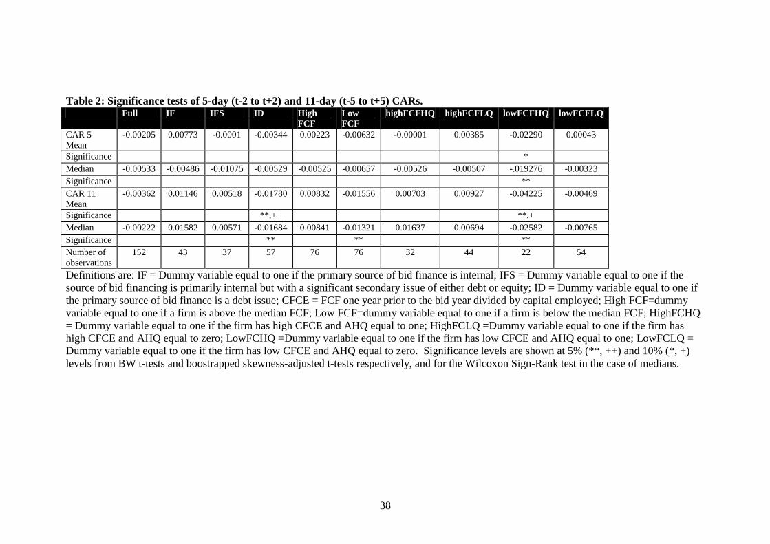
Our first results are those based upon CARs partitioned by form of financing, FCF

and q and FCF, in Table 2. Overall, the 5-day CARs are an insignificant -0.2%,

whilst the 11 day CARs are -0.36%, though still insignificant. The only financing

sub-group to record a significant 11-day return is the debt issuing group.15

Here, the

CAR is -1.78%, significant at the 5% level using both a Brown-Warner t-test or the

bootstrapped skewness-adjusted t-test. For both windows, the internal financing

group show the best returns, although these returns are not significant at conventional

levels. As a further check that these results are not being driven by outliers, we also

report medians and test the significance of the medians using a Wilcoxon Sign-Rank

test. Medians are close to the means, and again the 11-day CAR for the ID group is

15

Note that throughout the partitioned tests, we do not report CARs or CTARs for the mixed and

equity-issuing categories as the number of firms is too small to allow meaningful inferences to be

drawn. We do, however, include dummy variables for these categories in the regression tests.

23

significantly negative at the 5% level. Although modest, these preliminary results

provide more support for the pecking-order hypothesis than the FCF hypothesis.

Partitioning by FCF shows that both short window and longer window CARs are

positive for high FCF firms, and negative for low FCF firms, though none of the

figures are significant except in the case of the -1.3% median for the low FCF group.

However, when we partition on the basis of both q and FCF, we see that the worst

returns are for low FCF, high q firms, which record a return of -2.3% over 5 days, and

-4.2% over 11 days. The former is significant at the 10% level using a the BW t-test,

whereas the latter is significant at the 5% level using both BW and bootstrapped

skewness-adjusted t-tests. Although medians are closer to zero than the means, they

are significantly negative for this group at the 5% level for both 5 day and 11 day

windows.

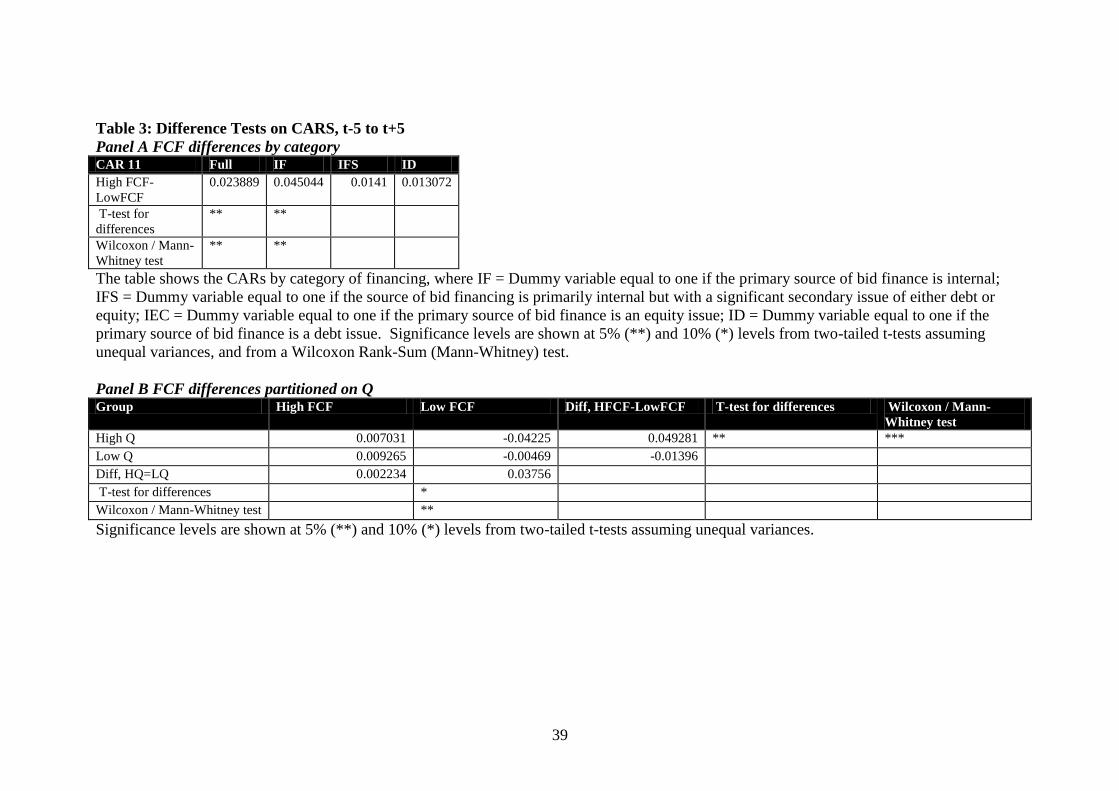
Table 3 then partitions the 11-day CARs by both FCF difference and cash-source

category (Panel A) and by FCF and q (Panel B). Differences are tested using a two-

tailed t-test assuming unequal variances, and by a non-parametric Wilcoxon Rank-

Sum (or Mann-Whitney) test. Overall, the high FCF firms have CARs that are 2.4%

higher than their low FCF counterparts, the difference being significant at the 5%

level for both the t-test and non-parametric tests. When we partition by the source of

funds we find that the largest, and significant, difference in CARs is in the internal

financing category. Here, the high FCF firms have returns that are 4.5% higher than

low FCF firms, and again this result is also significant at the 5% level using a non-

parametric test. In every source of financing sub-sample, high FCF firms have better

returns than low FCF firms, although the differences are not significant in the case of

the IFS and ID firms. Panel B shows the results when firms are partitioned by q and

FCF. Recall that the FCF hypothesis predicts that high FCF, low q firms are the

problem case. As we have already seen from Table 2, the bad news for the FCF

hypothesis is that this category of firms turns out to have the best overall

performance. However, the 1.4% difference in CARs between high and low FCF

firms in the low q category fails to be significant. Ironically, it is FCF differences

amongst high q firms that turn out to be significant, with high FCF firms out-

performing low FCF firms by 4.9%. This result is significant at the 5% level using a

t-test, and at the 1% level when we employ the non-parametric test. Amongst high

FCF firms, q differences are insignificant in explaining returns, but in the low FCF

24

group high q firms under-perform low q firms by 3.8%, significant at the 10% level

under a t-test, but significant at the 5% level using a non-parametric test. All our

results so far are robust to using our alternative cash stock ratio measure, where high

cash stock firms are defined as those with a cash stock ratio greater than unity.

On the basis of the results so far, there is little support for the FCF hypothesis.

Announcement returns are the opposite to those predicted by the hypothesis, with

high FCF firms out-performing low FCF firms, and, most tellingly, low FCF high q

firms experiencing significant negative returns. In addition, firms that acquired for

cash principally funded by an increase in debt seem to experience worst returns than

those choosing internal finance. We now turn to more rigorous tests of the hypothesis

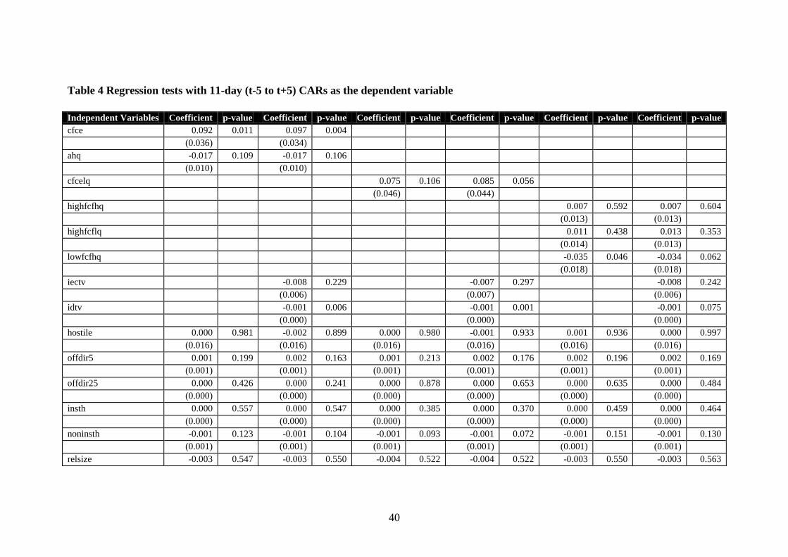
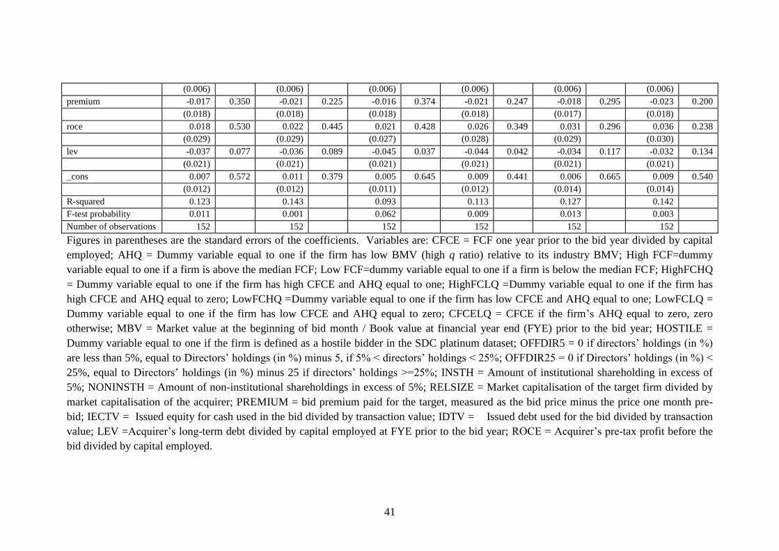
that control for our firm-specific variables. In Table 4, we run regressions with the 11

day CAR as the dependent variable, and with all control variables included. All t-

statistics are calculated using White (1980) corrected standard errors. The basic

models we use to test the FCF hypothesis are as follows. Model 1A includes both the

CFCE, the free cash flow proxy, and AHQ, the proxy for high q bidders. Model 1B

adds the actual financing proportions IECTV and IDTV to the FCF measures and the

control variables. Models 2A and 2B repeat the experiment, but using CFCELQ as

the free cash flow proxy. Model 3 then reports results (including financing

proportions) using HighFCFHQ, HighFCFLQ (the category predicted to experience

negative market returns under the FCF hypothesis) and LowFCFHQ dummies, with

lowFCFLQ forming the base case (and hence being picked up by the constant).

In Columns 1 and 2 of Table 4 (Model 1A) we see that none of the control variables

are significant at conventional levels, that AHQ has a negative but not quite

significant (p=0.109) impact on announcement period returns, but that CFCE has a

significant positive impact. Pre-bid leverage has a weakly significant negative

association with returns. These result holds for Model 1B (columns 3-4) and further

suggests that the proportion of issued debt has a negative impact on performance, the

effect is not significant. For Model 2A, we have the result that CFCELQ just fails to

have a significant positive impact (Cols 5-6), but once we include the financing

proportion variables the coefficient is significantly positive (p=0.056). Once again,

pre-bid leverage has a negative association with returns (p=0.037 and 0.042 for

models 2A and 2B respectively) and the proportion of debt issued is a highly

25

significant predictor of negative announcement period returns. Finally, Models 3A

and 3B in the final four columns of Table 4 show that significant negative returns of -

3.5% or -3.4% (Models 3A and 3B respectively) come from the lowFCF, high q sub-

group. The FCF-hypothesised “problem” group, highFCF, low q, have positive, but

insignificant, returns equivalent to 1.1% and 1.3% respectively. However, in the case

of Models 3A and 3B pre-bid leverage loses its significant explanatory power. These

results are similar when the cash stock ratio is employed as our measure of FCF,

except that the equivalent of the CFLQ measure simply fails to be significant at

conventional levels.

There is no hint in any of our results that high free cash flow is negatively associated

with bidder performance, nor that using high levels of debt to finance a bid is

perceived as beneficial by the market. Rather, it seems as though having low levels of

free cash flow is regarded as a negative signal by markets, and that this is particularly

true in the case of high q firms. To the extent that it is significant, the use of

extensive debt financing appears to have a negative association with announcement

period returns, and high levels of pre-bid leverage are also, to some extent, associated

with negative performance in cash bids. Furthermore, once FCF is controlled for it

appears that firms which use internal financing do better than firms that use other

sources of funding for their cash bids. Taken as a whole, these announcement period

results contradict the FCF hypothesis, and are more consistent with markets viewing

acquirers that have high FCF levels as having lower financial distress risk. As a final

robustness check, we re-ran the regressions including market timing variables known

either to predict the market risk premium or future returns (Harris and Sanchez-Valle,

2000), or to influence the choice of financing method. These variables were: the prior

12 months return on the market; the dividend yield on the market; the Treasury Bill

rate; and the difference between the long gilt rate and the Treasury Bill rate. As none

of these variables turned out to be significant in predicting the CARs, nor did they

change our inferences, we do not report those regressions here.16

As we note above, in general UK company law and the City Code places greater

emphasis on shareholder rights relative to manager rights than does US law. We

16

The authors are grateful to Paul Draper for suggesting this robustness check.

26

further argued that strong institutional shareholding in the UK was likely to reinforce

that position. One obvious test is to examine whether high FCF is less of a problem in

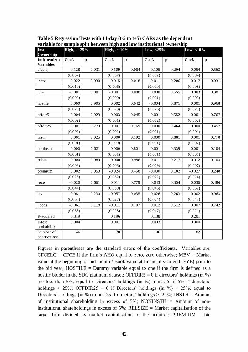
high institutional ownership firms than low institutional ownership firms. We split

our sample using the 25% threshold explained above, and run separate parsimonious

regressions on our CFCELQ variable for high and low ownership firms.17

As a

further robustness check, we change the institutional ownership threshold to 10%.

The results are reported in Table 5. The first two columns show the results from the

high institutional ownership group (n = 46), and confirm that in this sub-group, high

FCF firms have positive returns, but high gearing firms have negative returns. IDTV

is negative, and highly significant and intriguingly IECTV is significantly positive.

Last, within this group returns seem to be positively related to institutional ownership

and modest levels of directors‟ ownership. However, in the low institutional

ownership sub-group in columns 5 and 6 (n=106), explanatory power is far lower, and

although CFCELQ and LEV retain the same signs, neither is significant. We re-run

the regressions using a more modest cut-off for institutional ownership of 10%. The

results are reported in Columns 3-4 of Table 5 for the high ownership group, and the

final columns of Table 5 for the low ownership group. The central results on

CFCELQ and IEDTV are unaltered, as is IECTV, but note that LEV now becomes

significantly negative. For the low ownership group, only IECTV is a significant

negative predictor of abnormal returns. It seems that even modest levels of

institutional ownership are enough to ensure high FCF and low gearing are positive

indicators of the likely success of the acquisition. We see this as consistent with our

argument that good monitoring, coupled with high levels of shareholder rights, is able

to overcome any agency conflicts affecting the financing of any cash acquisition.

However, these effects are not robust to the use of a cash stock ratio, as when we

substitute our cash stock ratio measure for CFCELQ the variable is simply

insignificant.

Of course, given the findings from the long-term acquirer performance literature, it

may be that at announcement markets under-react to news about the takeover. It

could be the case that markets simply fail to anticipate the full importance of free cash

flow at the time of the takeover. Furthermore, it can be argued that by looking at the

17

We run separate regressions as factors affecting performance in both groups turn out to be very

different.

27

change in consolidated debt and acquirer equity over the year of takeover, our

methods of determining bid financing necessarily involve some look ahead bias. A

comprehensive test of the hypothesis therefore requires us to examine long run

returns. As in the case of many long term studies (Agrawal, Jaffe and Mandelker,

1992; Loughran and Vijh, 1997; Rau and Vermaelen, 1998), we choose to look at

returns for the 60-month period following the acquisition. Note, however, that Ang

and Zhang (2004) show that whilst long-horizon CTAR returns from the three-factor

model are well specified, they have low power to detect abnormal returns at long

horizons. Table XI in Lyon et al (1999) also suggests that tests using control

portfolios are generally well specified, but tend to be more conservative than

inferences from the Fama-French regressions at the 60 month horizon, particularly

with regard to the detection of negative abnormal performance.18

Ang and Zhang

(2004, p.266-7) also note that the FF regressions have lower power to detect negative

induced returns, particularly at long horizons.

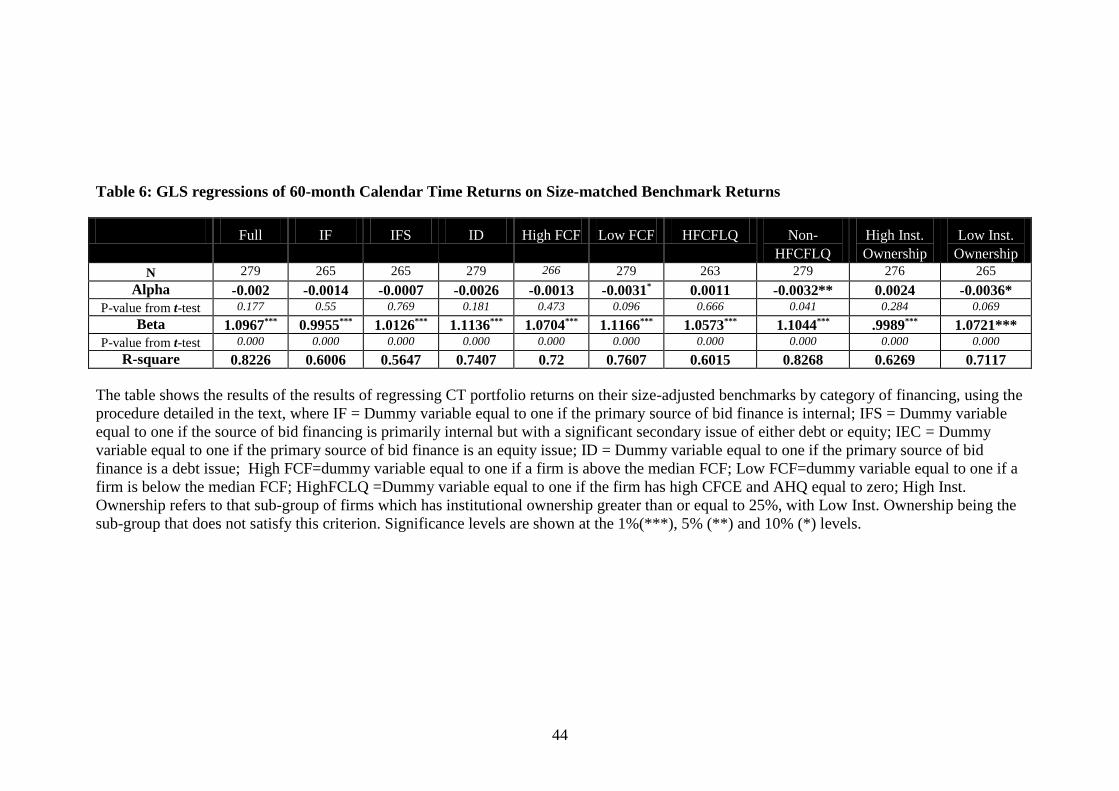
Turning to the results themselves, Table 6 presents the results for the GLS model of

Gregory et al (2010). Overall, and in line with previous findings on UK cash

takeovers, alphas are slightly negative but not significantly different from zero.

Looking at the different financing groups, we see that although the debt issuers have

the worst performance, at -0.26% per month, the effect is not significant. However,

when we turn to the results partitioned on FCF, we see that low FCF firms register a

significant (at the 10% level) negative abnormal return of -0.31% per month. One

difficulty with partitioning too finely on a small sample is that the sub-grouping tend

to be too small to exhibit significance. This is a particular problem when partitioning

on both q and FCF, and we deal with this by simply partitioning into the hypothised

“problem” group of High FCF, Low q firms and compare them to remaining firms.

When we do so, it turns out that the high FCF, low q sub-group of acquirers that are

hypothesised to have the worst performance under the FCF hypothesis actually

exhibit insignificant positive performance, whereas the remainder exhibit significant

negative performance of -0.32% per month.

18

Specifically, the rejection rate in random samples is 1.3% compared to a theoretical level of 2.5%.

28

Given our announcement period results, we also partition on the basis of institutional

ownership. In the final two columns of Table 6 we report the high (>=25%)

institutional and low (< 25%) institutional ownership sub-samples. The former have

an insignificant positive return, but the latter exhibit a significant (at the 10% level)

negative return of -0.36% per month.

In Table 7, we present the results from the Ang and Zhang (2004) preferred Fama-

French WLS regressions. These produce similar, but somewhat stronger, results than

those from Table 6. Again, debt issuers are the worst performing sub-group with a

negative return of -0.28% per month, although the significance level is only 15.2%.

The high FCF group exhibit a performance that is very close to zero. By contrast, the

low FCF group have significant returns of -0.37% per month. In addition, we see that

the low FCF group carry higher risk factor loadings on each of the three Fama-French

factors than the high FCF group. This is consistent with low FCF acquirers having a

greater degree of distress risk. Once again, the high FCF, low q group have

insignificant positive returns but the remainder (non High FCF, low q firms) have

returns that are a highly significant -0.36% per month. This group also carries the

highest exposure to market risk and the HML factor. Finally, the results for the

institutional ownership partition confirm those in Table 6. It is the low ownership

sub-group that have the worst (and significant) negative performance, and they also

have a higher exposure to market and HML risk (though a lower small company risk).

Conclusions

In this paper, we have argued that a clean test of the FCF hypothesis can be conducted

by focussing on pure cash takeovers. Indeed, Jensen himself sets up the motivation

for this study when (1988, p. 34) he makes a the following claim: „free cash flow

theory implies that managers of firms with unused borrowing power and large free

cash flows are more likely to undertake low-benefit or even value destroying

mergers‟. We argue that looking at pure cash takeovers goes to the heart of this claim.

Following Gompers et al (2003), and Cremers and Nair (2005), we hypothesised that

the combination of strong shareholder rights and significant monitoring from

institutional shareholders may significantly reduce any agency problems caused by

high FCF. As the UK is characterised by an environment that has low protection

against takeovers, and high levels of institutional shareholding, it offers an excellent

29

testing ground for this hypothesis. When we test the FCF hypothesis in the UK

environment, our results provide no evidence to support the FCF hypothesis. Both

announcement period and long terms returns show that acquirers with low free cash

flow, not high free cash flow, are associated with acquisitions that damage

shareholder wealth. Indeed, the sub-grouping of firms with high FCF and low q ratios

is the only grouping to exhibit positive (although not significant) long-run returns.

Analysis of announcement period returns further suggest that high levels of pre-bid

leverage may also have a negative impact on shareholder wealth. In addition, we

provide evidence from announcement period returns that relying on internal finance to

finance cash acquisitions may be beneficial, whilst a reliance on debt financing may

be detrimental. However, whilst these effects carry through to the longer term, they

are not statistically significant at long horizons. Finally, we show that the benefits of

having a high FCF seem to be greatest in firms financing acquisitions from internal

finance.

A question that we explore is why the UK evidence is so different from that of the

US. Of course, using the standard La Porta et al (1998) scoring of governance, the

US and the UK do not look that different. However, consistent with Cremers and

Nair (2005), we argue that it is the stronger position of shareholders relative to firm

managers that is important in the UK (Bush, 2005; Sudarsanam, 2000), and that

furthermore the high level of institutional ownership coupled with a high

concentration of fund managers (Stapledon and Bates, 2002) plays an important role

in monitoring. Consistent with that, we show that the positive effects of high FCF

and the negative effects of high leverage are concentrated in high institutional

ownership firms, although the former effect is not observed when we run our

regressions using a cash holding, rather than a cash flow, proxy for FCF. One

explanation is that strong shareholder rights and good monitoring are capable of

overcoming any inherent agency problems associated with high levels of FCF.

However, we acknowledge that an alternative explanation is simply that the more

liberal market for takeovers in the UK serves to discipline managers, an effect that

would be predicted by the FCF hypothesis.

In addition, our findings may be viewed as providing some support for the Myers and

Majluf (1984) pecking-order theory. Our results also provide support for a theory

30

where low FCF and high leverage predict financial distress. Our regression tests

show that this result is not simply an artefact of firm profitability, in that high FCF is

positively associated with bidder returns even after ROCE is controlled for.

Unfashionable as it may have been (at least until recently), we show that far from

being undesirable, having higher levels of free cash flow and lower levels of debt can

be associated with the superior performance of cash acquirers, provided strong

shareholder rights and institutional shareholder monitoring is present.

Acknowledgements: The authors are grateful to: George Bulkley (University of

Bristol); Matt Cain (Notre Dame University); Paul Draper (University of Leeds);

David Gwilliam (University of Exeter); Luc Renneboog (Tilburg University); Ian

Tonks (University of Bath); and session participants at the New York Financial

Management Association Conference, October 2010 for their helpful comments on

earlier drafts of this paper. The usual caveats on errors and omissions apply.

REFERENCES

Agarwal, V. and Taffler, R.J. (2007), „Twenty-five years of the Taffler z-score model:

does it really have predictive ability?‟, Accounting and Business Research, Vol 27 (4)

pp285-300.

Agarwal, V. and Taffler, R. (2008). „Does Financial Distress Risk Drive the

Momentum Anomaly?‟ Financial Management (Autumn), pp 461 - 484

Agrawal, A., and Jaffe, F.E. (2000), „The post merger performance puzzle‟, in

Advances in Mergers and Acquisitions, Cooper, C. and Gregory, A. (eds), JAI Press,

New York pp.7-41.

Agrawal, A., Jaffe, J.F. and Mandelker, G.N. (1992), 'The post-merger performance

of acquiring firms; a re-examination of an anomaly', Journal of Finance, Vol. 47,

No.4, pp 1605-22

Al-Horani, A., Pope, P.F. and Stark, A.W. (2003). „Research and Development

Activity and Expected Returns in the United Kingdom‟, European Finance Review

Vol. 7, No. 1, pp 27-46.

Ang, J.S. and Cheng, Y. (2006) „Direct evidence on the market-driven acquisition

theory‟, Journal of Financial Research, Vol. 29, pp. 199-216

Ang, J.S. and S. Zhang (2004) „An Evaluation of Testing Procedures for Long

Horizon Event Studies‟, Review of Quantitative Finance and Accounting, Vol. 23, pp

251-274.

Baker, M. and J. Wurgler, (2002), „Market Timing and Capital Structure‟, The

Journal of Finance, Vol. 57, No. 1, pp1-32

31

Bi, X. G. and A. Gregory (2009), „Stock Market Driven Acquisitions versus the Q

Theory of Takeovers - The UK Evidence‟, Working Paper, The University of Exeter,

Xfi, http://papers.ssrn.com/sol3/papers.cfm?abstract_id=1291693

Brown S. J., and J. B. Warner (1985), „Using Daily Stock Returns: The Case of Event

Studies‟, Journal of Financial Economics, Vol. 14, pp. 3-31

Bush, T. (2005). Divided by common language. Where economics meets the law: US

versus non-US financial reporting models. Institute of Chartered Accountants in

England and Wales, London, . June 2005.

Campbell J. Y., Hilscher, J. and Szilagyi, J. (2008), „In Search of Distress Risk‟,

Journal of Finance, Vol. 63, No. 6, pp 2899-2939

Christidis, A. C.Y. and Gregory, A (2010), „Some New Models for Financial Distress

Prediction in the UK‟, Xfi Centre Working Paper, University of Exeter.

Conn, R.L, Cosh, A. Guest, P. and Hughes, H. (2005), „The impact on UK acquirers

of domestic, cross-border, public and private acquisitions‟, Journal of Business

Finance and Accounting, Vol.32 (5)&(6), pp.815-70.

Cremers, K.J.M And V. B. Nair (2005). „Governance Mechanisms and Equity Prices‟.

The Journal of Finance, Vol. 60, No. 6, pp. 2859-2894

Dimson, E., Marsh, P. and Staunton, K. (2005), Global Investment Returns Yearbook,

2005, London: ABN AMRO/ LBS.

Dong, M., Hirshleifer, D., Richardson, S., and Teoh, S.H. (2006) „Does investor

misevaluation drive the takeover market?‟, The Journal of Finance, Vol. 61, No. 2, pp.

725-762

Doukas, J. (1995) „Overinvestment, Tobin‟s Q and Gains from Foreign Acquisitions‟,

Journal of Banking and Finance, Vol. 19, pp1285-1303

Draper, P. and Paudyal, K. (2006), „Acquisitions: Private versus Public‟, European

Financial Management, Vol. 12, No. 1, pp. 57–80

Draper, P. and Paudyal, K., (2008) „Information Asymmetry and Bidders‟ Gains‟,

Journal of Business Finance and Accounting, Vol.35 (3)&(4), pp.376-405

Fama, E.F. and French, K.R. (1997), „Industry costs of equity‟, Journal of Financial

Economics, 43, pp 153-193.

Franks, J. R., Harris, R. S. and C. Mayer (1988), „Means of Payment in Takeovers:

Results for the United Kingdom and the United States‟, in Corporate Takeovers:

Causes and Consequences edited by Alan J. Auerbach, pp. 221-264

32

Goergen, M. and L. Renneboog (2004), „Shareholder Wealth Effects of European

Domestic and Cross-border Takeover Bids‟, European Financial Management, Vol.

10, No. 1, pp. 9-45

Gompers, Paul A., Joy L. Ishi, and Andrew Metrick, (2003), „Corporate governance

and equity prices‟, The Quarterly Journal of Economics, Vol. 118, No. 1, pp. 107-155

Greene, W.H. (2000), Econometric Analysis, 4th

ed., Upper Saddle River, NJ: Prentice

Hall.

Gregory, A. (1997), „An Examination of the Long Run Performance of UK Acquiring

Firms‟, Journal of Business Finance and Accounting, Vol.24 (7)&(8), pp. 971-1002.

Gregory, A. (2000). „Motives underlying the method of payment by UK acquirers: the

influence of goodwill‟, Accounting & Business Research, Vol. 30, No. 3, pp. 227-240

Gregory, A. (2005), „The Long Run Abnormal Performance of UK Acquirers and the

Free Cash Flow Hypothesis‟, Journal of Business Finance & Accounting, Vol.32

(5)&(6), pp. 777-814

Gregory, A. , C.Guermat and F. Al-Shawawreh (2010) „UK IPOs: Long Run Returns,

Behavioural Timing and Pseudo Timing‟ Journal of Business Finance and

Accounting, forthcoming.

Gregory, A., Harris, R.D.F. and Michou, M. (2003). „Contrarian Investment and

Macroeconomic Risk‟ Journal of Business Finance & Accounting, Vol. 30(1)&(2), pp

213-255.

Gregory, A. and Matako, J. (2005). „Long run abnormal returns to acquiring firms: the

form of payment hypothesis, bidder hostility and timing behavior‟, Xfi Centre,

University of Exeter Working Paper, http://xfi.exeter.ac.uk/workingpapers/0502.pdf

Gregory, A., and Michou, M. (2009). „Industry Cost of Capital: UK Evidence‟,

Journal of Business Finance and Accounting, June/July, pp 679–704.

Gregory, A., Tharyan, R. and Huang, A. (2009) „The Fama-French and Momentum

Portfolios and Factors in the UK‟

http://papers.ssrn.com/sol3/papers.cfm?abstract_id=1506960

Hall, B. (1998). Innovation and Market Value. Paper presented to NIESR conference

on Productivity and Competitiveness, London, 1998.

Hansen, R.G. (1987), „A Theory for the Choice of Exchange Medium in Mergers and

Acquisitions‟, Journal of Business, Vol. 60, No. 1 pp. 75-95

Harford, J. (1999) „Corporate Cash Reserves and Acquisitions‟. Journal of Finance

54(6) 1969-97.

Harris, M. and A. Raviv (1990), „The Capital Structure and the Information Role of

Debt‟, Journal of Finance, Vol. 45, No. 2, pp. 321-349

33

Harris, R.D.F. and R. Sanchez-Valle (2000), „The Gilt-Equity Yield Ratio and the

Predictability of UK and US Equity Returns‟, Journal of Business Finance and

Accounting, 27 (3&4), April/May, pp. 333-357.

Jensen, M.C. (1986) „Agency Costs of Free Cash Flow, Corporate Finance, and

Takeovers‟, American Economic Review, Vol.76, No. 2, pp.323-329.

Jensen, M.C. (1988) „Takeovers: Their Causes and Consequences‟, Journal of

Economic Perspectives, Vol. 2, No. 1, pp.21-48.

Jensen, M.C. (1991), „Corporate Control and the Politics of Finance‟, Journal of

Applied Corporate Finance, Vol. 4, No. 2, pp. 13-34

La Porta, R., Lopez-de-Silanes, F., Shleifer, A., Vishny, R., (1997). „Legal

determinants of external finance.‟ Journal of Finance, Vol. 52, No 3, pp. 1131–1150.

La Porta, R., Lopez-de-Silanes, F., Shleifer, A., Vishny, R., (1998). „Law and

finance‟. Journal of Political Economy, Vol. 106, No. 5, pp. 1113–1155.

Lang, L.F.P., Stulz, R.M. and R.A. Walkling (1991), „A Test of the Free Cash Flow

Hypothesis: The Case of Bidder Returns‟, Journal of Financial Economics, Vol. 29,

No. 2, pp. 315-355

Loughran, T. and J.R. Ritter (1995) “The new issues puzzle”, Journal of Finance, Vol.

50, No. 3, pp. 23-51.

Loughran, T. and J. R. Ritter (2000) “Uniformly least powerful tests of market

efficiency”, Journal of Financial Economics, Vol. 55, No.3, pp. 361-389

Loughran, T. and A. M Vijh,. (1997), „Do Long-Term Shareholders Benefit From

Corporate Acquisitions?‟, Journal of Finance, Vol 52, No. 5, pp. 1765-1790.

Lyon, J.D., Barber, B.M. and C-L. Tsai (1999), „Improved Methods for Tests of

Long-run Abnormal Stock Returns‟, Journal of Finance, Vol. 54, No. 1, pp. 165-201

Martynova, M. and L. Renneboog (2009), „What determines the financing decision in

corporate takeovers: Cost of capital, agency problems, or the means of payment?‟,

Journal of Corporate Finance, Vol. 15, No. 3, pp 290-315.

Martynova, M., Renneboog, L., (2008). „Spillover of corporate governance standards

in cross-border mergers and acquisitions.’ Journal of Corporate Finance Vol. 14, No.

3, pp. 200–223

Martin, K. J. (1996), „ The Method of Payment in Corporate Acquisitions, Investment

Opportunities, and Management Ownership‟, Journal of Finance, Vol. 51, No. 5, pp.

1227-1246.

34

Michou, M., Mouselli, S. and Stark A.W. (2007). „Estimating the Fama and French

Factors in the UK: An Empirical Review‟, Manchester Business School Working

paper series, http://www.mbs.ac.uk/research/workingpapers/index.aspx?AuthorId=381

Mitchell M. L. and E. Stafford (2000), „Managerial Decisions and Long-Term Stock

Price Performance‟, The Journal of Business, Vol. 73, No. 3, pp. 287-329

Myers, S.C. (1984), „The Capital Structure Puzzle‟, The Journal of Finance, Vol. 39,

No. 3, pp. 575-592

Myers, S.C. and N. Majluf, (1984), „Corporate Financing Decisions When Firms

Have Investment Information that Investors Do Not‟, Journal of Financial Economics

Vol. 13, No. 2, pp. 187-221

Rau, P.R. and T. Vermaelen, (1998), „Glamour, value and the post-acquisition

performance of acquiring firms‟, Journal of Financial Economics, Vol. 49, No. 2, pp.

223-253

Roll, R. (1986), „The Hubris Hypothesis of Corporate Takeovers‟, Journal of

Business, Vol. 59, No. 2, pp 197-216

Savor, P.G, and Lu, Q. (2009), „Do Stock Mergers Create Value for Acquirers?‟

Journal of Finance, Vol. 64, No. 3, pp 1061-1097.

Shleifer, A. and Vishny, R.W (2003), „Stock market driven acquisitions‟, Journal of

Financial Economics Vol. 70, No. 3, pp. 295-311

Stapledon, G. P. and Bates, J. J. (2002), "Reducing the Costs of Proxy Voting" in J.

McCahery, P. Moerland, T. Raaijmakers and L. Renneboog (eds), Corporate

Governance Regimes: Convergence and Diversity, Oxford University Press, Oxford:

pp 567-602.

Stulz, R.M. (1990), „Managerial Discretion and Optimal Financing Policies‟, Journal

of Financial Economics Vol. 26, No. 1, pp. 3-27

Sudarsanam, S. (2000) „Corporate Governance, Corporate Control and Takeovers‟, in

Advances in Mergers and Acquisitions, Cooper, C. and Gregory, A. (eds), JAI Press,

New York pp.119-156.

Sudarsanam, S (2001). Creating Value from Mergers and Acquisitions: The

Challenges – An Integrated and International Perspective. Prentice Hall International,

New York.

Sudarsanam, S and A. A. Mahate (2006), „Are Friendly Acquisitions Too Bad for

Shareholders and Managers? Long-Term Value Creation and Top Management

Turnover in Hostile and Friendly Acquirers‟, British Journal of Management, Vol. 17

(Supplement), pp. 7-30.

The Panel on Takeovers and Mergers (2009), The City Code on Takeovers and

Mergers (“The Code”). http://www.thetakeoverpanel.org.uk/

35

White, H. (1980), „A Heteroskedasticity-Consistent Covariance Matrix Estimator

and a Direct Test for Heteroskedasticity‟, Econometrica, Vol. 48, 1980, pp. 817-

838.

36

Table 1: Summary Statistics

Variable Obs Mean Std.

CAR5 152 -0.00205 0.050392

CAR11 152 -0.00362 0.065058

MBV 152 1.641652 2.433907

HOSTILE 152 0.131579 0.33915

OFFDIR5 152 0.655526 2.615442

OFFDIR25 152 0.831974 4.934256

INSTH 152 18.42863 24.22669

NONINSTH 152 1.768355 8.041062

RELSIZE 152 0.537103 1.070665

PREMIUM 152 0.380404 0.310038

IF 152 0.282895 0.451895

IFS 152 0.243421 0.430566

IEC 152 0.059211 0.236799

ID 152 0.375 0.485723

IECTV 152 0.222127 0.814503

IDTV 152 1.940097 8.353692

LEV 152 0.23398 0.228231

ROCE 152 0.185049 0.182254

AHQ 152 0.355263 0.480175

CFCE 152 0.0885 0.139193

HIGHFCFHQ 152 0.210526 0.40903

HIGHFCFLQ 152 0.289474 0.455017

LOWFCFHQ 152 0.144737 0.352998

LOWFCFLQ 152 0.355263 0.480175

CFCELQ 152 0.050374 0.108158

The variables are defined as follows: CAR5, 11 = Cumulative abnormal returns for

the 5 day interval t-2 to t+2, and the 11 day interval t-5 to t+5 respectively; MBV =

Market value at the beginning of bid month / Book value at financial year end (FYE)

prior to the bid year; HOSTILE = Dummy variable equal to one if the firm is defined

as a hostile bidder in the SDC platinum dataset; OFFDIR5 = 0 if directors‟ holdings

(in %) are less than 5%, equal to Directors‟ holdings (in %) minus 5, if 5% <

directors‟ holdings < 25%; OFFDIR25 = 0 if Directors‟ holdings (in %) < 25%, equal

to Directors‟ holdings (in %) minus 25 if directors‟ holdings >=25%; INSTH =

Amount of institutional shareholding in excess of 5%; NONINSTH = Amount of non-

institutional shareholdings in excess of 5%; RELSIZE = Market capitalisation of the

target firm divided by market capitalisation of the acquirer; PREMIUM = bid

premium paid for the target, measured as the bid price minus the price one month pre-

bid; IF = Dummy variable equal to one if the primary source of bid finance is internal;

IFS = Dummy variable equal to one if the source of bid financing is primarily internal

but with a significant secondary issue of either debt or equity; IEC = Dummy variable

equal to one if the primary source of bid finance is an equity issue; ID = Dummy

variable equal to one if the primary source of bid finance is a debt issue; IECTV =

Issued equity for cash used in the bid divided by transaction value; IDTV = Issued

debt used for the bid divided by transaction value; LEV =Acquirer‟s long-term debt

divided by capital employed at FYE prior to the bid year; ROCE = Acquirer‟s pre-tax

37

profit before the bid divided by capital employed; AHQ = Dummy variable equal to

one if the firm has low BMV (high q ratio) relative to its industry BMV; CFCE = FCF

one year prior to the bid year divided by capital employed; HighFCHQ = Dummy

variable equal to one if the firm has high CFCE and AHQ equal to one; HighFCLQ

=Dummy variable equal to one if the firm has high CFCE and AHQ equal to zero;

LowFCHQ =Dummy variable equal to one if the firm has low CFCE and AHQ equal

to one; LowFCLQ = Dummy variable equal to one if the firm has low CFCE and

AHQ equal to zero; CFCELQ = CFCE if the firm‟s AHQ equal to zero, zero

otherwise

38

Table 2: Significance tests of 5-day (t-2 to t+2) and 11-day (t-5 to t+5) CARs. Full IF IFS ID High

FCF

Low

FCF

highFCFHQ highFCFLQ lowFCFHQ lowFCFLQ

CAR 5

Mean

-0.00205 0.00773 -0.0001 -0.00344 0.00223 -0.00632 -0.00001 0.00385 -0.02290 0.00043

Significance *

Median -0.00533 -0.00486 -0.01075 -0.00529 -0.00525 -0.00657 -0.00526 -0.00507 -.019276 -0.00323

Significance **

CAR 11

Mean

-0.00362 0.01146 0.00518 -0.01780 0.00832 -0.01556 0.00703 0.00927 -0.04225 -0.00469

Significance **,++ **,+

Median -0.00222 0.01582 0.00571 -0.01684 0.00841 -0.01321 0.01637 0.00694 -0.02582 -0.00765

Significance ** ** **

Number of

observations

152 43 37 57 76 76 32 44 22 54

Definitions are: IF = Dummy variable equal to one if the primary source of bid finance is internal; IFS = Dummy variable equal to one if the

source of bid financing is primarily internal but with a significant secondary issue of either debt or equity; ID = Dummy variable equal to one if

the primary source of bid finance is a debt issue; CFCE = FCF one year prior to the bid year divided by capital employed; High FCF=dummy

variable equal to one if a firm is above the median FCF; Low FCF=dummy variable equal to one if a firm is below the median FCF; HighFCHQ

= Dummy variable equal to one if the firm has high CFCE and AHQ equal to one; HighFCLQ =Dummy variable equal to one if the firm has

high CFCE and AHQ equal to zero; LowFCHQ =Dummy variable equal to one if the firm has low CFCE and AHQ equal to one; LowFCLQ =

Dummy variable equal to one if the firm has low CFCE and AHQ equal to zero. Significance levels are shown at 5% (**, ++) and 10% (*, +)

levels from BW t-tests and boostrapped skewness-adjusted t-tests respectively, and for the Wilcoxon Sign-Rank test in the case of medians.

39

Table 3: Difference Tests on CARS, t-5 to t+5

Panel A FCF differences by category CAR 11 Full IF IFS ID

High FCF-

LowFCF

0.023889 0.045044 0.0141 0.013072

T-test for

differences

** **

Wilcoxon / Mann-

Whitney test

** **

The table shows the CARs by category of financing, where IF = Dummy variable equal to one if the primary source of bid finance is internal;

IFS = Dummy variable equal to one if the source of bid financing is primarily internal but with a significant secondary issue of either debt or

equity; IEC = Dummy variable equal to one if the primary source of bid finance is an equity issue; ID = Dummy variable equal to one if the

primary source of bid finance is a debt issue. Significance levels are shown at 5% (**) and 10% (*) levels from two-tailed t-tests assuming

unequal variances, and from a Wilcoxon Rank-Sum (Mann-Whitney) test.

Panel B FCF differences partitioned on Q Group High FCF Low FCF Diff, HFCF-LowFCF T-test for differences Wilcoxon / Mann-

Whitney test

High Q 0.007031 -0.04225 0.049281 ** ***

Low Q 0.009265 -0.00469 -0.01396

Diff, HQ=LQ 0.002234 0.03756

T-test for differences *

Wilcoxon / Mann-Whitney test **

Significance levels are shown at 5% (**) and 10% (*) levels from two-tailed t-tests assuming unequal variances.

40

Table 4 Regression tests with 11-day (t-5 to t+5) CARs as the dependent variable

Independent Variables Coefficient p-value Coefficient p-value Coefficient p-value Coefficient p-value Coefficient p-value Coefficient p-value

cfce 0.092 0.011 0.097 0.004

(0.036) (0.034)

ahq -0.017 0.109 -0.017 0.106

(0.010) (0.010)

cfcelq 0.075 0.106 0.085 0.056

(0.046) (0.044)

highfcfhq 0.007 0.592 0.007 0.604

(0.013) (0.013)

highfcflq 0.011 0.438 0.013 0.353

(0.014) (0.013)

lowfcfhq -0.035 0.046 -0.034 0.062

(0.018) (0.018)

iectv -0.008 0.229 -0.007 0.297 -0.008 0.242

(0.006) (0.007) (0.006)

idtv -0.001 0.006 -0.001 0.001 -0.001 0.075

(0.000) (0.000) (0.000)

hostile 0.000 0.981 -0.002 0.899 0.000 0.980 -0.001 0.933 0.001 0.936 0.000 0.997

(0.016) (0.016) (0.016) (0.016) (0.016) (0.016)

offdir5 0.001 0.199 0.002 0.163 0.001 0.213 0.002 0.176 0.002 0.196 0.002 0.169

(0.001) (0.001) (0.001) (0.001) (0.001) (0.001)

offdir25 0.000 0.426 0.000 0.241 0.000 0.878 0.000 0.653 0.000 0.635 0.000 0.484

(0.000) (0.000) (0.000) (0.000) (0.000) (0.000)

insth 0.000 0.557 0.000 0.547 0.000 0.385 0.000 0.370 0.000 0.459 0.000 0.464

(0.000) (0.000) (0.000) (0.000) (0.000) (0.000)

noninsth -0.001 0.123 -0.001 0.104 -0.001 0.093 -0.001 0.072 -0.001 0.151 -0.001 0.130

(0.001) (0.001) (0.001) (0.001) (0.001) (0.001)

relsize -0.003 0.547 -0.003 0.550 -0.004 0.522 -0.004 0.522 -0.003 0.550 -0.003 0.563

41

(0.006) (0.006) (0.006) (0.006) (0.006) (0.006)

premium -0.017 0.350 -0.021 0.225 -0.016 0.374 -0.021 0.247 -0.018 0.295 -0.023 0.200

(0.018) (0.018) (0.018) (0.018) (0.017) (0.018)

roce 0.018 0.530 0.022 0.445 0.021 0.428 0.026 0.349 0.031 0.296 0.036 0.238

(0.029) (0.029) (0.027) (0.028) (0.029) (0.030)

lev -0.037 0.077 -0.036 0.089 -0.045 0.037 -0.044 0.042 -0.034 0.117 -0.032 0.134

(0.021) (0.021) (0.021) (0.021) (0.021) (0.021)

_cons 0.007 0.572 0.011 0.379 0.005 0.645 0.009 0.441 0.006 0.665 0.009 0.540

(0.012) (0.012) (0.011) (0.012) (0.014) (0.014)

R-squared 0.123 0.143 0.093 0.113 0.127 0.142

F-test probability 0.011 0.001 0.062 0.009 0.013 0.003

Number of observations 152 152 152 152 152 152

Figures in parentheses are the standard errors of the coefficients. Variables are: CFCE = FCF one year prior to the bid year divided by capital

employed; AHQ = Dummy variable equal to one if the firm has low BMV (high q ratio) relative to its industry BMV; High FCF=dummy

variable equal to one if a firm is above the median FCF; Low FCF=dummy variable equal to one if a firm is below the median FCF; HighFCHQ

= Dummy variable equal to one if the firm has high CFCE and AHQ equal to one; HighFCLQ =Dummy variable equal to one if the firm has

high CFCE and AHQ equal to zero; LowFCHQ =Dummy variable equal to one if the firm has low CFCE and AHQ equal to one; LowFCLQ =

Dummy variable equal to one if the firm has low CFCE and AHQ equal to zero; CFCELQ = CFCE if the firm‟s AHQ equal to zero, zero

otherwise; MBV = Market value at the beginning of bid month / Book value at financial year end (FYE) prior to the bid year; HOSTILE =

Dummy variable equal to one if the firm is defined as a hostile bidder in the SDC platinum dataset; OFFDIR5 = 0 if directors‟ holdings (in %)

are less than 5%, equal to Directors‟ holdings (in %) minus 5, if 5% < directors‟ holdings < 25%; OFFDIR25 = 0 if Directors‟ holdings (in %) <

25%, equal to Directors‟ holdings (in %) minus 25 if directors‟ holdings >=25%; INSTH = Amount of institutional shareholding in excess of

5%; NONINSTH = Amount of non-institutional shareholdings in excess of 5%; RELSIZE = Market capitalisation of the target firm divided by

market capitalisation of the acquirer; PREMIUM = bid premium paid for the target, measured as the bid price minus the price one month pre-

bid; IECTV = Issued equity for cash used in the bid divided by transaction value; IDTV = Issued debt used for the bid divided by transaction

value; LEV =Acquirer‟s long-term debt divided by capital employed at FYE prior to the bid year; ROCE = Acquirer‟s pre-tax profit before the

bid divided by capital employed.

42

Table 5 Regression Tests with 11-day (t-5 to t+5) CARs as the dependent

variable for sample split between high and low institutional ownership Inst.

Ownership

High, >=25%

High, >=10%

Low, <25%

Low, <10%

Independent

Variables

Coef. p Coef. p Coef. p Coef. p

cfcelq 0.128 0.031 0.109 0.064 0.105 0.204 0.054 0.563

(0.057) (0.057) (0.082) (0.094)

iectv 0.022 0.030 0.015 0.018 -0.011 0.206 -0.017 0.031

(0.010) (0.006) (0.009) (0.008)

idtv -0.001 0.001 -0.001 0.008 0.000 0.555 0.003 0.381

(0.000) (0.000) (0.001) (0.003)

hostile 0.000 0.995 0.002 0.942 -0.004 0.871 0.001 0.968

(0.025) (0.023) (0.026) (0.029)

offdir5 0.004 0.029 0.003 0.045 0.001 0.552 -0.001 0.767

(0.002) (0.001) (0.002) (0.002)

offdir25 0.001 0.779 0.001 0.769 0.000 0.464 0.000 0.457

(0.002) (0.002) (0.001) (0.001)

insth 0.001 0.025 0.000 0.192 0.000 0.881 0.001 0.778

(0.001) (0.000) (0.001) (0.002)

noninsth 0.000 0.621 0.000 0.801 -0.001 0.339 -0.001 0.104

(0.001) (0.001) (0.001) (0.001)

relsize 0.000 0.989 0.000 0.986 -0.011 0.217 -0.012 0.103

(0.008) (0.008) (0.009) (0.007)

premium 0.002 0.953 -0.024 0.458 -0.030 0.182 -0.027 0.248

(0.028) (0.032) (0.022) (0.024)

roce -0.020 0.661 0.011 0.779 0.043 0.354 0.036 0.486

(0.044) (0.039) (0.046) (0.052)

lev -0.081 0.230 -0.057 0.035 -0.026 0.263 0.002 0.963

(0.066) (0.027) (0.024) (0.043)

_cons -0.061 0.118 -0.011 0.707 0.012 0.512 0.007 0.742

(0.038) (0.028) (0.017) (0.021)

R-squared 0.319 0.196 0.138 0.201

F-test

probability

0.004 0.001 0.003 0.000

Number of

observations

46 70 106 82

Figures in parentheses are the standard errors of the coefficients. Variables are:

CFCELQ = CFCE if the firm‟s AHQ equal to zero, zero otherwise; MBV = Market

value at the beginning of bid month / Book value at financial year end (FYE) prior to

the bid year; HOSTILE = Dummy variable equal to one if the firm is defined as a

hostile bidder in the SDC platinum dataset; OFFDIR5 = 0 if directors‟ holdings (in %)

are less than 5%, equal to Directors‟ holdings (in %) minus 5, if 5% < directors‟

holdings < 25%; OFFDIR25 = 0 if Directors‟ holdings (in %) < 25%, equal to

Directors‟ holdings (in %) minus 25 if directors‟ holdings >=25%; INSTH = Amount

of institutional shareholding in excess of 5%; NONINSTH = Amount of non-

institutional shareholdings in excess of 5%; RELSIZE = Market capitalisation of the

target firm divided by market capitalisation of the acquirer; PREMIUM = bid

43

premium paid for the target, measured as the bid price minus the price one month pre-

bid; IECTV = Issued equity for cash used in the bid divided by transaction value;

IDTV = Issued debt used for the bid divided by transaction value; LEV =Acquirer‟s

long-term debt divided by capital employed at FYE prior to the bid year; ROCE =

Acquirer‟s pre-tax profit before the bid divided by capital employed.

44

Table 6: GLS regressions of 60-month Calendar Time Returns on Size-matched Benchmark Returns

Full IF IFS ID High FCF Low FCF HFCFLQ Non-

HFCFLQ

High Inst.

Ownership

Low Inst.

Ownership

N 279 265 265 279 266 279 263 279 276 265

Alpha -0.002 -0.0014 -0.0007 -0.0026 -0.0013 -0.0031* 0.0011 -0.0032** 0.0024 -0.0036*

P-value from t-test 0.177 0.55 0.769 0.181 0.473 0.096 0.666 0.041 0.284 0.069

Beta 1.0967*** 0.9955*** 1.0126*** 1.1136*** 1.0704*** 1.1166*** 1.0573*** 1.1044*** .9989*** 1.0721***

P-value from t-test 0.000 0.000 0.000 0.000 0.000 0.000 0.000 0.000 0.000 0.000

R-square 0.8226 0.6006 0.5647 0.7407 0.72 0.7607 0.6015 0.8268 0.6269 0.7117

The table shows the results of the results of regressing CT portfolio returns on their size-adjusted benchmarks by category of financing, using the

procedure detailed in the text, where IF = Dummy variable equal to one if the primary source of bid finance is internal; IFS = Dummy variable

equal to one if the source of bid financing is primarily internal but with a significant secondary issue of either debt or equity; IEC = Dummy

variable equal to one if the primary source of bid finance is an equity issue; ID = Dummy variable equal to one if the primary source of bid

finance is a debt issue; High FCF=dummy variable equal to one if a firm is above the median FCF; Low FCF=dummy variable equal to one if a

firm is below the median FCF; HighFCLQ =Dummy variable equal to one if the firm has high CFCE and AHQ equal to zero; High Inst.

Ownership refers to that sub-group of firms which has institutional ownership greater than or equal to 25%, with Low Inst. Ownership being the

sub-group that does not satisfy this criterion. Significance levels are shown at the 1%(***), 5% (**) and 10% (*) levels.

45

Table 7: WLS regressions of 60-month Calendar Time Returns

The regression is described in the text and is:

tttftmtftt HMLhSMBsRRbaRR ..,

Full IF IFS ID High FCF Low FCF HFCFLQ Non-

HFCFLQ

High Inst.

Ownership

Low Inst.

Ownership

N 279 265 265 279 266 279 263 279 276 265

Intercept -0.0019 -0.0013 -0.0008 -0.0028 -0.0002 -0.0037** 0.0024 -0.0036*** 0.0021 -0.0037***

P-value from t-test 0.121 0.524 0.708 0.152 0.922 0.028 0.278 0.005 0.131 0.007

RM-RF 1.0524*** 0.9749*** 1.1080*** 1.0550*** 1.0284*** 1.0783*** 1.0232*** 1.0629*** 0.8965*** 1.1071***

P-value from t-test 0.000 0.000 0.000 0.000 0.000 0.000 0.000 0.000 0.000 0.000

SMB 0.6989*** 0.6283*** 0.6738*** 0.7376*** 0.6599*** 0.7449*** 0.7700*** 0.6722*** 0. 8225*** 0.6399***

P-value from t-test 0.000 0.000 0.000 0.000 0.000 0.000 0.000 0.000 0.000 0.000

HML 0.2800*** 0.3272*** 0.1878** 0.2625*** 0.2145*** 0.3333*** 0.2431*** 0. 2953*** 0. 2553*** 0.2992***

P-value from t-test 0.000 0.000 0.015 0.000 0.000 0.000 0.001 0.000 0.000 0.000

R-square 0.8707 0.6587 0.7289 0.7668 0.798 0.8274 0.6306 0.8999 0.6813 0.8894

The table shows the results of the results of a WLS regression of CT portfolio excess returns on the Fama-French factors by category of

financing, where IF = Dummy variable equal to one if the primary source of bid finance is internal; IFS = Dummy variable equal to one if the

source of bid financing is primarily internal but with a significant secondary issue of either debt or equity; IEC = Dummy variable equal to one if

the primary source of bid finance is an equity issue; ID = Dummy variable equal to one if the primary source of bid finance is a debt issue; High

FCF=dummy variable equal to one if a firm is above the median FCF; Low FCF=dummy variable equal to one if a firm is below the median

FCF; HighFCLQ =Dummy variable equal to one if the firm has high CFCE and AHQ equal to zero; High Inst. Ownership refers to that sub-

group of firms which has institutional ownership greater than or equal to 25%, with Low Inst. Ownership being the sub-group that does not

satisfy this criterion. Significance levels are shown at the 1%(***), 5% (**) and 10% (*) levels.

46

Appendix: Shareholding patterns (in percent) in the UK and US

UK DATA

PENSION FUNDS

INSURANCE COS

UNIT TRUSTS

IINVESTMENT TRUSTS & OTHER FIN. INST.

BANK PERSONAL TRUSTS FOREIGN

INDIVIDUALS & CHARITIES OTHER TOTAL

DOMESTIC INSTITUTION-AL TOTAL

1990 31.7 20.4 6.1 2.3 N/A 11.8 22.2 5.5 100 60.5

1994 27.8 21.9 6.8 3.3 N/A 16.3 21.6 2.4 100 59.8

1999 19.6 21.6 2.7 7 N/A 29.3 16.6 3.3 100 50.9

US DATA

PENSION FUNDS

INSURANCE COS

Open Ended MUTUAL

Closed Ended MUTUAL

BANK PERS TRUSTS FOREIGN

HOUESHOLD & NON-PROFIT OTHER

DOMESTIC INSTITUTION-AL TOTAL

1990 24.4 4.6 6.6 0.5 5.4 6.9 51.0 0.7 100 36.0

1995 23.2 5.3 12.1 0.5 2.7 6.2 49.1 1.0 100 41.1

1999 17.9 6.0 17.4 0.2 1.7 7.9 47.7 1.3 100 41.4

Sources: UK Data are from the Office Of National Statistics, Share Ownership Report as at 31st December 2003. Available on line at

www.statistics.gov.uk. US data are derived from the NYSE Factbook On Line at www.nysedata.com/factbook/.