✐ ✐ 1 CATEGORIES 1.1 Introduction What is category theory? As a first approximation, one could say that category theory is the mathematical study of (abstract) algebras of functions. Just as group theory is the abstraction of the idea of a system of permutations of a set or symmetries of a geometric object, category theory arises from the idea of a system of functions among some objects. A f ✲ B C g ❄ g ◦ f ✲ We think of the composition g ◦ f as a sort of “product” of the functions f and g, and consider abstract “algebras” of the sort arising from collections of functions. A category is just such an “algebra,” consisting of objects A,B,C,... and arrows f : A → B, g : B → C, ... , that are closed under composition and satisfy certain conditions typical of the composition of functions. A precise definition is given later in this chapter. A branch of abstract algebra, category theory was invented in the tradition of Felix Klein’s Erlanger Programm, as a way of studying and characterizing different kinds of mathematical structures in terms of their “admissible transformations.” The general notion of a category provides a characterization of the notion of a “structure-preserving transformation,” and thereby of a species of structures admitting such transformations. The historical development of the subject has been, very roughly, as follows: 1945 Eilenberg and Mac Lane’s “General theory of natural equivalences” was the original paper, in which the theory was first formulated. late 1940s The main applications were originally in the fields of algebraic topology, particularly homology theory, and abstract algebra.
Transcript
“chap01”2009/2/4page 1i
ii
i
ii
ii
1
CATEGORIES
1.1 Introduction
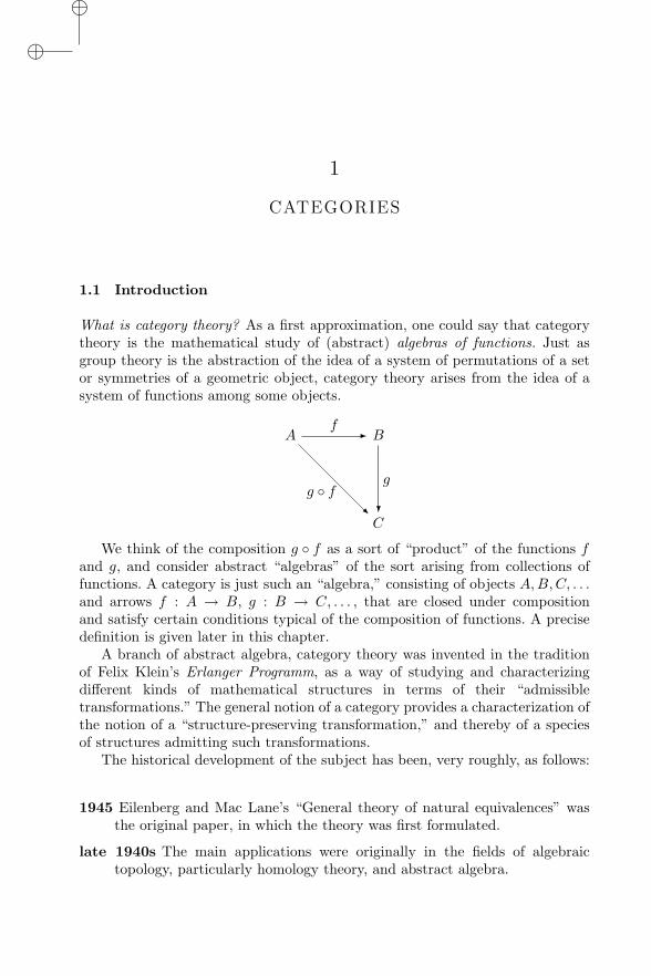
What is category theory? As a first approximation, one could say that categorytheory is the mathematical study of (abstract) algebras of functions. Just asgroup theory is the abstraction of the idea of a system of permutations of a setor symmetries of a geometric object, category theory arises from the idea of asystem of functions among some objects.
Af - B
C
g
?g ◦ f
-
We think of the composition g ◦ f as a sort of “product” of the functions fand g, and consider abstract “algebras” of the sort arising from collections offunctions. A category is just such an “algebra,” consisting of objects A,B,C, . . .and arrows f : A → B, g : B → C, . . . , that are closed under compositionand satisfy certain conditions typical of the composition of functions. A precisedefinition is given later in this chapter.
A branch of abstract algebra, category theory was invented in the traditionof Felix Klein’s Erlanger Programm, as a way of studying and characterizingdifferent kinds of mathematical structures in terms of their “admissibletransformations.” The general notion of a category provides a characterization ofthe notion of a “structure-preserving transformation,” and thereby of a speciesof structures admitting such transformations.
The historical development of the subject has been, very roughly, as follows:
1945 Eilenberg and Mac Lane’s “General theory of natural equivalences” wasthe original paper, in which the theory was first formulated.
late 1940s The main applications were originally in the fields of algebraictopology, particularly homology theory, and abstract algebra.
“chap01”2009/2/4page 2i
ii
i
ii
ii
2 CATEGORIES
1950s A. Grothendieck et al. began using category theory with great success inalgebraic geometry.
1960s F.W. Lawvere and others began applying categories to logic, revealingsome deep and surprising connections.
1970s Applications were already appearing in computer science, linguistics,cognitive science, philosophy, and many other areas.
One very striking thing about the field is that it has such wide-rangingapplications. In fact, it turns out to be a kind of universal mathematicallanguage like set theory. As a result of these various applications, category theoryalso tends to reveal certain connections between different fields—like logic andgeometry. For example, the important notion of an adjoint functor occurs inlogic as the existential quantifier and in topology as the image operation alonga continuous function. From a categorical point of view these turn out to beessentially the same operation.
The concept of adjoint functor is in fact one of the main things that the readershould take away from the study of this book. It is a strictly category-theoreticalnotion that has turned out to be a conceptual tool of the first magnitude—onpar with the idea of a continuous function.
In fact, just as the idea of a topological space arose in connection withcontinuous functions, so also the notion of a category arose in order to definethat of a functor, at least according to one of the inventors. The notion of afunctor arose—so the story goes on—in order to define natural transformations.One might as well continue that natural transformations serve to define adjoints:
CategoryFunctor
Natural transformationAdjunction
Indeed, that gives a pretty good outline of this book.Before getting down to business, let us ask why it should be that category
theory has such far-reaching applications. Well, we said that it is the abstracttheory of functions, so the answer is simply this:
Functions are everywhere!
And everywhere that functions are, there are categories. Indeed, the subjectmight better have been called abstract function theory, or, perhaps even better:archery.
“chap01”2009/2/4page 3i
ii
i
ii
ii
FUNCTIONS OF SETS 3
1.2 Functions of sets
We begin by considering functions between sets. I am not going to say here whata function is, anymore than what a set is. Instead, we will assume a workingknowledge of these terms. They can in fact be defined using category theory, butthat is not our purpose here.
Let f be a function from a set A to another set B, we write
f : A→ B.
To be explicit, this means that f is defined on all of A and all the values of fare in B. In set theoretic terms,
range(f) ⊆ B.
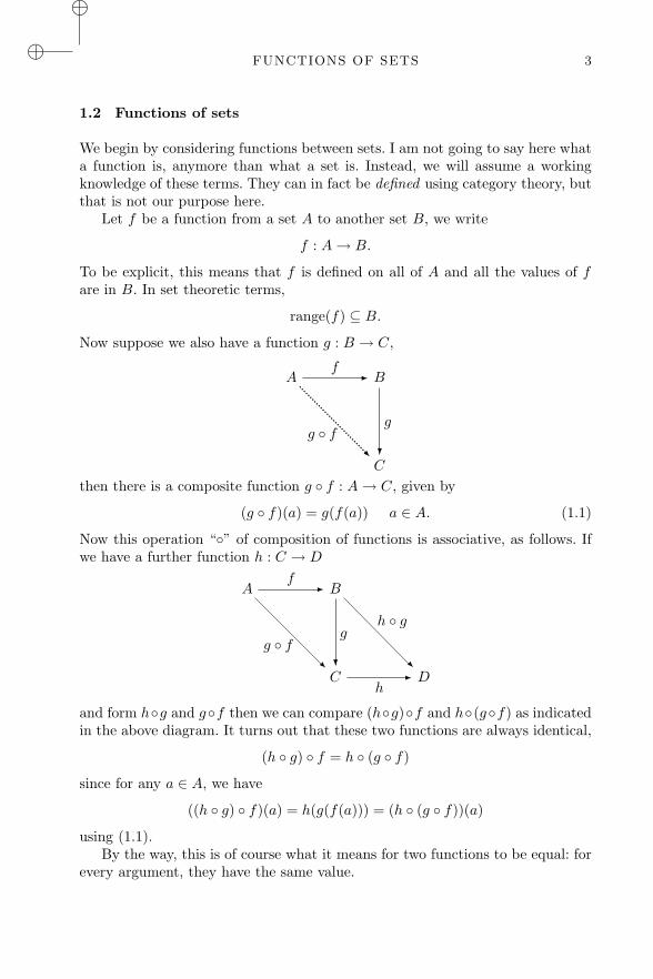
Now suppose we also have a function g : B → C,
Af - B
C
g
?g ◦ f
................................-
then there is a composite function g ◦ f : A→ C, given by
(g ◦ f)(a) = g(f(a)) a ∈ A. (1.1)
Now this operation “◦” of composition of functions is associative, as follows. Ifwe have a further function h : C → D
Af - B
C
g
?
h-
g ◦ f-
D
h ◦ g
-
and form h◦g and g◦f then we can compare (h◦g)◦f and h◦(g◦f) as indicatedin the above diagram. It turns out that these two functions are always identical,
(h ◦ g) ◦ f = h ◦ (g ◦ f)
since for any a ∈ A, we have
((h ◦ g) ◦ f)(a) = h(g(f(a))) = (h ◦ (g ◦ f))(a)
using (1.1).By the way, this is of course what it means for two functions to be equal: for
every argument, they have the same value.
“chap01”2009/2/4page 4i
ii
i
ii
ii
4 CATEGORIES
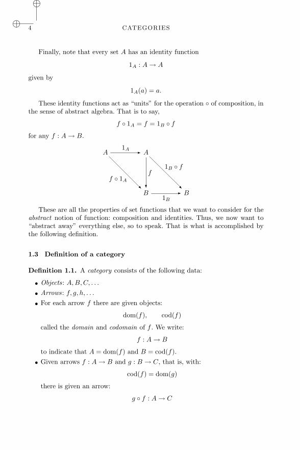
Finally, note that every set A has an identity function
1A : A→ A
given by
1A(a) = a.
These identity functions act as “units” for the operation ◦ of composition, inthe sense of abstract algebra. That is to say,
f ◦ 1A = f = 1B ◦ f
for any f : A→ B.
A1A - A
B
f
?
1B
-
f ◦ 1A -
B
1B ◦ f
-
These are all the properties of set functions that we want to consider for theabstract notion of function: composition and identities. Thus, we now want to“abstract away” everything else, so to speak. That is what is accomplished bythe following definition.
1.3 Definition of a category
Definition 1.1. A category consists of the following data:
• Objects: A,B,C, . . .
• Arrows: f, g, h, . . .
• For each arrow f there are given objects:
dom(f), cod(f)
called the domain and codomain of f . We write:
f : A→ B
to indicate that A = dom(f) and B = cod(f).
• Given arrows f : A→ B and g : B → C, that is, with:
cod(f) = dom(g)
there is given an arrow:
g ◦ f : A→ C
“chap01”2009/2/4page 5i
ii
i
ii
ii
EXAMPLES OF CATEGORIES 5
called the composite of f and g.
• For each object A there is given an arrow:
1A : A→ A
called the identity arrow of A.
These data are required to satisfy the following laws:
• Associativity:
h ◦ (g ◦ f) = (h ◦ g) ◦ f
for all f : A→ B, g : B → C, h : C → D.
• Unit:
f ◦ 1A = f = 1B ◦ f
for all f : A→ B.
A category is anything that satisfies this definition—and we will have plenty ofexamples very soon. For now I want to emphasize that, unlike in the previoussection, the objects do not have to be sets and the arrows need not be functions. Inthis sense, a category is an abstract algebra of functions, or “arrows” (sometimesalso called “morphisms”), with the composition operation “◦” as primitive. If youare familiar with groups, you may think of a category as a sort of generalized group.
1.4 Examples of categories
1. We have already encountered the category Sets of sets and functions.There is also the category
Setsfin
of all finite sets and functions between them.Indeed, there are many categories like this, given by restricting the setsthat are to be the objects and the functions that are to be the arrows.For example, take finite sets as objects and injective (i.e., “1 to 1”)functions as arrows. Since injective functions compose to give an injectivefunction, and since the identity functions are injective, this also givesa category.
What if we take sets as objects and as arrows, those f : A → B suchthat for all b ∈ B, the subset
f−1(b) ⊆ A
has at most two elements (rather than one)? Is this still a category? Whatif we take the functions such that f−1(b) is finite? infinite? There are lotsof such restricted categories of sets and functions.
“chap01”2009/2/4page 6i
ii
i
ii
ii
6 CATEGORIES
2. Another kind of example one often sees in mathematics is categoriesof structured sets, that is, sets with some further “structure” andfunctions which “preserve it,” where these notions are determined in someindependent way. Examples of this kind you may be familiar with are:
• groups and group homomorphisms,
• vector spaces and linear mappings,
• graphs and graph homomorphisms,
• the real numbers R and continuous functions R→ R,
• open subsets U ⊆ R and continuous functions f : U → V ⊆ R definedon them,
• topological spaces and continuous mappings,
• differentiable manifolds and smooth mappings,
• the natural numbers N and all recursive functions N → N, or as inthe example of continuous functions, one can take partial recursivefunctions defined on subsets U ⊆ N.
• posets and monotone functions.
Do not worry if some of these examples are unfamiliar to you. Later on,we will take a closer look at some of them. For now, let us just considerthe last of the above examples in more detail.
3. A partially ordered set or poset is a set A equipped with a binary relationa ≤A b such that the following conditions hold for all a, b, c ∈ A:
reflexivity: a ≤A a,transitivity: if a ≤A b and b ≤A c, then a ≤A c,antisymmetry: if a ≤A b and b ≤A a, then a = b.
For example, the real numbers R with their usual ordering x ≤ y form aposet that is also linearly ordered: either x ≤ y or y ≤ x for any x, y.
An arrow from a poset A to a poset B is a function
m : A→ B
that is monotone, in the sense that, for all a, a′ ∈ A,
a ≤A a′ implies m(a) ≤B m(a′).
What does it take for this to be a category? We need to know that 1A :A → A is monotone, but that is clear since a ≤A a′ implies a ≤A a′.We also need to know that if f : A → B and g : B → C are monotone,then g ◦ f : A → C is monotone. This also holds, since a ≤ a′ impliesf(a) ≤ f(a′) implies g(f(a)) ≤ g(f(a′)) implies (g ◦ f)(a) ≤ (g ◦ f)(a′). Sowe have the category Pos of posets and monotone functions.
“chap01”2009/2/4page 7i
ii
i
ii
ii
EXAMPLES OF CATEGORIES 7
4. The categories that we have been considering so far are examples of whatare sometimes called concrete categories. Informally, these are categoriesin which the objects are sets, possibly equipped with some structure, andthe arrows are certain, possibly structure-preserving, functions (we shallsee later on that this notion is not entirely coherent; see Remark 1.7).But in fact, one way of understanding what category theory is all aboutis “doing without elements”, and replacing them by arrows instead. Letus now take a look at some examples where this point of view is not justoptional, but essential.Let Rel be the following category: take sets as objects and take binaryrelations as arrows. That is, an arrow f : A → B is an arbitrary subsetf ⊆ A×B. The identity arrow on a set A is the identity relation.
1A = {(a, a) ∈ A×A | a ∈ A} ⊆ A×A.
Given R ⊆ A×B and S ⊆ B × C, define composition S ◦R by
(a, c) ∈ S ◦R iff ∃b. (a, b) ∈ R & (b, c) ∈ S
that is, the “relative product” of S and R. We leave it as an exercise toshow that Rel is in fact a category. (What needs to be done?)
For another example of a category in which the arrows are not“functions,” let the objects be finite sets A,B,C and an arrow F : A→ Bis a rectangular matrix F = (nij)i<a,j<b of natural numbers with a = |A|and b = |B|, where |C| is the number of elements in a set C. Thecomposition of arrows is by the usual matrix multiplication, and theidentity arrows are the usual unit matrices. The objects here are servingsimply to ensure that the matrix multiplication is defined, but the matricesare not functions between them.
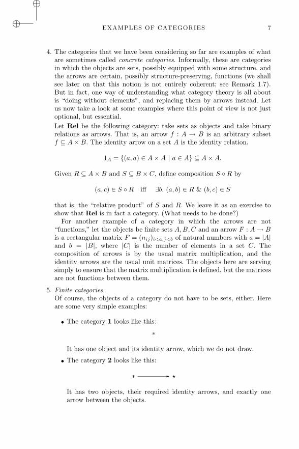
5. Finite categoriesOf course, the objects of a category do not have to be sets, either. Hereare some very simple examples:
• The category 1 looks like this:
∗
It has one object and its identity arrow, which we do not draw.
• The category 2 looks like this:
∗ - ?
It has two objects, their required identity arrows, and exactly onearrow between the objects.
“chap01”2009/2/4page 8i
ii
i
ii
ii
8 CATEGORIES
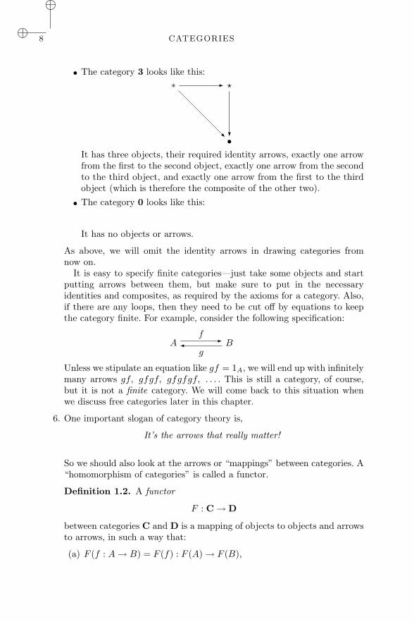
• The category 3 looks like this:∗ - ?
•?
-
It has three objects, their required identity arrows, exactly one arrowfrom the first to the second object, exactly one arrow from the secondto the third object, and exactly one arrow from the first to the thirdobject (which is therefore the composite of the other two).
• The category 0 looks like this:
It has no objects or arrows.
As above, we will omit the identity arrows in drawing categories fromnow on.
It is easy to specify finite categories—just take some objects and startputting arrows between them, but make sure to put in the necessaryidentities and composites, as required by the axioms for a category. Also,if there are any loops, then they need to be cut off by equations to keepthe category finite. For example, consider the following specification:
Af -�g
B
Unless we stipulate an equation like gf = 1A, we will end up with infinitelymany arrows gf, gfgf, gfgfgf, . . . . This is still a category, of course,but it is not a finite category. We will come back to this situation whenwe discuss free categories later in this chapter.
6. One important slogan of category theory is,
It’s the arrows that really matter!
So we should also look at the arrows or “mappings” between categories. A“homomorphism of categories” is called a functor.
Definition 1.2. A functor
F : C→ D
between categories C and D is a mapping of objects to objects and arrowsto arrows, in such a way that:
(a) F (f : A→ B) = F (f) : F (A)→ F (B),
“chap01”2009/2/4page 9i
ii
i
ii
ii
EXAMPLES OF CATEGORIES 9
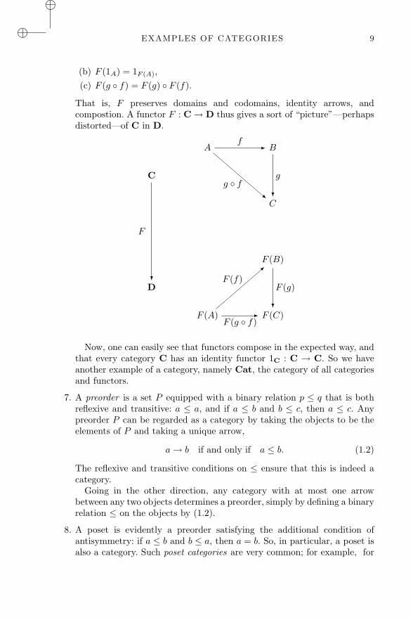
(b) F (1A) = 1F (A),(c) F (g ◦ f) = F (g) ◦ F (f).
That is, F preserves domains and codomains, identity arrows, andcompostion. A functor F : C→ D thus gives a sort of “picture”—perhapsdistorted—of C in D.
Af - B
C
C
g
?g ◦ f
-
F (B)
D
F
?
F (A)F (g ◦ f)
-
F (f)-
F (C)
F (g)
?
Now, one can easily see that functors compose in the expected way, andthat every category C has an identity functor 1C : C → C. So we haveanother example of a category, namely Cat, the category of all categoriesand functors.
7. A preorder is a set P equipped with a binary relation p ≤ q that is bothreflexive and transitive: a ≤ a, and if a ≤ b and b ≤ c, then a ≤ c. Anypreorder P can be regarded as a category by taking the objects to be theelements of P and taking a unique arrow,
a→ b if and only if a ≤ b. (1.2)
The reflexive and transitive conditions on ≤ ensure that this is indeed acategory.
Going in the other direction, any category with at most one arrowbetween any two objects determines a preorder, simply by defining a binaryrelation ≤ on the objects by (1.2).
8. A poset is evidently a preorder satisfying the additional condition ofantisymmetry: if a ≤ b and b ≤ a, then a = b. So, in particular, a poset isalso a category. Such poset categories are very common; for example, for
“chap01”2009/2/4page 10i
ii
i
ii
ii
10 CATEGORIES
any set X, the powerset P(X) is a poset under the usual inclusion relationU ⊆ V between the subsets U, V of X.
What is a functor F : P → Q between poset categories P and Q? Itmust satisfy the identity and composition laws . . . . Clearly, these are justthe monotone functions already considered above.It is often useful to think of a category as a kind of generalized poset,one with “more structure” than just p ≤ q. Thus, one can also think of afunctor as a generalized monotone map.
9. An example from topology: Let X be a topological space with collection ofopen sets O(X). Ordered by inclusion, O(X) is a poset category. Moreover,the points of X can be preordered by specialization by setting x ≤ y iffx ∈ U implies y ∈ U for every open set U , i.e. y is contained in every openset that contains x. If X is sufficiently separated (“T1”), then this orderingbecomes trivial, but it can be quite interesting otherwise, as happensin the spaces of algebraic geometry and denotational semantics. It is anexercise to show that T0 spaces are actually posets under the specializationordering.
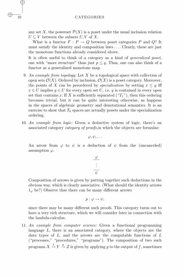
10. An example from logic: Given a deductive system of logic, there’s anassociated category category of proofs,in which the objects are formulas:
ϕ,ψ, . . .
An arrow from ϕ to ψ is a deduction of ψ from the (uncanceled)assumption ϕ.
ϕ
...
ψ
Composition of arrows is given by putting together such deductions in theobvious way, which is clearly associative. (What should the identity arrows1ϕ be?) Observe that there can be many different arrows
p : ϕ→ ψ,
since there may be many different such proofs. This category turns out tohave a very rich structure, which we will consider later in connection withthe lambda-calculus.
11. An example from computer science: Given a functional programminglanguage L, there is an associated category, where the objects are thedata types of L, and the arrows are the computable functions of L(“processes,” “procedures,” “programs”). The composition of two such
programs Xf→ Y
g→ Z is given by applying g to the output of f , sometimes
“chap01”2009/2/4page 11i
ii
i
ii
ii
EXAMPLES OF CATEGORIES 11
also written
g ◦ f = f ; g.
The identity is the “do nothing” program.Categories such as this are basic to the idea of denotational semantics of
programming languages. For example, if C(L) is the category just defined,then the denotational semantics of the language L in a category D of, say,Scott domains is simply a functor
S : C(L)→ D
since S assigns domains to the types of L and continuous functions tothe programs. Both this example and the previous one are related to thenotion of “cartesian closed category” that is considered later.
12. Let X be a set. We can regard X as a category Dis(X) by taking theobjects to be the elements of X and taking the arrows to be just therequired identity arrows, one for each x ∈ X. Such categories, in which theonly arrows are identities, are called discrete. Note that discrete categoriesare just very special posets.
13. A monoid (sometimes called a semigroup with unit) is a set M equippedwith a binary operation · : M × M → M and a distinguished “unit”element u ∈M such that for all x, y, z ∈M ,
x · (y · z) = (x · y) · z
and
u · x = x = x · u.
Equivalently, a monoid is a category with just one object. The arrows ofthe category are the elements of the monoid. In particular, the identityarrow is the unit element u. Composition of arrows is the binary operationm · n of the monoid.
Monoids are very common: there are the monoids of numbers like N, Qor R with addition and 0, or multiplication and 1. But also for any set X,the set of functions from X to X, written
HomSets(X,X)
is a monoid under the operation of composition. More generally, for anyobject C in any category C, the set of arrows from C to C, written asHomC(C,C), is a monoid under the composition operation of C.
Since monoids are structured sets, there is a category Mon whoseobjects are monoids and whose arrows are functions that preserve themonoid structure. In detail, a homomorphism from a monoid M to amonoid N is a function h : M → N such that for all m,n ∈M ,
h(m ·M n) = h(m) ·N h(n)
“chap01”2009/2/4page 12i
ii
i
ii
ii
12 CATEGORIES
and
h(uM ) = uN .
Observe that a monoid homomorphism from M to N is the same thingas a functor from M regarded as a category to N regarded as a category.In this sense, categories are also generalized monoids, and functors aregeneralized homomorphisms.
1.5 Isomorphisms
Definition 1.3. In any category C, an arrow f : A → B is called anisomorphism if there is an arrow g : B → A in C such that
g ◦ f = 1A and f ◦ g = 1B .
Since inverses are unique (proof!), we write g = f−1. We say that A is isomorphicto B, written A ∼= B, if there exists an isomorphism between them.
The definition of isomorphism is our first example of an abstract, categorytheoretic definition of an important notion. It is abstract in the sense that itmakes use only of the category theoretic notions, rather than some additionalinformation about the objects and arrows. It has the advantage over otherpossible definitions that it applies in any category. For example, one sometimesdefines an isomorphism of sets (monoids, etc.) as a bijective function (resp.homomorphism), i.e., one that is “1-1 and onto”—making use of the elements ofthe objects. This is equivalent to our definition in some cases, such as sets andmonoids. But note that, for example in Pos, the category theoretic definitiongives the right notion, while there are “bijective homomorphisms” between non-isomorphic posets. Moreover, in many cases only the abstract definition makessense, as for example, in the case of a monoid regarded as a category.
Definition 1.4. A group G is a monoid with an inverse g−1 for every element g.Thus G is a category with one object, in which every arrow is an isomorphism.
The natural numbers N do not form a group under either addition ormultiplication, but the integers Z and the positive rationals Q+, respectively, do.For any set X, we have the group Aut(X) of automorphisms (or “permutations”)of X, that is, isomorphisms f : X → X. (Why is this closed under “◦”?) A groupof permutations is a subgroup G ⊆ Aut(X) for some set X, that is, a group of(some) automorphisms of X. Thus the set G must satisfy the following:
1. The identity function 1X on X is in G.2. If g, g′ ∈ G, then g ◦ g′ ∈ G.3. If g ∈ G, then g−1 ∈ G.
“chap01”2009/2/4page 13i
ii
i
ii
ii
ISOMORPHISMS 13
A homomorphism of groups h : G→ H is just a homomorphism of monoids,which then necessarily also preserves the inverses (proof!).
Now consider the following basic, classical result about abstract groups:
Theorem (Cayley). Every group G is isomorphic to a group of permutations.
Proof. (sketch)
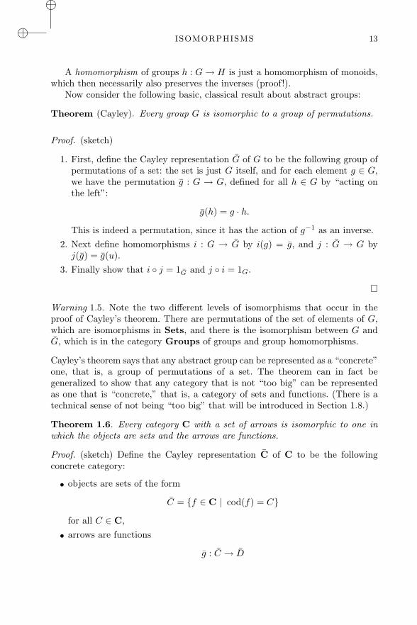
1. First, define the Cayley representation G of G to be the following group ofpermutations of a set: the set is just G itself, and for each element g ∈ G,we have the permutation g : G → G, defined for all h ∈ G by “acting onthe left”:
g(h) = g · h.
This is indeed a permutation, since it has the action of g−1 as an inverse.2. Next define homomorphisms i : G → G by i(g) = g, and j : G → G byj(g) = g(u).
3. Finally show that i ◦ j = 1G and j ◦ i = 1G.
Warning 1.5. Note the two different levels of isomorphisms that occur in theproof of Cayley’s theorem. There are permutations of the set of elements of G,which are isomorphisms in Sets, and there is the isomorphism between G andG, which is in the category Groups of groups and group homomorphisms.
Cayley’s theorem says that any abstract group can be represented as a “concrete”one, that is, a group of permutations of a set. The theorem can in fact begeneralized to show that any category that is not “too big” can be representedas one that is “concrete,” that is, a category of sets and functions. (There is atechnical sense of not being “too big” that will be introduced in Section 1.8.)
Theorem 1.6. Every category C with a set of arrows is isomorphic to one inwhich the objects are sets and the arrows are functions.
Proof. (sketch) Define the Cayley representation C of C to be the followingconcrete category:
• objects are sets of the form
C = {f ∈ C | cod(f) = C}
for all C ∈ C,
• arrows are functions
g : C → D
“chap01”2009/2/4page 14i
ii
i
ii
ii
14 CATEGORIES
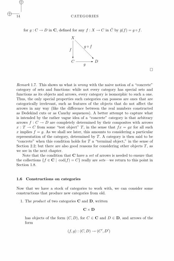
for g : C → D in C, defined for any f : X → C in C by g(f) = g ◦ f .
X
C
f
?
g- D
g ◦ f
-
Remark 1.7. This shows us what is wrong with the naive notion of a “concrete”category of sets and functions: while not every category has special sets andfunctions as its objects and arrows, every category is isomorphic to such a one.Thus, the only special properties such categories can possess are ones that arecategorically irrelevant, such as features of the objects that do not affect thearrows in any way (like the difference between the real numbers constructedas Dedekind cuts or as Cauchy sequences). A better attempt to capture whatis intended by the rather vague idea of a “concrete” category is that arbitraryarrows f : C → D are completely determined by their composites with arrowsx : T → C from some “test object” T , in the sense that fx = gx for all suchx implies f = g. As we shall see later, this amounts to considering a particularrepresentation of the category, determined by T . A category is then said to be“concrete” when this condition holds for T a “terminal object,” in the sense ofSection 2.2; but there are also good reasons for considering other objects T , aswe see in the next chapter.
Note that the condition that C have a set of arrows is needed to ensure thatthe collections {f ∈ C | cod(f) = C} really are sets—we return to this point inSection 1.8.
1.6 Constructions on categories
Now that we have a stock of categories to work with, we can consider someconstructions that produce new categories from old.
1. The product of two categories C and D, written
C×D
has objects of the form (C,D), for C ∈ C and D ∈ D, and arrows of theform
(f, g) : (C,D)→ (C ′, D′)
“chap01”2009/2/4page 15i
ii
i
ii
ii
CONSTRUCTIONS ON CATEGORIES 15
for f : C → C ′ ∈ C and g : D → D′ ∈ D. Composition and units aredefined componentwise; that is,
(f ′, g′) ◦ (f, g) = (f ′ ◦ f, g′ ◦ g)
1(C,D) = (1C , 1D).
There are two obvious projection functors
C �π1 C×D
π2- D
defined by π1(C,D) = C and π1(f, g) = f , and similarly for π2.The reader familiar with groups will recognize that for groups G and H,
the product category G×H is the usual (direct) product of groups.
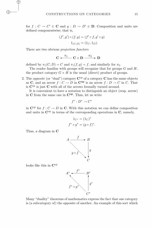
2. The opposite (or “dual”) category Cop of a category C has the same objectsas C, and an arrow f : C → D in Cop is an arrow f : D → C in C. Thatis Cop is just C with all of the arrows formally turned around.
It is convenient to have a notation to distinguish an object (resp. arrow)in C from the same one in Cop. Thus, let us write
f∗ : D∗ → C∗
in Cop for f : C → D in C. With this notation we can define compositionand units in Cop in terms of the corresponding operations in C, namely,
1C∗ = (1C)∗
f∗ ◦ g∗ = (g ◦ f)∗.
Thus, a diagram in C
Af - B
C
g
?g ◦ f
-
looks like this in Cop
A∗ �f∗
B∗
C∗
g∗
6
f∗ ◦ g∗
�
Many “duality” theorems of mathematics express the fact that one categoryis (a subcategory of) the opposite of another. An example of this sort which
“chap01”2009/2/4page 16i
ii
i
ii
ii
16 CATEGORIES
we will prove later is that Sets is dual to the category of complete, atomicBoolean algebras.
3. The arrow category C→ of a category C has the arrows of C as objects,and an arrow g from f : A→ B to f ′ : A′ → B′ in C→ is a “commutativesquare”
Ag1 - A′
B
f
?
g2
- B′
f ′
?
where g1 and g2 are arrows in C. That is, such an arrow is a pair of arrowsg = (g1, g2) in C such that
g2 ◦ f = f ′ ◦ g1.
The identity arrow 1f on an object f : A → B is the pair (1A, 1B).Composition of arrows is done componentwise:
(h1, h2) ◦ (g1, g2) = (h1 ◦ g1, h2 ◦ g2)
The reader should verify that this works out by drawing the appropriatecommutative diagram.
Observe that there are two functors:
C �dom
C→cod- C
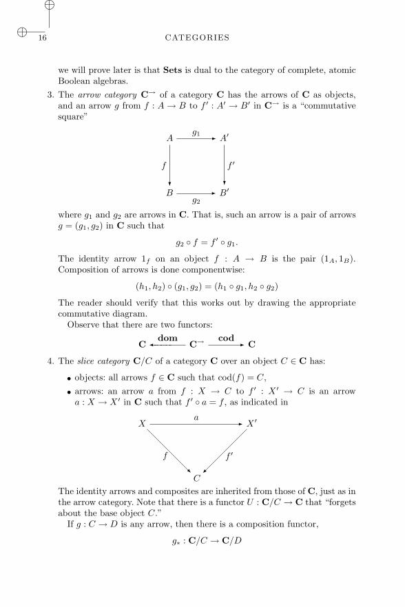
4. The slice category C/C of a category C over an object C ∈ C has:
• objects: all arrows f ∈ C such that cod(f) = C,
• arrows: an arrow a from f : X → C to f ′ : X ′ → C is an arrowa : X → X ′ in C such that f ′ ◦ a = f , as indicated in
Xa - X ′
C
f ′
�
f-
The identity arrows and composites are inherited from those of C, just as inthe arrow category. Note that there is a functor U : C/C → C that “forgetsabout the base object C.”
If g : C → D is any arrow, then there is a composition functor,
g∗ : C/C → C/D
“chap01”2009/2/4page 17i
ii
i
ii
ii
CONSTRUCTIONS ON CATEGORIES 17
defined by g∗(f) = g ◦ f ,X
C
f
?
g- D
g ◦ f
-
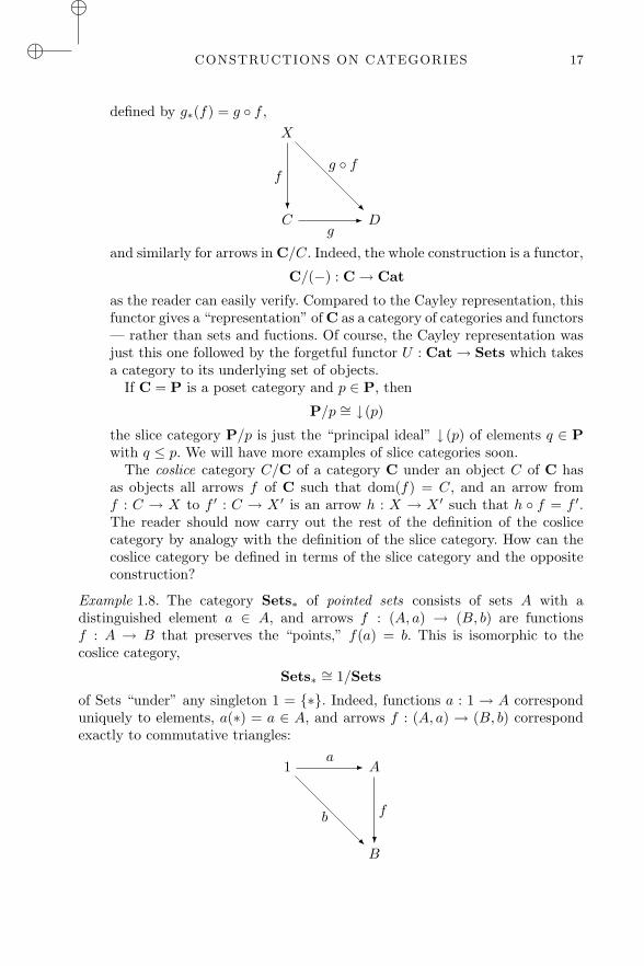
and similarly for arrows in C/C. Indeed, the whole construction is a functor,
C/(−) : C→ Cat
as the reader can easily verify. Compared to the Cayley representation, thisfunctor gives a “representation” of C as a category of categories and functors— rather than sets and fuctions. Of course, the Cayley representation wasjust this one followed by the forgetful functor U : Cat→ Sets which takesa category to its underlying set of objects.
If C = P is a poset category and p ∈ P, then
P/p ∼= ↓(p)
the slice category P/p is just the “principal ideal” ↓ (p) of elements q ∈ Pwith q ≤ p. We will have more examples of slice categories soon.
The coslice category C/C of a category C under an object C of C hasas objects all arrows f of C such that dom(f) = C, and an arrow fromf : C → X to f ′ : C → X ′ is an arrow h : X → X ′ such that h ◦ f = f ′.The reader should now carry out the rest of the definition of the coslicecategory by analogy with the definition of the slice category. How can thecoslice category be defined in terms of the slice category and the oppositeconstruction?
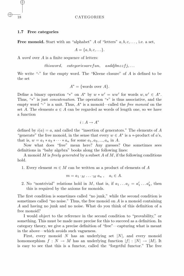
Example 1.8. The category Sets∗ of pointed sets consists of sets A with adistinguished element a ∈ A, and arrows f : (A, a) → (B, b) are functionsf : A → B that preserves the “points,” f(a) = b. This is isomorphic to thecoslice category,
Sets∗ ∼= 1/Sets
of Sets “under” any singleton 1 = {∗}. Indeed, functions a : 1 → A corresponduniquely to elements, a(∗) = a ∈ A, and arrows f : (A, a) → (B, b) correspondexactly to commutative triangles:
1a - A
B
f
?
b-
“chap01”2009/2/4page 18i
ii
i
ii
ii
18 CATEGORIES
1.7 Free categories
Free monoid. Start with an “alphabet” A of “letters” a, b, c, . . . , i.e. a set,
A = {a, b, c, . . .}.
A word over A is a finite sequence of letters:
thisword, categoriesarefun, asddjbnzzfj, . . .
We write “-” for the empty word. The “Kleene closure” of A is defined to bethe set
A∗ = {words over A}.
Define a binary operation “∗” on A∗ by w ∗ w′ = ww′ for words w,w′ ∈ A∗.Thus, “∗” is just concatenation. The operation “∗” is thus associative, and theempty word “-” is a unit. Thus, A∗ is a monoid—called the free monoid on theset A. The elements a ∈ A can be regarded as words of length one, so we havea function
i : A→ A∗
defined by i(a) = a, and called the “insertion of generators.” The elements of A“generate” the free monoid, in the sense that every w ∈ A∗ is a ∗-product of a’s,that is, w = a1 ∗ a2 ∗ · · · ∗ an for some a1, a2, ..., an in A.
Now what does “free” mean here? Any guesses? One sometimes seesdefinitions in “baby algebra” books along the following lines:
A monoid M is freely generated by a subset A of M , if the following conditionshold.
1. Every element m ∈M can be written as a product of elements of A
m = a1 ·M . . . ·M an , ai ∈ A.
2. No “nontrivial” relations hold in M , that is, if a1 . . . aj = a′1 . . . a′k, then
this is required by the axioms for monoids.
The first condition is sometimes called “no junk,” while the second condition issometimes called “no noise.” Thus, the free monoid on A is a monoid containingA and having no junk and no noise. What do you think of this definition of afree monoid?
I would object to the reference in the second condition to “provability,” orsomething. This must be made more precise for this to succeed as a definition. Incategory theory, we give a precise definition of “free”—capturing what is meantin the above—which avoids such vagueness.
First, every monoid N has an underlying set |N |, and every monoidhomomorphism f : N → M has an underlying function |f | : |N | → |M |. Itis easy to see that this is a functor, called the “forgetful functor.” The free
“chap01”2009/2/4page 19i
ii
i
ii
ii
FREE CATEGORIES 19
monoid M(A) on a set A is by definition “the” monoid with the following socalled universal mapping property, or UMP!
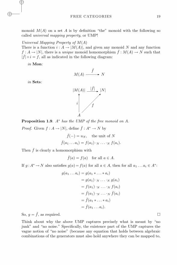
Universal Mapping Property of M(A)There is a function i : A→ |M(A)|, and given any monoid N and any functionf : A→ |N |, there is a unique monoid homomorphism f : M(A)→ N such that|f | ◦ i = f , all as indicated in the following diagram:
in Mon:
M(A) ...............f- N
in Sets:
|M(A)| |f |- |N |
A
i
6
f
-
Proposition 1.9. A∗ has the UMP of the free monoid on A.
Proof. Given f : A→ |N |, define f : A∗ → N by
f(−) = uN , the unit of N
f(a1 . . . ai) = f(a1) ·N . . . ·N f(ai).
Then f is clearly a homomorphism with
f(a) = f(a) for all a ∈ A.
If g :A∗→N also satisfies g(a) = f(a) for all a ∈ A, then for all a1 . . . ai ∈ A∗:
g(a1 . . . ai) = g(a1 ∗ . . . ∗ ai)
= g(a1) ·N . . . ·N g(ai)
= f(a1) ·N . . . ·N f(ai)
= f(a1) ·N . . . ·N f(ai)
= f(a1 ∗ . . . ∗ ai)
= f(a1 . . . ai).
So, g = f , as required.
Think about why the above UMP captures precisely what is meant by “nojunk” and “no noise.” Specifically, the existence part of the UMP captures thevague notion of “no noise” (because any equation that holds between algebraiccombinations of the generators must also hold anywhere they can be mapped to,
“chap01”2009/2/4page 20i
ii
i
ii
ii
20 CATEGORIES
and thus everywhere), while the uniqueness part makes precise the “no junk”idea (because any extra elements not combined from the generators would befree to be mapped to different values).
Using the UMP, it is easy to show that the free monoid M(A) is determineduniquely up to isomorphism, in the following sense.
Proposition 1.10. Given monoids M and N with functions i :A→|M | andj :A → |N |, each with the UMP of the free monoid on A, there is a (unique)monoid isomorphism h : M ∼= N such that |h|i = j and |h−1|j = i.
Proof. From j and the UMP of M , we have j : M → N with |j|i = j and fromi and the UMP of N , we have i : N → M with |i|j = i. Composing gives ahomomorphism i ◦ j : M → M such that |i ◦ j|i = i. Since 1M : M → M alsohas this property, by the uniqueness part of the UMP of M , we have i ◦ j = 1M .Exchanging the roles of M and N shows j ◦ i = 1N ;
in Mon:
M ...................j- N ...................
i- M
in Sets:
|M | |j|- |N ||i| - |M |
A
j
6
i
-
i
�
For example, the free monoid on any set with a single element is easilyseen to be isomorphic to the monoid of natural numbers N under addition (the“generator” is the number 1). Thus, as a monoid, N is uniquely determined upto isomorphism by the UMP of free monoids.
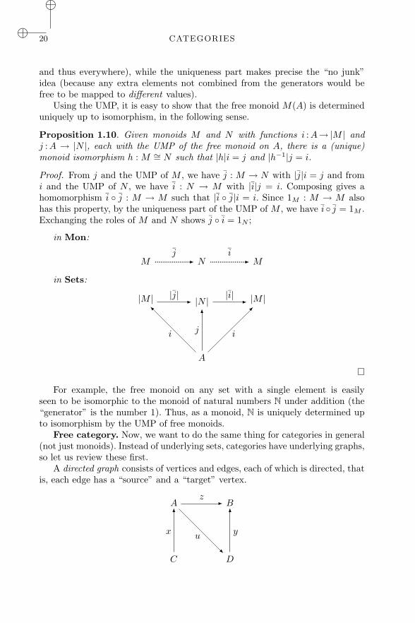
Free category. Now, we want to do the same thing for categories in general(not just monoids). Instead of underlying sets, categories have underlying graphs,so let us review these first.
A directed graph consists of vertices and edges, each of which is directed, thatis, each edge has a “source” and a “target” vertex.
Az - B
C
x
6
D
y
6
u-
“chap01”2009/2/4page 21i
ii
i
ii
ii
FREE CATEGORIES 21
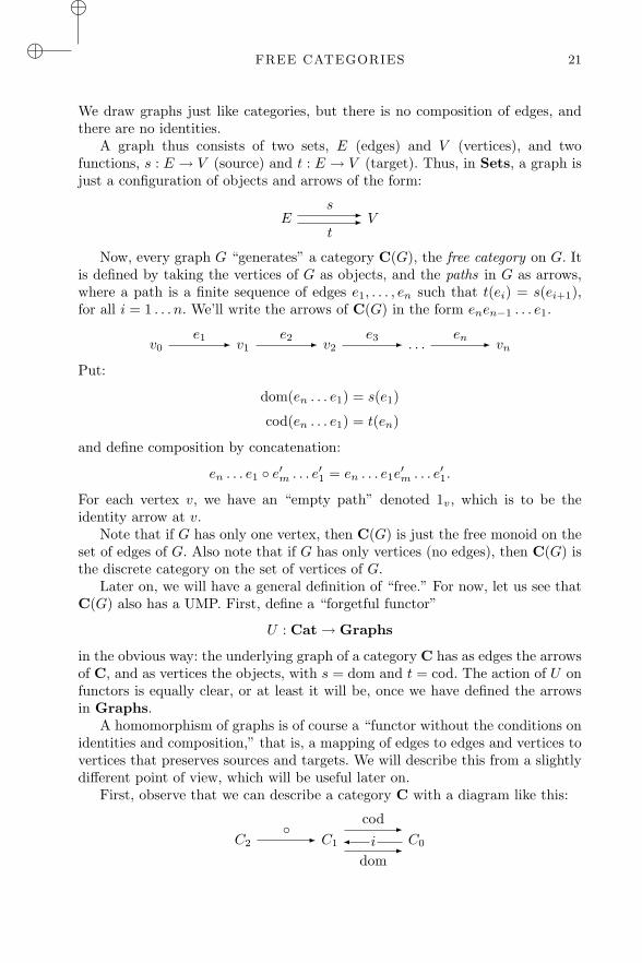
We draw graphs just like categories, but there is no composition of edges, andthere are no identities.
A graph thus consists of two sets, E (edges) and V (vertices), and twofunctions, s : E → V (source) and t : E → V (target). Thus, in Sets, a graph isjust a configuration of objects and arrows of the form:
Es -
t- V
Now, every graph G “generates” a category C(G), the free category on G. Itis defined by taking the vertices of G as objects, and the paths in G as arrows,where a path is a finite sequence of edges e1, . . . , en such that t(ei) = s(ei+1),for all i = 1 . . . n. We’ll write the arrows of C(G) in the form enen−1 . . . e1.
For each vertex v, we have an “empty path” denoted 1v, which is to be theidentity arrow at v.
Note that if G has only one vertex, then C(G) is just the free monoid on theset of edges of G. Also note that if G has only vertices (no edges), then C(G) isthe discrete category on the set of vertices of G.
Later on, we will have a general definition of “free.” For now, let us see thatC(G) also has a UMP. First, define a “forgetful functor”
U : Cat→ Graphs
in the obvious way: the underlying graph of a category C has as edges the arrowsof C, and as vertices the objects, with s = dom and t = cod. The action of U onfunctors is equally clear, or at least it will be, once we have defined the arrowsin Graphs.
A homomorphism of graphs is of course a “functor without the conditions onidentities and composition,” that is, a mapping of edges to edges and vertices tovertices that preserves sources and targets. We will describe this from a slightlydifferent point of view, which will be useful later on.
First, observe that we can describe a category C with a diagram like this:
C2◦ - C1
cod-� i
dom- C0
“chap01”2009/2/4page 22i
ii
i
ii
ii
22 CATEGORIES
where C0 is the collection of objects of C, C1 the arrows, i is the identity arrowoperation, and C2 is the collection {(f, g) ∈ C1 × C1 : cod(f) = dom(g)}.
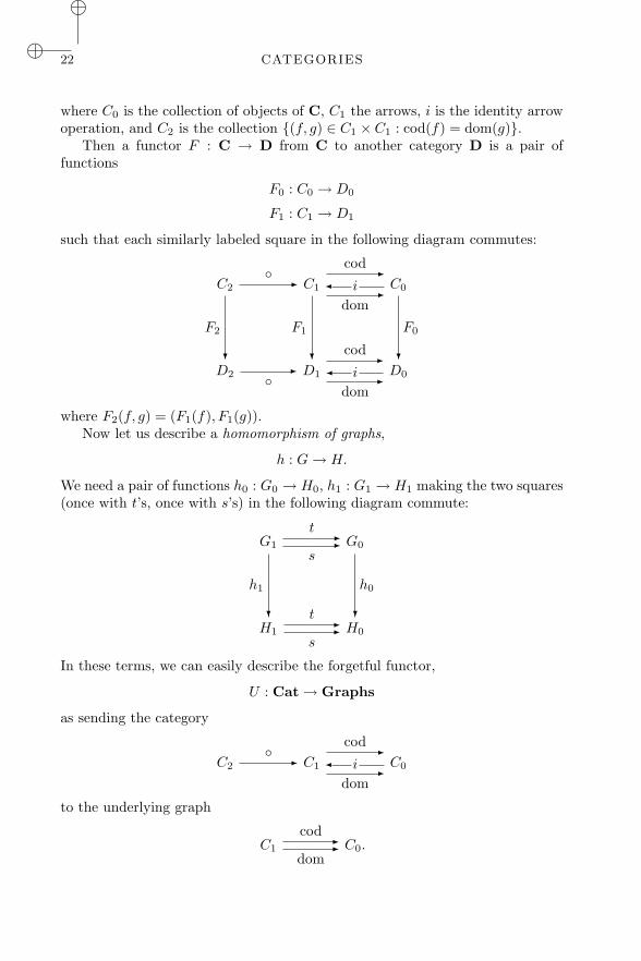
Then a functor F : C → D from C to another category D is a pair offunctions
F0 : C0 → D0
F1 : C1 → D1
such that each similarly labeled square in the following diagram commutes:
C2◦ - C1
cod-� i
dom- C0
D2
F2
?
◦- D1
F1
? cod-� i
dom- D0
F0
?
where F2(f, g) = (F1(f), F1(g)).Now let us describe a homomorphism of graphs,
h : G→ H.
We need a pair of functions h0 : G0 → H0, h1 : G1 → H1 making the two squares(once with t’s, once with s’s) in the following diagram commute:
G1
t -
s- G0
H1
h1
? t -
s- H0
h0
?
In these terms, we can easily describe the forgetful functor,
U : Cat→ Graphs
as sending the category
C2◦ - C1
cod-� i
dom- C0
to the underlying graph
C1
cod-dom- C0.
“chap01”2009/2/4page 23i
ii
i
ii
ii
FOUNDATIONS: LARGE, SMALL, AND LOCALLY SMALL 23
And similarly for functors, the effect of U is described by simply erasing someparts of the diagrams (which is easier to demonstrate with chalk!). Let us againwrite |C| = U(C), etc., for the underlying graph of a category C, in analogy tothe case of monoids above.
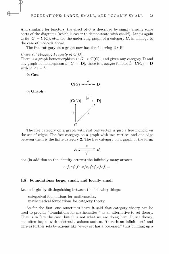
The free category on a graph now has the following UMP:
Universal Mapping Property of C(G)There is a graph homomorphism i : G→ |C(G)|, and given any category D andany graph homomorphism h : G→ |D|, there is a unique functor h : C(G)→ Dwith |h| ◦ i = h.
in Cat:
C(G) ................h- D
in Graph:
|C(G)||h|- |D|
G
i
6
h
-
The free category on a graph with just one vertex is just a free monoid onthe set of edges. The free category on a graph with two vertices and one edgebetween them is the finite category 2. The free category on a graph of the form:
Ae -
�f
B
has (in addition to the identity arrows) the infinitely many arrows:
e, f, ef, fe, efe, fef, efef, ...
1.8 Foundations: large, small, and locally small
Let us begin by distinguishing between the following things:
categorical foundations for mathematics,mathematical foundations for category theory.
As for the first: one sometimes hears it said that category theory can beused to provide “foundations for mathematics,” as an alternative to set theory.That is in fact the case, but it is not what we are doing here. In set theory,one often begins with existential axioms such as “there is an infinite set” andderives further sets by axioms like “every set has a powerset,” thus building up a
“chap01”2009/2/4page 24i
ii
i
ii
ii
24 CATEGORIES
universe of mathematical objects (namely sets), which in principle suffice for “allof mathematics.” Our axiom that every arrow has a domain and a codomain isnot to be understood in the same way as set theory’s axiom that every set has apowerset! The difference is that in set theory—at least as usually conceived—theaxioms are to be regarded as referring to (or determining) a single universe of sets.In category theory, by contrast, the axioms are a definition of something, namelyof categories. This is just like in group theory or topology, where the axioms serveto define the objects under investigation. These, in turn, are assumed to exist insome “background” or “foundational” system, like set theory (or type theory).That theory of sets could itself, in turn, be determined using category theory, orin some other way.
This brings us to the second point: we assume that our categories arecomprised of sets and functions, in one way or another, like most mathematicalobjects, and taking into account the remarks just made about the possibilityof categorical (or other) foundations. But in category theory, we sometimes runinto difficulties with set theory as usually practiced. Mostly these are questionsof size; some categories are “too big” to be handled comfortably in conventionalset theory.We already encountered this issue when we considered the Cayleyrepresentation in Section 1.5. There we had to require that the category underconsideration had (no more than) a set of arrows. We would certainly not want toimpose this restriction in general, however (as one usually does for, say, groups);for then even the “category” Sets would fail to be a proper category, as wouldmany other categories that we definitely want to study.
There are various formal devices for addressing these issues, and they arediscussed in the book by Mac Lane. For our immediate purposes, the followingdistinction will be useful:
Definition 1.11. A category C is called small if both the collection C0 ofobjects of C and the collection C1 of arrows of C are sets. Otherwise, C iscalled large.
For example, all finite categories are clearly small, as is the category Setsfin offinite sets and functions. (Actually, one should stipulate that the sets are onlybuilt from other finite sets, all the way down, i.e. that they are “hereditarilyfinite”.) On the other hand, the category Pos of posets, the category Groups ofgroups, and the category Sets of sets are all large. We let Cat be the categoryof all small categories, which itself is a large category. In particular, then, Catis not an object of itself, which may come as a relief to some readers.
This does not really solve all of our difficulties. Even for large categories likeGroups and Sets we will want to also consider constructions like the categoryof all functors from one to the other (we will define this “functor category”later). But if these are not small, conventional set theory does not provide themeans to do this directly (these categories would be “too large”). So, one needsa more elaborate theory of “classes” to handle such constructions. We will notworry about this when it is just a matter of technical foundations (Mac Lane I.6
“chap01”2009/2/4page 25i
ii
i
ii
ii
EXERCISES 25
addresses this issue). However, one very useful notion in this connection is thefollowing:
Definition 1.12. A category C is called locally small if for all objects X, Yin C, the collection HomC(X,Y ) = {f ∈ C1 | f : X → Y } is a set (called ahom-set).
Many of the large categories we want to consider are in fact locally small. Setsis locally small since HomSets(X,Y ) = Y X , the set of all functions from X to Y .Similarly, Pos, Top, and Group are all locally small (is Cat?), and, of course,any small category is locally small.
Warning 1.13. Don’t confuse the notions concrete and small. To say that acategory is concrete is to say that the objects of the category are (structured) sets,and the arrows of the category are (certain) functions. To say that a categoryis small is to say that the collection of all objects of the category is a set, as isthe collection of all arrows. The real numbers R, regarded as a poset category, issmall but not concrete. The category Pos of all posets is concrete but not small.
1.9 Exercises
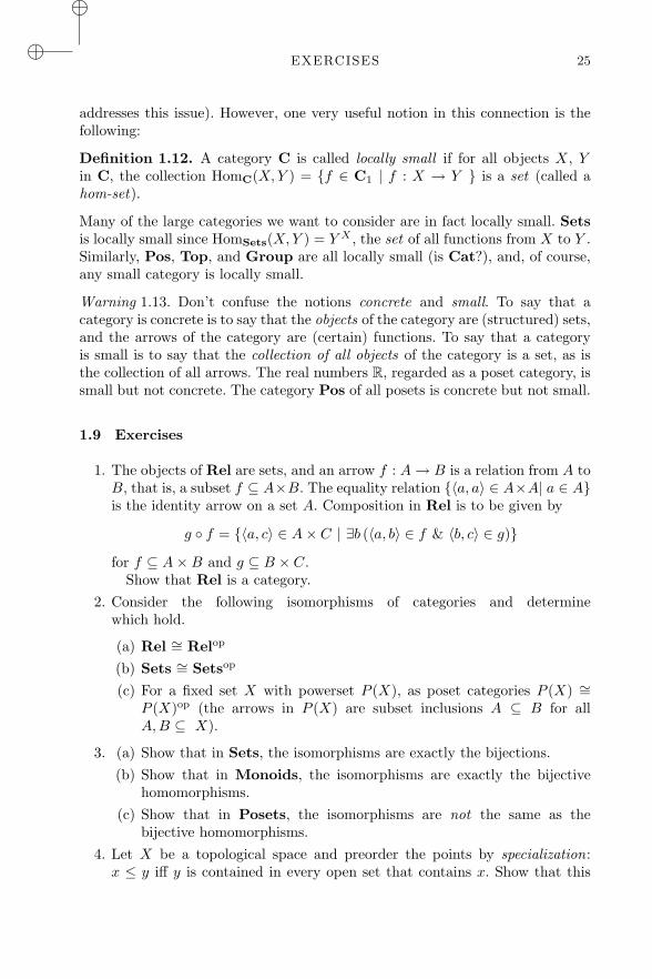
1. The objects of Rel are sets, and an arrow f : A→ B is a relation from A toB, that is, a subset f ⊆ A×B. The equality relation {〈a, a〉 ∈ A×A| a ∈ A}is the identity arrow on a set A. Composition in Rel is to be given by
g ◦ f = {〈a, c〉 ∈ A× C | ∃b (〈a, b〉 ∈ f & 〈b, c〉 ∈ g)}
for f ⊆ A×B and g ⊆ B × C.Show that Rel is a category.
2. Consider the following isomorphisms of categories and determinewhich hold.
(a) Rel ∼= Relop
(b) Sets ∼= Setsop
(c) For a fixed set X with powerset P (X), as poset categories P (X) ∼=P (X)op (the arrows in P (X) are subset inclusions A ⊆ B for allA,B ⊆ X).
3. (a) Show that in Sets, the isomorphisms are exactly the bijections.(b) Show that in Monoids, the isomorphisms are exactly the bijective
homomorphisms.(c) Show that in Posets, the isomorphisms are not the same as the
bijective homomorphisms.4. Let X be a topological space and preorder the points by specialization:x ≤ y iff y is contained in every open set that contains x. Show that this
“chap01”2009/2/4page 26i
ii
i
ii
ii
26 CATEGORIES
is a preorder, and that it is a poset if X is T0 (for any two distinct points,there is some open set containing one but not the other). Show that theordering is trivial if X is T1 (for any two distinct points, each is containedin an open set not containing the other).
5. For any category C, define a functor U : C/C → C from the slice categoryover an object C that “forgets about C”. Find a functor F : C/C → C→
to the arrow category such that dom ◦ F = U .6. Construct the “coslice category” C/C of a category C under an object C
from the slice category C/C and the “dual category” operation −op.7. Let 2 = {a, b} be any set with exactly 2 elements a and b. Define a functorF : Sets/2 → Sets × Sets with F (f : X → 2) = (f−1(a), f−1(b)). Is thisan isomorphism of categories? What about the analogous situation with aone element set 1 = {a} instead of 2?
8. Any category C determines a preorder P (C) by defining a binary relation ≤on the objects by:
A ≤ B if and only if there is an arrow A→ B
Show that P determines a functor from categories to preorders, bydefining its effect on functors between categories and checking the requiredconditions. Show that P is a (one-sided) inverse to the evident inclusionfunctor of preorders into categories.
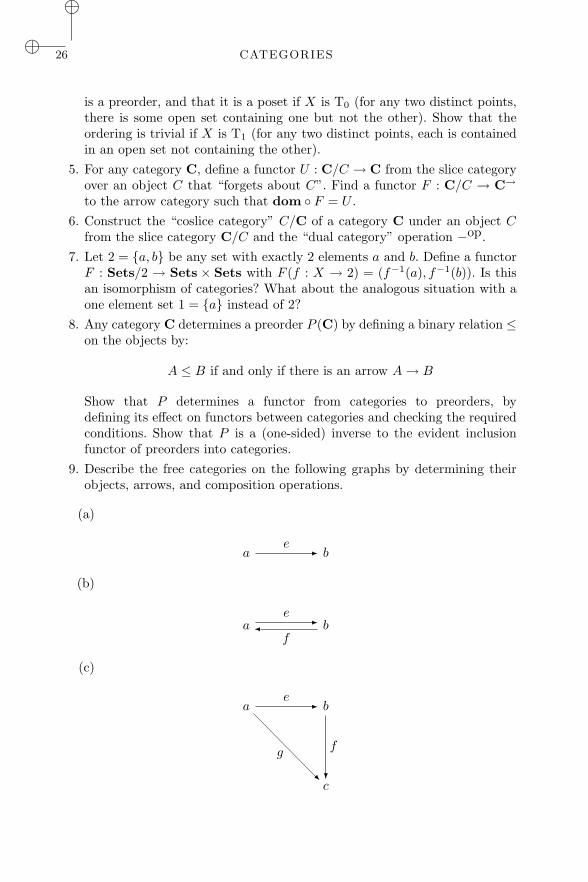
9. Describe the free categories on the following graphs by determining theirobjects, arrows, and composition operations.
(a)
ae - b
(b)
ae -�f
b
(c)
ae - b
c
f
?
g-
“chap01”2009/2/4page 27i
ii
i
ii
ii
EXERCISES 27
(d)
ae -�h
b d
c
f
?
g
�
10. How many free categories on graphs are there which have exactly six arrows?Draw the graphs that generate these categories.
11. Show that the free monoid functor
M : Sets→Mon
exists, in two different ways:
(a) Assume the particular choice M(X) = X∗ and define its effect
M(f) : M(A)→M(B)
on a function f : A→ B to be
M(f)(a1 . . . ak) = f(a1) . . . f(ak), a1, . . . ak ∈ A.
(b) Assume only the UMP of the free monoid and use it to determine M onfunctions, showing the result to be a functor.
Reflect on how these two approaches are related.12. Verify the UMP for free categories on graphs, defined as above with arrows
being sequences of edges. Specifically, let C(G) be the free category on thegraph G, so defined, and i : G→ U(C(G)) the graph homomorphism takingvertices and edges to themselves, regarded as objects and arrows in C(G).Show that for any category D and graph homomorphism f : G → U(D),there is a unique functor
h : C(G)→ D
with
U(h) ◦ i = h,
where U : Cat→ Graph is the underlying graph functor.13. Use the Cayley representation to show that every small category is
isomorphic to a “concrete” one, i.e. one in which the objects are sets andthe arrows are functions between them.
14. The notion of a category can also be defined with just one sort (arrows)rather than two (arrows and objects); the domains and codomains aretaken to be certain arrows that act as units under composition, which is
“chap01”2009/2/4page 28i
ii
i
ii
ii
28 CATEGORIES
partially defined. Read about this definition in section I.1 of Mac Lane’sCategories for the Working Mathematician, and do the exercise mentionedthere, showing that it is equivalent to the usual definition.