Catenaries and Suspension Bridges – The Shape of a Hanging String/Cable Tatsu Takeuchi * Department of Physics, Virginia Tech, Blacksburg VA 24061, USA (Dated: April 6, 2019) Demo presentation at the 2019 Spring Meeting of the Chesapeake Section of the American Asso- ciation of Physics Teachers (CSAAPT). FIG. 1. The Clifton Suspension Bridge in Bristol, UK. Opened in 1864. Photo by Gothick, Creative Commons Attribution- Share Alike 3.0 Unported license. I. INTRODUCTION We see suspension bridges all around the world and we all recognize the distinctive shape of the cables that support them. The question is, what is that shape? In these notes, I will derive what that shape is and introduce a simple demo that can be performed in class. I begin by discussing the shape of a catenary, namely, the shape of a hanging string/cable which is supporting its own weight. I will first use the variational method to derive the shape of the catenary, and then present a non-variational method which, naturally, leads to the same result. I will then apply the second method to the problem of suspension bridges and derive the shape of the suspension- bridge cable which is supporting the weight of the bridge hanging from it. Finally, I will discuss a simple demonstration that can be performed in class which compares the two results. * [email protected]
Transcript
Catenaries and Suspension Bridges – The Shape of a Hanging String/Cable
Tatsu Takeuchi∗
Department of Physics, Virginia Tech, Blacksburg VA 24061, USA(Dated: April 6, 2019)
Demo presentation at the 2019 Spring Meeting of the Chesapeake Section of the American Asso-ciation of Physics Teachers (CSAAPT).
FIG. 1. The Clifton Suspension Bridge in Bristol, UK. Opened in 1864. Photo by Gothick, Creative Commons Attribution-Share Alike 3.0 Unported license.
I. INTRODUCTION
We see suspension bridges all around the world and we all recognize the distinctive shape of the cables that supportthem. The question is, what is that shape? In these notes, I will derive what that shape is and introduce a simpledemo that can be performed in class.
I begin by discussing the shape of a catenary, namely, the shape of a hanging string/cable which is supporting its ownweight. I will first use the variational method to derive the shape of the catenary, and then present a non-variationalmethod which, naturally, leads to the same result.
I will then apply the second method to the problem of suspension bridges and derive the shape of the suspension-bridge cable which is supporting the weight of the bridge hanging from it.
Finally, I will discuss a simple demonstration that can be performed in class which compares the two results.
CSAAPT 2019 Spring Meeting Demo – Tatsu Takeuchi, Virginia Tech Department of Physics 2
II. REVIEW OF THE VARIATIONAL METHOD
The variational method is used to derive the Euler-Lagrange equations of motion from the action S, via theapplication of the principle of least action δS = 0 :
S =
∫ tB
tA
dtL(y, y) , y =dy
dt,
δS=0−−−→ ∂L
∂y− d
dt
∂L
∂y= 0 . (1)
However, it can be used in many other contexts as well. Whenever you need to minimize (or maximize) an integralof a functional F (y, y′) of a function y and its derivative y′, you obtain the Euler-Lagrange equation. To make sureeveryone is on board, I begin with a brief review of the formalism.
A. Minimization Problem
We would like to find the function y(x) which minimizes an integral of the form
P =
∫ b
a
dxF (y, y′) , y′ =dy
dx, (2)
under the condition that y(a) and y(b) are fixed. If we vary the function y(x) by a variation δy(x),
y(x) → y(x) + δy(x) , δy(a) = δy(b) = 0 , (3)
then the change in P will be
δP =
∫ b
a
dxF (y + δy, y′ + δy′)
=
∫ b
a
dx
{∂F
∂yδy +
∂F
∂y′δy′}
=
∫ b
a
dx
[∂F
∂yδy +
{d
dx
(∂F
∂y′δy
)−(d
dx
∂F
∂y′
)δy
}]=
∫ b
a
dx
{(∂F
∂y− d
dx
∂F
∂y′
)δy +
d
dx
(∂F
∂y′δy
)}=
∫ b
a
dx
{(∂F
∂y− d
dx
∂F
∂y′
)δy
}+
∫ b
a
dx
{d
dx
(∂F
∂y′δy
)}=
∫ b
a
dx
{(∂F
∂y− d
dx
∂F
∂y′
)δy
}+
[∂F
∂y′δy
]ba︸ ︷︷ ︸
= 0
=
∫ b
a
dx
{(∂F
∂y− d
dx
∂F
∂y′
)δy
}. (4)
In the penultimate line we have used δy(a) = δy(b) = 0. Therefore, for δP = 0 regardless of the choice of δy, we musthave
∂F
∂y− d
dx
∂F
∂y′= 0 . (5)
This is the Euler-Lagrange equation.
CSAAPT 2019 Spring Meeting Demo – Tatsu Takeuchi, Virginia Tech Department of Physics 3
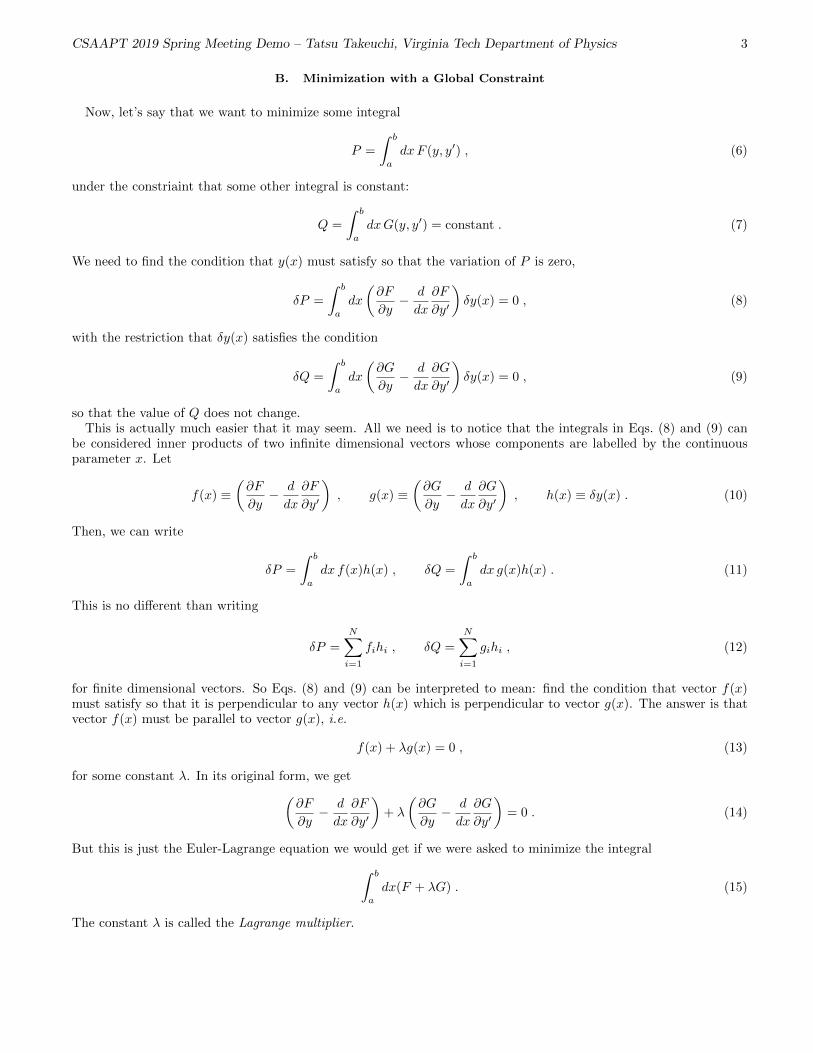
B. Minimization with a Global Constraint
Now, let’s say that we want to minimize some integral
P =
∫ b
a
dxF (y, y′) , (6)
under the constriaint that some other integral is constant:
Q =
∫ b
a
dxG(y, y′) = constant . (7)
We need to find the condition that y(x) must satisfy so that the variation of P is zero,
δP =
∫ b
a
dx
(∂F
∂y− d
dx
∂F
∂y′
)δy(x) = 0 , (8)
with the restriction that δy(x) satisfies the condition
δQ =
∫ b
a
dx
(∂G
∂y− d
dx
∂G
∂y′
)δy(x) = 0 , (9)
so that the value of Q does not change.This is actually much easier that it may seem. All we need is to notice that the integrals in Eqs. (8) and (9) can
be considered inner products of two infinite dimensional vectors whose components are labelled by the continuousparameter x. Let
f(x) ≡(∂F
∂y− d
dx
∂F
∂y′
), g(x) ≡
(∂G
∂y− d
dx
∂G
∂y′
), h(x) ≡ δy(x) . (10)
Then, we can write
δP =
∫ b
a
dx f(x)h(x) , δQ =
∫ b
a
dx g(x)h(x) . (11)
This is no different than writing
δP =
N∑i=1
fihi , δQ =
N∑i=1
gihi , (12)
for finite dimensional vectors. So Eqs. (8) and (9) can be interpreted to mean: find the condition that vector f(x)must satisfy so that it is perpendicular to any vector h(x) which is perpendicular to vector g(x). The answer is thatvector f(x) must be parallel to vector g(x), i.e.
f(x) + λg(x) = 0 , (13)
for some constant λ. In its original form, we get(∂F
∂y− d
dx
∂F
∂y′
)+ λ
(∂G
∂y− d
dx
∂G
∂y′
)= 0 . (14)
But this is just the Euler-Lagrange equation we would get if we were asked to minimize the integral∫ b
a
dx(F + λG) . (15)
The constant λ is called the Lagrange multiplier.
CSAAPT 2019 Spring Meeting Demo – Tatsu Takeuchi, Virginia Tech Department of Physics 4
III. SHAPE OF STRING SUSPENDED BETWEEN TWO POINTS
A. The Problem
Let’s figure out what the shape of a string of uniform linear mass density ρ will be when it is suspended betweentwo points A and B. The string will settle into a shape that minimizes the gravitational potential energy.
Take the x-axis in the horizontal direction and the y-axis in the vertical direction (up). If we describe the shapeof the string by specifying y as a function of x, y(x), then the potential energy of the string between points (x, y(x))and (x+ dx, y(x+ dx) = y + dy) will be
ρgy√dx2 + dy2 = ρgy
√1 + (y′)2 dx , (16)
where
y′ ≡ dy
dx. (17)
So the total potential energy will be
V = ρg
∫ b
a
y√
1 + (y′)2 dx , (18)
where a and b are the x-coordinates of the points A and B, respectively. We need to minimize this under the constraintthat the total length of the string does not change. The length of the string is given by the integral
` =
∫ b
a
√dx2 + dy2 =
∫ b
a
√1 + (y′)2 dx . (19)
This can be done using the Lagrange multiplier method discussed above.
B. The Solution
So to solve the string suspension problem, all we need to do is apply the Euler-Lagrange equation to the function
F = y√
1 + (y′)2 + λ√
1 + (y′)2 = (y + λ)√
1 + (y′)2 . (20)
(We have factored out the ρg for simplicity.) Since
∂F
∂y=√
1 + (y′)2 ,∂F
∂y′= (y + λ)
y′√1 + (y′)2
,
d
dx
∂F
∂y′=
(y′)2√1 + (y′)2
+ (y + λ)
(y′′√
1 + (y′)2− (y′)2y′′√
(1 + (y′)2)3
)=
(y′)2√1 + (y′)2
+ (y + λ)y′′√
1 + (y′)2
(1− (y′)2
1 + (y′)2
)=
(y′)2√1 + (y′)2
+ (y + λ)y′′√
(1 + (y′)2)3, (21)
we find
0 =∂F
∂x− d
dx
∂F
∂y′=√
1 + (y′)2 − (y′)2√1 + (y′)2
− (y + λ)y′′√
(1 + (y′)2)3
=1 + (y′)2√1 + (y′)2
− (y′)2√1 + (y′)2
− (y + λ)y′′√
(1 + (y′)2)3
=1√
1 + (y′)2− (y + λ)
y′′√(1 + (y′)2)3
=1√
1 + (y′)2
{1− (y + λ)
y′′
1 + (y′)2
}, (22)
or
0 = 1− (y + λ)y′′
1 + (y′)2. (23)
CSAAPT 2019 Spring Meeting Demo – Tatsu Takeuchi, Virginia Tech Department of Physics 5
Divide by (y + λ) and multiply by 2y′, then integrate:
We can drop the λ here by shifting the origin in the y direction. We get
k dx =k dy√k2y2 − 1
. (27)
Change variable to ξ = ky. Then
k dx =dξ√ξ2 − 1
, (28)
which can be integated to yield
kx = cosh−1 ξ = cosh−1 ky , (29)
or
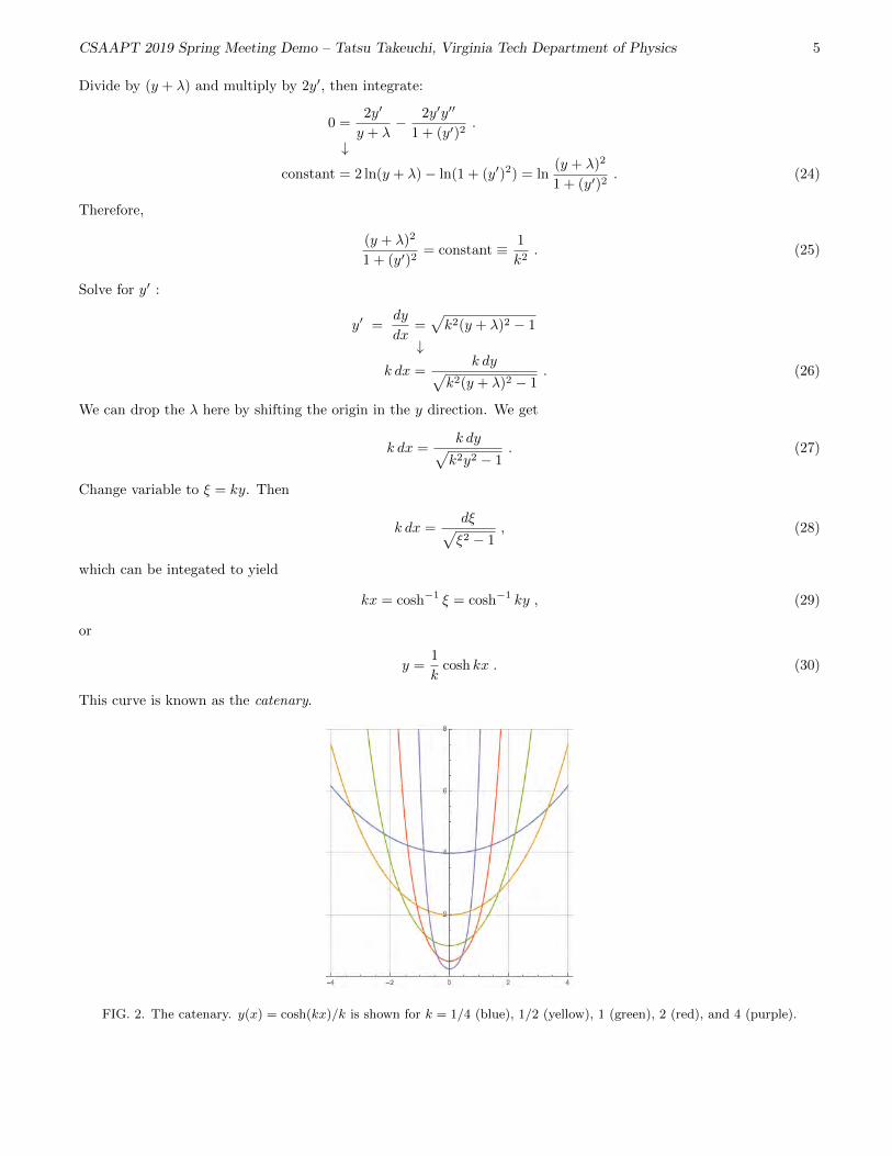
y =1
kcosh kx . (30)
This curve is known as the catenary.
FIG. 2. The catenary. y(x) = cosh(kx)/k is shown for k = 1/4 (blue), 1/2 (yellow), 1 (green), 2 (red), and 4 (purple).
CSAAPT 2019 Spring Meeting Demo – Tatsu Takeuchi, Virginia Tech Department of Physics 6
The parameter k is determined by the positions of the points A and B and the length of the string `. For the sakeof simplicity, let’s consider the case in which points A and B are at the same height and their horizontal separationis 2∆. We take the x-coordinate of point A to be −∆, and that of point B to be ∆. The length of the string betweenA and B will be given by
` =
∫ ∆
−∆
dx√
1 + (y′)2 . (31)
Since
y(x) =1
kcosh(kx)
↓y′(x) = sinh(kx) , (32)
we find
` =
∫ ∆
−∆
dx
√1 + sinh2(kx) =
∫ ∆
−∆
dx
√cosh2(kx) =
∫ ∆
−∆
dx cosh(kx)
=
[1
ksinh(kx)
]∆
−∆
=1
k
{sinh(k∆)− sinh(−k∆)
}=
2
ksinh(k∆) , (33)
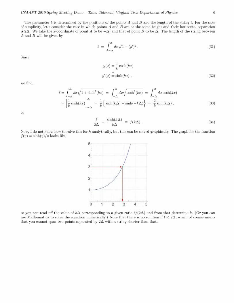
or
`
2∆=
sinh(k∆)
k∆≡ f(k∆) . (34)
Now, I do not know how to solve this for k analytically, but this can be solved graphically. The graph for the functionf(η) = sinh(η)/η looks like
so you can read off the value of k∆ corresponding to a given ratio `/(2∆) and from that determine k. (Or you canuse Mathematica to solve the equation numerically.) Note that there is no solution if ` < 2∆, which of course meansthat you cannot span two points separated by 2∆ with a string shorter than that.
CSAAPT 2019 Spring Meeting Demo – Tatsu Takeuchi, Virginia Tech Department of Physics 7
FIG. 3. Forces on a section of the suspended string.
IV. NON-VARIATIONAL APPROACH
A. The Catenary
The same result can be obtained via a non-variational method as follows. Choose your coordinate system so that(x, y) = (0, 0) is the lowest point of your suspended string. If the shape of the string is given by the function y(x),then y(0) = 0 and y′(0) = 0. Now, consider the forces acting on the part of the string between x = 0 and x = X.The length of the string between these points is
`X = `(0 < x < X) =
∫ X
0
√1 + (y′)2 dx , (35)
so the mass of that section is
mX = ρ `X = ρ
∫ X
0
√1 + (y′)2 dx , (36)
and the gravity acting on it
mXg = ρg`X = ρg
∫ X
0
√1 + (y′)2 dx . (37)
Denote the magnitude of the tension on the string at x = 0 by T0, and that at x = X by TX . T0 is pointinghorizontally left, while TX is pointing at an angle θ from the horizontal where tan θ = y′(X). Since the three forcesacting on the section under consideration must cancel, we must have
T0 = TX cos θ , mXg = TX sin θ , (38)
that is
y′(X) =TX sin θ
TX cos θ=
mXg
T0=
ρg
T0
∫ X
0
√1 + (y′)2 dx . (39)
Taking the derivative of both sides with respect to X, we obtain
y′′(X) =ρg
T0
√1 + {y′(X)}2 , (40)
or
y′′√1 + (y′)2
=ρg
T0≡ k . (41)
We suppress the arguments of the functions to simply the notation from this point on. Multiply both sides by y′ toobtain
y′y′′√1 + (y′)2
= ky′ . (42)
CSAAPT 2019 Spring Meeting Demo – Tatsu Takeuchi, Virginia Tech Department of Physics 8
Integrate: √1 + (y′)2 = ky + 1 , (43)
where we have chosen the integration constant so that y(0) = 0 implies y′(0) = 0. Solve for y′ and we find
y′ =√
(ky + 1)2 − 1 , (44)
or
y′√(ky + 1)2 − 1
= 1 , (45)
that is
kdy√(ky + 1)2 − 1
= kdx . (46)
Change variable to ξ = (ky + 1) to obtain
dξ√ξ2 − 1
= kdx . (47)
Solve:
cosh−1(ξ) = kx , (48)
that is:
ξ = ky + 1 = cosh(kx)↓
y =1
k
[cosh(kx)− 1
], (49)
and we see that we recover the same result as before. (The −1 inside the square brackets simply shifts the graphdownwards so that y(0) = 0.)
B. Suspension Bridge
FIG. 4. Forces on a section of a suspension bridge. We assume that the mass of the cable is negligible compared to that of thesuspended bridge section.
When a bridge is suspended from the cable (string) the shape will be slightly different. If we assume that the massof the cable is negligible compared to the mass of the bridge, and that the bridge has linear mass density µ, then themass supported by the cable between x = 0 and x = X will be given simply by
mX = µX , (50)
CSAAPT 2019 Spring Meeting Demo – Tatsu Takeuchi, Virginia Tech Department of Physics 9
and the gravity acting on it
mXg = µgX . (51)
Eq. (39) will be modified to
y′(X) =TX sin θ
TX cos θ=
mXg
T0=
µg
T0X . (52)
This can be trivially integrated to yield
y(X) =µg
2T0X2 , (53)
or setting µg/T0 ≡ K, and rewriting X as x, we obtain
y =K
2x2 . (54)
The constant K must again be determined from the condition that the length of the string is fixed. This time,
y′ = Kx , (55)
and we have
` =
∫ ∆
−∆
dx√
1 + (y′)2 =
∫ ∆
−∆
dx√
1 + (Kx)2 , (56)
or
K` =
∫ K∆
−K∆
dξ√
1 + ξ2 , ξ ≡ Kx . (57)
Change variable: ξ = sinh(ζ), dξ = dζ cosh(ζ). Then
K` =
∫ sinh−1(K∆)
− sinh−1(K∆)
dζ cosh2 ζ =
∫ sinh−1(K∆)
− sinh−1(K∆)
dζ1 + cosh 2ζ
2
=
[ζ
2+
sinh 2ζ
4
]sinh−1(K∆)
− sinh−1(K∆)
= sinh−1(K∆) +
[sinh ζ cosh ζ
2
]sinh−1(K∆)
− sinh−1(K∆)
= sinh−1(K∆) +K∆√
1 + (K∆)2 , (58)
or
`
2∆=
sinh−1(K∆)
2K∆+
1
2
√1 + (K∆)2 ≡ g(K∆) . (59)
Again, I do not know how to write ∆ as an analytic function of `/(2∆) so we use a graphical method (or Mathematica).
The graph of g(η) = sinh−1(η)/(2η) +√
1 + η2/2 looks like:
from which we can read off the value of K∆ when given `/(2∆), from which we can determine K.
CSAAPT 2019 Spring Meeting Demo – Tatsu Takeuchi, Virginia Tech Department of Physics 10
C. Catenary ↔ Suspension Bridge Comparison
The difference it the shapes of catenaries and suspension-bridge-cables (parabolas) are shown below in FIG. 5. Theseven cases shown are for
As is evident from the graph, the difference in hardly noticeable for small `/(2∆). The shapes of actual suspension-bridge cables fall somewhere in between the two cases since they support both their own weight and the weight ofthe bridge. The small difference is important for the engineers who are constructing the bridge, but it is impossibleto tell the difference from photographs taken from afar.
FIG. 5. Comparison of the shapes of catenaries (blue) and suspension-bridge-cables (parabolas, yellow). The cases shown arefrom top to bottom `/(2∆) = 1.1, 1.2, 1.3, 1.4, 1.5, 2, and 3.
CSAAPT 2019 Spring Meeting Demo – Tatsu Takeuchi, Virginia Tech Department of Physics 11
V. THE DEMOS
A. Catenary
Plot a graph of the hyperbolic cosine function using Mathematica (or Desmos, or some other program) and projectit onto a screen. Hold a piece of string against it and demonstrate that it does indeed fall into the shape of a catenary.
B. Suspension Bridge
Use Mathematica to overlay a graph of a parabola onto a photo of a suspension bridge. You can “Insert” the photointo Mathematica as a “Picture” and the use the “Overlay” command to superpose a graph onto it.
Graph overlaid over photo by Gothick, Creative Commons Attribution-Share Alike 3.0 Unported license.
Graph overlaid over photo by:Author: D Ramey LoganGolden Gate Bridge Dec 15 2015 by D Ramey Logan.jpg from Wikimedia CommonsLicense: Creative Commons Attribution 4.0
CSAAPT 2019 Spring Meeting Demo – Tatsu Takeuchi, Virginia Tech Department of Physics 12
C. Catenary and Suspension Bridge Comparison
To be able to tell the difference between a catenary and a parabola, we need `/(2∆) to be large. So let’s use`/(2∆) = 3. We will prepare a piece of string 6 feet long and suspend it between two points that are 2 feet apart. Ifwe attach weights to it so that they are equally spaced horizontally when the string is in the shape of a parabola, wecan simulate a horizontal bridge of uniform mass density hanging from it.
Things to prepare
1. 6’-and-a-few-inches length piece of light string ×2.
2. 19 fishing weights.
On one of the strings, attach the fishing weights at the following locations from the center:
1. 0 inches (center)
2. 1.26 inches (3.2 cm, both sides)
3. 2.82 inches (7.2 cm, both sides)
4. 4.85 inches (12.3 cm, both sides)
5. 7.45 inches (18.9 cm, both sides)
6. 10.6 inches (27.0 cm, both sides)
7. 14.4 inches (36.7 cm, both sides)
8. 18.9 inches (47.9 cm, both sides)
9. 23.9 inches (60.8 cm, both sides)
10. 29.6 inches (75.3 cm, both sides)
11. 36.0 inches (91.4 cm. No weights here. Just mark the spots since this is where you need to hold the string.)
Project FIG. 5 onto a screen and adjust the magnification so that the points where the strings are suspended fromare separated by two feet. Hold the strings with and without the weights against the screen and compare the shapeswith the graphs.
How to determine where to place the weights:
For different values of ` and ∆, the locations of the weights can be determined using the function g(η) we definedin Eq. (59), namely:
g(η) =sinh−1(η)
2η+
√1 + η2
2. (61)
If we want to simulate the vertical cables of the suspension bridge being at