Causal Inference by Quantile Regression Kink Designs

Harold D. Chiang∗ Yuya Sasaki†‡

Johns Hopkins University

August 30, 2016

Abstract

The quantile regression kink design (QRKD) is proposed by empirical researchers as a potential

method to assess heterogeneous treatment effects under suitable research designs, but its causal

interpretation remains unknown. We propose causal interpretations of the QRKD estimand. Under

flexible heterogeneity and endogeneity, the sharp and fuzzy QRKD estimands measure weighted

averages of heterogeneous marginal effects at respective conditional quantiles of outcome given a

designed kink point. In addition, we develop weak convergence results for the QRKD estimator

as a local quantile process for the purpose of conducting statistical inference of heterogeneous

treatment effects using the QRKD. Applying our methods to the Continuous Wage and Benefit

History Project (CWBH) data, we find significantly heterogeneous positive moral hazard effects

of unemployment insurance benefits on unemployment durations in Louisiana between 1981 and

1982. We find that these effects are larger for individuals with longer unemployment durations.

Keywords: causal inference, heterogeneous treatment effects, identification, regression kink design,

quantile regression, unemployment duration.

∗hchiang7@jhu.edu. Department of Economics, Johns Hopkins University.†sasaki@jhu.edu. Department of Economics, Johns Hopkins University.‡We would like to thank Patty Anderson and Bruce Meyer for kindly agreeing to our use of the CWBH data. We ben-

efited from very useful comments by Andrew Chesher, Antonio Galvao, Emmanuel Guerre, Blaise Melly, Jungmo Yoon,

seminar participants at Academia Sinica, National Chengchi University, National University of Singapore, Otaru Uni-

versity of Commerce, Penn State University, Queen Mary University of London, University of Pittsburgh and University

of Surrey, and conference participants at AMES 2016, CeMMAP-SNU-Tokyo Conference on Advances in Microecono-

metrics, ESEM 2016, New York Camp Econometrics XI. All remaining errors are ours.

1

1 Introduction

Some recent empirical research papers, including Nielsen, Sørensen and Taber (2010), Landais (2015),

Simonsen, Skipper and Skipper (2015), Card, Lee, Pei and Weber (2016), and Dong (2016), conduct

causal inference via the regression kink design (RKD). A natural extension of the RKD with a flavor

of unobserved heterogeneity is the quantile RKD (QRKD), which is the object that we explore in this

paper. Specifically, consider the quantile derivative Wald ratio of the form

QRKD(τ) =limx↓x0

∂∂xQY |X(τ | x)− limx↑x0

∂∂xQY |X(τ | x)

limx↓x0ddxb(x)− limx↑x0

ddxb(x)

(1.1)

at a design point x0 of a running variable x, where QY |X(τ |x) := inf{y : F (y|x) ≥ τ} denotes the τ -th

conditional quantile function of Y given X = x, and b is a policy function. Note that it is analogous

to the RKD estimand of Card, Lee, Pei and Weber (2016):

RKD =limx↓x0

∂∂x E[Y | X = x]− limx↑x0

∂∂x E[Y | X = x]

limx↓x0ddxb(x)− limx↑x0

ddxb(x)

, (1.2)

except that the conditional expectations in the numerator are replaced by the corresponding condi-

tional quantiles. While the QRKD estimand (1.1) is of potential interest in the empirical literature for

assessment of heterogeneous treatment effects (e.g., Landais (2011) considers (1.1)), little seems known

about theories of identification, estimation, and inference. This paper develops causal interpretation

(identification) and estimation theories for the QRKD estimand (1.1). Consequently, we also propose

methods of inference for heterogeneous treatment effects based on the QRKD.

Causal analysis for types of estimands in the Wald-ratio form, like (1.1) and (1.2), dates back to the

seminal paper by Imbens and Angrist (1994). Making causal interpretations of the QRKD estimand

(1.1) is perhaps more challenging than the mean RKD estimand (1.2) because the differentiation

operator ddx and the conditional quantile do not ‘swap.’ For the mean RKD estimand (1.2), the

interchangeability of the differentiation operator and the expectation (integration) operator allows

each term of the numerator in (1.2) to be additively decomposed into two parts, namely the causal

effects and the endogeneity effects. Taking the difference of two terms in the numerator then cancels out

2

the endogeneity effects, leaving only the causal effects. This trick allows the mean RKD estimand (1.2)

to have causal interpretations in the presence of endogeneity. Due to the lack of such interchangeability

for the case of quatiles, this trick is not straightforwardly inherited by the quantile counterpart (1.1).

Having said this, we show in Section 2.1 and more formally in Section 2.2 that a similar decomposition

is possible for the QRKD estimand (1.1), and therefore argue that its causal interpretations are possible

even under the lack of monotonicity. Specifically, we show that the QRKD estimand corresponds to

the quantile marginal effect under monotonicity and to a weighted average of marginal effects under

non-monotonicity and/or with fuzzy design in a similar manner to Card, Lee, Pei and Weber (2016).

For estimation of the causal effects, we propose a sample-counterpart estimator for the QRKD

estimand (1.1) in Sections 3. To derive its asymptotic properties, we take advantage of the existing

literature on uniform Bahadur representations for quantile-type loss functions, including Kong, Linton

and Xia (2010), Guerre and Sabbah (2012), Sabbah (2014), and Qu and Yoon (2015a). Qu and Yoon

(2015b) apply the results of Qu and Yoon (2015a) to develop methods of statistical inference with

quantile regression discontinuity designs (QRDD), which are closely related to our QRKD framework.

We take a similar approach with suitable modifications to derive asymptotic properties of our QRKD

estimator. Weak convergence results for the estimator as a quantile process are derived. Applying

the weak convergence results, we propose procedures for testing treatment significance and treatment

heterogeneity following Koenker and Xiao (2002), Chernozhukov and Fernandez-Val (2005) and Qu

and Yoon (2015b). Simulation studies presented in Section 4 support the theoretical properties.

Literature: The method studied in this paper falls in the broad framework of design-based causal

inference, including RDD and RKD. There is an extensive body of literature on RDD by now –

see for example the special issue of Journal of Econometrics edited by Imbens and Lemieux (2008)

and the literature reviews by Imbens and Wooldridge (2009; Sec. 6.4) and Lee and Lemieux (2010).

The first extension to quantile treatment effects in the RDD framework was made by Frandsen,

Frolich and Melly (2012). More recently, Qu and Yoon (2015b) develop uniform inference methods

3

with QRDD that empirical researchers can use to test a variety of important empirical questions on

heterogeneous treatment effects. While the RDD has a rich set of empirical and theoretical results

including the quantile extensions, the RKD method which developed more recently does not have a

quantile counterpart in the literature yet, despite potential demands for it by empirical researchers

(e.g., Landais, 2011). Our paper can be seen as either a quantile extension to Card, Lee, Pei and

Weber (2016) or a RKD counterpart of Frandsen, Frolich and Melly (2012) and Qu and Yoon (2015b).

2 Causal Interpretation of the QRKD Estimand

In this section, we develop some causal interpretations of the QRKD estimand (1.1). For the purpose

of illustration, we first present a simple case with rank invariance in Section 2.1. It is followed by a

formal argument for general cases in Section 2.2.

2.1 Illustration: Causal Interpretation under Rank Invariance

The causal relation of interest is represented by the structural equation

y = g(b, x, ε).

The outcome y is determined through the structural function g by two observed factors, b ∈ R and

x ∈ R, and a scalar unobserved factor, ε ∈ R. We assume that g is monotone increasing in ε, effectively

imposing the rank invariance; causal interpretations in a more general setup with non-monotone g

and/or multivariate ε is established in Section 2.2. The factor b is a treatment input, and is in turn

determined by the running variable x through the structural equation

b = b(x)

for a known policy function b. We say that b has a kink at x0 if b′(x+0 ) := limx→x+0

db(x)dx 6=

limx→x−0db(x)dx =: b′(x−0 ) is true, where x → x+

0 and x → x−0 mean x ↓ x0 and x ↑ x0, respectively.

4

Throughout this paper, we assume that the location, x0, of the kink is known from a policy-based

research design, as is the case with Card, Lee, Pei and Weber (2016).

Assumption 1. b′(x+0 ) 6= b′(x−0 ) holds, and b is continuous on R and differentiable on R \ {x0}.

The structural partial effects are g1(b, x, ε) := ∂∂bg(b, x, ε), g2(b, x, ε) := ∂

∂xg(b, x, ε) and g3(b, x, ε) :=

∂∂εg(b, x, ε). In particular, a researcher is interested in g1 which measures heterogeneous partial effects

of the treatment intensity b on an outcome y. While the structural partial effect g1 is of interest, it

is not clear if the QRKD estimand (1.1) provides any information about g1. In this section, we argue

that (1.1) does have a causal interpretation in the sense that it measures the structural causal effect

g1(b(x0), x0, ε) at the τ -th conditional quantile of ε given X = x0.

Under regularity conditions (to be discussed in Section 2.2 in detail), some calculations yield the

decomposition

∂

∂xQY |X(τ | x) = g1(b(x), x, ε) · b′(x) + g2(b(x), x, ε)−

∫ ε−∞

∂∂xfε|X(e | x)de

fε|X(ε | x)· g3(b(x), x, ε), (2.1)

where τ = Fε|X(ε | x). The first term on the right-hand side is the partial effect of the running variable

x on the outcome y through the policy function b. The second term is the direct partial effect of the

running variable on the outcome y. The third term measures the effect of endogeneity in the running

variable x. We can see that this third term is zero under exogeneity, ∂∂xfε|X = 0. In order to get the

causal effect g1(b(x), x, ε) of interest through the QRKD estimand (1.1), therefore, we want to remove

the last two terms in (2.1).

Suppose that the designed kink condition of Assumption 1 is true, but all the other functions, g1,

g2, g3, 1/fε|X and ∂∂xfε|X , in the right-hand side of (2.1) are continuous in (b, x) at (b(x0), x0). Then,

(2.1) yields

∂∂xQY |X(τ | x+

0 )− ∂∂xQY |X(τ | x−0 )

b′(x+0 )− b′(x−0 )

= g1(b(x0), x0, ε),

showing that the QRKD estimand (1.1) measures the structural causal effect g1(b(x0), x0, ε) of b on

y for the subpopulation of individuals at the τ -th conditional quantile of ε given X = x0. This

5

section provides only an informal argument for ease of exposition, but Section 2.2 provides a formal

mathematical argument under a general setup without the rank invariance assumption. Furthermore,

we provide a result for the case of fuzzy QRKD in Section A.1 in the supplementary appendix.

2.2 General Result: Causal Interpretation without Rank Invariance

In this section, we continue to use the basic settings from Section 2.1 except that the unobserved

factors ε are now allowed to be M -dimensional, as opposed to be a scalar. As such, we can consider

general structural functions g without the rank invariance. Define the lower contour set of ε evaluated

by g(b(x), x, ·) below a given level of y as follows:

V (y, x) = {ε ∈ RM |g(b(x), x, ε) ≤ y}.

Its boundary is denoted by ∂V (y, x). Furthermore, the velocities of the boundary ∂V (y, x) at u

with respect to a change in y and a change in x are denoted by ∂υ(y, x;u)/∂y and ∂υ(y, x;u)/∂x,

respectively. Σ denotes an (M − 1)-dimensional rectangle. For a short hand notation, we write

h(x, ε) = g(b(x), x, ε) and h1(x, ε) = ∂h(x,ε)∂x . Let mM and HM−1 denote the Lebesgue measure on RM

and the Hausdorff measure on ∂V (y, x), respectively.1 Letting X = supp(X), we make the following

assumptions.

Assumption 2. (i) h(·, ε) is continuously differentiable on X \ {x0} for all ε ∈ E and h(x, ·) is

continuously differentiable for all x ∈ X . (ii) ‖∇εh(x, ·)‖ 6= 0 on ∂V (y, x) for all (x, y) ∈ X × Y.

(iii) The conditional distribution of ε given X is absolutely continuous with respect to mM , fε|X is

continuously differentiable, and fε|X ∈ C1(X ;L1(RM )) is true. (iv)∫∂V (y,x) fε|X(ε | x)dHM−1(ε) > 0

for all (x, y) ∈ X ×Y. (v) ∂V (y, ·) ∈ C1(Σ×X ;RM ) holds for all y ∈ Y and ∂V (·, x) ∈ C1(Σ×Y;RM )

holds for all x ∈ X . (vi) ∂υ(y, · ; ·)/∂x ∈ C1(X ;L1(Σ)) holds for all y ∈ Y and ∂υ(·, x ; ·)/∂y ∈1We obtain the (M − 1)-dimensional Hausdorff measure by the restriction of the function HM−1 : 2RM

→ R defined

by HM−1(S) = supδ>0 inf{∑∞

i=1(diamUi)M−1 | ∪∞i=1Si ⊃ S, diamSi < δ

}to the collection of Caratheodory-measurable

sets.

6

C1(Y;L1(Σ)) holds for all x ∈ X .

Assumption 3. Let γ(x, ε) := ‖∇εh(x, ε)‖−1. There exist values p > 1 and q > 1 satisfying p−1 +

q−1 = 1 such that ‖γ(x, · )‖Lp(∂V (y,x),HM−1) < ∞ and ‖fε‖Lq(∂V (y,x),HM−1) < ∞ hold for all (x, y) ∈

X × Y.

Assumption 4. There exists a function w ∈ L1(∂V (y, x), HM−1) such that

|γ(x, ε)hx(x, ε)fε|X(ε|x)| ≤ w(ε) for all ε ∈ ×V (y, x) for all x ∈ X .

Assumption 5. limx→x+0∂∂xQY |X(τ |x) and limx→x−0

∂∂xQY |X(τ |x) exist.

Assumptions 2 and 3 are used to derive a structural decomposition of the quantile partial deriva-

tive – see Sasaki (2015) for detailed discussions of these assumptions. The regularity conditions in

Assumptions 4 and 5 together facilitate the dominated convergence theorem to make a structural sense

of the QRKD estimand (1.1). With B(y, x) denoting the collection of Borel subsets of ∂V (y, x), we

define the function µy,x : B(y, x)→ R by

µy,x(S) :=

∫s

1‖∇εh(x,ε)‖fε|X(ε|x)dHM−1(ε)∫

∂V (y,x)1

‖∇εh(x,ε)‖fε|X(ε|x)dHM−1(ε)for all S ∈ B(y, x).

The next theorem claims that this is a probability measure and gives weights with respect to which

the QRKD estimand (1.1) measures the average structural causal effect of the treatment intensity b

on an outcome y for those individuals at the τ -th conditional quantile of Y given X = x0.

Theorem 1. Suppose that Assumptions 1, 2, 3, 4 and 5 hold. Then, µy,x is a probability measure on

∂V (y, x) for all (x, y) ∈ X × Y, and we have

QRKD(τ) =

∫g1(b(x0), x0, ε)dµy,x0(ε) = Eµy,x0 [g1(b(x0), x0, ε)] (2.2)

where τ = FY |X(y | x0).

A proof is provided below at the end of the current section. We may derive a similar causal inter-

pretation for the case of fuzzy QRKD – see Section A.1 in the supplementary appendix. As is often the

7

case in the treatment literature (e.g., Angrist and Imbens, 1995), this theorem shows a causal interpre-

tation in terms of a weighted average. Specifically, (2.2) shows that the QRKD estimand (1.1) measures

a weighted average of the heterogeneious causal effects g1(b(x0), x0, ε) displayed on the right-hand side

of (2.2). The weights given in the definition of µy,x0 are proportional to fε|X(ε|x0)/‖∇εh(x0, ε)‖ which

is positive on the conditional support of ε given X = x0. In other words, the QRKD estimand mea-

sures a strict convex combination of the ceteris paribus causal effects of b on y for those individuals

at the τ -th conditional quantile of Y given X = x0. One may worry about the obscurity of the causal

interpretations under the ‘weighted’ averages. There are two special cases where the QRKD estimand

allows for causal interpretations in terms of purely unweighted averages, i.e., ‖∇εh(x0, ε)‖ is constant

in ε. One example is the case where the structural function g(b, x, · ) is monotone in a scalar unob-

servable ε, which is the special case discussed in Section 2.1. The other example is the more general

case where the structure exhibits partial additivity, e.g., g(b, x, ε) =∑M

m=1 εmgm(b, x). When an em-

pirical practitioner is reluctant to make either of these assumptions, the QRKD estimand can be still

interpreted as a weighted average measurement of the treatment effects among the subpopulation of

individuals at the τ -th conditional quantile of Y given X = x0. In either of these cases, heterogeneity

in values of the QRKD estimand across quantiles τ can be used as evidence for heterogeneity in treat-

ment effects. Therefore, we can still conduct statistical inference for heterogeneous treatment effects

based on the weak convergence results obtained in Section 3 and Section B.5 in the supplementary

appendix.

Proof of Theorem 1: The first result that µy,x is a probability measure on ∂V (y, x) follows

from Lemma 2 of Sasaki (2015) under Assumption 3. Next, by Lemma 1 of Sasaki (2015) under

Assumptions 2 and 3, the QPD ∂∂xQY |X(τ | x) exists and

∂

∂xQY |X(τ | x) =

∫∂V (y,x)

hx(x,ε)‖∇εh(x,ε)‖

fε|X(ε|x)·Mπ(M−1)/2

2M−1Γ(M+12

)dHM−1(ε)−

∫V (y,x)

∂∂xfε|X(ε | x)dmM (ε)∫

∂V (y,x)1

‖∇εh(x,ε)‖fε|X(ε|x)·Mπ(M−1)/2

2M−1Γ(M+12

)dHM−1(ε)

= Eµy,x [hx(x, ε)]−A(y, x),

8

where Γ is the Gamma function and A is defined by

A(y, x) :=

∫V (y,x)

∂∂xfε|X(ε | x)dmM (ε)∫

∂V (y,x)1

‖∇εh(x,ε)‖fε|X(ε|x)·Mπ(M−1)/2

2M−1Γ(M+12

)dHM−1(ε)

Note that g2 = ∂g∂x is continuous in x by Assumption 2 (i). Also, µy,x(ε) is continuous in x for each

fixed y according to parts (i), (ii) and (iii) of Assumption 2. Furthermore, Assumption 2 (i), (ii), (iii)

and (iv) imply that A(y, x) is well-defined and is continuous in x for all y ∈ Y. Therefore, applying

the dominated convergence theorem under Assumptions 4 and 5 yields

limx→x+0

∂

∂xQY |X(τ | x) = lim

x→x+0

∫{hx(x, ε)}dµy,x(ε)− lim

x→x+0A(y, x)

=

∫limx→x+0

∂

∂x{g(b(x), x, ε)}dµy,x(ε)−A(y, x0)

=

∫limx→x+0

{g1(b(x), x, ε)b′(x) + g2(b(x), x, ε)}dµy,x(ε)−A(y, x0)

=

∫{g1(b(x0), x0, ε)b

′(x+0 ) + g2(b(x0), x0, ε)}dµy,x0(ε)−A(y, x0)

Similarly, taking the limit from the left, we have

limx→x−0

∂

∂xQY |X(τ | x) =

∫{g1(b(x0), x0, ε)b

′(x−0 ) + g2(b(x0), x0, ε)}dµy,x0(ε)−A(y, x0).

Taking the difference of the right and left limits eliminates∫g2(b(x0), x0, ε)dµy,x0(ε) − A(y, x0), and

thus produces

limx→x+0

∂

∂xQY |X(τ | x)− lim

x→x−0

∂

∂xQY |X(τ | x) = [b′(x+

0 )− b′(x−0 )]Eµy,x0 [g1(b(x0), x0, ε)] .

Finally, note that Assumption 1 has b′(x+0 ) − b′(x−0 ) 6= 0, and hence we can divide both sides of the

above equality by b′(x+0 )− b′(x−0 ). This gives the desired result.

3 Estimation and Inference

3.1 The Estimator and Its Asymptotic Distribution

We propose to estimate the QRKD estimand (1.1) by the sample counterpart

QRKD(τ) =β+(τ)− β−(τ)

limx↓x0 b′(x)− limx↑x0 b

′(x)(3.1)

9

with the two terms in the numerator given by the one-sided local linear quantile smoothers

β+(τ) = ι′2 arg minα,β

n∑i=1

d+i K(

xi − x0

hn,τ)ρτ (yi − α− β(xi − x0)) and

β−(τ) = ι′2 arg minα,β

n∑i=1

d−i K(xi − x0

hn,τ)ρτ (yi − α− β(xi − x0)),

for τ ∈ T , where T ⊂ (0, 1) is a closed interval, K is a kernel function, ρτ (u) = u(τ − 1{u < 0}),

d+i = 1{xi ≥ x0}, d−i = 1{xi ≤ x0}, and ι2 = [0, 1]′. A researcher observing a sample {yi, xi}ni=1 of n

observations can compute (3.1) explicitly to estimate (1.1). In the remainder of this section, weak con-

vergence results are developed for the quantile processes of β+(τ) and β−(τ), which in turn yield weak

convergence results for the quantile process of the QRKD estimator of treatment effects. Furthremore,

using the weak convergence results, we propose some tests of hypotheses concerning heterogeneous

treatment effects. With the kernel-dependent constant matrices N+(τ) =∫∞

0 (1, u)′(1, u)K(u)du and

N−(τ) =∫ 0−∞(1, u)′(1, u)K(u)du, we make the following assumptions.

Assumption 6. There exist x > x0 and x < x0 such that the following conditions are satisfied:

(i) (a) The density function fX(·) exists and is continuously differentiable in a neighborhood of x0 and

0 < fX(x0) <∞. (b) {(yi, xi)}ni=1 is an i.i.d. sample of n observations of the bivariate random vector

(Y,X).

(ii) (a) fY |X(y|x) is Lipschitz continuous on [inf(τ,x)∈T×(x0,x]Q(τ |x), sup(τ,x)∈T×(x0,x]Q(τ |x)]×(x0, x]

and [inf(τ,x)∈T×[x,x0)Q(τ |x), sup(τ,x)∈T×[x,x0)Q(τ |x)]× [x, x0). (b) There exist finite constants fL > 0,

fU > 0 and ε > 0, such that fY |X(Q(τ |x) + η|x) lies between fL and fU for all τ ∈ T , |η| ≤ ε and

x ∈ [x, x].

(iii) (a) Q(τ |x+0 ), ∂Q(τ |x+

0 )/∂τ ,Q(τ |x−0 ), and ∂Q(τ |x−0 )/∂τ exist and are Lipschitz continuous in τ on

T . (b) ∂Q(τ |x)/∂x and ∂Q2(τ |x)/∂x2 exist and are Lipschitz continuous on {(x, τ)|x ∈ (x0, x], τ ∈ T}

and {(x, τ)|x ∈ [x, x0), τ ∈ T}.

(iv) The kernel K is compactly supported, Lipschitz, differentiable, and satisfying K(·) ≥ 0,∫K(u)du =

1,∫uK(u)du = 0. Also,

∫∞0 ukK(u)du and

∫ 0−∞ u

kK(u)du are finite for k = 1, 2, 3. The matrices

10

N+ and N− are positive definite.

(v) The bandwidths satisfy hn,τ = c(τ)hn, where nh3n →∞ and hn = o(n−1/5) as n→∞, and c(·) is

Lipschitz continuous satisfying 0 < c ≤ c(τ) ≤ c <∞ for all τ ∈ T.

Part (i) (a) requires smoothness of the density of the running variable. This can be interpreted as

the design requirement for absence of endogenous sorting across the kink point x0. The i.i.d assumption

in part (i) (b) is usually considered to be satisfied for micro data of random samples. Part (ii) concerns

about regularities of the conditional density function of Y given X. It requires sufficient smoothness,

but does not rule out quantile regression kinks at x0, which is the main crucial assumption for our

identification argument. Part (iii) concerns about regularities of the conditional quantile function of

Y given X. Like part (ii), it does not rule out quantile regression kinks at x0. Part (iv) prescribes

requirements for kernel functions to be chosen by users. In Section 4 for simulation studies, we propose

an example of such a choice to satisfy this requirement. Finally, part (v) specifies the rate at which

the bandwidth parameters diminish as the sample size becomes large. It obeys the standard rate for

a first-order derivative estimation, but we also require its uniformity over quantiles τ in T . While

hn = o(n−1/5) is required for a valid inference without bias reduction, this requirement can be relaxed

to hn = O(n−1/5) if one is willing to make additional assumptions and to take an additional step

of bias reduction – see Section B.5 in the supplementary appendix. Under this set of assumptions,

we obtain uniform Bahadur representations for the component estimators, β+(τ) and β−(τ), of our

interest – see Lemma 3 in Section B.2 in the supplementary appendix.

Applying Lemma 3, we now establish weak convergence results for our component estimators, β+

and β−. We focus on β+, but a similar result follows for β−.

Theorem 2. Under Assumptions 6, we have the weak convergence

√nh3

n,τfX(x0)fY |X(Q(τ |x+0 )|x+

0 )×(β+(τ)− ∂Q(τ |x+

0 )

∂x− hn,τ

ι′2(N+)−1

2

∫ ∞0

u2∂2Q(τ |x+

0 )

∂x2(1, u)′K(u)du

)⇒ G+(τ),

11

for the zero mean Gaussian process G+(τ) defined over T with covariance function

E(G+(r)G+(s)) = (κ(r)κ(s))−1/2(r ∧ s− rs)ι′2(N+)−1T+(r, s)(N+)−1ι2,

for each r, s ∈ T , where T+(r, s) =∫∞

0

[1 u

κ(r)

]′K( u

κ(r))

[1 u

κ(s)

]K( u

κ(s))du with κ(τ) = hn,τ/hn,1/2 =

c(τ)c(1/2) ≥ (c/c) > 0. A similar result follows for β−(τ).

A proof is provided in Section B.3 in the supplementary appendix. While we write the above weak

convergence result explicitly accounting for the finite-sample bias term hn,τι′2(N+)−1

2

∫∞0 u2 ∂

2Q(τ |x+0 )

∂x2(1, u)′

K(u)du, it goes away in large sample as hn,τ goes to zero uniformly in τ ∈ T . In other words, this

bias term can be considered to be absent in the above equation. With this said, in case one wish to

reduce this finite-sample bias at the cost of additional assumptions, we propose in Section B.5 in the

supplementary appendix how to estimate this bias term.

We are now ready to present a weak convergence result for our QRKD estimator (3.1). By Section

2.1 of Gine and Nickl (2015), the sum of two independent Gaussian processes is a Gaussian process

with the mean (respectively, the covariance) being the sum of the means (respectively, the covariances).

Corollary 1. Under Assumptions 1 and 6 we have the weak convergence

√nh3

n,τ

(QRKD(τ)−QRKD(τ)

)⇒Y (τ) =

1√fX(x0)

(b′(x+

0 )− b′(x−0 ))[ G+(τ)

fY |X(Q(τ |x+0 )|x+

0 )− G−(τ)

fY |X(Q(τ |x−0 )|x−0 )

].

The random process Y (·) has mean zero, as G+(τ) and G−(τ) do. For any pair r, s ∈ T of

quantiles, the covariance can be computed by:

E[Y (r)Y (s)] =1

fX(x0)(b′(x+0 )− b′(x−0 ))2

×[

EG+(r)G+(s)

fY |X(Q(r|x+0 )|x+

0 )fY |X(Q(s|x+0 )|x+

0 )+

EG−(r)G−(s)

fY |X(Q(r|x−0 )|x−0 )fY |X(Q(s|x−0 )|x−0 )

].

This uniform convergence result is applicable to many purposes, such as to compute uniform confidence

bands for the QRKD. Of particular interest may be the empirical tests discussed in Section 3.2.

12

3.2 Testing for Heterogeneous Treatment Effects

Researchers are often interested in the following hypotheses regarding heterogeneous treatment effects.

Treatment Significance HS0 : QRKD(τ) = 0 for all τ ∈ T.

Treatment Heterogeneity HH0 : QRKD(τ) = QRKD(τ ′) for all τ, τ ′ ∈ T.

They are both considered in Koenker and Xiao (2002), Chernozhukov and Fernandez-Val (2005) and

Qu and Yoon (2015b), among others. Following the approach of these preceding papers, the two

hypotheses, HS0 and HH

0 , may be tested using the statistics

WSn(T ) =√nh3

n,τ supτ∈T|QRKD(τ)| and

WHn(T ) =√nh3

n,τ supτ∈T

∣∣∣∣QRKD(τ)−∫TQRKD(τ ′)dτ ′

∣∣∣∣,respectively. While, for the latter statistic, we may also use a mean RKD estimator in place of∫T QRKD(τ ′)dτ ′, we use the above definition for its simplicity as a functional only of QRKD(·).

Consequence of Corollary 1 are the following asymptotic distributions of these test statistics, a proof

of which is provided in Section B.4 in the supplementary appendix.

Corollary 2. Under Assumptions 1 and 6, we have

(i) WSn(T )⇒ supτ∈T |Y (τ)| under the null hypothesis HS0 ; and

(ii) WHn(T )⇒ supτ∈T |φ′QRKD(Y )(τ)| under the null hypothesis HH0 , where φ′QRKD (g)(τ) = g(τ)−∫

T g(τ ′)dτ ′ for all g ∈ L∞m (T ), the space of all bounded, measurable, real-valued functions defined on

T .

3.3 Remarks about Bias Reduction

In concluding the current section on estimation and inference, we remark on the issue of bias reduction

that is relevant in practice. Under our assumption of under-smoothing, the proposed asymptotic

theory is indeed correct. In finite sample, however, bias reduction would help if one is willing to make

13

additional smoothness assumptions. While this issue itself is an important research topic, it is out of

the scope of this paper. In the context of quantile RDD, Qu and Yoon (2015b) propose a procedure of

bias reduction motivated by Calonico, Cattaneo and Titiunik (2014). We directly use their approach

in our context. While it is not our original product, we describe the procedure in Section B.5 in the

supplementary appendix for convenience of the readers.

4 Simulation Studies

Consider the following policy function with a kink at x0 = 0.

b(x) =

2x if x 6 0

0.5x if x > 0

For convenience of assessing the performance of our estimator for homogeneous treatment effects and

heterogeneous treatment effects, we consider the following three outcome structures.

Structure 0: g(b, x, ε) = 0.0b+ 0.5x+ 0.05x2 + ε

Structure 1: g(b, x, ε) = 0.5b+ 0.5x+ 0.05x2 + ε

Structure 2: g(b, x, ε) = 0.5[0.5 + Fε(ε)]b+ 0.5x+ 0.05x2 + ε

where Fε denotes the CDF of ε. Note that Structures 0 and 1 entail homogeneous treatment effects,

while Structure 2 entails heterogeneous treatment effects across quantiles τ as follows.

Structure 0: g1(b, x,Qε(τ)) = 0.0

Structure 1: g1(b, x,Qε(τ)) = 0.5

Structure 2: g1(b, x,Qε(τ)) = 0.5[0.5 + τ ]

To allow for endogeneity, we generate the primitive data according to Xi

εi

i.i.d.∼ N

0

0

,

σ2X ρσXσε

ρσXσε σ2ε

,

14

where σX = σε = ρ = 0.5. For estimation, we use the tricube kernel defined by

K(u) =70

81(1− |u|)3

1{|u| < 1}.

The bandwidths are selected with our choice rule based on the MSE minimization – see Sections B.5

and C in the supplementary appendix for details.

Figures 1 and 2 show simulated distributions of the QRKD estimates under Structure 1 and

Structure 2, respectively. In each of the two figures, the left column lists basic results, and the right

column lists results with bias reduction (based on Section B.5 in the supplementary appendix). The top

row, the middle row and the bottom row list results for the sample sizes N = 1, 000, 2, 000 and 4, 000,

respectively. In each graph, the horizontal axis measures quantiles τ , while the vertical axis measures

the QRKD. The true QRKD are indicated by solid gray lines. The other broken curves indicate the

5-th, 10-th, 50-th, 90-th, and 95-th percentiles of the simulated distributions of our estimates based

on 5,000 iterations. We observe that the displayed distribution shrinks for each structure at each

quantile τ as the sample size N increases. The results in the right column with bias reduction indeed

improve the biases, although this procedure requires additional assumptions – see Section B.5 in the

supplementary appendix. These aspects of the results confirm that our methods work as in theory.

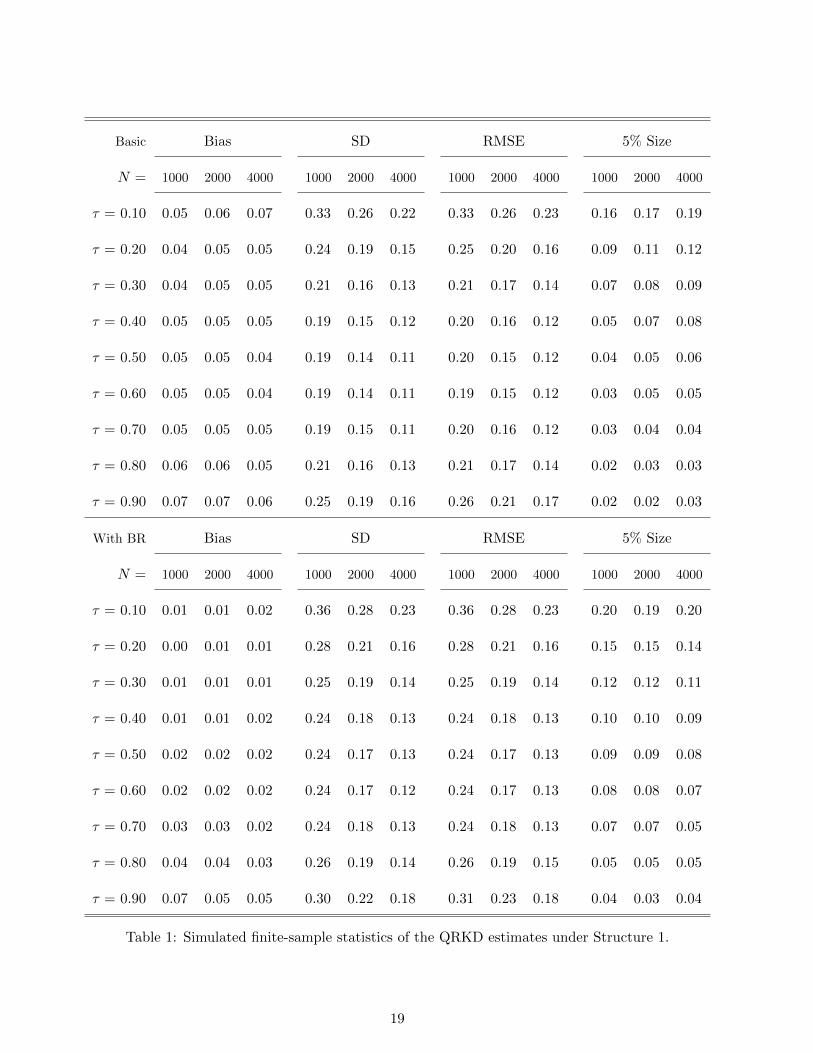
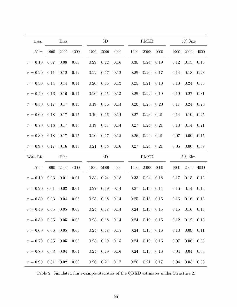
In order to more quantitatively analyze the finite sample pattern, we summarize some basic statis-

tics for the simulated distributions in Tables 1 and 2 for Structure 1 and Structure 2, respectively. In

each table, the four column groups list the absolute biases (Bias), the standard deviations (SD), root

mean squared errors (RMSE), and the rejection frequencies for point-wise 5%-level t-tests for the null

hypotheses of the true QRKD values (5% Size). The upper half of each table displays statistics for the

basic results, and the lower half of each table displays statistics for the results with bias reduction. For

each structure at each quantile τ , we again observe that SD and RMSE decrease as the sample size

N increases. These patterns are consistent with our previous discussions on Figures 1 and 2. Observe

that the 5% sizes are reasonably accurate at each quantile for each structure with bias reduction,

while they can increase without bias reduction as the sample size increases. We remark that the latter

15

fact does not contradict with our theory, because the practical choice of optimal bandwidth based on

an approximate MSE fails to under-smooth the estimates while our theory of asymptotic distribution

without bias reduction requires an under-smoothing.

While these sizes concern about point-wise inference, we also provide uniform inference results.

Figure 3 shows rejection probabilities for the 95% level uniform test of significance (panel A) and

the 95% level uniform test of heterogeneity (panel B) based on 1,000 iterations. Panel A shows that

the rejection probability for the test of the null hypothesis of insignificance does not increase in the

sample size for Structure 0, while it increases in the sample size for each of Structure 1 and Structure

2. Panel B shows that the rejection probability for the test of the null hypothesis of homogeneity does

not increase in the sample size for Structure 0 and Structure 1, while it increases in the sample size

for Structure 2. The above observations are consistent with the construction of Structure 0, Structure

1, and Structure 2.

5 An Empirical Illustration

In labor economics, causal effects of the unemployment insurance (UI) benefits on the duration of

unemployment are of interest from policy perspectives. The elasticity of labor supply with respect to

changes in unemployment insurance is an intertwining result of two endogenous forces – the liquidity

effects and the moral hazard effects. Landais (2015) demonstrates a reinterpretation of these forces in

terms of the traditional framework of dynamic labor supply, and shows how the moral hazard effects

of UI on search efforts can be explained by the Frisch elasticity concept, i.e., responses of search efforts

to changes in benefits keeping the marginal utility of wealth constant. He then proposes an empirical

strategy using the RKD to identify the moral hazard effects of UI. Using the data set of the Continuous

Wage and Benefit History Project (CWBH – see Moffitt, 1985), Landais estimates the effects of benefit

amounts on the duration of unemployment. In this section, we apply our QRKD methods, and aim to

discover potential heterogeneity in these causal effects. Using quantiles in this application also has an

16

Figure 1: Simulated distributions of QRKD estimates under Structure 1.

Basic Result; N = 1, 000 With BR; N = 1, 000

Basic Result; N = 2, 000 With BR; N = 2, 000

Basic Result; N = 4, 000 With BR; N = 4, 000

17

Figure 2: Simulated distributions of QRKD estimates under Structure 2.

Basic Result; N = 1, 000 With BR; N = 1, 000

Basic Result; N = 2, 000 With BR; N = 2, 000

Basic Result; N = 4, 000 With BR; N = 4, 000

18

Basic Bias SD RMSE 5% Size

N = 1000 2000 4000 1000 2000 4000 1000 2000 4000 1000 2000 4000

τ = 0.10 0.05 0.06 0.07 0.33 0.26 0.22 0.33 0.26 0.23 0.16 0.17 0.19

τ = 0.20 0.04 0.05 0.05 0.24 0.19 0.15 0.25 0.20 0.16 0.09 0.11 0.12

τ = 0.30 0.04 0.05 0.05 0.21 0.16 0.13 0.21 0.17 0.14 0.07 0.08 0.09

τ = 0.40 0.05 0.05 0.05 0.19 0.15 0.12 0.20 0.16 0.12 0.05 0.07 0.08

τ = 0.50 0.05 0.05 0.04 0.19 0.14 0.11 0.20 0.15 0.12 0.04 0.05 0.06

τ = 0.60 0.05 0.05 0.04 0.19 0.14 0.11 0.19 0.15 0.12 0.03 0.05 0.05

τ = 0.70 0.05 0.05 0.05 0.19 0.15 0.11 0.20 0.16 0.12 0.03 0.04 0.04

τ = 0.80 0.06 0.06 0.05 0.21 0.16 0.13 0.21 0.17 0.14 0.02 0.03 0.03

τ = 0.90 0.07 0.07 0.06 0.25 0.19 0.16 0.26 0.21 0.17 0.02 0.02 0.03

With BR Bias SD RMSE 5% Size

N = 1000 2000 4000 1000 2000 4000 1000 2000 4000 1000 2000 4000

τ = 0.10 0.01 0.01 0.02 0.36 0.28 0.23 0.36 0.28 0.23 0.20 0.19 0.20

τ = 0.20 0.00 0.01 0.01 0.28 0.21 0.16 0.28 0.21 0.16 0.15 0.15 0.14

τ = 0.30 0.01 0.01 0.01 0.25 0.19 0.14 0.25 0.19 0.14 0.12 0.12 0.11

τ = 0.40 0.01 0.01 0.02 0.24 0.18 0.13 0.24 0.18 0.13 0.10 0.10 0.09

τ = 0.50 0.02 0.02 0.02 0.24 0.17 0.13 0.24 0.17 0.13 0.09 0.09 0.08

τ = 0.60 0.02 0.02 0.02 0.24 0.17 0.12 0.24 0.17 0.13 0.08 0.08 0.07

τ = 0.70 0.03 0.03 0.02 0.24 0.18 0.13 0.24 0.18 0.13 0.07 0.07 0.05

τ = 0.80 0.04 0.04 0.03 0.26 0.19 0.14 0.26 0.19 0.15 0.05 0.05 0.05

τ = 0.90 0.07 0.05 0.05 0.30 0.22 0.18 0.31 0.23 0.18 0.04 0.03 0.04

Table 1: Simulated finite-sample statistics of the QRKD estimates under Structure 1.

19

Basic Bias SD RMSE 5% Size

N = 1000 2000 4000 1000 2000 4000 1000 2000 4000 1000 2000 4000

τ = 0.10 0.07 0.08 0.08 0.29 0.22 0.16 0.30 0.24 0.19 0.12 0.13 0.13

τ = 0.20 0.11 0.12 0.12 0.22 0.17 0.12 0.25 0.20 0.17 0.14 0.18 0.23

τ = 0.30 0.14 0.14 0.14 0.20 0.15 0.12 0.25 0.21 0.18 0.18 0.24 0.33

τ = 0.40 0.16 0.16 0.14 0.20 0.15 0.13 0.25 0.22 0.19 0.19 0.27 0.31

τ = 0.50 0.17 0.17 0.15 0.19 0.16 0.13 0.26 0.23 0.20 0.17 0.24 0.28

τ = 0.60 0.18 0.17 0.15 0.19 0.16 0.14 0.27 0.23 0.21 0.14 0.19 0.25

τ = 0.70 0.18 0.17 0.16 0.19 0.17 0.14 0.27 0.24 0.21 0.10 0.14 0.21

τ = 0.80 0.18 0.17 0.15 0.20 0.17 0.15 0.26 0.24 0.21 0.07 0.09 0.15

τ = 0.90 0.17 0.16 0.15 0.21 0.18 0.16 0.27 0.24 0.21 0.06 0.06 0.09

With BR Bias SD RMSE 5% Size

N = 1000 2000 4000 1000 2000 4000 1000 2000 4000 1000 2000 4000

τ = 0.10 0.03 0.01 0.01 0.33 0.24 0.18 0.33 0.24 0.18 0.17 0.15 0.12

τ = 0.20 0.01 0.02 0.04 0.27 0.19 0.14 0.27 0.19 0.14 0.16 0.14 0.13

τ = 0.30 0.03 0.04 0.05 0.25 0.18 0.14 0.25 0.18 0.15 0.16 0.16 0.18

τ = 0.40 0.05 0.05 0.05 0.24 0.18 0.14 0.24 0.19 0.15 0.15 0.16 0.16

τ = 0.50 0.05 0.05 0.05 0.23 0.18 0.14 0.24 0.19 0.15 0.12 0.12 0.13

τ = 0.60 0.06 0.05 0.05 0.24 0.18 0.15 0.24 0.19 0.16 0.10 0.09 0.11

τ = 0.70 0.05 0.05 0.05 0.23 0.19 0.15 0.24 0.19 0.16 0.07 0.06 0.08

τ = 0.80 0.03 0.04 0.04 0.24 0.19 0.16 0.24 0.19 0.16 0.04 0.04 0.06

τ = 0.90 0.01 0.02 0.02 0.26 0.21 0.17 0.26 0.21 0.17 0.04 0.03 0.03

Table 2: Simulated finite-sample statistics of the QRKD estimates under Structure 2.

20

(A) Rejection Probabilities for the 95% Level Test of Significance

Basic Result With Bias Reduction

(B) Rejection Probabilities for the 95% Level Test of Heterogeneity

Basic Result With Bias Reduction

Figure 3: Rejection probabilities for the 95% level uniform test of significance (panel A) and the 95%

level uniform test of heterogeneity (panel B) based on 1,000 replications.

21

advantage of informing a likely direction of the selection bias of the mean RKD estimator that stems

from not observing the mass of employed individuals at the low quantile (y = 0).

In all of the states in the United States, a compensated unemployed individual receives a weekly

benefit amount b that is determined as a fraction τ1 of his or her highest earning quarter x in the

base period (the last four completed calendar quarters immediately preceding the start of the claim)

up to a fixed maximum amount bmax, i.e. b = min{τ1 · x, bmax}. The both parameters, τ1 and

bmax, of the policy rule vary from state to state. Furthermore, the ceiling level bmax changes over

time within a state. For these reasons, empirical analysis needs to be conducted for each state for

each restricted time period. The potential duration of benefits is determined in a somewhat more

complicated manner. Yet, it also can be written as a piecewise linear and kinked function of a fraction

of a running variable x in the CWBH data set.

Following Landais (2015), we make our QRKD empirical illustration by using the CWBH data for

Louisiana. The data cleaning procedure is conducted in the same manner as in Landais. As a result

of the data processing, we obtain the same descriptive statistics (up to deflation) as those in Landais

for those variables that we use in our analysis. For the dependent variable y, we consider both the

claimed number of weeks of UI and the actually paid number of weeks. For the running variable x, we

use the highest quarter wage in the based period. The treatment intensity b is computed by using the

formula b(x) = min{(1/25) · x, bmax}, with a kink where the maximum amount is bmax = $4, 575 for

the period between September 1981 and September 1982 and bmax = $5, 125 for the period between

September 1982 and December 1983.

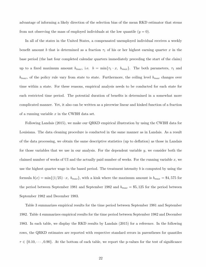
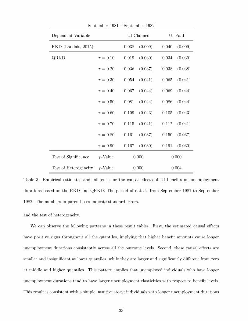
Table 3 summarizes empirical results for the time period between September 1981 and September

1982. Table 4 summarizes empirical results for the time period between September 1982 and December

1983. In each table, we display the RKD results by Landais (2015) for a reference. In the following

rows, the QRKD estimates are reported with respective standard errors in parentheses for quantiles

τ ∈ {0.10, · · · , 0.90}. At the bottom of each table, we report the p-values for the test of significance

22

September 1981 – September 1982

Dependent Variable UI Claimed UI Paid

RKD (Landais, 2015) 0.038 (0.009) 0.040 (0.009)

QRKD τ = 0.10 0.019 (0.030) 0.034 (0.030)

τ = 0.20 0.036 (0.037) 0.038 (0.038)

τ = 0.30 0.054 (0.041) 0.065 (0.041)

τ = 0.40 0.067 (0.044) 0.069 (0.044)

τ = 0.50 0.081 (0.044) 0.086 (0.044)

τ = 0.60 0.109 (0.043) 0.105 (0.043)

τ = 0.70 0.115 (0.041) 0.112 (0.041)

τ = 0.80 0.161 (0.037) 0.150 (0.037)

τ = 0.90 0.167 (0.030) 0.191 (0.030)

Test of Significance p-Value 0.000 0.000

Test of Heterogeneity p-Value 0.000 0.004

Table 3: Empirical estimates and inference for the causal effects of UI benefits on unemployment

durations based on the RKD and QRKD. The period of data is from September 1981 to September

1982. The numbers in parentheses indicate standard errors.

and the test of heterogeneity.

We can observe the following patterns in these result tables. First, the estimated causal effects

have positive signs throughout all the quantiles, implying that higher benefit amounts cause longer

unemployment durations consistently across all the outcome levels. Second, these causal effects are

smaller and insignificant at lower quantiles, while they are larger and significantly different from zero

at middle and higher quantiles. This pattern implies that unemployed individuals who have longer

unemployment durations tend to have larger unemployment elasticities with respect to benefit levels.

This result is consistent with a simple intuitive story; individuals with longer unemployment durations

23

September 1982 – December 1983

Dependent Variable UI Claimed UI Paid

RKD (Landais, 2015) 0.046 (0.006) 0.042 (0.006)

QRKD τ = 0.10 0.023 (0.028) 0.024 (0.028)

τ = 0.20 0.049 (0.034) 0.053 (0.034)

τ = 0.30 0.067 (0.038) 0.065 (0.038)

τ = 0.40 0.086 (0.040) 0.080 (0.040)

τ = 0.50 0.108 (0.041) 0.107 (0.041)

τ = 0.60 0.092 (0.040) 0.097 (0.040)

τ = 0.70 0.111 (0.038) 0.110 (0.038)

τ = 0.80 0.074 (0.034) 0.082 (0.034)

τ = 0.90 0.073 (0.027) 0.070 (0.027)

Test of Significance p-Value 0.026 0.021

Test of Heterogeneity p-Value 0.265 0.276

Table 4: Empirical estimates and inference for the causal effects of UI benefits on unemployment

durations based on the RKD and QRKD. The period of data is from September 1982 to December

1983. The numbers in parentheses indicate standard errors.

24

are associated with lower abilities and are therefore more likely to show moral hazard. The extent of

this increase of the causal effects in quantiles is more prominent for the results in Table 3 (1981–1982)

than in Table 4 (1982–1983). Under the assumption of rank invariance, this result unambiguously

implies that the moral hazard effects are heterogeneous. Without the rank invariance, one may want

to argue that the hetergeneous quantile treatment effects can be attributed to just heterogeneous

weights even without nonseparable heterogeneity. However, in the absence of nonseparability, the

weights would be also constant. Hence, our results show that there is nonseparable heterogeneity in

the causal structure even without the rank invariance. Third, the causal effects are very similar between

the results for claimed UI as the outcome and the results for paid UI as the outcome variable. The

respective standard errors are almost the same between these two outcome variables, but they are not

exactly the same. Fourth, the uniform tests show that the causal effects are significantly different from

zero for the both time periods. Lastly, the uniform tests show that the causal effects are significantly

heterogeneous in Table 3 (1981–1982), while the heterogeneity is insignificant in Table 4 (1982–1983).

The asymmetry in the last results may stem from different macro-economic environments between the

two time periods: the U.S. economy experienced a recession in most of the period 1981–1982 while it

was in recovery during the period 1982–1983.

6 Summary

Economists have taken advantage of policy irregularities to assess causal effects of endogenous treat-

ment intensities. A new approach along this line is the regression kink design (RKD) used by recent

empirical papers, including Nielsen, Sørensen and Taber (2010), Landais (2015), Simonsen, Skipper

and Skipper (2015), Card, Lee, Pei and Weber (2016), and Dong (2016). While the prototypical frame-

work is only able to assess the average treatment effect at the kink point, inference for heterogeneous

treatment effects using the RKD is of potential interest by empirical researchers (e.g., Landais (2011)

considers it). In this light, this paper develops causal analysis and methods for the quantile regression

25

kink design (QRKD).

We first develop causal interpretations of the QRKD estimand. It is shown that the QRKD

estimand measures the marginal effect of the treatment variable on the outcome variable at the

conditional quantile of the outcome given the design point of the running variable provided that the

causal structure exhibits rank invariance. This result is generalized to the case of no rank invariance,

where the QRKD estimand is shown to measure a weighted average of the marginal effects of the

treatment variable on the outcome variable at the conditional quantile of the outcome given the design

point of the running variable. Second, we propose a sample counterpart QRKD estimator, and develop

its asymptotic properties for statistical inference of heterogeneous treatment effects. Using uniform

Bahadur representations, we obtain a weak consistency result for the QRKD estimator. Applying

the weak consistency result, we propose procedures for statistical tests of treatment significance and

treatment heterogeneity. Simulation studies support our theoretical results. Applying our methods to

the Continuous Wage and Benefit History Project (CWBH) data, we find significantly heterogeneous

causal effects of unemployment insurance benefits on unemployment durations in the state of Louisiana

for the period between September 1981 and September 1982. Finally, while the main text mostly

focuses on the sharp QRKD that is relevant to our empirical illustration, we remark that identification

and estimation results for the fuzzy QRKD are also available in Section A in the supplementary

appendix for completeness.

References

Angrist, Joshua D. and Guido W. Imbens (1995) “Two-Stage Least Squares Estimation of Average

Causal Effects in Models with Variable Treatment Intensity,” Journal of the American Statistical

Association, Vol. 90, No. 430, pp. 431–442.

Card, David, David Lee, Zhuan Pei, and Andrea Weber (2016) “Inference on Causal Effects in a

Generalized Regression Kink Design,” Econometrica, Vol. 83, No. 6, pp. 2453–2483.

26

Calonico, Sebastian, Matias D. Cattaneo, and Rocio Titiunik (2014) “Robust Nonparametric Confi-

dence Intervals for Regression-Discontinuity Designs,” Econometrica, Vol. 82, No. 6, pp. 2295–2326.

Chernozhukov, Victor and Ivan Fernandez-Val (2005) “Subsampling Inference on Quantile Regression

Processes,” Sankhya: The Indian Journal of Statistics, Vol. 67, No. 2, pp. 253–276.

Dong, Yingying (2016) “Jump or Kink? Identifying Education Effects by Regression Discontinuity

Design without the Discontinuity,” Working Paper.

Frandsen, Brigham R., Markus Frolich and Blaise Melly (2012) “Quantile Treatment Effects in the

Regression Discontinuity Design,” Journal of Econometrics, Vol. 168, No.2 pp. 382-395.

Gine, Evarist and Richard Nickl (2015) “Mathematical Foundations of Infinite-Dimensional Statistical

Models,” Cambridge University Press: Cambridge.

Guerre, Emmanuel and Camille Sabbah (2012) “Uniform Bias Study and Bahadur Representation for

Local Polynomial Estimators of the Conditional Quantile Function,” Econometric Thoery, Vol. 26,

No. 5, pp. 1529-1564.

Imbens, Guido W. and Joshua D. Angrist (1994) “Identification and Estimation of Local Average

Treatment Effects,” Econometrica, Vol. 62, No. 2, pp. 467–475.

Imbens, Guido and Thomas Lemieux (2008) “Special Issue Editors’ Introduction: The Regression

Discontinuity Design – Theory and Applications,” Journal of Econometrics, Vol. 142, No. 2, pp.

611–614.

Imbens, Guido W. and Jeffrey M. Wooldridge (2009) “Recent Developments in the Econometrics of

Program Evaluation,” Journal of Economic Literature, Vol. 47, No. 1, pp. 5–86.

Koenker, Roger and Zhijie Xiao (2002) “Inference on the quantile regression process,” Econometrica,

Vol. 70, No. 4, pp.1583–1612.

27

Kong, Efang, Oliver B. Linton, and Yingcun Xia (2010) “Uniform Bahadur Representation for Local

Polynomial Estimates of M-Regression and its Application to the Additive Model?,” Econometric

Thoery, Vol. 26, No. 5, pp. 1529-1564.

Landais, Camille (2011) “Heterogeneity and Behavioral Responses to Unemployment Benefits over

the Business Cycle,” Working Paper, LSE.

Landais, Camille (2015) “Assessing the Welfare Effects of Unemployment Benefits Using the Regression

Kink Design,” American Economic Journal: Economic Policy, Vol. 7, No. 4, pp. 243–278.

Lee, David S., and Thomas Lemieux (2010) “Regression Discontinuity Designs in Economics,” Journal

of Economic Literature, Vol. 48, No. 2, pp. 281–355.

Moffitt, Robert (1985) “The Effect of the Duration of Unemployment Benefits on Work Incentives:

An Analysis of Four Datasets,” Unemployment Insurance Occasional Papers 85-4, U.S. Department

of Labor, Employment and Training Administration.

Nielsen, Helena Skyt, Torben Sørensen, and Christopher Taber (2010) “Estimating the Effect of

Student Aid on College Enrollment: Evidence from a Government Grant Policy Reform,” American

Economic Journal: Economic Policy, Vol. 2, No. 2, pp. 185–215.

Qu, Zhongjun and Jungmo Yoon (2015a) “Nonparametric Estimation and Inference on Conditional

Quantile Processes,” Journal of Econometrics, Vol. 185, No.1 pp. 1-19.

Qu, Zhongjun and Jungmo Yoon (2015b) “Uniform Inference on Quantile Effects under Sharp Re-

gression Discontinuity Designs,” Working Paper, 2015.

Sabbah, Camille (2014) “Uniform Confidence Bands for Local Polynomial Quantile Estimators,”

ESAIM: Probability and Statistics, Vol. 18, pp. 265-276.

Sasaki, Yuya (2015) “What Do Quantile Regressions Identify for General Structural Functions?,”

Econometric Thoery, Vol. 31, No. 5, pp. 1102-1116.

28

Simonsen, Marianne, Lars Skipper, and Niels Skipper (2015) “Price sensitivity of demand for prescrip-

tion drugs: Exploiting a regression kink design,” Journal of Applied Econometrics, Forthcoming.

29

Supplementary Appendix to

“Causal Inference by Quantile Regression Kink Designs”

Harold D. Chiang Yuya Sasaki

Johns Hopkins University

August 30, 2016

This supplementary appendix provides extensions to and details of the contents presented in the

main text. The appendix consists of three sections. First, we extend our identification and estimation

results for sharp quantile regression kink designs (QRKD) to fuzzy QRKD in Section A. Second,

Section B contains mathematical appendix including auxiliary lemmas, their proofs, and proofs for

the results presented in the main text. Third, we present practical procedures in Section C.

A Extension to Fuzzy QRKD

A.1 Causal Interpretation of the Fuzzy QRKD

While Section 2.2 in the main text focuses on the case of sharp QRKD, our identification result

(Theorem 1) can be extended to the case of fuzzy QRKD in an analogous manner to the corresponding

extension in Card, Lee, Pei and Weber (2016). In the current appendix section, we show the causal

interpretation for the fuzzy QRKD.

The fuzzy QRKD estimand reads as

limx↓x0∂∂xQY |X(τ | x)− limx↑x0

∂∂xQY |X(τ | x)

limx↓x0∂∂xE[B | X = x]− limx↑x0

∂∂xE[B|X = x]

,

1

where B denotes the random variable for the treatment intensity. Unlike the sharp case, it is not

deterministically controlled by the running variable. With the M -dimensional unobservables ε =

(ε1, ε2) decomposed into two parts, we specify the relevant causal structure by

y = g(b, x, ε2)

b = b(x, ε1)

For short-hand notations, we write b1(x, ε1) = ∂∂xb(x, ε1) and h(x, ε) = g(b(x, ε1), x, ε2). With these

notations under the above setup, we make the following assumption.

Assumption 7. (a) b( · , ε1) is continuous on X and continuously differentiable on X \{x0} for all ε1.

(b) There exist an absolutely integrable function that envelops b1(x, ·) for all x. (c) E[(b1(x+0 , ε1) −

b1(x−0 , ε1))|X = x0] and∫

(b1(x+0 , ε1) − b1(x−0 , ε1))dµy,x0(ε) exist and are finite and nonzero, where

µy,x0 is defined as in Section 2.2.

Under this assumption, together with the basic assumptions from Section 2.2, we obtain the

following causal interpretation of the fuzzy QRKD estimand by similar lines of proof to those of

Theorem 1.

Theorem 3. Suppose that Assumptions 2 (with the modified definitions of g, h and ε in the current

appendix section), 3, 4, 5 and 7 are satisfied. For each y ∈ Y, we have

limx↓x0∂∂xQY |X(τ | x)− limx↑x0

∂∂xQY |X(τ | x)

limx↓x0∂∂xE[B | X = x]− limx↑x0

∂∂xE[B|X = x]

= χ

∫g1(b(x0, ε1), x0, ε2)dψy,x0(ε1, ε2) = χEψy,x0 [g1(b(x0, ε1), x0, ε2)]

where τ = FY |X(y | x0), χ =∫

(b1(x+0 ,ε1)−b1(x−0 ,ε1))dµy,x0 (ε)∫(b1(x+0 ,ε1)−b1(x−0 ,ε1))dFε(ε)

, and ψy,x0(S) =∫S(b1(x+0 ,ε1)−b1(x−0 ,ε1))dµy,x0 (ε)∫(b1(x+0 ,ε1)−b1(x−0 ,ε1))dµy,x0 (ε)

for all S ∈ B(y, x).

This result shows that the fuzzy QRKD estimand equals a constant χ times a weighted average of

the marginal effects. The presence of the constant term χ somewhat obscures the causal interpretation

2

of the estimand. In case where the kink direction is uniform, i.e., b1(x+0 , ε1)− b1(x−0 , ε1) has the same

sign for all ε1, the sign of χ is positive, and so the sign of the fuzzy QRKD can be considered to

measure the sign of the weighted average marginal effects. A working paper version of Sasaki (2015)

implies that µy,x0 = Fε holds if g takes the following semi-separable form

g(b(x, ε1), x, ε2) = gI(b(x, ε1), x) + gII(x, ε2).

In this case, we have χ = 1 and therefore the fuzzy QRKD can be interpreted as a weighted average

of marginal effects without worrying about the multiplying constant.

A.2 Estimation and Asymptotics for the Fuzzy QRKD

The main text focuses on the sharp QRKD. In this appendix, we provide an estimator for the fuzzy

QRKD estimand developed in Appedix A.1 and its asymptotic properties. The conditional mean

of the policy with errors, b(X, ε1), is written as m(x) = E[b(X, ε1)|X = x]. The regression is also

represented by the canonical decomposition B = m(X)+U , where the error U satisfies E[U |X = 0] = 0

and V (U |X = x) = σ2(x). The fuzzy QRKD estimand can then be estimated by

QRKDf (τ) =β+(τ)− β−(τ)

m′(x+0 )− m′(x−0 )

,

where the numerator is the same as the one in Section 3 in the main text. For denominator, we use

the local derivative estimator

m′(x+0 ) =

− 1nh2n

∑ni=1 biK

′(xi−x0hn)d+i − m(x+

0 )(− 1

nh2n

∑ni=1K

′(xi−x0hn)d+i

)1nhn

∑ni=1K(xi−x0hn

)d+i

where m(x+0 ) =

∑ni=1 biK(xi−x0hn

)d+i /∑n

i=1K(xi−x0hn)d+i , as in Equation (4.14) of Pagan and Ullah

(1999). The left counterpart, m′(x−0 ), can be defined analogously. Notice that we are using hn as

the bandwidth for m′(x+0 ). This is reasonable for the asymptotic argument because, as we will see,

m′(x+0 ) and β+(τ) have the same rate of convergence. We make the following assumptions.

Assumption 8.

(i) The partial derivatives of fX , m and∫b2fBX(b, · )db exist up to the third order and are bounded.

3

(ii) There exists a δ > 0 such that E[|U |2+δ | X = x0] <∞ and∫|K(u)|2+δ <∞.

(iii) ‖K ′‖∞ <∞.

(iv) fY XB exists and is continuous in x for each (y, b) ∈ R2. Also, there exists a > 0 such that

|m′(x+0 )−m′(x−0 )| > a.

(v) There exists an x such that Q(τ |·) is monotone on (x0, x).

Theorem 4. Under Assumptions 6, 7, and 8, we have

√nh3

n( QRKDf (τ)−QRKDf (τ))⇒ (m′(x+0 )−m′(x−0 ))G∆(τ)− (β+(τ)− β−(τ))G∆(b)

(m′(x+0 )−m′(x−0 ))2

,

where G∆ is a Gaussian process with mean zero and covariance function as following: for any

given r, s, τ ∈ T and let b stand for the dimension of m′(x), Cov(G∆(b), G∆(b)) = σ+b,b + σ−b,b,

Cov(G∆(τ), G∆(b)) = σ+τ,b + σ−τ,b, Cov(G∆(r), G∆(s)) = σ+

r,s + σ−r,s, where

σ+b,b =

σ2(x0)

fX(x0)

∫K ′(v)2dv,

σ+τ,b =

ι′2(N+)−1√c(τ)fX(x0)2fY |X(Q(τ |x+

0 )|x+0 )

∫R

∫R

∫(0,∞)

(τ − 1{y ≤ Q(τ |x0)})(1, v

c(τ))′

×K(v

c(τ))K ′(v)(b− E[b(X, E1)|X = x0])fY XB(y, x0 + hnv, b)dvdydb,

σ+r,s =

c(1/2)

c(r)c(s)fX(x0)fY |X(Q(r|x+0 )|x0)fY |X(Q(s|x+

0 )|x0)(r ∧ s− rs)ι′2(N+)−1T+(r, s)(N+)−1ι2,

and the left counterparts are defined analogously.

A proof of this theorem is provided in Section B.8.

B Mathematical Appendix

In addition to those notations introduced in the main text, we define the linear extrapolation error

ei =[Q(τ |x+

0 ) + (xi − x0)∂Q(τ |x+0 )

∂x

]− Q(τ |xi) and the estimation errors φ(τ) =

√nhn,τ [α+(τ) −

Q(τ |x+0 ), hn,τ (β+(τ) − ∂Q(τ |x+0 )

∂x )]′. Although they are not direct objects of interest, the level es-

timators are denoted by α+(τ) = ι′1 arg minα,β

∑ni=1 d

+i K(xi−x0hn,τ

)ρτ (yi − α − β(xi − x0)) and α−(τ) =

4

ι′1 arg minα,β

∑ni=1 d

−i K(xi−x0hn,τ

)ρτ (yi−α−β(xi−x0)), where ι1 = [1, 0]′. We also use short-hand notations

z′i,n,τ = (1, (xi − x0)/hn,τ ) and Ki,n,τ = K(xi−x0hn,τ).

B.1 Auxiliary Lemmas: Uniform Consistency

In this appendix section, we develeop the following auxiliary results that show uniform convergences

of some useful local sample moments over T . While it is stated for right observations only, we remark

that similar results hold for left observations too.

Lemma 1. Under Assumption 6, we have

(i) (nhn,τ )−1∑n

i=1Ki,n,τzi,n,τz′i,n,τd

+i

P−→ fX(x0)N+ uniformly in τ ∈ T ;

(ii) (nhn,τ )−1∑n

i=1 fY |X(yi|xi)Ki,n,τzi,n,τz′i,n,τd

+i

P−→ fY |X(Q(τ |x+0 )|x+

0 )fX(x0)N+ uniformly in τ ∈ T

with any yi lying between Q(τ |xi) and Q(τ |xi) + ei(τ) + (nhn,τ )−1/2z′i,n,τd+i φ(τ) for each i;

(iii) (nh3n,τ )−1

∑ni=1

12

(xi−x0hn,τ

)2 ∂2Q(τ |x+0 )

∂x2h2n,τzi,n,τKi,n,τd

+i

P−→ fX(x0)2

∫∞0 u2 ∂

2Q(τ |x+0 )

∂x2(1, u)′K(u)du uni-

formly in τ ∈ T .

Proof. (i): We claim E[(nhn,τ )−1

∑ni=1Ki,n,τzi,n,τz

′i,n,τd

+i

]→ fX(x0)N+ uniformly in τ ∈ T and

(nhn,τ )−1∑n

i=1Ki,n,τzi,n,τz′i,n,τd

+i

p−→ E[(nhn,τ )−1

∑ni=1Ki,n,τzi,n,τz

′i,n,τd

+i

]uniformly in τ ∈ T. We

provide a proof for only ι′2(nhn,τ )−1∑n

i=1Ki,n,τzi,n,τz′i,n,τ ι2 = (nhn,τ )−1

∑ni=1

(xi−x0hn,τ

)2K(xi−x0hn,τ

). Sim-

ilar arguments apply for the other simpler entries.

First note that, by Assumption 6 (i)(a), (i) (b), (iv), and (v),

Eι′2(nhn,τ )−1n∑i=1

Ki,n,τzi,n,τz′i,n,τd

+i ι2 =

∫ ∞0

u2K(u){fX(x0) + f ′(x0)uhn,τ + o(uhn,τ )}du.

Assumption 6 (i) (a) implies that f ′X(x) is bounded in a neighbourhood of x0. Assumption 6 (iv)

and (v) then implies that the right-hand side in the equation above is fX(x0)ι′2N+ι2 +O(hn,τ ). Since

O(hn,τ ) = O(c(τ)hn) = O(chn), the convergence is uniform in τ ∈ T .

In the remainder, we show the uniform convergence of the stochastic part using empirical process

theories. We denote sup{supp(K)} = k. Let F = {xi 7→ a2(xi−x0)2

c(τ)31{K(a(xi−x0)

c(τ) ) > 0}K(a(xi−x0)

c(τ)

)1{xi ≥

5

x0} : (τ, a) ∈ T × [0,∞)}. Because each f ∈ F is right continuous under (iv) of Assumption 6, this

family is a point-wise measurable class – see Einmahl and Mason (2005) and Section 2.3 of van der

Vaart and Wellner (1996). For each (τ, a) ∈ {T × [0,∞), xi 7→ a2(xi−x0)2

c(τ)21{K(a(xi−x0)

c(τ) ) > 0} is mono-

tone on its support and bounded by k2 under (iv) of Assumption 6. Meanwhile, c(τ) is finite and

bounded away from 0 uniformly in τ ∈ T under (v) of Assumption 6, and so is (1/c(τ)). Therefore,

xi 7→ a2(xi−x0)2

c(τ)31{K(a(xi−x0)

c(τ) ) > 0} is of bounded variation. xi 7→ 1{xi ≥ x0} is trivially of bounded

variation. Putting them together, we have that each element in F is of bounded variation with a

measurable envelope F (xi) =k2‖K‖∞

c , where the constant c is from (v) of Assumption 6. Since F is a

finite constant, ‖F‖2P,2 =∫|F |2fX(xi)dxi = P |F |2 <∞. Without loss of generality as it is bounded,

we can assume F ≤ 1. By Theorem 3.6.12 of Gine and Nickl (2016), F is of VC-type (Euclidean),

that is to say that there exists constant k, v < ∞ such that supQ logN(ε ‖F‖Q,2 ,F , L2(Q)) ≤ (kε )v

for 0 < ε ≤ 1 and for all probability measures Q supported on supp(X).

This implies the uniform entropy integral J(1,F , F ) = supQ∫ 1

0

√1 + logN(ε ‖F‖Q,2 ,F , L2(Q))dε <

∞. Since F ∈ L2(P ), we can apply Theorem 5.2 of Chernozhukov, Chetverikov and Kato (2014) to

obtain

E

[supf∈F

∣∣∣∣ 1√n

n∑i=1

f(Xi)−∫fdP

∣∣∣∣] ≤ C{J(1,F , F ) ‖F‖P,2 +BJ2(1,F , F )

δ2√n

} <∞

with B =√

max1≤i≤n F (Xi) <∞ and an universal constant C > 0.

Multiplying both sides by (√nhn)−1 yields

E

[supτ∈T

∣∣∣∣(nhn,τ )−1n∑i=1

(xi − x0

hn,τ

)2K(xi − x0

hn,τ

)d+i − E

[(nhn,τ )−1

n∑i=1

(xi − x0

hn,τ

)2K(xi − x0

hn,τ

)d+i

]∣∣∣∣]

≤ 1√nhn,τ

C{J(1,F , F ) ‖F‖P,2 +BJ2(1,F , F )

δ2√n

}.

Thus, the right hand side goes to 0 if nh2n,τ → ∞ as n → ∞. Finally, Markov inequality gives the

desired result.

(ii): As in the proof of part (i), we show E[(nhn,τ )−1

∑ni=1 fY |X(yi|xi)Ki,n,τzi,n,τz

′i,n,τd

+i

]→

fY |X(Q(τ |x+0 )|x+

0 )fX(x0)N+ uniformly in τ ∈ T , and then we also show (nhn,τ )−1∑n

i=1 fY |X(yi|xi)

6

Ki,n,τzi,n,τz′i,n,τd

+i

p−→ E[(nhn,τ )−1

∑ni=1 fY |X(yi|xi)Ki,n,τzi,n,τz

′i,n,τd

+i

]uniformly in τ ∈ T .

First we bound |Q(τ |xi) − (Q(τ |xi) + ei(τ) + (nhn,τ )−1/2z′i,n,τ φ(τ))|1{K(xi−x0hn,τ) > 0} = |ei(τ) +

(nhn,τ )−1/2z′i,n,τ φ(τ)|1{K(xi−x0hn,τ) > 0}. Following part 1 of the proof of Theorem 1 in Qu and Yoon

(2015a), and using part (i) of our Lemma 1, we have φ(τ) ≤√

log nhn with probability approaching one

uniformly in τ ∈ T . Therefore, under Assumption 6 (iv) and (v), we have (nhn,τ )−1/2z′i,n,τ φ(τ)1{K(xi−x0hn,τ) >

0} = Op(√

lognhnnhn

) uniformly in i and τ ∈ T .

We next bound ei(τ)1{K(xi−x0hn,τ) > 0} = {

[Q(τ |x+

0 ) + (xi − x0)∂Q(τ |x+0 )

∂x

]−Q(τ |xi)}1{K(xi−x0hn,τ

) >

0}. By the mean value expansion of Q(τ |xi) at x = x0 +δ and let x→ x+0 , we have ei(τ)1{K(xi−x0hn,τ

) >

0} = [∂Q(τ |x+0 )

∂x − ∂Q(τ |x)∂x ](xi− x0)1{K(xi−x0hn,τ

) > 0} ≤M ‖(τ, x0)− (τ, x)‖ (xi− x0)1{K(xi−x0hn,τ) > 0} ≤

M ‖(maxT, x0)− (minT, x)‖O(hn) = O(hn) uniformly in τ ∈ T for some constant M by Lipschitz

continuity and properties of bandwidth from Assumption 6 (iii) (a), (iii) (b) and (iv).

Similarly, we can bound |Q(τ |x+0 ) − Q(τ |xi)|1{K(xi−x0hn,τ

) > 0}. By the joint Lipschitz continuity

from Assumption 6 (iii)(a)(b), we have |Q(τ |x+0 )−Q(τ |xi)|1{K(xi−x0hn,τ

) > 0} ≤M ‖(x0, τ)− (xi, τ)‖ =

O(hn) uniformly in τ ∈ T for some constant M .

Combing the auxiliary results above, we have |Q(τ |xi) − yi|1{K(xi−x0hn,τ) > 0} ≤ |Q(τ |xi) −

(Q(τ |xi) + ei(τ) + (nhn,τ )−1/2z′i,n,τ φ(τ))|1{K(xi−x0hn,τ) > 0} = Op(

√lognhnnhn

) + O(hn) and |Q(τ |x+0 ) −

Q(τ |xi)|1{K(xi−x0hn,τ) > 0} ≤ 1} = O(hn) uniformly in i and in τ ∈ T . By the triangle inequality,

|Q(τ |x+0 )− yi|1{K(xi−x0hn,τ

) > 0} ≤ Op(√

lognhnnhn

) +O(hn) uniformly in i and τ ∈ T .

Using Assumption 6 (i) (a), (i) (b), (ii) (a) and (iv) along with the asymptotic bounds obtained

above,

Eι′2(nhn,τ )−1n∑i=1

fY |X(yi|xi)Ki,n,τzi,n,τz′i,n,τd

+i ι2

=fY |X(Q(τ |x+0 )|x+

0 )fX(x0)ι′2N+ι2 +Op((log nhn/nhn)1/2) +O(hn)

holds uniformly in τ ∈ T . Convergence of the other entries follows similarly.

For the second part, let F = { xi 7→a2(xi−x0)2fY |X(b|xi)

c(τ)31{K

(a(xi−x0)c(τ)

)> 0}K

(a(xi−x0)c(τ)

)1{xi ≥

7

x0} : (τ, a, b) ∈ T × [0,∞) × [inf(τ,x)∈T×(x0,x]Q(τ |x), sup(τ,x)∈T×(x0,x]Q(τ |x)] }. Notice that the

interval of infimum and supremum is bounded by Assumption 6 (iii) (b). An argument similar

to the proof of (i) shows that each element in F is of bounded variation with a measurable en-

velope F (xi) =k2‖K‖∞ sup(y,x) fY |X

c , where the supremum in the numerator is taken over (x, y) ∈

(x0, x] × [inf(τ,x)∈T×(x0,x]Q(τ |x), sup(τ,x)∈T×(x0,x]Q(τ |x)], under parts (ii), (iv) and (v) of Assump-

tion 6. Using the VC-type class argument and applying the same inequality from Chernozhukov,

Chetverikov and Kato (2014) provides a bound for expectation that goes to zero if nh2n → 0. Markov

inequality then gives the desired result.

(iii): We focus on the entry ι′2(nh3n,τ )−1

∑ni=1

12

(xi−x0hn,τ

)2 ∂2Q(τ |x+0 )

∂x2h2n,τzi,n,τKi,n,τd

+i ι2. Similar argu-

ments apply to the other entries. The process is similar to (i). The deterministic part can be shown by

computing the expectation. For the stochastic part, let F = {xi 7→ a3(xi−x0)3

c(τ)4∂2Q(τ |x+0 )

∂x21{K(a(xi−x0)

c(τ) >

0}K(a(xi−x0)

c(τ)

)1{xi ≥ x0} : (τ, a) ∈ T × [0,∞)} is a VC type class with a measurable envelope

F (xi) =k3m‖K‖∞

c where m = supT∂2Q(τ |x+0 )

∂x2< ∞ under Assumption 6 (iii)(b) and T is compact.

Then the same uniform consistency argument applies under parts (iii) (a) (b), (iv) and (v) of Assump-

tion 6. The same inequality from Chernozhukov, Chetverikov and Kato (2014) and Markov inequality

give the desired result.

Following similar reasoning, we also have the corresponding results for uniform convergences of

some local moments for local quadratic regression.

Lemma 2. Under Assumption 6, 9, we have

(i) (nhn,τ )−1∑n

i=1 Ki,n,τ zi,n,τ z′i,n,τd

+i

P−→ fX(x0)N+ uniformly in τ ∈ T ;

(ii) (nhn,τ )−1∑n

i=1 fY |X(yi|xi)Ki,n,τ zi,n,τ z′i,n,τd

+i

P−→ fY |X(Q(τ |x+0 )|x+

0 )fX(x0)N+ uniformly in τ ∈ T

with any yi lying between Q(τ |xi) and Q(τ |xi) + ei(τ) + (nhn,τ )−1/2z′i,n,τd+i

ˆφ(τ) for each i, where

ˆφ(τ) =√nhn,τ [α+(τ) − Q(τ |x+

0 ), hn,τ (β+(τ) − ∂Q(τ |x+0 )∂x ), h2

n,τ (λ+(τ) − 12∂2Q(τ |x+0 )

∂x2)]′ and ei(τ) =

[Q(τ |x+0 ) + (xi − x0)

∂Q(τ |x+0 )∂x + (xi − x0)2 ∂

2Q(τ |x+0 )

∂x2]−Q(τ |xi) ;

(iii) (nh4n,τ )−1

∑ni=1

13!

(xi−x0hn,τ

)3 ∂3Q(τ |x+0 )

∂x3h3n,τ zi,n,τ Ki,n,τd

+i

P−→ fX(x0)3!

∫∞0 u3 ∂

3Q(τ |x+0 )

∂x3[1, u, u2]′K(u)du

8

uniformly in τ ∈ T .

B.2 Uniform Bahadur Representation

Lemma 3. Under Assumption 6, we have

√nh3

n,τ

(β+(τ)− ∂Q(τ |x+

0 )

∂x− hn,τ

ι′2(N+)−1

2

∫ ∞0

u2∂2Q(τ |x+

0 )

∂x2(1, u)′K(u)du

)=ι′2(N+)−1(nhn,τ )−

12∑n

i=1(τ − 1{yi ≤ Q(τ |xi)})zi,n,τKi,n,τd+i )

fX(x0)fY |X(Q(τ |x+0 )|x+

0 )+ op(1)

uniformly in τ ∈ T. Similar results hold for β−(τ).

A proof is provided below – auxiliary results of uniform consistency that are used to prove this

theorem are also provided in Section B.1 in the supplementary appendix. The Bahadur representation

obtained in this lemma is uniform in quantiles τ ∈ T for a fixed location of the running variable x.

Kong, Linton and Xia (2010) derived a Bahadur representation that is uniform in x for a fixed quantile

level. Guerre and Sabbah (2012) derived a result that is uniform in both τ and x for interior points

– see also Sabbah (2014). Since we are interested in a representation at the boundary point x0 of

the truncated distribution, and since we did not require the uniformity in x, and we developed our

approach more closely following Qu and Yoon (2015a).

Proof. For this lemma, we mostly follow the proof of Theorem 1 in Qu and Yoon (2015a). The major

difference is that we focus on the second coordinate of φ instead of the first one. By step 1 of the

proof of Theorem 1 in Qu and Yoon (2015a) which is applicable under parts (i), (ii) (a), (ii) (b), (iii)

(a), (iii) (b), (iv) and (v) of our Assumption 6, we have supτ∈T ‖φ(τ)‖ ≤ (log nhn)1/2 with probability

approaching one as n→∞. Asymptotically, therefore, we only need to focus on studying the behavior

of the subgradient

(subgradient) =

n∑i=1

{τ − 1(u0i (τ) ≤ ei(τ) + (nhn,τ )−1/2z′i,n,τ φ(τ))}zi,n,τKi,n,τd

+i

on the set Φn = {(τ, φ(τ)) : τ ∈ T, ‖φ(τ)‖ ≤ log1/2(nhn)}, where u0i (τ) = yi − Q(τ |xi) and ei(τ) =

9

[Q(τ |x+

0 ) + (xi − x0)∂Q(τ |x+0 )

∂x

]−Q(τ |xi). Denote

Sn(τ, φ(τ), ei(τ)) = (nhn)−1/2n∑i=1

{P ((u0i (τ) ≤ ei(τ) + (nhn,τ )−1/2z′i,n,τφ(τ))|xi)

−1(u0i (τ) ≤ ei(τ) + (nhn,τ )−1/2z′i,n,τφ(τ))}zi,n,τKi,n,τd

+i .

Theorem 2.1 of Koenker (2005) and Assumption 6 (iv) imply (nhn)−1/2·(subgradient) = Op((nhn)−1/2)

uniformly in τ ∈ T.

Following Qu and Yoon (2015a), we can rewrite the subgradient (scaled by (nhn)−1/2) as

(nhn)−1/2n∑i=1

{τ − 1(u0i (τ) ≤ ei(τ) + (nhn,τ )−1/2z′i,n,τ φ(τ))}zi,n,τKi,n,τd

+i

={Sn(τ, φ(τ), ei(τ))− Sn(τ, 0, ei(τ))}+ {Sn(τ, 0, ei(τ))− Sn(τ, 0, 0)}+ Sn(τ, 0, 0)

+(nhn)−1/2n∑i=1

{τ − P ((u0i (τ) ≤ ei(τ) + (nhn,τ )−1/2z′i,n,τ φ(τ)|xi)}zi,n,τKi,n,τd

+i

The differences inside the first two pairs of curly brackets are of order op(1) on the set Φn by Lemma

B5 of Qu and Yoon (2015a), which is applicable under parts (i), (ii) (a), (ii) (b), (iii) (a), (iii) (b), (iv)

and (v) of our Assumption 6. The Sn(τ, 0, 0) term is Op(1) under Assumption 6 (i) (a), (iv), (v). The

conditional probability in the last term is a conditional CDF of Y |X. Applying the first order mean

value expansion to the last term at y = Q(τ |xi) yields

(nhn)−1/2n∑i=1

{τ − P ((u0i (τ) ≤ ei(τ) + (nhn,τ )−1/2z′i,n,τ φ(τ)|xi)}zi,n,τKi,n,τd

+i

=− (nhn)−1/2n∑i=1

fY |X(yi|xi)ei(τ)zi,n,τKi,n,τd+i

− (nhn)−1/2(nhn,τ )−1/2( n∑i=1

fY |X(yi|xi)Ki,n,τzi,n,τz′i,n,τd

+i

)φ(τ),

where yi lies between Q(τ |xi) and Q(τ |xi) + ei(τ) + (nhn,τ )−1/2z′i,n,τd+i φ(τ).

Taking the above auxiliary results together, we can now rewrite subgradient (scaled by (nhn)−1/2)

as

Sn(τ, 0, 0)− (nhn)−1/2n∑i=1

fY |X(yi|xi)ei(τ)zi,n,τKi,n,τd+i

− (nhn)−1/2(nhn,τ )−1/2( n∑i=1

fY |X(yi|xi)Ki,n,τzi,n,τz′i,n,τd

+i

)φ(τ).

10

Recall that this subgradient (scaled by (nhn)−1/2) is op(1) uniformly in τ ∈ T .

By Lemma 1 (ii), (nhn,τ )−1∑n

i=1 fY |X(yi|xi)Ki,n,τzi,n,τz′i,n,τd

+i

P−→ fY |X(Q(τ |x+0 )|x+

0 )fX(x0)N+

uniformly in τ ∈ T and so

Sn(τ, 0, 0)− (nhn)−1/2n∑i=1

fY |X(yi|xi)ei(τ)zi,n,τKi,n,τd+i

=(hn,τhn

)1/2[fY |X(Q(τ |x+

0 )|x+0 )fX(x0)N+ + op(1)

]φ(τ) + op(1)

uniformly in τ ∈ T . Since N+ is positive definite and fY |X(Q(τ |x+0 )|x+

0 )fX(x0) > 0 by parts (i), (ii)

(b) and (iv) of Assumption 6, we obtain

φ(τ) =(fX(x0)fY |X(Q(τ |x+

0 )|x+0 )N+ + op(1)

)−1×[(hnhn,τ

)1/2

Sn(τ, 0, 0)− (nhn,τ )−1/2fY |X(Q(τ |x+0 )|x+

0 )n∑i=1

ei(τ)zi,n,τKi,n,τd+i + op(1)

] (B.1)

uniformly in τ ∈ T .

Under Assumption 6 (iii) (a), (iii) (b) the Taylor expansion and ei(τ) = [Q(τ |x+0 )+(xi−x0)

∂Q(τ |x+0 )∂x ]−

Q(τ |xi) suggest that for any xi ≥ x0 such that (xi − x0)/hn,τ ∈ supp(K), we have

ei(τ) = −1

2

(xi − x0

hn,τ

)2∂2Q(τ |x+0 )

∂x2h2n,τ + o(h2

n,τ )

uniformly in τ ∈ T . By Lemma 1 (iii), we have −(hn,τ )−2(nhn,τ )−1∑n

i=1 ei(τ)zi,n,τKi,n,τd+i

P−→

fX(x0)2

∫∞0 u2 ∂

2Q(τ |x+0 )

∂x2(1, u)′K(u)du uniformly in τ ∈ T . Substitute this and Sn(τ, 0, 0) with its defini-

tion into equation (B.1), we have

φ(τ) =(N+)−1(nhn,τ )−

12∑n

i=1(τ − 1{yi ≤ Q(τ |xi)})zi,n,τKi,n,τd+i )

fX(x0)fY |X(Q(τ |x+0 )|x+

0 )

+ (nh5n,τ )

12

(N+)−1

2

∫ ∞0

u2∂2Q(τ |x+

0 )

∂x2(1, u)′K(u)du+ op(1)

uniformly in τ ∈ T.

B.3 Proof of Theorem 2

Proof. By Theorem 18.14 in van der Vaart (1998), it suffices to show the finite dimensional convergence

in distribution and the tightness. The tightness follows from the boundedness assumptions of fX and

11

fY |X , and by Lemma B3 in Qu and Yoon (2015a) which is applicable under our Assumptions 6 (i),

(ii) (a), (ii) (b), (iii) (a), (iii) (b), (iv) and (v). Specifically, the denominator is bounded away from

zero by Assumption 6 (i), and the numerator is tight by their lemma.

For finite dimensional convergence in distribution, We introduce a couple of additional short-hand

notations. For each τ ∈ T , let

Z+n,i(τ) =

1√n

ι′2(N+)−1(τ − 1{yi ≤ Q(τ |xi)})zi,n,τd+i Ki,n,τ√

fX(x0)hn,τ.

For any finite set {τ1, ..., τk} ⊂ T of quantiles, we write W+n,i(τ1, ..., τk) = (Z+

n,i(τ1), ..., Z+n,i(τk))

′.

Note that

E

(ι′2(N+)−1(r − 1{yi ≤ Q(r|xi)})zi,n,rd+i Ki,n,r√

fX(x0)hn,r

)=E

(ι′2(N+)−1E[(r − 1{yi ≤ Q(r|xi)})|X]zi,n,rd

+i Ki,n,r√

fX(x0)hn,r

)=E

(ι′2(N+)−1(r − r))zi,n,rd+i Ki,n,r√

fX(x0)hn,r

)= 0

holds for each n ∈ N and r ∈ T . Since it is n-invariant, let∑n

i=1CovW+n,i(τ1, ..., τk) = Σ{τ1,...,τk}. The

entry of the covariance matrix Σ{τ1,...,τk} corresponding to the pair r, s ∈ T of quantiles is given by

E

(ι′2(N+)−1(r − 1{yi ≤ Q(r|xi)})zi,n,rd+

i Ki,n,r√fX(x0)hn,r

)(ι′2(N+)−1(s− 1{yi ≤ Q(s|xi)})zi,n,sd+

i Ki,n,s√fX(x0)hn,s

)′=E

ι′2(N+)−1zi,n,rKi,n,sKi,n,sz′i,n,s(N

+)−1ι2d+i (r ∧ s− rs)

fX(x0)√hn,rhn,s

=(κ(r)κ(s))−1/2(r ∧ s− rs)ι′2(N+)−1

∫ ∞0

1

uκ(r)

K(u

κ(r))

[1 u

κ(s)

]K(

u

κ(s))du(N+)−1ι2.

We remark that the last line is invariant from hn,τ because they cancel out through change of variables

and by hn,τ = c(τ)hn in Assumption 6 (v). This is finite because Assumption 6 (iv) and (v) imply

|∫∞

0 ukK( uκ(r))K( u

κ(s))du| ≤ ‖K‖∞∫∞

0 ukK( uκ(r))du| <∞ for k = 0, 1, 2 and all other parts are finite.

Secondly, we show that the moment condition of Lindeberg-Feller is satisfied. Write (N+)−1 =

[ a bb c ], fix any finite set {τ1, ..., τk} ⊂ T of quantiles. Under Assumptions 6 (i)(a)(b), (iv) and (v), we

12

have for any ε > 0,

n∑i=1

E∥∥∥W+

n,i(τ1, ..., τk)∥∥∥21(∥∥∥W+

n,i{τ1, ..., τk)∥∥∥ > ε}

=

n∑i=1

E

[ k∑j=1

Z+n,i(τj)

21{k∑j=1

Z+n,i(τj)

2 > ε2}]

=n∑i=1

E

[ k∑j=1

(ι′2(N+)−1(r − 1{yi ≤ Q(τj |xi)})zi,n,τjd+

i Ki,n,τj√fX(x0)nhn,τj

)2

× 1{k∑j=1

(ι′2(N+)−1(r − 1{yi ≤ Q(τj |xi)})zi,n,τjd+

i Ki,n,τj√fX(x0)nhn,τj

)2

> ε2}]

≤E[k supτ∈T

( [b+ c(xi−x0hn,τ

)]2d+

i K(xi−x0hn,τ

)2fX(x0)hn,τ

)1{k sup

τ∈T

( [b+ c(xi−x0hn,τ

)]2d+

i K(xi−x0hn,τ

)2fX(x0)nhn,τ

)> ε2}

]≤∫ ∞

0m

([b+ ck]2 ‖K‖∞K(u)

)1{

[b+ ck]2 ‖K‖2∞nhn

> cε2/m}(fX(x0) +O(uhn)

)du

=

∫ ∞0

m1K(u)1{ 1

nhn> m2ε

2}dufX(x0) +O(hn)

for some finite non-negative constant m, m1, m2 and k = sup supp(K). By applying Dominated

Convergence Theorem, the last equation goes to zero since nhn → ∞ implies the indicator goes to

zero and all other terms are finite.

Therefore, by Lindeberg-Feller’s Central Limit Theorem, we have

[√nh3

n,τfX(x0)fY |X(Q(τ |x+0 )|x+0 )(β+(τ)− ∂Q(τ |x+0 )

∂x− hn,τ

ι′2(N+)−1

2

∫ ∞0

u2 ∂2Q(τ |x+0 )

∂x2(1, u)′K(u)du

)]τ∈{τ1,...,τk}

=

[√nι′2(N+)−1(hn,τ )−

12∑ni=1(τ − 1(yi ≤ Q(τ |xi)))d+i zi,n,τKi,n,τ )

n√fX(x0)

]τ∈{τ1,...,τk}

d−→ N(0,Σ{τ1,...,τk})

as n→∞.

B.4 Proof of Corollary 2

Proof. The first part of the corollary follows immediately from Corollary 1. The second part follows

by an application of the functional delta method (van der Vaart,1998; Theorem 20.8). It suffices to

show that the linear functional φ : g 7→ g −∫T gdτ is Hadamard differentiable at QRKD tangentially

to L∞m (T ). The linearity of φ′QRKD is trivial and the continuity is implied by its boundedness as

13

∥∥∥φ′QRKD(g)∥∥∥ ≤ ‖g‖ |1 + diam(T )| for all g ∈ L∞m (T ). We want to show that for gn → g ∈ L∞m (T ) and

tn → 0

φ(QRKD + tngn)− φ(QRKD)

tn− φ′QRKD(g)→ 0 in L∞m (T ).

The left hand side is equal to gn −∫T gndτ − φ

′QRKD(g). By the bounded convergence theorem, it

converges to 0.

B.5 Bias Reduction and Bandwidth Selection

While the bias term hn,τι′2(N+)−1

2

∫∞0 u2 ∂

2Q(τ |x+0 )

∂x2(1, u)′K(u)du in Theorem 2 is asymptotically neg-

ligible, some users may wish to mitigate this finite sample bias by explicitly estimating it. Such a

reduction may make a difference especially when the uderlying quantile regressions exhibit large curva-

tures. The second derivative∂2Q(τ |x+0 )

∂x2can be consistently estimated by the one-sided local quadratic

quantile smoother

λ+(τ) = ι′3 arg minα,β,λ

n∑i=1

d+i K(

xi − x0

hn,τ)ρτ (yi − α− β(xi − x0)− λ(xi − x0)2),

where hn,τ denotes a bandwidth parameter and ι′3 = (0, 0, 1). The left version of the estimator λ−(τ)

can be similarly defined. To ensure effective bias correction with these estimators, we first obtain

a uniform Bahadur representation for the second derivative estimator λ+ in a similar manner to

Lemma 3, and then derive its asymptotic properties in a similar manner to Theorem 2. To this goal,

we introduce additional short-hand notations. Some transformations of data points are denoted by

z′i,n,τ = (1, (xi − x0)/hn,τ , (xi − x0)2/h2n,τ )) and Ki,n,τ = K((xi − x0)/hn,τ ). We let N+ denote the

3-by-3 matrix with the (i, j)-th element given by µ+i+j−2 =

∫∞0 ui+j−2K(u)du. With these notations,

we make the following assumption.

Assumption 9.

(i) ∂Q3(τ |x)/∂x3 is finite and Lipschitz continuous on T × ([x, x] \ {x0}).

(ii) ∂Q3(τ |x+0 )/∂x3 and ∂Q3(τ |x−0 )/∂x3 are finite and Lipschitz continuous in τ ∈ T .

14

(iii) The bandwidths satisfy hn,τ = c(τ)hn, where nh5n →∞ and hn = o(n−1/7) as n→∞, and c(·) is

Lipschitz continuous with 0 < c ≤ c(τ) ≤ c <∞ for all τ ∈ T.

(iv) h3nh−5n → c ∈ [0,∞].

Following a similar argument to the proof of Lemma 3 by Qu and Yoon (2015b) and using our

Lemma 2 in Section B.1 yield the following Bahadur representation result for λ+.

Lemma 4. Under Assumptions 6 and 9 (i)–(iii), we have

√nh5

n,τ

(λ+(τ)− 1

2

∂Q2(τ |x+0 )

∂x2

)=ι′3(N+)−1(nhn,τ )−

12∑n

i=1(τ − 1{yi ≤ Q(τ |xi)})zi,n,τd+i Ki,n,τ

fX(x0)fY |X(Q(τ |x+0 )|x+

0 )+ op(1)

uniformly in τ ∈ T . A similar result holds for λ−(τ).

With a similar reasoning to the proof of Theorem 2, this representation yields the following asymp-

totic property. From Lemmas 3 and 4, we can write

√nh3

n,τ

(β+(τ)− λ+(τ)hn,τ ι2(N+)−1R+ − ∂Q(τ |x+

0 )

∂x

)= A+

n,τ +B+n,τ + op(1),

where

A+n,τ =

ι′2(N+)−1(nhn,τ )−12∑n

i=1(τ − 1{yi ≤ Q(τ |xi)})zi,n,τd+i Ki,n,τ )

fX(x0)fY |X(Q(τ |x+0 )|x+

0 ),

B+n,τ = −

(h3n,τ

h5n,τ

)1/2 ι′3(N+)−1(nhn,τ )−12∑n

i=1(τ − 1{yi ≤ Q(τ |xi)})zi,n,τd+i Ki,n,τ

fX(x0)fY |X(Q(τ |x+0 )|x+

0 ),

and R+ =∫∞

0 u2(1, u)′K(u)du.

Define A−n,τ and B−n,τ similarly to A+n,τ and B+

n,τ , but with d−i and (N−)−1 used in place of d+i and

(N+)−1, respectively. Also, let R− =∫ 0−∞ u

2(1, u)′K(u)du. We can define a version of the QRKD

estimator with bias reduction by

QRKDBR(τ) =(β+(τ)− λ+(τ)hn,τ ι2(N+)−1R+)− (β−(τ)− λ−(τ)hn,τ ι2(N−)−1R−)

b′(x+0 )− b′(x−0 )

.

15

The derivation above gives

√nh3

n,τ

[QRKDBR(τ)−QRKD(τ)

]= GBR∗ (τ) + op(1),

where GBR∗ (τ) =(A+n,τ+B+

n,τ )−(A−n,τ+B−n,τ )

(b′(x+0 )−b′(x−0 )).

As pointed out in Section 6 of Qu and Yoon (2015a) and Remark 2 of Qu and Yoon (2015b), the

distribution of the process GBR∗ (τ) is conditionally pivotal and the randomness of A±n,τ and B±n,τ comes

only from the same source of {τ −1{yi ≤ Q(τ |xi)}}ni=1. Therefore, we can simulate the distribution of

GBR∗ (τ) by the following two-step methods. First, generate {ui}ni=1i.i.d.∼ Uniform(0, 1) and evaluate

{τ − 1{ui ≤ τ}}ni=1 in place of {τ − 1{yi ≤ Q(τ |xi)}}ni=1 for all four terms of the form A±n,τ and B±n,τ .

Second, repeat step one for a large number of iterations.

With this procedure, we can perform the tests of significance and heterogeneity as in Section 3.2

via simulating the supremum of GBR∗ (τ). Define

WSBRn (T ) =√nh3

n,τ supτ∈T|QRKD

BR(τ)| and

WHBRn (T ) =

√nh3

n,τ supτ∈T

∣∣∣∣QRKDBR(τ)−

∫TQRKD

BR(τ ′)dτ ′

∣∣∣∣Then, with the same null hypotheses, the following can be shown by similar steps to the proof of

Corollary 2:

Corollary 3. Under Assumptions 1, 6 and 9, we have

(i) WSBRn (T )− supτ∈T |GBR∗ (τ)| = op(1) under the null hypothesis HS0 ; and

(ii) WHBRn (T ) − supτ∈T |φ′QRKD(GBR∗ )(τ)| = op(1) under the null hypothesis HH

0 , where φ′QRKD

(g)(τ) = g(τ) −∫T g(τ ′)dτ ′ for all g ∈ L∞m (T ), the space of all bounded, measurable, real-valued

functions defined on T .

Finally, we discuss bandwidth choices. We derive the first-order optimal bandwidths in terms of

mean square errors (MSE) in finite sample.

16

Corollary 4. Under Assumption 6, the approximate optimal choice of hn,τ is

h∗n,τ =

(6

(ι′2(N+)−1D+)2

τ(1− τ)ι′2(N+)−1T+(N+)−1ι2

fX(x0)(fY |X(Q(τ |x+0 )|x+

0 ))2

) 15

n−15 ,

where D+ =∫∞

0 u2 ∂2Q(τ |x+0 )

∂x2(1, u)′K(u)du, T+ =

∫∞0 (1, u)′(1, u)K(u)2du.

Corollary 5. Under Assumptions 6 and 9, the approximate optimal choice of hn,τ is

h∗n,τ =

(90

(ι′3(N+)−1D+)2

τ(1− τ)ι′3(N+)−1T+(N+)−1ι3

fX(x0)(fY |X(Q(τ |x+0 )|x+

0 ))2

) 17

n−17 ,

where N =∫∞

0 [1, u, u2]′[1, u, u2]K(u)du, T+ =∫∞

0 [1, u, u2]′[1, u, u2]K(u)2du, and D+ =∫∞

0 u3

∂3Q(τ |x+0 )

∂x3[1, u, u2]′K(u)du.

Proofs are provided in Sections B.6 and B.7. Note that these two corollaries prescribing the

approximate MSE-optimal bandwidth choices involve unknown densities, fX and fY |X , as well as the

unknown conditional quantile function Q. We suggest to plug-in preliminary estimates, fX fY |X and

Q, where bandwidth choices for these preliminary estimates in turn can be conducted by existing

rule-of-thumb or data-driven methods. See Section C for a guide to practice in a bandwidth choice

procedure.

It is worthy of noting that Imbens and Kalyanaraman (2012) and Calonico, Cattaneo and Titiunik

(2014) provide fully data-driven optimal bandwidth selection algorithms that are tailored to (mean)

regression discontinuity design. By considering the minimization of the asymptotic MSE of the jump

size, they are more suitable for this setting since regression discontinuity design focuses on level change

at a given threshold instead of concerning the entire support. The latter paper further provides a

new variance estimator that accounts for the additional variability brought in by the bias correction

procedure, and is more well-behaved in finite sample. We conjecture that it is possible to derive

corresponding results for our QRKD estimator following similar footsteps. Derivation of such quantile

extensions would be long and out of the scope of this paper, and so we will leave it for future research.

17

B.6 Proof of Corollary 4

Proof. By Theorem 2, we have

MSE(h) =h2

4

(ι′2(N+)−1D+

)2

+τ(1− τ)ι′2(N+)−1T+(N+)−1ι2

nh3fX(x0)(fY |X(Q(τ |x+0 )|x+

0 ))2+ op(

1

nh3).

By the first order condition with the two leading terms, we obtain the desired result.

B.7 Proof of Corollary 5

Proof. Following similar steps of the proof of Theorem 2, we have

MSE(h) =h2

36

(ι′3(N+)−1D+

)2

+τ(1− τ)ι′3(N+)−1T+(N+)−1ι3

nh5fX(x0)(fY |X(Q(τ |x+0 )|x+

0 ))2+ op(

1

nh5).

By the first order condition with the two leading terms, we obtain the desired result.

B.8 Proof of Theorem 4

Proof. From the proof of theorem 4.2 of Pagan and Ullah (1999),

√nh3

n(m′(x+0 )− E[m′(X)|X = x+

0 ]) =n∑i=1

K ′n,iuid+i√

nhnfX(x0)+ op(1)

where K ′n,i = ∂∂vK(v)

∣∣v=

xi−x0hn

. We denote T+n,i =

K′n,iuid+i√

nhnfX(x0). We define additional shorthand nota-

tions for this proof: let W+n,i(τ1, ...τk) = (T+

n,i, Z+n,i(τ1), ..., Z+

n,i(τk)), where Z+n,i(τ) is defined as in the

proof of Theorem 2. Define

H+n = (

√nh3

n(m′(x+0 )− E[m′(X)|X = x+

0 ]), {√nh3

n(β+(τ)− β+n (τ)) : τ ∈ T}) = (b+n , A

+n ),

where β+n (τ) =

∂Q(τ |x+0 )∂x +hn,τ

ι′2(N+)−1

2

∫∞0 u2 ∂

2Q(τ |x+0 )

∂x2(1, u)′K(u)du. We also writeA+

n (τ) for√nh3

n,τ (β+(τ)−

β+n (τ)).

First we show the finite dimensional convergence of the process. The covariance of any combination

of coordinates that does not involve b+n is the same as the one in Theorem 2. Under Assumption 8

18

(iv), (v), the covariance of a coordinate of A+n with τ ∈ T and b+n is

n∑i=1

Cov

(ι′2(N+)−1

∑ni=1(τ − 1{yi ≤ Q(τ |xi)})zi,n,τKi,n,τd

+i )√

nhn,τfX(x0)fY |X(Q(τ |x+0 )|x+

0 ),

K ′i,nui√nhnfX(x0)

)

→ σ+τ,b =

ι′2(N+)−1√c(τ)fX(x0)2fY |X(Q(τ |x+

0 )|x+0 )

∫R

∫R

∫(0,∞)

(τ − 1{y ≤ Q(τ |x0)})(1, v

c(τ))′

×K(v

c(τ))K ′(v)(b− E[b(X, E1)|X = x0])fY XB(y, x0, b)dvdydb

as n→∞ by the dominated convergence theorem. This is finite under Assumption 8 (ii). Finally, as

in Theorem 4.2 of Pagan and Ullah (1999), the asymptotic variance of b+n is σ2(x0)fX(x0)

∫K ′(v)2dv < ∞.

Thus the covariance matrix is finite for any given finite dimensions of A+n .

We now show that the moment condition of Lindeberg-Feller is satisfied. For any finite set

{τ1, ..., τk} ⊂ T of quantiles. Under Assumptions 6 (i) (a), (i) (b), (iv), and (v), and Assumption

8 (iii), we have

n∑i=1

E∥∥∥W+

n,i(τ1, ..., τk)∥∥∥21(∥∥∥W+

n,i{τ1, ..., τk)∥∥∥ > ε}

=n∑i=1

E

[(k∑j=1

Z+n,i(τj)

2 + (T+n,i)

2)1{k∑j=1

Z+n,i(τj)

2 + (T+n,i)

2 > ε2}]

≤∫

(m1K(v) +m2K′(v)u2)1{u2 > nhnε

2 +m3}dFUX(u, x0 + vhn)

For some constants, m1, m2 and m3, for any ε > 0 given a fixed n. Applying Fubini’s theorem under

Assumptions 6 (iv) and Assumption 8 (iii), the last line above becomes

∫(0,∞)

∫R

(m1K(v) +m2K′(v)u2)1{u2 > nhnε

2 +m3}dFU |X(u|x0 + vhn)fX(x0 + vhn)dv

We denote the first and second terms of the above expression by (1) and (2), respectively. Holder’s

inequality implies for any 1 < p, q <∞ such that 1p + 1

q = 1,

(2) ≤∫

(0,∞)m2K(v)E[U2p|X = x0 + vhn]1/pP (U2 > nhnε

2 +m3|X = x0 + vhn)1/qfX(x0 + vhn)dv

≤ess supzE[U2p|Z]1/p

(∫(0,∞)

m1K(v)P (U2 > nhnε2 +m3|X = x0 + vhn)1/qfX(x0)dv +O(hn)

)

19

Assumption 8 (ii) implies the essential supremum term is finite. Since P (U2 > nhnε2 + m3|X =

x0 + vhn) → 0 as n → ∞, applying the dominated convergence theorem gives us that (2) → 0 as

n → ∞. It can be shown that (1) → 0 following a similar reasoning. This shows that the moment

condition of Lindeberg-Feller is satisfied. Together with the covariance condition, we have established

the finite dimensional convergence of the process H+n .

The tightness of all but m′(x+0 ) dimensions is shown by the proof of Theorem 2 and m′(x+

0 ) is

trivially tight since it’s one dimensional. By Lemma 1.4.3 of van der Vaart and Wellner (1996),

H+n , the product of them, is tight. Applying theorem 18.14 of van der Vaart (1998), we now have

H+n ⇒ G+

f , a Gaussian process with zero mean and covariance function as specified above. Using a

similar argument, we also have H−n ⇒ G−f .

Since H+n and H−n are based on an i.i.d. sample from two different sides of the kink, continuous

mapping theorem implies

√nh3

n

(m′(x+0 )− m′(x−0 )

β+(τ)− β−(τ)

τ∈T

−

m′(x+0 )−m′(x−0 )

β+(τ)− β−(τ)

τ∈T

)⇒ G∆ = G+

f −G+f

Finally, to derive the asymptotic distribution of QRKDf (τ), we apply the uniform version of

functional delta method – see theorem 3.9.5 of van der Vaart and Wellner (1996). This version required

here because β+n (τ) − β−n (τ) depends on n. Note β+(τ) = limn β

+n (τ) and β−(τ) = limn β

−n (τ), the

existence is implied by (iii) and (v) of Assumption 6. Define Φ : L∞m (T )× [a,∞)→ L∞m (T ), a > 0, by

Φ(A(τ), b) = A(τ)b . We show that Φ Hadamard differentiable at (A, b) tangentially to L∞m (T )× (a,∞).

Since for any (gn, cn) ∈ L∞m (T )× [a,∞) such that gn → g and cn → c and any tn → 0,

Φ(A+ tngn, b+ tncn)− Φ(A, b)

tn→ Φ′(A,b)(g, c) =

bg − cAb2

.

The linearity of Φ′(A,b)(g, c) is obvious, and its continuity is implied by its boundedness as∥∥∥Φ′(A,b)(g, c)

∥∥∥ ≤M max{‖g‖∞ , |c|} = M ‖(g, c)‖. Since such Hadamard derivative exists at every (A, b) ∈ L∞m (T ) ×

(a,∞), Φ is uniformly differentiable.

20

By Theorem 3.9.5 of van der Vaart and Wellner (1996), we have the weak convergence result for

the fuzzy QRKD estimator

√nh3

n( QRKDf (τ)−QRKDf (τ))⇒ (m′(x+0 )−m′(x−0 ))G∆(τ)− (β+(τ)− β−(τ))G∆(b)

(m′(x+0 )−m′(x−0 ))2

,

as desired.

C Practical Recipe on Bandwidth Choice

This section provides a guide to practice in bandwidth choices. Corollaries 4 and 5 prescribe the

approximate MSE-optimal bandwidth choices. The two corollaries suggest

h∗n,τ =

(6

(ι′2(N+)−1D+)2

τ(1− τ)ι′2(N+)−1T+(N+)−1ι2

fX(x0)(fY |X(Q(τ |x+0 )|x+

0 ))2

) 15

n−15 ,

where D+ =∫∞

0 u2 ∂2Q(τ |x+0 )

∂x2(1, u)′K(u)du, and

h∗n,τ =

(90

(ι′3(N+)−1D+)2

τ(1− τ)ι′3(N+)−1T+(N+)−1ι3

fX(x0)(fY |X(Q(τ |x+0 )|x+

0 ))2

) 17

n−17 ,

where N =∫∞

0 [1, u, u2]′[1, u, u2]K(u)du, T =∫∞

0 [1, u, u2]′[1, u, u2]K(u)2du, and D+ =∫∞

0 u3 ∂3Q(τ |x+0 )

∂x3

[1, u, u2]′K(u)du. Qu and Yoon (2015a) use a very large value for h∗n,τ , which is effectively assuming

to have ∂3Q∂x3

= 0. Once we compute λ+(τ) based on the choice of b∗n,τ , we can in turn substitute

2λ+(τ) for∂2Q(τ |x+0 )

∂x2in the definition of D+ in order to choose h∗n,τ .

In the above formulas, the unknown densities, fX and fY |X , and the unknown conditional quantile

function Q need to be replaced by the respective non-parametric estimates fX , fY |X and Q. Bandwidth

choices for the preliminary estimates, fX fY |X and Q, in turn can be conducted by existing rule-of-

thumb or data-driven methods. Because we are only using the observations to right of the kink point,

we confine ourselves to the observations {(yj , xj)}j∈I+ with I+ = {j ∈ {1, 2, ..., n} : xj ≥ x0}. Write

n+ = |I+|, the number of observations to the right of the kink. Write the bandwidths used for

estimating fX fY |X and Q as hxn+ , (hyn+ , h

xn+)′ and hq

n+,τ, respectively.

First, for the standard kernel density estimator, hxn may be obtained by minimizing approximate

mean integrated square errors: hxn =( ∫

u2K(u)du)−2/5( ∫

K(u)2du)1/5( 3

8√πσ−5X

)−1/5n−1/5, where σX

21

can be estimated by sample variance of X. See session 3.3 and 3.4 of Silverman’s (1986). Second,

for the standard kernel conditional density estimator, Bashtannyk and Hyndman (2001) suggest that,

based on normal approximation of the marginal of X and heteroskedasicity of Y |X, (hyn+ , h

xn+)′ may

be obtained by

(hyn+ , h

xn+)′ =

(( d2v

2.85√

2πσ5X+

)1/4hxn+ ,

( 32R2(K)σ5Y+(260π9σ58

X+)1/8

n+σ4Kd

5/2v3/4[v1/2 + d(16.25πσ10X+)1/4]

)1/6)′

where R(K) =∫K2(u)du, v = 0.95

√2πσ3

X+(3d2σ2X+ + 8σ2

Y+)− 32σ2X+σ

2Y+e

−2, and d is the slope of

an OLS of yi on [1, xi]′ computed with observations i ∈ I+. σ2

X+ and σ2Y+ can be computed by sample

variances of xi and yi with i ∈ I+. σ2K is the variance of the kernel K. Third, for the local linear

conditional function estimator, the bandwidth hqn+,τ

for Q can be set by the Yu and Jones’ (1998) rule

of thumb based on the normality assumption of fY |X :

hqn+,τ

=[2π−1τ(1− τ)φ(Φ−1(τ))−2

]1/5hqn+,1/2

,

where φ and Φ denote the PDF and CDF for the standard normal distribution, respectively, and hqn+,1/2

can be set to be equal to hn+,mean =

( ∫K(u)2duσ2(x)

n+(∫u2K(u)du)2{m′′(x)}2fX(x)

)1/5

. The functions, m(x) and σ2(x),

denote the conditional mean and the conditional variance of Y given X. The second-derivative m′′(x)

can be estimated by the coefficient of the square term of the OLS yi on [1, xi, x2i ] with i ∈ I+. The

skedastic function σ2(x) can be estimated by the sample counterpart of E[Y 2|X] − (E[Y |X])2 that

can be computed by using the OLS of y2i on [1, xi] and yi on [1, xi] with i ∈ I+.

References

Bashtannyk, David M., and Rob J. Hyndman (2001) “Bandwidth selection for kernel conditional

density estimation,” Computational Statistics and Data Analysis, Vol. 36, No. 3, pp. 279–298.

Card, David, David Lee, Zhuan Pei, and Andrea Weber (2016) “Inference on Causal Effects in a

Generalized Regression Kink Design,” Econometrica, Vol. 83, No. 6, pp. 2453–2483.

22

Calonico, Sebastian, Matias D. Cattaneo, and Rocio Titiunik (2014) “Robust Nonparametric Confi-

dence Intervals for Regression-Discontinuity Designs,” Econometrica, Vol. 82, No. 6, pp. 2295–2326.

Chernozhukov, Victor, Denis Chetverikov, and Kengo Kato (2014) “Gaussian Approximations and

Multiplier Bootstrap for Maxima of Sums of High-Dimensional Random Vectors,” The Annals of

Statistics, Vol. 41, No. 6, pp. 2786–2819.

Einmahl, Uwe and David M. Mason (2005) “Uniform in Bandwidth Consistency of Kernel-Type

Function Estimators,” Annals of Statistics, Vol. 33, No. 3, pp. 1380–1403.

Gine, Evarist and Richard Nickl (2015) “Mathematical Foundations of Infinite-Dimensional Statistical

Models,” Cambridge University Press: Cambridge.

Guerre, Emmanuel and Camille Sabbah (2012) “Uniform Bias Study and Bahadur Representation for

Local Polynomial Estimators of the Conditional Quantile Function,” Econometric Thoery, Vol. 26,

No. 5, pp. 1529-1564.

Imbens, Guido W. and Karthik Kalyanaraman (2012) “Optimal Bandwidth Choice for the Regression

Discontinuity Estimator,” Review of Economic Studies, Vol. 79, No. 3, pp. 933–959.

Koenker, Roger (2005) “Quantile Regression,” Cambridge University Press: Cambridge.

Kong, Efang, Oliver B. Linton, and Yingcun Xia (2010) “Uniform Bahadur Representation for Local

Polynomial Estimates of M-Regression and its Application to the Additive Econometric Thoery,

Vol. 26, No. 5, pp. 1529-1564.

Pagan, Adrian and Aman Ullah (1999) “Nonparametric Econometrics,” Cambridge University Press:

Cambridge.

Qu, Zhongjun and Jungmo Yoon (2015a) “Nonparametric Estimation and Inference on Conditional

Quantile Processes,” Journal of Econometrics, Vol. 185, No.1 pp. 1-19.

23

Qu, Zhongjun and Jungmo Yoon (2015b) “Uniform Inference on Quantile Effects under Sharp Re-

gression Discontinuity Designs,” Working Paper, 2015.

Sabbah, Camille (2014) “Uniform Confidence Bands for Local Polynomial Quantile Estimators,”

ESAIM: Probability and Statistics, Vol. 18, pp. 265-276.

Sasaki, Yuya (2015) “What Do Quantile Regressions Identify for General Structural Functions?,”

Econometric Thoery, Vol. 31, No. 5, pp. 1102-1116.

Silverman, Bernard W. (1986) “Density Estimation for Statistics and Data Analysis,” Chapman &

Hall/CRC: London.

van der Vaart, Aad W. (1998) “Asymptotic Statistics,” Cambridge University Press: Cambridge.

van der Vaart, Aad W. and Jon A. Wellner (1996) “Weak Convergence and Empirical Processes,”

Springer-Verlag: New York.

24