Page 1
Causal Inference
in Machine Learning
Ricardo Silva Department of Statistical Science and
Centre for Computational Statistics and Machine Learning
[email protected]
Machine Learning Tutorial Series @ Imperial College
Page 2
Part I:
Did you have breakfast today?
Page 3
Researchers reviewed 47 nutrition studies and
concluded that children and adolescents who
ate breakfast had better mental function and
better school attendance records than those
who did not.
They suggested several possible reasons.
For example, eating breakfast may modulate
short-term metabolic responses to fasting,
cause changes in neurotransmitter
concentrations or simply eliminate the
distracting physiological effects of hunger.
http://www.nytimes.com/2005/05/17/health/17nutr.html?_r=0
Page 4
Spurious causality
Eating makes you faithful Will he cheat? How to tell. Ladies, you probably think that
it's just in his nature. He can't help it - he HAS to cheat. But here's the sad truth: you're not feeding him enough. If you're worried your guy might cheat, try checking out his waistline. A new study says the size of his belly may reveal whether he'll stray.
Relaxing makes you die In a prospective cohort study of thousands of employees
who worked at Shell Oil, the investigators found that embarking on the Golden Years at age 55 doubled the risk for death before reaching age 65, compared with those who toiled beyond age 60.
(?)
http://www.medpagetoday.com/PrimaryCare/PreventiveCare/1980
www.match.com/magazine/article/4273/Will-He-Cheat?-How-To-Tell
Page 5
What is a cause, after all?
A causes B:
Next the concept of an external agent
Examples of manipulations: Medical interventions (treatments)
Public policies (tax cuts for the rich)
Private policies (50% off! Everything must go!)
A manipulation (intervention, policy, treatment, etc.) changes the data generation mechanism. It sets a new regime
P(B | A is manipulated to a1) ≠ P(B | A is manipulated to a2)
Page 6
But what exactly is a manipulation?
Some intervention T on A can only be
“effective” if T is a cause of A
??!??
Don’t be afraid of circularities
Or come up with something better, if you can
Bart: What is "the mind"? Is it just a system of impulses or is it...something tangible?
Homer: Relax. What is mind? No matter. What is matter? Never mind.
Simpsons, The (1987)
Page 7
An axiomatic system
When you can’t define something, axiomatize
it:
From points to lines and beyond
We will describe languages that have causal
concepts as primitives
The goal: use such languages to
Express causal assumptions
Compute answers to causal queries that are
entailed by such assumptions
Page 8
Causal queries: hypothetical causation vs.
counterfactual causation
I have a headache. If I take an aspirin now,
will it go away?
I had a headache, but it passed. Was it
because I took an aspirin two hours ago?
Had I not taken such an aspirin, would I still
have a headache?
Page 9
Prediction vs. explanation
The first case is a typical “predictive” question You are calculating the effect of a hypothetical intervention
Pretty much within decision theory
Think well before offering the 50% discount!
The second case is a typical “explanatory” question You are calculating the effect of a counterfactual
intervention
Have things been different…
Ex.: law
What about scientific/medical explanation?
Page 10
Prediction vs. explanation
This talk will focus solely on prediction
Explanation is fascinating, but too messy,
and not particularly useful (at least as far as
Science goes)…
Page 11
Preparing axioms: Seeing vs. doing
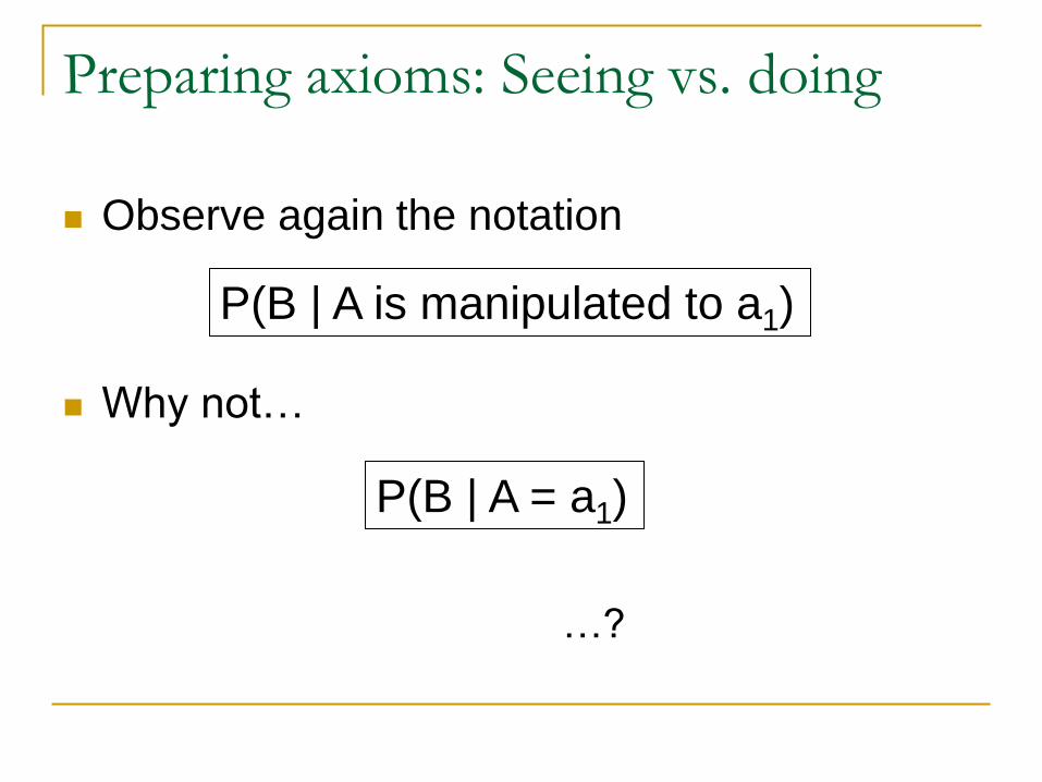
Observe again the notation
Why not…
P(B | A is manipulated to a1)
P(B | A = a1)
…?
Page 12
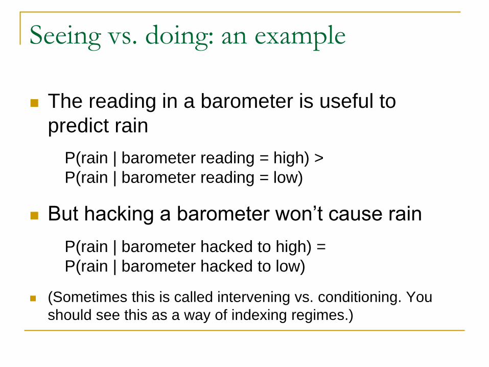
Seeing vs. doing: an example
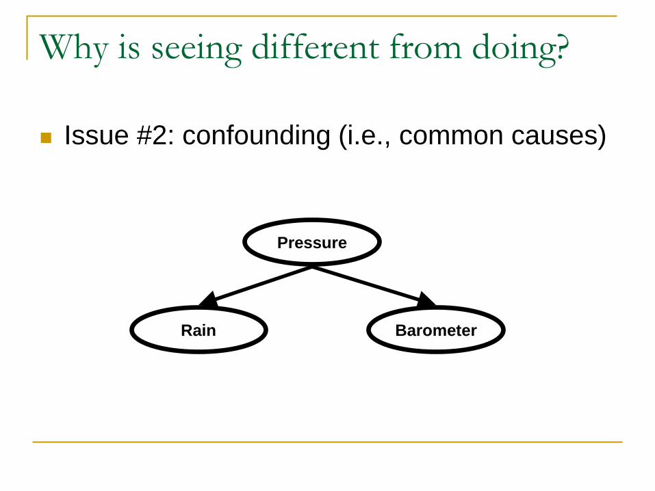
The reading in a barometer is useful to
predict rain
But hacking a barometer won’t cause rain
(Sometimes this is called intervening vs. conditioning. You
should see this as a way of indexing regimes.)
P(rain | barometer reading = high) >
P(rain | barometer reading = low)
P(rain | barometer hacked to high) =
P(rain | barometer hacked to low)
Page 13
Why is seeing different from doing?
Issue #1: directionality
Drinking
Car accidents
Page 14
Why is seeing different from doing?
Issue #2: confounding (i.e., common causes)
Pressure
Rain Barometer
Page 15
Why is seeing different from doing?
Most important lesson: unmeasured
confounding (i.e., hidden common causes) is
perhaps the most complicating factor of all
(but see also: measurement error and sampling selection bias)
Genotype
Smoking Lung cancer
Page 16
The do operator (Pearl’s notation)
A shorter notation
P(A | B = b): the probability of A being true given an observation of B = b
That is, no external intervention
This is sometimes called the distribution under the natural state of A
P(A | do(B = b)): the probability of A given an intervention that sets B to b
P(A | do(B)): some shorter notation for do(B) = true
Page 17
Different do’s
P(A | do(B), C)
Intervening on B, seeing C
P(A | do(B), do(C))
Multiple interventions
P(A | do(P(B) = P’))
A change on the distribution of B (not only a point
mass distribution)
Page 18
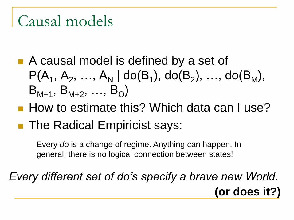
Causal models
A causal model is defined by a set of
P(A1, A2, …, AN | do(B1), do(B2), …, do(BM),
BM+1, BM+2, …, BO)
How to estimate this? Which data can I use?
The Radical Empiricist says:
Every do is a change of regime. Anything can happen. In
general, there is no logical connection between states!
Every different set of do’s specify a brave new World.
(or does it?)
Page 19
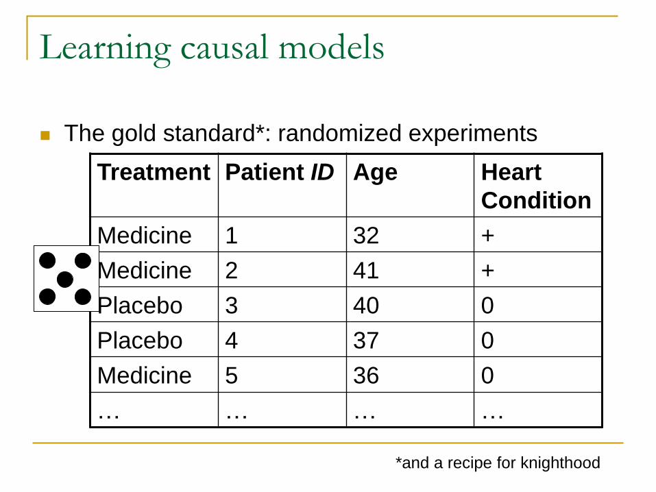
Learning causal models
The gold standard*: randomized experiments
Treatment Patient ID Age Heart
Condition
Medicine 1 32 +
Medicine 2 41 +
Placebo 3 40 0
Placebo 4 37 0
Medicine 5 36 0
… … … …
*and a recipe for knighthood
Page 20
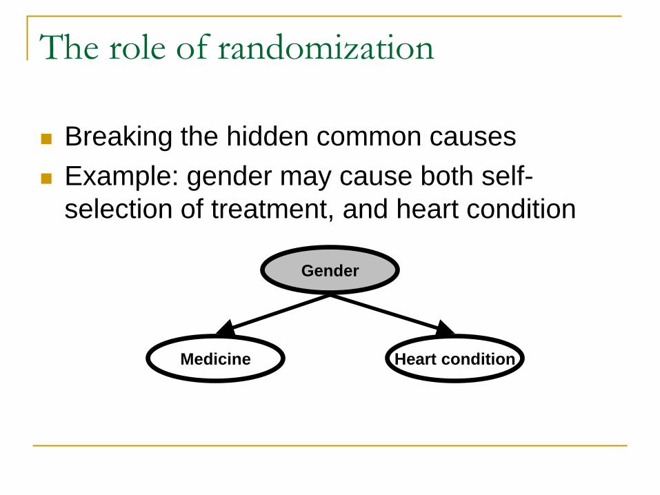
The role of randomization
Breaking the hidden common causes
Example: gender may cause both self-
selection of treatment, and heart condition
Gender
Medicine Heart condition
Page 21
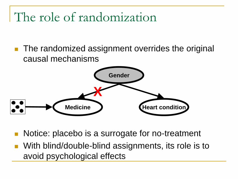
The role of randomization
The randomized assignment overrides the original
causal mechanisms
Notice: placebo is a surrogate for no-treatment
With blind/double-blind assignments, its role is to
avoid psychological effects
Gender
Medicine Heart condition
X
Page 22
Causal models
A causal model is defined by a set of
P(A1, A2, …, AN | do(B1), do(B2), …, do(BM),
BM+1, BM+2, …, BO)
Do I always have to perform an experiment?
Page 23
Observational studies
The art and science of inferring causation
without experiments
This can only be accomplished if extras
assumptions are added
Most notable case: inferring the link between
smoking and lung cancer
This tutorial will focus on observational
studies
Page 24
Observational studies
If you can do a randomized experiment, you
should do it
Observational studies have important roles,
though:
When experiments are impossible for
unethical/practical reasons
The case for smoking/lung cancer link
When there are many experiments to perform
A type of exploratory data analysis/active learning tool
E.g., biological systems
Page 25
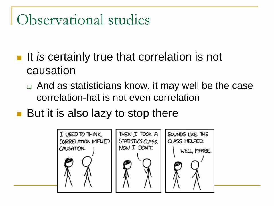
Observational studies
It is certainly true that correlation is not
causation
And as statisticians know, it may well be the case
correlation-hat is not even correlation
But it is also lazy to stop there
Page 26
Observational studies
Page 27
John Snow’ Soho
All image sources:
Wikipedia
Page 28
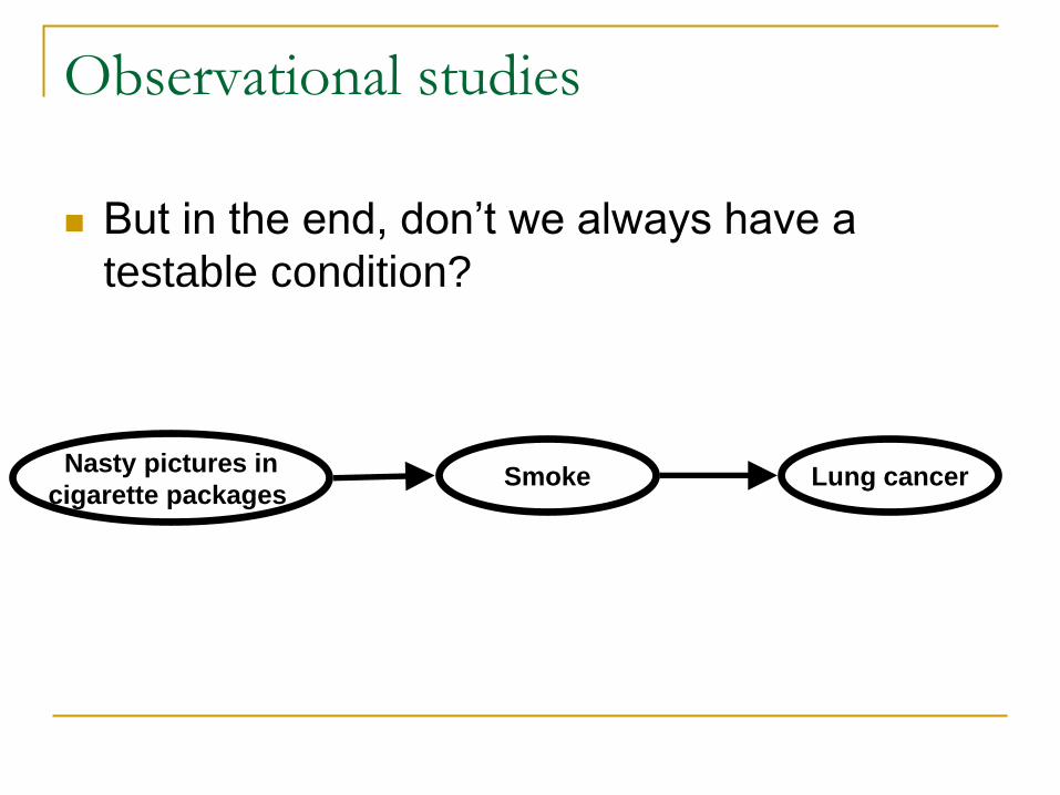
Observational studies
But in the end, don’t we always have a
testable condition?
Nasty pictures in
cigarette packages Lung cancer Smoke
Page 29
Observational studies
Appropriate interventions are much more
subtle than you might think…
Nasty pictures in
cigarette packages Smoke Lung cancer
“Gullibility trait”
expression level
Smoke Lung cancer | do(Smoke)
Page 30
(Sort of) Observational studies
Anna “likes” it Bob “likes” it
But I’m Facebook and I have 1 googol-
pounds of money for experiments. I’m
covered, right?
Page 31
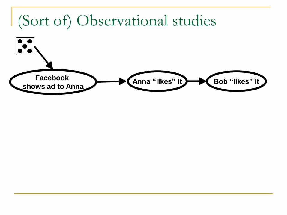
(Sort of) Observational studies
Facebook
shows ad to Anna Anna “likes” it Bob “likes” it
Page 32
(Sort of) Observational studies
Facebook
shows ad to Anna Anna “likes” it Bob “likes” it
Facebook
shows ad to Anna Anna “likes” it Bob “likes” it
Radio show advert
Page 33
(Sort of) Observational studies
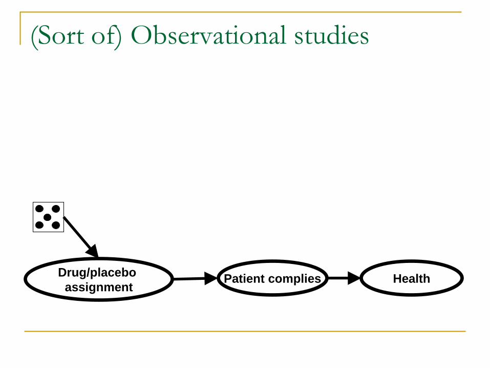
Drug/placebo
assignment Patient complies Health
Page 34
(Sort of) Observational studies
Drug/placebo
assignment Patient complies Health
Here be
dragons
Page 35
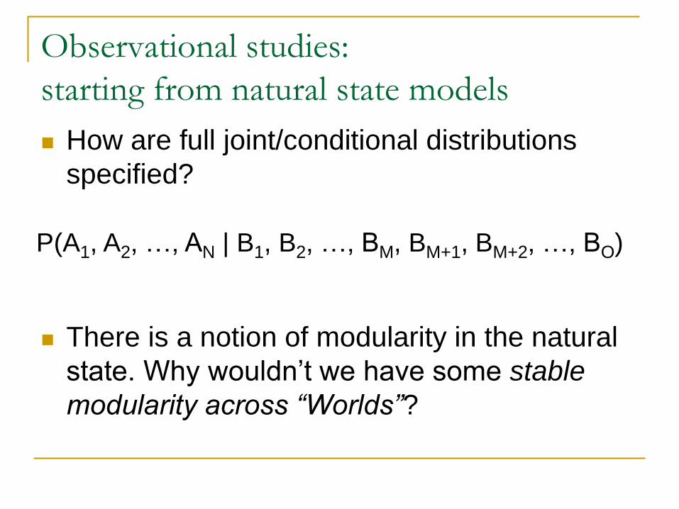
Observational studies:
starting from natural state models
How are full joint/conditional distributions
specified?
There is a notion of modularity in the natural
state. Why wouldn’t we have some stable
modularity across “Worlds”?
P(A1, A2, …, AN | B1, B2, …, BM, BM+1, BM+2, …, BO)
Page 36
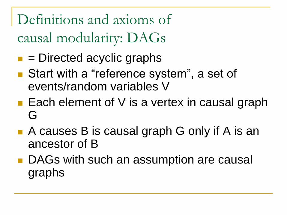
Definitions and axioms of
causal modularity: DAGs
= Directed acyclic graphs
Start with a “reference system”, a set of events/random variables V
Each element of V is a vertex in causal graph G
A causes B is causal graph G only if A is an ancestor of B
DAGs with such an assumption are causal graphs
Page 37
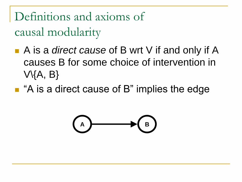
Definitions and axioms of
causal modularity
A is a direct cause of B wrt V if and only if A
causes B for some choice of intervention in
V\{A, B}
“A is a direct cause of B” implies the edge
A B
Page 38
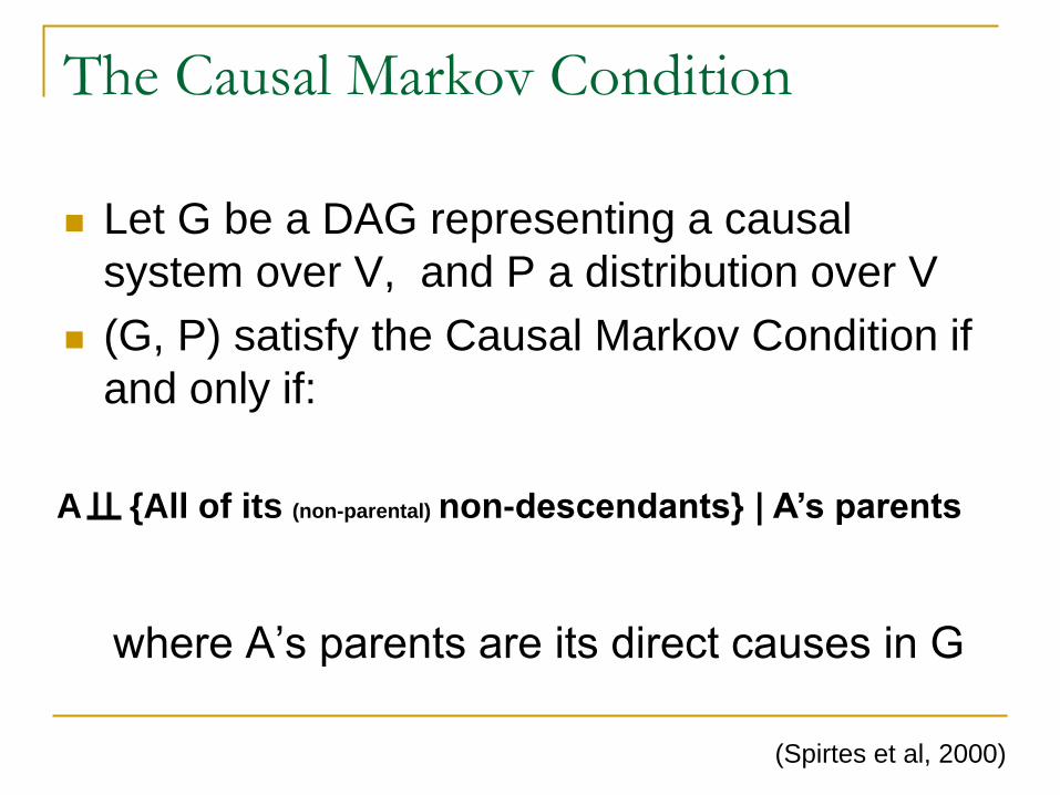
The Causal Markov Condition
Let G be a DAG representing a causal
system over V, and P a distribution over V
(G, P) satisfy the Causal Markov Condition if
and only if:
where A’s parents are its direct causes in G
A {All of its (non-parental) non-descendants} | A’s parents
(Spirtes et al, 2000)
Page 39
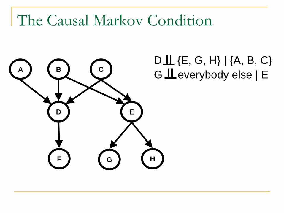
The Causal Markov Condition
D
F G H
A B C
E
D {E, G, H} | {A, B, C}
G everybody else | E
Page 40
Limitations of the Causal Markov
condition?
Sound Picture
TV switch
P(Picture | Switch) < P(Picture | Switch, Sound)
Where did the independence go?
Sound Picture
TV switch
Closed circuit
“The Interactive Fork”
(Spirtes et al, 2000)
Page 41
Causal models, revisited
Instead of an exhaustive “table of
interventional distributions”:
G = (V, E), a causal graph with vertices V and
edges E
P(), a probability over the “natural state” of V,
parameterized by
(G, ) is a causal model if pair
(G, P) satisfies the Causal Markov condition
We will show how to compute the effect of
interventions
Page 42
To summarize: what’s different?
As you probably know, DAG models can be
non-causal
What makes
causal?
A B
Answer: because I said so!
Page 43
To summarize
A causal graph is a way of encoding causal
assumptions
Graphical models allow for the evaluation of the
consequences of said assumptions
Typical criticism:
“this does not advance the ‘understanding’ of causality”
However, it is sufficient for predictions
And no useful non-equivalent alternatives are
offered
Page 44
Example of axioms in action:
Simpson’s paradox
(Pearl, 2000)
P(E | F, C) < P(E | F, C)
P(E | F, C) < P(E | F, C)
P(E | C) > P(E | C)
The “paradox”:
Which table to use?
(i.e., condition on gender or not?)
Page 45
To condition or not to condition:
some possible causal graphs
Page 46
Dissolving a “paradox” using the do
operator
Let our population have some subpopulations
Say, F and F
Let our treatment C not cause changes in the distribution of the subpopulations
P(F | do(C)) = P(F | do(C)) = P(F)
Then for outcome E it is impossible that we have, simultaneously,
P(E | do(C), F) < P(E | do(C), F)
P(E | do(C), F) < P(E | do(C), F)
P(E | do(C)) > P(E | do(C))
Page 48
Part II:
Predictions with observational data
Page 49
Goals and methods
Given: a causal graph, observational data
Task: estimate P(E | do(C))
Approach:
Perform a series of modifications on
P(E | do(C)), as allowed by the causal
assumptions, until no do operators appear
Estimate quantity using observational data
That is, reduce the causal query to a probabilistic
query
(Spirtes et al, 2000 – Chapter 7; Pearl, 2000 – Chapter 3)
Page 50
The trivial case
Graph:
A representation of a do(A) intervention
A B
A B T
Page 51
The trivial case
B is independent of T given A
P(B | do(A)) = P(B | A, T) = P(B | A)
Term on the right is identifiable from
observational data
do-free
That is, P(B | do(A)) can be estimated as
P(B | A)
Page 52
A less trivial case
Knowledge:
Query: P(B | do(A))
A B
F
Page 53
A less trivial case
With intervention
B and T are not independent given A
anymore…
A B
F
T
Page 54
A less trivial case
Solution: conditioning
Now, B is independent of T given A and F
A B
F
T
Page 55
A less trivial case
P(B | do(A)) = P(B | do(A), F)P(F | do(A)) + P(B | do(A), F)P(F | do(A)) = P(B | A, F, T)P(F) + P(B | A, F, T)P(F) = P(B | A, F)P(F) + P(B | A, F)P(F)
A B
F
T
“F-independent” intervention
Page 56
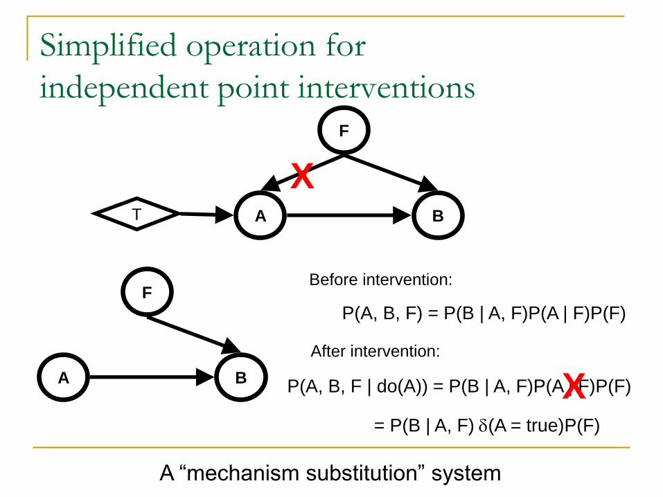
Simplified operation for
independent point interventions
A B
F
T
X
A B
F
P(A, B, F) = P(B | A, F)P(A | F)P(F)
Before intervention:
After intervention:
P(A, B, F | do(A)) = P(B | A, F)P(A | F)P(F) X = P(B | A, F)(A = true)P(F)
A “mechanism substitution” system
Page 57
Those “back-doors”…
Any common ancestor of A and B in the
graph is a confounder
Confounders originate “back-door” paths that
need to be blocked by conditioning
Page 58
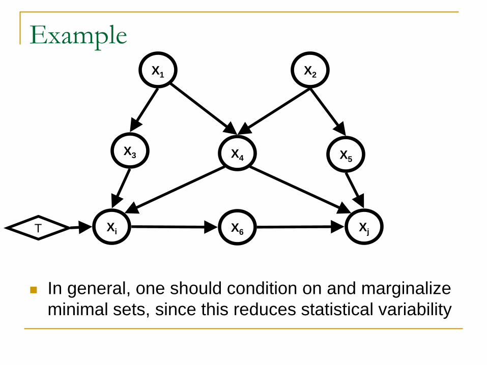
Example
In general, one should condition on and marginalize
minimal sets, since this reduces statistical variability
Xi X6 Xj
X3
X1
X4 X5
X2
T
Page 59
Unobserved confounding
If some variables are hidden, then there is no data for conditioning
Ultimately, some questions cannot be answered without extra assumptions
But there are other methods beside back-door adjustment
A B
U
Page 60
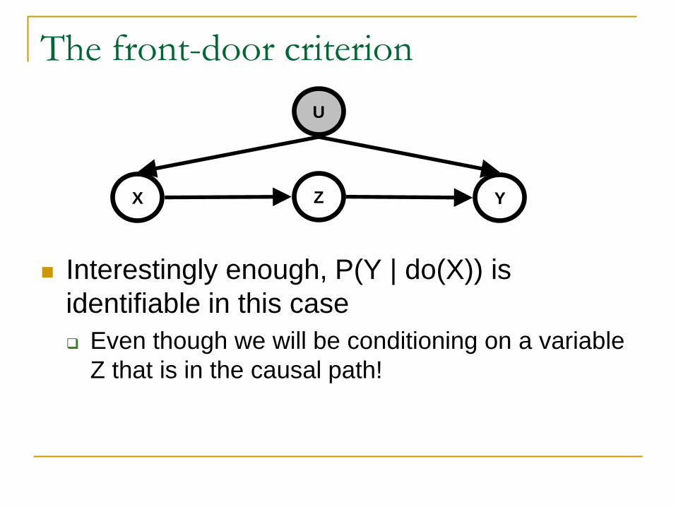
The front-door criterion
Interestingly enough, P(Y | do(X)) is
identifiable in this case
Even though we will be conditioning on a variable
Z that is in the causal path!
X Z
U
Y
Page 61
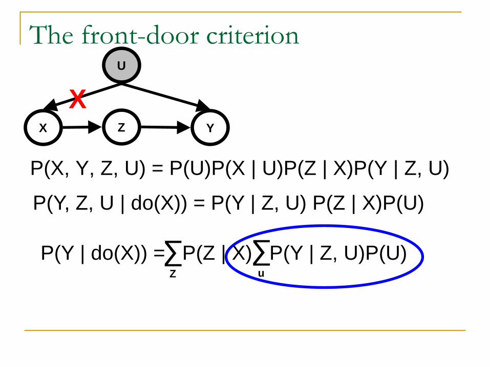
P(Y | do(X)) = P(Z | X) P(Y | Z, U)P(U)
∑ Z
∑ u
The front-door criterion
P(X, Y, Z, U) = P(U)P(X | U)P(Z | X)P(Y | Z, U)
X Z
U
Y
P(Y, Z, U | do(X)) = P(Y | Z, U) P(Z | X)P(U)
X
Page 62
The front-door criterion
X Z
U
Y
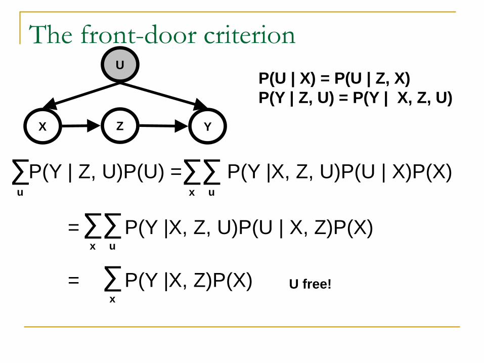
P(U | X) = P(U | Z, X)
P(Y | Z, U) = P(Y | X, Z, U)
P(Y | Z, U)P(U) = P(Y |X, Z, U)P(U | X)P(X)
∑ u
∑ x
∑ u
= P(Y |X, Z, U)P(U | X, Z)P(X)
∑ x
∑ u
= P(Y |X, Z)P(X)
∑ x
U free!
Page 63
A calculus of interventions
Back-door and front-door criteria combined
result in a set of reduction rules
Notation:
GX
X
X X
GX
X
X X
Page 64
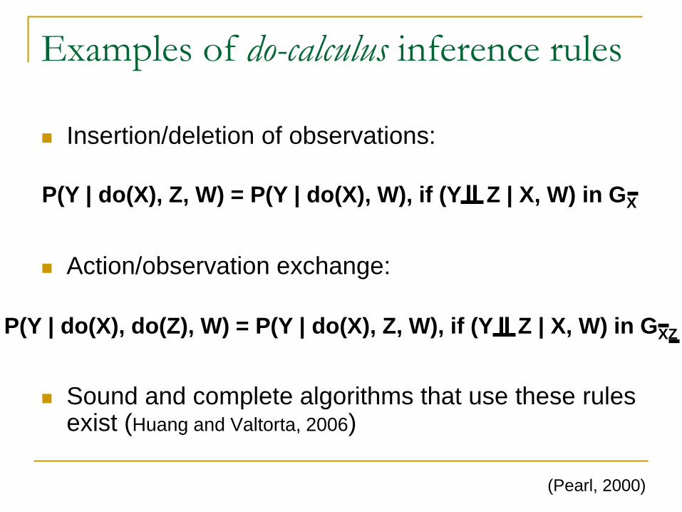
Examples of do-calculus inference rules
Insertion/deletion of observations:
Action/observation exchange:
Sound and complete algorithms that use these rules exist (Huang and Valtorta, 2006)
(Pearl, 2000)
P(Y | do(X), Z, W) = P(Y | do(X), W), if (Y Z | X, W) in GX
P(Y | do(X), do(Z), W) = P(Y | do(X), Z, W), if (Y Z | X, W) in GXZ
Page 65
A more complex example…
P(Y | do(X), do(Z2)) =
P(Y | Z1, do(X), do(Z2)) x
P(Z1 | do(X), do(Z2))
Y
Z1 Z2
X
∑ z1
= P(Y | Z1, X, Z2)P(Z1 | X) ∑ z1
(Now, Rule 2, for interchanging
observation/intervention)
Notice: P(Y | do(X)) is NOT identifiable!
Page 66
… and even more complex examples
Z1
X Z2
Z3
Y
P(Y | do(X)) is identifiable
(I’ll leave it as an exercise)
Page 67
Planning
Sequential decision problems:
More than one intervention, at different times
Intervention at one time depends on previous
interventions and outcomes
Example: sequential AIDS treatment (Robins,
1999)
PCP dose Pneumonia HIV load
AZT dose
T Will typically depend on
other parents
Page 68
Total and direct effects
A definition of causal effect: ACE
ACE(x, x’, Y) = E(Y | do(X = x’)) – E(Y | do(X = x))
Controlled direct effects in terms of do(.):
DEa(pcp1, pcp2, HIV) =
E(HIV | do(AZT) = a, do(PCP = pcp1))
– E(HIV | do(AZT) = a, do(PCP = pcp2))
PCP dose Pneumonia HIV load AZT dose
Page 69
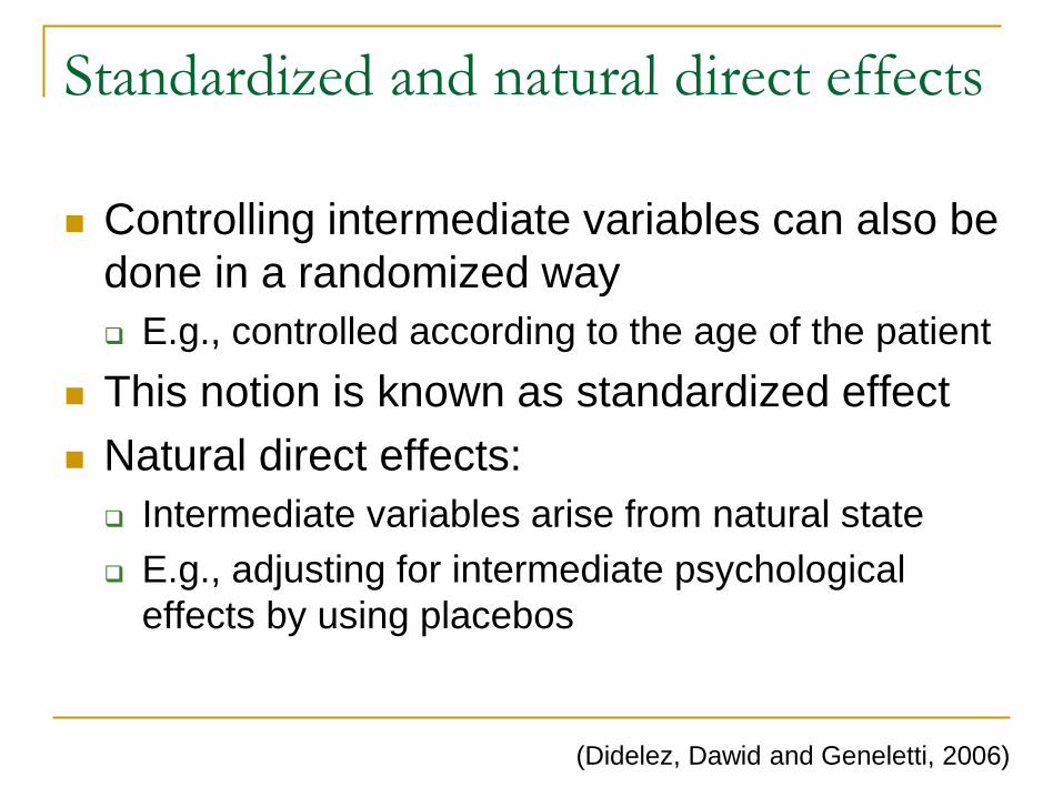
Standardized and natural direct effects
Controlling intermediate variables can also be
done in a randomized way
E.g., controlled according to the age of the patient
This notion is known as standardized effect
Natural direct effects:
Intermediate variables arise from natural state
E.g., adjusting for intermediate psychological
effects by using placebos
(Didelez, Dawid and Geneletti, 2006)
Page 70
Dealing with unidentifiability
We saw techniques that identify causal
effects, if possible
What if it is not possible?
The dreaded “bow-pattern”:
X Y
Page 71
Instrumental variables
One solution: explore parametric
assumptions and other variables
Classical case: the linear instrumental
variable
X Y Z
X = aZ + X
Y = bX + Y
X Y
a b
Page 72
Instrumental variables
Let Z be a standard Gaussian:
YZ = ab, xz = a
That is, b = YZ / XZ
Bounds can be generated for non-linear systems
Advertising: see my incoming NIPS paper for an example
and references
X Y Z
a b
Page 73
Bayesian analysis of confounding
Priors over confounding factors
Buyer Beware: priors have to have a
convincing empirical basis
not a small issue
Example: epidemiological studies of
occupational hazards
Are industrial sand workers more likely to suffer
from lung cancer?
Since if so, they should receive compensations
(Steenland and Greenland, 2004)
Page 74
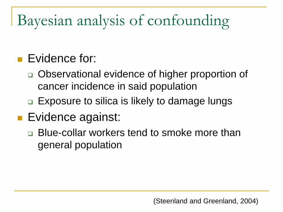
Bayesian analysis of confounding
Evidence for:
Observational evidence of higher proportion of
cancer incidence in said population
Exposure to silica is likely to damage lungs
Evidence against:
Blue-collar workers tend to smoke more than
general population
(Steenland and Greenland, 2004)
Page 75
Quantitative study
Sample of 4,626 U.S. workers, 1950s-1996
Smoking not recorded: becomes unmeasured
confounder
Prior: empirical priors pulled from population in
general
Assumes relations between subpopulations are
analogous
(Steenland and Greenland, 2004)
Occupation Lung cancer
Smoking
Page 76
Quantitative study
(Steenland and Greenland, 2004)
Page 77
Part III:
Learning causal structure
Page 78
From association to causation
We require a causal model to compute
predictions
Where do you get the model?
Standard answer: prior knowledge
Yet one of the goals is to use observational
data
Can observational data be used to infer a
causal model?
or at least parts of it?
Page 79
From association to causation
This will require going beyond the Causal
Markov condition…
independence in the causal graph
independence in probability
…into the Faithfulness Condition
independence in the causal graph
independence in probability
Notice: semiparametric constraints also
relevant, but not discussed here
(Spirtes et al., 2000; Pearl, 2000)
Page 80
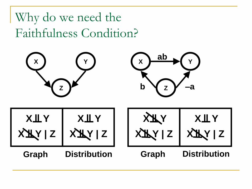
Why do we need the
Faithfulness Condition?
X Y
Z
X Y
Z
ab
–a b
X Y
X Y | Z
X Y
X Y | Z
X Y
X Y | Z
X Y
X Y | Z
Graph Distribution Graph Distribution
Page 81
Why would we accept the
Faithfulness Condition?
Many statisticians don’t
Putting the Radical Empiricist hat: “anything goes”
Yet many of these don’t see much of a problem
with the Causal Markov condition
But then unfaithful distributions are equivalent
to accidental cancellations between paths
How likely is that?
Page 82
Arguments for Faithfulness
The measure-theoretical argument :
probability one in multinomial and Gaussian
families (Spirtes et al., 2000)
The experimental analysis argument:
Not spared of faithfulness issues (in a less
dramatic sense)
How often do you see zero-effect strong causes?
Coffee-Cola Heart Attack
Exercise + -
+
Page 83
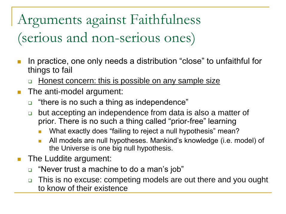
Arguments against Faithfulness
(serious and non-serious ones)
In practice, one only needs a distribution “close” to unfaithful for things to fail
Honest concern: this is possible on any sample size
The anti-model argument:
“there is no such a thing as independence”
but accepting an independence from data is also a matter of prior. There is no such a thing called “prior-free” learning
What exactly does “failing to reject a null hypothesis” mean?
All models are null hypotheses. Mankind’s knowledge (i.e. model) of the Universe is one big null hypothesis.
The Luddite argument:
“Never trust a machine to do a man’s job”
This is no excuse: competing models are out there and you ought to know of their existence
Page 84
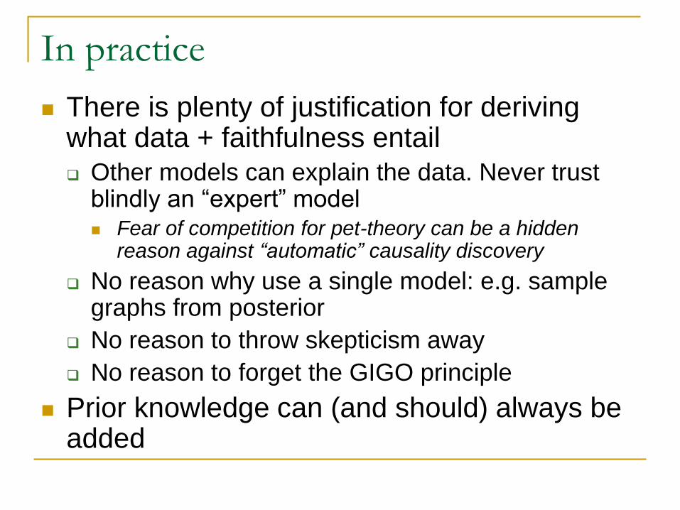
In practice
There is plenty of justification for deriving what data + faithfulness entail
Other models can explain the data. Never trust blindly an “expert” model Fear of competition for pet-theory can be a hidden
reason against “automatic” causality discovery
No reason why use a single model: e.g. sample graphs from posterior
No reason to throw skepticism away
No reason to forget the GIGO principle
Prior knowledge can (and should) always be added
Page 85
X Z | Y
Algorithms: principles
Markov equivalence classes:
Limitations on what can be identifiable with
conditional independence constraints
X Y Z
X Y Z
X Y Z
Page 86
Algorithms: principles
The goal:
Learn a Markov equivalence class
Some predictions still identifiable (Spirtes et al.,
2000)
A few pieces of prior knowledge (e.g., time order)
can greatly improve identifiability results
Provides a roadmap for experimental analysis
Side note: Markov equivalence class is not the
only one
Page 87
Initial case: no hidden common causes
Little motivation for that, but easier to explain
“Pattern”: a graphical representation of
equivalence classes
X Y K
Z
Page 88
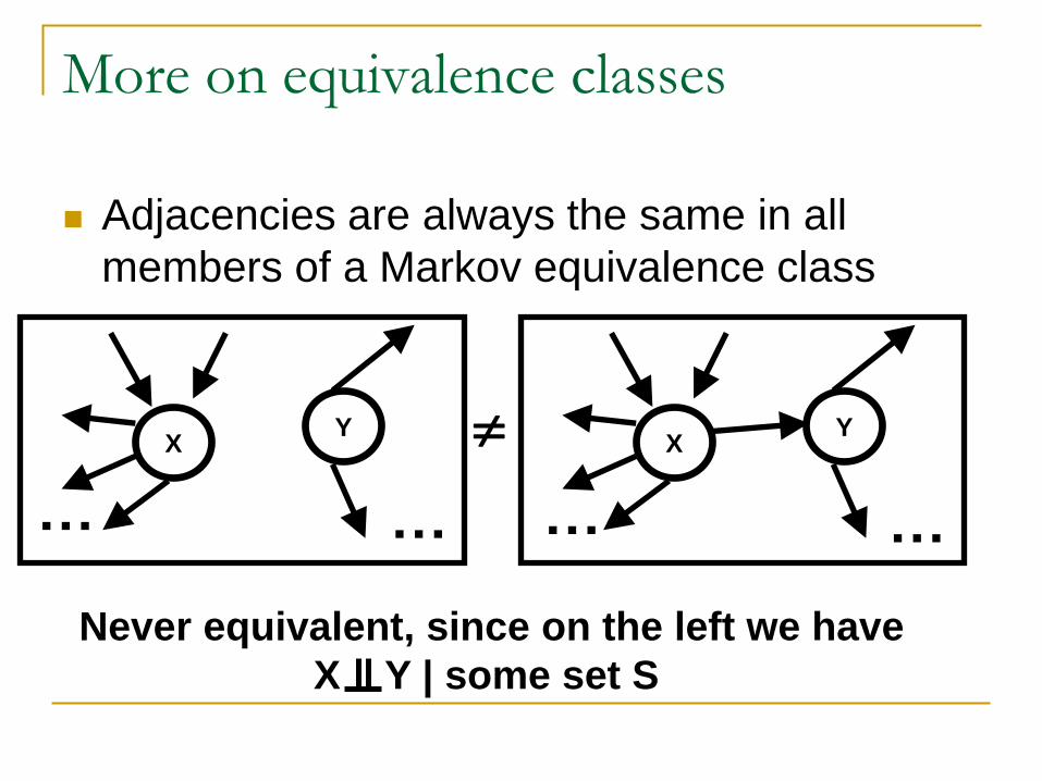
More on equivalence classes
Adjacencies are always the same in all
members of a Markov equivalence class
X
Y X
Y
Never equivalent, since on the left we have
X Y | some set S
… … … …
Page 89
More on equivalence classes
Unshielded colliders: always identifiable
X Y
Z
Unshielded collider Not a unshielded collider
T U
V
X Y
Z
T U
V
Page 90
More on equivalence classes
“Propagating” unshielded colliders
X Y
Z
W
X Y
Z
W
Why? Different unshielded colliders
Markov
Page 91
Algorithms: two main families
Piecewise (constraint-satisfaction) algorithms
Evaluate each conditional independence
statement individually, put pieces together
Global (score-based) algorithms
Evaluate “all” models that entail different
conditional independencies, pick the “best”
“Best” in a statistical sense
“All” in a computationally convenient sense
Two endpoints of a same continuum
Page 92
A constraint-satisfaction algorithm:
the PC algorithm
Start by testing marginal independencies
Is X1 independent of X2?
Is X1 independent of X3?
…
Is XN – 1 independent of XN?
Such tests are usually frequentist hypothesis
tests of independence
Not essential: could be Bayes factors too
Page 93
The PC algorithm
Next step: conditional independencies tests of “size” 1
Is X1 independent of X2 given X3?
Is X1 independent of X2 given X4?
…
(In practice only a few of these tests are performed, as we will illustrate)
Continue then with tests of size 2, 3, … etc. until no tests of a given size pass
Orient edges according to which tests passed
Page 94
The PC algorithm: illustration
Assume the model on the
left is the real model
Observable: samples
from the observational
distribution
Goal: recover the pattern
(equivalence class
representation)
X Y
Z
W
T
Page 95
PC, Step 1: find adjacencies X Y
Z
W
T
X Y
Z
W
T
Start
X Y
Z
W
T
Size 1
X Y
Z
W
T
Size 2
Page 96
PC, Step 2: collider orientation
X and Y are independent given T
Therefore, X T Y is not possible
At the same time, X Z Y
X Z Y
X Z Y
are not possible, or otherwise X and Y would not be independent given T
Therefore, it has to be the case that X Z Y
Check all unshielded triples
X Y
Z
W
T
Page 97
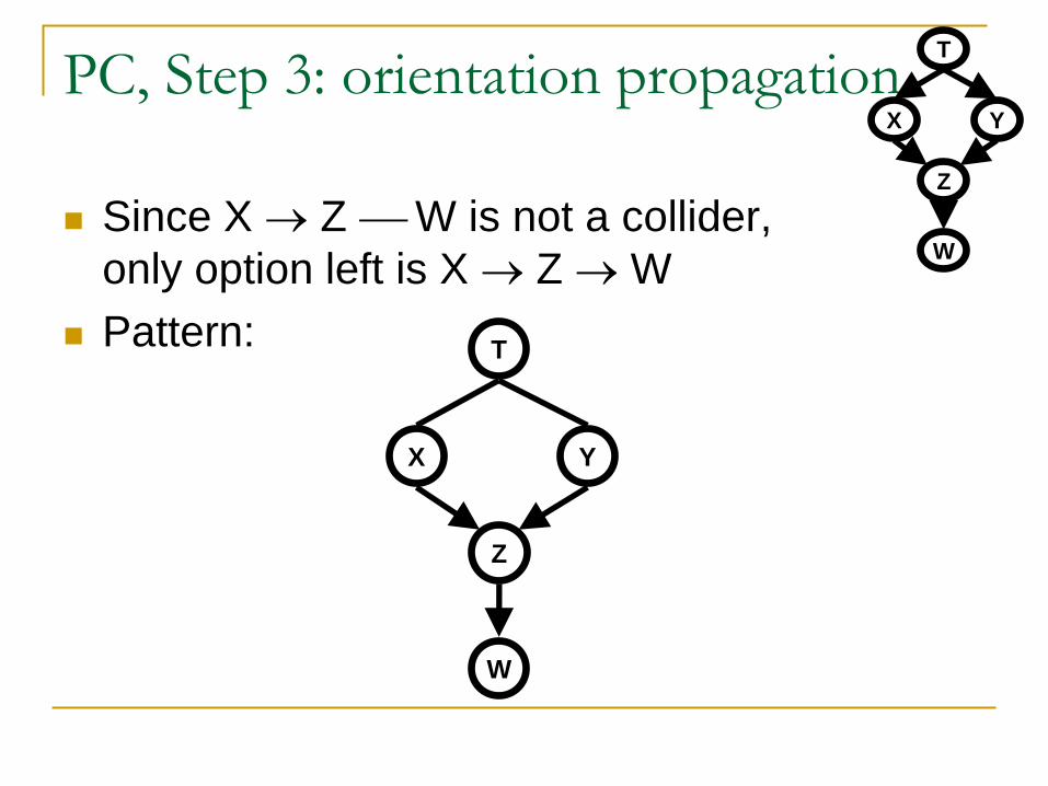
PC, Step 3: orientation propagation
Since X Z W is not a collider,
only option left is X Z W
Pattern:
X Y
Z
W
T
X Y
Z
W
T
Page 98
Advantages and shortcomings
Fast
Only submodels are compared
Prunes search space very effectively
Consistent
On the limit on infinite data
But brittle
Only submodels are compared: very prone to statistical
mistakes
Doesn’t enforce global constraint of acyclicity
Might generate graphs with cycles
(which is actually good and bad)
Page 99
Simple application: evolutionary biology
Using a variation of PC + bootstrapping in
biological domain:
(Shipley, 1999)
Seed
weight
Fruit
diameter
Canopy
projection
Number
fruit
Number
seeds
dispersed
Seed
weight
Fruit
diameter
Canopy
projection
Number
fruit
Number
seeds
dispersed
Page 100
Simple application: botanic
Very small sample size (35):
(Shipley, 1999)
Specific
leaf mass
Leaf
nitrogen
Stomatal
conductance
Internal
CO2
Photosynthesis
Page 101
Simple application: botanic
Forcing blue edge by background knowledge
Specific
leaf mass
Leaf
nitrogen
Stomatal
conductance
Internal
CO2
Photosynthesis
(Shipley, 1999)
Page 102
Global methods for structure learning
Compares whole graphs against whole graphs
Typical comparison criterion (score function): posterior distribution
P(G1 | Data) > P(G2 | Data), or the opposite?
Classical algorithms: greedy search
Compares nested models: one model differs from the other by an adjacency
Some algorithms search over DAGs, others over patterns
Page 103
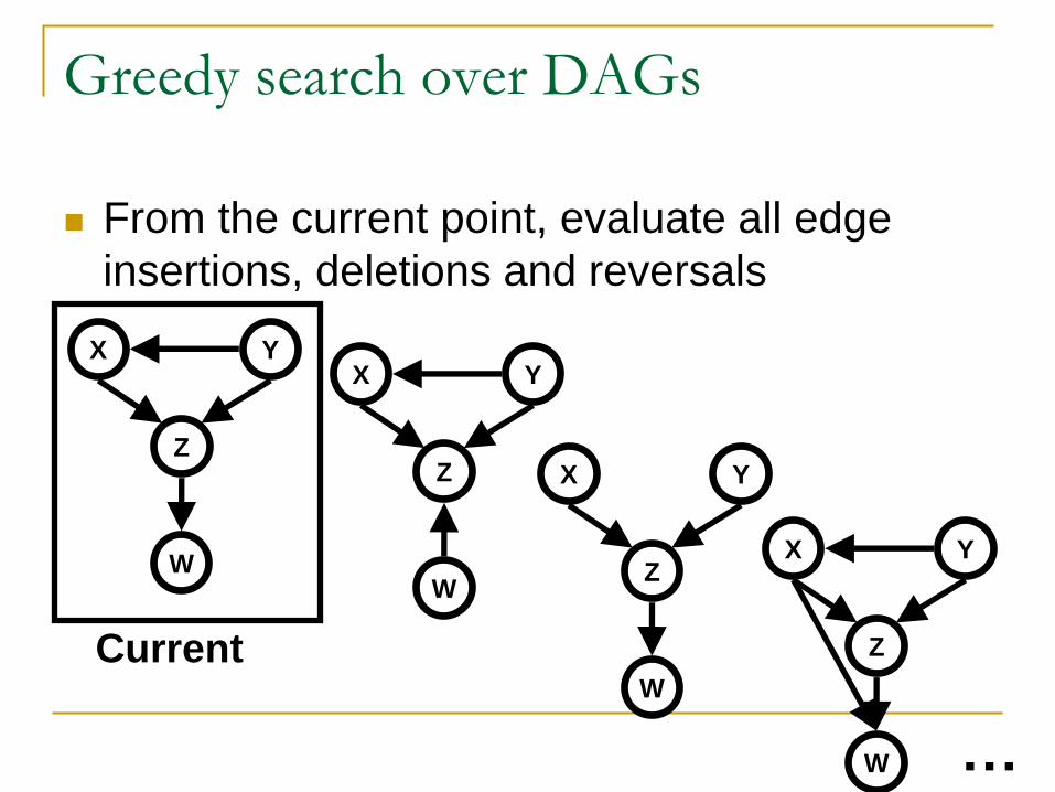
Greedy search over DAGs
From the current point, evaluate all edge
insertions, deletions and reversals
X Y
Z
W
X Y
Z
W
X Y
Z
W
X Y
Z
W …
Current
Page 104
Greedy search over patterns
Evaluate all patterns that differ by one
adjacency from the current one
Unlike DAG-search, consistent (starting point
doesn’t matter)
But the problem is NP-hard…
Y
X1 X2 Xk X …
Y
X1 X2 Xk X …
new 2k different patterns…
Page 105
Combining observational and
experimental data
Model selection scores are usually
decomposable:
Remember DAG factorization:
Score factorization (such as log-posterior):
i P(Xi | Parents(Xi))
Score(G) = ∑i S(Xi, Parents(Xi))
(Cooper and Yoo, 1999)
Page 106
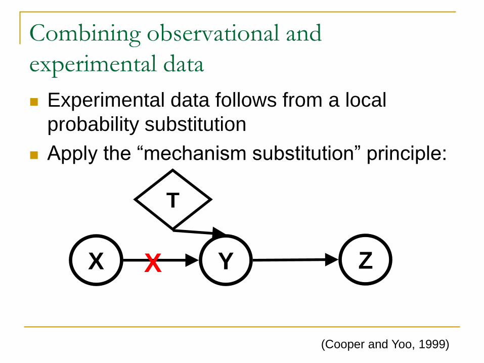
Combining observational and
experimental data
Experimental data follows from a local
probability substitution
Apply the “mechanism substitution” principle:
(Cooper and Yoo, 1999)
X Y Z
T
X
Page 107
Combining observational and
experimental data
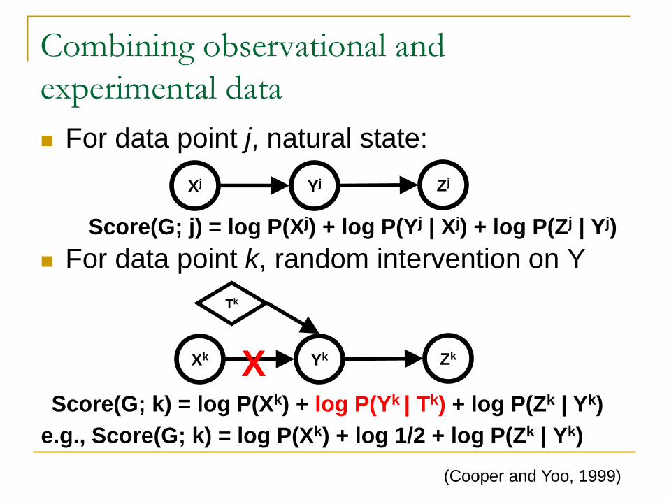
For data point j, natural state:
For data point k, random intervention on Y
Xj Yj Zj
Score(G; j) = log P(Xj) + log P(Yj | Xj) + log P(Zj | Yj)
Xk Yk Zk
Tk
Score(G; k) = log P(Xk) + log P(Yk | Tk) + log P(Zk | Yk)
e.g., Score(G; k) = log P(Xk) + log 1/2 + log P(Zk | Yk)
X
(Cooper and Yoo, 1999)
Page 108
Computing structure posteriors
Notice: greedy algorithms typically return the
maximum a posteriori (MAP) graph
Or some local maxima of the posterior
Posterior distributions
Practical impossibility for whole graphs
MCMC methods should be seeing as stochastic search
methods, mixing by the end of the universe
Still: 2 graphs are more useful than 1
Doable for (really) small subgraphs: edges, short
paths (Friedman and Koller, 2000)
Page 109
Computing structure posteriors:
a practical approach
Generate a few high probability graphs
E.g.: use (stochastic) beam-search instead of
greedy search
Compute and plot marginal edge posteriors
X
Y
Z W
Page 110
A word of warning
Uniform consistency: impossible with faithfulness
only (Robins et al., 2003)
Considering the case with unmeasured confounding
Rigorously speaking, standard Bayesian posteriors
reflect independence models, not causal models
There is an implicit assumption that the distribution
is not “close” to unfaithfulness
A lot of work has yet to be done to formalize this (Zhang
and Spirtes, 2003)
Page 111
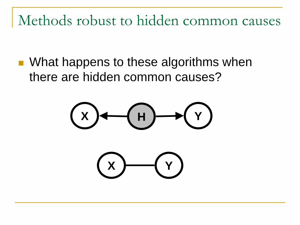
Methods robust to hidden common causes
What happens to these algorithms when
there are hidden common causes?
X Y H
X Y
Page 112
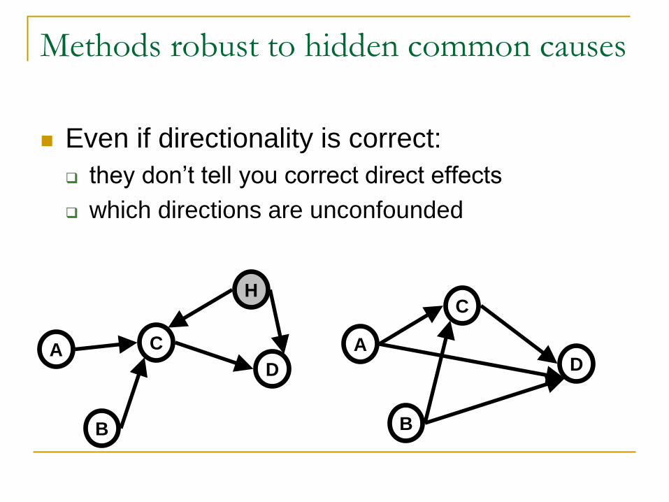
Methods robust to hidden common causes
Even if directionality is correct:
they don’t tell you correct direct effects
which directions are unconfounded
A
B
C
H
D
A
B
C
D
Page 113
Partial ancestral graphs (PAGs)
New representation of equivalence classes
(Spirtes et al., 2000)
Smoking
Income
Parent’s
smoking habits
Cilia
damage
Heart
disease
Lung
capacity
Breathing
dysfunction
Pollution Genotype
Page 114
Partial ancestral graphs (PAGs)
Type of edge:
Smoking
Income
Parent’s
smoking habits
Cilia
damage
Heart
disease
Lung
capacity
Breathing
dysfunction
Page 115
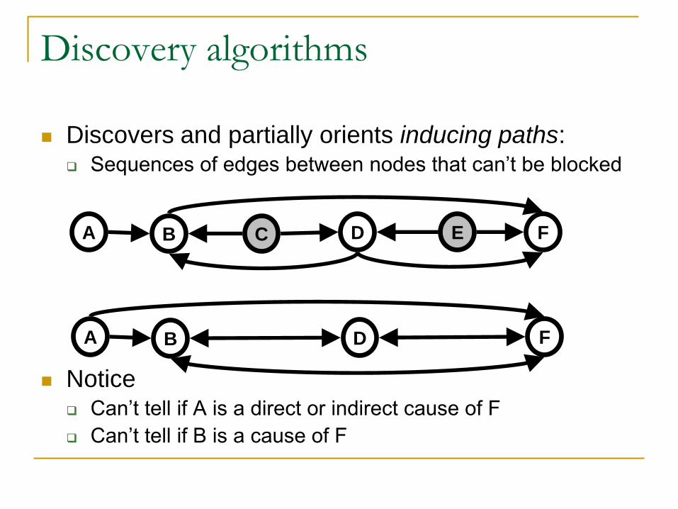
Discovery algorithms
Discovers and partially orients inducing paths: Sequences of edges between nodes that can’t be blocked
Notice Can’t tell if A is a direct or indirect cause of F
Can’t tell if B is a cause of F
A B C D E F
A B F D
Page 116
Algorithms
The “Fast” Causal Inference algorithm (FCI,
Spirtes et al., 2000):
“Fast” because it has a clever way of avoiding
exhaustive search (e.g., as in Pearl, 2000)
Sound and complete algorithms are fairly
recent: Zhang, 2005
Bayesian algorithms are largely
underdeveloped
Discrete model parameterization still a challenge
Page 118
Summary and other practical issues
There is no magic:
It’s assumptions + data + inference systems
Emphasis on assumptions
Still not many empirical studies
Requires expertise, ultimately requires
experiments for validation
Lots of work in fixed back-door designs
Graphical models not that useful (more so in longitudinal
studies)
Page 119
The future
Biological systems might be a great domain
That’s how it all started after all (Wright, 1921)
High-dimensional: make default back-door
adjustments dull
Lots of direct and indirect effects of interest
Domains of testable assumptions
Observational studies with graphical models can be a
great aid for experimental design
But beware of all sampling issues: measurement
error, small samples, dynamical systems, etc.
Page 120
What I haven’t talked about
Dynamical systems (“continuous-time” models)
Other models for (Bayesian) analysis of confounding Structural equations, mixed graphs et al.
Potential outcomes (Rosenbaum, 2002)
Detailed discovery algorithms Including latent variable models/non-independence
constraints
Active learning
Measurement error, sampling selection bias
Lack of overlap under conditioning
Formalizing non-ideal interventions Non-compliance, etc.
Page 122
Textbooks
Glymour, C. and Cooper, G. (1999). Computation, Causation and Discovery. MIT Press.
Pearl, J. (2000). Causality. Cambridge University Press.
Rosenbaum, P. (2002). Observational Studies. Springer.
Spirtes, P, Glymour, C. and Scheines, R. (2000). Causation, Prediction and Search. MIT Press.
Page 123
Other references
Brito, C. and Pearl, J. (2002) “Generalized instrumental variables.” UAI 2002
Cooper, G. and Yoo, C. (1999). “Causal inference from a mixture of experimental and observational data”. UAI 1999.
Robins, J. (1999). “Testing and estimation of direct effects by reparameterizing directed acyclic graphs with structural nested models.” In Computation, Causation and Discovery.
Robins, J., Scheines, R., Spirtes, P. and Wasserman, L. (2003). “Uniform convergence in causal inference.” Biometrika.
Shipley, B. (1999). “Exploring hypothesis space: examples from organismal biology”. Computation, Causation and Discovery, MIT Press.
Steenland, K. and Greenland, S. (2004). “Monte Carlo sensitivity analysis and Bayesian analysis of smoking as an unmeasured confounder in a study of silica and lung cancer”. American Journal of Epidemiology 160 (4).
Wright, S. (1921). “Cause and correlation.” Journal of Agricultural Research
Huang, Y. and Valtorta, M. (2006). "Identifiability in Causal Bayesian Networks: A Sound and Complete Algorithm." AAAI-06.
Zhang, J. and Spirtes, P. (2003). “Strong Faithfulness and Uniform Consistency in Causal Inference”. UAI 2003.
Zhang, J. (2005). PhD Thesis, Department of Philosophy, Carnegie Mellon University.
Page 124
To know more
A short article by me:
http://www.homepages.ucl.ac.uk/~ucgtrbd/papers/cau
sality.pdf
Hernan and Robins’ incoming textbook
http://www.hsph.harvard.edu/miguel-hernan/causal-
inference-book/
Pearl’s “Causality”
Spirtes/Glymour/Scheine’s “Causation,
Prediction and Search”
Morgan and Winship’s “Counterfactuals and
Causal Inference” (2nd edition out this weekend)