Causal Inference in Repeated Observational Studies: A Case Study of eBay Product Releases Vadim von Brzeski eBay Inc. and University of California, Santa Cruz Matt Taddy Booth School of Business, University of Chicago David Draper University of California, Santa Cruz Abstract Causal inference in observational studies is notoriously difficult, due to the fact that the experimenter is not in charge of the treatment assignment mechanism. Many potential con- founding factors (PCFs) exist in such a scenario, and if one seeks to estimate the causal effect of the treatment on a response, one needs to control for such factors. Identifying all relevant PCFs may be difficult (or impossible) given a single observational study. Instead, we argue that if one can observe a sequence of similar treatments over the course of a lengthy time period, one can identify patterns of behavior in the experimental subjects that are correlated with the response of interest and control for those patterns directly. Specifically, in our case-study we find and control for an early-adopter effect : the scenario in which the magnitude of the response is highly correlated with how quickly one adopts a treatment after its release. We provide a flexible hierarchical Bayesian framework that controls for such early-adopter effects in the analysis of the effects of multiple sequential treatments. The methods are presented and evaluated in the context of a detailed case-study involving product updates (newer versions of the same product) from eBay, Inc. The users in our study upgrade (or not) to a new version of the product at their own volition and timing. Our response variable is a measure of user actions, and we study the behavior of a large set of users (n = 10.5 million) in a targeted subset of eBay categories over a period of one year. We find that (a) naive causal estimates are hugely misleading and (b) our method, which is relatively insensitive to modeling assumptions and exhibits good out-of-sample predictive validation, yields sensible causal estimates that offer eBay a stable basis for decision-making. 1 Introduction Causal inference is a complex problem with a long history in statistics. Its general setup is as follows: given an observable response Y , a measurable treatment Z , a set of n subjects i =1,...,n, partitioned into distinct treatment (T ) and control (C ) groups, how much of the observed response was caused by the treatment? In the case of binary treatments, the potential outcomes approach (Neyman, 1923; Rubin, 1974) defines for each subject i two potential outcomes: the response of the subject under treatment Y i (Z i = 1) ≡ Y i (1), and the response of the subject under no-treatment (control) Y i (Z i = 0) ≡ Y i (0). However, for any individual subject i, we cannot observe both outcomes Y i (0) and Y i (1), hence the designation potential outcomes. Therefore, the fundamental 1 arXiv:1509.03940v1 [stat.AP] 14 Sep 2015
Transcript
Causal Inference in Repeated Observational Studies:
A Case Study of eBay Product Releases
Vadim von BrzeskieBay Inc. and University of California, Santa Cruz
Matt TaddyBooth School of Business, University of Chicago
David DraperUniversity of California, Santa Cruz
Abstract
Causal inference in observational studies is notoriously difficult, due to the fact that theexperimenter is not in charge of the treatment assignment mechanism. Many potential con-founding factors (PCFs) exist in such a scenario, and if one seeks to estimate the causal effectof the treatment on a response, one needs to control for such factors. Identifying all relevantPCFs may be difficult (or impossible) given a single observational study. Instead, we argue thatif one can observe a sequence of similar treatments over the course of a lengthy time period,one can identify patterns of behavior in the experimental subjects that are correlated with theresponse of interest and control for those patterns directly. Specifically, in our case-study wefind and control for an early-adopter effect : the scenario in which the magnitude of the responseis highly correlated with how quickly one adopts a treatment after its release.
We provide a flexible hierarchical Bayesian framework that controls for such early-adoptereffects in the analysis of the effects of multiple sequential treatments. The methods are presentedand evaluated in the context of a detailed case-study involving product updates (newer versionsof the same product) from eBay, Inc. The users in our study upgrade (or not) to a new versionof the product at their own volition and timing. Our response variable is a measure of useractions, and we study the behavior of a large set of users (n = 10.5 million) in a targetedsubset of eBay categories over a period of one year. We find that (a) naive causal estimates arehugely misleading and (b) our method, which is relatively insensitive to modeling assumptionsand exhibits good out-of-sample predictive validation, yields sensible causal estimates that offereBay a stable basis for decision-making.
1 Introduction
Causal inference is a complex problem with a long history in statistics. Its general setup is as
follows: given an observable response Y , a measurable treatment Z, a set of n subjects i = 1, . . . , n,
partitioned into distinct treatment (T ) and control (C) groups, how much of the observed response
was caused by the treatment? In the case of binary treatments, the potential outcomes approach
(Neyman, 1923; Rubin, 1974) defines for each subject i two potential outcomes: the response of the
subject under treatment Yi(Zi = 1) ≡ Yi(1), and the response of the subject under no-treatment
(control) Yi(Zi = 0) ≡ Yi(0). However, for any individual subject i, we cannot observe both
outcomes Yi(0) and Yi(1), hence the designation potential outcomes. Therefore, the fundamental
1
arX
iv:1
509.
0394
0v1
[st
at.A
P] 1
4 Se
p 20
15
problem of causal inference (Holland, 1986) is that to estimate the causal effect of a treatment, we
need to compare the two potential outcomes for each individual, namely [Yi(1)−Yi(0)], but we get
to observe only one of those quantities: either Yi(1) or Yi(0).
This task is further complicated in observational studies. Unlike randomized controlled trials
(Fisher, 1935), observational studies are characterized by the fact that the experimenter is not in
charge of the treatment assignment mechanism. A treatment event occurs at some point in time,
and data are collected on subjects before and after the treatment. Such a scenario makes it quite
likely that many potential confounding factors (PCFs) exist. PCFs are attributes of the subjects
(usually covariates) that are correlated with both the treatment assignment and the response, and
their existence leads to biased estimates of the causal effect unless they are adjusted/controlled for
in some way. Thus, in addition to modeling potential outcomes, causal inference in observational
studies requires the discovery of all PCFs that could have a bearing on valid estimation of the
causal effect.
Without loss of generality, let us imagine an observational study in which the response is some
measure of user activity (e.g., miles jogged, items bought, ads clicked), and where the availability of
a treatment is announced at some point in time. Users take advantage (or not) of the treatment at
their own volition over the subsequent days or weeks, and the response of each user is recorded over
time. Furthermore, suppose that (a) the majority of users who adopt the treatment at all do so
in a relatively short time period after its release, and (b) those users who are the earliest adopters
exhibit a higher average response compared to those who wait longer to try the treatment. In other
words, the waiting time to adopt the treatment is (negatively) correlated with the treatment and
the response, making it a PCF. We refer to this situation as the early-adopter effect : the overall
response is a (confounded) combination of the actual effect of the treatment and the effects of
characteristics associated with being an early adopter.
Situations where the early-adopter effect occurs arise with some frequency. For example, suppose
that a new diet and exercise plan is offered to the general public for free by a public-health agency.
It is a well-known fact in public health that, ironically, those who voluntarily adopt measures to
improve their health are precisely the people who need such measures the least, namely people
who are already health conscious. Comparing the health status, (say) six months after the plan
is offered, of those who chose to use it and those who did not will confound the effect of the plan
2
with the early-adopter effect.
This brings us to the major contribution of this paper. We demonstrate that in observational
studies where the early-adopter effect exists, it is difficult to obtain a reasonable estimate of the
treatment effect (on the treated) when one only considers a single treatment event. However,
we also show that the task is made considerably easier when one studies a sequence of similar
treatments over an extended period of time. In the single treatment event scenario, one’s only
option is to discover (typically static) user attributes that control for the early-adopter effect; in
other words, what is it about a user that makes him or her an early adopter? This may be a
difficult or impossible task if little or no data (e.g., demographic information) is available on the
users. On the other hand, given a sequence of similar treatments, the problem is greatly simplified
if we assume that the (unknown) early-adopter behavior is relatively consistent from one treatment
event to the next. In such a scenario, we do not need to know the true characteristics (true PCFs)
that make a user an early adopter. Instead, we simply include a set of (indicator) covariates that
encode a user’s waiting time into our models, and thus account for the early-adopter portion of
the total response, leading to a less biased estimate of the treatment effect. Given a sequence of K
treatments T1, . . . , TK , our approach makes the following two assumptions (which can be verified
by exploratory data analysis; see below):
• Early Adopter Effect: The average response per user subsequent to a treatment release
should follow a similar decaying pattern regardless of the particular treatment. If this is not
the case, the early-adopter effect may not exist at all. In one extreme scenario, we can imagine
the early-adopter effect for some treatments, and a late-adopter effect for other treatments
in which the average response shows an increasing pattern following its release. In such a
scenario, we would need to consider including second-order interactions into our models to
account for this.
• Identifiability: The users’ treatment adoption pattern (i.e., the specific timing with which
each user adopts a new treatment after its availability) should differ appreciably between
treatments. This allows us to have an identifiable model. In the extreme scenario, if each
treatment shows the exact same pattern of adoption across all users, we will have collinear
columns in our design matrix, resulting in a non-identifiable model. We return to this subject
in Section 4.
3
The remainder of the paper is organized as follows. In Section 2, we review the standard estimators
of treatment effects found in the observational-studies literature and describe the estimator we will
be using in our work. We also describe the exact nature of the causal inference problem at eBay.
effect estimates) are given in Section 4. We describe our model validation approach in Section 5,
where we check our assumptions and investigate the out-of-sample performance of our models. We
conclude in Section 6 with a summary of our major results.
2 Problem Statement and Definitions
2.1 Case Study: eBay Product Releases
Our case study deals with a sequence of observational studies at eBay Inc., in which analysts
attempted to infer the causal effect of new versions (releases) of a specific software product, hence-
forth referred to as the Product, on aggregate User Actions with said Product (the true response
and the true product are not disclosed for confidentiality reasons).
The exact nature of the Product is not important; however, it possesses a number of characteristics
that are relevant to our study. First, newer versions (upgrades) of the Product are released on a
semi-regular basis, with releases happening on the order of 6− 12 weeks apart on average. Second,
once a new version of the Product is released and becomes available to the general public, users
adopt (upgrade to) the new version at their own volition and timing. The new version of the
Product is not an en masse replacement of the previous version; instead, users choose to upgrade
to it or not. Some users upgrade immediately when (or shortly after) the version becomes available:
we will refer to these users as early adopters; some users never upgrade and continue to use the
same version of the Product throughout our study. This rolling treatment setting with user Product
choice is precisely what makes this an observational study.
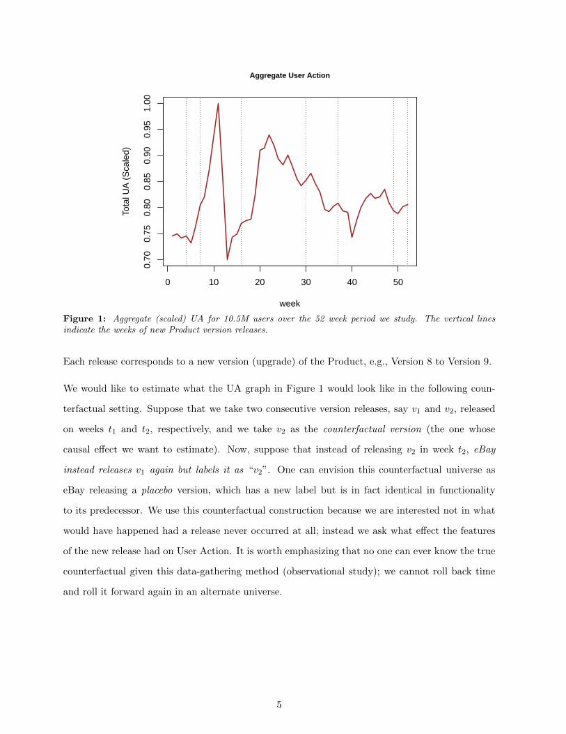
For the purposes of this paper, User Action is a normalized, non-negative, unit-less quantity
reported in user-action units (UAs). Higher aggregate values of UA imply higher (aggregate)
levels of satisfaction with the Product by the users in our study. A graph of weekly aggregate UA
over our 52-week study period is shown in Figure 1. The dashed vertical lines in Figure 1 indicate
weeks of Product releases: there were 7 unique releases (treatments) in our 52-week time window.
4
0 10 20 30 40 50
0.70
0.75
0.80
0.85
0.90
0.95
1.00
Aggregate User Action
week
Tota
l UA
(S
cale
d)
Figure 1: Aggregate (scaled) UA for 10.5M users over the 52 week period we study. The vertical linesindicate the weeks of new Product version releases.
Each release corresponds to a new version (upgrade) of the Product, e.g., Version 8 to Version 9.
We would like to estimate what the UA graph in Figure 1 would look like in the following coun-
terfactual setting. Suppose that we take two consecutive version releases, say v1 and v2, released
on weeks t1 and t2, respectively, and we take v2 as the counterfactual version (the one whose
causal effect we want to estimate). Now, suppose that instead of releasing v2 in week t2, eBay
instead releases v1 again but labels it as “v2”. One can envision this counterfactual universe as
eBay releasing a placebo version, which has a new label but is in fact identical in functionality
to its predecessor. We use this counterfactual construction because we are interested not in what
would have happened had a release never occurred at all; instead we ask what effect the features
of the new release had on User Action. It is worth emphasizing that no one can ever know the true
counterfactual given this data-gathering method (observational study); we cannot roll back time
and roll it forward again in an alternate universe.
5
2.2 Our Approach and Data
We approach the observational study problem from a longitudinal perspective and jointly model
the sequence of Product releases. Our dataset consists of the UA response for ≈ 10.5M eBay users
over an (undisclosed) 52 week period. The data is aggregated week by week, i.e., t = 1, . . . , T ,
where T = 52. For each user i = 1, . . . , n = 10,491,859, we have Product usage data (session logs)
broken out by version; i.e., for each week, we know which version of the Product a user had, and if
he (she) upgraded mid-week, we know the relative proportion of each version’s usage during that
week. A user was included in our study if he (she) was a registered eBay user as of the first day of
our study, and had at least one Product session logged in our 52-week window. Note: our response
UA is correlated with Product usage (number of sessions logged), but it is not the same as Product
usage. A frequent user (many logged Product sessions) can still have zero UAs logged.
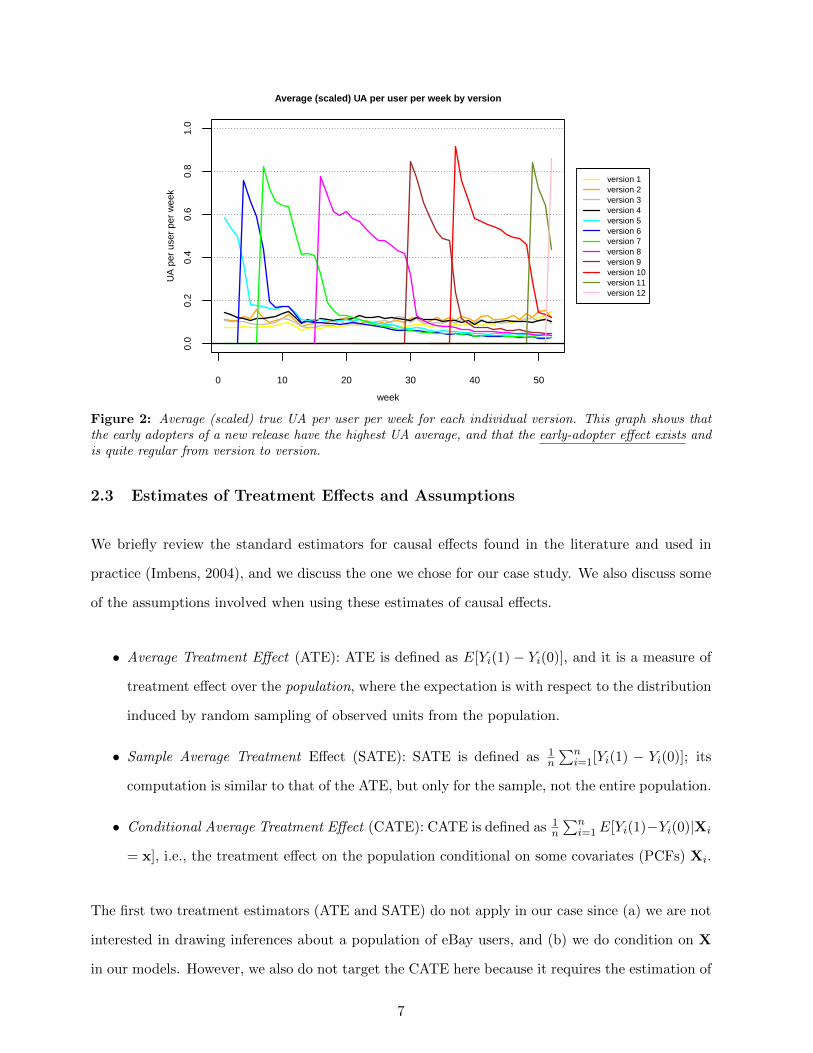
Figure 2: Average (scaled) true UA per user per week for each individual version. This graph shows thatthe early adopters of a new release have the highest UA average, and that the early-adopter effect exists andis quite regular from version to version.
2.3 Estimates of Treatment Effects and Assumptions
We briefly review the standard estimators for causal effects found in the literature and used in
practice (Imbens, 2004), and we discuss the one we chose for our case study. We also discuss some
of the assumptions involved when using these estimates of causal effects.
• Average Treatment Effect (ATE): ATE is defined as E[Yi(1)− Yi(0)], and it is a measure of
treatment effect over the population, where the expectation is with respect to the distribution
induced by random sampling of observed units from the population.
• Sample Average Treatment Effect (SATE): SATE is defined as 1n
∑ni=1[Yi(1) − Yi(0)]; its
computation is similar to that of the ATE, but only for the sample, not the entire population.
• Conditional Average Treatment Effect (CATE): CATE is defined as 1n
∑ni=1E[Yi(1)−Yi(0)|Xi
= x], i.e., the treatment effect on the population conditional on some covariates (PCFs) Xi.
The first two treatment estimators (ATE and SATE) do not apply in our case since (a) we are not
interested in drawing inferences about a population of eBay users, and (b) we do condition on X
in our models. However, we also do not target the CATE here because it requires the estimation of
7
two counterfactuals: Yi:Zi=0(1), the response of the C users if they had been treated, and Yi:Zi=1(0),
the response of the T users had they remained in the control group. Given the data resources in
our case study, we are able to reliably place the treated (upgraders) into the control group (non-
upgraders), but are not able to reliably predict who out of the non-upgraders would upgrade and
when they would upgrade.
Therefore, here we employ the Conditional Average Treatment (Effect) on the Treated (CATT)
as our measure of causal effect, initially similar to the above estimators but only dealing with the
treated group. CATT is defined as:
CATT =1
nT
∑i:Zi=1
E[Yi(1)− Yi(0)|Xi = x] . (1)
Three assumptions are relevant to the quality of CATT as a causal effect estimate.
• Ignorability assumption (Rosenbaum and Rubin, 1983): (Zi ⊥ Yi(0), Yi(1)|Xi = x). This
assumption states that if indeed all PCFs Xi have been controlled for, then treatment as-
signment Zi and response Yi are conditionally independent given the PCFs. If this is indeed
the case, it can be shown that the causal effect estimate will be unbiased (Rosenbaum and
Rubin, 1983). This assumption can essentially never be fully verified, because one can never
know if one has in fact controlled for all confounding factors.
• Overlap assumption for CATT (Heckman et al., 1997): Pr(Z = 1|X = xi) < 1. This
assumption states that when conditioning on some X = xi, one cannot have all subjects in
the treatment group: there must be some subjects in C, else one cannot estimate the effect
on the treated using the potential outcomes framework. This assumption can be verified to
some extent, and we do so in Appendix A.
• Stable Unit Treatment Value Assumption (SUTVA) (Imbens and Rubin, 2015). This assump-
tion states that the potential outcomes for any unit do not vary with the treatments assigned
to other units. In other words, whether a given subject is treated or not has no impact on
another subject’s response and vice-versa. We assume that SUTVA holds in our scenario be-
cause we have been told by eBay Product Managers that the particular eBay product under
consideration does not have a viral nature (e.g., an exponential adoption rate).
8
Under the ignorability assumption above, and for some flexible function (model) f , E[Yi(0)|Xi =
Simply put, the CCR is the ratio of the aggregate yCFi to the aggregate yi for the treated group.
All results below are reported in terms of CCR. Note that if∑
i:Zi=1 yCFi =∑
i:Zi=1 Yi, then
CCR=1, which means that the treatment had no causal effect on the response of the treated; CCR
values less than 1 suggest that the effect caused by the Product release was to increase UA (user
satisfaction) on average.
Extensive discussions with relevant eBay experts identified a strong source of information about
CCR external to our data: having launched a number of releases of the Product in the past without
dramatic apparent positive or negative effects on important indicators correlated with UA, company
experts were highly skeptical of CCR values far from 1. We use this (prior) information informally
as a kind of baseline in what follows.
2.4 Related Work
Our approach is fundamentally model-based, but other methods for causal inference in observa-
tional studies of course exist. As mentioned above, one leading approach to estimating causal
effects is via a comparison of potential outcomes. However, the problem is complicated by the
presence of unknown PCFs, and thus the problem boils down to controlling for such PCFs when
comparing responses in T and C.
One of the most widely used techniques relies on matching (Rubin, 1973) treated and control
subjects on the hypothesized PCFs (covariates), with the goal of achieving a balance in the covariate
distributions in the T and C groups (Rosenbaum and Rubin, 1985). Once a set of covariates is
identified, matching algorithms attempt to find the closest match to a treatment subject in the
9
control group, in a particular sense of closeness. Having identified the best control subject for each
treatment subject, the algorithm computes the average difference between the pairs of treatment
and control subjects. For a good review of matching techniques, see Stuart (2010).
One way to define the concept of closeness is through propensity score matching (Rosenbaum and
Rubin, 1983). The propensity score for a subject i is defined as the probability of receiving the
treatment given the observed covariates. There are two important properties of propensity scores.
First, at each value of the propensity score, the distribution of the covariates defining the score is
the same in the T and C groups, i.e., they act as balancing scores. Second, if treatment assignment
is ignorable given the covariates, it is also ignorable given the propensity score. Thus to compute
the causal effect, one can compare the mean responses of treated and control subjects having the
same propensity score. However, the above two properties only hold if one has found the true
propensity-score model: a poor estimate of the true propensity score will again lead to biased
causal effect estimates (Kang and Schafer, 2007). Besides matching on the propensity score, other
techniques involve using the propensity score in subclassification (Rosenbaum and Rubin, 1984),
weighting (Rosenbaum, 1987), regression (Heckman et al., 1997), and/or combinations of the above
(Rubin and Thomas, 2000). Bayesian analyses using propensity scores also exist (McCandless et al.,
2009).
Instrumental variables (IV) (Angrist et al., 1996) also have a long history, and are widely used in
econometrics as a way to approach unbiased causal estimates in the presence of PCFs. The key
idea behind IV is that if we can find an instrumental variable z with the property that it affects
the response y only through its effect on a PCF x and is uncorrelated with the error, then we can
still estimate the effect in an unbiased fashion. The issue is that such variables, whose only impact
on the response is indirectly through another covariate, are not easy to find in most situations.
The above approaches do not rely on any specific model of the data; they compare mean responses
between specially constructed samples of subjects from T and C. Model-based approaches (such
as ours in this paper) attempt to jointly model the treatment and the response in a flexible way so
that the unknown counterfactual potential outcomes can be estimated (predicted) by the model.
The models are typically linear regression models of the response, but can also be sophisticated
non-parametric models (e.g., decision trees) (Hill, 2011; Karabatsos and Walker, 2012). A recent
method utilizes a Bayesian time-series approach and a diffusion-regression state-space model to
10
Version n Treated n Control Unadjusted CCR PCF-Adjusted CCR
5 3638K 561K 1.35 1.14
7 3838K 704K 1.32 1.10
Table 1: Previous (simple) attempts at answering the causal effect question led to unrealistic causal effectestimates. Unadjusted refers to a simple comparison of means (null model); PCF-adjusted refers to regressionmodels with a variety of PCFs as covariates, and is based on the CATE estimator.
estimate the causal effect of an advertising campaign (Brodersen et al., 2015); this approach is
closest in spirit to our methodology, but it analyzes the effect of only a single intervention.
2.5 Previous eBay Causal Estimates
We now describe a previous approach at eBay to the above causal inference problem; the method
focused on analyzing the causal effect of one release at a time. A pool of users was selected based
on activity logs in a ± 2 week window around the release in question (the counterfactual release).
The pool of users was then divided into T and C groups based on their version usage during the
pre-release and post-release window. The UA for both groups was computed in a 2 week window
before the release, and in a 2 week window that started 3 days (burn-in) after the day of Product
release. The results are given in Table 1. A simple (unadjusted) estimate using the means of the
treatment and control groups shows CCR values in excess of 1.30 (enormous in relative terms),
naively implying a huge effect of the release on customer satisfaction. The PCF-adjusted CCR
(1.10 to 1.14) was computed using the CATE version of the CCR estimator described above, using
a regression model that included hypothesized PCFs as covariates. No one in the organization
believed the unadjusted estimates, and although the PCF-adjusted numbers were more reasonable,
no one believed them either because they were still large in relative terms. Therefore, a new
approach was necessary. (Note that the results were similar for two releases, suggesting that each
release had a significant impact on UA, further eroding the credibility of this approach.)
3 Model and Design Matrices
We fit our data using variations of a Bayesian hierarchical (mixed effects) model with a Gaussian
error distribution (see Section 5.2 for sensitivity analyses of this choice of model class). Many of
the models we examined include auto-regressive (AR) terms of different orders p. In such cases, we
11
use the standard conditional-likelihood approach (Reinsel, 2013) to building the likelihood function
with AR terms; this is justified in our case because (a) our outcome variable, with a reasonable
number of AR lags, is essentially stationary, and (b) the modeling has the property that the X
matrix, when the AR model is estimated via regression, is invertible. This permits us to regard
the fi matrix for each user i as a matrix of fixed known constants in the models below.
The dimensions of all the quantities listed below are as follows, where p denotes the AR order.
• yi: a (T − p) by 1 vector of user i’s response (UA);
• βi: a d by 1 vector; in random effects models, d is the length of the random effects coefficients
vector, and includes the AR coefficients;
• fi: a (T − p) by d matrix of constants and lagged yi values (see Section 3.1);
• Wi: a (T − p) by (T − p) matrix of fixed known constants (typically week indicators); and
• γ : a (T − p) by 1 vector of coefficients of the fixed effects.
Our primary working model is a mixed-effects hierarchical model with Gaussian error. For user
i = 1, . . . , n =10,491,859, the model is as follows:
yi = fi βi + Wi γ + εi
(βi |µ,Σ) ∼ N(µ,Σ)
(εi | ν) ∼ N(0, νIT−p)
µ ∼ N(0, κµId)
γ ∼ N(0, κγIT−p)
ν ∼ Inv-Gamma( ε
2,ε
2
)Σ ∼ Inv-Wishartd+1(I) (4)
This model assumes that each Product version affects all users differently, i.e., the model treats all
users in a heterogeneous fashion, and allows room for homogeneous fixed-effects common to all users
in the Wi matrix. We assume the error distribution to be Gaussian. This is quite possibly incorrect
12
for individual users, but can still lead to a model that performs well in the aggregate; section 5.2
shows that our results are insensitive to an alternative non-parametric error specification.
We employ diffuse (yet proper) priors for µ,γ, and ν, namely κµ = κγ = 106, and ε = 0.001.
For the prior on the unknown covariance matrix Σ, we choose a diffuse proper prior distribution
(Gelman et al., 2014) which has the nice feature that each single correlation in the Σ matrix has
marginally a uniform prior distribution. We fit the above mixed-effects model using MCMC, and all
full conditional distributions are available in closed form (see Appendix B.1). Sensitivity analyses
not presented here demonstrated that reasonable variations in the hyper-parameters of the diffuse
priors had negligible effects on the results, which is to be expected with n in excess of 10 million.
3.1 fi Matrix
For each user i, the design matrix fi contains three sets of covariates: (a) the version (treatment)
indicators, (b) the PCFs that encode waiting time to adopt the latest version, and (c) other user
covariates. We detail each of these below.
3.1.1 Version (Treatment) Indicators
The R = 12 version indicator columns of fi denote which specific version (treatment) user i had
installed during each of the T = 52 weeks. In detail, fversioni = [x′i,1,x
′i,2, . . . ,x
′i,R]
′, where r =
1, . . . , R = 12 is the number of unique Product versions in the study. Each indicator column xi,r
encodes the weeks user i had version r. In the vast majority of cases, xi,r only contains 0/1 values;
however, we allow for fractional entries in cases where a user upgraded to a new version midweek.
We compute such fractional usage using session data for a given week.
3.1.2 Waiting Time PCFs
To control for the early-adopter effect mentioned above, we construct 14 binary indicator variables
called n-weeks-past-release indicators. For a given user i in a given week t, we calculate how long
ago the current latest version was released, relative to the given week t. For instance, suppose
that the current latest version was shipped in week t1, and the given week is t; then n-weeks-past-
release(t) = (t−t1). We then set the (t−t1)-th indicator variable to 1. There are 14 such indicators
Table 2: Example of a user’s n-weeks-past-release indicator columns fwaiting timei . The “.” entries represent
0. The horizontal lines indicate weeks of new version releases. This user waited 3 weeks to upgrade to theversion released in week 0 (t = 0), and waited 1 week to upgrade to the version released in week 7 (t = 7).
because that is the maximum number of weeks between consecutive releases. Table 2 presents an
example of this calculation for a single user.
3.1.3 Other Covariates
Looking at all of our 10.5M users, we have approximately 2.83M users whose first recorded Product
usage was during our 52 week window. (This is not to say these users had never used the Product
before, but we did not find a record of them using the Product in the 12 months prior to the start
of our study). Thus we include a binary indicator covariate called virgin user to denote those
users who appeared to use the Product for the first time ever in our study window. We also add
a covariate that captures a user’s long term behavior, namely the six-month rolling average of UA
over all of eBay’s products, not just using the Product in the study. Finally, in order to control for
a user’s behavior during the one week he or she upgrades, we include a binary indicator covariate
(upgrade-week) for the particular week in which an upgrade occurs.
3.2 Wi Matrix
Our initial exploratory (flat) model assumed that each Product version affects all users equally,
i.e., the model treats all users in a homogeneous fashion by having a single β parameter instead
14
of the βi random effects in model (4). We initially captured this idea with the following ordinary
least squares (OLS) Gaussian model: for user i = 1, . . . , n =10,491,859,
yi = fiβ + Wiγ + εi
(εi | ν) ∼ N(0, νIT−p)
(β,γ, ν) ∝ 1 . (6)
We immediately found it necessary to account for time in some manner. Models that did not
account for time at all, and models that involved a simple linear time variable (t), did poorly in
fitting the aggregate response. We discovered that our best models were those that included an
effect for each individual specific week of our 52-week period. Therefore, we included (T−p) (where
p is the AR order) indicator columns as fixed effects in the matrix Wi in model (6); each Wi is
effectively the identity matrix of dimension (T − p). These indicator variables can be regarded
as proxying for changes over time that are exogenous to our study, both internal and external to
eBay.
3.3 Counterfactual fi Matrix
Throughout our work we estimated the counterfactual response YCF , given a certain Product
version, which we call the counterfactual version (CV). As noted in Section 2.1, we estimate the
response (UA) if that particular version had not been released, but a placebo version had been
released in its place.
When estimating the counterfactual response, we need a counterfactual counterpart to the version
indicator columns described above, namely fCF versioni . We construct fCF version
i by simply moving
the user from the CV to his or her previous version (note that this is user-dependent). In the
fversioni matrix, this amounts to adding the CV indicator column to the column corresponding to
the user’s prior version, and then zeroing out the CV column. The counterfactual for a virgin user
is constructed by moving the user to the most recent previous version.
There is a slight twist to computing counterfactual estimates in models that include auto-regressive
AR(p) terms, as many of our models do. Suppose that we include an AR(1) term in as a random
effect. In this case, we have to make an adjustment in the counterfactual computation during the
15
time period in which the CV was active: the true lagged y values are replaced by their (sequentially)
estimated lagged y values, but only during the period of time during which the CV was employed
by the given user.
3.4 Counterfactual Computation
The estimate of the counterfactual YCF response in our hierarchical mixed-effects model is com-
puted as follows. Given that we have fit the model and run M samples after burn-in, we have the
following sets of samples from the posterior distributions above:
• M samples each of µ, Σ, γ, and ν; and
• βi : Since we have n = 10.5 million users in our dataset, and finite memory and disk space,
we do not store M samples of each user’s d dimensional vector βi. Instead, we simply store
the mean βi for each user i, where the mean is taken over the M posterior samples.
Given the above, we calculate the counterfactual estimates as follows. If we are just interested in
point estimates, we simply use the point estimates βi from the posterior for each user i:
yCFi = fCFi βi + Wiγ . (7)
To create uncertainty bands around our estimate, we simulate the following. For each user i, we
draw β∗i from the its full conditional given the true fi matrix and the posterior means of the other
parameters, and then draw yCFi using the counterfactual fCFi matrix:
β∗i ∼ p(βi|yi, fi, µ, Σ, ν, γ)
yCFi ∼ N(fCFi β∗i + Wiγ, ν) . (8)
We then sum up each user’s CF estimate to obtain the aggregate estimate YCF =∑n
i=1 yCFi . Note
that our CATT estimates only consider the counterfactual response during the weeks of a release’s
lifetime, i.e., when it was the latest release on the market. In the case of Version 9, this period was
from week 30 up to and including week 36, and we make no claims about the counterfactual story
thereafter, at which point Version 10 comes on the market. The reason for this is as follows. In our
16
counterfactual constructed universe, during the 7 weeks in which Version 9 was the latest version,
users were shifted onto the release they had immediately prior to Version 9 (this varied among
users, but the majority were on Version 8). When Version 10 was released, users who upgraded to
Version 10 in the true universe were upgraded in the CF universe as well, but users who remained
on Version 9 in the true universe were retained on Version 8. In the window where Version 9
was the latest release on the market (the only game in town, so to speak), this is the only choice
available to us. However, when Version 10 replaces Version 9 as the latest release, we cannot be
sure those same users who stuck with Version 9 until the end would have also stuck with Version
8 until the end.
4 Estimates of Treatment Effects
In order to motivate our methodology and results, we first demonstrate what happens when one
models an individual version release in isolation and also ignores the early-adopter effect. Next
we show that more reasonable estimates are achieved when one takes the early-adopter effect into
account, and in order to do so, one must model the entire sequence of version releases. In the
following causal effect estimates, we take Version 9 as our counterfactual version released in week
30 (and replaced in week 37) in all models initially; once we have settled on the best model, we
apply the same CF estimation technique to Version 10 (released in week 37).
4.1 Modeling a Single Version in Isolation
As a first step, we ignore the early-adopter effect completely and estimate the causal effect of
Version 9 in isolation. Our first reduced model (model MaR) includes weeks 24 through 36 only, only
Versions 1 through 9, and does not include the 14 n-weeks-past-release indicators. The results for
this are given in Figure 3. The estimate of the mean CCR for Version 9 from model MaR is 0.906,
which implies that without Version 9, the UA of the treated would have been around 10% lower in
aggregate over weeks 30–36. This is not credible given the informal prior information from eBay
Product Managers described in Section 2.3; moreover, the right-hand panel in Figure 3 shows that
this model fits the responses of the users in the treatment group poorly in the run-up to the release
of Version 9.
17
0 10 20 30 40 50
0.70
0.75
0.80
0.85
0.90
0.95
1.00
All users
week
UA
YY_hatY_hat_cf
0 10 20 30 40 50
0.6
0.7
0.8
0.9
1.0
5M treated
week
UA
YY_hatY_hat_cf
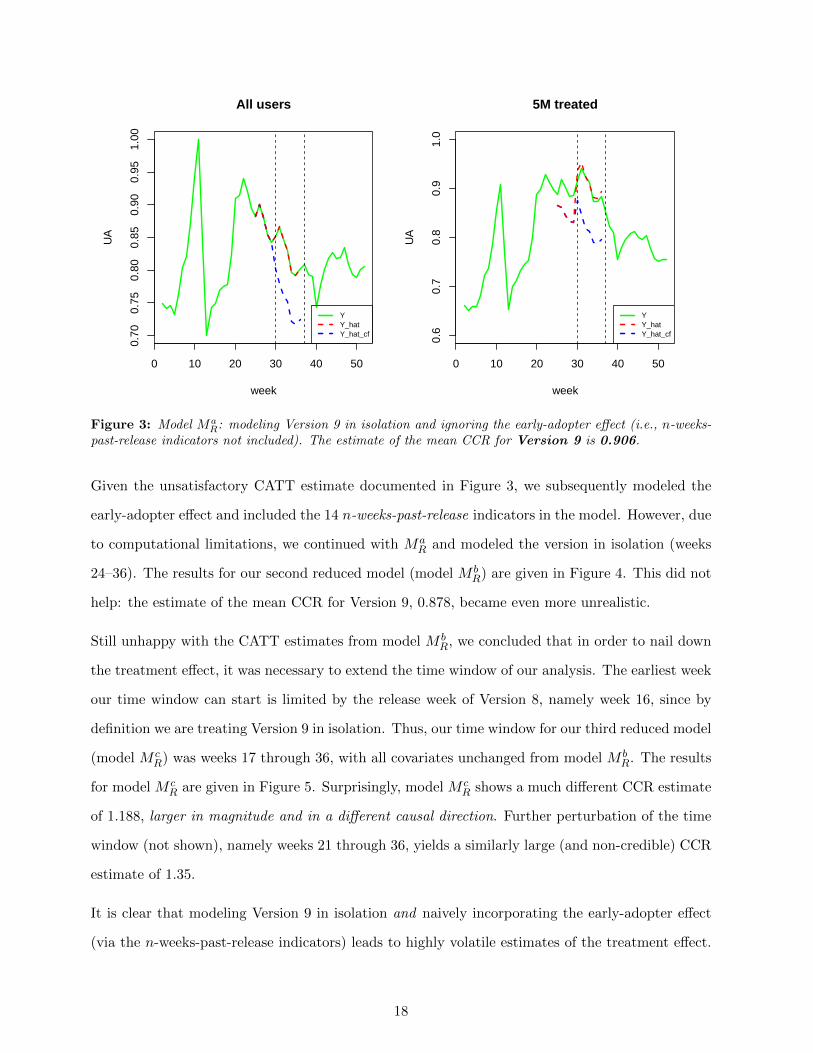
Figure 3: Model MaR: modeling Version 9 in isolation and ignoring the early-adopter effect (i.e., n-weeks-
past-release indicators not included). The estimate of the mean CCR for Version 9 is 0.906.
Given the unsatisfactory CATT estimate documented in Figure 3, we subsequently modeled the
early-adopter effect and included the 14 n-weeks-past-release indicators in the model. However, due
to computational limitations, we continued with MaR and modeled the version in isolation (weeks
24–36). The results for our second reduced model (model M bR) are given in Figure 4. This did not
help: the estimate of the mean CCR for Version 9, 0.878, became even more unrealistic.
Still unhappy with the CATT estimates from model M bR, we concluded that in order to nail down
the treatment effect, it was necessary to extend the time window of our analysis. The earliest week
our time window can start is limited by the release week of Version 8, namely week 16, since by
definition we are treating Version 9 in isolation. Thus, our time window for our third reduced model
(model M cR) was weeks 17 through 36, with all covariates unchanged from model M b
R. The results
for model M cR are given in Figure 5. Surprisingly, model M c
R shows a much different CCR estimate
of 1.188, larger in magnitude and in a different causal direction. Further perturbation of the time
window (not shown), namely weeks 21 through 36, yields a similarly large (and non-credible) CCR
estimate of 1.35.
It is clear that modeling Version 9 in isolation and naively incorporating the early-adopter effect
(via the n-weeks-past-release indicators) leads to highly volatile estimates of the treatment effect.
18
0 10 20 30 40 50
0.70
0.75
0.80
0.85
0.90
0.95
1.00
All users
week
UA
YY_hatY_hat_cf
0 10 20 30 40 50
0.6
0.7
0.8
0.9
1.0
5M treated
week
UA
YY_hatY_hat_cf
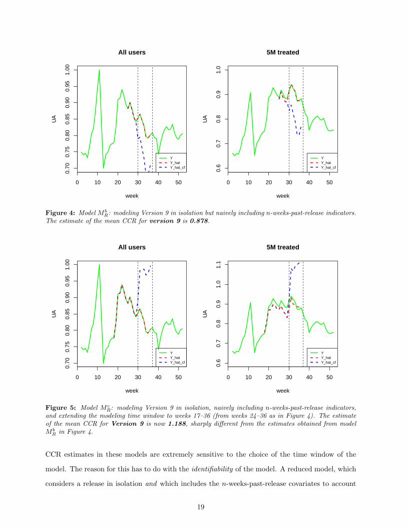
Figure 4: Model M bR: modeling Version 9 in isolation but naively including n-weeks-past-release indicators.
The estimate of the mean CCR for version 9 is 0.878.
0 10 20 30 40 50
0.70
0.75
0.80
0.85
0.90
0.95
1.00
All users
week
UA
YY_hatY_hat_cf
0 10 20 30 40 50
0.6
0.7
0.8
0.9
1.0
1.1
5M treated
week
UA
YY_hatY_hat_cf
Figure 5: Model M cR: modeling Version 9 in isolation, naively including n-weeks-past-release indicators,
and extending the modeling time window to weeks 17–36 (from weeks 24–36 as in Figure 4). The estimateof the mean CCR for Version 9 is now 1.188, sharply different from the estimates obtained from modelM b
R in Figure 4.
CCR estimates in these models are extremely sensitive to the choice of the time window of the
model. The reason for this has to do with the identifiability of the model. A reduced model, which
considers a release in isolation and which includes the n-weeks-past-release covariates to account
19
for the early-adopter effect, runs the risk of being non-identifiable because by construction the
treatment indicator column approaches a linear combination of the n-weeks-past-release indicator
columns: in model M bR (weeks 24–36), the correlation between the Version 9 indicator column and
the sum of the first 7 “n-weeks-past-release” columns was 0.984. The correlation was computed
over all 10.5M users for the 12-week time window (13 weeks minus 1 for AR(1)); the constructed
(126M × 1)-dimensional vectors differed in fewer than 0.7% of the locations. Clearly models with
such collinear covariates are on the edge of identifiability, leading to wildly varying estimates of
parameters and consequently of treatment effects. Furthermore, this makes it is almost impossible
to isolate the early-adopter effect from the version treatment effect. Nevertheless, the early-adopter
effect is real (recall Figure 2) and must be accounted for.
4.2 Modeling All Versions Jointly
The straightforward approach to deal with the identifiability problem is to model all treatments
jointly in a full model, and include covariates (PCFs) that explicitly encode each user’s waiting time
to adopt the treatment. Pooled data from other treatments reduces the collinearity in the design
matrices because different users play the role of early adopters in each release. This may be seen
by computing the correlation between the same covariate vectors in the full model (as we did in
reduced model); the new value of only 0.216 means that there is little overlap between sets of early
adopters from one version to the next. This allows for robust estimates of the early-adopter effect,
i.e., of the values of the n-weeks-past-release coefficients, which in turn produces robust estimates
of the treatment indicator coefficients and a realistic CATT estimate. These results are given in
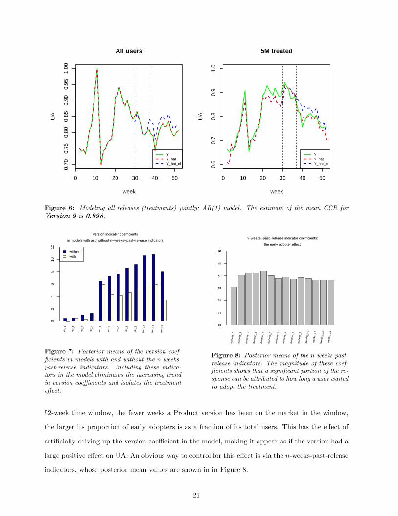
Figure 6. The estimated mean CCR value for Version 9 is 0.998, a negligible causal effect.
The early-adopter effect can also clearly be seen in Figures 7 and 8. Figure 7 shows the posterior
means of the components of µ that correspond to the 12 versions (i.e., the version coefficients)
resulting from two models: first, a model that ignores the early-adopter effect and excludes the
n-weeks-past-release indicators, and second, a model that does include these indicators. Note that
in the first model, the version coefficients show an increasing trend, because the early-adopter effect
is confounded with the treatment effect. (Version 12’s coefficient does not follow the trend because
Version 12 appears in only the last week in our study (week 52); in this case, the upgrade-week
indicator accounts for the first-week-adopter effect). The confounding occurs because, given a fixed
20
0 10 20 30 40 50
0.70
0.75
0.80
0.85
0.90
0.95
1.00
All users
week
UA
YY_hatY_hat_cf
0 10 20 30 40 50
0.6
0.7
0.8
0.9
1.0
5M treated
week
UA
YY_hatY_hat_cf
Figure 6: Modeling all releases (treatments) jointly; AR(1) model. The estimate of the mean CCR forVersion 9 is 0.998.
withoutwith
Version indicator coefficients
in models with and without n−weeks−past−release indicators
02
46
810
12
ver_
1
ver_
2
ver_
3
ver_
4
ver_
5
ver_
6
ver_
7
ver_
8
ver_
9
ver_
10
ver_
11
ver_
12
Figure 7: Posterior means of the version coef-ficients in models with and without the n-weeks-past-release indicators. Including these indica-tors in the model eliminates the increasing trendin version coefficients and isolates the treatmenteffect.
n−weeks−past−release indicator coefficients:
the early adopter effect
01
23
45
6
nwee
ks_0
nwee
ks_1
nwee
ks_2
nwee
ks_3
nwee
ks_4
nwee
ks_5
nwee
ks_6
nwee
ks_7
nwee
ks_8
nwee
ks_9
nwee
ks_1
0
nwee
ks_1
1
nwee
ks_1
2
nwee
ks_1
3
Figure 8: Posterior means of the n-weeks-past-release indicators. The magnitude of these coef-ficients shows that a significant portion of the re-sponse can be attributed to how long a user waitedto adopt the treatment.
52-week time window, the fewer weeks a Product version has been on the market in the window,
the larger its proportion of early adopters is as a fraction of its total users. This has the effect of
artificially driving up the version coefficient in the model, making it appear as if the version had a
large positive effect on UA. An obvious way to control for this effect is via the n-weeks-past-release
indicators, whose posterior mean values are shown in in Figure 8.
21
5 Model Selection and Validation
Our goals in model selection and validation are twofold: (a) choose the single best model so that
we can accurately estimate the CCR for other versions, and (b) make sure that our results are
relatively robust to over-fitting. Therefore, we study the sensitivity of our results to different AR
orders, as well as investigate two additional model classes: the simpler flat model with a Gaussian
error distribution given in equation (6), and a more complex model with a non-parametric error
distribution. Finally, we perform 5-fold cross-validation to verify that our results are not sensitive
to some random subset of our users.
Our primary selection criterion for a best model is the the fit-of-the-treated, namely the in-sample
root-mean-squared-error (RMSE) on the treatment group. The reasons for this are two-fold. First,
we are interested in computing CATT, namely the effect on the treatment group. Second, we
are (currently) not interested in predicting aggregate UA into the future, nor are we interested in
predicting how another totally different set of users would behave. We are focused on accurately
modeling our in-sample 10.5M users (and the approximately 5M treated ones in particular) so
that we can ascertain what their behavior would have been like in the counterfactual world. The
secondary selection criteria is scalability (computational feasibility). Given that we are doing
Bayesian inference over 10.5M users in an approximately 80-dimensional space, the ability to fit
the model in a reasonable amount of time is important. If a model takes an inordinate amount of
time to fit, its performance advantage over competing models should be commensurate with this
increased time and effort.
5.1 AR Order Sensitivity
Table 3 gives the results for three identical hierarchical models in which we perturbed the AR
order: p = {0, 1, 4}. It is evident that the overall estimates of the causal effect — as measured by
the posterior mean of CCR for Version 9 — are relatively insensitive to the AR order. However,
the AR(4) model performs better than the AR(0) and AR(1) models (with minimal computational
overhead), so we proceed with the AR(4) model in all subsequent analyses.
22
ErrorModel Class Distribution AR order RMSE Before RMSE After Mean CCR
Hierarchical Normal 0 57.88 68.61 0.984
Hierarchical Normal 1 56.55 66.96 0.998
Hierarchical Normal 4 53.64 63.35 1.004
Table 3: RMSE [ 1nT
(YT −YT )2]1/2 for the treated users over 7 weeks before and 7 weeks after the releaseof Version 9. The (posterior) mean CCR results are relatively insensitive to the AR order of the model, butmore heterogeneity (i.e., a larger AR order) leads to a better fit of the treated.
5.2 Sensitivity to Model Class
Having selected an AR(4) hierarchical model as our best candidate so far, we now study results
from the simpler flat model (6) with a Gaussian error distribution and from a more complex model
with a non-parametric error distribution.
• First, we do not fit the flat OLS model because we consider it a sensible reflection of reality;
it is not credible that all 10.5M users can be treated in a homogeneous fashion. However, it
is a limiting case of our hierarchical model in which Σ → 0, and thus is a good candidate
for analysis. In the last line of model (6) we assume an (improper) diffuse prior for all the
• Second, we fit the following Bayesian non-parametric (BNP) error model: for user i =
1, . . . , n = 10,491,859,
yi = fiβi + Wiγ + εi
(εi | θi, ν) ∼ N(θi 1T−p, ν IT−p)
(θi | P) ∼ P
P ∼ DP(α,P0) α = 3 (fixed)
P0 = N(0, τ0) τ0 = 100 (fixed)
βi ∼ N(µ,Σ)
(ν,µ,Σ,γ) : as in equation (4) . (9)
Model (9) is an expansion of our main hierarchical model (4), in that it allows the error
distribution to have a (more realistic) non-parametric form, namely a Dirichlet process (DP)
23
mixture of Gaussians. The idea is that the non-parametric DP (location) mixture form of the
error distribution will do a better job fitting the small percentage of high UA users. We fit
model (9) using the marginal Gibbs sampler (Gelman et al., 2014). (Varying α and τ0 across
reasonable ranges had little effect on the results.)
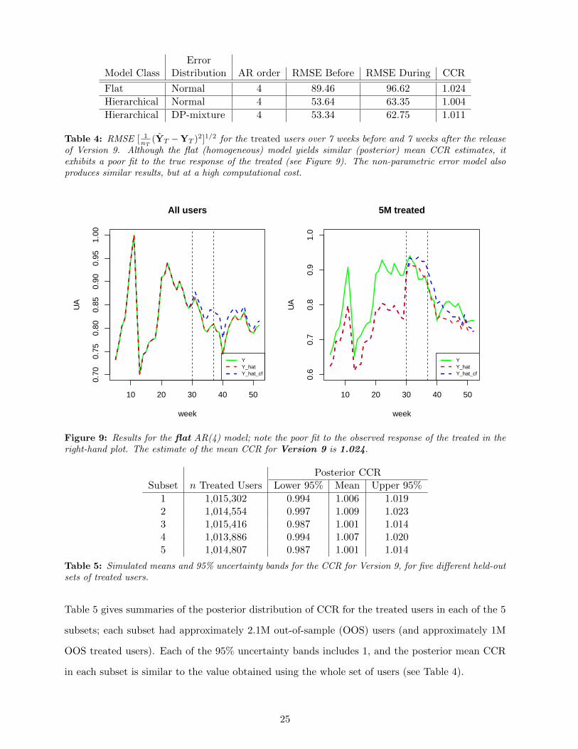
The results for different model classes are shows in Table 4; we have included the Normal
hierarchical model as well for comparison. Evidently, given the same covariates, all three
models produce similar CCR estimates. However, note that the flat model does an extremely
poor job of fitting the treated users. Figure 9 graphically illustrates this lack of in-sample fit
to the treated. Without the benefit of similar CCR estimates from the hierarchical model,
its CCR estimate of 1.024 would be hard to believe given such a poor fit to the treated. This
illustrates the importance of taking user heterogeneity into account, especially when one is
trying to estimate the causal effect on the treated.
At the other end of the model complexity spectrum, Table 4 shows that the BNP model
fit slightly better but yielded a CCR estimate that is similar to that from the hierarchical
Gaussian model: the posterior mean CCR moved from 1.004 to 1.011. However, this came at
a great computational cost: it took approximately 3 times the amount of clock time (with the
same hardware) to fit the DP mixture model as it did the Gaussian hierarchical model with
the same exact covariates. Since the model with the non-parametric error distribution shows
only minor differences in the CCR estimates, we argue that although its error distribution may
be more realistic at the individual user level, it does not practically matter when considering
the aggregate (and the mean) response. As we mentioned previously, the error distribution
for any single user is not Gaussian, but the lack of sensitivity to the exact form of error
distribution at the aggregate level allows us to use the simpler hierarchical Gaussian model
(4) with a reasonable degree of confidence.
5.3 5-fold Cross Validation
Given that the hierarchical Gaussian AR(4) model is our chosen model, we performed 5-fold cross-
validation to check its out-of-sample (OOS) predictions. We fit 5 different variants of it using
only 80% of the users each time, and examined the fit and computed the CCR estimates on the
remaining 20% of the users.
24
ErrorModel Class Distribution AR order RMSE Before RMSE During CCR
Flat Normal 4 89.46 96.62 1.024
Hierarchical Normal 4 53.64 63.35 1.004
Hierarchical DP-mixture 4 53.34 62.75 1.011
Table 4: RMSE [ 1nT
(YT −YT )2]1/2 for the treated users over 7 weeks before and 7 weeks after the releaseof Version 9. Although the flat (homogeneous) model yields similar (posterior) mean CCR estimates, itexhibits a poor fit to the true response of the treated (see Figure 9). The non-parametric error model alsoproduces similar results, but at a high computational cost.
10 20 30 40 50
0.70
0.75
0.80
0.85
0.90
0.95
1.00
All users
week
UA
YY_hatY_hat_cf
10 20 30 40 50
0.6
0.7
0.8
0.9
1.0
5M treated
week
UA
YY_hatY_hat_cf
Figure 9: Results for the flat AR(4) model; note the poor fit to the observed response of the treated in theright-hand plot. The estimate of the mean CCR for Version 9 is 1.024.
Posterior CCRSubset n Treated Users Lower 95% Mean Upper 95%
Table 5: Simulated means and 95% uncertainty bands for the CCR for Version 9, for five different held-outsets of treated users.
Table 5 gives summaries of the posterior distribution of CCR for the treated users in each of the 5
subsets; each subset had approximately 2.1M out-of-sample (OOS) users (and approximately 1M
OOS treated users). Each of the 95% uncertainty bands includes 1, and the posterior mean CCR
in each subset is similar to the value obtained using the whole set of users (see Table 4).
25
10 20 30 40 50
0.0
0.2
0.4
0.6
0.8
1.0
Y_hat OOS posterior uncertainty bands (number of users = 1,000).
week
UA
true yy_hat oos meany_hat oos 95% interval
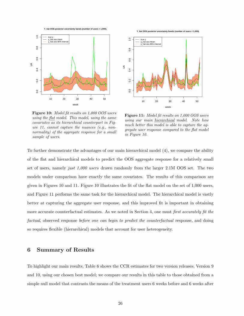
Figure 10: Model fit results on 1,000 OOS usersusing the flat model. This model, using the samecovariates as its hierarchical counterpart in Fig-ure 11, cannot capture the nuances (e.g., non-normality) of the aggregate response for a smallsample of users.
10 20 30 40 50
0.0
0.2
0.4
0.6
0.8
1.0
Y_hat OOS posterior uncertainty bands (number of users = 1,000).
week
UA
true yy_hat oos meany_hat oos 95% interval
Figure 11: Model fit results on 1,000 OOS usersusing our main hierarchical model. Note howmuch better this model is able to capture the ag-gregate user response compared to the flat modelin Figure 10.
To further demonstrate the advantages of our main hierarchical model (4), we compare the ability
of the flat and hierarchical models to predict the OOS aggregate response for a relatively small
set of users, namely just 1,000 users drawn randomly from the larger 2.1M OOS set. The two
models under comparison have exactly the same covariates. The results of this comparison are
given in Figures 10 and 11. Figure 10 illustrates the fit of the flat model on the set of 1,000 users,
and Figure 11 performs the same task for the hierarchical model. The hierarchical model is vastly
better at capturing the aggregate user response, and this improved fit is important in obtaining
more accurate counterfactual estimates. As we noted in Section 4, one must first accurately fit the
factual, observed response before one can begin to predict the counterfactual response, and doing
so requires flexible (hierarchical) models that account for user heterogeneity.
6 Summary of Results
To highlight our main results, Table 6 shows the CCR estimates for two version releases, Version 9
and 10, using our chosen best model; we compare our results in this table to those obtained from a
simple null model that contrasts the means of the treatment users 6 weeks before and 6 weeks after
26
Posterior CCRVersion Model Lower 95% Mean Upper 95%
9 Null 0.815 0.824 0.833
9Hierarchical AR(4),
Normal Errors0.998 1.004 1.010
10 Null 0.709 0.720 0.731
10Hierarchical AR(4),
Normal Errors1.022 1.028 1.035
Table 6: Summary of causal effect estimates for Versions 9 and 10. The null model is a simple naivecomparison of means for the treated group in a 6-week time window before and after the respective versionrelease.
each release (results were similar with ± time windows other than 6). The null CCR estimates
are wildly different from 1 on the low side, reflecting the magnitude of the early-adopter effect;
the hierarchical estimates are close enough to 1 to allay any eBay fears of highly defective Product
releases.
In conclusion, we have shown that careful consideration of long-term patterns of user behavior
combined with flexible models yields causal estimates that are reasonable and stable. If the response
to a treatment exhibits the characteristics of an early-adopter effect, then it is essentially impossible
to isolate the causal effect of the treatment by analyzing a single treatment event in isolation.
Attempting to do so (without including the appropriate PCFs) will yield treatment-effect estimates
that are either unrealistic or unstable, because of model identifiablity issues. However, if the early-
adopter effect exhibits a relatively consistent pattern from one treatment event to the next, we
can estimate its contribution to the overall response by jointly modeling many similar treatment
events simultaneously.
Obtaining convincing CATT estimates requires doing a good job on the (in-sample) fit of the
treated, which in turn requires flexible models that account for user heterogeneity. Hierarchical
mixed-effects Bayesian models similar to the one presented here offer a good solution, for two
reasons. First, models in which each user has her/his own random effect naturally account for
heterogeneity. Second, the hierarchical nature of the model makes it possible to borrow strength
across multiple treatment events, permitting isolation of the early-adopter effect from the treatment
Table 7: Quantiles of π. Fewer than 0.01% (0.0069% to be exact) of the treated violate the π < 1 condition.
Appendices
A CATT (Weak) Overlap Assumption
For CATT estimates, it is sufficient that we verify π ≡ Pr(Z = 1|X) < 1 (Heckman et al., 1997).
To do so we build a simple (linear) logistic regression model of the treated and control groups
using our best covariates. We collapse all of the n-weeks-past-release binary indicators into a single
summed integer value in the range of [0, 13]. The estimated density plot of the resulting fitted
probabilities π from the logistic regression model is shown in figure 12. We can see that for the
most part, π < 1 is indeed true, except for a very few cases. How few? If we look at the quantiles
of the fitted probability scores, we see the distribution in table 7. We see that the assumption
holds for nearly all treated users; it fails in only 0.0069% of cases.
0.0 0.2 0.4 0.6 0.8 1.0
0.0
0.5
1.0
1.5
2.0
2.5
3.0
Density Estimate of Pr(W=1|X)
p(Treated)
Figure 12: Density estimate of the fitted propensity score π from a linear model, i.e. the probability ofbeing in the treatment group conditional on the covariates.