arX

iv:h

ep-t

h/06

0217

8v2

31

Mar

200

6

CERN-PH-TH/2006-033HUTP-06/A0005

Causality, Analyticity and an

IR Obstruction to UV Completion

Allan Adamsa, Nima Arkani-Hameda, Sergei Dubovskya,b,c,

Alberto Nicolisa, Riccardo Rattazzib1

a Jefferson Physical Laboratory,

Harvard University, Cambridge, MA 02138, USA

b CERN Theory Division, CH-1211 Geneva 23, Switzerland

c Institute for Nuclear Research of the Russian Academy of Sciences,

60th October Anniversary Prospect, 7a, 117312 Moscow, Russia

Abstract

We argue that certain apparently consistent low-energy effective field theories described by local, Lorentz-

invariant Lagrangians, secretly exhibit macroscopic non-locality and cannot be embedded in any UV

theory whose S-matrix satisfies canonical analyticity constraints. The obstruction involves the signs

of a set of leading irrelevant operators, which must be strictly positive to ensure UV analyticity. An

IR manifestation of this restriction is that the “wrong” signs lead to superluminal fluctuations around

non-trivial backgrounds, making it impossible to define local, causal evolution, and implying a surprising

IR breakdown of the effective theory. Such effective theories can not arise in quantum field theories or

weakly coupled string theories, whose S-matrices satisfy the usual analyticity properties. This conclusion

applies to the DGP brane-world model modifying gravity in the IR, giving a simple explanation for the

difficulty of embedding this model into controlled stringy backgrounds, and to models of electroweak

symmetry breaking that predict negative anomalous quartic couplings for the W and Z. Conversely, any

experimental support for the DGP model, or measured negative signs for anomalous quartic gauge boson

couplings at future accelerators, would constitute direct evidence for the existence of superluminality and

macroscopic non-locality unlike anything previously seen in physics, and almost incidentally falsify both

local quantum field theory and perturbative string theory.

1On leave from INFN, Pisa, Italy.

1 Introduction

Can every low-energy effective theory be UV completed into a full theory? To a string theoristin 1985, the answer to this question would have been a resounding “no.” The hope was that theconsistency conditions on a full theory of quantum gravity would be so strong as to more or lessuniquely single out the standard model coupled to GR as the unique low-energy effective theory,and that the infinite number of other possible effective theories simply couldn’t be extended to afull theory. In support of this view, the early study of perturbative heterotic strings yielded manyconstraints on the properties of the low-energy theory invisible to the effective field theorist. Forinstance, the rank of the gauge group was restricted to be smaller than 22.

With the discovery of D-branes and the duality revolution, these constraints appear to haveevaporated, leaving us with a continuous infinity of consistent supersymmetric theories coupledto gravity and very likely a huge discretum of non-supersymmetric vacua [1]. If the low-energytheory describing our universe is not unique but merely one point in a vast landscape of vacua ofthe underlying theory, then the properties of our vacuum—such as the values of the dimensionlesscouplings of the standard model—are unlikely to be tied to the structure of the fundamental theoryin any direct way, reducing the detailed study of its particle-physical properties to a problem ofonly parochial interest. This situation is not without its consolations. With a vast landscape ofvacua, seemingly intractable fine-tuning puzzles such as the cosmological constant problem [2],and perhaps even the hierarchy problem [3], can be solved by being demoted from fundamentalquestions to environmental ones, suggesting new models for particle physics [4].

Given these developments, it is worth asking again: can every effective field theory be UVcompleted? The evidence for an enormous landscape of vacua in string theory certainly encouragesthis point of view—if even the consistency conditions on quantum gravity leave room for hugenumbers of consistent theories, surely any consistent model can be embedded somewhere in thelandscape. Much of the activity in model-building in the last five years has implicitly takenthis point of view, constructing interesting theories purely from the bottom-up with no obviousembedding into any microscopic theory. This has been particularly true in the context of attemptsto modify gravity in the infrared, including most notably the Dvali-Gabadadze-Porrati model [5]and more recent ideas on Higgs phases of gravity [6, 7, 8].

In this note, we wish to argue that the pendulum has swung too far in the “anything goes”direction. Using simple and familiar arguments, we will show that some apparently perfectlysensible low-enegy effective field theories governed by local, Lorentz-invariant Lagrangians, aresecretly non-local, do not admit any Lorentz-invariant notion of causality, and are incompatiblewith a microscopic S-matrix satisfying the usual analyticity conditions. The consistency conditionwe identify is that the signs of certain higher-dimensional operators in any non-trivial effectivetheory must all be strictly positive. The inconsistency of theories which violate this positivitycondition has both UV and IR avatars.

The IR face of the problem is that, for the “wrong” sign of these operators, small fluctuationsaround translationally invariant backgrounds propagate superluminally, making it impossible todefine a Lorentz-invariant time-ordering of events. Moreover, in general backgrounds, the equationof motion can degenerate on macroscopic scales to a non-local constraint equation whose solutionsare UV-dominated. Thus, while these theories are local in the sense that the field equations derive

1

from a strictly local Lagrangian, and Lorentz-invariant in the sense that Lorentz transforms ofsolutions to the field equations are again solutions, the macroscopic IR physics of this theory isneither Lorentz-invariant nor local.

The UV face of the problem is also easy to discern: assuming that UV scattering amplitudessatisfy the usual analyticity conditions, dispersion relations and unitarity immediately imply a hostof constraints on low energy amplitudes. One particular such constraint is that that the leading lowenergy forward scattering amplitude must be non-negative, yielding the same positivity conditionon the higher-derivative interactions as the superluminality constraint. Of course the fact thatanalyticity and unitarity imply positivity constraints is very well known, and the connection ofanalyticity to causality is an ancient one.

We will focus on models in which the UV cutoff is far beneath the (four-dimensional) Planckscale, so gravity in unimportant, though we will also make some comments about gravitationaltheories. Our work thus complements the intrinsically gravitational limitations on effective fieldtheories recently discussed in [9, 10].

Of course, local quantum field theories have a Lorentz-invariant notion of causality and satisfythe usual S-matrix axioms, so any effective field theory which violates our positivity conditionscannot be UV completed into a local QFT. Significantly, since weakly coupled string amplitudessatisfy the same analyticity properties as amplitudes in local quantum field theories— indeed, theVeneziano amplitude arose from S-matrix theory— the same argument applies to weakly coupledstrings. Thus, while string theory is certainly non-local in many crucial ways, the effective fieldtheories arising from string theory are in this precise sense just as local as those deriving fromlocal quantum field theory, and satisfy the same positivity constraints.

Positivity thus provides a tool for identifying what physics can and cannot arise in the land-scape. Perhaps surprisingly, the tool is a powerful one. For example, it is easy to check thatthe DGP model violates positivity, providing a simple explanation for why this model has sofar resisted an embedding in controlled weakly coupled string backgrounds. Similarly, certain4-derivative terms in the chiral Lagrangian are constrained to be positive, implying for examplethat the electroweak chiral Lagrangian cannot be UV completed unless the anomalous quarticgauge boson couplings are positive.

The flipside of this argument is that any experimental evidence of a violation of these positivityconstraints would signal a crisis for the usual rules of macroscopic locality, causality and analyt-icity, and, almost incidentally, falsify perturbative string theory. For example, the DGP modelmakes precise predictions for deviations in the moon’s orbit that will be checked by laser lunarranging experiments [11]. If these deviations are seen and other pieces of experimental evidencesupporting the DGP effective theory are gathered, we would also have evidence for parametricallyfast superluminal signal propagation and macroscopic violation of locality, as well as a non-analyticS-matrix, unlike anything previously seen in physics. The same conclusion holds if future collidersindicate evidence for negative anomalous quartic gauge boson couplings. Experimental evidencefor either of these theories would therefore clearly disprove some of our fundamental assumptionsabout physics.

2

2 Examples

Let’s begin with some examples of the apparently consistent low-energy effective theories we willconstrain. Of course we should be precise about what we mean by a consistent effective theory—loosely it should have stable vacuum, no anomalies and so on, but most precisely, a consistenteffective field theory is just one that produces an exactly unitary S-matrix for particle scatteringat energies beneath some scale Λ.

Consider the theory of a single U(1) gauge field. The leading interactions in this theory areirrelevant operators,

L = −1

4FµνF

µν +c1Λ4

(FµνFµν)2 +

c2Λ4

(FµνFµν)2 + . . . , (1)

with Λ some mass scale and c1,2 dimensionless coefficients. As another example, consider a masslessscalar field π with a shift symmetry π → π+const. Again the leading interactions are irrelevant,

L = ∂µπ∂µπ +c3Λ4

(∂µπ∂µπ)2 + . . . (2)

As far as an effective field theorist is concerned, the coefficients c1,2,3 are completely arbitrarynumbers. Whatever the ci are, they can give the leading amplitudes in an exactly unitary S-matrixat energies far beneath Λ. Of course the theories are non-renormalizable so an infinite tower ofhigher operators must be included, nonetheless there is a systematic expansion for the scatteringamplitudes in powers of (E/Λ) which is unitary to all orders in this ratio. However, we claim thatin any UV completion which respects the usual axioms of S-matrix theory, the ci are forced to bepositive

ci > 0 . (3)

It is easy to check that indeed these coefficients are positive in all familiar UV completions ofthese models. For instance, the Euler-Heisenberg Lagrangian for QED, arising from integratingout electrons at 1-loop, indeed generates c1,2 > 0. Analogously, we can identify π as a Goldstoneboson in a linear sigma model, where π and a Higgs field h are united into a complex scalar fieldΦ,

Φ = (v + h)eiπ/v , (4)

with a potential V (|Φ|) = λ(|Φ|2 − v2)2. The action for π, h at tree-level is

L =(

1 +h

v

)2

(∂π)2 + (∂h)2 −M2hh

2 − . . . (5)

Integrating out h at tree-level yields the quartic term

Leff =λ

M4h

(∂π)4 + . . . (6)

which has the claimed positive sign.

3

Another example involves the fluctuations of a brane in an extra dimension, given by a fieldy(x) with the effective lagrangian

L = −f 4√

1 − (∂y)2 = f 4[

− 1 +(∂y)2

2+

(∂y)4

8+ . . .

]

. (7)

Again we find the correct sign. Related to this, the Born-Infeld action for a U(1) gauge fieldlocalized to a D-brane also gives the correct sign for all F 4 terms.

There are also other simple 1-loop checks. For example, imagine coupling N fermions to Φin our UV linear sigma model; for sufficietly large N , 1-loop effects can dominate over the treeterms coming from integrating out the Higgs. For instance, consider integrating out a higgsedfermion. Grouping two Weyl fermions ψ, ψc with charges ±1 into a Dirac spinor Ψ, the effectiveLagrangian is

Ψ[

iγµ(

∂µ + i∂µπ

vγ5

)

−MΨ

]

Ψ . (8)

At 1-loop, we generate an effective quartic interaction

Leff =1

48π2v4(∂π)4 + . . . , (9)

resulting again in a positive leading irrelevant operator.Note that the positivity constraints we are talking about are not directly related to other

familiar positivity constraints that follow from vacuum stability. We know for instance thatkinetic terms are forced to be positive, and that m2φ2 and λφ4 couplings must also be positive. Inall these cases, the “wrong” signs are associated with a clear instability already visible in the low-energy theory. Related to this, the euclidean path integrals for such theories are not well-defined,having non-positive-definite euclidean actions.

By contrast, the “wrong” sign for the leading derivative interactions (such as the (∂π)4 termsabove) are not associated with any energetic instabilities in the low-energy vacuum: the correctsign of the kinetic terms guarantee that all gradient energies are positive, with the terms propor-tional to the ci giving only small corrections within the effective theory. Indeed, even if the leadingirrelevant operators—the only ones to which our constraints apply—have the “wrong” sign, higherorder terms can ensure the positivity of energy (at least classically), e.g. higher powers of (∂π)2.Related to this, the euclidean path integrals in theories with “wrong” signs do not exhibit anyobvious pathologies. Of course this non-renormalizable theory must be treated using the stan-dard ideas of effective field theory, but the healthy euclidean formulation at least perturbativelyguarantees a unitary low-energy S-matrix when we continue back to Minkowski space.

3 Signs and Superluminality

If models with the “wrong” signs have stable, Lorentz-invariant vacuua with perfectly sensibleand unitary perturbative S-matrices, why don’t they arise as the low-energy limit of any familiarUV-complete theories? As we will see, while the trivial vacua of such theories are well-behaved,the speed of fluctuations around non-trivial backgrounds depend critically on these signs, with

4

the “wrong” signs leading to superluminal propagation in generic backgrounds. This in turn leadsto familiar conflicts with causality and locality which are not present in any microscopically localquantum field or perturbative string theory. Exactly how this conflict arises turns out to be anilluminating question.

Let’s begin by establishing the connection between positivity-violating irrelevant leading inter-actions and superluminality in non-trivial backgrounds. Suppose we expand the effective theoryaround some non-trivial translationally invariant solution of the field equations. As long as thebackground field is sufficiently small, the effective field theory remains valid. Translational invari-ance ensures that small fluctuations satisfy a simple dispersion relation, ω2 = v2(k) |~k|2, with thevelocity v(k) determined by the higher-dimension operators in the lagrangian. The crucial insightis that whether fluctuations travel slower or faster than light depends entirely on the signs of theleading irrelevant interactions.

Let’s see how this works in an explicit example. Consider our Goldstone model expandedaround the solution ∂µπ0 = Cµ, where Cµ is a constant vector. The linearized equation of motionfor fluctuations ϕ ≡ π − π0 around this background is

[

ηµν + 4c3Λ4

CµCν + . . .]

∂µ∂νϕ = 0 . (10)

Within the regime of validity of the effective theory, CµCµ ≪ Λ4, all higher dimension interactions

are negligible - all that matters is the leading interaction, c3. Expanding in plane waves, this reads

kµkµ + 4c3Λ4

(C · k)2 = 0 . (11)

Since (C ·k)2 ≥ 0, the absence of superluminal excitations requires that the coefficient c3 is positive.The case of the electromagnetic field is slightly more involved—the speed of fluctuations around

non-trivial backgrounds now depends on both momentum and polarization ǫµ, and thus on bothof the leading interactions in the Lagrangian,

kµkµ + 32c1Λ4

(F µνkµǫν)2 + 32

c2Λ4

(F µνkµǫν)2 = 0 , (12)

but the conclusion is completely analogous: there exist no superluminal excitations iff the coef-ficients c1,2 are both positive. Note that these conclusions hold independently of the particularbackground field one turns on. Note too that even when the shift in the speed of propagationis very small, v − 1 ∼ C2

Λ4 ≪ 1, it can easily be measured in the low-energy effective theory byallowing signals to propagate over large distances. It is interesting to note that in the case ofopen strings on D-branes, which are governed by a BI Lagrangian of the form (1), the speed ofpropagation in the presence of a background fieldstrength (F +B) 6= 0 can be computed exactlyin terms of the so-called ”open string metric” and is always slower than the speed of light – whichis to say, this appearance of the BI Lagrangian in string theory satisfies positivity, with c1,2 > 0.

At this point all the problems usually associated with superluminality—the ability to sendsignals back in time, closed timelike curves, etc.—rear their heads. On the other hand, such effectsare appearing within a theory governed by a local Lorentz-invariant lagrangian, a hyperbolicequation of motion and a perfectly stable vacuum. It is thus instructive to work through thephysical consequences of this kind of superluminality and understand exactly when and why thesetheories run into trouble.

5

3.1 The Trouble with Lorentz Invariance

That the effective Lagrangian is Lorentz-invariance ensures that Lorentz transforms of solutionsto the field equations are again solutions to the field equations. It does not, however, ensurethat all inertial frames are on an even footing. Consider for example the equation of motion forfluctuations ϕ around translationally-invariant backgrounds of our Goldstone model,

∂2t ϕ− v2∂2

i ϕ = 0 ,

where v2 ≃ 1− 4c3Λ4 C

2 is the velocity of propagation. This has oscillatory solutions propagating inall directions, e.g. ϕ = f(x± vt). Upon boosting in, say, the x direction, the equation of motionbecomes

(1 − v2β2) ∂2t ϕ + 2β(1 − v2) ∂t∂xϕ − (v2 − β2) ∂2

xϕ − v2 ∂2⊥ϕ = 0 .

whose solutions, e.g. ϕ = f(x ± v−β1∓vβ

t), are the Lorentz boost of the original solutions. So far so

good. However, if v2 > 1, there exists a frame (β = 1/v) in which the coefficient of ∂2t ϕ vanishes,

ϕ propagates instantaneously and the equation of motion becomes a non-dynamical constraint. Inthis frame it is simply impossible to set up an initial value problem to evolve the field from Cauchyslice to Cauchy slice1. When β > 1/v, the equation of motion is again perfectly dynamical andcan certainly be integrated—however, oscillatory solutions to these equations move only in thepositive x direction, while modes in other directions may be exponentially growing or decaying.What’s going on? How is it possible that what looks like a stable system in one frame lookshorribly unstable in another?

The point is that what look like perfectly natural initial conditions for a superluminal mode inone frame look like horribly fine-tuned conditions in another. Indeed, the time-ordering of eventsconnected by propagating fluctuations is not Lorentz-invariant. Observers in relative motionwill thus disagree rather dramatically about what constitutes a sensible set of initial conditionsto propagate with their equations of motion—initial conditions that to one observer look liketurning on a localized source at some unremarkable point in spacetime will appear to the otheras a bewildering array of fluctuations incident from past infinity which conspire miraculously toannihilate what the original observer wanted to call the localized source. Said differently, theretarded Green function in one frame is a mixture of advanced and retarded Green functions inanother frame. Fixing initial conditions on past infinity thus explicitly breaks Lorentz-invariance.In order for the theory to be predictive, we must choose a frame in which to define retarded Greenfunctions. In sufficiently well-behaved backgrouds, there is a particularly natural choice of frame,that in which such conspiracies do not appear.

Returning to our question of stability vs instability, consider a solution in the highly boostedframe in which we turn on a localized source for one of the unstable excitations. A Lorentz boostunambiguously maps this to a solution in the stable unboosted frame. The crucial point is thatthe resulting configuration does not look like a small fluctuation sourced by a local source—indeed,these are explicitly stable according to the equation of motion—but rather involves turning on

1Notice that we are dealing with tiny superluminal shifts in the dispersion relation, so we need huge boostvelocities to observe these effects, requiring both π and ∇π to be of order Λ; however, since the Lorentz invariantcombination ∂µπ∂µπ remains tiny, the description of the system in terms of the effective theory remains valid forall observers, ensuring that these effects obtain well within the domain of validity of effective field theory.

6

initial conditions at a fixed time which vary exponentially in space, along the slice. These donot represent instabilities in any usual sense; they simply represent initial conditions which wewould normally rule out as unphysical. By the same token, a localized fluctuation which remainseverywhere bounded and oscillatory in the original frame transforms into a miraculous conspiracyin the initial conditions that prevents the apparently unstable mode from turning on and growing.Crucially, this never happens in theories with null or timelike propagation, in which Lorentztransformations carry sensible initial conditions to sensible initial conditions.

It is enlightening to run through the above logic in translationally non-invariant backgrounds.Consider again the Goldstone model with “wrong” sign, c3 < 0, and imagine building, by suitablearrangement of sources, a finite-sized bubble of ∂µπ = Cµ condensate localized in space andtime. Let’s begin in the rest frame of the condensate, in which Cµ = (C, 0, 0, 0). Outside thebubble, in the trivial π = 0 vacuum, fluctuations of π satisfy the massless wave equation andpropagate along null rays. Inside, however, fluctuations move with velocity v2 ≃ 1 − 4c3

Λ4 C2

and thus propagate not along the light cone but along a “causal” cone defined by the effectivemetric Gµν = ηµν + 4 c3

Λ4∂µπ∂νπ. When c3 < 0, this cone is broader than the light cone andfluctuations propagate ever so slightly superluminally (see fig. 1a). However, since fluctuationsalways propagate forward in time, setting up and solving the Cauchy problem in this backgroundis still no problem.

As above, when c3 < 0 it is possible for the coefficient of the ∂2t ϕ term in the equation of

motion of a rapidly moving observer to vanish (see fig. 1b). Inside the bubble the coefficientof ∂2

t ϕ in the equation of motion is negative, while outside it is positive—somewhere along theboundary of the bubble, then, the coefficient must pass through zero, at which point the equationof motion becomes again a constraint. Thus, in any frame in which the causal cone deep inside thebubble dips below the horizontal, the bubble has a closed shell on which evolution from timesliceto timeslice cannot be prescribed by local hamiltonian flow. This in fact helps explain the peculiar

x x’

t t’

B

C

B

C

A A

Figure 1: Bubbles of non-trivial vacua, π = Cµxµ, in our Goldstone model with c3 < 0. (a) In the restframe of the bubble, Cµ = (C, 0, 0, 0). The solid lines denote the causal cone inside of which small fluctuationsare constrained to propagate. (b) The same system in a boosted frame in which the bubble moves with a largevelocity in the positive x′ direction. For sufficiently large boosts, the causal cone dips below horizontal, and smallfluctuations are only seen to propagate to the left with a different temporal ordering than in the unboosted frame.

7

phenomena seen by this boosted observer. Consider the sequence of events depicted in fig. 1. Anobserver in the rest frame of the bubble sends a superluminal fluctuation from a point, A, deepinside the bubble to a point, B, on the boundary at which the wave exits the bubble, proceedingat the speed of light to a distant point, C. In a highly boosted frame, the sequence of events willhave B happening before A or C. How is this possible? The resolution is that the coefficient of∂2

t ϕ vanishes at B, so the evolution of ϕ at B can’t be predicted from local measurements; instead,a constraint requires the spontaneous appearance of two ϕ excitation just inside and outside thebubble, which then continue forwards in time to A and C.

This is not something with which we are familiar, and makes it seem unlikely any Lorentzinvariant S-matrix exists within such theories. Indeed, the existence of a prefered class of frames—those in which the field equations do not degenerate to constraint equations—suggests that theLorentz invariance of the classical Lagrangian is physically irrelevant, and raises doubts about thepossibility of embedding such effective theories in UV-complete theories which respect microscopicLorentz invariance and locality. Notice that systems with superluminal propagation are in thissense somewhat analogous to Lorentz invariant field theories with ghosts, of which no sense canbe made unless Lorentz-invariance is explicitly broken. This is because boost-invariance makesthe rate of decay of the vacuum by ghost emission formally infinite—only if Lorentz-invarianceis not a symmetry of the theory can the decay rate be made finite. In such systems, however,Lorentz-invariance can only arise as an accidental symmetry.

3.2 Global Problems with Causality

In the simple system of a single bubble in otherwise empty space, there always exists families ofinertial frames in which causality is meaningfully defined. In particular, the co-moving rest frameof the bubble defines a time slicing in this ‘good’ class, so we can simply declare that evolution isto be prescribed in the rest frame of the bubble and translated into other frames by boosting withthe spontaneously broken Lorentz generators. Forward evolution in time in highly boosted framesmay look bizarre to a boosted inertial observer, but it is unambiguous. However, there are alwaysbackgrounds in which no global rest frame exists—for example, two bubbles of π condensate flyingpast each other at high velocity and finite impact parameter, as in fig. 2—so it is far from obviouswhether there is any good notion of causal ordering in these theories.

It is useful to treat this problem with the aid of some formalism. Consider again the waveequation for small fluctuations around a non-trivial background in the Goldstone system,

Gµν∂µ∂νϕ = 0 , Gµν = ηµν +4c3Λ4

∂µπ∂νπ . (13)

This equation suggests a natural inverse-metric Gµν with which to define ϕ “lightcones” and time-evolution 2. The metric Gµν is indeed what determines the light cone structure within the blobsin Fig. 1. Now that we have a metric, we can apply the methodology of General Relativity to

2Strictly speaking the interpretation of Gµν as an effective metric holds only in the geometric optics limit inwhich the wavelengths are short enough with respect to the distance over which Gµν itself varies. Anyway, if apathology arises already in this limit, and we shall see that it does, we do not need to worry about the case of longwavelengths.

8

yx

t

Figure 2: Two finite bubbles moving with large opposite velocities in the x direction and separated by a finite

distance in the y direction. The open cones indicate the local causal cones of π-fluctuations, and the red line the

closed trajectory of a series of small fluctuations along these cones. Such closed time-like trajectories make it clear

that no notion of causality or locality survives in a theory which violates positivity.

determine whether causality is meaningfully defined over our spacetime [13]. A first requirementis that the spacetime be time orientable, meaning that there should exist a globally defined andnon-degenerate timelike vector, tµ. To see that this is the case, note that Gµν is

Gµν = ηµν −4c3Λ4

∂µπ∂νπ + . . . (14)

where the dots stand for terms that can be neglected when ∂µπ∂µπ/Λ4 ≪ 1 and the effective

field theory surely makes sense. Then, for c3 < 0, we have G00 > 1 and therefore the vectortµ = (1, 0, 0, 0) is globally defined, non-degenrate and time-like. The vector tµ defines at eachspace-time point the direction of time flow. Future directed timelike curves xµ(σ) are thosedefined by

xµtνGµν > 0 xµxνGµν > 0 . (15)

The second condition for causality to hold is that there be no closed (future directed) timelikecurves (CTCs). In the presence of CTCs, the t coordinate is not globally defined—it is multiplyvalued—and time evolution again becomes a constrained, non-local problem, and causality is lost.

The Goldstone and the Euler-Heisemberg systems are both time orientable, at least for back-grounds within the domain of validity of the effective field theory description. Moreover, forsimple backgrounds like the single bubble of Fig. 1 it is also evident that there are no CTCs,so that a sensible, although not Lorentz invariant, notion of causality exists. However, in bothsystems, there exist other backgrounds in which the effective metric Gµν does admit CTCs, andtime evolution can not be locally defined but must satisfy globally constraints.

9

In our Goldstone system, a simple such offending background is given by two superluminalbubbles flying rapidly past each other, as shown in Fig. 1. Note that a head on collision betweenthe two bubbles in the same plane would certainly take us out of the regime of validity of theeffective theory, with (∂π)2 becoming large in the overlap region. But it is easy to check that asmall separation in a transverse direction—the y direction in the figure—is enough to ensure that(∂π)2 can remain parametrically small everywhere in the background, and thus within the effectivetheory. Note that these pathologies only occur in backgrounds where (∂µπ)2 passes through zeroand goes negative—as long as (∂µπ)2 > 0, we can always use π to define a single-valued time-likecoordinate.

Another particularly nice example of such closed timelike trajectories involves the propagationof light in a non-trivial background of our “wrong”-signed Euler-Heisenberg system in eq. (1).

Consider a homogenous, static electromagnetic field with | ~E| = | ~B| and ~E · ~B = 0, such as mightbe found deep inside a cylindrical capacitor coaxial with a current-carrying solenoid, as depictedin fig. 3. Photons in this background moving orthogonal to the field, ~k ∝ ~E × ~B, and polarizedalong ~E, move with velocity

v =1 − c1

32Λ4 | ~E|2

1 + c132Λ4 | ~E|2

in the direction parallel to the current and v = 1 in the other. If c1 < 0, photons in this systempropagate superluminally. Moreover, as c1

32Λ4 | ~E|2 → −1, the velocity of small fluctuations diverges

as their kinetic term vanishes: this is the critical value of E for which the light cone of the effectivemetric at each point becomes tangent to the constant time slices of an observer at rest with respectto the solenoid. Finally, for c1

32Λ4 | ~E|2 < −1 the forward light cone for the effective metric overlaps

with the past of the static observer. In particular the cylinder’s angular direction is at each pointwithin the forward effective light cone, so that a circle between the cylindrical plates at fixedLorentz time represents a CTC for the effective metric! Note that this configuration remainsentirely within the effective theory, for while ~E, ~B ∼ Λ2, all local Lorentz invariants are small—indeed they are fine-tuned to vanish. Furthermore, the small fluctuations needed to probe theseCTCs remain within the effective regime as long as their wavelengths remain large compared toΛ−1. As in the Goldstone example, violations of positivity lead to superluminality and macroscopicviolations of causality.

Note that we have been tacitly working with a single positivity-violating field. The situationis just as bad, and in some sense rather worse, if we include additional fields. In particular, wehave relied heavily on the existence, for every configuration within the regime of validity of theeffective theory, of a locally comoving frame in which the condensate is at rest, i.e. a frame inwhich all superluminal fluctuations propagate strictly forward in the local time-like coordinate. Ifwe have two superluminal fields, this is generically impossible.

Notice that attempting to define a global notion of causality, and a corresponding local Hamil-tonian flow, by working in a non-inertial frame—i.e. by working with the metricG in our intrisicallyflat spacetime—runs into problems when the non-inertial metric admits CTCs, since the affineparameter cannot be globally defined, so evolution is a globally constrained problem. Now, inGR, with asymptotically flat space, CTC’s do not arise as long as the energy momentum tensorsatisfies the null energy condition, i.e. if the matter action satisfies certain restrictions. It is a

10

E0

B0

Figure 3: The field between the plates of a charged capacitor coaxial with a current-carrying solenoid is of the

form ~E = Arr and ~B = Bz. When c1 < 0, small fluctuations at fixed r propagate superluminally. For sufficiently

large fieldstrengths, but still within the regime of validity of the effective field theory, the “causal cone” of smallfluctuations dips below horizontal, allowing for purely spacelike evolution all the way around the capacitor at fixedt, a dramatic violation of locality and causality.

remarkable fact that if the matter dynamics do not feature either instabilities or superluminalmodes then the energy momentum tensor satisfies the null energy condition [12]. Conversely, assoon as superluminal modes are allowed, the null energy condition is lost, even in the absence ofinstabilities within the matter dynamics [12], and CTC’s can in principle appear with respect tothe gravitational metric gµν as well. Therefore, whether gravity is dynamical or not, superluminalpropagation generally leads to a global breakdown of causality.

Another well-known energy condition closely related to superluminality is the dominant energycondition. It states that Tµνt

ν should a be future directed time-like vector for any future directedtime-like tµ, i.e., there should be no energy-momentum flow outside the light-cone for any observer.This condition is trivially violated by a negative cosmological constant, as well as negative tensionobjects such as orientifold planes in string theory. To make it meaningful one must assume thatthe vacuum contribution is subtracted from Tµν . In this form the dominant energy conditionfollows from the absence of superluminality for a large class of systems. For instance, the soundvelocity in a fluid is given by dp/dρ, and the dominant energy condition p < ρ follows from theabsence of superluminality dp/dρ < 1. For a single derivatively coupled scalar field the absenceof superluminality for a general background requires the lagrangian to be a convex function ofX ≡ (∂µπ)2, L′′(X) ≥ 0. This is not the same as the dominant energy condition, which requiresL′(X) · X − L(X) > 0. For small fluctuations around the trivial background with X = 0,these conditions agree, but for a general background, the absence of superluminality is a strongercondition. Thus the absence of superluminality is a more direct and fundamental requirementthan the dominant energy condition.

11

3.3 The Fate of Fate

What have we learned about physics in a Lorentz invariant theory which allows superluminalpropagation only around non-trivial backgrounds? First, there is no Lorentz-invariant notion ofcausality. Second, for observers in relative motion, disagreements about time ordering can betraced to sharp violations of locality; in sufficiently simple backgrounds, both of these complica-tions can be avoided by a judicious choice of frame in which evolution is everywhere local andcausal. Third, in more general backgrounds, attempting to foliate spacetime into (perhaps non-inertial) constant-time slices is obstructed by the existence of closed time-like trajectories, so thattime-evolution can never be locally defined but is always globally constrained.

Does this mean that effective theories which violate positivity are impossible to realize innature? Not necessarily. Rather, since positivity-violating effective Lagrangians can in principlebe reconstructed from experiments in completely sensible backgrounds, e.g. by measuring low-energy scattering amplitudes in well-behaved backgrounds, these phenomena can be interpretedas signaling the breakdown of the effective theory in pathological backgrounds. This is a novelconstraint on effective field theories, which are normally thought to be self-consistent as longas all local Lorentz-invariants remain below a UV cutoff, so that UV-sensitive higher-dimensionoperators in the Lagrangian remain negligible—instead, these effective theories break down inthe IR when local Lorentz-invariants get sufficiently small. An underlying theory could completethe IR physics in two distinct ways. One possibility is that the theory simply does not admitbackgrounds where local Lorentz invariants can get arbitrarlily small—for instance, if the actioncontains terms with inverse powers of (∂π)2. This means that even the vacuum must spontaneouslybreak Lorentz invariance, though local physics need not be violated. Another possibility is thatthe underlying theory is fundamentally non-local and capable of manifesting this non-locality atarbitrarily large scales, while remaining Lorentz invariant. In both cases, positivity provides an IRobstruction to a purely UV completion of such effective theories. Of course, no known well-definedtheories, e.g. local quantum field theories or perturbative string theories, realize such macroscopicnon-locality, so positivity provides an obstruction to embedding these effective field theories intoquantum field or string theory. Any experimental observation of a violation of positivity wouldthus provide spectacular evidence that one of our most fundamental assumptions about Nature—macroscopic locality—is simply wrong.

4 Analyticity and positivity constraints

Interestingly, the UV origins of the IR pathologies we have found are visible already at the level of2 → 2 scattering amplitudes: with the wrong signs, these amplitudes fail to satisfy the standardanalyticity axioms of S-matrix theory. To see why the UV properties of 2 → 2 scattering arerelevant to superluminal propagation, it is illuminating to interpret the propagation of a fluctuationon top of a background as a scattering process. The effect we have described corresponds to there-summation of all tree-level graphs depicted in fig. 4. That the leading vertex is a derivativeinteraction implies a theoretical uncertainty of order 1/Λ on the position of the interaction, orequivalently on the position at which our fluctuation emerges after having interacted with thebackground. This is because the derivative involves knowing the field at two arbitrarily close

12

Figure 4: Propagation of a small fluctuation around a background represented as a sequence of scattering events.

points, but the closest we can take two points in the effective theory is a distance of order 1/Λ—the exact position is fixed by the microscopic UV theory. In a typical collision, any advance orretardation due to physics on scales smaller than the cutoff is thus unmeasurable in the low-energy effective theory. However, during propagation in a translationally-invariant background,many scattering events take place, each contributing the same super- or sub- luminal shift. Overlarge distances and after many scatterings, these small shifts add up to give a macroscopic timeadvance or delay that can be measured in the effective theory. This consideration makes it clearthat the presence/absence of superluminal excitations is a UV question: it depends on the signsof non-renormalizable operators precisely because these interactions cannot be extrapolated downto arbitrarily short scales.

In a local quantum field theory, the subluminality of the speed of small fluctuations aroundtranslationally invariant backgrounds follows straightforwardly from the fact that local operatorscommute outside the lightcone. Recall that, in a free field theory, while 〈vac|T (φ(x)φ(y))|vac〉is the Feynman propagator, 〈vac|[φ(x), φ(y)]|vac〉 determines the retarded and advanced Green’sfunctions as

〈vac |[φ(x), φ(y)]| vac〉 = Dret(x− y) −Dadv(x− y) . (16)

Therefore, the vanishing of the commutator as an operator statement,

[φ(x), φ(y)] = 0 if (x− y)2 < 0 , (17)

implies that Dret(x− y) vanishes outside the lightcone.Exactly the same logic holds in the interacting theory. The scalar particles are interpolated by

some operator O(x) in the full theory. The Fourier transform of 〈vac|O(x)O(y)|vac〉 has a deltafunction singularity on the mass shell in momentum space, and the pole structure is such that〈vac| [O(x), O(y)] |vac〉 is interpreted as Dret(x − y) − Dadv(x − y), so that Dret(x − y) vanishesoutside the lightcone since the operator [O(x), O(y)] does. But exactly the same conclusion followsfor any translationally invariant background |B〉 of the theory. Indeed,

〈B |[O(x), O(y)]|B〉 ≡ DBret(x− y) −DB

adv(x− y) , (18)

where DB(x−y) represents the propagator for small fluctuations about the background |B〉. Thusagain, DB

ret(x− y) vanishes outside the lightcone.This argument may appear too quick—after all, our effective field theories with the wrong

signs for the higher-dimension operators are local quantum field theories—what goes wrong withthe commutator argument? The problem is precisely in the UV singularities associated with theironly being effective theories. Due to the derivative interactions, the operator commutators aquire

13

UV singular terms proportional to derivatives of delta functions localized on the light-cone. Theseserve to fuzz-out the light cone on scales comparable to 1/Λ. Indeed, this is nothing but anoperator translation of the argument at the end of last section, explaining how superluminalitycan arise as a result of a sequence of collisions with the background field. So it is crucial in theabove argument that we are dealing with a UV complete theory, with no UV divergent termslocalized on the lightcone in the commutators.

The commutator argument is convenient when we have the luxury of an off-shell formulationas in local quantum field theories. But what happens if the UV theory is not a local quantum fieldtheory, for instance if it is a perturbative string theory? The only observable in string theory isthe S-matrix. It is therefore desirable to see whether the positivity constraints we are discussingfollow more generally from properties of the S-matrix.

Indeed, how is causality encoded in the S-matrix? After all, when we only have access to theasymptotic states, it is not completely clear how we would know whether the interactions givingrise to scattering are causal or not. This was a vexing question to S-matrix theorists, who wantedto build causality directly into the axioms of S-matrix theory. In the end, there was no physicallytransparent way of implementing causality; instead, all the physical consequences of microcausalitywere seen to follow from the assumption that the S-matrix as a function of kinematic invariantsis a real boundary value of an analytic function with cuts (and poles associated with exactlystable particles) as dictated by unitarity. Of course it is unsurprising that microlocality shouldbe encoded in analyticity properties—the textbook explanation for the absence of superluminalpropagation in mediums like glass relies on the analytic properties of the index of refraction n(ω)in the complex frequency plane.

As we will show momentarily, the positivity constraints on the interactions in the effectivetheories we have been discussing follow directly from the dispersion relation and the assumedanalyticity properties of the S-matrix. As such, our conclusions apply equally well to pertur-bative string theories, where the S-matrix satisfies all the usual properties—unsurprisingly, asthe Veneziano amplitude arose in the framework of S-matrix theory. It is of course elementaryand long-understood that analyticity and dispersion relations often imply positivity constraints(though since such arguments are a little old-fashioned we will review them here in detail)—whatis not well appreciated is that these positivity conditions can serve as a powerful constraint oninteresting effective field theories.

As a warm-up, let us understand why the coefficient of (∂π)4 came out positive in two ofour explicit examples— integrating out the Higgs at tree-level or fermions at 1-loop. At lowestorder in the couplings the relevant diagrams are those depicted in fig. 5 and 6. Let’s consider theamplitude for 2 → 2 scattering, M(s, t). At leading order and at low-energies, M is

M(s, t) =c3Λ4

(s2 + t2 + u2) + . . . , (19)

where u = −s − t. Of course this amplitude violates unitarity at energies far above Λ, and thetheory needs a UV completion.

Consider first the case where the theory is UV completed into a linear sigma model; the fullamplitude at tree level is instead

M(s, t) =λ

M2h

[ −s2

s−M2h

+−t2

t−M2h

+−u2

u−M2h

]

, (20)

14

−

h

s

M2h M2

h

γ

Figure 5: Analytic structure of the forward 2 → 2 scattering amplitude at tree level, in the theory of a Goldstoneboson UV completed into a linear sigma model with Higgs mass M2

h . The poles arise from tree-level Higgs exchange

and of course as s, t → ∞, M(s, t) → const. Let’s further look at the amplitude in the forwarddirection, as t → 0, and define A(s) = M(s, t → 0); note by crossing symmetry A(s) = A(−s).The analytic structure of this amplitude in the complex s plane is shown in fig. 6. Now considerthe contour integral around the contour shown in the figure

I =

∮

γ

ds

2πi

A(s)

s3. (21)

In the full theory, this amplitude has poles at s = ±M2h from the s and u channel Higgs

exchange. A(s) is bounded by a constant at infinity—more generally, as long as A(s) is boundedby |A(s)| < |s|2 at infinity, I = 0. On the other hand, I is equal to the sum of the residues ofA(s)/s3 at its poles. Since A(s)/s3 = (c3/Λ

4) s−1 near the origin, there will be a contributionfrom a pole at the origin, as well as from the poles at s = ±M2

h . Thus,

0 = I =c3Λ4

+ 2resA(s = M2

h)

(M2h)3

(22)

where the factor of 2 accounts for the pole at s = −M2h since A(s) is even in s. In the simple

example at hand the residue of A at s = M2h is manifestly negative from eq. (20), and so c3 must

be positive. However for the purpose of the future discussion it is useful to trace how positivityof c3 arises more generally from unitarity. Indeed, as s→M2

h ,

A(s) → res[A(s = M2h)]

s−M2h + iǫ

⇒ ImA(s) = −πδ(s−M2h) res[A(s = M2

h)] . (23)

Since by the optical theorem ImA(s) = s σ(s) where σ(s) is the total cross section for ππ scattering,we have

c3Λ4

=2

π

∫

dssσ(s)

s3(24)

15

Ψ

s

ψ24 Mψ

24 M

γ

−

Figure 6: Analytic structure of the forward 2 → 2 scattering amplitude at tree level, with the Goldstone couplingsarising from integrating out a Fermion at 1-loop. The cuts starting at s = ±4M2

Ψcorrespond to Ψ pair production.

which is manifestly positive since the cross section σ(s) is positive.What about the case with the fermions integrated out at 1-loop? In this case, the analytic

structure is shown in fig. 7. There is a cut beginning at s = ±4M2Ψ corresponding to Ψ pair

production, and extending to ±∞. Now consider again the contour integral I around the curveshown in the figure. Again, since A falls off sufficiently rapidly at infinity, I vanishes. As before,there is a contribution to I from the pole at the origin, together with 2 ×1/(2πi)× the integral ofthe discontinuity across the cut disc[A(s)]/s3. By the optical theorem this is again related to thetotal cross section for ππ scattering, and we are led to the identical expression for c3 as above.

Of course this is not an accident. In fact the difference between the analytic structures ofthese amplitudes is completely an artefact of the lowest-order approximation. Let’s consider theHiggs theory at 1 loop. The amplitude will now have a cut going all the way to the origin—thediscontinuity across the cut reflecting the (tree-level) low-energy ππ scattering cross section. Thelow energy cross section grows and becomes largest in the neighborhood of the Higgs resonancenear s = M2

h . At 1-loop, we see the non-zero Higgs width Γ. As the physical region for s is reachedfrom above (as per the iǫ presecription), the resonance is seen since the amplitude takes the usualBreit-Wigner form ∝ (s − M2

h + iMhΓh)−1. There is however no pole on the first or physical

sheet in the complex s plane—the expected pole at s = M2h − iMhΓh is reached by continuing the

amplitude under the cut to the second sheet. Of course the presence of the resonance is visible onthe physical sheet—by a big bump in the discontinuity across the cut in the vicinity of s = M2

h .This analytic structure is exhibited in fig. 8. Of course the analytic structure is the same for thefull amplitude at all orders, and the Ψ theory as well. In fact, this is the usual general structureof the forward scattering amplitude—analytic everywhere in the complex plane, except for cutson the real axis (and poles associated with exactly stable particles). Narrow resonances appear aspoles on the second sheet.

Note that analyticity fixes c3 to be strictly positive for an interacting theory, rather thanmerely non-negative, as was motivated by the IR arguments of Section 3. Here, and in general,the constraints coming from UV analyticity are stronger than those observable in the effective

16

h + i M h Γ− M

2hM h Γ− i M

s

2

Figure 7: General analytic structure of the forward 2 → 2 scattering amplitude. Poles associated with narrowresonances are reached by going under the cut to the second sheet.

field theory in the IR.It is instructive to explicity see how perturbative string theory satisfies the usual analyticity

and positivity requirements. We can also see explicitly that an analogous argument also holds forperturbative string amplitudes. Let’s consider the amplitude for gauge boson scattering in typeI string theory in 10D. At lowest order in gs, this only involves open strings, and furthermore ifwe restrict the external gauge bosons to the Cartan subalgebra, the amplitude does not have anycontributions from massless gauge boson exchnage. The scattering amplitude for gauge bosonswith external polarizations e1,··· ,4 in 10 dimensions has the form [14]

M(s, t) = gs K(ei)

[

Γ(−s)Γ(−u)Γ(1 − s− u)

+Γ(−t)Γ(−u)Γ(1 − t− u)

+Γ(−s)Γ(−t)Γ(1 − s− t)

]

, (25)

where we are using α′ = 1 units and K is given by

K = −14(s t e1 · e4 e2 · e3 + perm) + 1

2(s e1 · k4 e3 · k2 e2 · e4 + perm) . (26)

If we take t → 0 and choose e3,4 = e1,2 in order to look at the forward amplitude relevant for theoptical theorem, we find

M(s, t→ 0) → s tanπs . (27)

This function is indeed well-behaved in the complex plane at infinity, and is in fact bounded by|M(s, t → 0)| < |s| away from the real axis. Thus the same arguments apply, and the coefficientof s2 in the forward amplitude is guaranteed to be strictly positive.

Our arguments are clearly general. Other than standard analyticity properties, all that wasneeded was that the forward amplitude be bounded by |s|2 at large |s|. In fact, under very generalassumptions, unitarity forces the high-energy amplitude in the forward limit to be bounded bythe famous Froissart bound [15, 16] M(s) < s ln2 s, as follows. As s→ ∞ with t fixed, the total

17

cross section is dominated by the exchange of soft particles at large impact parameter, so we canuse the eikonal approximation to get

M(s, t = −q2⊥) ≃ −2i s

∫

d2b eiq⊥·b(

e2iδ(b,s) − 1)

. (28)

Now as long as there is a mass gap, the phase shift should fall off exponentially with impactparameter, δ ∼ e−mbf(s). Locality then suggests f(s) to grow no faster than a power law,f(s) ∼ sα, with α determined by the spin of the intermediate particles (e.g. for a single spin-Jparticle, α = J−1). The forward amplitude is thus dominated by events with δ = sαe−bm of order1, i.e. impact parameters beneath b < m−1 ln s, bounding the amplitude as M(s) < s ln2 s. Solong as there is a mass gap, which can often be achieved by a mild IR deformation of the theory,a violation of the Froissart bound implies a dramatic and abnormal behavior of the theory in theUV, with amplitudes that grow faster than any power of s. It thus makes sense to study the lowenergy implications of a normal UV behavior which satisfies the Froissart bound.

Let us finally give the general complete argument for positivity. For simplicity, we restrict ourattention to a general scalar field theory with a shift symmetry π → π + const. The leading formof the low-energy effective Lagrangian is of the form

L = (∂π)2 + a(∂π)2

π

Λ3+ c

(∂π)4

Λ4+ . . . (29)

Note that there is a cubic interaction term—we have not assumed a π → −π symmetry—whichmight arise in a CP violating theory for which π is the Goldstone. As we will discuss in the nextsection, the brane-bending mode of the DGP model is described by precisely this cubic interaction.

The claim is that cmust be strictly positive. More precisely, we will find a positivity constraintson the forward scattering amplitude A(s) = M(s, t → 0). The argument is virtually identicalto the one used in the above examples, with two additional technical subtleties. First, it is well-known that the Froissart bound can be violated by the exchange of massless particles, such asgauge bosons and gravitons, so we might worry that it will not hold for the scattering of ourmassless π’s, which would allow amplitudes to grow too rapidly at infinity for contours to beclosed. Secondly, and relatedly, while all the non-analytic behavior of the lowest order amplitudesof our examples was associated with UV-completion physics, the exact amplitudes have additionalcuts in the complex s-plane associated to pair-production of massless particles; in the absence ofa gap, these cuts extend all the way to s = 0.

To ensure that cuts from the exchange of massless π particles do not modify the conclusion ofpositivity, we need to regulate the theory in the IR by giving a small mass m to the π particles (seefig. 8). This also ensures that the Froissart bound is satisfied. The 2 → 2 scattering amplitudeM(s, t, u) is still symmetric in s, t, and u; however, we now have u = 4m2 − (s + t), so that theforward amplitude A(s) = M(s, 0, 4m2 − s) is even around the point s = 2m2, and the s-channeland u-channel cuts associated to π pair production extend on the real axis from 4m2 to +∞ andfrom 0 to −∞, respectively (thin cuts in the figure). If the trilinear vertex a is non-zero, there is anadditional contribution to the 2 → 2 scattering amplitude coming from single π exchange, leadingto additional low-energy poles at the π mass. However, given the large number of derivativesinvolved in the leading interactions, the residues of these IR poles scale like a positive power of

18

2M

s

γ

Figure 8: Analytic structure of the forward 2 → 2 scattering amplitude in the regularized massive theory

m, and go to zero in the massless limit. Consequently, these poles disappear in the masslesstheory: in particular there is no divergence of the amplitude in the forward (t → 0) limit. Thisis just a consequence of the fact that, despite the presence of massless particles, the amplitude isdominated by short-distance interactions.

In the forward limit, then, the s-channel and u-channel low-energy poles are located at s = m2

and at s = 3m2 (gray poles in the figure), and the cuts starting from 0 to −∞ and 4m2 to +∞.Since we have modified the theory in the deep IR by adding a mass term, we no longer want

to probe the s → 0 limit of A(s), instead, we will probe the behavior of A(s) for s near anintermediate scale M2 with m2 ≪M2 ≪ Λ2. We will do this by considering the contour integral

I =

∮

γ

ds

2πi

A(s)

(s−M2)3(30)

Note that M2 is effectively acting as an “RG scale”; since A(s) becomes non-analytic as weapproach the real axis, this is not a convenient place to probe the amplitude, so instead we willnot put M2 near the real axis but will instead consider Re(M2) ∼ Im(M2).

Now, I is given by the sum of the residues coming from the pole at s = M2, together with thepoles near s = m2, 3m2. Since A(s) is bounded by the Froissart bound, once again contributionto the integral from infinity can be neglected. The contribution from the discontinuity across thecuts is determined by the total cross section as before. We thus have

1

2A′′(s = M2) +

∑

s∗=m2,3m2

resA(s = s∗)

(s∗ −M2)3=

1

π

∫

cuts

dssσ(s)

(s−M2)3(31)

Because of the derivative interactions, the second term above is suppressed by powers of m2/Λ2.Also, since at energies beneath Λ, σ(s) grows at least as fast as s4/Λ6, for M2 ≪ Λ2 we have that

∫

cuts

dssσ(s)

(s−M2)3= 2

∫

cut at s>0

dssσ(s)

s3+ corrections of order powers of

M2

Λ2(32)

19

Thus we conclude that

A′′(s = M2) =4

π

∫

dssσ(s)

s3+ O

(M2, m2

Λ2

)

(33)

= positive up to power suppressed corrections (34)

So, said precisely, the forward amplitude A(s) away from the real axis, and for m2 ≪ s ≪ Λ2, isan analytic function in the complex plane. Its power expansion around any point s0 in this regionmust begin with a term of the form (s− s0)

2 with a strictly positive coefficient.This is all we can say in complete generality. However, in theories where in addition to the

dimensionful scale Λ there is a dimensionless weak coupling factor g so that M(s, t) has anexpansion in g, we can say more. Such theories include, for instance, weakly coupled linear sigmamodel completions of non-linear sigma models, where Λ corresponds to the Higgs mass and g isthe perturbative quartic coupling in the UV theory, or perturbative string theories, where Λ is thestring scale Ms and g is the string coupling gs. For s ≪ Λ2, the tree amplitude in this theory isof the form

Atree(s) = g

∞∑

n=1

cn

( s2

Λ4

)n

(35)

Note that low-energy cuts, which are absent at leading order in g, appear at order g2 precisely asneeded for 1-loop unitarity. Thus, by considering the contour integral

In =

∮

γ

ds

2πi

A(s)

s2n+1(36)

and running through the same argument (and now ignoring the contributions from low-energycuts which don’t exist at this order in g) we conclude

cn > 0 (37)

Therefore, in a weakly coupled theory, there are an infinite number of constraints on the effectivetheory: the leading (in weak coupling g) amplitude in the forward direction has an expansion asa polynomial in s2 with all positive coefficients. For example, the forward scattering amplitude inthe Goldstone model is

M(s, t→ 0) = λ

(

s2

M4h

+s4

M8h

+s6

M12h

+ . . .

)

, (38)

while the amplitude for gauge boson scattering in 10D type I string theory is

M(s, t→ 0) = gs

(

πs2 +π3

3s4 +

2π5

15s6 + . . .

)

, (39)

both of which of course have all positive coefficients.

20

5 The DGP Model

The DGP model is an extremely interesting brane-world model which modifies gravity at largedistances. In addition to gravity in a 5D bulk, there is a 4D brane localized at an orbifold fixedpoint with a large Einstein-Hilbert term localized on this boundary, with an action of the form

S = 2M24

∫

brane

d4x√−gR(4) + 2M3

5

∫

bulk

d4xdy√−GR(5) , (40)

with M4 ≫ M5. The large M24 term quasi-localizes a 4D graviton to the brane up to distances

of order rc ∼ M24 /M

35 ≡ 1/m, and at larger distances gravity on the brane reverts to being 5

dimensional.Naively, this model makes sense as an effective field theory up to the lower of the two Planck

scales M5. However, as in the case of massive gravity [17], there is in fact a lower scale

Λ ∼ M25

M4(41)

at which a single 4D scalar degree of freedom π(x)—loosely the “brane-bending” mode—becomesstrongly coupled [18]. The classical action for this mode can be isolated by taking a decouplinglimit as M4,M5 → ∞, keeping Λ fixed. In this limit both four and five dimensional gravity aredecoupled and rc → ∞ so the physics is purely four-dimensional, leading to the effective action[18]

L = 3(∂π)2 − (∂π)2π

Λ3. (42)

The unusual normalization of the kinetic term is for later convenience. Note that the Lagrangianis derivatively coupled as expected for a brane-bending mode, and that the π → −π reflectionsymmetry is broken since the boundary is an orbifold fixed point. All the interesting phenomenol-ogy of the DGP model—including the “self-accelerating” solution (which is actually plagued byghosts, as confirmed by a direct 5D calculation in ref. [19]) as well as the modification to the lunarorbit—actually follows from this non-linear classical Lagrangian with the scalar coupled to thetrace of the energy momentum tensor for matter fields as (T µ

µ/M4)π [20]. Indeed, the non-linearproperties of this theory are what allow it to be experimentally viable, at least classically.

Now, for realistic parameters, the scale Λ corresponds to Λ−1 ∼ 103 km. If, at quantum level,all operators of the form

(∂π)2N

Λ4N−4+ . . . (43)

are generated, then, despite the interesting features of the classical theory, the correct quantumtheory would lose all predictivity at distances beneath 103 km [18]. It is therefore interestingto consider loop corrections in this theory, as was initiated in [18], where it was shown that thetree-level cubic term is not renormalized. In [20], it was shown that at loop level only operatorsof the form (∂2π)N are generated, and with additional assumptions about the structure of the UVtheory, [20] argued that the healthy classical non-linear properties of the theory survive quantum-mechanically.

21

Figure 9: Lowest order scattering amplitude in the DGP model.

These results all follow from the fact that the form of the Lagrangian is preserved by a constantshift in the first derivative of π,

∂µπ → ∂µπ + cµ . (44)

Naively this suggest that any term in the Lagragian should involve at least two derivatives onevery π—however the variation of the cubic term in eq. (42) under this transformation is a totalderivative, and therefore vanishes once integrated. The same holds for the kinetic term, (∂π)2.

This symmetry is nothing but 5D Galilean invariance. The position of the brane along thefifth dimension ybrane(x) is (in some gauge) related to the canonically normalized π(x) by ybrane =

1mM4

π. The model enjoys of course full 5D Lorentz invariance, but in the decoupling limit inwhich π is the only relevant mode,

M5,M4 → ∞ , Λ = const , (45)

the brane becomes flatter and flatter, the ‘velocity’ ∂µybrane goes to zero and a 5D Lorentz trans-formation acts on ybrane as a Galilean transformation. This symmetry forces the Lagrangian totake the form

L = 3(∂π)2 − 1

Λ3π(∂π)2 + O

(

∂m(∂2π)n)

, (46)

that is all further interactions involve at least two derivatives on any π. 3

Indeed, the absence of the (∂π)2N terms is the only thing making this effective theory specialin any sense. After all, a generic UV theory yielding a U(1) Goldstone boson π, which violates CP(and hence the π → −π symmetry), would have the same leading cubic interaction, which is thelowest order derivative coupling for a scalar. The only thing that can distinguish the DGP scalarLagrangian from a generic Goldstone theory is the presence of the Galilean symmetry and theassociated absence of (∂π)2N type terms in the Lagrangian. And again, it is the absence of such(∂π)2N terms in the effective action that gives it a chance for non-linear health and experimentalviability.

However, precisely this property of the theory makes it impossible to UV complete into a UVtheory with usual analyticity conditions on the S-matrix. As we saw in the last section, the

3Of course it is possible to make field redefinitions to eliminate the cubic interaction term, but the theory is notfree, the tree-level 2 → 2 scattering amplitude is non-zero. The field redefinition π = φ − 1

3Λ3 (∂φ)2 eliminates theDGP term but generates quartic terms of the form 1

Λ6 (∂φ)2(∂µ∂νφ)2, as needed to reproduce the 2 → 2 amplitude.However, the cubic form of the action is most convenient—first, because it makes the Galilean symmetry simplymanifest, and second, because the coupling to matter is simple: a linear coupling of the form πT/M4 to the traceof the energy momentum tensor T .

22

coefficient of the (∂π)4 term, which gives rise to an s2 term in the forward amplitude, must bestrictly positive. Instead, in the DGP model, this operator is forced to vanish by the Galileansymmetry. The amplitude for π π scattering has a tree-level exchange contribution from the DGPterm (see fig. 9) as well as contributions from the higher order term, but they all begin at order s3

M(s, t) =s3 + t3 + u3

Λ6+ O(s4, t4, u4) (47)

In the forward limit t → 0, this amplitude vanishes; and in particular the piece proportional tos2 vanishes identically. of course there will be some forward amplitude at even higher orders,but these will involve even more suppression by powers of Λ and there will be no s2 piece. Weconclude that it is impossible to complete an effective theory for a scalar with a shift symmetry ofthe form ∂µπ → ∂µπ + cµ into a UV theory with the usual analyticity properties for the S-matrix.Again, this includes any local quantum field theory or perturbative string theory. Conversely,any experimental indication for the validity of the DGP model can then be taken as the directobservation of something that is not local QFT or string theory.

Associated with this, it is easy to see that signals about non-trivial π backgrounds can travelsuperluminally. It is trivial to see that this is possible—the leading interaction term is cubic, andtherefore around a background, the modification of the speed of propagation for small fluctuationsis linear in the background field and can therefore have any sign. And indeed simple physicalbackgrounds allow superluminal propagation. π is sourced by T , the trace of the stress energytensor. In the presence of a compact spherical object of mass M∗, π develops a radial backgroundπ0(r). The gradient of this solution is [20]

π′0(r) =

3Λ3

4r

[

√

r4 + 118π

R3V r − r2

]

, (48)

where RV = 1/Λ (M∗/M4)1/3 is the so-called Vainshtein radius of the source. In such a Schwarzschild-

like solution the quadratic action for the fluctuation ϕ is [20]

Lϕ =

[

3 +2

Λ3

(

π′′0 +

2 π′0

r

)

]

ϕ2 −[

3 +4

Λ3

π′0

r

]

(∂rϕ)2 −[

3 +2

Λ3

(

π′′0 +

π′0

r

)

]

(∂Ωϕ)2 , (49)

where (∂Ωϕ)2 is the angular part of (~∇ϕ)2. The speed c2rad of a fluctuation moving along the radialdirection is given by the ratio between the coefficient of (∂rϕ)2 and that of ϕ2 in the equationabove; on the solution eq. (48) c2rad is larger than 1 for any r!

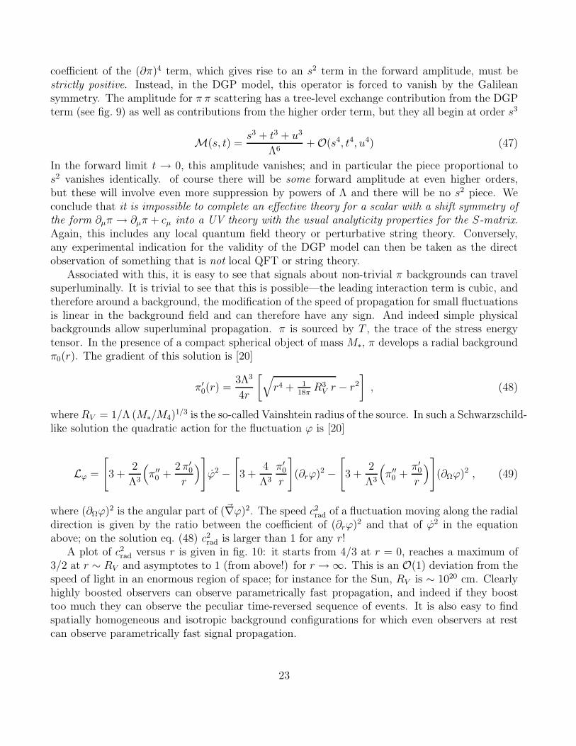
A plot of c2rad versus r is given in fig. 10: it starts from 4/3 at r = 0, reaches a maximum of3/2 at r ∼ RV and asymptotes to 1 (from above!) for r → ∞. This is an O(1) deviation from thespeed of light in an enormous region of space; for instance for the Sun, RV is ∼ 1020 cm. Clearlyhighly boosted observers can observe parametrically fast propagation, and indeed if they boosttoo much they can observe the peculiar time-reversed sequence of events. It is also easy to findspatially homogeneous and isotropic background configurations for which even observers at restcan observe parametrically fast signal propagation.

23

0.1 0.2 0.3 0.4 0.5 0.6r RV

0.20.40.60.8

11.21.41.6

crad2

Figure 10: The speed of radially moving fluctuations in a Schwarzschild-like solution in DGP.

Having found superluminal propagation, we run into the same paradoxes as we discussed insection 2. For instance two blobs of π field boosted towards each other in the x direction with asmall separation in y give rise to the same closed timelike curve problems as in the two boostedblob Goldstone examples. However, while there we assumed the presence of suitable sources thatcould give rise to our paradoxical field configuration, here we expect something more. Since thesimple Schwarzschild-like solution we just described features superluminal propagation, a closedtimelike curve should appear in the π field actually sourced by two masses boosted towards eachother. This is not easy to check: a quick estimate shows that in order to close the closed timelikecurve the two masses must pass so close to each other that, even if their Vainshtein regions donot overlap, the presence of one mass induces sizable non-linearities close to the other, and viceversa. In other words, the full solution is not just the linear superposition of two Schwarzschild-like solutions—new non-linear anisotropic corrections must be taken into account. It would beinteresting to further investigate such a configuration and understand whether a closed timelikecurve really arises.

It is instructive to contrast this with what happens for a generic Goldstone theory, wherethe leading interaction is still the same cubic term, but we also have the (∂π)4 terms. In thepresence of a generic background field π0(x) this interaction gives a contribution to the quadraticLagrangian for the fluctuations which is linear in the background,

δL =2

Λ3(∂µ∂νπ0 − ηµνπ0) ∂

µϕ∂νϕ . (50)

If we turn on a background with constant second derivatives, then the field equation for thefluctuation ϕ is exactly of the form eq. (10), with CµCν replaced by ∂µ∂νπ0. Exactly as inthe DGP analysis, it appears that superluminal signals are possible since ∂µ∂νπ0 has no a prioripositivity property. However the (∂π)4 term saves the day. We can certainly set up in some regiona background with constant ∂2π0 and negligible ∂π0, so that the effect of the cubic dominates overthat of (∂π)4; but this region cannot be larger than L ∼

√

Λ/∂2π0, since ∂π0 grows linearly withx for constant ∂2π0, and after a while the (∂π)4 term starts dominating the kinetic Lagrangian of

24

the fluctuations. Once this happens, if the coefficient of (∂π)4 is positive there are no superluminalexcitations.

The correction to the propagation speed inside the region where the cubic dominates is δc ∼∂2π0/Λ

3, so the maximum time advance/delay we can measure for a fluctuation traveling all acrossthe ‘superluminal region’ is

δtmax ∼ L δc ∼ ∂2π1/20

Λ5/2. (51)

Now, we would normally require ∂2π0 ≪ Λ3 in order for the effective theory to make sense. Insuch a case we immediately get δtmax ≪ 1/Λ, too small a time interval to be measured insidethe effective theory. However [20] argued that in a theory like eq. (42) consistent assumptionsabout the UV physics can be made to extend the regime of validity of the effective theory to muchlarger background fields and to much shorter length scales. In particular, in the presence of astrong background field ∂2π0 ≫ Λ3 the effective cutoff scale is raised from Λ to Λ ∼

√

∂2π0/Λ.In this case too the superluminal time advance is unmeasurably small: the size of the region inwhich the effect of the cubic dominates over the quartic is of order of the UV effective cutoff,L ∼

√

Λ/∂2π0 ∼ Λ−1. In both cases the quartic saves the day. Thus, not only does the coefficientof the (∂π)4 term have to be positive, it must be set by the same scale as the coefficient of thecubic term, a conclusion we could have also reached from the dispersion relation arguments of theprevious section.

We have uncovered a subtle inconsistency of the DGP model. As a classical theory, it haswell-defined, two-derivative, Lorentz invariant equations of motion; this property underlies thehealthy non-linear behavior of the theory and distinguishes it from more brutal modifications ofgravity, such as the theory of a massive graviton. However, just as in the simple scalar fieldtheory examples studied in the previous sections, which also have Lorentz invariant two-derivativeequations of motion, the theory suffers from a lack of a Lorentz-invariant notion of causality, whichis in turn related to a violation of the usual analyticity properties of scattering amplitudes.

Of course, even in brane models respecting the usual UV locality properties, there are DGPterms induced on the brane. What we have shown is that we can not have a decoupling limitwith M4/M5 → ∞ holding M2

5 /M4 fixed. This suggests that there is a limit of M4/M5 in anysensibly causal theory—it would be interesting to investigate these questions from the geometricalperspective of the five dimensional theory in more detail.

There is also an interesting connection between our constraint on the DGP model and the“weak gravity” conjecture of [9]. Both situations involve trying to make some interaction muchweaker than bulk gravity—in DGP it is the 4D Gravity on the brane, taking M4 ≫ M5, while in[9], it is the attempt to keep MP l and the cutoff of the theory fixed, but send 1/g2

4 → ∞. Wehave seen that a simple physical principle—requiring subluminal signal propagation—prohibitsthe DGP limit. Similarly, it appears that other general physical principles—such as the absenceof global symmetries in quantum gravity—block taking the weak coupling limit. In both cases,there are obstacles to making any interaction physically weaker than bulk gravity.

25

6 Positivity in the Chiral Lagrangian

There are similar positivity conditions in more familiar effective field theories in particle physics.Consider for instance the SU(2) chiral Lagrangian, parametrized by the unitary field U = eiπaσa

,

L = f 2 tr(∂µU†∂µU) + L4

[

tr(∂µU†∂µU)

]2+ L5

[

tr(∂µU†∂νU)

]2+ · · · (52)

There is a solution of the equations of motion with π pointing in a specifc isospin direction whichwe can take to be σ3, of the form

π3(x) = cµxµ (53)

We can look at the small fluctuations of both π3 as well as π± around this background. It is theneasy to check that in order for both π3 and π± to propagate subluminally we must have

L4,5 > 0 (54)

In our previous Abelian examples, the 4-derivative terms were the leading irrelevant interactionsin the theory, and so did not have any logarithmic scale dependence. On the other hand, L4,5

are logarithmically scale dependent; so the positivity constraint is then actually a constrainton the running couplings at energies parametrically smaller than Λ ∼ 4πf . Indeed, we canimagine turning on a background where ∂µπ

3 is approximately constant over a length scale Rmuch larger than the cutoff scale; in order to avoid superluminality we should demand that thatrunning L4,5 evaluated near this scale are positive. Of course, the log running of L4,5 inducedoff the lowest-order 2-derivative term pushes L4,5 positive, and so in a theory without a weak-coupling expansion, L4,5 at low-energies are dominated by the log running contribution and thereis no interesting constraint on the UV physics. However in theories with a weak coupling g, thematching contribution to L4,5 at the scale Λ will dominate over the log-running contribution downto energies of order Λe−1/g2

, and we can independently identify the matching contribution to L4,5

from the high-energy physics from the low-energy running contribution, and hence the positivitybound is a non-trivial constraint.

Naturally, the existence of these sorts of positivity constraints following from dispersion theoryare very well known, though not said very explicitly; our present example was discussed (thoughperhaps not widely recognized) in the literature long ago [24].

Of course the pion chiral Lagrangian follows from QCD which is a local quantum field theory,so these conditions must neccessarily be satisfied. The situation is perhaps more interestingfor the electroweak chiral Lagrangian governing the dynamics of the longitudinal components ofthe W/Z bosons. While it is most likely, given precision electroweak constraints, that the UVcompletion involves Higgses and a linear sigma model, there may also be more exotic possibilities,including in the extreme case a low fundamental scale close to the electroweak scale. This physicsshould manifest itself through the higher-dimension operators in the effective Lagrangian, andassuming custodial SU(2) is a good approximate symmetry, the constraint on the electroweakchiral Lagrangian is the same L4,5 > 0 (with the derivatives covariantized for the SU(2) × U(1)gauge symmetry ∂µ → Dµ). These operators are not associated with the well-known constraintsof precision electroweak physics— instead, in unitary gauge U = 1, they represent anomalousquartic couplings for the W/Z, which must be positive.

26

7 Examples from String Theory

7.1 Little String Theory

As we have seen, UV theories which are local or, what is the same, satisfy the usual analyticityproperties of S-matrix theory, give rise to effective theories with positivity constraints on certainleading irrelevant interactions that forbid superluminality and macroscopic non-locality. If weexperimentally measure such interactions and find that they are zero or negative, then we havedirect evidence for a fundamentally non-local theory. But if we also happen to know some ofthese operators theoretically, on other grounds, we can use them as a locality test for the UVcompletion.

The prime candidate for such a test is of course M-theory, which does not have a weaklycoupled description, and is thought by many to be fundamentally non-local. However, as we sawin the last section, in gravitational theories, there is no well-defined way to extract informationabout higher-dimension operators from superluminality constraints, since the notion of the correctmetric to use for the GR lightcone can be modified by higher-dimension operators, while justgravity already bends all signals inside the underlying Minkowski lightcone. Associated withthis, gravitational amplitudes are dominated by long-distance graviton exchange in the forwarddirection, with t-channel poles, and the dispersion relation arguments can’t be used.

However, we can certainly study non-gravitational UV completions of higher-dimensional gaugetheories, especially supersymmetric ones. In five dimensions, maximally supersymmetric Yang-Mills theories are UV completed into the six dimensional (2, 0) superconformal theory, whichalthough mysterious is still a local CFT. On the other hand, 6D super-Yang Mills is UV completedinto the 6D little string theory, which is a non-gravitational string theory with string tension setby the 6D Yang-Mills coupling but no small dimensionless coupling. This is another candidatefor a “non-local” theory. This issue can be probed if we can determine the coefficient of the F 4

operators in the low-energy SYM theory—if any of them have the “wrong” sign, this would provethat the LST is dramatically non-local.

Some of these F 4 terms have in fact been determined by a variety of methods. For instance,the U(N) theory has a Coulomb branch where it is Higgsed to U(1)N , and far out along theCoulomb branch, where the W ’s are much heavier than the little string scale, the F 4 couplingbetween the U(1)’s have been computed [21]. They are all positive. This is perhaps not surprising,since they are related by dualities to F 4 coefficients in weakly coupled theories where the signsare determined. Thus, if LST is really non-local, the non-locality did not put in an appearance inthe F 4 terms.

7.2 Non-commutative theories

Probably the best studied example of the Lorentz-violating system in string theory is a stack ofparallel D-branes in flat space-time with constant non-zero value of antisymmetric tensor fieldBµν along the brane world-volume. It is instructive to see how superluminality constraints workin this case. In the presence of non-zero Bµν open string modes localized on D-branes propagate

27

in the effective metric Gµν related to the closed string metric ηµν in the following way [22],

Gµν = ηµν − (2πα′)2BµλBλν . (55)

The metric Gµν is a direct analogue of the effective metric discussed in sect. 3.2, so we expect itscausal cone to be contained in the light cone of the Minkowski metric. To check this let us pick upan arbitrary light-like vector nµ = (1, ni) and calculate its norm with respect to the open stringmetric Gµν . One finds

nµGµνnν = −(Ei − niEjn

j − Bijnj)2

where Ei = B0i. Consequently, nµ is either space-like or null with respect to the open stringmetric, implying that its causal cone is indeed contained in the usual light cone. Note that thisconclusion holds not only for small values of Bµν , but in the presence of strong field as well. Forthe background of the electric type one should of course require that the electric field is smallerthan the critical value when metric Gµν changes its singature. Physically at this point vacuumbecomes unstable towards pair production of massive charged string modes.

In the limit of large magnetic field the propagation velocity of open modes vanishes as comparedto the speed of closed modes. In this limit closed strings decouple from open modes and dynamicsof the open sector is described by the non-commutative field theory. At the classical level thistheory exhibits approximate Lorentz-invariance (with open string metric playing the role of theLorentz metric) which is broken by the higher-dimensional operators proportional to the non-commutativity parameter. Interestingly, these theories allow soliton solutions which can propagatefaster than the speed of “light” as defined by the open string metric Gµν [23]. This fact however,neither contradicts to our superluminality constraints nor leads to any problems with causalitybecause these solitons still propagate inside light cone of the closed string metric which is the trueLorentz metric of the underlying theory.

8 Gravity

So far, we have been discussing non-gravitational theories. In a theory with gravity, there is anatural UV cutoff scale of order MP l, and it is natural to ask whether there are constraints on1/MP l suppressed operators from our considerations.

It is easy to see that there can’t be any straightforward analog of our superluminality con-straints in GR. The reason is that in a gravitational theory, it is natural to define the light-coneby gµν . The effect of any higher dimension operator on the GR lightcone can then completely beabsorbed into a redefinition of the metric by 1/MP l suppressed operators. There is also no analogof our arguments using the vanishing of commutators of local operators outside the light-cone.There are no local gauge invariant operators in gravity—one of the reasons the only observable ina quantum theory of gravity in flat space is the S-matrix.

However, we might take another track. For weak enough gravitational fields we can certainlythink of General Relativity as a Lorentz invariant theory of a spin-2 field interacting with matterfields in Minkowski space. The underlying Minkowski space has a metric ηµν and a well definedlight-cone, which we shall refer to as the “Minkowski light-cone”. On the other hand a classical

28

gravitational field defines a new light-cone, the cone of null geodesics of the full metric gµν irra-diating from a point; we call this the “gravity light-cone”. In the weak field approximation weare considering, the fact that massless particles propagate along the gravity light-cone takes intoaccount the interaction of these particles with the background gravitational field. This is verysimilar to what we have been discussing so far, the propagation of signals in a Lorentz-violatingbackground field. Indeed we can ask whether it is possible to turn on a gravitational field suchthat the Minkowski light-cone lies inside the gravity one, so that massless excitations, interact-ing with the background gravitational field, can actually travel outside the underlying Minkowskilight-cone.

At first this seems to be trivially possible, since the effect the gravitational field has on thedispersion relation of a massless particle is linear in the background field itself, and as such it hasno a priori definite sign. In fact in the geometric optics limit the dispersion relation is simply thestatement that the particle wave-vector kµ is null with respect to the full metric gµν = ηµν + hµν ,

(ηµν − hµν) kµkν = 0 . (56)

If hµν is not a negative-definite matrix, then there exists a kµ obeying the above equation thatis time-like with respect to the underlying Minkowski metric, which means that the particlecan travel outside the Minkowski light-cone. For instance a plane gravitational wave has a nonnegative-definite hµν .

However we must wonder how we actually set up the background gravitational field. For solvingEinstein’s equations we need to fix the gauge. Since we want to preserve Lorentz invariance, wechoose De Donder gauge, ∂µ(hµν − 1

2h ηµν) = 0. Einstein’s equations then read

(hµν − 12h ηµν) = −16πGTµν , (57)

where Tµν is the sources’ stress-energy tensor. Outside the sources we can further constrain thegauge by setting h = 0. The retarded gravitational field ouside the sources is therefore

hµν(t,x) = −4G

∫

d3r1

rTµν(t− r,x + r) . (58)

Now it is clear that hµν kµkν can be made positive only if Tµν k

µkν is negative somewhere, but thisis in contradiction with the Null Energy Condition. Notice that a violation of the Null EnergyCondition under very broad assumptions leads either to instabilities at arbitrarily short time-scalesor to superluminal propagation in the matter sector [12]. The negativity of hµν physically meansthat even if gravitational waves are present, the contribution of the static Newtonian potential tohµν due to the very same sources that emitted the gravitational waves is always larger than theoscillatory one, and negative definite.4

We are therefore led to the conclusion that, in the weak field approximation we are in, it isimpossible to set up a gravitational field such that null geodesics move outside the underlyingMinkowski light-cone. Gravity ‘bends’ all null trajectories inside the Minkowski light-cone. Thisconclusion was also reached a number of years ago in [25].

4At first this seems to contradict the usual fact that far from the source the wave field decays slower than thestatic one. This is indeed true at the level of field-strenghts, but the potentials themselves both decay like 1/r.

29

This is a satisfying result. However, it also makes it impossible to constrain higher-dimensionoperators using superluminality arguments—since the Einstein action already pushed signals insidethe Minkowski light-cone, higher-order operators can’t change this conclusion regardless of theirsign.

The difficulty of bounding higher-dimension operators suppressed by MP l is also apparent indiscussing 2 → 2 scattering amplitudes. From our previous experience, it is evident that thereare positivity constraints on 2 → 2 scattering in the forward direction t → 0. However, in agravitational theory, already at tree-level, massless 1-graviton exchange dominates the 2 → 2scattering amplitude as t→ 0,

M(s, t) ∼ GNs2

t, (59)

so again, the effect of any higher order operators are swamped by the lowest order massless 1-graviton exchange which dramatically violated the Froissart bound.

In the context of a UV theory with a weak-coupling factor, however, there is some hope.For instance, consider weakly coupled string theory, and consider the amplitude for masslessclosed string mode scattering. The lowest order tree amplitude has a contribution from gravitonexchange, as well as from the tower of Regge states. We can isolate the contribution from Reggestates simply by subtracting the tree-level graviton exchange diagram. The resulting subtractedamplitude then has a well-behaved limit as t→ 0. On the other hand, the Regge behavior of thefull amplitude as s → ∞ for fixed t tells us that the amplitude behaves as sα(t)/t at large s, andtherefore, upon subtracting the tree-level graviton contribution that removes the t-channel pole,the amplitude is polynomially bounded in the complex s plane. Thus, we should expect that ast→ 0 the leading amplitude is of the form

M(s, t) → GNs2

t+ polynomial in s2 with all positive coefficients , (60)

which again implies an infinite number of constraints on the coefficients of higher-dimension op-erators in the theory.

Let us see how this works explicitly for the scattering of NS-NS bosons of type II strings in 10dimensions. The full scattering amplitude is of the form

M(s, t, u) = −g2s

4K

Γ(−14s)Γ(−1

4t)Γ(−1

4u)

Γ(1 + 14s)Γ(1 + 1

4t)Γ(1 + 1

4u)

(61)

where once again K is a factor depending on external polarizations; for our purposes it is onlyimportant that as t→ 0, K ∼ s4. The amplitude can be expanded as

M = Mgrav + MRegge , (62)

where

Mgrav = −64K

s t u(63)

is the tree-level graviton contribution, while MRegge is by definition the contribution to the tree-level amplitude from the heavy Regge modes. Of course MRegge has a good behavior as t → 0,

30

and it is easy to check that it is indeed polynomially bounded at infinity; in fact it is bounded by|s|4 at large s. From our general argument, all the terms beginning with s4 are guaranteed to bepositive, and indeed

MRegge(s, t→ 0) = −ψ2(1) s4 +−ψ4(1)

192s6 +

−ψ6(1)

92160s8 + . . . (64)

where all the polygamma functions ψn(1) are negative.Thus, while we can’t say anything in general about higher-order operators in gravitational

theories, there is a simple diagnostic for whether certain gravitational amplitudes do not comefrom a weakly coupled string theory—if the short-distance contribution to the amplitide is apolynomial in s2 with any negative coefficients, it can’t come from a perturbative closed stringmodel.

9 Discussion

We have shown that certain apparently consistent effective field theories described by local,Lorentz-invariant Lagrangians are secretely non-local. The low-energy manifestation of this lurk-ing non-locality is the possibility of superluminal signal propagation around coherent backgroundfields. This creates a tension between causality and Lorentz-invariance: in such theories noLorentz-invariant notion of causality or locality exists. The high-energy face of this tension isthat such theories can not be UV completed into full theories that satisfy the usual axioms ofS-matrix theory, specifically the analyticity conditions that encode locality. Both local quantumfield theories and string theories satisfy these properties, so we have provided a simple diagnosticfor theories that can not be embedded into local QFT’s and string theory.

In effective theories where the particle content or symmetries force the leading interactions to beirrelevant operators, completely standard dispersion-relation arguments force positivity conditionsin these interactions. In terms of the scattering amplitude, the coefficient of the leading s2 termin the forward amplitude must be strictly positive. This requirement precisely guarantees theabsence of superluminal excitations around coherent backgrounds. In weakly coupled theories,there is the stronger constraint that the leading amplitude is a power series in s2 with all positivecoefficients.

Our analysis applies to the DGP model—specifically the four-dimensional effective theory forthe “brane-bending” mode π that is all that is left in a decoupling limit sending M4,M5 → ∞keeping Λ = M2

5 /M4 fixed. This scalar theory is controlled by a nice symmetry—interpreted asGalilean invariance in the underlying 5D theory, under which ∂µπ → ∂µπ + cµ. This symmetryforces the coefficient of the leading operator giving rise to an amplitude proportional to s2 to vanish,in contradiction to the strict positivity of this coefficient in any UV local theory. Associated withthis, signals about consistent π backgrounds can propagate parametrically faster than light.

Similar considerations apply to the chiral Lagrangian, where the coefficient of some of the4-derivative terms are forced to be positive. In the electroweak chiral Lagrangian, these turn intoanomalous W/Z quartic gauge couplings in unitary gauge. Thus, UV locality implies that suchanomalous couplings are necessarily positive.

31

All of our considerations in this paper have concerned Lorentz-invariant theories with a Lorentz-invariant ground state. It is the presence of the asymptotic Minkowski space that allows us to getinto paradoxes involving highly boosted bubbles. While our arguments do not directly apply totheories in which the vacuum spontaneously breaks Lorentz invariance, such as Higgs phases ofgravity [6, 7, 8] or the models studied in [12], it would be interesting to ask whether there are anyanalogous constraints to those we have discussed.

The UV face of the positivity constraints we have described are of course implicitly well-knownin dispersion theory. In the context of the chiral Lagrangian, precisely the positivity constraintswe describe have been discussed for instance in [24]. However, the directness with which theseimportant signs pinpoint effective theories that can or can not arise from local UV theories, andthe connection with superluminality and the breakdown of macroscopic locality, has not beenappreciated. For instance, any experimental support for the DGP model, or negative signs foranomalous quartic gauge boson couplings, can be taken as a direct indication of the existence ofmacroscopically non-local physics unlike anything ever seen in physics, either in quantum fieldtheory or weakly coupled string theory. Experimental tests of positivity then provide a powerfulprobe into the validity of some of our most firmly held assumptions about fundamental physics.

Note that our results are quite likely to have interesting connections to the physics of horizons.For example, in theories violating positivity, a Rindler observer immersed in the translation-ally invariant superluminal background can see behind the nominal Rindler horizon to see allof Minkowski space. Similarly, it should be possible to see behind black hole and cosmologicalhorizons by tossing superluminal bubbles at them, which runs afoul of all the usual rules abouthorizons and their thermodynamic properties. Another concrete link between positivity and black-hole physics was developed in [9]. It would be interesting to further explore such connections.

Similarly, it would be interesting to apply positivity to various models under considerationto identify which can be embedded in local UV theories, and which are in fact fundamentallynon-local. Obvious candidates are various beyond-the-standard-models with leading derivativeinteractions, as well as the host of interesting varying speed-of-light models of interest in cosmology,many of which very likely run afoul of positivity.

More generally, we have studied only one very simple constraint on the low-energy effectivefield theory of a local, Lorentz-invariant UV-complete Quantum Field Theory deriving from theanalyticity of the UV S-matrix, namely, positivity of forward 2 → 2 bosonic scattering ampli-tudes. For example, it would be interesting to identify constraints deriving from higher scatteringamplitudes, amplitudes involving fermions, gravitational amplitudes, etc. It would also be inter-esting to identify other properties of UV-complete models above and beyond simple analyticity ofthe S-matrix—do they lead to interesting constraints on which effective field theories may be UVcompleted, and if so, what is the IR pathology of a theory which runs afoul of such a constraint?It seems possible that there are many more constraints on just which effective theories may beconsistently embedded in UV-complete theories, and, in particular, string theory.

Acknowledgements

We would like to thank Paolo Creminelli, Oliver DeWolfe, Jacques Distler, Gia Dvali, GregoryGabadadze, Leonardo Giusti, Thomas Gregoire, Shamit Kachru, Markus Luty, Aaron Pierce,Massimo Porrati, Valery Rubakov, Leonardo Senatore, Misha Shifman, Raman Sundrum, Sergei

32

Sibiryakov, Igor Tkachev, Enrico Trincherini, and Arkady Vainshtein for helpful conversationsabout these ideas. A. A. would particularly like to thank Aaron Pierce for invaluable assistanceduring the final revisions of this note. We thank Howard Schnitzer for pointing out elementarilyincorrect things about the analytic structure of amplitudes said in the first version of this paper,and for a helpful conversation about it. N. A.-H. would like to thank Lubos Motl and especiallyMichal Fabinger for deconfusing him with extremely helpful and illuminating discussions. Thework of N. A.-H. is supported by the DOE under contract DE-FG02-91ER40654. The work ofA. A. is supported by a Junior Fellowship from the Harvard Society of Fellows. The work of R. Ris partly supported by the European Commission under contract MRTN-CT-2004-503369.

References

[1] S. Kachru, R. Kallosh, A. Linde and S. P. Trivedi, “De Sitter vacua in string theory,” Phys.Rev. D 68, 046005 (2003) [arXiv:hep-th/0301240].

[2] S. Weinberg, “Anthropic Bound On The Cosmological Constant,” Phys. Rev. Lett. 59, 2607(1987).

[3] V. Agrawal, S. M. Barr, J. F. Donoghue and D. Seckel, “The anthropic principle and themass scale of the standard model,” Phys. Rev. D 57, 5480 (1998) [arXiv:hep-ph/9707380].

[4] N. Arkani-Hamed and S. Dimopoulos, “Supersymmetric unification without low energysupersymmetry and signatures for fine-tuning at the LHC,” JHEP 0506, 073 (2005)[arXiv:hep-th/0405159]; G. F. Giudice and A. Romanino, “Split supersymmetry,” Nucl. Phys.B 699, 65 (2004) [Erratum-ibid. B 706, 65 (2005)]; N. Arkani-Hamed, S. Dimopoulos andS. Kachru, “Predictive landscapes and new physics at a TeV,” arXiv:hep-th/0501082.

[5] G. R. Dvali, G. Gabadadze and M. Porrati, “4D gravity on a brane in 5D Minkowski space,”Phys. Lett. B 485, 208 (2000), [arXiv:hep-th/0005016].

[6] N. Arkani-Hamed, H. C. Cheng, M. A. Luty and S. Mukohyama, “Ghost condensation and aconsistent infrared modification of gravity,” JHEP 0405, 074 (2004), [arXiv:hep-th/0312099].

[7] V. A. Rubakov, “Lorentz-violating graviton masses: Getting around ghosts, low strong cou-pling scale and VDVZ discontinuity,” arXiv:hep-th/0407104.

[8] S. L. Dubovsky, “Phases of massive gravity,” JHEP 0410, 076 (2004) [arXiv:hep-th/0409124].

[9] N. Arkani-Hamed, L. Motl, A. Nicolis and C. Vafa, “The string landscape, black holes andgravity as the weakest force,” arXiv:hep-th/0601001.

[10] C. Vafa, “The string landscape and the swampland,” arXiv:hep-th/0509212.

[11] G. Dvali, A. Gruzinov and M. Zaldarriaga, “The accelerated universe and the Moon,” Phys.Rev. D 68, 024012 (2003) [arXiv:hep-ph/0212069].

33

[12] S. Dubovsky, T. Gregoire, A. Nicolis and R. Rattazzi, “Null Energy Condition and Superlu-minal Propagation,” arXiv:hep-th/0512260.

[13] R. M. Wald, General Relativity, The University of Chicago Press, 1984.

[14] J. Polchinski, String theory. Vol. 2: Superstring theory and beyond.

[15] M. Froissart, “Asymptotic Behavior And Subtractions In The Mandelstam Representation,”Phys. Rev. 123, 1053 (1961).

[16] A. Martin, “Unitarity And High-Energy Behavior Of Scattering Amplitudes,” Phys. Rev.129, 1432 (1963).

[17] N. Arkani-Hamed, H. Georgi and M. D. Schwartz, “Effective field theory for massive gravitonsand gravity in theory space,” Annals Phys. 305, 96 (2003), [arXiv:hep-th/0210184].

[18] M. A. Luty, M. Porrati and R. Rattazzi, “Strong interactions and stability in the DGPmodel,” JHEP 0309, 029 (2003), [arXiv:hep-th/0303116].

[19] D. Gorbunov, K. Koyama and S. Sibiryakov, “More on ghosts in DGP model,”arXiv:hep-th/0512097.

[20] A. Nicolis and R. Rattazzi, “Classical and quantum consistency of the DGP model,” JHEP0406, 059 (2004), [arXiv:hep-th/0404159].

[21] O. Aharony, B. Fiol, D. Kutasov and D. A. Sahakyan, “Little string theory and heterotic/typeII duality,” Nucl. Phys. B 679, 3 (2004) [arXiv:hep-th/0310197].

[22] N. Seiberg and E. Witten, JHEP 9909, 032 (1999) [arXiv:hep-th/9908142].

[23] A. Hashimoto and N. Itzhaki, Phys. Rev. D 63, 126004 (2001) [arXiv:hep-th/0012093].

[24] T. N. Pham and T. N. Truong, “Evaluation Of The Derivative Quartic Terms Of The MesonChiral Lagrangian From Forward Dispersion Relation,” Phys. Rev. D 31, 3027 (1985).

[25] M. Visser, B. Bassett and S. Liberati, “Superluminal censorship,” Nucl. Phys. Proc. Suppl.88, 267 (2000) [arXiv:gr-qc/9810026].

34