CAV2001:lecture.001 1

Abstract Scale effects on cavitation phenomena are departures from the classical relation due to variations in

a) water quality with regard to its cavitation susceptibility (tensile strength, concentration and size of nuclei)

b) body size and flow parameters (flow velocity, viscosity of the fluid, turbulence). These scale effects are an important consideration in the prediction of the prototype cavitation behaviour

based on model tests. Test results show that, provided effects of water quality are avoided in the experiments, very clear empirical relations can be established for the scale effects on cavitation inception. The data, on which these empirical relations are based, relate to the inception of various types of cavitation as they occur on the surface of rotationally symmetric bodies, two-dimensional non lift producing bodies, or two- and three-dimensional lift producing foils. It can be shown, that the scaling relations initially found for beginning cavitation also are valid for developed cavitation. In addition lift and/or drag forces were measured on all kinds of test bodies and correlated with the cavitation number, and good correlation is obtained between the cavitation parameter and the corresponding measured drag coefficient. The new findings about the correlation of cavitation numbers with drag coefficients are believed to be the clue to why the empirically found scaling relations are so universal, and a key to the physical explanation for these scale effects.

1 Introduction The cavitation phenomenon has received widespread attention and intense investigation in many fields of

engineering, ranging from aerospace to civil engineering, from ship building to turbine and pump industry. Although the occurrence of scale effects with model tests has long been well known and was already mentioned 1930 by Ackeret, it can be stated, that there is no generally accepted similarity law, neither for the transfer of model test results to the prototype, nor even for test results of identical or similar model bodies investigated in different test facilities. As early as 1963 the Cavitation Committee of the ITTC initiated a comparative test program related to cavitation inception on head forms. The results were widely scattered in that an increase of velocity lead to decreasing, constant or increasing cavitation indices.

Later, extensive comparative tests in the 70-ies on hydrofoils were initiated by the ITTC. The aim of the test program was to determine inception of different types of cavitation as a function of tunnel water speed and gas content ratio. Again the data showed large differences between the various tunnels and observers. Figure 1 shows the dilemma of incomparability of test results. It is one example of many that can be found in the literature. Large differences in inception number and its velocity dependency are found between the tunnels involved (ITTC 1978).

Many summaries of this problem are available in the literature, and it is not the intent of this paper to provide yet another review. However, an attempt will be made to document the complexity of the scale effects, and to show the state of development of scaling relations, which were evaluated from long series of cavitation tests on different test body families at the hydraulic laboratory in Obernach.

CAVITATION SCALE EFFECTS EMPIRICALLY FOUND RELATIONS AND THE CORRELATION

OF CAVITATION NUMBER AND HYDRODYNAMIC COEFFICIENTS

Andreas P. Keller Institute of Hydraulic and Water Resources Engineering,

Technische Universität München, Germany

brought to you by COREView metadata, citation and similar papers at core.ac.uk

provided by CaltechCONF

CAV2001:lecture.001 2

2 The Classical Cavitation Index and Water Quality Effects Prediction of cavitation performance on all kinds of submerged bodies and hydraulic machinery is derived

from model tests in cavitation test facilities. For estimation of the danger of cavitation of hydraulic machines, such as pumps and turbines, elements of ships, or hydraulic structures in civil engineering, the beginning and subsequent development of cavitation phenomena are evaluated experimentally. The submerged parts are investigated as models in a test facility where its cavitation behavior is judged. The key parameter, which is used usually, is the dimensionless cavitation index

22

1 ∞

−∞=

VVPP

ρσ (1)

wherein P∞ and V∞ are a characteristic pressure and velocity of the flow upstream of the body, ρ and PV represent the density and vapor pressure of the liquid, respectively.

0,0

0,2

0,4

0,6

0,8

1,0

1,2

1,4

1,6

1,8

2,0

2,2

4 5 6 7 8 9 10 11V

���� [m/s]

σσσσ

SSPA 2

PARIS

SSPA 1

NSMB

TUB

NSMB

PARISHYDR

INTERMITTENTPERMANENT

0,0

0,1

0,2

0,3

0,4

0,5

0,6

0,7

0,8

0,9

6 8 10 12 14 16 18 20V

���� [m/s]

σσσσ

VAO LCC ARL

12,7 mm

25,4 mm

50,8 mm508 mm

254 mm

50,8 mm

60 mm

30 mm

15 mm

Figure 1: Example of the dilemma of incomparability of test results, demonstrated at one and the same test body, investigated in different test facilities (ITTC 1978)

Figure 2: Traditional cavitation number versus flow velocity of VAO, LCC and ARL data

The cavitation theory assumes, that the cavitation phenomena at the model and the prototype for geometrically similar bodies are identical at equal σ-values, irrespective of variations in physical parameters like body size, flow velocity, temperature, type of the liquid, etc. One particularly important value of σσσσ is the value at which cavitation is first observed, for this cavitation condition is definable the most precisely. All conditions beyond this must be denoted as developed cavitation, and are not repeatable precisely for another observer. The difficulty of reproducing cavitation inception at one test body in different test facilities, is pointed out by the wide scatter of comparable results in the literature (see Figure 1).

From systematic investigations and experience in practice it is well known, that the classical cavitation relation (1) allows no sufficiently precise transfer of test results from the model to the prototype. At a submerged part of a prototype fully developed cavitation is visible, whilst at its model at identical cavitation number no or just beginning cavitation can be observed. Also, at identical test bodies, differently marked cavitation is observable if they are exposed to different velocities at equal σ-values. Differences in the viscosity of the fluid

CAV2001:lecture.001 3

and the turbulence level of the flow have possibly additional strong effects on the extension of cavitation . These differences in the cavitation phenomena at model and prototype, or at one test body at equal σ but different flow parameters, are summarized under the term "scale effects".

In order to demonstrate this, test results carried through at two different test facilities are compared in Figure 2. One set of data shows the results of cavitation inception tests on three body sizes of the so-called Schiebe body of 75.0min =PC , carried out in a most modern test facility , i.e. the LCC of the US Navy (Kuhn et al. 1992), whilst in the second dataset the results at three other test bodies of the same body contour, carried out at the ARL (Holl et al 1987), are plotted. Both results show a distinct size scale effect, however, while the LCC-data show decreasing values for the cavitation number with increasing flow velocity, the ARL- data show the opposite trend.

Basic supposition with cavitation investigations is, that the rupture of liquids begins when the pressure in the flow around a submerged body reaches vapor pressure, PV, as equation (1) implies. The fact that cavitation tests at identical test bodies, or even the same test body, carried out in different test facilities lead to totally different results proves this assumption to be valid only as the exception. This wide scatter of experimental results can be attributed primarily to different tensile strength, Pts, of the test liquid, i.e. to different water quality concerning its cavitation susceptibility.

In Figure 3 the cavitation phenomena at the tip of a profile (NACA 16 020, angle of attack 6°) are shown for three different water qualities at equal cavitation number (σ = = = = 0.69) and equal flow velocity (V∞ = 9.5 m/s). In the first photo no cavitation is visible at high tensile strength of the test water. In the second photo, for a water quality of zero tensile strength, beginning tip vortex cavitation can be recognized. A fixed cavity, caused by a surface irregularity is also visible. For negative tensile strength of the test water, a fully developed tip vortex cavitation and single bubble cavitation at the profile is registered.

a) High tensile strength of the test water; no cavitation

b) Zero tensile strength of the test water; beginning tip vortex cavitation

c) Negative tensile strength of the test water; traveling bubble and developed tip vortex cavitation

Figure 3: Effect of the water quality on the cavitation appearance for the example of a NACA 16020 profile (chord 200mm, α = 6°); V∞= 9,50 m/s, σ = 0,69 (flow is for all figures from left to right)

An example of extremely different appearances of tip vortex cavitation inception for varying water qualities is shown in the two following series of high speed video recordings. In the Figure 4 i.e. at zero tensile strength of the test water, cavitation starts at σ = 2.02 very close to the tip. After inception the cavitation bubble grows rapidly while moving downstream and being swept away from the tip.

In Figure 5, i.e. high tensile strength of the test water, at σ = 0.93 first sheet cavitation occurs at the suction side of the foil; no cavitation in the tip vortex. The liquid in the vortex core bears a high tension at this moment. Finally, after the sheet cavitation has developed, vortex cavitation starts rather far downstream from the tip, after either a nucleus of critical size was entrained from the flow into the vortex core, or a nucleus has grown by turbulent diffusion to critical size inside the over saturated core. Now the bubble grows rapidly and the cavitating core progresses upstream until it reaches the tip, and forms a stable vapor filled core which does not disappear anymore.

The wide range of scatter of experimental results can be attributed primarily to different tensile strength, Pts, of the test liquid, i.e. to different water qualities concerning its cavitation susceptibility. Figure 3 illustrates this fact.

The number for beginning cavitation, σi, can be made free of water quality effects, by replacing vapor pressure, Pv, by the actual critical pressure for rupture of the liquid, Pcrit = Pv - Pts.

CAV2001:lecture.001 4

tsitsVcrit

iV

PPPVPP

σ∆σρρ

σ +=+−

=−

=′∞

∞

∞

∞

22

21

21

(2)

Incipient tip vortex cavitation cl

Expanding cavitation in the tip v

Cavitating tip vortex floating do

Figure 4: Incipient cavitation at a modhydrofoil at α-α0=70, 10 m/s, tensile strength of the test watframes /s As shown in Figure 6 schematiessential. Whereas ∆σ for a givelocity, and tends theoreticallycurves asymptotically approachincreasing σi with increasing flo

A set of curves for cavitaticontents of the test water is shbehavior as the theoretical curvas the theoretical curve for negathen increasing σi. Beyond a ccurves for very low gas contentcontents with increasing velocitof zero tensile strength in Figure

Fr.No. 0001

ose to the tip Beginning sheet cavitation

Fr.No. 0050

ortex Developed sheet cavitation

5

Fr.No. 017

wnstream Beginning vortex cavitation down

Tip vortex cavitation expanding u

Cavitating vortex touching the tip

ified NACA 4215 σ = 2.02, and zero er; rec. rate 18.000

Figure 5: Incipient cavitation at a modifhydrofoil at α-α0=70, 10 m/s, σtensile strength, recording rate 18

cally, the effect of the tensile strength, Pts, of a liquid for caven Pts is relatively small for high velocities, it grows rap towards infinity when approaching zero velocity. With inc

the curve for zero tensile strength, and then follow the velow velocity (for definition of the velocity scaling law see later

on inception versus throat velocity in a 1/2 inch plexiglas venown in Figure 7 (Hammitt, 1980). These curves disclose

es in Figure 6. The curves for water with high gas content foltive tensile strength in Figure 6, i.e. first decreasing σi with

ertain velocity σi is only increasing for all gas contents, an show negative σ-values at low velocities and approach the cy; the curve for a gas content of 0.5 % corresponds roughly t 6.

Fr.No. -2200

Fr.No. -1900

Fr.No. -1665

stream of the tip

Fr.No.-1615

pstream

1

Fr.No. 000

ied NACA 4215 = 0.93, and high .000 frames/s

vitation tests can be idly with decreasing reasing velocity the city scaling law, i.e. ). turi for different gas a stunningly similar low the same course increasing velocity, d ∆σi is small. The urves for higher gas

o the curve for water

CAV2001:lecture.001 5

-1,0

0,0

1,0

2,0

3,0

4,0

0 5 10 15 20V

���� [m/s]

σσσσ

negativetensile strength

zerotensile strength

positivetensile strength

∆ σ ∆ σ ∆ σ ∆ σ

Figure 6: Schematically represented test results for cavitation inception with and without tensile strength of the test liquid

Figure 7: Cavitation inception number versus throat velocity for a 1/2 inch venturi for several gas contents in the test water (Hammitt, 1980)

The results shown in the photo series, as well as the test results with different water qualities imply that cavitation phenomena are extremely sensitive to water quality. This explains the tremendous scatter of results in comparable tests. Even small differences in water quality can lead to big differences in cavitation inception number. Thus water quality effects can lead to confusing results at cavitation tests, and this effect can outweigh real scale effects in cavitation tests, thus leading to totally wrong conclusions concerning the process for rationally extrapolating model data to estimates of prototype cavitation behavior of any given facility.

Therefore a measurement technique to determine the tensile strength of the test liquid was developed to its routinely applicable form, and used throughout the test program for the evaluation of the real scale effects. Details of this technique (Vortex Nozzle Chamber, VNC) as a cavitation susceptibility meter are already published, and will not be dealt with here (Keller 1981 and 1984).

3 The Empirically Found Hydrodynamic Scale Effects At the Institute of Hydraulic and Water Resources Engineering of the Technische Universität München in

Obernach numerous experiments on cavitation inception, under strict control of the water quality concerning its cavitation susceptibility, have been carried out on all kinds of bodies with regard to their shape and size, in different liquids with respect to their viscosity, and in oncoming flow of different turbulence level. The results of these tests pointed out that - the influence of the quality of the test liquid to the test results can be avoided if the tests are carried through

with nuclei saturated liquids (Pts = 0), and - the comparison of test results of different liquids is possible, if the cavitation number is calculated with the

measured critical pressure Pcrit = Pv - Pts, instead of the vapor pressure. and they revealed surprisingly clear relationships concerning the hydrodynamic aspects of scale effects.

CAV2001:lecture.001 6

3.1 The visual appearance of scale effects

3.1.1 Velocity scale effect

The following Figure 8 displays the velocity scale effect, meaning the appearance of cavitation at a submerged body at constant cavitation number σ for different flow velocities. The water quality concerning its cavitation susceptibility was held constant at zero tensile strength throughout the tests.

a) beginning cavitation at σ = 0.80 und V∞ = 8,0 m/s b) developed cavitation at σ = 0.80 und V∞ = 14,0

m/s Figure 8: Velocity scale effect on a hemispherical body

Whilst at the respective lowest flow velocities just beginning cavitation can be recognized, at higher velocities distinctly further developed cavitation is observable at constant σσσσ. The degree to which this obvious scale effect is in contradiction to the classical theory, is demonstrated by means of the principle representation of the velocity scale effect in Figure 9. Usually it is assumed that with changing velocity the cavitation appearance remains unchanged, if the σ-value is kept constant. However, as the photo series show, at higher velocities considerably developed cavitation is registered. In order to achieve the condition of beginning cavitation for the higher velocities, the static pressure must be raised, i.e. the σ-value must be increased by a respective ∆σ. The regression line through the experimental data point for cavitation inception is explained further down.

0

0,2

0,4

0,6

0,8

1

1,2

0 2 4 6 8 10 12 14

V���� [m/s]

σσσσ

Figure 9: Principle representation of the velocity scale effect shown with the example of the hemispherical body (30mm diameter)

CAV2001:lecture.001 7

3.1.2 Size scale effect

The following Figure 10 shows the size scale effect, i.e. the appearance of cavitation at three model bodies of identical form but of different size. Again the test conditions are equal cavitation number, and this time even equal flow velocity. Whilst at the respective smallest model just beginning cavitation can be recognized, with increasing body size distinctly further developed cavitation is visible.

The size scale effect is schematically illustrated in Figure 11. It is as well in contradiction to what is expected according to the classical theory. Usually it is assumed that at the larger models for the cavitation number corresponding to the cavitation inception number of the small model, just beginning cavitation is also to be observed. However, as the photo series show, at the larger models considerably developed cavitation is registered. In order to achieve the condition of beginning cavitation for the bigger model bodies at the same velocity, again the static pressure must be raised, i.e. the σ-value must be increased respectively.

a) max. chord length 50 mm σ = 2,18; V∞ = 11,0 m/s beginning tip vortex cavitation

b) max. chord length 100 mm σ = 2,18; V∞ = 11,0 m/s developed cavitation

c) max. chord length 200 mm σ = 2,18; V∞ = 11,0 m/s fully developed cavitation

Figure 10: Size scale effect for cavitation shown with the example of a NACA 16020 hydrofoil

The supposition shown in Figure 11 that σ, or σ0 (explained further down), respectively, become zero irrespective of body shape, when the size of the test body converges to zero, appears acceptable, if one considers the fact, that at that point there is no difference anymore between the body shapes, no boundary layer can develop in the flow, etc.

0,0

0,5

1,0

1,5

2,0

2,5

3,0

3,5

4,0

0 50 100 150 200L [mm]

σσσσ

Figure 11: Principle representation of the size scale effect shown with the example of the NACA 16020 hydrofoil

CAV2001:lecture.001 8

3.2 The empirically evaluated relations for the scale effects None of the parameters of influence represented above is taken into consideration in the classical

relationship for cavitation given by equ. (1). In the past years these parameters and their scale effects were investigated in long lasting test series in Obernach. By focusing on the parameter of influence generally blurring experimental results, i.e. the tensile strength of the liquid, clear dependencies for size, velocity, viscosity and turbulence scale effects were revealed, and it was proven, that cavitation tests performed without consideration of the "water quality" on cavitation susceptibility do not lead to useful and comparable results. Experimental results obtained with water quality considered, show a surprisingly clear regularity with regard to the real scale effects.

As a summary, a representative selection of the results of all previously tested bodies are displayed in Figure 12. The classical cavitation number σσσσ for incipient cavitation is plotted versus the flow velocity V∞ irrespective of shape, size, and liquid viscosity, the data points for all test bodies, connected by curves, show a steady increase of the σσσσ-number with increasing velocity. The curves start from a basic σ-value, σ0, for the reference velocity V∞ = 0. Altogether there appears a striking regularity in the set of curves (Keller 1992, 1994, 1997).

0

1

2

3

4

5

6

7

8

9

10

0 10 20V

��������[m/s]

σσσσ2 cal. ogive 60 mm

hemisph. 15 mm

hemisph. 60 mm

1/8 cal. ogive 15 mm

1/8 cal. ogive 30 mm

1/8 cal. ogive 60 mm

conical 30 mm

NACA 4215 2,33°

NACA 4215 4,33°

NACA 4215 8,75°

NACA 4215 12,66°

NACA 65006 60 mm -1° 100/0

NACA 65006 30 mm -3° 100/0

NACA 65006 60 mm -1° 50/50

NACA 65006 60 mm -2° 50/50

NACA 65006 120 mm -2° 75/25

NACA 65006 120 mm -3° 100/0

0

50

100

150

200

250

300

350

400

450

500

0 5 10 15 20 25V���� [m/s]

P [kPa]

Figure 12: Cavitation number - velocity relation for cavitation inception for all body types in liquids of zero tensile strength

Figure 13: Pressure - velocity relation for cav. inception for all body types in liquids of zero tensile strength

3.2.1 Velocity scaling relation

To demonstrate the evaluation of the velocity scaling relation for beginning cavitation, the same selection of test results shown in Figure 12 is plotted in the most basic form, i.e. pressure P∞ versus flow velocity V∞ in Figure 13. Again a regular set of curves appears, which converges as the velocity tends to zero. Since the water quality for all test series was kept to zero tensile strength, the point of convergence must correspond to vapor pressure (PV = 2 kPa), as the visual check confirms.

A polynom of 4th power proved to be the most suitable relation to fit the test data in Figure 13:

42

21 ∞∞∞ ++= VcVcPP crit (3)

After some modifications of equation (3), the relation for the velocity scale effect presents itself as follows

(for detailed deduction see Keller at al. 1989 and Eickmann 1992):

��

�

�

��

�

�

���

�

�+= ∞

2

00 1

VV

i σσ (4)

CAV2001:lecture.001 9

The basic value σ0 is thus a characteristic parameter of a distinct body, from which the σ−value for each

velocity can be calculated. The constant V0 has proved to be a generally valid basic velocity (V0 ≅ 12 m/s), irrespective of the body shape, size, and type of fluid. At this velocity the σ number becomes twice the σ0-value.

3.2.2 Size scaling relation

However, σ0 is still dependent on the size of a geometrically similar body. The analysis of the test results concerning this parameter revealed, that the size scaling follows the square root of a characteristic dimension, L. A plot of σσσσ0 of a selection of test body families versus L (Figure 14) confirms this; the data points can be very well approximated by parabolas, i.e

21

00 �

��

����

�=

LLkσ

(5)

where the quantity k is now a characteristic factor which determines the cavitation behavior of a body shape. L0 is a reference value of L, and used to make k free of dimension.

The supposition, that σ0 becomes zero irrespective of body shape, when the size of the test body converges to zero, appears acceptable, if one considers the fact, that at that point there is no difference anymore between the body shapes, no boundary layer can develop in the flow, etc.

0,0

0,2

0,4

0,6

0,8

1,0

1,2

1,4

1,6

1,8

2,0

0 20 40 60 80 100 120 140L [mm]

σσσσ0

blunt conical 2-cal. ogive

NACA 65006 2° 100/0 NACA 65006 3° 75/25 NACA 65006 3° 100/0

Figure 14: Plot of basic cavitation number σσσσ0 versus size L of submerged bodies; rotational symmetric bodies and NACA 65 006 foils

3.2.3 Viscosity and turbulence scale relations

With the application of the classical cavitation parameter σ in equ. (1) it is further assumed, that the cavitation conditions for model and prototype for geometrically similar bodies are also identical irrespective of

CAV2001:lecture.001 10

the type of the liquid, i.e. irrespective of its viscosity. To investigate this parameter, extensive cavitation tests were conducted in glycerin-water mixtures. These investigations revealed that the viscosity of a liquid has a tremendous effect on the cavitation occurrence at submerged bodies.

Respective additional investigations revealed that the turbulence level of the free flow has a further influence on the beginning and the development of cavitation, i.e. that cavitation number σ increases with the turbulence intensity of the free flow.

An analysis of the test results as to these parameters yielded that

the viscosity scale effect follows the relation 4

1

0���

����

�=νν

Kk (6)

and the turbulence effect can be expressed by the relation ���

����

�+=

000 1

SSKKK (7)

where K0 finally represents an empirical constant which is characteristic for a body shape, and represents the basic value of the new characteristic cavitation number K at a turbulence level of 0 %, S and S0stand for the standard and reference standard deviation of the free flow. The test results and the deduction of the relations are shown in detail elsewhere (Keller 1989, 1992, 1994, 1997, Eickmann 1992).

3.3 The overall scaling relation After removing the main factor for confusing and blurring test results, i.e. the liquid quality effects with

regard to its tensile strength, and after carrying out extensive test series, where only one parameter of relevance was varied while all the others were kept constant, strikingly simple and clear relations for scale effects appear. Starting with equation (4) for the velocity scaling, and using the relations (5), (6) and (7), one gets the complete and purely empirical relation for all the investigated scale effects:

���

����

�+

��

�

�

�

���

����

�+��

�

����

����

����

�= ∞

00

2

0

41

02

1

00 11

SSK

VV

LLKi ν

νσ (8)

Here L, ν, V∞, and S are, respectively, the characteristic length of the body, the kinematic viscosity, the free

stream velocity, and the standard deviation of the free stream velocity. L0, ν0, V0 and S0 are reference values of L, ν, V∞, and S. K0 is an empirical constant which is characteristic for the shape of the body and the type of cavitation, but independent of L, ν, V∞, and S. While L0, ν0 and S0 are arbitrarily chosen values, the quantity V0 is an empirically determined factor, which turned out to be nearly invariable and to amount to about 12 m/s for all the experiments performed.

Knowing K0 for a certain body contour, the σσσσ-number for cavitation inception at that type of body, for every size, flow velocity, viscosity of the fluid and turbulence level of the flow should be predictable. In principle the shape factor K0 can be evaluated experimentally through a single cavitation experiment by using the modified cavitation number σi´ of equation (2). However, it must be ensured that the liquid quality, concerning its cavi-tation susceptibility, Pts, is determined as precisely as possible.

Equation (8) is purely empirical and is construed such as to give a most precise mathematical description of the scale effects on cavitation inception, based on the underlying experimental data. On the other hand dimensional analysis tells that scale effects on cavitation inception should mainly be caused by the influence of variation in Reynolds number, which is to be considered the main similarity parameter in this context.

CAV2001:lecture.001 11

4 Cavitation number and its correlation with hydrodynamic parameters like Reynolds number, lift and drag

The represented experimental results regarding the connection of cavitation number at cavitation inception and Reynolds number show a surprising uniformity in the qualitative behavior, independent of the type of the cavitation phenomenon, i.e. of vortex cavitation, surface cavitation of cavitation or separated flow. This lets presume a uniform mechanism for cavitation inception in spite of different forms of cavitation appearance, and the obvious presumption is that in all the investigated cases it is the pressure reduction in vortices which leads to cavitation. In the case of vortex cavitation this mechanism is evident. But also in the cases of surface cavitation and cavitation in separated flows, arguments for a uniform scheme of description can be put forward.

In connection with this presumption it was found that the drag coefficient seems to be a useful parameter for the correlation of the experimentally found results. In the following the suitability of the drag coefficient for this purpose will be discussed.

4.1 Vortex cavitation For tip vortex cavitation at a hydrofoil McCormick (1962) has carried out a semi-empirical analysis of the

dependence of the cavitation number of the Reynolds number, starting from the considerations that - the kinetic energy of a vortex system per length unit must be equal to the induced drag of a submerged body, and - the boundary layer thickness at the pressure side of a profile is responsible for the core radius of the tip vortex at this point.

With the first assumption he proved that the minimum pressure coefficient, and therewith the σ-value of a tip vortex is a function of α2 (α is the angle of attack of a profile). With the second assumption and the known relation for boundary layer thickness

mL Re1≈δ (L = length dimension) (9)

as well as the connection of boundary layer thickness with the minimum pressure coefficient of a vortex corresponding to the relation

2tan

22

22 gvort VRP ρρϖ∆ == (10)

and using experimental results (see Figure 15), he developed the semi-empirical relation

mni Reασ ≈ (11)

The exponents for α and Re McCormick deducted from his experimental data of Figure 15 and found n = 1.4 and m = 0.35.

As a note, McCormick did expect an exponent of 2 for α, but found experimentally that the power of α was less than expected. Possibly in McCormick´s experiments water quality effects were involved.

CAV2001:lecture.001 12

0

0,5

1

1,5

2

2,5

3

3,5

1,0E+05 1,0E+06 1,0E+07

Re

σσσσi

50 mm

100 mm

150 mm

200 mm

15°

12°

9°

6°

3°

Figure 15: Critical cavitation number, σi, versus Reynolds number for rectangular wings of aspect ratio four (McCormick, 1962)

Figure 16: Critical cavitation number, σi, versus Re-number for NACA 16020 profiles; experimental data superimposed by the velocity scaling relation

The exponent for the Reynolds number was found by other researcher to be n = 0.4, and with the assumption of a laminar boundary layer a value of m = 0.5 would result.

It is to consider, that McCormick changed the Re-number for the experimental data used for the empirical deduction of the equ. (11) by changing predominantly the test body size. For the two angles of attack he varied the Re-number by a size factor of 12 (2x205 < Re < 4x106), while the change of Re-number by velocity was relatively small. Moreover, most of his data for velocity change show very similar tendencies as the own data shown in Figure 16, i.e. within a constant-size set the velocity increases from left to right. In Figure 16 each constant size set is represented by a number of data points and by a line connecting the points, which shows an over-proportional increase of σi with Re.

0,0

0,5

1,0

1,5

2,0

2,5

3,0

3,5

0 2.000 4.000 6.000

αααα 1 , 41 , 41 , 41 , 4 Re0,35

σσσσ i 50 mm

100 mm

150 mm

200 mm0,0

0,5

1,0

1,5

2,0

2,5

3,0

3,5

0 50.000 100.000 150.000 200.000 250.000 300.000

αααα 2222 Re05

σσσσ i 50 mm

100 mm

150 mm

200 mm

Figure 17: Critical cavitation number, σi, versus a function of Re- number and α of McCormick type with n=1.4 and m=0.35, for NACA 16020 profiles

Figure 18: Critical cavitation number, σi, versus a function of Re-number and α of McCormick type with n=2 and m=0.5, for NACA 16020 profiles

CAV2001:lecture.001 13

As shown in Figure 17 McCormick´s exponents n = 1.4 for α and m = 0.35 for Re seem to be as well suitable in connection with the data for tip vortex cavitation inception presented in Figure 16, as the exponents n = 2 and m = 0.5 shown in Figure 18. On both Figures constant size-lines are drawn connecting the data points of two sets to exemplify the deviations from uniform dependence on Re, which is demonstrated in more detail by Figure 16.

Thus it seems that it is not sufficient to represent both scale effects on velocity and size only by a potential of Re, for velocity scale effects depend differently on the Re-number than size scale effects.

For that reason the Re-number with exponent is replaced by the two empirically found relations for size and velocity. Figure 18 is now compared with Figure 19, where σi is plotted versus α2 (L/L0)1/2 [1 + (V∞/V0)2] in accordance with equ. (8). Comparing Figure 18 and Figure 19 with each other, the blurring of uniform dependence is a bit less in Figure 19 than in Figure 18, however, in Figure 19 the constant size lines of the two exemplifying data sets become now straight lines.

0

0,5

1

1,5

2

2,5

3

3,5

0 50 100 150

αααα 2222 (L/L0)1/2 [1+(V����/V0)2]

σσσσ i 50 mm

100 mm

150 mm

200 mm

0,0

0,5

1,0

1,5

2,0

2,5

3,0

3,5

0,00 0,05 0,10 0,15 0,20 0,25

Cl2 (L/L0)1/2 [1+(V

����/V0)2]

σσσσi

100 mm

150 mm

200 mm

Figure 19: Critical cavitation number, σi, as a function of α2 (L/L0)1/2 [1 + (V∞/V0)2]

Figure 20: Critical cavitation number, σi,as a function of Cl

2 (L/L0)1/2 [1 + (V∞/V0)2]

On the whole this limited sets of data appear equally well correlated in both figures. It seems that there is no essential difference between equ.(8) and formulas of the type suggested by McCormick as regards their respective suitability for data correlation. However, formulas like that of McCormick have the advantage to be truly non dimensional while equ. (8) depends on arbitrarily chosen reference values for some parameters.

Unlike McCormick, Arndt et al. (1992) suggested to use the lift coefficient Cl instead of α. This is possible for Cl and α for symmetric profiles and not too big angles of attack are connected according to

απ

ACl 21

2+

= (A=aspect ratio) (12)

As expected the results of Figure 16 can as well be correlated with Cl as with α. Replacing α by Cl one gets (with n = 2)

2li C∝σ (13)

Correspondingly, σi is plotted versus Cl

2 (L/L0)1/2 [1 + (V∞/V0)2] in Figure 20. Only the three larger foils are considered in Figure 20 as the lift data obtained from the smallest foil appeared not measured precisely enough. As Cl ∝ α at small values of α, the quality of data correlation is about the same in the left parts of the Figure 19 and Figure 20. In the right parts of these figures, improved correlation is to be expected in Figure 20, as Cl is directly responsible for the circulation of the vortex and, therewith, for the pressure reduction in the vortex core.

CAV2001:lecture.001 14

The relation (14) implies also a connection of σi with the induced drag. The coefficient of the induced drag is for a foil of a sufficiently large aspect ratio and elliptical planform given by (Prandtl, 1965):

AC

C ld i π

2

= (14)

Adding the coefficient of the friction drag,

frdC , one gets the coefficient of the total drag:

AC

CC ldtd fr π

2

+= (15)

According to experience,

frdC is only dependent a little on α and given practically by the value of tdC at α =

0. It is to note that frdC is a function of the Reynolds number.

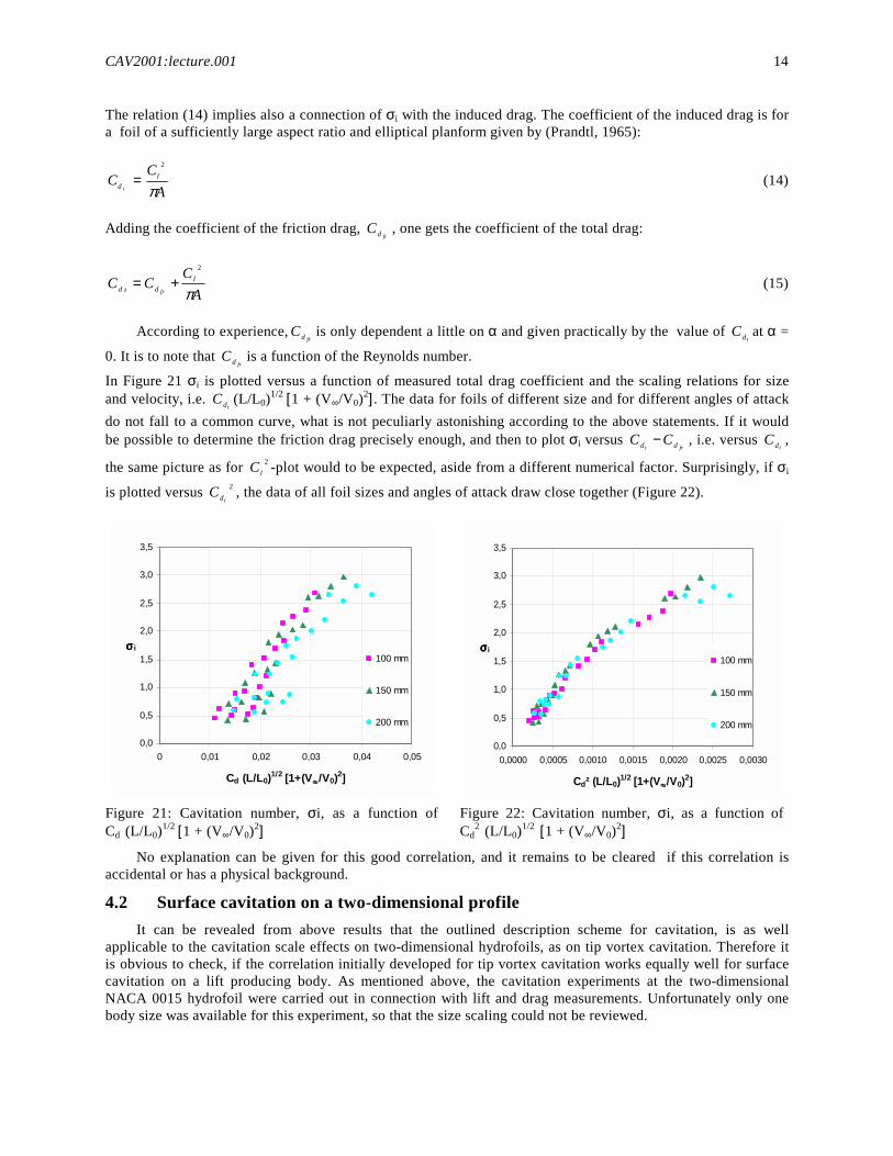
In Figure 21 σi is plotted versus a function of measured total drag coefficient and the scaling relations for size and velocity, i.e.

tdC (L/L0)1/2 [1 + (V∞/V0)2] . The data for foils of different size and for different angles of attack do not fall to a common curve, what is not peculiarly astonishing according to the above statements. If it would be possible to determine the friction drag precisely enough, and then to plot σi versus

frt dd CC − , i.e. versus idC ,

the same picture as for 2lC -plot would to be expected, aside from a different numerical factor. Surprisingly, if σi

is plotted versus 2

tdC , the data of all foil sizes and angles of attack draw close together (Figure 22).

0,0

0,5

1,0

1,5

2,0

2,5

3,0

3,5

0 0,01 0,02 0,03 0,04 0,05

Cd (L/L0)1/2 [1+(V����/V0)2]

σσσσ i100 mm

150 mm

200 mm

0,0

0,5

1,0

1,5

2,0

2,5

3,0

3,5

0,0000 0,0005 0,0010 0,0015 0,0020 0,0025 0,0030

Cd² (L/L0)1/2 [1+(V����/V0)2]

σσσσ i100 mm

150 mm

200 mm

Figure 21: Cavitation number, σi, as a function of Cd (L/L0)1/2 [1 + (V∞/V0)2]

Figure 22: Cavitation number, σi, as a function of Cd

2 (L/L0)1/2 [1 + (V∞/V0)2]

No explanation can be given for this good correlation, and it remains to be cleared if this correlation is accidental or has a physical background.

4.2 Surface cavitation on a two-dimensional profile It can be revealed from above results that the outlined description scheme for cavitation, is as well

applicable to the cavitation scale effects on two-dimensional hydrofoils, as on tip vortex cavitation. Therefore it is obvious to check, if the correlation initially developed for tip vortex cavitation works equally well for surface cavitation on a lift producing body. As mentioned above, the cavitation experiments at the two-dimensional NACA 0015 hydrofoil were carried out in connection with lift and drag measurements. Unfortunately only one body size was available for this experiment, so that the size scaling could not be reviewed.

CAV2001:lecture.001 15

0,0

1,0

2,0

3,0

4,0

5,0

6,0

100.000 1.000.000 10.000.000

Re

σσσσ i

3° 6°

9° 12°

0,0

1,0

2,0

3,0

4,0

5,0

6,0

0 50.000 100.000 150.000αααα 2 2 2 2 Re0,5

σσσσ i

3° 6°

9° 12°

Figure 23: Critical cavitation number, σI, versus Re-number for a two-dimensional NACA 0015 foil

Figure 24: Correlation of cavitation data of a NACA 0015 hydrofoil, using the classical McCormick relation, with exponents n = 2 and m = 0.5

In Figure 23 the σi-values are plotted versus the Re-number, and in Figure 24 the classical McCormick correlation with modified exponents n = 2 and m = 0.5 is applied to the test results. Comparable to the results for tip vortex cavitation (Figure 18) the data appear again well correlated, though the data points for one angle of attack form again curves, especially those for the smaller α. However, it is surprising and important at the same time that the correlation initially developed for tip vortex cavitation, works equally well for surface cavitation on a lift producing two-dimensional hydrofoil.

Using the Arndt type correlation, i.e. lift coefficient Cl instead of α shows a comparable quality of data correlation (here m= 0.4, following Arndt´s suggestion), but again the data sets for one angle of attack show an over-proportional increase of σi with Re-number, especially for small angles of attack (Figure 25).

0,0

1,0

2,0

3,0

4,0

5,0

6,0

0 100 200 300 400 500

CL2 Re0,4

σσσσ i

3° 6°

9° 12°

0,0

1,0

2,0

3,0

4,0

5,0

6,0

0 2 4 6 8

Cd Re0,4

σσσσ i

3° 6°

9° 12°

Figure 25: Correlation of cavitation data of a NACA 0015 hydrofoil, using the Arndt type relation

Figure 26: Correlation of cavitation data of a NACA 0015 hydrofoil, using the Arndt type relation with Cd instead of Cl

2

In the next three figures finally correlations using Cd are shown. In Figure 26 Cl2 is replaced by the linear

function of Cd, following the above argumentation about the relation of Cl and Cd. Again the data for different angles of attack do not fall to a common curve. But surprisingly again, if Cd

2 is used the data draw closer together (Figure 27). Finally using the empirical relation for velocity scaling [1 + (V∞/V0)2] instead of a power of Re in accordance with equ. (4) or (8), respectively, again brings about an improved correlation. The set of data points for all angles of attack fall now more or less onto a straight line aiming through zero.

CAV2001:lecture.001 16

0,0

1,0

2,0

3,0

4,0

5,0

6,0

0,00 0,05 0,10 0,15 0,20

Cd2 Re0,4

σσσσ i

3° 6°

9° 12°

y = 5271,5xR2 = 0,9926

0,0

1,0

2,0

3,0

4,0

5,0

6,0

0,0000 0,0002 0,0004 0,0006 0,0008 0,0010

Cd2 [1+(V

����/V0)2]

σσσσ i

3° 6°

9° 12°

Figure 27: The McCormick type correlation using Cd2 Figure 28: The correlation using Cd

2 and the empirical relation for velocity scaling (only one size)

The finding that the correlation, initially developed for tip vortex cavitation, works equally well for surface cavitation on a lift producing two-dimensional hydrofoil, is just as remarkable as the correlation obviously working best with the squared drag coefficient.

4.3 Surface and separated flow cavitation on non lift producing, arbitrarily shaped bodies

After all these findings it was only a natural extension to check if cavitation numbers for non lift producing, arbitrarily shaped bodies can be correlated with their drag coefficient, Cd, as well. Therefore non lift producing two-dimensional bodies were built and their drag forces measured with the existing force balance used for the two-dimensional NACA 0015 hydrofoil. A special force balance was constructed to measure the drag force of rotational symmetric bodies.

Investigated were two families of rotational symmetric bodies (blunt and hemispherical nosed bodies of 30 mm and 60mm) and in total 8 two-dimensional bodies with different noses and one example also of different size (see inserts in Figure 29 and Figure 30).

0,0

1,0

2,0

3,0

4,0

5,0

6,0

7,0

8,0

0 0,5 1 1,5 2Cd

2 (L/L0)1/2 [1+(V����/V0)2]

σσσσ i

rot. symm. blunt 30 mm rot. symm. blunt 60 mmrot. symm. hemisph. 30 mm rot. symm. hemisph. 60 mmtw o-dim. blunt 40 mm 0° tw o-dim. blunt 40 mm 15°tw o-dim. blunt 40 mm 30° tw o-dim. blunt 40 mm 45°tw o-dim. cal1/8 40 mm 0° tw o-dim. hemisph. 40 mm 0°tw o-dim. w edge 40 mm 0° tw o-dim. blunt 20 mm 0°

0,0

1,0

2,0

3,0

4,0

5,0

6,0

7,0

8,0

0 0,2 0,4 0,6 0,8

Cd (L/L0)1/2 [1+(V����/V0)2]

σσσσ i

rot. symm. blunt 30 mm rot. symm. blunt 60 mmrot. symm. hemisph. 30 mm rot. symm. hemisph. 60 mmtw o-dim. blunt 40 mm 0° tw o-dim. blunt 40 mm 15°tw o-dim. blunt 40 mm 30° tw o-dim. blunt 40 mm 45°tw o-dim. cal1/8 40 mm 0° tw o-dim. hemisph. 40 mm 0°tw o-dim. w edge 40 mm 0° tw o-dim. blunt 20 mm 0°

Figure 29: σi versus a function of Cd2 and the scaling

relations for size and velocity Figure 30: σi versus a linear function of Cd and the scaling relations for size and velocity

CAV2001:lecture.001 17

In order to make it short here in Figure 29 the results of all investigated non-lift producing bodies are plotted directly in the above found way of the best correlation for lift producing bodies, i.e. σi versus a function of Cd

2 and the scaling relations for size and velocity. Here quite obviously this correlation does not work satisfactorily. However, a linear plot of Cd indicates again a nearly perfect correlation of all the data (Figure 30).

5 Summary Experimental results of cavitation tests on all kinds of submerged bodies show a surprising uniformity in the

qualitative behavior, i.e. in the connection of cavitation number at cavitation inception and hydrodynamic parameters like e.g. size and flow velocity, independent of the type of the cavitation phenomenon. This lets presume a uniform mechanism for cavitation inception in spite of different forms of cavitation appearance. The obvious presumption is that in all the investigated cases it is the pressure reduction in vortices which leads to cavitation. In the case of vortex cavitation this mechanism is evident, but also in the cases of surface cavitation and cavitation in separated flows arguments for a uniform scheme of description can be put forward.

It can be stated that there exists a connection of pressure reduction in vortex cores, either in the induced vortex of lift producing bodies, or in the vortices of shear layers of turbulent and/or separated flow on arbitrary shaped bodies, respectively. and the drag which is caused by the continuous production of these vortices.

In the case of tip vortex cavitation there exists an interpretation scheme following McCormick, σi ≈ αn Rem. The first factor of the right side of the equation is explained by the circulation of the induced vortex which defines the lift, and which is via the lift connected with α. The second factor considers the structure of the vortex core, which is dependent on the boundary layer at the hydrofoil and thus on the Re-number. The proportionality of the cavitation number to α2 means at the same time proportionality to the coefficient of induced drag as equ. (12) and (14) imply.

The astonishingly good correlation of σi and squared total drag, Cd2, in the case of tip vortex cavitation and

surface cavitation of a lift producing foil is in contradiction of equ. (14) and (15), which are fundamental in hydrofoil theory. If it would be possible to discern precisely enough between the friction drag and the induced drag or shape drag, respectively, the theoretically expected correlation could eventually be seen.

The good correlation of σi and measured drag on non-lift producing bodies bridges the two empirically found basic correlations. The vortex system in such boundary layers form the shape drag, which is in most cases much bigger than the pure friction drag developing in unseparated flow. Hence, in this case σi should be predominantly proportional to the measured total drag, and explain the empirically found proportionality to the measured coefficient of the total drag, Cd.

Concerning the over proportional increase of σi with flow velocity, no plausible explanation can be made until now, even not with the vortex model. Turbulent flow fluctuations are kinetically connected with mean flow, and thus scale with V∞. Turbulent pressure fluctuations accordingly scale with ρV∞

2. The experimentally found additional factor V∞

2 is still to be explained. However, the new findings about the correlation of cavitation numbers with drag coefficients are believed to be the clue to why the empirically found scaling relations are so universal, and a key to the physical explanation for these scale effects.

Nomenclature A aspect ratio = 8b/πco b (m) half span c0 (m) maximum chord length Cl lift coefficient Cd drag coefficient Cp pressure coefficient, (P-P∞)/(0.5 ρ V∞

2) Cpmin minimum pressure coefficient k, K, K1, K2 constants, characteristic shape factor K0 basic value of K for turbulence level 0 % L; L0 (m) characteristic and reference length (i.g. 1 m) m, n exponents P∞ (N/m2) reference pressure Pts (N/m2) water tensile strength

CAV2001:lecture.001 18

Pv (N/m2) vapor pressure Re Reynolds number S, S0 (m/s) standard and reference standard deviation of the free stream velocity Tu turbulence level V∞ (m/s) free stream velocity V0 (m/s) reference velocity, V0 ≅ 12 m/s fits results best σ cavitation number, (P∞ - Pv) / (0.5 ρ V∞

2) σ´ modified. cavitation number σi cavitation inception number σd desinent cavitation number σ0 basic cavitation number for V∞ = 0 α angle of attack α0 angle of attack of zero lift ν (m2/s) cinematic viscosity of fluid ν0 (m2/s) reference viscosity at 20°C

References Ackeret, J.: "Experimentelle und theoretische Untersuchungen über Hohlraumbildung (Kavitation) im Wasser",

Technische Mechanik und Thermodynamik, Monatliche Beihefte zur VDI-Zeitschrift, Berlin, Bd. 1, Nr. 1 und 2,1930

Arndt, R.E.A., Dugue Ch..: "Recent Advances in Tip Vortex Cavitation Research", Proceedings International Symposium on Propulsors and Cavitation, Hamburg, Germany, 1992

McCormick Jr., B.W.: “On Cavitation Produced by a Vortex Trailing From a Lifting Surfaces”, Journal of Basic Engineering, September 1962

Eickmann G. :"Maßstabsgesetze der beginnenden Kavitation", Dissertation, Munich University of Technology, Rep. No.69 of the Hydraulic Laboratory Obernach, 1992

Hamitt, F. G.: "Cavitation an Multiphase Flow Phenomena", McGraw-Hill Int. Book Comp. 1980 Holl, J.W., Billet, M.L., Kobi, D., Meyer, R.S., Dreyer, J.J.: “Effect of Microbubble Seeding on Cavitation

Inception”, Cavitation and Multiphase Flow Forum, ASME FED Vol. 50, 1987 ITTC: Report of the Cavitation Committee, Appendix A, 1978 Keller, A.P.: "Tensile Strength of Liquids", Proc. of the 5th Intern. Symp. on Water Column Separation, IAHR

Work Group, Obernach 1981 Keller, A.P.: "Maßstabseffekte bei der Anfangskavitation unter Berücksichtigung der Zugspannungsfestigkeit der

Flüssigkeit", Pumpentagung Karlsruhe, 1984 Keller A.P., Eickmann G.: “Velocity and Size Scale Effects for Incipient Cavitation of Axisymmetric Bodies in

Water of Different Quality”, International Symposium on Cavitation Inception, American Society of Mechanical Engineers (ASME), San Francisco, pp. 79-86, December 1989

Keller, A.P., Kuzman-Anton, A.F.: "Scaling of cavitation inception in liquids of higher viscosity than water, under consideration of the tensile strength of the liquids", 2eme Journees Cavitation, Societe Hydrotechniques de France, Paris, 1992

Keller, A.P.: "New Scaling Laws for Hydrodynamic Cavitation Inception", The Second International Symposium on Cavitation, Tokyo, Japan, 1994

Keller, A.P.: "The Effect of Flow Turbulence on Cavitation Inception", ASME Fluids Engineering Division Summer Meeting, Vancouver, June 1997

Kuhn de Chizelle, Y., Brennen, C:E., Ceccio, S.L., Gowing, S.: "Scaling Experiments on the Dynamics and Acoustics of Traveling Bubble Cavitation", International Conference on Cavitation, Proceedings of the Institution of Mechanical Engineer, Cambridge, 1992

Prandtl L.: “Führer durch die Strömungslehre”, Vieweg Braunschweig, 1965