Congressional Budget Office

Modeling for Public Policy Analysis: Emerging Trends and Future DirectionsThe Australian Treasury

Sydney, Australia

February 23, 2017

Wendy EdelbergAssociate Director for Economic Analysis

CBO’s Assessment of the Long-Term Budget Outlook and Its Approach to Dynamic Analysis

1CO N G R ES S I O N A L B U D G E T O F F I C E

Overview

■ Summary of CBO’s long-term budget projections

■ CBO’s approach to dynamic analysis

■ An example: an illustrative dynamic analysis of changes in spending on federal investment

2CO N G R ES S I O N A L B U D G E T O F F I C E

The Long-Term Budget Outlook

3CO N G R ES S I O N A L B U D G E T O F F I C E

If current laws governing taxes and spending did not change, the condition of the federal budget would worsen considerably over the next three decades, as debt grew larger in relation to the economy than ever recorded in U.S. history.

4CO N G R ES S I O N A L B U D G E T O F F I C E

Federal Debt, Spending, and Revenues

5CO N G R ES S I O N A L B U D G E T O F F I C E

The Federal Budget Under the Extended Baseline

6CO N G R ES S I O N A L B U D G E T O F F I C E

Because of the growing federal deficits, federal debt held by the public is projected to total 145 percent of GDP in 2047.

The prospect of such large debt poses substantial risks for the United States and presents U.S. policymakers with significant challenges.

7CO N G R ES S I O N A L B U D G E T O F F I C E

Federal Debt Held by the Public, 1790 to 2047Percentage of GDP

8CO N G R ES S I O N A L B U D G E T O F F I C E

CBO’s Approach to Dynamic Analysis

9CO N G R ES S I O N A L B U D G E T O F F I C E

CBO has routinely produced dynamic analysis of fiscal policies.

■ Analysis of the President’s Budget

■ Long-term budget and economic outlooks

■ Analyses of illustrative fiscal policy scenarios

10CO N G R ES S I O N A L B U D G E T O F F I C E

Behavioral responses to proposed policies are incorporated in CBO’s conventional estimates.

But, CBO’s conventional cost estimates generally do not reflect changes in behavior that would affect overall output, such as any changes in labor supply or private investment resulting from changes in fiscal policy.

11CO N G R ES S I O N A L B U D G E T O F F I C E

The 2016 Budget Resolution set out a requirement for CBO and the Joint Committee on Taxation to incorporate the budgetary impact of macroeconomic effects into its 10-year cost estimates for “major” legislation that Congressional authorizing committees approve.

12CO N G R ES S I O N A L B U D G E T O F F I C E

Changes in fiscal policies affect the overall economy in the short term primarily by influencing the demand for goods and services, which leads to changes in output relative to potential (maximum sustainable) output.

13CO N G R ES S I O N A L B U D G E T O F F I C E

Changes in fiscal policies affect the economy in the long term by influencing potential output through changes in

■ national saving,

■ foreign investment in the United States,

■ federal investment, and

■ people’s incentives to work and save, as well as businesses’ incentives to invest.

14CO N G R ES S I O N A L B U D G E T O F F I C E

■ CBO uses two models of potential output to estimate the effects of changes in fiscal policies on the overall economy over the long term.– Solow-type growth model– Life-cycle growth model

■ Potential output depends on two major factors.– Amount and quality of labor and capital (which depend on work,

public and private saving, and investment)– Productivity of the labor and capital inputs (which depends in part on

federal investment)

15CO N G R ES S I O N A L B U D G E T O F F I C E

■ CBO estimates the macroeconomic feedback to the budget through a simplified analysis that accounts for changes in taxable income, interest rates, and prices, among other things.

■ The agency does not perform a detailed, program-by-program analysis of the effects on the budget, as it does in other contexts.

16CO N G R ES S I O N A L B U D G E T O F F I C E

Reporting Uncertainty in Estimates Related to Dynamic Analysis

17CO N G R ES S I O N A L B U D G E T O F F I C E

Central Estimates and Ranges

■ CBO’s estimates of effects are based on parameters such as the extent to which national saving is altered by changes in fiscal policies.

■ Parameter values are uncertain. In most cases, CBO estimates economic effects (and feedback to the budget) using a range of parameter estimates reflecting the consensus in the economic literature.

■ To arrive at its central estimate of the economic effects, CBO uses the central estimates for those parameters.

18CO N G R ES S I O N A L B U D G E T O F F I C E

Uncertainty in Outcomes

■ When practicable and informative, CBO reports the estimated range of outcomes owing to the uncertainty of macroeconomic effects.

■ CBO reports a range of estimates using only results from the Solow-type growth model.

– Differences between those results and estimates from the life-cycle model reflect model uncertainty in addition to parameter uncertainty.

– Such differences make interpretation difficult.

■ When the uncertainty of the direct budgetary effects of the policy is substantial, that range for the macroeconomic feedback would not be a useful indicator of the uncertainty of the overall estimate.

19CO N G R ES S I O N A L B U D G E T O F F I C E

Uncertainty in Outcomes (Continued)

■ The likelihood that all parameters would simultaneously be at the ends of their ranges is smaller than the likelihood that any single parameter would be at the end of its range. – CBO has focused on uncertainty about the two parameters that have the

largest budgetary effects.– CBO has reported estimates resulting from cases in which two

parameters are at the ends of their ranges and other parameters are equal to their central estimates.

■ CBO reports cases that show the most favorable and least favorable budgetary outcomes.

20CO N G R ES S I O N A L B U D G E T O F F I C E

Analyzing Short-Term Economic Effects

21CO N G R ES S I O N A L B U D G E T O F F I C E

Short-Term Effects From Changes in Demand

■ Changes in purchases by federal agencies and by people who receive federal payments and pay taxes contribute directly to overall demand.

■ The change in output for each dollar of direct contribution to demand (the “demand multiplier”) varies with the response of monetary policy.

22CO N G R ES S I O N A L B U D G E T O F F I C E

Short-Term Effects From Changes in Demand: CBO’s Estimates of the Demand Multiplier

■ When the monetary policy response is likely to be limited, the demand multiplier over four quarters ranges from 0.5 to 2.5, with a central estimate of 1.5.

■ When the monetary policy response is likely to be stronger, the demand multiplier over four quarters ranges from 0.4 to 1.9, with a central estimate of 1.2; over eight quarters, it ranges from 0.2 to 0.8, with a central estimate of 0.5.

23CO N G R ES S I O N A L B U D G E T O F F I C E

Short-Term Effects From Changes in the Supply of Labor

■ Effects on the supply of labor can lead to changes in employment in the short term.

■ The extent of the change in employment depends on the amount of slack in the labor market.

24CO N G R ES S I O N A L B U D G E T O F F I C E

Analyzing Long-Term Economic Effects

25CO N G R ES S I O N A L B U D G E T O F F I C E

Estimated Effects on the Overall Economy

■ Generally, CBO focuses on effects on gross national product (GNP) instead of the more commonly cited gross domestic product (GDP).

■ GNP is the total market value of goods and services produced in a given period by the labor and capital supplied by a country’s residents, regardless of where the labor and capital are located.

■ GNP excludes foreigners’ earnings on domestic investments and includes domestic residents’ foreign earnings.

■ In a large, open economy like that of the United States, changes in GNP are a better measure of changes in domestic residents’ income than are changes in GDP.

26CO N G R ES S I O N A L B U D G E T O F F I C E

The Role of Expectations About Fiscal Policy: Solow-Type Growth Model

■ People base their decisions about working and saving primarily on current economic conditions, including government policies.

■ Decisions reflect people’s anticipation of future policies in a general way but not their responses to specific future developments.

27CO N G R ES S I O N A L B U D G E T O F F I C E

The Role of Expectations About Fiscal Policy: Life-Cycle Growth Model

■ Households in the life-cycle model make choices about working and saving in response to both current economic conditions and their explicit expectations of future economic conditions.

■ The model requires specification of future fiscal policies that put federal debt on a sustainable path over the long run.

■ If debt as a percentage of GDP were to rise without limit, households in the model would anticipate that eventually there would not be sufficient resources to finance the debt.

28CO N G R ES S I O N A L B U D G E T O F F I C E

How the Supply of Labor Responds to Changes in Fiscal Policy in the Solow-Type Growth Model

■ The overall effects of a policy change on the labor supply can be expressed as an elasticity, which is the percentage change in the labor supply resulting from a 1 percent change in after-tax income. – Substitution effect: Increased after-tax compensation for an additional

hour of work makes work more valuable relative to other uses of a person’s time.

– Income effect: Increased after-tax income from a given amount of work allows people to maintain the same standard of living while working fewer hours.

29CO N G R ES S I O N A L B U D G E T O F F I C E

How Labor Supply Responds to Changes in Fiscal Policy in the Solow-Type Growth Model (Continued)

■ CBO’s central estimate corresponds to an earnings-weighted total wage elasticity for all earners of 0.19 (composed of a substitution elasticity of 0.24 and an income elasticity of –0.05).

■ For some proposals, income and substitution effects may not offset each other (for example, if the proposal would increase after-tax wages but reduce income).

■ CBO estimates that the substitution elasticity could range from about 0.16 to about 0.32; the income elasticity could range from about –0.10 to about 0.

30CO N G R ES S I O N A L B U D G E T O F F I C E

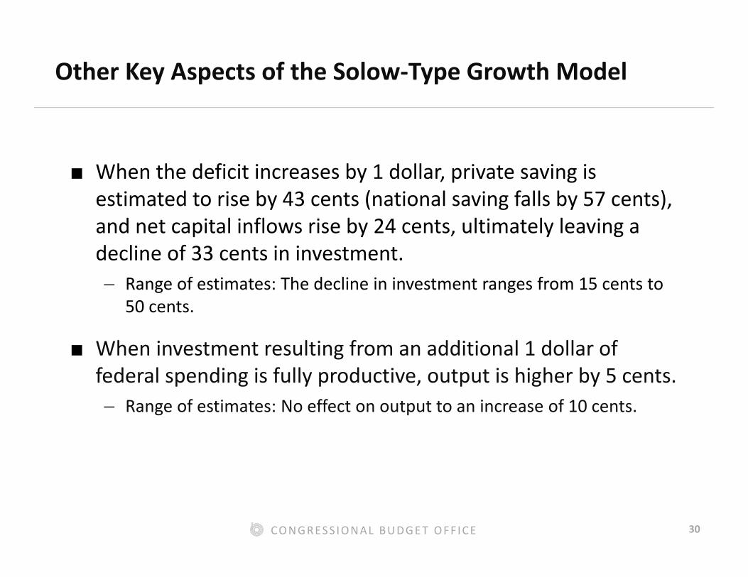
Other Key Aspects of the Solow-Type Growth Model

■ When the deficit increases by 1 dollar, private saving is estimated to rise by 43 cents (national saving falls by 57 cents), and net capital inflows rise by 24 cents, ultimately leaving a decline of 33 cents in investment.– Range of estimates: The decline in investment ranges from 15 cents to

50 cents.

■ When investment resulting from an additional 1 dollar of federal spending is fully productive, output is higher by 5 cents.– Range of estimates: No effect on output to an increase of 10 cents.

31CO N G R ES S I O N A L B U D G E T O F F I C E

Key Aspects of the Life-Cycle Growth Model

■ The model includes different cohorts of households, also known as “overlapping generations.”

■ The model requires explicitly specifying people’s expectations regarding how fiscal policy and the economy will evolve.

■ People are assumed to know, with certainty, the paths of overall outcomes, such as after-tax rates of return.

■ Paths of a particular household’s after-tax wages (and thus its Social Security benefits) are uncertain.

32CO N G R ES S I O N A L B U D G E T O F F I C E

Risk in the Life-Cycle Growth Model

■ People face idiosyncratic risk related to their own future income.

■ People do not know how long they will live.

■ Because of that risk, households in the life-cycle growth model take the precaution of holding additional savings as a buffer against potential drops in income or the need for resources in retirement over the course of an unusually long life.

33CO N G R ES S I O N A L B U D G E T O F F I C E

Other Key Aspects of the Life-Cycle Growth Model

■ Labor supply and private saving are influenced by the current values and future anticipated values of the after-tax rate of return on saving, the after-tax wage, and households’ disposable income, among other factors.

■ The elasticity with respect to a one-time temporary change in wages (the so-called Frisch elasticity) is 0.40, according to CBO’s central estimates, with a range from 0.27 to 0.53.– Frisch elasticity and CBO’s estimate of the total wage elasticity are

chosen to be consistent with each other.

34CO N G R ES S I O N A L B U D G E T O F F I C E

Other Key Aspects of the Life-Cycle Growth Model (Continued)

■ People decide how much to work and save to make themselves as well off as possible over their lifetime but do not consider the well-being of their children.

■ Without altruism, a household’s responsiveness to a policy change depends on the ages of the people in the household.

■ Older generations are constrained in how they can adjust to policy changes.

■ If the people forming a household die with wealth, in the model that wealth is uniformly distributed to working-age households. The size of that overall transfer is predictable.

35CO N G R ES S I O N A L B U D G E T O F F I C E

Range of Estimates Within the Life-Cycle Growth Model

To consider a broad range of possibilities about net capital inflows, CBO analyzes the effects of fiscal policy changes under two alternative assumptions:

■ First, net capital inflows are unaffected by changes in fiscal policies (equivalently, that the country has, in effect, a so-called closed economy).

■ Second, net capital inflows change by the full amount necessary to offset any effect of changes in fiscal policies on interest rates (equivalently, that the country has, in effect, a so-called small, open economy).

36CO N G R ES S I O N A L B U D G E T O F F I C E

Range of Estimates Within the Life-Cycle Growth Model (Continued)

■ Because the model is forward-looking, it requires offsetting policy changes that eventually stabilize government debt (closure rules); beginning in 15 years, those policies would be phased in over 10 years.

■ CBO models two sets of assumptions:– Reduced spending (half from government purchases and half from

transfers)– Increased taxes (half from marginal rate changes and half in lump-sum

amounts)

■ CBO reports both closure rules, and results generally are similar.

37CO N G R ES S I O N A L B U D G E T O F F I C E

An Example: Illustrative Changes in Spending on Federal Investment Financed by Federal Borrowing

38CO N G R ES S I O N A L B U D G E T O F F I C E

Federal investment affects the economy mainly by changing overall demand in the short term and private-sector productivityin the longer term.

39CO N G R ES S I O N A L B U D G E T O F F I C E

CBO’s Interpretation of the Empirical Literature on Long-Term Economic Effects of Federal Investment

40CO N G R ES S I O N A L B U D G E T O F F I C E

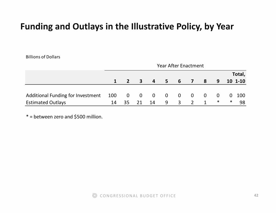
Consider an illustrative policy that CBO analyzed in June 2016: a one-time $100 billion boost in funding for federal investment financed by federal borrowing.

41CO N G R ES S I O N A L B U D G E T O F F I C E

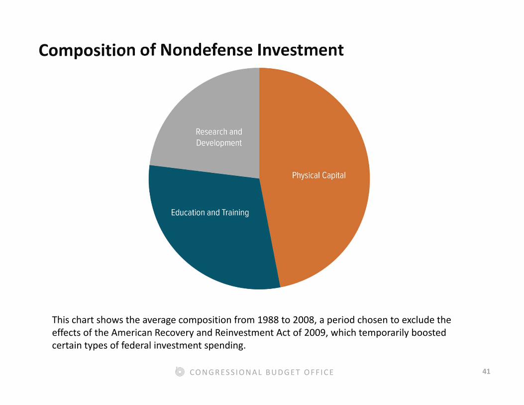
Composition of Nondefense Investment

This chart shows the average composition from 1988 to 2008, a period chosen to exclude the effects of the American Recovery and Reinvestment Act of 2009, which temporarily boosted certain types of federal investment spending.

42CO N G R ES S I O N A L B U D G E T O F F I C E

Funding and Outlays in the Illustrative Policy, by Year

Billions of Dollars

Year After EnactmentTotal,

1 2 3 4 5 6 7 8 9 10 1-10

Additional Funding for Investment 100 0 0 0 0 0 0 0 0 0 100Estimated Outlays 14 35 21 14 9 3 2 1 * * 98

* = between zero and $500 million.

43CO N G R ES S I O N A L B U D G E T O F F I C E

The Share of Federal Investment That Becomes Productive Under the Illustrative Policy

44CO N G R ES S I O N A L B U D G E T O F F I C E

How much a boost in federal investment increases the size of the public capital stock, on net, depends primarily on two factors:

The response of state and local governmentsAcknowledging great uncertainty, CBO estimates that one-third of the change in the typical dollar of federal investment is offset by changes in investment by state and local governments.

How quickly that capital depreciatesThe typical dollar of federal investment depreciates at an annual rate of 2 percent, CBO estimates.

45CO N G R ES S I O N A L B U D G E T O F F I C E

Limitations and Uncertainty of Analysis of Federal Investment

46CO N G R ES S I O N A L B U D G E T O F F I C E

Estimates for typical investment should not be used to directly infer the effects of particular investment proposals. ■ Some investments start improving productivity

soon after they are made, whereas others take much longer.

■ Similarly, some investments have stronger effects on productivity than others do.

■ The way that states, local governments, and private entities adjust their own investment spending and borrowing in response to changes in federal investment can also vary, depending on the proposal.

47CO N G R ES S I O N A L B U D G E T O F F I C E

When possible, CBO’s analyses of proposals reflect estimated effects on timing, productivity, and responses of other investors that are specific to the types of investment being considered.■ In many cases, however, empirical evidence is

scant–particularly on productivity effects of some kinds of investment and the responses of other investors.

■ In such cases, CBO uses the estimated effect of typical federal investment.

48CO N G R ES S I O N A L B U D G E T O F F I C E

CBO’s Likely Range of the Effect on Output From an Increase in the Typical Kind of Federal Investment

In CBO’s assessment, there is roughly a two-thirds chance that the effect on GDP would be in a “likely range” between zero and 10 cents.

49CO N G R ES S I O N A L B U D G E T O F F I C E

The Effect on Output and the Deficit of the Illustrative Policy Financed by Borrowing

50CO N G R ES S I O N A L B U D G E T O F F I C E

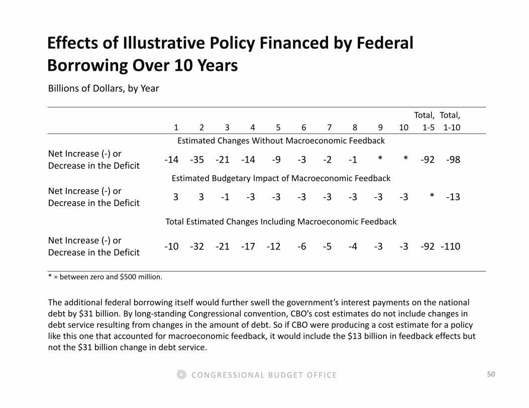
Effects of Illustrative Policy Financed by Federal Borrowing Over 10 YearsBillions of Dollars, by Year

Total, Total,1 2 3 4 5 6 7 8 9 10 1-5 1-10Estimated Changes Without Macroeconomic Feedback

Net Increase (-) or Decrease in the Deficit -14 -35 -21 -14 -9 -3 -2 -1 * * -92 -98

Estimated Budgetary Impact of Macroeconomic FeedbackNet Increase (-) or Decrease in the Deficit 3 3 -1 -3 -3 -3 -3 -3 -3 -3 * -13

Total Estimated Changes Including Macroeconomic Feedback

Net Increase (-) or Decrease in the Deficit -10 -32 -21 -17 -12 -6 -5 -4 -3 -3 -92 -110

* = between zero and $500 million.

The additional federal borrowing itself would further swell the government’s interest payments on the national debt by $31 billion. By long-standing Congressional convention, CBO’s cost estimates do not include changes in debt service resulting from changes in the amount of debt. So if CBO were producing a cost estimate for a policy like this one that accounted for macroeconomic feedback, it would include the $13 billion in feedback effects but not the $31 billion change in debt service.

51CO N G R ES S I O N A L B U D G E T O F F I C E

Billions of DollarsChange in Gross Domestic Product

Central Estimate 45Likely Range -32 to 129

Increase (-) in the Deficit From Macroeconomic Feedback on the Budget

Central Estimate -13Likely Range -5 to -22

Total Increase (-) in the Deficit, Including Direct Effects

Central Estimate -110Likely Range -102 to -119

Cumulative Effects of Illustrative Policy Financed by Federal Borrowing Over 10 Years

52CO N G R ES S I O N A L B U D G E T O F F I C E

Notes

For more information about CBO’s most recent budget projections, as well as the agency’s approach to dynamic analysis and, more specifically, to analyzing changes in federal investment, see the following:

■ The Budget and Economic Outlook: 2017 to 2027(January 2017), www.cbo.gov/publication/52370.

■ Congressional Budget Office, “Economic Effects of Fiscal Policy,” www.cbo.gov/topics/economy/economic-effects-fiscal-policy.

■ The Macroeconomic and Budgetary Effects of Federal Investment (June 2016), www.cbo.gov/publication/51628.