8/11/2019 CCB12C3Cd01

http://slidepdf.com/reader/full/ccb12c3cd01 1/4

 Abstract --An assumption of complete spatial randomness has

been used to obtain analytic expressions that describe the

probability that the closest   lightning strike is within any

distance of an arbitrary point or a simulated power line, if the

area density of strikes in the region is known. Preliminary

tests of these functions show that they describe experimental

data rather well, but such tests are limited by the accuracy of 

the measurements.

I. I NTRODUCTION

ATED, wideband lightning sensors [1] similar to those

used in the U.S. National Lightning Detection Network 

(NLDN) [2,3] have been used in many countries for many

years, and the resulting data provide accurate estimates of the

area-density of cloud-to-ground (CG) lightning flashes under 

individual storms and over larger regions on monthly,

seasonal, and annual time scales (see, for example, [4] and the

references therein). Here, we will show how knowledge of the

average area density of strikes,  N  g , in a region can be used to

estimate the chances that a strike has occurred within any

given distance of a random point or line segment in that region.

II. NEAREST -STRIKE TO A POINT

We begin by supposing that we know the average area-

density of strikes,  N  g , and we want to know the chances that

any strike has occurred within a distance,  R, of any origin

(chosen at random) in that region. We assume that each strike

is a random event and that the spatial pattern of the strike

 points has a homogeneous Poisson distribution, i.e.,  N  g   has

complete spatial randomness. With this assumption, we can

use the method outlined in [5, 6] to derive the probability

density, w(r) , for the nearest  strike being within a distance r 

and r + dr  of the origin, i.e.

+=

dr r andr between

strikeaIS y thereProbabilit

r withinisstrike

  NOy thatProbabilit )( dr r w

or 

 This work was supported in part by the NASA Kennedy Space

Center, Grant NAG10-302.

E. Philip Krider is with the Institute of Atmospheric Physics,

University of Arizona, Tucson, AZ 85721 USA. (e-mail:

krider@atmo.arizona.edu)

( )   ( ) 10

 when2r 

0 )dr'w(r'1   =∫ 

∞∫ −=    

  

  

dr' r' w g  prdr N w(r)dr .

Solving this equation, we obtain the nearest-neighbor 

distribution,

     

  −= 2

g Nexpg N2)( r rdr dr r w   ππ . (1)

Using (1), it is straightforward to show that the most probable

nearest-neighbor distance is

g2

1

 N r  pro bab lemost 

π

= , the mean is

 g  N r 

2

1= , and the variance is

( ) .0683.0

44

 g  N  g  N r Var    =−=

π

π

The integral of (1) describes the probability that the closest

strike is within a distance R,

')'()(

0

∫ =≤ R

dr r w R P  ,

or 

  )2g Nexp(1)(  R R P    π−−=≤ . (2)

 Now, if P is specified, (2) can be solved for R,

  [ ] 2/1)1ln(  g  N  P  R   π−−= . (3)

It should be noted that in cases where 12 << R N  g π ,

equation (2) reduces to

2)(  R N  R P   g π≈≤ .

III. NEAREST -STRIKE TO A LONG LINE SEGMENT

One can use the same ideas to derive the probability that

the closest (random) strike is between horizontal distance, h,

and h + dh (on either side) of a long line of length, L,

 Lh) N (  Ldh N  p(h)dh  g  g  2exp2   −= . (4)

On the Chances of Being Struck 

 by Cloud-to-Ground LightningE. Philip Krider , Member, IEEE 

G

0-7803-7967-5/03/$17.00 ©2003 IEEE

Paper accepted for presentation at 2003 IEEE Bologna Power Tech Conference, June 23th-26th, Bologna, Italy

8/11/2019 CCB12C3Cd01

http://slidepdf.com/reader/full/ccb12c3cd01 2/4

With (4), the most probable h is zero, the mean is

 g  LN h

2

1= , and the variance is ( )

( )22

1

 g  LN 

hVar    = .

An integral of (4) gives the probability that the closest strike is

within a distance H  of the line,

  ( )  LH) N (  H  P   g 2exp1   −−=≤ , (5)

and if P  and L are specified, then

   g  LN  P  H  2)1ln(   −−= . (6)

In cases where 12   << LH  N  g  , then (5) becomes

 LH  N  H  P   g 2)(   ≈≤ .

IV. COMPARISON WITH LIGHTNING DAT A

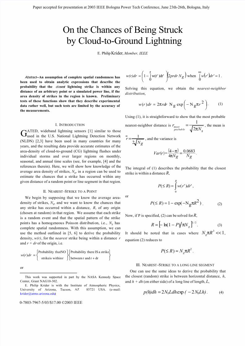
Figure 1 shows the spatial pattern of 7205 CG lightning

flashes that were recorded by the NLDN near Denver, Colo-

rado, over a 5-year period. Here, each dot shows the most

 probable location of the first return stroke in each flash (see

the Appendix in [2]), and in the following we will refer to these

 points as events. (Note: we have made no corrections for an

imperfect NLDN detection efficiency or for the multiple

attachment points that commonly occur in CG flashes [7].)

 

Fig. 1. Plot of CG lightning flash locations near Denver, CO from

January, 1995, through December, 1999. There are a total of 4786

strikes in the analysis sub-region shown by the dashed red line.

The data in Figure 1 have a numerical precision of four decimal

digits in latitude and longitude, which translates to a spatial

resolution of about 10 m, but random and systematic errors in

the NLDN typically produce location errors that are of the

order 0.5 to 1 km [2,3]. There were 4786 events within the 16x16

km2 analysis sub-region (to avoid edge effects) that is outlined

 by the dashed line in Figure 1, and the average value of  N  g 

over that region is 18.7 flashes per km2.

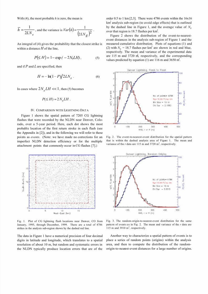
Figure 2 shows the distribution of the event-to-nearest-

event distances in the analysis sub-region of Figure 1 and the

measured cumulative distribution. Plots of equations (1) and

(2) with N  g   = 18.7 flashes per km2  are shown in red and blue,

respectively. The mean and variance of the experimental dataare 115 m and 3720 m

2, respectively, and the corresponding

values predicted by equation (1) are 116 m and 3650 m2.

Fig. 2. The event-to-nearest-event distribution for the spatial pattern

that is within the dashed analysis area of Figure 1. The mean and

variance of the r  data are 115 m and 3720 m2, respectively.

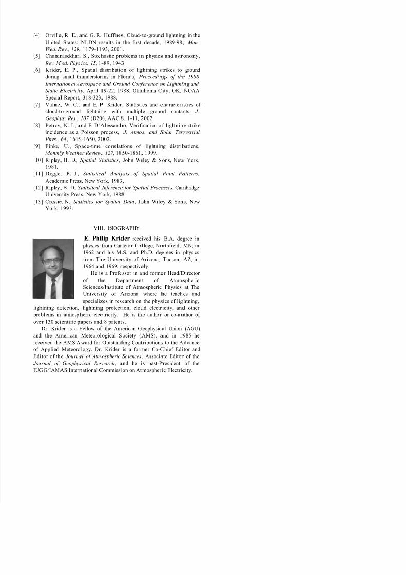
Fig. 3. The random-origin-to-nearest-event distribution for the same

 patte rn of events as in Fig. 2. The mean and variance of the r  data are

115 m and 3910 m2, respectively.

Another way to characterize a spatial pattern of events is to

 place a series of random points (origins) within the analysis

area, and then to compute the distribution of the random-

origin-to-nearest-event distances for a large number of origins.

8/11/2019 CCB12C3Cd01

http://slidepdf.com/reader/full/ccb12c3cd01 3/4

(Note: if the spatial distribution of events is truly uniform and

completely random, this distribution should be the same as the

event-to-nearest-event distribution that is shown in Figure 2.)

Figure 3 shows the random-origin-to-nearest-event distribution

that was computed for the same pattern of events as Figure 2,

using the same number of random origins as there are events in

Figure 2. The mean and variance of the nearest distances are

115 m and 3910 m2, respectively, and are very close to the

values that were obtained in Figure 2 (and predicted by

equation (1)).

Figure 4 shows the distribution of nearest-event distances

that was computed by placing 4786 random line segments,

each with a length of 1.0 km, at random locations and with

random orientations into the same pattern of events that was

used to compute Figure 3. The red and blue curves show

equations (4) and (5), respectively, with  L = 1.0 km and  N  g   =

18.7 flashes per km2. The sample mean and variance were 28.5

m and 853 m2, respectively, and it should be noted that each of 

these values is in good agreement with the predictions of 

equation (4), namely 26.7 m and 715 m2, respectively.

Fig. 4. Simulated line-to-nearest-event distribution for 4786 random (1.0

km) line segments placed within the same pattern of events that was

used in Figures 2 and 3. The mean and variance of the closest st rike

distances, h, are 28.5 m and 853 m2, respectively.

V. DISCUSSION

Figures 2–4 show that equations (1, 2, 4, 5) do describe the

measured, long-term patterns of the nearest-strike distancesrather well, but of course, such tests are limited by the

accuracy of the NLDN measurements on small spatial scales.

The most probable distances are in good agreement with

equations (1) and (4), and the values of the reduced chi-square,

a “goodness of fit” parameter, are excellent. The sample means

and variances are also in good agreement with model

 predictions; in fact, they are well within the 0.5 to 1.0 km

location accuracy of the NLDN.

As examples of possible applications of the above, let us

consider a region that has an average area density of 6.0 CG

strikes per km2, a representative value for the annual   area

density over much of the U.S. From equations (1) and (3), we

can say that, in such a region, the most probable nearest-strike

distance from any point (or person) will be 163 m, and there is a

50-50 chance of a strike within 192 m and a 10% chance of a

strike within 75 m. From equations (4) and (6), we can also say

that in this region, the average nearest-strike distance from

each 1.0 km line segment is 83 m, each segment has a 50-50

chance of a strike within 57 m, and there is a 10% chance of a

strike within 9 m of each segment.

Of course, the above estimates are really only valid over 

spatial scales that range from a few tens of meters on the low

end to tens of kilometers on the upper end. At smaller 

distances, the primary factors controlling the strike probability

(in addition to the presence of a lightning leader) are the

number and lengths of the upward connecting leaders, and

these factors depend on the size and geometry of the strike

object [8], the presence and size of any other objects in the

local vicinity of the strike object, and the strength of the

electric field under the downward-propagating leader. At

larger distances, N  g  may not be spatially uniform [9].

If the measurements of  N  g   show clusters of strike points,

such as might occur if there has been an unusually active

storm in the region, then the event-to-nearest-event

distributions (like Figure 2) will contain more events at short

distances than our model predicts, and if  N  g  contains holes or 

regions of reduced area density, then the nearest-neighbor 

distributions will contain more large distances. In any case,

even if  N  g   is not completely uniform, the assumption of 

complete spatial randomness can still be used as the null

hypothesis when applying various statistical tests to identify

and quantify the underlying spatial pattern and to find the

optimum value of N  g  (see, for example, [10-13]).

VI. ACKNOWLEDGMENTS

The author greatly appreciates the assistance of Kenneth E.

Kehoe in computing the nearest neighbor distributions and in

 programming the Monte Carlo simulations. The NLDN data

were provided by Vaisala-GAI, Tucson, AZ. This research has

 been supported in part by the NASA Kennedy Space Center 

under Grant NAG10-302.

VII. R EFERENCES

[1] Krider, E. P., R. C. Noggle, and M. A. Uman, A gated, wide-band

lightning direction finder for lightning return strokes,  J. Appl. Met.,

15 , 301-306, 1976.

[2] Cummins, K. L., M. J. Murphy, E. A. Bardo, W. L. Hiscox, R. B.

Pyle,, and A. E. Pifer, A combined TOA/MDF technology upgrade

of the U.S. National Lightning Detection Network,  J. Geophys.

 Res., 103 (D8), 9035-9044, 1998a.

[3] Cummins, K. L., E. P. Krider, and M. D. Malone, The U. S.

 National Lightning Detection Network and applications of cloud-

to-ground lightning data by electric power utilities,  IEEE Trans. on

 EMC, 40(4), 465-480, November, 1998b.

8/11/2019 CCB12C3Cd01

http://slidepdf.com/reader/full/ccb12c3cd01 4/4

 

[4] Orville, R. E., and G. R. Huffines, Cloud-to-ground lightning in the

United States: NLDN results in the first decade, 1989-98,  Mon.

Wea. Rev., 129, 1179-1193, 2001.

[5] Chandrasekhar, S., Stochastic problems in physics and astronomy,

 Rev. Mod. Physics, 15, 1-89, 1943.

[6] Krider, E. P., Spatial distribution of lightning strikes to ground

during small thunderstorms in Florida,  Proceedings of the  1988

 International Aerospace and Ground Conference on Lightning and 

Static Electricity, April 19-22, 1988, Oklahoma City, OK, NOAA

Special Report, 318-323, 1988.

[7] Valine, W. C., and E. P. Krider, Statistics and characteristics of 

cloud-to-ground lightning with multiple ground contacts,  J.

Geophys. Res. , 107  (D20), AAC 8, 1-11, 2002.

[8] Petrov, N. I., and F. D’Alessandro, Verification of lightning strike

incidence as a Poisson process,  J. Atmos. and Solar Terrestrial 

 Phys. , 64 , 1645-1650, 2002.

[9] Finke, U., Space-time correlations of lightning distributions,

 Monthly Weather Review, 127 , 1850-1861, 1999.

[10] Ripley, B. D., Spatial Statistics, John Wiley & Sons, New York,

1981.

[11] Diggle, P. J., Statistical Analysis of Spatial Point Patterns,

Academic Press, New York, 1983.

[12] Ripley, B. D., Statistical Inference for Spatial Processes, Cambridge

University Press, New York, 1988.

[13] Cressie, N., Statistics for Spatial Data , John Wiley & Sons, NewYork, 1993.

VIII. BIOGRAPHY

 E. Philip Krider  received his B.A. degree in

 physics from Carleton College, Northfield, MN, in

1962 and his M.S. and Ph.D. degrees in physics

from The University of Arizona, Tucson, AZ, in

1964 and 1969, respectively.

He is a Professor in and former Head/Director 

of the Department of Atmospheric

Sciences/Institute of Atmospheric Physics at The

University of Arizona where he teaches and

specializes in research on the physics of lightning,lightning detection, lightning protection, cloud electricity, and other 

 problems in atmospheric electricity. He is the author or co-author of 

over 130 scientific papers and 8 patents.

Dr. Krider is a Fellow of the American Geophysical Union (AGU)

and the American Meteorological Society (AMS), and in 1985 he

received the AMS Award for Outstanding Contributions to the Advance

of Applied Meteorology. Dr. Krider is a former Co-Chief Editor and

Editor of the  Journal of Atmospheric Sciences, Associate Editor of the

 Journal of Geophysical Research , and he is past-President of the

IUGG/IAMAS International Commission on Atmospheric Electricity.