Chapter 1 Polling Networks Central Computer Terminal Interchange Personal Computer Terminal Interchange terminals low-speed lines terminals Full duplex high-speed connection monitor links Each station on the network is polled in some predetermined order. When polled, a station uses the full data rate of the connecting channel to trans- mit its backlog of packets to the central computer. Between polls, stations accumulate messages in their queues, but do not transmit until they are polled. Transmissions between stations take place through the central computer, which receives all incoming packets and transmits them to the appropriate locations.
Transcript
Chapter 1
Polling Networks
CentralComputer
TerminalInterchange
PersonalComputer
TerminalInterchange
terminals
low-speed lines
terminals
Full duplexhigh-speedconnection
monitor links
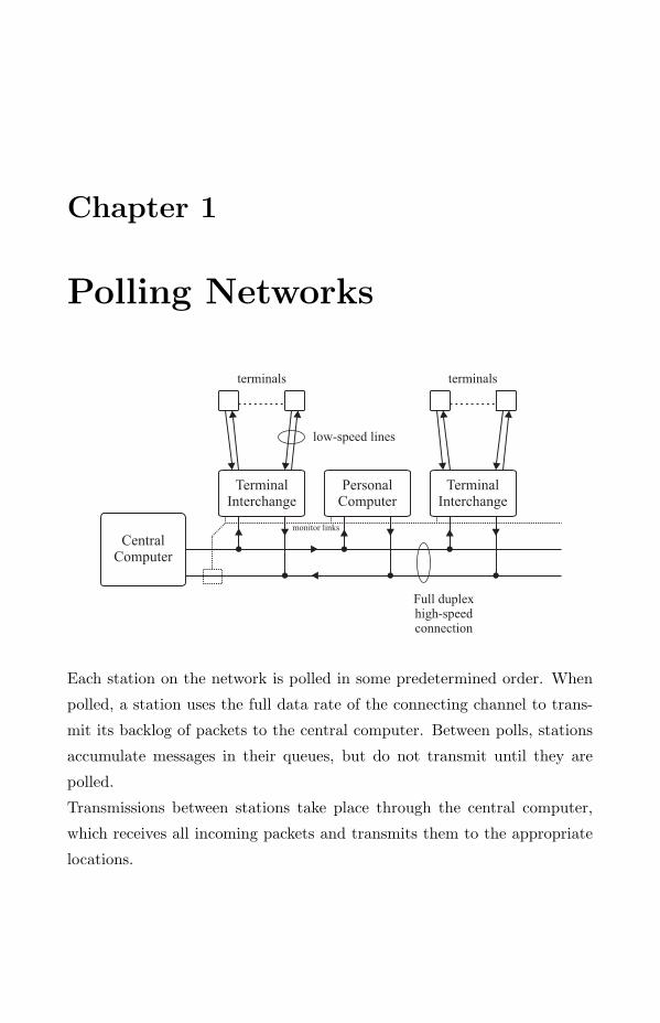
Each station on the network is polled in some predetermined order. When
polled, a station uses the full data rate of the connecting channel to trans-
mit its backlog of packets to the central computer. Between polls, stations
accumulate messages in their queues, but do not transmit until they are
polled.
Transmissions between stations take place through the central computer,
which receives all incoming packets and transmits them to the appropriate
locations.
EE414 Notes - Polling Mechanisms 2
Bit Sync CharacterSync.
Go-ahead StationAddress
CheckCharaters
End ofPacket
Go-ahead NextStation
Bit Sync CharacterSync.
TerminalAddress
StationAddress
CheckCharaters
End ofPacket
InformationContent
(a) Polling packet for roll-call polling
(b) Format for data packets
(c) Suffix to last data packet transmitted
Figure 1.1: Typical Packet Formats for Polling Network
1.1 Polling Mechanisms
Roll-Call Polling
Each station has to be polled in turn by the central computer (controller).
After the station has transmitted its backlog of messages, it notifies the
central controller with a suffix to its last packet. After receiving this suffix
packet, the controller sends a poll to the next station in the polling sequence.
Hub Polling
In this case the go-ahead (suffix) packet contains the next station address. A
monitoring channel must be provided to indicate to the appropriate station
that it should start transmitting. Essentially the go-ahead is transmitted
directly from one station to another.
1.2 Roll-Call Polling Operation
Station
• The central computer sends out a polling packet to station i in the
polling sequence.
EE414 Notes - Roll-Call Polling Operation 3
• Station i synchronises on bits and characters.
• Station i reads and interprets the station address and the go-ahead
contained in the polling packet.
• Station i transmits all its backlogged messages to the central computer
for distribution to the central computer and other stations.
• Station i appends a go-ahead, and possibly a next-station address to
its last packet.
Controller
• The central computer synchronises on bits and characters.
• The central computer reads and interprets the incoming packets, in-
cluding the final go-ahead and next station address.
• The central computer sends out a poll to station (i + 1).
These steps are repeated for each station. When all stations have been
polled the whole sequence begins again.
The communications between the controller and stations may be half-duplex
or duplex. We assume duplex.
Transmission from Controller to Stations: This can be asynchronous
or continuous. If continuous then step 2 of station operation can be ignored.
Transmission from Station to Controller: This is asynchronous. If
a station has no messages it either does not reply or sends back a go-ahead
packet.
EE414 Notes - Polling Analysis Model 4
1.3 Polling Analysis Model
Controller
Station 1
Station i
Station 2 Station M
Directionof Poll
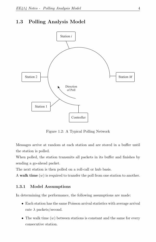
Figure 1.2: A Typical Polling Network
Messages arrive at random at each station and are stored in a buffer until
the station is polled.
When polled, the station transmits all packets in its buffer and finishes by
sending a go-ahead packet.
The next station is then polled on a roll-call or hub basis.
A walk time (w) is required to transfer the poll from one station to another.
1.3.1 Model Assumptions
In determining the performance, the following assumptions are made:
• Each station has the same Poisson arrival statistics with average arrival
rate λ packets/second.
• The walk time (w) between stations is constant and the same for every
consecutive station.
EE414 Notes - Polling Analysis Model 5
• The channel propagation times between stations are equal and are
included in the walk time.
• Packet length distributions are the same for packets arriving at each
station.
1.3.2 Average Cycle Time
Let:
Nm = Average number of packets stored at a station when poll arrives
X = Average length of packet (in bits)
R = Speed of transmission channel (in bits per second)
NmX/R = Time needed to empty station buffer (in seconds)
The next stations starts transmitting after the walk time w.
Length of average cycle time =
Tc = M [NmX/R + w]
where M is the number of stations.
From the input statistics:
Nm = λTc
Combining this with the previous equation to eliminate Nm gives:
Tc =Mw
1 − MλX/R
Define throughput S = MλX/R
Therefore:
Tc =Mw
1 − Sseconds
S must be < 1 in order to have finite buffer lengths at stations.
EE414 Notes - Polling Analysis Model 6
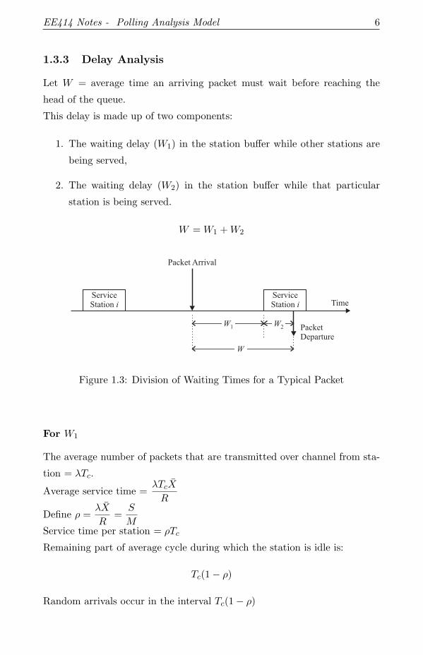
1.3.3 Delay Analysis
Let W = average time an arriving packet must wait before reaching the
head of the queue.
This delay is made up of two components:
1. The waiting delay (W1) in the station buffer while other stations are
being served,
2. The waiting delay (W2) in the station buffer while that particular
station is being served.
W = W1 + W2
ServiceStation i
ServiceStation i
Packet Arrival
PacketDeparture
W1
W
W2
Time
Figure 1.3: Division of Waiting Times for a Typical Packet
For W1
The average number of packets that are transmitted over channel from sta-
tion = λTc.
Average service time =λTcX
R
Define ρ =λX
R=
S
MService time per station = ρTc
Remaining part of average cycle during which the station is idle is:
Tc(1 − ρ)
Random arrivals occur in the interval Tc(1 − ρ)
EE414 Notes - Polling Analysis Model 7
On average the delay is:
Tc(1 − ρ)
2seconds
Using the previous expression for Tc:
W1 =Mw(1 − ρ)
2(1 − Mρ)
ServiceStation i+1
(1- )Tcñ ñTc
wServiceStation i
ServiceStation1
wService
Station MServiceStation i
Tc
Figure 1.4: A Cycle for a Polling Network, with Average Time Indicated
For W2
An approximation is used. Consider an equivalent network for which there
is no walk time so that there is always some station being served if there are
packets in the network.
Think of the whole system as having input Mλ and only a single server. An
M/G/1 model will apply.
The delay in a buffer for an M/G/1 system is:
W ′ =λ′
2(1 − ρ′)E[τ2]
where E[τ2] = σ2 + 1/µ2 is the 2nd moment of the service time distribution.
In our case
λ′ = Mλ
ρ′ = Mρ = S
E[τ2] =
[
X
R
]2
=X2
R2
EE414 Notes - Polling Analysis Model 8
Therefore
W2 =Mλ(X2/R2)
2(1 − S)=
MλX
R
1
2(1 − S)
1
XRX2
As S = MλX/R
W2 =SX2
2XR(1 − S)
Total delay is W1 + W2 so
W =Mw(1 − ρ)
2(1 − Mρ)+
SX2
2XR(1 − S)
Rewriting, the average time a packet must wait before reaching the head of
the queue in a polling network is:
W =Mw(1 − S/M)
2(1 − S)+
SX2
2XR(1 − S)
Two distributions of packet lengths are of interest:
Constant: X2 = (X)2
W =Mw(1 − S/M)
2(1 − S)+
SX
2R(1 − S)
Exponential: X2 = 2(X)2
W =Mw(1 − S/M)
2(1 − S)+
SX
R(1 − S)
EE414 Notes - Polling Network Example 9
1.4 Polling Network Example
Consider a metropolitan area network with a single central processor located
at the headend of a broadband CATV system that has a tree topology. The
following are specified:
• Maximum distance from headend to a subscriber station - 20 km
• Access technique - roll-call poling
• Length of polling packet - 8 bytes
• Length of go-ahead - 1 byte
• Data rate of channel - 56 kbps
• Number of subscribers - 1000
• Packet length distribution (subscriber to headend) - exponential
• Mean packet length - 200 bytes
• Propagation delay - 6 µs/km
• Mode of transmission - duplex
• Modem synchronisation time (at headend) - 10 ms
(a) Find the mean waiting time (delay) for arriving packets at the stations
if each user generates an average of one packet per minute.
(b) If the channel data rate is reduced to 9,600 bps, what is the largest
possible mean packet length that will not overload the system.
(c) For mean packet lengths of 2/3 the result found for (b), determine the
mean waiting delay.
First determine walk time (w). This is made up of:
• Tx time for go-ahead
• Propagation delay of go-ahead
EE414 Notes - Polling Network Example 10
• Tx delay for polling packet
• Propagation delay for polling packet
• Sync. delay of modem for received data at headend
Calculating these:
• 8/(56 × 103) = 0.14 ms
• 20 × 6 = 120µs = 0.12 ms
• 8 × 8/(56 × 103) = 1.14 ms
• 0.12 ms
• 10 ms
Total = 11.52 ms.
(a) Throughput per station
= ρ =λX
R=
1/60 × 200 × 8
56 × 103= 4.76 × 10⁻⁴
Total throughput
= S = Mρ = 1000 × 4.76 × 10−4 = 0.476
Mean Delay
= W =Mw(1 − S/M)
2(1 − S)+
SX
R(1 − S)
W =1000(11.52 × 10⁻³)(1 − 4.76 × 10⁻⁴)
2(1 − 0.476)+
0.476 × 200 × 8
56 × 103(1 − 0.476)
= 10.99 + 0.026 = 11.02 sec
(b)
SMAX =1000(1/60 × 8 × XMAX)
9600< 1
XMAX < 72 bytes
EE414 Notes - Polling Network Example 11
(c)
X = 2/3 × 72 = 48 bytes
throughput per station = ρ =λX
R=
1/60 × 48 × 8
9600= 6.67 × 10⁻⁴
total throughput =
S = Mρ = 1000 × 6.67 × 10−4 = 0.67
Polling packet and go-ahead transmission times change because of the new
channel bit rate. New walk time is given by:
w =8 × 8
9.6+
8
9.6+ 2 × 0.12 + 10 = 17.74 ms
Therefore W is given by:
W = 26.62 + 0.01 = 26.63 sec
Note that W in both cases is dominated by W1 (W2 ≈ 0).
Chapter 2
Ring Networks
station
ringinterface
unit
Figure 2.1: A Typical Ring Structure
A ring network is characterised by a sequence of point-to-point links between
stations, forming a loop. All messages travel in one direction around the
loop, passing through network interfaces at each station.
2.1 Operation of Ring
Bits from the ring enter in one direction in a serial fashion and, after a delay
of several bits, are retransmitted over the ring either unchanged, or after
some modification.
EE414 Notes - Operation of Ring 13
Access to the ring for transmissions in controlled by a token. A station
wishing to transmit waits for an idle token to arrive. It then changes it into
a busy token and follows it with data. An idle token is transmitted at the
end of the holding time.
In the listen mode, each station passes on the packet received at its input
after a delay referred to as the station latency. Define:
Ring Latency = Station Latency + Propagation Delay
The operational mode of a ring is determined by when idle tokens may be
generated. The modes are:
• Multiple-Token
• Single-Token
• Single-Packet
EE414 Notes - Operation of Ring 14
Line Driver Controller Line Receiver
Receiver Transmitter
Transmit Buffer Receive Buffer
Attached Device
Delay
RingInput
RingOutput
Nodein
Nodeout
Nodein
Nodeout
Listen Mode
RingInput
RingOutput
Delay
Nodein
Nodeout
Transmit Mode
RingInput
RingOutput
Figure 2.2: Station / Ring Interface
EE414 Notes - Operation of Ring 15
Figure 2.3: Operational Modes of Ring
EE414 Notes - Delay Analysis for Token Ring Networks 16
2.2 Delay Analysis for Token Ring Networks
The following assumptions are made in the analysis:
• All stations behave the same.
• The arrival process at each station is Poisson with average arrival rate
of λ.
• The average distance between the sending and receiving station is 1
2
the distance around the ring.
• The stations are spaced so that the propagation delays between con-
secutively serviced stations are equal and given by τ/M , where τ is
the total ring propagation delay and M is the number of stations.
• The packet length distribution is the same for each station with mean
length X bits and second moment X2.
• All packets queued at a station are transmitted during a service period.
Let:
R = Channel bit rate (bits/sec)
B = Latency per station (bits)
τ = Round trip propagation delay for the ring (sec)
τ ′ = Ring Latency (sec)
A common channel is used for both a token ring network and a polling
network. The master controller is not of importance to the operation of the
system in so far as the analysis is concerned. Thus, the polling equations,
developed in the previous chapter, can be used for token ring analysis.
The average waiting time in a polling network was derived to be:
W =Mw(1 − S/M)
2(1 − S)+
S(X/R)2
2(X/R)(1 − S)
The average transfer delay T is given by
T = X/R + τavg + W
EE414 Notes - Delay Analysis for Token Ring Networks 17
where
X/R = Average time to transmit a packet
τavg = Average latency from Tx station to Rx station
We need to state what τavg is for a token ring LAN.
We assume that a packet travels on average half way around the ring before
it reaches its destination station.
τ ′ = τ + MB/R
and τavg = τ ′/2.
The expression for W must be determined for token ring operation. Need
to evaluate:
1. The walk time (w)
2. Moments of the service time X/R and X2/R2
3. The network throughput
1. Walk Time
w = τ ′/M = B/R + τ/M
2. Service Time
For ring networks, the service time can include any time interval during
which the ring is inactive in the course of completing one packet transmis-
sion and becoming available for another transmission. Call this time the
Effective Service Time E.
3. Network Throughput
define S′ = MλE
while S = MλX/R
EE414 Notes - Delay Analysis for Token Ring Networks 18
Using these expressions gives
T =X
R+
τ ′
2+
τ ′(1 − S′/M)
2(1 − S′)+
S′E2
2E(1 − S′)
This gives a general expression for the delay in a token ring network. The
expressions for E, E2 and S′ will depend on the operational mode of the
ring and the packet length distribution.
Note that T is normally referred to as the unnormalised delay. The nor-
malised delay is defined as:
T =T
(X/R)
EE414 Notes - Multiple Token Operation 19
2.3 Multiple Token Operation
In this case a new token is generated immediately after the last bit of the
packet leaves the transmitting station. This is similar to the polling case as
the ring is always transmitting between walk times.
The average effective service time is X/R and the second moment is X2/R2.
Average transfer delay is therefore:
T =X
R+
τ ′
2+
τ ′(1 − S/M)
2(1 − S)+
SX2
2XR(1 − S)
Maximum throughput is obtained when S = 1. However S = 1 ⇒ T → ∞
which is not desirable.
For fixed length and exponentially distributed packet lengths we have: