C:/Documents and Settings/Robin Haskins/Desktop/slides/ch6 ...

Discrete Random Variables

Discrete-Event Simulation:A First Course

Section 6.1: Discrete Random Variables

Section 6.1: Discrete Random Variables Discrete-Event Simulation c©2006 Pearson Ed., Inc. 0-13-142917-5


Section 6.1: Discrete Random Variables

A random variable X is discrete if and only if its set ofpossible values X is finite or, at most, countably infinite

A discrete random variable X is uniquely determined by

Its set of possible values XIts probability density function (pdf):A real-valued function f (·) defined for each x ∈ X as theprobability that X has the value x

f (x) = Pr(X = x)

By definition,∑

x

f (x) = 1



Examples

Example 6.1.1 X is Equilikely(a, b)

|X | = b − a + 1 and each possible value is equally likely

f (x) =1

b − a + 1x = a, a + 1, . . . , b

Example 6.1.2 Roll two fair face

If X is the sum of the two up faces, X = {x |x = 2, 3, . . . , 12}From example 2.3.1,

f (x) =6 − |7 − x |

36x = 2, 3, . . . , 12



Example 6.1.3

A coin has p as its probability of a head

Toss it until the first tail occurs

If X is the number of heads, X = {x |x = 0, 1, 2, ...} and thepdf is

f (x) = px(1 − p) x = 0, 1, 2, ...

X is Geometric(p) and the set of possible values is infinite

Verify that∑

xf (x) = 1:

∑

x

f (x) =∞∑

x=0

px(1−p) = (1−p)(1+p+p2+p3+p4+· · · ) = 1



Cumulative Distribution Function

The cumulative distribution function(cdf) of the discreterandom variable X is the real-valued function F (·) for eachx ∈ X as

F (x) = Pr(X ≤ x) =∑

t≤x

f (t)

If X is Equilikely(a, b) then the cdf is

F (x) =

x

t=a

1/(b − a + 1) = (x −a+1)/(b−a+1) x = a, a+1, . . . , b

If X is Geometric(p) then the cdf is

F (x) =

x

t=0

pt(1−p) = (1−p)(1+p+· · ·+p

x) = 1−px+1

x = 0, 1, 2, ...



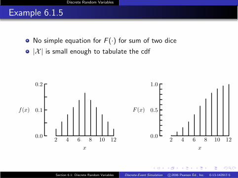
Example 6.1.5

No simple equation for F (·) for sum of two dice

|X | is small enough to tabulate the cdf

2 4 6 8 10 12

x

0.0

0.1

0.2

f(x)

2 4 6 8 10 12

x

0.0

0.5

1.0

F (x)



Relationship Between cdfs and pdfs

A cdf can be generated from its corresponding pdf byrecursion

For example, X = {x |x = a, a + 1, ..., b}

F (a) = f (a)

F (x) = F (x − 1) + f (x) x = a + 1, a + 2, ..., b

A pdf can be generated from its corresponding cdf bysubtraction

f (a) = F (a)

f (x) = F (x) − F (x − 1) x = a + 1, a + 2, ..., b

A discrete random variable can be defined by specifying eitherits pdf or its cdf



Other cdf Properties

A cdf is strictly monotone increasing:

if x1 < x2, then F (x1) < F (x2)

The cdf values are bounded between 0.0 and 1.0

Monotonicity of F (·) is the basis to generate discrete randomvariates in the next section



Mean and Standard Deviation

The mean µ of the discrete random variable X is

µ =∑

x

xf (x)

The corresponding standard deviation σ is

σ =

√∑

x

(x − µ)2f (x) or σ =

√√√√

(∑

x

x2f (x)

)

− µ2

The variance is σ2



Examples

If X is Equilikely(a, b) then the mean and standard deviationare

µ =a + b

2and σ =

√

(b − a + 1)2 − 1

12

When X is Equilikely(1, 6), µ = 3.5 and σ =√

3512

∼= 1.708

If X is the sum of two dice then

µ =

12∑

x=2

xf (x) = 7 and σ =

√√√√

12∑

x=2

(x − µ)2f (x) =√

35/6 ∼= 2.415



Another Example

If X is Geometric(p) then the mean and standard deviation are

µ =∞∑

x=0

xf (x) =∞∑

x=1

xpx(1 − p) = · · · =p

1 − p

σ2 =

(∞∑

x=0

x2f (x)

)

− µ2 =

(∞∑

x=1

x2px(1 − p)

)

− p2

(1 − p)2

...

σ2 =p

(1 − p)2

σ =

√p

(1 − p)



Expected Value

The mean of a random variable is also known as the expectedvalue

The expected value of the discrete random variable X is

E [X ] =∑

x

xf (x) = µ

Expected value refers to the expected average of a largesample x1, x2, . . . , xn corresponding to X : x̄ → E [X ] = µ asn → ∞.

The most likely value x (with largest f (x)) is the mode, whichcan be different from the expected value



Example 6.1.10

Toss a fair coin until the first tail appears

The most likely number of heads is 0

The expected number of heads is 1

0 occurs with probability 1/2 and 1 occurs with probability1/4

The most likely value is twice as likely as the expected value

For some random variables, the mean and mode may be thesame

For the sum of two dice, the most likely value and expectedvalue are both 7



More on Expectation

Define function h(·) for all possible values of X

h(·) : X → YY = h(X ) is a new random variable, with possible values YThe expected value of Y is

E [Y ] = E [h(X )] =∑

x

h(x)f (x)

Note: in general, this is not equal to h(E [X ])



Example 6.1.11

If y = (x − µ)2 with µ = E [X ],

E [Y ] = E [(X − µ)2] =∑

x

(x − µ)2f (x) = σ2

If y = x2 − µ2,

E [Y ] = E [X 2−µ2] =∑

x

(x2−µ2)f (x) =

(∑

x

x2f (x)

)

−µ2 = σ2

So that σ2 = E [X 2] − E [X ]2

E [X 2] ≥ E [X ]2 with equality if and only if X is not reallyrandom



Example 6.1.12

If Y = aX + b for constants a and b,

E [Y ] = E [aX+b] =∑

x

(ax+b)f (x) = a

(∑

x

xf (x)

)

+b = aE [X ]+b

Suppose

X is the number of heads before the first tailWin $2 for every head and let Y be the amount you win

The possible values Y you win are defined by

y = h(x) = 2x x = 0, 1, 2, . . .

Your expected winnings are

E [Y ] = E [2X ] = 2E [X ] = 2



Discrete Random Variable Models

A random variable is an abstract, but well defined,mathematical object

A random variate is an algorithmically generated possiblevalue of a random variable

For example, the functions Equilikely and Geometric

generate random variates corresponding to Equilikely(a, b)and Geometric(p) random variables, respectively



Bernoulli Random Variable

The discrete random variable X with possible valuesX = {0, 1}X = 1 with probability p and X = 0 with probability 1 − p

The pdf: f (x) = px(1 − p)1−x for x ∈ XThe cdf: F (x) = (1 − p)1−x for x ∈ XThe mean: µ = 0 · (1 − p) + 1 · p = p

The variance: σ2 = (0 − p)2(1 − p) + (1 − p)2p = p(1 − p)

The standard deviation: σ =√

p(1 − p)



Bernoulli Random Variate

To generate a Bernoulli(p) random variate

Generating a Bernoulli Random Variate

if (Random()< 1.0-p)

return 0;

else

return 1;

Monte Carlo simulation that uses n replications to estimate anunknown probability p is equivalent to generating an iidsequence of n Bernoulli(p) random variates



Example 6.1.14

Pick-3 Lottery: pick a 3-digit number between 000 and 999

Costs $1 to play the game and wins $500 if a player matchesthe 3-digit number chosen by the state

Let Y = h(X ) be the player’s yield

h(x) =

{

−1 x=0

499 x=1

The player’s expected yield is

E [Y ] =1∑

0

h(x)f (x) = h(0)(1 − p) + h(1)p = · · · = −0.5



Binomial Random Variable

A coin has p as its probability of a head and toss this coin ntimes

Let X be the number of heads; X is a Binomial(n, p) randomvariable

X = {0, 1, 2, · · · , n} and the pdf is

f (x) =

(nx

)

px(1 − p)n−x x = 0, 1, 2, · · · , n

n tosses of the coin generate an iid sequence X1, X2, · · · , Xn

of Bernoulli(p) random variables and X = X1 + X2 + · · · + Xn



Verify that∑

x f (x) = 1

Binomial equation

(a + b)n =n∑

x=0

(nx

)

axbn−x

In the particular case where a = p and b = 1 − p

1 = (1)n = (p + (1 − p))n =n∑

x=0

(nx

)

px(1 − p)n−x



Mean and Variance of Binomial(n, p)

The mean is

µ = E [X ] =n∑

x=0

xf (x) =n∑

x=0

x

(nx

)

px(1 − p)n−x

= npn∑

x=1

(n − 1)!

(x − 1)!(n − x)!px−1(1 − p)n−x

Let m = n − 1 and t = x − 1

µ = np

m∑

t=0

m!

t!(m − t)!pt(1−p)m−t = np(p+(1−p))m = np(1)m = np

The variance is

σ2 = E [X 2] − µ2 =

(n∑

x=0

x2f (x)

)

− µ2 = · · · = np(1 − p)



Pascal Random Variable

A coin has p as its probability of a head and toss this coinuntil the nth tail occurs

If X is the number of heads, X is a Pascal(n, p) randomvariable

X={0,1,2,...} and the pdf is

f (x) =

(n + x − 1

x

)

px(1 − p)n x = 0, 1, 2, ...



Pascal Random Variable ctd.

Negative binomial expansion:

(1−p)−n = 1+

(n1

)

p+

(n + 1

2

)

p2+· · ·+(

n + x − 1x

)

px+· · ·

Prove that the infinite pdf sum converges to 1

∞∑

x=0

(n + x − 1

x

)

px(1 − p)n = (1 − p)n(1 − p)−n = 1

It can also be shown that

µ = E [X ] =∞∑

x=0

xf (x) = · · · =np

1 − p

σ2 = E [X 2] − µ2 =

(∞∑

x=0

x2f (x)

)

− µ2 = · · · =np

(1 − p)2



Example 6.1.17

If n > 1 and X1, X2, ...,Xn is an iid sequence of nGeometric(p) random variables, the sum is a Pascal(n, p)random variable

For example,if n = 4 and p is large, a head/tail sequencemight be

hhhhhht︸︷︷︸

X1=6

hhhhhhhhht︸︷︷︸

X2=9

hhhht︸︷︷︸

X3=4

hhhhhhht︸︷︷︸

X4=7

X = X1 + X2 + X3 + X4 = 26

We see that a Pascal(n, p) random variable is the sum of iidGeometric(p) random variables



Poisson Random Variable

Poisson(µ) is a limiting case of Binomial(n, µ/n)

Fix µ and x as n → ∞

f (x) =n!

x!(n − x)!

µ

n

x

1 −

µ

n

n−x

=µx

x!

n!

(n − x)!(n − µ)x1 −

µ

n

n

It can be shown that

limn→∞

n!

(n − x)!(n − µ)x= 1 and lim

n→∞

1 −

µ

n

n

= exp(−µ)

So that

limn→∞

f (x) =µx

x!exp(−µ)


Date post:	31-Dec-2021
Category:	Documents
Upload:	others
View:	3 times
Download:	0 times