IAQF Academic CaseFinal Project Report

CDS on CDO PortfolioA Fundamental Factors’ Model forHedging, Collateralization and Capital ReservesTIME SQUARED EXPLORERS

AbstractIn this study, we have identified the cause of AIG’s failure in 2008 to be large unhedged CDS exposures on CDO portfolios.We built a fundamental factors model to price CDS-CDOs as well as create hedging strategies. We specified subprimemortgage default and prepayment hazard rates to be dependent on common fundamental factors including interest rates andhousing prices as well as deal specific idiosyncratic factors. We calibrated our base fundamental factor parameters withloan level ARM mortgages and make certain assumptions for the CDOs. We then studied the hedging performance withinstruments like ABX.HE indicies, Euro dollar futures and Home Price Index futures. We propose a new collateral schemebased on CVA values of both counter- parties. We also demonstrate a framework to calculate the VaR on the CVA andexpected loss distributions of the CDS after col-lateralization. We then propose a method to determine the capital reserveneeded for CDS contracts based on two VaRs.

KeywordsFundamental Factors, Hedging, Collateralization, Capital Reserve, CDS-CDOs

Contents

1 Introduction 1

2 A Reflection on How AIG Collapse 12.1 AIG Bail-out Recap . . . . . . . . . . . . . . . . . . . . . . . 12.2 Cause I: Gigantic Unhedged Exposure . . . . . . . . . . 22.3 Cause II: Problematic Credit Annex Support . . . . . . . 22.4 Moral Hazard of the Bailout . . . . . . . . . . . . . . . . . . 3

3 Fundamental Factor Model 43.1 Factors Specifications . . . . . . . . . . . . . . . . . . . . . 43.2 From Factors to Cash Flows of Mortgages . . . . . . . . 43.3 From Mortgage Pool to MBS Cash Flows . . . . . . . . . 5

4 Cross Market Hedging of CDS-CDOs 54.1 Hedging with ABX.HE Indexes . . . . . . . . . . . . . . . 54.2 Hedging with Interest Rate Futures and HPI Futures . 64.3 Hedging with Puts on Equity . . . . . . . . . . . . . . . . . 7

5 CVA-based Collateral Agreement 85.1 Collateral, The Economics Behind . . . . . . . . . . . . . 85.2 Implementation of CVA . . . . . . . . . . . . . . . . . . . . 9

6 Capital Reserve of CDS 10

7 Conclusion 11

1. Introduction

The near collapse of the American International Group (AIG),the largest insurance company by then, is one of the most se-vere events during the subprime-mortgage crisis. The bailout

of AIG, along with other concurrent collapses of some majorfinancial institutions, led both the practitioners and regula-tors to reflect upon their legacy risk management practices.Under the context of emphasis on deregulation and financialinnovations after Financial Services Modernization Act of1999 (FSMA) and the Commodity Futures Modernization Actof 2000 (CFMA), disputes had arisen over how to strike thebalance between the cost of carrying stringent risk manage-ment and regulatory burden and the benefits from rolling outstructured financial instruments in a more inter-related finan-cial system. Thereafter, we saw a market inclination towardsvanilla instruments. The new regulatory frameworks, DoddFrank Act and BASEL III accord (Basel Committee, 2010),both aim at ensuring the wellness of financial system.

In this study, we will revisit bailout of AIG, based on whichwe will propose a fundamental factor approach to mitigatethe risks of then AIG’s most problematic position - the creditdefault swap portfolio on collateralized debt obligations. Aswe shall see later, our factor approach will consistently offerthree layers defense - hedging, collateral management andcapital reserve - each of which will address the an particularproblem of AIG’s collapse and roots deeply in the economics.The rest of the report is organized as follows

2. A Reflection on How AIG Collapse

2.1 AIG Bail-out Recap

AIG’s fall epitomizes the aforementioned issue and the ongo-ing debate on managing the complicated financial products. It

CDS on CDO PortfolioA Fundamental Factors’ Model for

Hedging, Collateralization and Capital Reserves — 2/14

is generally agreed that the AIG’s credit default swap portfolioon super-senior tranches of multi-sector collateralized debtobligations (CDS-CDOs) is the fatal cause of AIG’s “death”(Sjostrom Jr, 2009; Boyd, 2011). The disruption in the hous-ing market in 2007 seriously devalued the mortgages andmortgaged-based derivatives (American International Group,2007, 2008). Through both direct investments in RMBS andthe CDS-CDOs position, AIG maintained a gigantic expo-sure to mortgage market and hence had to record billions ofrealized and unrealized losses. Questioning the AIG’s abil-ity to fulfill the obligations, counter-parties to AIG initiatedcollateral calls one after another, resulting demand of liquidassets amounting to more than 50 billions - a disastrous num-ber that pushed AIG towards the verge of bankruptcy whichwas avoided only after the Federal Reserve put together $85billion credit facility to bail out AIG (Sjostrom Jr, 2009)

However, it is inaccurate to solely attribute the consequenceto CDS-CDOs or the abrupt decline of housing market. Thedesign of the CDS aims to benefit from risk diversification andrisk transferring through securitization (Lucas et al., 2007).CDS arose from the need of credit risk protection. Both ofthese instruments, in theory, are to achieve better risk alloca-tion among players in financial market. As long as the risksare priced appropriately to compensate the firms who bearthe risk, nothing is economically wrong with the CDS-CDOsitself. Hence, AIG fell not because they maintained a CDS-CDOs portfolio on their book but rather they took on riskswhich exceed their capabilities to manage effectively:

2.2 Cause I: Gigantic Unhedged Exposure

Firstly, the most identifiable problem is AIG’s gigantic expo-sure to the mortgage market through both direct investmentsand the unfunded CDS portfolios. Since AIG dabbled theCDS business in 1998 through its subsidiary called AIG Fi-nancial Products (AIGFP), AIG gradually became the majorprotection seller in the market, mainly due to AIGFP’s AAAcredit ratings inherited from AIG via the contractual guar-antee agreement (TPM, 2009). Such a AAA-rating businessmodel enabled AIGFP to price its CDS competitively andaccumulate market share quickly.

Throughout early 2000s when market was deregulated andfinancial innovations were encouraged, AIGFP had expandedits CDS coverage extensively from conventional corporatebonds to more exotic OTC contracts on CDO. According toAmerican International Group (2007), by the end of 2007,AIGFPs CDS position was as large as $527 billion, which wasquickly increased from $203 billion in 2003. Among the $527billion, $378 billion was sold to mainly European banks withthe purpose to reduce the capital requirements (“RegulatoryCapital Relief”) and the $149 billion, including the toxic $78billion protection on CDOs, was contracted with the clients,such as Goldman Sachs, who were interested then popularnegative-basis arbitrage (“Arbitrage Portfolio”) (American

International Group, 2008).

Such a position, with hindsights, was too large given thatAIG had only 2.3 billion in cash and $95 billion in equity toabsorb the losses. The question on their capability to handlethe big position was even more confounded as AIG directlyinvested in mortgage securities in its ordinary business andsecurities lending program (Sjostrom Jr, 2009). Yet, as writtenin AIG’s 2007 Annual report, the management decided not tohedge their position in CDS with the preconception that supersenior tranches are safe given their simulation and modifiedBET models. When the mortgage market did go against theirbet, the loss was significant in a sense that CDS-CDOs solelycontributed a $11.2 and $25.7 billion unrealized loss in 2007and 2008, in addition to other realized impairment cost ($20 -$30 billion) in 2008 (American International Group, 2008).

However, had AIG intended to hedge the position some timebefore the financial crisis, situation would possibly not bemore favorable to AIG. CDS are insurance-like contracts.As CDS is the most common and thus the cheapest sourcesof credit protection, it would be difficult to look for cheapalternatives to remove exposure from CDS. This is especiallytrue when (1) the secondary market of both the reference assetand the CDS are not liquid enough, and (2) reinsurance marketis not large. To cut or hedge billions of exposure in any marketduring distressed time was intrinsically hard, not to mentiontheir contracts are mostly OTC. Hence, perhaps, AIG shouldhave not put itself into a huge CDO pool at first.

2.3 Cause II: Problematic Credit Annex Support

The second problem, which is also the feature that differen-tiates the CDS-CDOs position from other direct mortgageinvestments, is the collateral posting obligations embedded tothe CDS contracts. Such type of obligations imposes contin-gent demand on the firms liquidity and, in contrary to the assetdevaluation, the inability to fulfill the cash obligation will leadto the immediate bankruptcy of the firm. After Goldman Sachscollateral calls as the CDO market worsened, major counter-parties to AIG started following the practices, putting AIGinto cash woes. The subsequent downgrade of AIG automati-cally applied another multiplicative factor to the already-hugecollateral base. By September 2008, AIG was required to postalmost $31 billion collateral solely against CDS on CDOspositions (American International Group, 2009). Adding thecollateral from security lending business GIA, the numberwas as high as $54 billion - an amount was filled only afterFed stepped in (Sjostrom Jr, 2009; Boyd, 2011)

The collateral crisis on one hand was the result of managementnegligence but, fairly speaking, the terms of the Credit SupportAnnexes itself made collateral management difficult for AIG.According to AIG’s FY2008 10-K, the calculation of collateraldelivery amount against CDS-CDOs position is a two-stepprocess

CDS on CDO PortfolioA Fundamental Factors’ Model for

Hedging, Collateralization and Capital Reserves — 3/14

1. Determine the exposure: computed as the differencebetween the net notional amount and the market valueof the underlying CDOs;

2. Determine the delivery amount: the collateral to bedelivery equals the net exposure which is the exposureless the collateral which has already been posted.

In additional to the above framework, AIG is allowed to

• post no collateral when the underlying CDO loss isbelow certain threshold, typically 4% as those withGoldman Sachs.

• post less collateral with a multiplicative factor based onAIG’s credit ratings.

There are at least 4 potential problems associated with theaforementioned CSA. Firstly, instead of using the replacementvalue of the contract, the collateral is “market-price based”in which the “market value of relevant CDO security is theprice at which a marketplace participant would be willingto purchase such CDO security in a market transaction onsuch date”. For illiquid reference asset, such as CDO security,whether the market quote is the accurate proxy of the trueeconomic value of the asset is questionable. This is evidentespecially in distressed financial market. Stanton and Wallace(2011) shows that the ABX.HE index during the crisis wastraded extremely low, implying an unrealistic high default andlow recovery rate which have never been observed in GreatDepression. Collateral mechanism based on these marketinformation can be overly volatile due to the market sentiment.Moreover, collateral is to ensure the “payment of CDS whenreference actually default” instead of “hedging the value ofinstrument”. Marked-to-market at an extremely distressedmarket is overly stringent for AIG

Secondly, the mechanism of the collateral threshold and thedependency of the collateral amount on credit ratings directlyresulted in the risk of “jump in liquidity needs”. In otherwords, when the CDO market loss hit the threshold or creditratings lowered, the collateral call can often be sudden andlarge. Moreover, the unexpected cash needs often coincideswith financial distress which could lead to considerable diffi-culties in raising additional funds. Hence, such a jump can bedetrimental as the cash-based obligation is probably one of thehardest types of obligation to fulfill and leads to immediatedefault no matter how much assets the firm has on book.

Thirdly, the trigger rule, despite it appears to be beneficial toAIG, tends to hide the liquidity risk and lead managers to over-look the collateral management practices. The superseniortranches of CDOs were considered with really low defaultrisk before the crisis. Hence the super-senior tranches weretraded near par and AIG was not required to post collateralas CSA was not triggered. This induced the management toaccumulate large position while being unaware of the liquidityexposure, in that their position was almost free of cash burden.However, when the underlying asset goes bad, as in the case

of AIG, the liquidity risk can be too large to be managed.

Lastly, the CSA design is loosely related to the credit riskof both counter-parties and the variability of the underlying.On one hand, the determination of the collateral trigger ap-pears arbitrary and rigid over the life of the CDS contract. Onthe other hand, the infrequent adjustment of the credit ratingmeans the counter-party risks are not captured timely. Bothof the aforementioned disadvantages suggest the lack of eco-nomic interpretation of this CSA settings, veil the true natureof counter-party risk and hence make the collateral hard tomanage.

2.4 Moral Hazard of the Bailout

The FRBNY thought it would be unethical to leverage thisthreat of bankruptcy, since it knew it was not willing to letAIG default. By imposing onerous conditions to the $85billion RCF, the Fed did a good job of minimizing the micromoral hazard in the short run. Unfortunately, this did signalthat they were not willing to let AIG default, which ultimatelyled to the much larger moral hazard of bailing out the AIGcounterparties.

As acknowledged by Fed Vice Chairman Donald Kohn at aSenate Banking Committee hearing, the aid to these coun-terparties contributed to moral hazard and “will reduce theirincentive to be careful in the future”. The fact that the coun-terparties did not take a haircut has been widely criticized,including by Neil Barofsky, the former inspector general ofthe Troubled Asset Relief Program (TARP). Barofsky toldcongress that “No lessons were learned from the counterpar-ties, other than, if you do business with a giant, too-big-to-failinstitution, you don’t need to worry about it because UncleSam is going to sit there and backstop all of your bad bets.”1

This could led to a market distortion where investors, creditorsand counterparties don’t bother with due diligence of theselarge, interconnected financial institutions, which in turn couldlead to lower borrowing costs for these financial institutions.According to Senator Elizabeth Warren2, the Too-Big-to-Failproblem has in fact gotten worse since the financial crisis. Ina speech promoting the 21st Century Glass-Steagall Act, shesaid

Today, the four biggest banks are 30% largerthan they were five years ago. And the five largestbanks now hold more than half of the total bank-ing assets in the country. One study earlier thisyear showed that the Too-Big-to-Fail status is giv-ing the 10 biggest U.S. banks an annual taxpayersubsidy of $83 billion.

1Quote retrieved from http://hereandnow.wbur.org/2013/09/13/tarp-watchdog-banks

2Quote Retrieved from https://www.commondreams.org/headline/2013/11/12-11

CDS on CDO PortfolioA Fundamental Factors’ Model for

Hedging, Collateralization and Capital Reserves — 4/14

3. Fundamental Factor Model

The aforementioned analysis of fall of AIG’s suggests that atleast three lines of defense can be establish to mitigate, if notavoid, the downside risk of huge mortgage position. The firmshould (1) reduce the exposure by either trimming the positionor hedging the losses, which could avoid the abrupt loss ofcredibility and hence maintain the funding capabilities in adisrupted market; (2) establish a better collateral agreementthat will facilitate a better understanding of credit exposureand collateral management, and (3) set aside adequate amountof firm-wide capital to serve as the last defense should theabove trade-specific risk management fails.

However, as the protection seller of bond, looking for otheralternatives to directly short the credit risk is difficult, asCDS is already the cheapest credit instrument. Hence, toavoid enormous hedging cost, especially when hedging largeposition, cross hedging tends to be a more feasible solution.Candidates of these instruments are the housing price index,ABX indices as well as the put options on firms which haveexposure to mortgage market. These choices are based onthe economic reasoning that the dynamics of these assets aremore or less driving by the mortgage market.

3.1 Factors Specifications

This idea suffices the use of fundamental factor model insteadof the common statistical model, such as copula or BET. Thefundamental models can identify inherent risks and establishsound hedges. Specifically, we assume that the economyof mortgages are primary driven by housing price (housingindex) and the interest rate. Mathematically, we adopted thelog-normal model to capture the dynamics of the housingprices

dHt = (rt −qt)Ht +σHdW1 (1)

and the interest rate rt is given using the one-factor Hull-Whitemodel (Hull and White, 1993).

drt = κ(θt − rt)rt +σRdW2 (2)

where qt in equation (1) is the rental yield and assumed to bea constant qt = 0.25 following Downing et al. (2005); W1 andW2 are Wiener processes under risk-neutral measure and areassumed to be independent for simplicity. That is, we let

dW1dW2 = 0, qt = 0.25 ∀t > 0 (3)

3.2 From Factors to Cash Flows of Mortgages

Proportional Hazard Rate Model

It is known that the cash flows of mortgages and therebymortgage-backed securities heavily depends on the prepay-ment risk and default probability. To model the influenceof housing index and interest rate on mortgage payments,

we adopted the proportional hazard rate model proposed bySchwartz and Torous (1989) in which (1) prepayment / de-fault intensities are directly captured, and (2) the economicvariables are explicitly incorporated. Mathematically, eitherthe prepayment or the default hazard will follow

λ (t,Xi) = λ0(t)exp{β1X1 +β2X2 + · · ·+βnXn} (4)

where λ0(t) is the baseline hazard controlling the shape ofterm structure, and the linear combination of covariates Xi’sdetermines loan-specific shift of prepayment / default inten-sities. For the baseline hazard, we chose the log-logisticfunction

λ0(t;λ , p,γ) =λ p(λ t)p−1

1+(λ t)p (5)

The major benefits of such a functional form is its flexibilityin fitting a variety of shapes of prepayment or default pattern,such as the well-known burn-out phenomena of mortgages.

The selection of the covariates will determine how mortgagescash flows depend on the macro economy and the deal speci-fications. In this project, the following covariates are assumedin the proportional hazard rate models:

• Coupon Differential, which is defined as the differ-ence between the coupon on the loan and the 3-monthlagged 10-year interest rate. That is

X1(t) := CD(t) :=C−R(3) (6)

Large coupon differential induce mortgage borrowersto prepay the loan and refinance the mortgage wheninterest rate is low;

• Loan-to-Value Ratio, which is defined as

X2(t) := LTV(t) = Lt/Vt (7)

where Lt is the remaining principal of the loan at time tand Vt is the value of the property at time t. To modelthe dynamics of the property value, we further assumethat the return of Vt coincides with the return of housingindex

dVt

Vt=

dHt

Ht(8)

The two covariates only explains the the impact of the macro-economic factors on mortgage cash flows. However, eachloan pool can also be influenced by deal-specific variables,such as credit scores, property location etc. To account forthe idiosyncratic components, we add a time-varying “factor”to proxy the residual information. Mathematically, the “thirdfactor” takes the form

X3(t) := β0 + ε(t) ε(t)∼ i.i.d N(0,σ2) (9)

CDS on CDO PortfolioA Fundamental Factors’ Model for

Hedging, Collateralization and Capital Reserves — 5/14

and we further assume that the idiosyncratic factors are inde-pendent among deals. Combining the equation (6), (7), (9)with (4). Our modified hazard rate is

λ (t) = λ0(t)exp{β0+β1CD(t)+β2LTV(t)+ε(t)} (10)

which can be obtained through simulation when parameter iscalibrated.

Model Calibration

To calibrate the model, we used the mortgage loan-level data.With the hazard rate model above, we adopted the MLE toobtained the estimates.

Mortgage Cash Flows and Defaults

With the hazard rate term structure, λ (t), the prepayment orthe default probability in a given period is

PD(T1,T2) = exp{∫ T2

T1

λ (t)dt}≈ exp{λ (T2)(T2−T1)}

(11)

where the last term approximates the probability with a piece-wise constant hazard rate. Let PDP(t), PDD(t) denote theprepayment probability and the default probability respec-tively, then the mortgage payment can be computed throughthe following four steps (See Figure 12)

1. Given the last period ending balance L(t−1), we cancompute the average default amount of the mortgagepool with

Default(t) = L(t−1)×PDD(t)

2. Then the amortization math can be applied to the re-maining non-default balance of the bond to computethe principal and the interest portion of the payments.Denoted with P(t) and I(t) respectively.

3. After the amortization is determined, the prepaymentis obtained by applying PDP(t) to the balance after thedefault and principal payment are deducted c

Prepayment(t) = [L(t−1)−P(t)−Default(t)]×PDP(t)

4. The ending balance is then

L(t) = L(t−1)−P(t)−Default(t)−Prepayment(t)

Iterate the above four steps until the mortgage pools terminatewill gives us the default amount and the cash flows availablefor distribution for each period t.

3.3 From Mortgage Pool to MBS Cash Flows

Given the cash flows and the amount defaulted of the mort-gage pool, we can determine the cash flow that each tranchereceives based on the structure of the MBS. Here, for thesimplicity of illustration, we assume that all MBSs have asimple waterfall structure without the accrued interest class(Z), overcollateralization (X) and the residual class (R) whichare often observed in the real deals.

With the simple deal structure, as shown in Figure 12, cashflows are distributed according to the seniority of the tranches,with the most senior bond paid-off first. On the contrary, thedefault amount will cause the least senior tranche to be written-off first. Through this approach, the period-by-period cashflows and default amounts are obtained, based on which wecan model the cash flow of CDO and other mortgage relatedsecurities

4. Cross Market Hedging of CDS-CDOs

4.1 Hedging with ABX.HE Indexes

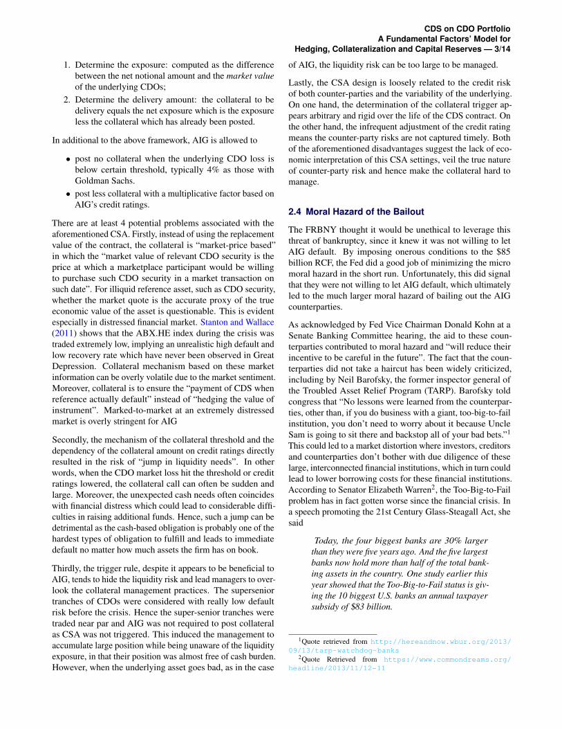
In this study, we simulated 100 MBS deals by modeling atpool level the cash flows of defaults and prepayments. TheMBS subordination structures are identical in those dealsas they are in table 1. We randomly selected 100 trancheswith 20 tranches from tranche 3 to 7 each and one tranchefrom each MBS deal to from a CDO. The CDO subordinationstructure is the same as the MBS deals. We performed the MCsimulation with 2000 interests and HPI paths, and analyzedthe joint distribution of the loss of the senior CDO tranche andthe average loss of the MBS tranches. The average losses fromthe MBS tranches were calculated from randomly selected 20deals. The CDO senior tranche incurred losses on 727 pathsof the 2000 paths.

Table 1. Subordination Level of the Representative Deal

Tranche Subordination (in %) Spread (in bps)

1 22.1 182 18.4 263 13.5 334 11.5 385 9.8 416 8.2 477 6.7 808 5.3 1009 4.2 200

From our simulation, we observed that the senior tranche ofthe CDO formed from equal numbers of tranche 3 to 7 of theMBS deals behaves generally in par with MBS tranche 3 and4. The CDO senior tranche loss cash flows are very similar tothose of the MBS tranche 3 and 4. They start to incur losses

CDS on CDO PortfolioA Fundamental Factors’ Model for

Hedging, Collateralization and Capital Reserves — 6/14

similarly. This is consistent with the diversification effectachieved with the CDO structuring. However, contrary tothe intention of most CDO deals in the reality, we found thesenior CDO tranche is inferior to the most senior tranche ofthe MBS deals. Our simulations results shows that the seniortranche of our CDO incurred about 50% loss before the mostsenior MBS tranche start to incur losses. This is likely due tothe fact we calibrated parameters with subprime loans withhigh default rates, therefore the junior tranches has higher losscorrelations, undermining the effect of diversification in theCDO deal.

In reality, a viable hedging strategy on the CDS on the seniortranche of CDO deal can be constructed as follows. First, thecash flows of the MBS deals are first modeled. This shouldbe preferably done in the loan level, utilizing as much as loanlevel information as possible. Then the cash flows to the CDO(and thus CDS) and the 20 ABX deals are simulated underthe same sets of scenarios. Their joint loss distributions areanalyzed, and corresponding ABX class with the highest losscorrelation should be chosen as the hedging instrument. In oursimulation, the average of MBS tranche 4 and 5 are arguablythe best hedging instruments, since they incur losses the samepoints with the senior CDO tranche and the expected losseshave linear relationship when they start to occur.

4.2 Hedging with Interest Rate Futures and HPI Fu-tures

Any financial instruments used to hedge large short CDSpositions should have the following desirable features:

1. the instrument should have minimal counterparty risk sothat the hedge does not fail in times of stress when largedefault payments need to be made. Given this consideration,we prefer exchange-traded instruments for hedging over over-the-counter instruments.

2. instruments used in dynamic trading strategies for hedginglarge positions should be highly liquid and have low bid-askspreads so that transactions cost is not prohibitive, and marketdoes not move against the trade. The inherent standardizationin exchange-traded contracts lends itself to this consideration.

We describe a dynamic hedging strategy in which the hedgeneeds to be rebalanced every period. Interest rates affect CDSprices in 2 different ways: 1. cash flows are discounted byinterest rates, and 2. default rate changes with interest ratedue to which cash flows from the CDS change. However, forCDS contracts, the default effect is expected to dominate thediscounting effect. Since ARM default rates increase as inter-est rates increase, we expect CDS value from seller’s point ofview to decrease when interest rate increases. Similarly, dur-ing a housing market boom, we expect default rate to decreasewhich would increase CDS value from seller’s point of view.

To obtain interest-rate duration and housing price index (HPI)duration of the CDS contract, we run a regression of the form

CDSi = α +β · ri + γ ·HPIi + εi

where i indexes Monte-Carlo paths, CDSi represents CDSMTM along path i at time t = 1, ri represents interest ratealong path i at time t = 1, HPIi represents housing price indexvalue along path i at time t = 1 and εi is the error term. Toavoid in-sample fitting bias, we only use half of our Monte-Carlo paths to generate this regression fit. Given estimatesfor the parameters α̂ , β̂ and γ̂ , our estimate for interest rateduration at time t = 0 is Dir

cds = −∂CDS

∂ r = −β̂ and for HPIduration at time t = 0 is Dhpi

cds = −∂CDS∂HPI = −γ̂ . Based on

our simulation, we obtain α̂ = 4.67 ∗ 106, β̂ = −4.29 ∗ 108,γ̂ = 2.33∗106 and R2 = 58.69%. The high negative value ofβ̂ and high positive value of γ̂ both make intuitive sense asdescribed previously. In Figure 1, we show a fit of actual CDSMTM at time t = 1 v/s estimated CDS MTM at time t = 1.

−3 −2 −1 0 1

x 107

−3

−2

−1

0

1

x 107

Estimated CDS Price (in $)

CD

S P

rice

(in $

)

Figure 1. Regression of Actual CDS MTM vs EstimatedCDS MTM

We now need to choose appropriate hedging instruments.Since a wide variety of exchange-traded interest rate con-tracts are available in the market, we run a regression betweeninterest rates and CDS prices at time t = 1 and notice a clearlinear relationship between the two. Hence, we choose CMEEurodollar futures as the interest rate hedging instrument.CME Eurodollar futures contracts are highly liquid standard-ized exchange traded contracts with almost no counterpartyrisk and are well-suited to act as a hedging instrument. SinceEurodollar future prices are given by 100− r, they have analmost linear exposure to interest rates and hence, are well-suited for hedging interest rate exposure of CDS. The notionalamount of Eurodollar futures to enter into is calculated asNir =−

Dircds

Dirf ut

= β̂ so as to make the hedge portfolio duration-

neutral.

CDS on CDO PortfolioA Fundamental Factors’ Model for

Hedging, Collateralization and Capital Reserves — 7/14

The regional diversification of mortgages underlying MBSand CDO instruments means that CDS instruments have ex-posure to US-wide housing market. As such, we choose CMEHousing Composite Index futures to hedge house price expo-sure in CDS contracts. For clarity, we describe contractualdetails of the instrument briefly below.

The S&P/Cash-Shiller home price indices are designed tobe a consistent benchmark of housing prices in the UnitedStates. They measure the average change in single-familyhome prices in a particular geographic market. The indicesare calculated with the repeat sales method, which uses data onproperties that have sold atleast twice, in order to capture thetrue appreciated value of constant quality homes. The mainvariable used for index construction is the price change be-tween two arms-length sales of the same single-family home.The S&P/Cash-Shiller National Home Price index is a com-posite of single-family home price indices for the nine USCensus divisions and is calculated quarterly (S&P Indices,2011).

The S&P/Cash-Shiller home price index is tradeable throughfutures on the Chicago Mercantile Exchange, known as Hous-ing Composite Index (HCI) Futures. These futures are cash-settled and the underlying is 250 times the S&P/Cash-ShillerNational Home Price index. Typically, contracts expiring dur-ing the next 6 quarters are available to trade at any given pointof time.

From empirical data, we observe that bid-ask spread for front-end expiring HCI Futures is approximately 4% of notional.Using trading volume data for 2012 and 2013, we observethat approximate annual trading volume is 300 contracts. Thebid-ask spread and annual volume most likely make HCIFutures infeasible as a hedging instrument but we hope thatgreater awareness, more quotes from other traders, and awillingness by traders and hedgers to dabble in these productswill improve liquidity of futures on this critically importantfinancial market. (Dolan, 2011)

Since HCI futures duration can be written as Dhpi(t)= exp((rt−q)∗ (T − t)), where q = dividend yield on HPI and T = settle-ment time of HCI future, we can calculate the notional amount

of HCI futures to enter into as Nhpi =−Dhpi

cdsDhpi

= exp(−(r0−q)∗T )∗ γ̂ . We obtain Nir =−4.29∗108 and Nhpi =−2.34∗106.

Finally, hedge portfolio MTM can be calculated as CDSHi =

CDSi +Nir ∗ IRMT Mi +Nhpi ∗HPIMT M

i , where IRMT Mi = MTM

of Eurodollar futures contract along path i at time t = 1 andHPIMT M

i = MTM of HCI futures contract along path i at timet = 1. We use the Monte-Carlo paths not used to calculatedurations to evaluate the performance of our hedge portfolioover the next period. We observe that 1. the standard deviationof MTM portfolio value at time t = 1 decreases from 8.02∗106 to 4.69 ∗ 106, and 2. we eliminate fat tails to quite alarge extent. The strategy described above can now be reusedto update the hedge portfolio at time t = 1. The Figure 2

shows the probability distribution of the hedged and unhedgedportfolio.

−3 −2 −1 0 1

x 107

0

0.02

0.04

0.06

0.08

0.1

0.12

Portfolio Value (in $)

Prob

abili

ty

UnhedgedHedged

Figure 2. Probability Distribution of Hedged and UnhedgedPortfolio Value

4.3 Hedging with Puts on Equity

AIG’s leveraged positions accumulated to a large exposure tothe mortgage market. The total credit exposure of the CDSposition represents a large portion on subprime mortgagestrading on the market. On the other hand, the supply chainof the subprime mortgage market in the US can be divided tojust a few parts: origination, aggregation and securitization.The subprime residential mortgages are created through twomajor sources: wholesale and retail. US subprime mortgagemarket is highly concentrated in the sense that more than 60%of the origination are dominated by a few large wholesale orig-inators: banks, thrifts and unaffiliated mortgage originators.(Stanton et al., 2014)

According to a report of The Home Mortgage Disclosure Act(HMDA), the top forty lenders account for more than 90%of the residential mortgage origination in 2006. The top 10lenders accounted for more than 60% origination in 2006 .These mortgage originators were highly leveraged on shortterm financing using Repo or Asset Backed Commercial Papermarket. Because asset backed securities account for a largeportion of their balance sheet before securitization. Thereforeessentially they have similar credit exposures as the CDS AIGhad underwritten. For some independent mortgage compa-nies, such as Countrywide Financial Corp and New CenturyFinancial Corp, the entire business was based on the subprimemortgage origination. A natural hedging bet would be thatwhen subprime mortgage market suffers, the stock prices ofthese companies will also drop. We want to buy a basket of10% out of the money put options to hedge AIG’s large CDSexposures on subprime mortgage CDO. Considering the sizeof the CDS exposure that AIG had, there were very limited

CDS on CDO PortfolioA Fundamental Factors’ Model for

Hedging, Collateralization and Capital Reserves — 8/14

instruments that can hedge against credit risk of subprimemortgages.

We collect the following data for the study of this empiricalrelationship.We downloaded the ABX AAA 2005-2 weeklyindex from Bloomberg during period between 2007/8/31 to2013/9/27. We obtain the public traded put option data forcompanies in HMDA’s top 40 originators. They are: Country-wide Financial Corp. , Wells Fargo Co., Washington MutalBank, Citigroup, JPMortgage Chase Corp., Bank of Ameri-can Corporation, Wachovia Corp., GMAC Residential Capi-tal Group, Indymac Bank, GMAC Residential Holding Corp,EMC, SunTrust Bank, PHH group, Capital One Group, BB&T,New Century Financial, National City Corp, US Bancorpand Mortgage IT. The option data are obtained from Option-Metrics through WRDS. For each company, we select all theput options to be at least 10% out of the money and openinterest larger than 600.

The empirical study in Figure 3 shows a clear negative corre-lation between the ABX prices and put option prices for thefull sample period from 2007. Since we do not have the realmarket data on the CDS position AIG held, this study at leastwill tell us how robust the hedge is. for subprime mortgagemarket in general We notice that our data may be biased after2008 financial crisis as a lot of companies have shrunk theirholdings of the asset backed securities. For example, the pri-vate label MBS market is still very light. But in general, wesee ABX as an import global economic indicator for the UShousing market and should be positively correlated with thefinancial sectors. Based on the regression result, put optioncan achieve hedging to cover 1.5 times of ABX index losson average. The adjusted Rsquareds distribute from 1% to16%. If we choose a subset of the companies that had morethan 10% Rsquared and perform a multi variate regressionof ABX returns on put options, we essentially create a mini-mized variance hedging portfolio. Our empirical study showsthe residual variance of the hedged portfolio is less than 40%of the unhedged portfolio. Although there are not enoughDOOM put options on the market to cover the entire hugeCDS exposures, we still believe this hedging method shouldat least cover some exposure with reasonable prices of thecost.

5. CVA-based Collateral Agreement

5.1 Collateral, The Economics Behind

Let’s consider a simple contract with counterparty risks. Wedenote the two counter parties A and B. The contract has alump sum at time T . The lump sum payoff is stochastic, witha symmetric distribution with zero mean, for example thepayoff can be a drift-less Wiener process at T . The expectedpayoffs for both parties are 0 at T without considering thecounterparty risks.

−20 −10 0 10 20−100

−50

0

50

100

150

200

ABX Index Return (%)

OO

M P

ut

Ret

urn

(%

)

OOM Put v.s. ABX (Weekly Return)

Figure 3. ABX Put Return

Now let’s consider the scenario that A is default-risk free,but B has a default risk. Now, A faces the counterparty riskfrom B, with a non-zero probability that B defaults when thecontract matures in money for A at time T . It follows thatthe value of the contract to A is less than 0 at t = 0. Thepresent value of A’s expected loss for this contract, which isthe definition of the credit value adjustment is

CVAA =DF(0,T ) ·LGD ·PDQB (0,T )E

Q [max(VT ,0)] (12)

where CVAA is the credit value adjustment to party A, LGDstands for the loss given default, PD(0, t) is the probability ofdefault and VT is the value of the contact.

At time t = 0, the value of this contract in A’s point of view is−CVAA, since the expected payoff is 0 without counterpartyrisk, and there is no initial cash exchange. However, from B’spoint of view the contract still has value 0. In other words, thecontract is unfair for A.

There are several ways to remedy B’s credit risk. The firstway is that B pays half of CVAA to A at t = 0, so that thevalues of the contract to both parties are the same.

The second way is that B can post full mark-to-market collat-eral to A. We assume that the collateral is posted continuously,default of B is recognized immediately, and there is no addi-tional cost to the mark-to-market price fro A to replace thecontract. In case of B defaults, since A can always replacethe original contract with other party using the collateral Bposted. In this case, the expected loss for A is 0, and so isCVAA. The contract value is 0 to both parties again.

Now we consider the case of both A and B having default risk.B’s expected loss is similar to A, with reversed sign of payoff.

CVAB = DF(0,T ) ·LGD ·PDQA (0,T )E

Q [−min(−VT ,0)](13)

CDS on CDO PortfolioA Fundamental Factors’ Model for

Hedging, Collateralization and Capital Reserves — 9/14

The contract value for A and B are

VA =V0−CVAA (14)VB =−V0−CVAB (15)

For a fair trade, we have VA =VB , or

2V0−CVAA +CVAB = 0 (16)

If A and B has different probability of default, CVAA andCVAB will not equal. For equation (16) to hold, there are sev-eral ways. For example, A and B can arrange initial cashflows,so the V0 is non-zero. Alternatively, they can adjust their col-lateral, so that CVAA = CVAB, and V0 can be kept at 0. Byadjusting their collateral, we meant adjusting the collateralscheme. A collateral scheme is a rule decided at the inceptionof the contact of determining the amount of collateral thateach party has to post under different market conditions.

There can be different collateral schemes, for example, a fixedpercentage of the mark-to-market value of the contract. Amore complex collateral scheme will consider not only themark-to-market value but also the counterparty risk valueadjustments. However, the value of the contract becomeshard to estimate under this scheme, because the counterpartyrisk value adjustment depends on the collateral, which inturn depends on the counterparty risk value adjustment. Inthis study, we only consider posting fixed percentages ofmark-to-market value as collaterals without considering thecounterparty risk value adjustment.

Now we return to our simple contract, and invest how muchcollateral each party need to post. Suppose A has decided topost a fraction of αA of mark-to-market value as collateral,the question is what fraction αB of mark-to-market value Bshould post. We consider the simplest case, in which thedefault hazard rates of A and B is constant during the contracttime.

From CVAA = CVAB, we can rearranging

(1−αA)(

1− eλAT)= (1−αB)

(1− eλBT

)(17)

We calculated the relationship of αA and αB, with differentcombinations of counterparty risks. Figure 4 shows the rela-tionship of collateral percentages when an “A” rating partyare facing counterparty with different ratings.

5.2 Implementation of CVA

Discretizing the CVA expression in Equation 12, we get

CVA(0) = (1−R)T−1

∑i=0

EQ[

12(E(ti)DF(0, ti) (18)

+E(ti+1)DF(0, ti+1))(S(ti)−S(ti+1))] (19)

From the above relationships, it is evident that we need thevalue of the CDS contract at future times to calculate CVA.

0 20 40 60 80 1000

20

40

60

80

100

Collateral % for Party with "A" Rating

Col

late

ral %

for

P

arty

with

Var

ying

Rat

ings

AAAAAABBBBBB

Figure 4. The collateral percentage relationship of an Arating party facing counterparty with different ratings

The most obvious but computationally expensive methodol-ogy (and hence not possible in practice) to calculate CVA issimulating multiple paths from each future node of the origi-nal simulated paths (originating at t = 0) and using equation21 to get the CVA at each node. In order to avoid simula-tions inside simulations we propose application of the LeastSquare Monte Carlo (LSM) approach proposed by Longstaffand Schwartz (2001) to calculate CVA at future times.

The LSM approach proposes that the expected continuationvalue of an American contract at time t and node i of thesimulated paths can be estimated by doing least square regres-sion on the pathwise discounted values of the realized cashflow. The fitted values from this regression are the expectedcontinuation values. This approach is generic and can beused to calculate the expected future values of any contract.Therefore, in our study, we use LSM approach to calculatethe expected future value Vt of the CDS contract.

Choosing the right regressors is the key to improving theaccuracy of the fitted values in the LSM approach. We notethat the value of our CDS contract fundamentally dependson the House Price Index (HPI) and interest rate (r). We,therefore, do the following regression at each time t, to getVtateachnodei:

DCF(t) =α +β1Ht +β2H2t +β3H3

t + (20)

γ1rt + γ2r2t + γ3r3

t + (21)

θ1 logHt +θ2(logHt)2 +θ3Htrt (22)

where DCF is the discounted sum of the realized cash flowsfrom time t to T (maturity of the contract) along the givenpath. Its worth mentioning that adding the log terms in theabove regression significantly improved the regression qualityin comparison to that of the regression done without log terms.

CDS on CDO PortfolioA Fundamental Factors’ Model for

Hedging, Collateralization and Capital Reserves — 10/14

In addition to Vt at each node n of the simulated paths, we alsoneed the risk neutral probabilities of the counterparty default.In practice, these can be calculated from the CDS on thecounterparty. However, for simplicity, we have used constanthazard rates for default probabilities calculation. Denotingprobability of default between t and ∆t by PD(t, t +∆t) andsurvival probability uptil time t by SP(t), we note that,

PD(t, t +∆t) = SP(t)−SP(t +∆t) (23)

where we assume a constant hazard rate over the life the firm,hence

SP(t) = exp(−λ t) (24)

We calculate PD between different intervals using the con-stant hazard rates obtained from the 4.5 years implied PD fordifferent rating in the paper by Terry and Andrew.

Using the above methodology, the CVA for the CDS buyer is$77485.61 and that for the CDS seller is $19724.19 assumingthat both have AAA rating and neither party post collateral.

As described in the previous section, we calculate the collat-eral for the CDS contract at time t as x percentage of the valueat time t where x is calculated such that CVA for the sellerequals the CVA for the buyer. In our example, as expected,the CVA for the buyer is greater than the CVA for the seller.Therefore, the seller of the CDS contract will post collateralsuch that the CVA of the buyer reduces and becomes equal tothe CVA of the seller.

The graph depicts that as the credit rating of the CDS sellerdepreciates, it is required to post greater percentage of thecontract value as collateral. The buyer rating is assumed to beAAA for this example.

AAA/AA+ AA AA− A+ A A− BBB+ BBB BBB− BB+ BB BB− B+ B B− CCC+70%

75%

80%

85%

90%

95%

100%

Rating

Per

cent

age

Col

late

ral

Figure 5. Collateral Percentage Variation with Seller Rating

6. Capital Reserve of CDS

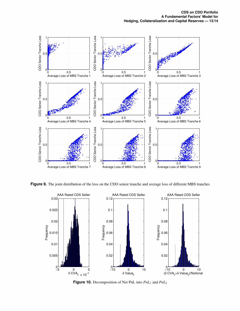
A firm faces two kinds of losses on the CDS contract: i) themark to market losses on the contract value and ii) mark tomarket of the CVA Denoting time by t, value of the contract

at t by Vt , collateral posted by counterparty at t by Ct , we canwrite the Profit and Loss equations:

PnL1 =Vt+1−Vt −Ct

PnL2 =CVAt −CVAt+1

Note that CVA is a loss by definition and hence PnL2is definedby subtracting the latest CVA value from the previous value.For the purpose of illustration, we do the capital reserve cal-culation only for the seller of the CDS contract for a horizonof a quarter. Note that the two losses described above are cor-related as both depend upon contract value. We already have2000 samples of Vt+1 ( using the LSM approach described inthe above section). For each V i

t+1 where i represents the ithpath we calculate the total loss PnLi = PnLi

1 +PnLi2 and get

the total loss distribution at t+1. In order to calculate PnLi2we

need to get the CVA values at t+1. We once again use LSMapproach to calculate CVA at each node n at t = 3 months.CVA at t = 3 months is the predicted value of the regressionbelow:

CVA(t) =α +β1Ht +β2H2t +β3H3

t + (25)

γ1rt + γ2r2t + γ3r3

t + (26)

θ1 logHt +θ2(logHt)2 +θ3Htrt (27)

For estimation of the regression coefficients we use the path-wise CVA values based upon the realized cash flows along aparticular path.

Capital Reserve is 1% percentile (i.e. 99% VaR) of the totalPnL distribution.The graphs below illustrates that with ourcollateral scheme the variation of the CVA loss distributionand the hence the CVA capital reserve requirement are stablefor various possible ratings of the CDS seller. This result isexpected as our collateral scheme requires low rated CDSsellers to post more collateral than is posted by high ratedCDS seller. Eventually the CDS buyer face the same CVAirrespective of the rating of the CDS seller. However if weconsider a fixed collateral posting (Figure 6), the variationin the CVA losses increases as the rating of the CDS sellerdepreciates. Hence the capital reserve requirements for theCDS buyer will increase.

It worth mentioning that the PnL distribution in the Figure 10looks same. However, they are similar but not the same.The graph below shows the 1% VaR of the PnL distributionand clarifies the presence of some variation amongst the PnLdistribution. In the Figure 6, The red vertical line represents99% VaR.

We illustrated the concept of capital reserve only for one prod-uct. However, in practice, we need to take into account thenet PnL of the firm taking into consideration all the posi-tions the firm is holding and carefully netting while modelingcorrelation between various positions.

CDS on CDO PortfolioA Fundamental Factors’ Model for

Hedging, Collateralization and Capital Reserves — 11/14

−5 0 5

x 10−3

0

0.02

0.04

δ CVAT

Fre

quen

cyAAA Rated CDS Seller

−5 0 5

x 10−3

0

0.02

0.04

δ CVAT

Fre

quen

cy

AA Rated CDS Seller

−5 0 5

x 10−3

0

0.02

0.04

δ CVAT

Fre

quen

cy

A Rated CDS Seller

−5 0 5

x 10−3

0

0.02

0.04

δ CVAT

Fre

quen

cy

BBB Rated CDS Seller

−5 0 5

x 10−3

0

0.02

0.04

δ CVAT

Fre

quen

cy

BB Rated CDS Seller

−5 0 5

x 10−3

0

0.02

0.04

δ CVAT

Fre

quen

cy

B Rated CDS Seller

Figure 6. Distribution of CVA PnL for Different SellerRatings with the Proposed Collateral Scheme

7. Conclusion

In this study, we revisited the series of events that leads tothe bailout of AIG. The AIG’s near-collapse is rooted with itshuge cumulated position in the CDS contracts on the supersenior tranches of CDOs, which were primarily backed bysubprime MBS. We implemented a macro-economical factormodel to simulate the cash flows of such CDS contract basedon HPI and interests rate. Schemes were proposed to hedgeCDS contact on MBS by ABX.HE indices, put options onmortgage market participants, and vanilla Eurodollar and HPIfutures. Simulations and hedging results are presented. Wecarried on to model the counterparty risk of this type of CDScontract and the effects of collateral schemes on the CVAvaluation. We demonstrated a framework to calculate the VaRon the CVA, and proposed a model of using the CVA VaR ascapital requirements for counterparty risks.

References

American International Group (2007). American internationalgroup, annual report 2008.

American International Group (2008). American internationalgroup, annual report 2008.

American International Group (2009). Collateral PostingsUnder AIGFP CDS.

Basel Committee (2010). Basel iii: International frameworkfor liquidity risk measurement, standards and monitoring.

Boyd, R. (2011). Fatal risk: a cautionary tale of AIG’scorporate suicide. John Wiley & Sons.

Congressional Oversight Panel (2010). June oversight report:

−0.2 −0.1 00

0.02

0.04

δ CVAT

Fre

quen

cy

AAA Rated CDS Seller

−0.2 −0.1 00

0.02

0.04

δ CVAT

Fre

quen

cy

AA Rated CDS Seller

−0.2 −0.1 00

0.02

0.04

δ CVAT

Fre

quen

cy

A Rated CDS Seller

−0.2 −0.1 00

0.02

0.04

δ CVAT

Fre

quen

cy

BBB Rated CDS Seller

−0.2 −0.1 00

0.02

0.04

δ CVAT

Fre

quen

cy

BB Rated CDS Seller

−0.2 −0.1 00

0.02

0.04

δ CVAT

Fre

quen

cy

B Rated CDS Seller

Figure 7. Distribution of CVA PnL for Different SellerRatings with the 75% Collateral Scheme

1 2 3 4 5 6−3.42

−3.4

−3.38

−3.36

−3.34

−3.32

−3.3

−3.28

−3.26

−3.24

−3.22x 10

−3

99 p

erce

ntile

CV

A L

oss

VA

R

Seller Rating

Figure 8. 99% VaR of CVA with Different Sellers Rating

The aig rescue, its impact on markets, and the government’sexit strategy.

Dolan, J. (2011). Home price futures blog.

Downing, C., Stanton, R., and Wallace, N. (2005). An empir-ical test of a two-factor mortgage valuation model: Howmuch do house prices matter? Real Estate Economics,33(4):681–710.

Hull, J. and White, A. (1993). One-factor interest-rate mod-els and the valuation of interest-rate derivative securities.Journal of financial and quantitative analysis, 28(2).

Longstaff, F. A. and Schwartz, E. S. (2001). Valuing americanoptions by simulation: A simple least-squares approach.Review of Financial studies, 14(1):113–147.

CDS on CDO PortfolioA Fundamental Factors’ Model for

Hedging, Collateralization and Capital Reserves — 12/14

Lucas, D., Goodman, L., and Fabozzi, F. (2007). Collateral-ized debt obligations and credit risk transfer.

Schwartz, E. S. and Torous, W. N. (1989). Prepayment andthe valuation of mortgage-backed securities. The Journalof Finance, 44(2):375–392.

Sjostrom Jr, W. K. (2009). Aig bailout, the. Wash. & Lee L.Rev., 66:943.

S&P Indices (2011). S&p/case-shiller home price indicesfrequently asked questions.

Stanton, R., Walden, J., and Wallace, N. (2014). The industrialorganization of the u.s. residential mortgage market. AnnualReview of Financial Economics, 6(1).

Stanton, R. and Wallace, N. (2011). The bear’s lair: Indexcredit default swaps and the subprime mortgage crisis. Re-view of Financial Studies, 24(10):3250–3280.

TPM (2009). The rise and fall of aig’s financial products unit.

Appendix

CDS on CDO PortfolioA Fundamental Factors’ Model for

Hedging, Collateralization and Capital Reserves — 13/14

0 0.5 10

0.5

1C

DO

Senio

r T

ranche L

oss

Average Loss of MBS Tranche 10 0.5 1

0

0.5

1

CD

O S

enio

r T

ranche L

oss

Average Loss of MBS Tranche 20 0.5 1

0

0.5

1

CD

O S

enio

r T

ranche L

oss

Average Loss of MBS Tranche 3

0 0.5 10

0.5

1

CD

O S

enio

r T

ranche L

oss

Average Loss of MBS Tranche 40 0.5 1

0

0.5

1

CD

O S

enio

r T

ranche L

oss

Average Loss of MBS Tranche 50 0.5 1

0

0.5

1

CD

O S

enio

r T

ranche L

oss

Average Loss of MBS Tranche 6

0 0.5 10

0.5

1

CD

O S

enio

r T

ranche L

oss

Average Loss of MBS Tranche 70 0.5 1

0

0.5

1

CD

O S

enio

r T

ranche L

oss

Average Loss of MBS Tranche 80 0.5 1

0

0.5

1

CD

O S

enio

r T

ranche L

oss

Average Loss of MBS Tranche 9

Figure 9. The joint distribution of the loss on the CDO senior tranche and average loss of different MBS tranches

−5 0 5

x 10−3

0

0.005

0.01

0.015

0.02

0.025

0.03

δ CVAT

Fre

quency

AAA Rated CDS Seller

−10 0 100

0.02

0.04

0.06

0.08

0.1

0.12

δ ValueT

Fre

quency

AAA Rated CDS Seller

−10 0 100

0.02

0.04

0.06

0.08

0.1

0.12

(δ CVAT+δ Value

T)/Notional

Fre

quency

AAA Rated CDS Seller

Figure 10. Decomposition of Net PnL into PnL1 and PnL2

CDS on CDO PortfolioA Fundamental Factors’ Model for

Hedging, Collateralization and Capital Reserves — 14/14

Cash Flow Distributed From The Top

Default / Write-off Starts From the Bottum

CDO Cash FlowTranch Cash Flow ModelingLoan Pool Cash Flow Modeling

M10

M9

M8

A2

A1

x Coupon

x Prepayment Probability

Amortization Math

x Default Probability

After Default Adjustment

Previous Month Balance

After Amortization

End of Month Balance

Prepayments

Principal Payments

Interest Payments

CDO Cashflow

CDO Default

Default CF

Figure 11. Schematic Design of MBS Cash Flow Modeling

(Index Member) (Index Member) (Index Member)

1

2

3

4

5

6

7

8

9

λ(1) (t; ε(1) ) λ(2) (t; ε(2) ) λ(3) (t; ε(2) ) λ(4) (t; ε(4) ) λ(100) (t; ε(100) )

10

CDO Pool (20 traches for each seniority) Default Amount

ABX Index

Cash Flows

ABX Index 2

ABX Index 6

JIHBA

Default Loss Default Loss Default Loss Default Loss Default Loss

CDO Tranches

CDS Proection

(PAUG)

......

......

......

Figure 12. Schematic Design of CDOs, ABX Cash Flows Modeling