107
CE 8214: Transportation Economics: Introduction David Levinson
| Date post: | 19-Dec-2015 |
| Category: |
Documents |
| View: | 222 times |
| Download: | 1 times |

CE 8214: Transportation Economics: Introduction
David Levinson

Introductions
• Who are you? • State your name, major/profession,
degree goal, research interest

Syllabus
• Handouts• Textbook

Paper reviews
• handouts

The game
• 1. An indefinitely repeated round-robin
• 2. A payoff matrix• 3. Odds & Evens• 4. The strategy (write it down, keep it
secret for now)• 5. Scorekeeping (record your score …
honor system)• 6. The prize: The awe of your peers

The Payoff Matrix
Player BOdd
Player BEven
Player AOdd
[3, 3] [0, 5]
Player AEven
[5, 0] [1, 1]
[Payoff A, Payoff B]

Roundrobin Schedules
• How many students …

11 Players
11. Rou nd ro bin schedul e fo r 11 teams. A B C D E Bye 6 - 7 5- 8 4- 9 3- 10 2- 11 1 7 - 8 6- 9 5- 10 4- 11 3- 1 2 8 - 9 7- 10 6- 11 5- 1 4- 2 3 9 - 10 8- 11 7- 1 6- 2 5- 3 410- 11 9- 1 8- 2 7- 3 6- 4 511- 1 10- 2 9- 3 8- 4 7- 5 6 1 - 2 11- 3 10- 4 9- 5 8- 6 7 2 - 3 1- 4 11- 5 10- 6 9- 7 8 3 - 4 2- 5 1- 6 11- 7 10- 8 9 4 - 5 3- 6 2- 7 1- 8 11- 9 10 5 - 6 4- 7 3- 8 2- 9 1- 10 11

12 Players
12. Round ro bin schedul e fo r 12 te ams. A B C D E B ye 7 - 8 6- 9 5- 10 4- 11 3- 12 1 2 8 - 9 7- 10 6- 11 5- 12 3- 1 2 4 9 - 10 8- 11 7- 12 5- 1 4- 2 3 610- 11 9- 12 7- 1 6- 2 5- 3 4 811- 12 9- 1 8- 2 7- 3 6- 4 5 1011- 1 10- 2 9- 3 8- 4 7- 5 6 1212- 2 11- 3 10- 4 9- 5 8- 6 1 7 1 - 2 12- 4 11- 5 10- 6 9- 7 3 8 2 - 3 1- 4 12- 6 11- 7 10- 8 5 9 3 - 4 2- 5 1- 6 12- 8 11- 9 7 10 4 - 5 3- 6 2- 7 1- 8 12- 10 9 11 5 - 6 4- 7 3- 8 2- 9 1- 10 11 12 3 - 10 2- 11 1- 12 4 5 6 7 8 9 6 - 7 5- 8 4- 9 1 2 3 10 11 12

13 Players
13. Rou nd ro bin schedul e fo r 13 teams. A B C D E F Bye 7 - 8 6- 9 5- 10 4- 11 3- 12 2- 13 1 8 - 9 7- 10 6- 11 5- 12 4- 13 3- 1 2 9 - 10 8- 11 7- 12 6- 13 5- 1 4- 2 310- 11 9- 12 8- 13 7- 1 6- 2 5- 3 411- 12 10- 13 9- 1 8- 2 7- 3 6- 4 512- 13 11- 1 10- 2 9- 3 8- 4 7- 5 613- 1 12- 2 11- 3 10- 4 9- 5 8- 6 7 1 - 2 13- 3 12- 4 11- 5 10- 6 9- 7 8 2 - 3 1- 4 13- 5 12- 6 11- 7 10- 8 9 3 - 4 2- 5 1- 6 13- 7 12- 8 11- 9 10 4 - 5 3- 6 2- 7 1- 8 13- 9 12- 10 11 5 - 6 4- 7 3- 8 2- 9 1- 10 13- 11 12 6 - 7 5- 8 4- 9 3- 10 2- 11 1- 12 13

14 Players 14. Round ro bin schedul e fo r 14 te ams. A B C D E F B ye 8 - 9 7- 10 6- 11 5- 12 4- 13 3- 14 1 2 9 - 10 8- 11 7- 12 6- 13 5- 14 3- 1 2 410- 11 9- 12 8- 13 7- 14 5- 1 4- 2 3 611- 12 10- 13 9- 14 7- 1 6- 2 5- 3 4 812- 13 11- 14 9- 1 8- 2 7- 3 6- 4 5 1013- 14 11- 1 10- 2 9- 3 8- 4 7- 5 6 1213- 1 12- 2 11- 3 10- 4 9- 5 8- 6 7 1414- 2 13- 3 12- 4 11- 5 10- 6 9- 7 1 8 1 - 2 14- 4 13- 5 12- 6 11- 7 10- 8 3 9 2 - 3 1- 4 14- 6 13- 7 12- 8 11- 9 5 10 3 - 4 2- 5 1- 6 14- 8 13- 9 12- 10 7 11 4 - 5 3- 6 2- 7 1- 8 14- 10 13- 11 9 12 5 - 6 4- 7 3- 8 2- 9 1- 10 14- 12 11 13 6 - 7 5- 8 4- 9 3- 10 2- 11 1- 12 13 14 4 - 11 3- 12 2- 13 1- 14 5 6 7 8 9 10 7 - 8 6- 9 5- 10 1 2 3 4 11 12 13 14 You may wish to swap ro unds 2 and 13,in order to dist r ibut e th e byes mor e evenly.

15 Players
15. Round ro bin schedul e fo r 15 te ams. A B C D E F G Bye 8 - 9 7- 10 6- 11 5- 12 4- 13 3- 14 2- 15 1 9 - 10 8- 11 7- 12 6- 13 5- 14 4- 15 3- 1 210- 11 9- 12 8- 13 7- 14 6- 15 5- 1 4- 2 311- 12 10- 13 9- 14 8- 15 7- 1 6- 2 5- 3 412- 13 11- 14 10- 15 9- 1 8- 2 7- 3 6- 4 513- 14 12- 15 11- 1 10- 2 9- 3 8- 4 7- 5 614- 15 13- 1 12- 2 11- 3 10- 4 9- 5 8- 6 715- 1 14- 2 13- 3 12- 4 11- 5 10- 6 9- 7 8 1 - 2 15- 3 14- 4 13- 5 12- 6 11- 7 10- 8 9 2 - 3 1- 4 15- 5 14- 6 13- 7 12- 8 11- 9 10 3 - 4 2- 5 1- 6 15- 7 14- 8 13- 9 12- 10 11 4 - 5 3- 6 2- 7 1- 8 15- 9 14- 10 13- 11 12 5 - 6 4- 7 3- 8 2- 9 1- 10 15- 11 14- 12 13 6 - 7 5- 8 4- 9 3- 10 2- 11 1- 12 15- 13 14 7 - 8 6- 9 5- 10 4- 11 3- 12 2- 13 1- 14 15

16 Players 16. Round ro bin schedul e fo r 16 te ams. A B C D E F G B ye 9 - 10 8- 11 7- 12 6- 13 5- 14 4- 15 3- 16 1 210- 11 9- 12 8- 13 7- 14 6- 15 5- 16 3- 1 2 411- 12 10- 13 9- 14 8- 15 7- 16 5- 1 4- 2 3 612- 13 11- 14 10- 15 9- 16 7- 1 6- 2 5- 3 4 813- 14 12- 15 11- 16 9- 1 8- 2 7- 3 6- 4 5 1014- 15 13- 16 11- 1 10- 2 9- 3 8- 4 7- 5 6 1215- 16 13- 1 12- 2 11- 3 10- 4 9- 5 8- 6 7 1415- 1 14- 2 13- 3 12- 4 11- 5 10- 6 9- 7 8 1616- 2 15- 3 14- 4 13- 5 12- 6 11- 7 10- 8 1 9 1 - 2 16- 4 15- 5 14- 6 13- 7 12- 8 11- 9 3 10 2 - 3 1- 4 16- 6 15- 7 14- 8 13- 9 12- 10 5 11 3 - 4 2- 5 1- 6 16- 8 15- 9 14- 10 13- 11 7 12 4 - 5 3- 6 2- 7 1- 8 16- 10 15- 11 14- 12 9 13 5 - 6 4- 7 3- 8 2- 9 1- 10 16- 12 15- 13 11 14 6 - 7 5- 8 4- 9 3- 10 2- 11 1- 12 16- 14 13 15 7 - 8 6- 9 5- 10 4- 11 3- 12 2- 13 1- 14 15 16 4 - 13 3- 14 2- 15 1- 16 5 6 7 8 9 10 11 12 8 - 9 7- 10 6- 11 5- 12 1 2 3 413 14 15 16

17 Players 17. Round ro bin schedul e fo r 17 te ams. A B C D E F G H Bye 9 - 10 8- 11 7- 12 6- 13 5- 14 4- 15 3- 16 2- 17 110- 11 9- 12 8- 13 7- 14 6- 15 5- 16 4- 17 3- 1 211- 12 10- 13 9- 14 8- 15 7- 16 6- 17 5- 1 4- 2 312- 13 11- 14 10- 15 9- 16 8- 17 7- 1 6- 2 5- 3 413- 14 12- 15 11- 16 10- 17 9- 1 8- 2 7- 3 6- 4 514- 15 13- 16 12- 17 11- 1 10- 2 9- 3 8- 4 7- 5 615- 16 14- 17 13- 1 12- 2 11- 3 10- 4 9- 5 8- 6 716- 17 15- 1 14- 2 13- 3 12- 4 11- 5 10- 6 9- 7 817- 1 16- 2 15- 3 14- 4 13- 5 12- 6 11- 7 10- 8 9 1 - 2 17- 3 16- 4 15- 5 14- 6 13- 7 12- 8 11- 9 10 2 - 3 1- 4 17- 5 16- 6 15- 7 14- 8 13- 9 12- 10 11 3 - 4 2- 5 1- 6 17- 7 16- 8 15- 9 14- 10 13- 11 12 4 - 5 3- 6 2- 7 1- 8 17- 9 16- 10 15- 11 14- 12 13 5 - 6 4- 7 3- 8 2- 9 1- 10 17- 11 16- 12 15- 13 14 6 - 7 5- 8 4- 9 3- 10 2- 11 1- 12 17- 13 16- 14 15 7 - 8 6- 9 5- 10 4- 11 3- 12 2- 13 1- 14 17- 15 16 8 - 9 7- 10 6- 11 5- 12 4- 13 3- 14 2- 15 1- 16 17

Discussion
• What does this all mean?• System Rational vs. User Rational• Tit for Tat vs. Myopic Selfishness

Next Time
• Email me your reviews by Tuesday 5:30 pm.
• Talk with me if you have problem with your assigned Discussion Paper.
• Discuss Game Theory

Game Theory
David Levinson

Overview
• Game theory is concerned with general analysis of strategic interaction of economic agents whose decisions affect each other.

Problems that can be Analyzed with Game
Theory• Congestion• Financing• Merging• Bus vs. Car• [] … who are the agents?

Dominant Strategy• A Dominant Strategy is one in which one choice clearly dominates
all others while a non-dominant strategy is one that has superior strategies.
• DEFINITION Dominant Strategy: Let an individual player in a game evaluate separately each of the strategy combinations he may face, and, for each combination, choose from his own strategies the one that gives the best payoff. If the same strategy is chosen for each of the different combinations of strategies the player might face, that strategy is called a "dominant strategy" for that player in that game.
• DEFINITION Dominant Strategy Equilibrium: If, in a game, each player has a dominant strategy, and each player plays the dominant strategy, then that combination of (dominant) strategies and the corresponding payoffs are said to constitute the dominant strategy equilibrium for that game.

Nash Equilibrium
• Nash Equilibrium (NE): a pair of strategies is defined as a NE if A's choice is optimal given B's and B's choice is optimal given A's choice.
• A NE can be interpreted as a pair of expectations about each person's choice such that once one person makes their choice neither individual wants to change their behavior. For example,
• DEFINITION: Nash Equilibrium If there is a set of strategies with the property that no player can benefit by changing her strategy while the other players keep their strategies unchanged, then that set of strategies and the corresponding payoffs constitute the Nash Equilibrium.
• NOTE: any dominant strategy equilibrium is also a Nash Equilibrium

A Nash Equilibrium
B
i j
A i [3,3]* [2,2]
j [2,2] [1,1]

Representation
• Payoffs for player A are represented is the first number in a cell, the payoffs for player B are given as the second number in that cell. Thus strategy pair [i,i] implies a payoff of 3 for player A and also a payoff of 3 for player B. The NE is asterisked in the above illustrations. This represents a situation in which each firm or person is making an optimal choice given the other firm or persons choice. Here both A and B clearly prefer choice i to choice j. Thus [i,i] is a NE.

Prisoner’s Dilemma
• Last week in class, we played both a finite one-time game and an indefinitely repeated game. The game was formulated as what is referred to as a ‘prisoner’s dilemma’.
• The term prisoner’s dilemma comes from the situation where two partners in crime are both arrested and interviewed separately . – If they both ‘hang tough’, they get light sentences for lack
of evidence (say 1 year each). – If they both crumble in interrogation and confess, they
both split the time for the crime (say 10 years). – But if one confesses and the other doesn’t, the one who
confesses turns state’s evidence (and gets parole) and helps convict the other (who does 20 years time in prison)

P.D. Dominant Strategy
• In the one-time or finitely repeated Prisoners' Dilemma game, to confess (toll, defect, evens) is a dominant strategy, and when both prisoners confess (states toll, defect, evens), that is a dominant strategy equilibrium.

Example: Tolling at a Frontier
• Two states (Delaware and New Jersey) are separated by a body of water. They are connected by a bridge over that body. How should they finance that bridge and the rest of their roads?
• Should they toll or tax?
• Let rI and rJ are tolls of the two jurisdictions. Demand is a negative exponential function.
• (Objective, minimize payoff)

ObjectivesObjective FunctionLocal welfare
max
rI
WL
= Ui j
+ 2 * Ri j
− 2 * CN i j
− 2 * CV i j
Component EquationsFlow
f
b
= ω e
α rI
+ rJ
( )
(1)
Consumer'ssurplus
Uij
= ω e
α p( )
∂ p
rτ
+ rJ
∞
∫
= −
ω e
α r
I
+ r
J( )
α
(2)
Networ k us e costC
Nij
=
φ
ψ
ω e
α rI
+ rJ
( )
(3)
Collection costC
Vij
= θ ω e
α rI
+ rJ
( ) (4)
RevenueR
ij
= rI
ω e
α rI
+ rJ
( )
(5)

Payoffs
• The table is read like this: Each jurisdiction chooses one of the two strategies (Toll or Tax). In effect, Jurisdiction 1 (Delaware) chooses a row and jurisdiction 2 (New Jersey) chooses a column. The two numbers in each cell tell the outcomes for the two states when the corresponding pair of strategies is chosen. The number to the left of the comma tells the payoff to the jurisdiction who chooses the rows (Delaware) while the number to the right of the column tells the payoff to the state who chooses the columns (New Jersey). Thus (reading down the first column) if they both toll, each gets $1153/hour in welfare , but if New Jersey Tolls and Delaware Taxes, New Jersey gets $2322 and Delaware only $883.
JJ New JerseyToll Tax
JI Delaware Toll [1153, 1153]* [2322, 883]Tax [883, 2322] [1777, 1777]

Solution
• So: how to solve this game? What strategies are "rational" if both states want to maximize welfare? New Jersey might reason as follows: "Two things can happen: Delaware can toll or Delaware can keep tax. Suppose Delaware tolls. Then I get only $883 if I don't toll, $1153 years if I do, so in that case it's best to toll. On the other hand, if Delaware taxes and I toll, I get $2322, and if I tax we both get $1777. Either way, it's best if I toll. Therefore, I'll toll."
• But Delaware reasons similarly. Thus they both toll, and lost $624/hour. Yet, if they had acted "irrationally," and taxed, they each could have gotten $1777/hour.

Coordination Game
• In Britain, Japan, Australia, and some other island nations people drive on the left side of the road; in the US and the European continent they drive on the right. But everywhere, everyone drives on the same side as everywhere else, even if that side changes from place to place.
• How is this arrangement achieved?• There are two strategies: drive on the left side and
drive on the right side. There are two possible outcomes: the two cars pass one another without incident or they crash. We arbitrarily assign a value of one each to passing without problems and of -10 each to a crash. Here is the payoff table:

Coordination Game Payoff Table
MercedesL R
Buick L [1,1] [-10,-10]R [-10,-10] [1,1]

Coordination Discussion
• (Objective: Maximize payoff) • Verify that LL and RR are both Nash equilibria. • But, if we do not know which side to choose,
there is some danger that we will choose LR or RL at random and crash. How can we know which side to choose? The answer is, of course, that for this coordination game we rely on social convention. Conversely, we know that in this game, social convention is very powerful and persistent, and no less so in the country where the solution is LL than in the country where it is RR

Issues in Game Theory
• What is “rationality” ?• What happens when the rational strategy depends
on strategies of others?• What happens if information is incomplete?• What happens if there is uncertainty or risk?• Under what circumstances is cooperation better
than selfishness? Under what circumstances is cooperation selfish?
• How do continuing interactions differ from one-time events?
• Can morality be derived from rational selfishness?• How does reality compare with game theory?

Discussion
• How does an infinitely or indefinitely repeated Prisoner’s Dilemma game differ from a finitely repeated or one-time game?
• Why?

Problem
• Two airlines (United, American) each offer 1 flight from New York to Los Angeles. Price = $/pax, Payoff = $/flight. Each plane carries 500 passengers, fixed cost is $50000 per flight, total demand at $200 is 500 passengers. At $400, total demand is 250 passengers. Passengers choose cheapest flight. Payoff = Revenue - Cost
• Work in pairs (4 minutes): • Formulate the Payoff Matrix for the Game

Solution
AmericanPrice=$200 Price=$400
United Price=$200 [0,0 ] [50000, -50000]Price=$400 [-50000, 50000 ] [0,0]

Zero-Sum
• DEFINITION: Zero-Sum game If we add up the wins and losses in a game, treating losses as negatives, and we find that the sum is zero for each set of strategies chosen, then the game is a "zero-sum game."
• 2. What is equilibrium ?

• [$200,$200]
• SOLUTION: Maximin criterion For a two-person, zero sum game it is rational for each player to choose the strategy that maximizes the minimum payoff, and the pair of strategies and payoffs such that each player maximizes her minimum payoff is the "solution to the game."
• 3. What happens if there is a third price $300, for which demand is 375 passengers.

3 Possible Strategies
• At [300,300] Each airline gets 375/2 share = 187.5 pax * $300 = $56,250, cost remains $50,000
• At [300, 400], 300 airline gets 375*300 = 112,500 - 50000
AmericanPrice=$200 Price=$300 Price=$400
United Price=$200 [0,0] [50000, -50000] [50000, -50000 ]Price=$300 [-50000, 50000 ] [6250, 6250] [62500, - 50000]Price=$400 [-50000, 50000] [-50000, 62500] [0,0]

Mixed Strategies?
• What is the equilibrium in a non-cooperative, 1 shot game?
• [$200,$200].• What is equilibrium in a repeated game?• Note: No longer zero sum.• DEFINITION Mixed strategy If a
player in a game chooses among two or more strategies at random according to specific probabilities, this choice is called a "mixed strategy."

Microfoundations of Congestion and Pricing
David Levinson

Objective of Research
• To build simplest model that explains congestion phenomenon and shows implications of congestion pricing.
• Uses game theory to illustrate ideas, informed by structure of congestion problems – simultaneous arrival;– arrival rate > service flow; – first-in, first-out queueing, – delay cost, – schedule delay cost

Game Theory Assumptions
• Actors are instrumentally rational – (actors express preferences and act to satisfy them)
• Common knowledge of rationality – (each actor knows each other actor is instrumentally
rational, and so on)
• Consistent alignment of beliefs – (each actor, given same information and
circumstances, would make same choice)
• Actors have perfect knowledge

Application of Games in Transportation
• Fare evasion and compliance (Jankowski 1990)
• Truck weight limits (Hildebrand 1990)• Merging behavior (Kita et al. 2001)• Highway finance choices (Levinson
1999, 2000)• Airports and Aviation (Hansen 1988,
2001)• …

Two-Player Congestion Game
• Penalty for Early Arrival (E), Late Arrival (L), Delayed (D)
• Each vehicle has option of departing (from home) early (e), departing on-time (o), or departing (l)
• If two vehicles depart from home at the same time, they will arrive at the queue at the same time and there will be congestion. One vehicle will depart the queue (arrive at work) in that time slot, one vehicle will depart the queue in the next time slot.

Congesting Strategies
If both individuals depart early (a strategy pair we denote as ee), one will arrive early and one will be delayed but arrive on-time. We can say that each individual has a 50% chance of being early or being delayed.
If both individuals depart on-time (strategy oe), one will arrive on-time and one will be delayed and arrive late. Each individual has a 50% chance of being delayed and being late.
• If both individuals depart late (strategy ll), one will arrive late and one will be delayed and arrive very late. Each individual has a 50% change of being delayed and being very late.

Payoff Matrix
Vehicle 2Early On-time Late
Early [0.5*(E+D),0.5*(E+D)]
[E,0]
[E,L]
Vehicle 1 On-time [0,E]
[0.5*(L+D),0.5*(L+D)]
[0,L]
Late [L,E]
[L,0]
[L+0.5*(L+D),L+0.5*(L+D)]
Note: [Payout for Vehicle 1, Payout for Vehicle 2]
Objective to Minimize Own Payout, S.t. others doing same

Example 1: (1,0,1)
E, D, L Vehicle 21, 0, 1 Early On-time Late
Early [0.5,0.5] [1,0] [1,1]Vehicle 1 On-time [0,1] [0.5, 0.5] * [0,1]
Late [1,1] [1,0] [1.5, 1.5]
Note: * Indicates Nash Equilibrium
Italics indicates social welfare maximizing solution

Example 2: (3,1,4)
E, D, L Vehicle 23, 1, 4 Early On-time Late
Early [2,2] [3,0] [3,4]Vehicle 1 On-time [0,3] [2.5, 2.5] * [0,4]
Late [4,3] [4,0] [6.5, 6.5]
Note: * Indicates Nash Equilibrium
Italics indicates social welfare maximizing solution

Payoff matrix with congestion pricing
Vehicle 2Early On-time Late
Early [0.5*(E+D)+τe,0.5*(E+ ) D + τe]
[ ,E0]
[ ,E]L
Vehicl 1e On-time [0,]E
[0.5* ( +L D)+τo,0.5*(L+ ) D + τo]
[0,]L
Late [ ,L]E
[ ,L0]
[L+0.5*(L+ )+D τl,+0.5*L ( +L D) + τl]

What are the proper prices?
• Normally use marginal cost pricing– MC = ∂ TC/∂Q
• But Total Costs (TC) are discrete, so we use incremental cost pricing – IC = TC/Q
• Total Costs include both delay costs as well as schedule delay costs.– τo= τl =0.5*(L+D)– τe = MAX(0.5*(D-E),0)

Subtleties
• Vehicles may affect other vehicles by causing them to change behavior.
• Total costs do not include these “pecuniary” externalities such as displacement in time, just what the cost would be for that choice, given the other person is there, compared with the cost for that choice if one player were not there.
• You can’t blame departing early on the other player.

Example 1 (1,0,1) with congestion prices
E, D, L Vehicle 21, 0, 1 Early On-time Late
Early [0.5,0.5] [1,0]* [1,1]Vehicle 1 On-time [0,1]* [1,1]* [0,1]*
Late [1,1] [1,0]* [2,2]

Example 2 (3,1,4) with congestion prices
E, D, L Vehicle 23,1,4 Early On-time Late
Early [2.5,2.5] [3,0]* [3,4]Vehicle 1 On-time [0,3]* [5,5] [0,4]
Late [4,3] [4,0] [9,9]

Two-Player Game Results
E,D,LNumber of Nash
Equilibria (Unpriced)Solutions(Unpriced)
TotalCost
MinimumTotal Cost
Number of NashEquilibria (Priced)
Solutions(Priced)
0,0,0 9 all 0 0 9 all
0,1,06 eo, el, oe, ol,
le, lo0 0 6 eo, el, oe, ol,
le, lo0,0,1 3 ee, eo, oe 0 0 3 ee, eo, oe0,1,1 2 oe, eo 0 0 2 oe, eo1,0,0 4 oo, ol, lo, ll 0 0 4 oo, ol, lo, ll1,1,0 2 ol, lo 0 0 2 ol, lo
1,0,11 oo 1 1 5 eo, oe, oo,
ol, lo
1,1,15 eo, oe, oo, ol,
lo1 or 2 1 4 eo, oe, ol, lo
3,1,4 1 oo 5 3 2 oe, eo4,0,3 1 oo 3 3 3 oo, ol, lo4,1,3 1 oo 4 3 2 ol, lo3,0,4 1 oo 4 3 2 eo, oe

Three-Player Congestion Pricing Game
• The model can be extended. With more players, we need to add one departure from home (arrival at the back of the queue) time period, and two arrival at work (departure from the front of the queue) time periods.

Delay
• Expected delay• Cost of delay
• where:• D = delay penalty
• Qt = standing queue at time t
• At = arrivals at time t.
€
ε dt( ) = Qt + 0.5At( )
€
C dt( ) = Qt + 0.5At( )D

Schedule Delay
• Schedule delay is the deviation from the time which a vehicle departs the queue and the desired, or on-time period.
• Where:• dt = delay• ta = time of arrival at back of queue• to = desired time of departure from front of
queue (time to be on-time)• The cost of schedule delay is thus
€
Si = ta + dt − to
€
C Si( ) = E * Si , if Si < 0
= L * Si , if Si > 0

Probabilistics
• We only know the delay probabilistically, so schedule delay is also probabilistic
• Where:
• P() = probability function for traveler i, summarized in Table 9.
• t = penalty function = (2E, E, 0, L, 2L, 3L)• are the periods of departure
from the queue (very early, early, on-time, late, really late, super late).
€
E Si( ) = PtΠtt
∑ = P v ( ) * 2E + P e ( ) * E + P l ( ) * L + P r ( ) * 2L + P s ( ) * 3L
€
1 = Pt =t
∑ P v ( ) + P e ( ) + P o ( ) + P l ( ) + P r ( ) + P s ( )
€
v ,e ,o ,l ,r ,s

Nomenclature
• V - Very Early• E - Early• O - On-time• L - Late• R - Really Late• S - Super Late

Three-Player Game
Arrival and DeparturePatterns
ArrivalPattern
Frequency(/64)
DeparturePatterns
Frequency(/64)
vvv 1 veo 16vve 3vvo 3veo 6vee 3vvl 3 vel 9vel 6voo 3 vol 9vol 6vll 3 vlr 3eee 1 eol 16eeo 3eel 3eoo 3eol 6ell 3 elr 3
ooo 1 olr 7ool 3oll 3lll 1 lrs 1

Departure Probability Given Arrival Strategies
[v,_,_]
v v v v e e e o o lPlayer BPlayer C v e o l e o l o l l
Departure Probability
Player A v
€
P v ( ) 0.33 0.5 0.5 0.5 1 1 1 1 1 1
€
P e ( ) 0.33 0.5 0.5 0.5 0 0 0 0 0 0
€
P o ( ) 0.33 0 0 0 0 0 0 0 0 0
€
P l ( ) 0 0 0 0 0 0 0 0 0 0
€
P r ( ) 0 0 0 0 0 0 0 0 0 0
€
P s ( ) 0 0 0 0 0 0 0 0 0 0

Three-Player Game Results
E,D,L
Number ofNash
Equilibria(Unpriced) Solutions (Unpriced)
Numberof Nash
Equilibria(Priced) Solutions (Priced)
LowestTotal Cost
0,0,0 64 all 64 all 00,1,0 24 veo …, vel …, vol …, eol … , 24 veo …, vel …, vol …, eol … , 00,0,1 13 vvv, vvo …, vee … , veo, … 13 vvv, vvo …, vee … , veo, … 00,1,1 6 veo, … 6 veo, … 01,0,0 8 ooo,lll,oll, …, ool … 8 ooo,lll,llo, …, ool … 01,1,0 7 ooo, ool …, oll, … 3 llo, … 11,0,1 5 ooo, eee, … eeo, … 4 eee, eeo, … 21,1,1 9 eol, … , eoo, … 6 eol, … 23,1,4 1 eee 3 eoo, … 74,0,3 2 ooo, eee 4 eee, eoo 74,1,3 4 ooo, eoo, ... 9 eol, …, eoo 73,0,4 1 eee 1 eee 7

Conclusions
• Presented a simple (the simplest?) model of congestion and pricing.
• A new way of viewing congestion and pricing in the context of game theory.
• Illustrates the effectiveness of moving equilibria from individually to socially optimal solutions.
• Extensions: empirical estimates of E, D, L; risk; uncertainty and stochastic behavior; simulations with more players.

Break

On Whom The Toll Falls: A Model of Network Financing
by David Levinson
Man in Bowler Hat:
To Boost The British Economy, I’d Tax All Foreigners Living Abroad
-- Chapman et al. (1989)

Outline• Research Questions, Motivation, &
Hypotheses• Historical Background• Actors & Actions • Free Riders & Cross Subsidies• Analytical Model• Empirical Values• Model Evaluation• Conclusions

Research Questions• How and why has the preferred
method of highway financing changed over time between taxes and tolls?
• Who wins and who loses under various revenue mechanisms?
• How does the spatial distribution of winners and losers affect the choice?

Motivation• New Capacity Desired• New Concerns: Social Costs• New Fleet: EVs• New Networks: ITS • New Toll Technology: ETC• New Owners: Privatization• New Rules: ISTEA 2• New Priorities:
– Capital -> Operating

HypothesisHypothesis: Jurisdiction Size & Collection Costs
Influence Revenue Choice.• Cross-subsidies from non-locals to locals will
be more politically palatable than vice versa.• Small jurisdictions can affect cross-subsidies
more easily with tolls than large jurisdictions.• New technologies lower toll collection costs.

Actors and Actions• Jurisidiction/ Road Authority:
– Operates Local Roads– Serves Local & Non-Local Travelers – Sets Revenue Mechanism & Rate – Has Poll Tax Authority– Objective: Local “Welfare” Maximization (Sum of
Profit to Road and Consumers’ Surplus of Residents)
• Travelers– Travel on Local & Non-Local Roads– Collectively “Own” Jurisdiction of Residence

Revenue Instrument
Instrument Example Where
Collected
System
Access Tax
Poll Tax home
jurisdiction
Use-Based
Tax
Odometer Tax home
jurisdiction,
Cordon Toll Toll to Cross
Cordon
jurisdiction of
use
Perfect Toll Toll on Every
Segment
jurisdiction of
use

Why No Gas Tax ?
The Gas Tax is bounded by two cases: • Odometer Tax (where all gas
purchased in the home jurisdiction) and
• Perfect Toll (where all gas purchased in the jurisdiction of travel).
What is proper behavioral assumption about location of purchase?

Long Road &
Trip Classes
- ∞
a b
- ∞ ∞J0
a b
- ∞ ∞J0
a b
- ∞ ∞J0
a b
- ∞ ∞J0
xy
Class G0+ Trips
yx ∞
Class G-0 Trips
x y
x- ∞ y ∞
Class G-+ Trips
Class G00 Trips
Long Road
S- S+
a bJ0 J+1 J+2
-∞ ∞
s.t. y > x for all trips

Free RidersClass of Rider Share (S) of Full
Cost Paid
Perfect Free Riders 0%
Imperfect Free Riders or
Easy Riders
0% < S < 100%
Fair Riders 100%
Overburdened or Hard
Riders
100% < S

Cross Subsidy by Instrument & Class
User Group
OriginDestination
Instrument
LocalLocal
(G00)
LocalNon-Local
(G0+)
Non-LocalLocal
(G-0)
Non-LocalNon-Local(Through)(G-+)
SystemAccessTax
Hard Hard -residentsFree - non-residents
Hard -residentsFree - non-residents
Free
Use-Based(Odometer)Tax
Hard Hard -residentsFree - non-residents
Hard -residentsFree - non-residents
Free
Cordon Toll Free Hard/Fair/Easy
Hard/Fair/Easy
Hard
Perfect Toll Fair Fair Fair Fair
Assumes Total Cost=Total Revenue; “Fair” is proportional to distance traveled

Model Parameters• Demand:
– Distance, – Price of Trip, – Fixed User Cost.
• Network Cost: – Fixed Network Costs, – Variable Network Costs, – Fixed Collection Costs,– Variable Collection Costs.
• Network Revenue:– Rate of Toll, Tax,– Basis.
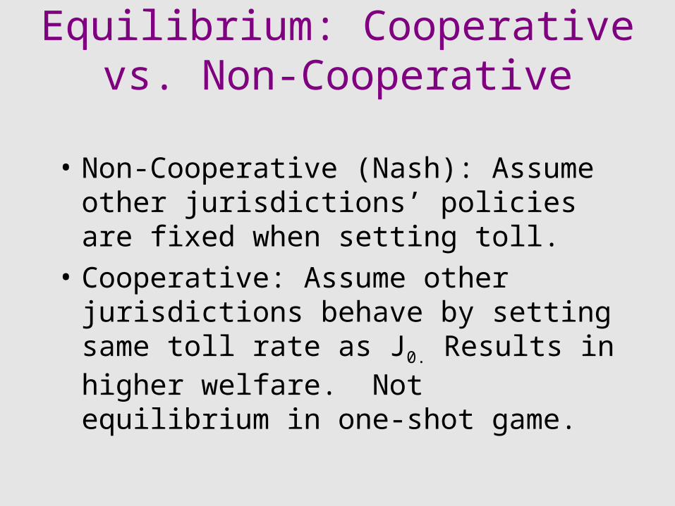
Equilibrium: Cooperative vs. Non-Cooperative
• Non-Cooperative (Nash): Assume other jurisdictions’ policies are fixed when setting toll.
• Cooperative: Assume other jurisdictions behave by setting same toll rate as J0. Results in higher welfare. Not equilibrium in one-shot game.

Empirical ValuesCoefficient Description Value
density of trips (δ) (Trips Loading/km) 180
user total price (α) -1
user fixed cost (ζ) ($) 1.23
user distance cost (ψ) ($/vkt) 0.15
network fixed cost (γ) ($/km) 0
network variable cost (φ) ($/vkt) 0.018
toll collection fixed cost (κ) ($/toll-booth) 90
toll collection variable cost (θ) ($/crossing) 0.08

Cases ConsideredEnviron-
ment:J0:
GeneralTax (χ)
CordonToll (τ)
OdometerTax (ω)
PerfectToll (π)
General
Tax (χ)
N N
Cordon
Toll (τ)
N N,C
Odometer
Tax (ω)
C
Perfect
Toll (π)
C

Application• Welfare vs. Tolls• Tolls vs. Tolls• General Tax vs. Cordon • Equilibrium: Cooperative vs. Non-
Cooperative• Game: Policy Choice• Perfect Tolls• Odometer Tax
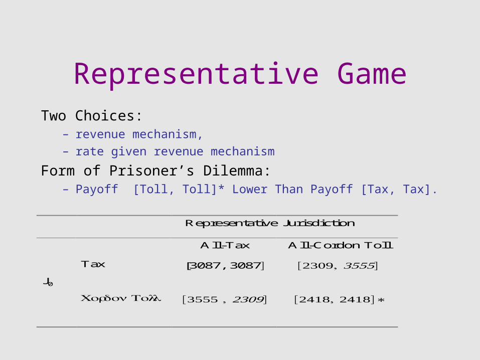
Representative GameTwo Choices:
– revenue mechanism, – rate given revenue mechanism
Form of Prisoner’s Dilemma: – Payoff [Toll, Toll]* Lower Than Payoff [Tax, Tax].
Representative Jurisdiction
All-Tax All-Cordon Toll
J0
Tax [3087, 3087] [2309, 3555]
Cordon Toll [3555 , 2309] [2418, 2418]∗
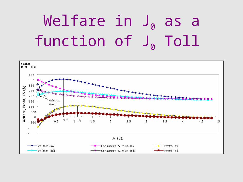
Welfare in J0 as a function of J0 Toll
-1500
-1000
-500
0
500
1000
1500
2000
2500
3000
3500
4000
0 0.5 1 1.5 2 2.5 3 3.5 4 4.5 5
J 0 Toll($/ Crossing)
Welfare-TaxEnvironment
Consumers' Surplus-TaxEnvironment
Profit-TaxEnvironmentWelfare-Toll
EnviornmentConsumers' Surplus-TollEnvironment
Profit-TollEnvironment
W* *
CollectionCosts
Welfare(W, U, Π) ($)

Welfare in J0 at Welfare Maximizing Tolls vs.
Jurisdiction Size in an All-Tax Environment
Welfare (W*, U*, *)($)
-100.00
0.00
100.00
200.00
300.00
400.00
500.00
1 10 100 1000
Size(km)
W-Toll/k m Π/k m U/km W-Tax/ km

Welfare in J0 at Welfare Maximizing Tolls vs.
Jurisdiction Size in an All-Toll Environment
-100.00
0.00
100.00
200.00
300.00
400.00
500.00
1 10 100 1000
Size(km)W-Toll/k m /k m /U k m W-Tax/ km
Welfare(W*, U*, Π*)($)

Tolls by Location of Origin and Destination.
G-+
a bJ0 J+1 J+2
-oo oo
2rτ+2r τ
2rτ+4r τ
2rτ+6r τ
Toll
K -1exit K 0
ent K 0exit K+1
ent K+1exi K+2
ent K+2exi K+3
ent
rτ+r τ
rτ+r τ
0

Policy Choice as a Function of Fixed Collection Costs and
Jurisdiction Size
0
100
200
300
400
500
600
700
800
1 10 100 1000
Size(km)
CCF' - Tax Environment CCF' - Toll Environment CCF - Empirical
Always Tax
Always Toll
Toll if EnvironmentAll-Tax,Tax if EnvironmentAll-Cordon Toll
Fixed CollectionCosts ($)

Policy Choice as a Function of Variable Collection Costs and
Jurisdiction Size
0
0.2
0.4
0.6
0.8
1
1.2
1.4
1 10 100 1000
Size(km)
Theta - Empirical Theta' - Tax Environment Theta' - Toll Environment Toll - Tax Environment Toll - Toll Environment
Always Tax
Always Toll
VariableCollection Cost,Toll ($)

Reaction Curves: Best J0 Toll as Tolls Vary in Toll Environment
0.00
0.20
0.40
0.60
0.80
1.00
1.20
0.00 0.20 0.40 0.60 0.80 1.00 1.20
Toll Environment($)
Toll J0($)
-J urisdiction Size=10km
W-J urisdiction Size=10km-J urisdiction Size=1
kmW-J urisdiction Size=1km

Uniqueness, Non-Cooperative Welfare Maximizing J0 Toll as Initial Toll for
Other Jurisdiction Varies in Toll Environment
-2
0
2
4
6
8
10
12
0 1 2 3 4 5
Iteration#S=-1 S=0 S=1 S=10
Toll ($)
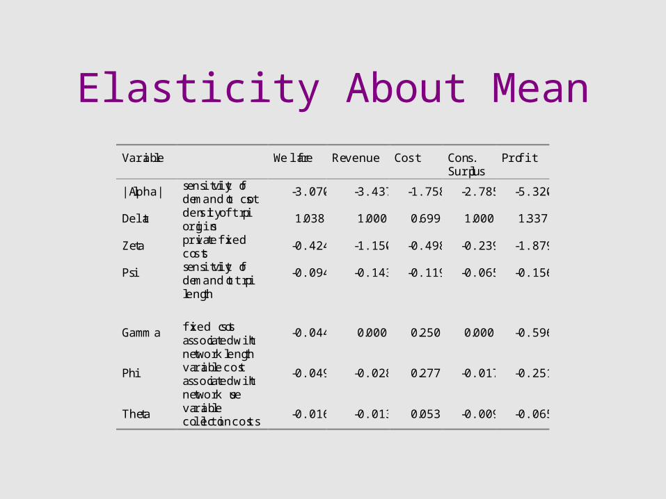
Elasticity About Mean
Variable Welfare Revenue Cost Cons.Surplus
Profit
|Alpha| sensitivity ofdemand to cost
-3.070 -3.437 -1.758 -2.785 -5.320
Delta density of triporigins
1.038 1.000 0.699 1.000 1.337
Zeta private fixedcosts
-0.424 -1.150 -0.498 -0.239 -1.879
Psi sensitivity ofdemand to triplength
-0.094 -0.143 -0.119 -0.065 -0.156
Gamma fixed costsassociated withnetwork length
-0.044 0.000 0.250 0.000 -0.596
Phi variable costassociated withnetwork use
-0.049 -0.028 0.277 -0.017 -0.251
Theta variablecollection costs
-0.016 -0.013 0.053 -0.009 -0.065

Comparison of Tolls and Welfare for Different
Jurisdiction Sizes
Jurisdiction Size (km) Tolls Welfare
10 $0.65 2367
2x10 $1.30 4734
20 $0.68 5451

Rate of Toll Under Various Policies
Environment Policy
tax toll
J0
tax rτχχ = 0 rτ
χχ = 0 rτχτ = 0 rτ
χτ = rτ
∗ττ
Policy toll rττχ = rτ
∗τχ rττχ = 0 rτ
ττ = rτ∗ττ rτ
ττ = rτ∗ττ

General Trip Classification
Section of Destination (y)S- J0 S+
S- G-- G-0 G-+
Section of Origin (x) J0 G0- G00 G0+
S+ G+- G+0 G++

ConclusionsNecessary Conditions For Tolls to Become
Widespread, Need:» Relatively Low
Transaction Costs,» Sufficiently Decentralized
(Local) Decisions About Placement of Tolls.
Actual Conditions Policy Environment
Becoming More Favorable to Road Pricing:» Localized Decisions
(MPO), » Federal encouragement
(ISTEA 2 pilot projects), » Longer trips, » Lower transaction costs
(ETC).


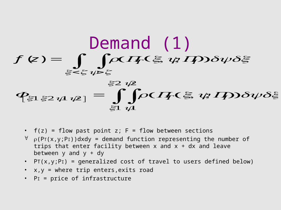
Demand (1)
• f(z) = flow past point z; F = flow between sections (PT(x,y;PI))dxdy = demand function representing the number of trips
that enter facility between x and x + dx and leave between y and y + dy
• PT(x,y;PI) = generalized cost of travel to users defined below)• x,y = where trip enters,exits road• PI = price of infrastructure
f (z) = PT (x,y;PI )( )dydxy>z∫
x<z∫
Fx1x2y1y2[ ] = PT x,y;PI( )( )dydxy1
y2
∫x1
x2
∫

Demand (2)
• PT=total user cost• PI=vector of price of infrastructure α =coefficient (relates price to demand), α < 0 δ = coefficient (trips per km (@ PT =0)), δ > 0 ζ = fixed private vehicle cost = variable private vehicle cost per unit distance• x,y = location trip enters, exits road• VT = value of time• SF = freeflow speed• | | indicates absolute value
PT x, y; PI( )( ) = δeα PT x, y;PI( )
PT x, y; PI( ) =PI + ζ +υ y−x( ) + VTy−xSF
⎛
⎝ ⎜ ⎞
⎠ ⎟

Consumers’ Surplus
U - denotes consumer’s surplusa,b - jurisidction bordersn - counter for tollbooths crossedd - spacing between tollbooths
U0 = PT x, y;p( )( )
PI
∞
∫ dpdydxx
b
∫a
b
∫
+ PT x,y;p( )( )
PI
∞
∫ dpdydxnd
n+1( )d
∫a
b
∫n=1
∞
∑

Model Outcomes
• As the size of jurisdiction J0 increases, that is as |b-a| gets large:
1. F-0 / F-+ increases.
2. F 0+ / F-+ increases.
3. The total number of trips originating in or destined for jurisdiction J0 (F00, F
0+, and F-0) increase.

Transportation RevenuePolicy in J0 Total Revenue
General Tax (χ)
($)
0
Cordon Tolls (τ)
($/Crossing)rτ f ( zk )
k =1
K
∑
Odometer Tax (ω)
($/km)y − x( )rω P T x ,y, P I( )( ) ∂y∂ x
x
∞
∫a
b
∫
Perfect Toll (π)
($/km)y − x( ) rπ P T x ,y , P I( )( )∂ y∂ x
x
b
∫a
b
∫ +
b − x( ) rπ P T x ,y ,P I( )( ) ∂ y∂x
b
∞
∫a
b
∫ +
y − a( )rπ P T x ,y, P I( )( )∂y∂x
a
b
∫−∞
a
∫ +
b − a( )rπ P T x ,y , P I( )( )∂y∂x
b
∞
∫−∞
a
∫

Total Network Cost
where:CT = Total Cost
CCV = Variable Collection Cost
CCF = Fixed Collection Cost
C = Variable Network Cost
CS = Fixed Network Costγ θ κ = model coefficients
CT a,b, Ki( )=CS+C +CCV +CCF
=γ b−a+ f(z)dzz=a
z=b
∫ +θ f(zk)dzk=1
Ki
∑ +κKi

Tolls in All-Cordon Environment
G-+
a bJ0 J+1 J+2
-∞ ∞
2rτ+ 2r τ
2rτ+ 4r τ
2rτ+ 6 r τ
Toll
K -1exit K 0
ent K 0exit K+1
ent K+1exi K+2
ent K+2exi K+3
ent

Price of InfrastructurePolicy User Group Amount paid
to J0
Amount paidoutside J0
General Tax (χ) All 0 0
Cordon Tolls (τ) G00 0 0
G0+, G-0 rτ rτ 2n−1( )
G-+ 2rτ rτ 2n−2m−2( )
Odometer Tax (ω) G00, G0+ rω y−x( ) 0
G-0, G-+ 0 0
Perfect Toll (π) G00 rπ y−x( ) 0
G0+ rπ b−x( ) rπ y−b( )
G-0 rπ y−a( ) rπ a−x( )
G-+ rπ b−a( ) rπ y−b( ) + rπ a−x( )

Rate of Toll Under Various Policies
Enviro nment
tax toll
J0
tax rτχχ = 0
rτχχ = 0
rτχτ = 0
rτχτ
= rτ∗ττ
Policy toll rττχ = rτ∗τχ
rττχ = 0
rτττ = rτ∗ττ
rτττ = rτ∗ττ

Odometer Tax
Rω = rω y−x( )δeα rω y−x( )+ζ +ψ y−x( )( )dydx
x
∞
∫a
x
∫
CT =δφeαζ b−a( )
α rω +ψ( )( )2 +γ b−a( )
Uω =δeαζ b−a( )α 2 rω +ψ( )( )


