CEE 3604: Introduction toTransportation Engineering

Applications of Linear Regression

Drs. H. Baik and A. TraniSpring 2004

CEE 3604 Slide 2

The Basic Question

Suppose we have 10 datapoints, (i.e., n=10)

What is the equation of a line,y = ax + b, that representsthese data points?

Procedure: Find parameters a and b. Estimate the goodness of this fit

>>(R2)

x (=time, min.) y_obs (=temp, K)

0 298

1 299

2 301

3 304

4 306

5 309

6 312

7 316

8 319

9 322

CEE 3604 Slide 3

Find Parameters a and b in y = ax+b.

Minimize Prediction Error (or Sum of the Square ofthe Deviation, SSD)

!

!!

=

==

""=

+=

=

"==

n

1i

2

i

obs

i

ii

pred

i

n

1i

2pred

i

obs

i

n

1i

2

))bax(y SSD i.e.,

b.ax y eq. line thefrom obtained

for x y of valuepredictedy where,

)y(yError)n (PredictioSSD

y = ax + b

yiobs

yipred

(=axi+b)

xi

We like to minimize SSD by selecting appropriatevalues of coefficients a & b.

CEE 3604 Slide 4

Normal Equations to Find a and b

To minimize SSD

! !!

! ! !!

= ==

= = ==

+=="=#

#

+=="=#

#

=#

#=

#

#

n

1i

n

1i

i

obs

i

n

1i

i

obs

i

n

1i

n

1i

n

1i

i

2

i

obs

iii

n

1i

i

obs

i

(2) bn xay 0,1)(b)-ax-(y2b

SSD

(1) xbxa yx 0,)x(b)-ax-(y2a

SSD

0b

SSD

a

SSD

)))bax(y(n

1i

2

i

obs

i!=

""=

! !

! ! !

! !

! ! !

! ! !! !!

= =

= = =

= =

= = =

= = == ==

""#

$%%&

'(

=

""#

$%%&

'(

=

))*

+

,,-

.""#

$%%&

'(=/(/

n

1i

2n

1i

i

2

i

n

1i

n

1i

n

1i

i

obs

i

obs

ii

n

1i

2n

1i

i

2

i

n

1i

n

1i

n

1i

i

obs

i

obs

ii

n

1i

n

1i

2n

1i

i

2

i

n

1i

n

1i

i

obs

i

obs

ii

n

1i

i

xn

1x

xyn

1-yx

xxn

xy-yxn

a so,

xxna xy-yx :x(2)n(1)

n

xay

b :(2) From

n

1i

n

1i

i

obs

i! != =

"

=

CEE 3604 Slide 5

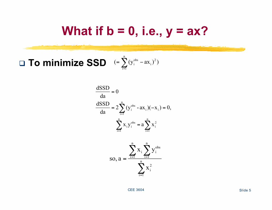
What if b = 0, i.e., y = ax?

To minimize SSD

xa yx

0,)x()ax-(y2da

dSSD

0da

dSSD

n

1i

n

1i

2

i

obs

ii

i

n

1i

i

obs

i

! !

!

= =

=

=

="=

=

))ax(y(n

1i

2

i

obs

i!=

"=

x

yx

a so, n

1i

2

i

n

1i

obs

i

n

1i

i

!

!!

=

===

CEE 3604 Slide 6

An Example for Finding a & b

Many ways to find a & b:Using a spreadsheet like Excel to compute a

and b the long way using equations shownin slide 4 of this handout

Using the ‘Trend Line’ in chart optionUsing tools\data analysis\Regression

Use Matlab curve fit analysis procedure

An example

CEE 3604 Slide 7

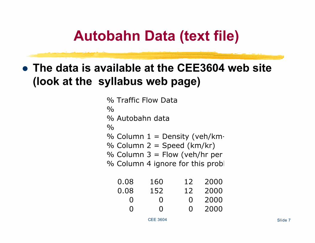
Autobahn Data (text file)

% Traffic Flow Data

%

% Autobahn data

%

% Column 1 = Density (veh/km-lane)

% Column 2 = Speed (km/kr)

% Column 3 = Flow (veh/hr per lane)

% Column 4 ignore for this problem

0.08 160 12 2000

0.08 152 12 2000

0 0 0 2000

0 0 0 2000

The data is available at the CEE3604 web site(look at the syllabus web page)

CEE 3604 Slide 8

Autobahn Data (plot density vs. speed)

Data courtesy of Dr. H. Rakha (Virginia Tech Transportation Institute)

CEE 3604 Slide 9

Linear Regression Model Questions

Can we develop a simple linear regressionmodel to fit 3,000 data points?

How good is the model? Use the model to execute some travel time

calculations

CEE 3604 Slide 10

Procedures

Import the text file in Excel Make a plot Use the trend line procedure Use the regression procedure

CEE 3604 Slide 11

Importing Data Use standard “open” menu in Excel Navigate to the file Follow the import “Wizard”

CEE 3604 Slide 12

Making a Plot

Use the chart “Wizard” to make a plot ofcolumns 1 and 2 of the data file

Always label accordingly Remember units of each axis

CEE 3604 Slide 13

Adding a Trend Line (linear)

CEE 3604 Slide 14

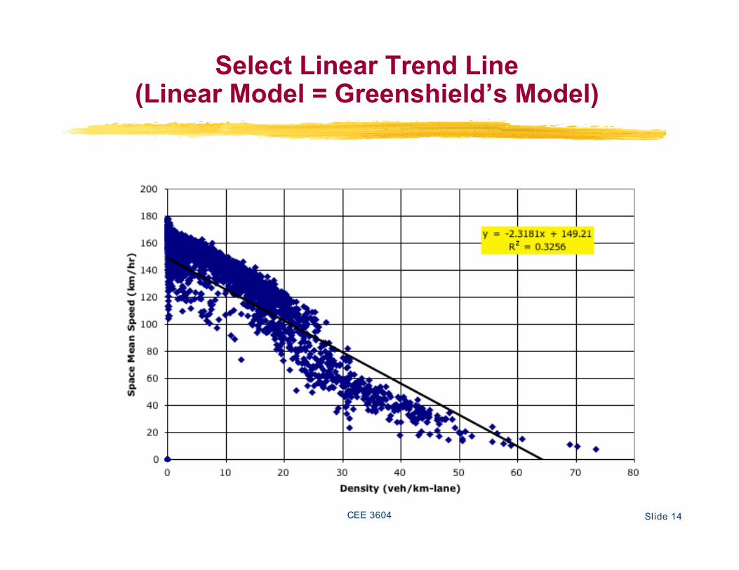
Select Linear Trend Line(Linear Model = Greenshield’s Model)

CEE 3604 Slide 15

Interpretation of Results

The equation of the density vs. speed relationship is:

Y-intercept is free flow speed (Uf) X-intercept (or the zero of the line) is the jam density (kj) Uf = 149.21 km/hr and kj = 149.21/2.32 = 64.3 veh/km per

lane

CEE 3604 Slide 16

Traffic Flow Equations

and Flow is,

also,

CEE 3604 Slide 17

Plot and Compare with Data

CEE 3604 Slide 18

Plot and Compare Data with Curve Fit

CEE 3604 Slide 19

Interpreting the Data

The Greenshield’s model is a modest approximation ofthe data

The parabola of speed and flow in the Greenshield’smodel seems to “lag” behind many of the data pointsfrom the field

However, note that peak flow (qmax) seems to be areasonable value at 2,300 veh/hr considering the highspeeds of the road

The parabola relating density and flow is very good forlow values of density (no congestion)

CEE 3604 Slide 20

Using the Regression Procedure

Here we use Excel Data Analysis module toanalyze the data

The Data Analysis is found under menu “Tools”and “Data Analysis”

Linear regression

CEE 3604 Slide 21

Executing the Regression

Regression Coefficients

CEE 3604 Slide 22

Quick Regression in Matlab

Matlab has basic curve fitting capabilities justlike Excel trend line analysis

Make a plot and the “Curve Fitting” command islocated in the “Tools” pull-down menu

Another more advanced method to performleast squares is to use the “polyfit” commandto fit a polynomial to a data

See some examples in the pages that follow

CEE 3604 Slide 23

Matlab Curve Fitting Setup

Curve Fitting Selection

CEE 3604 Slide 24

Matlab Curve FittingCurve Fitting Selection

Window

CEE 3604 Slide 25

R2

R2 (Coefficient of determination)

!

!

=

=

"

"

"=

=

=

=

n

1i

2obs

i

n

1i

2pred

i

obs

i

2

)y(y

)y(y

1

variationTotal

. variationdUnexplaine-1

variationTotal

variationed Unexplain- variationTotal

average) the(from variationTotal

eq.)(by variationExplainedR

yy

y

x

Total

Variance

(from the

average)

yiobs

yipred

y = ax + b

Explained

Variance

(by the Eq.)

Unexplained

Variance

An Example

CEE 3604 Slide 26

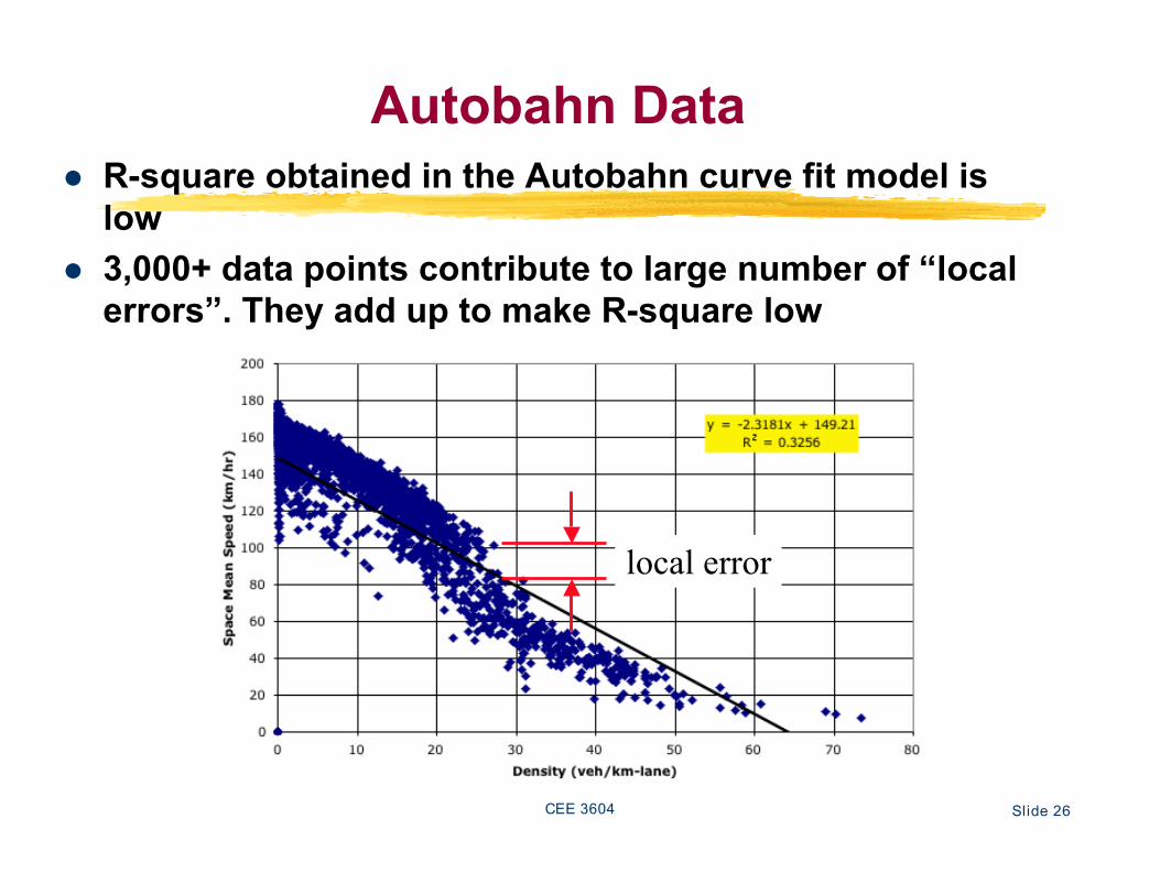
Autobahn Data R-square obtained in the Autobahn curve fit model is

low 3,000+ data points contribute to large number of “local

errors”. They add up to make R-square low

local error

CEE 3604 Slide 27

Traffic Data Analysis

One morning the video cameras of the Autobahn recordan average of 25 vehicles per km per lane. What is thetravel time between two 3 km. exit ramps?

Solution: At k = 25 veh/km-lane we have,

The travel time is then 1.98 minutes Travel time estimations can be easily done using any

one of the traffic flow models discussed in class

CEE 3604 Slide 28

Graphical Solution

CEE 3604 Slide 29

Sy⋅x

Sy⋅x (Standard error ofestimation of y on x) A measure of the

scatter of the datapoints about theregression curve.

!!"

#$$%

&''=

''=

'==

( ( (

(

(

= = =

=

=

)

n

1i

n

1i

n

1i

obs

ii

obs

i

2obs

i

n

1i

2

i

obs

i

n

1i

2pred

i

obs

ixy

yxbya)(yn

1

b)ax(yn

1

)y(yn

1SSD

n

1S

CEE 3604 Slide 30

Sy⋅x (Standard error of estimation of y on x)

If we construct linesparallel to the regressionlines at respective verticaldistances of Sy⋅x, 2Sy⋅x and3Sy⋅x from it, we shouldfind 68%, 95% and 99.7%of the observed (sample)data points assuming wehave a large enough datapoints.

y y = ax + b

Sy.x

3Sy.x

2Sy.x

x

CEE 3604 Slide 31

rxy

rxy (Coefficient ofcorrelation) A measure of the

linearity of the data Same as the square root

of R2

)y(y)x(xn

1S

)y(yn

1S

xofdeviation standard ,)x(xn

1S where,

,SS

S

y) of x)(sdof (sd

y &between x covariancer

obs

i

n

1i

ixy

n

1i

2obs

iy

n

1i

2

ix

yx

xy

xy

!!=

!=

!=

==

"

"

"

=

=

=

In statistics, variance = mean of variation covariance = mean of covariation

CEE 3604 Slide 32

rxy (Coefficient of correlation)

y

x

y

x

rxy

> 0

y

y

x

rxy

< 0

y

y

x

rxy

~0

xx

y

rxy

=1

(perfect positive relation)

x

y

rxy

=-1

(perfect negative relation)

y

rxy

= 0

(nonlinear relation)

)y(y)x(xn

1S obs

i

n

1i

ixy!!= "

=

CEE 3604 Slide 33

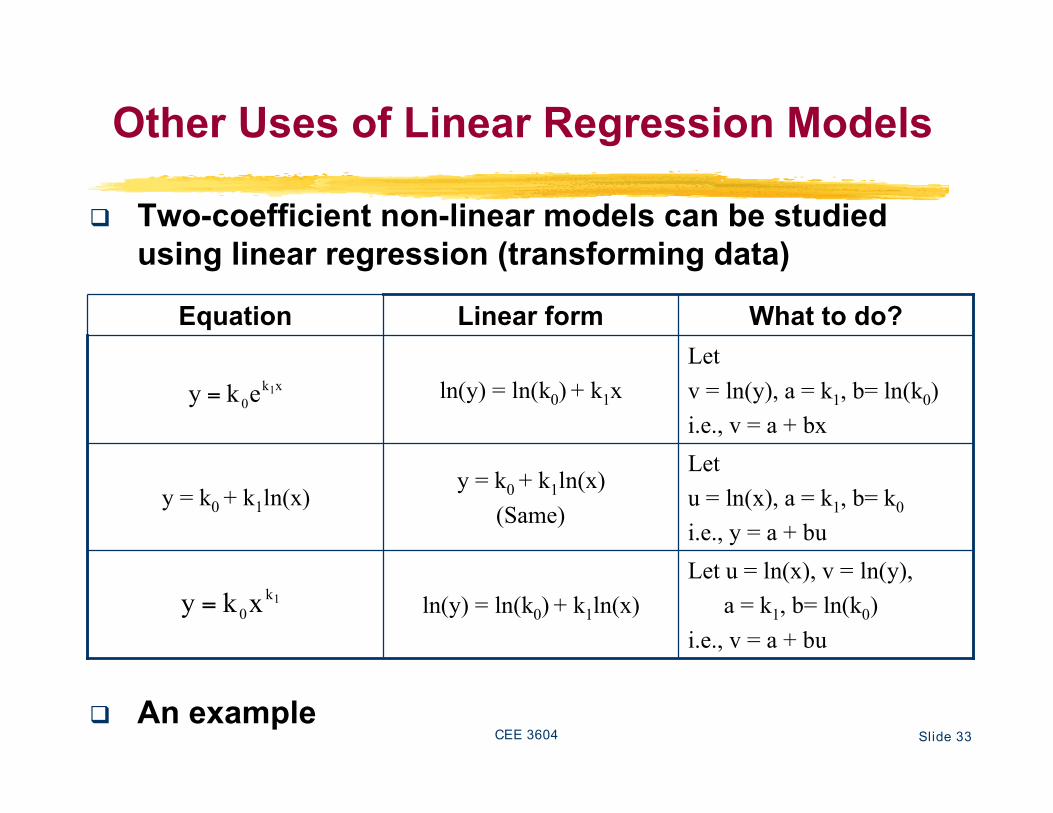
Other Uses of Linear Regression Models

Two-coefficient non-linear models can be studiedusing linear regression (transforming data)

An example

Let u = ln(x), v = ln(y), a = k1, b= ln(k0)i.e., v = a + bu

ln(y) = ln(k0) + k1ln(x)

Letu = ln(x), a = k1, b= k0

i.e., y = a + bu

y = k0 + k1ln(x)(Same)

y = k0 + k1ln(x)

Letv = ln(y), a = k1, b= ln(k0)i.e., v = a + bx

ln(y) = ln(k0) + k1x

What to do?Linear formEquation

xk

01eky =

1k

0xky =

CEE 3604 Slide 34

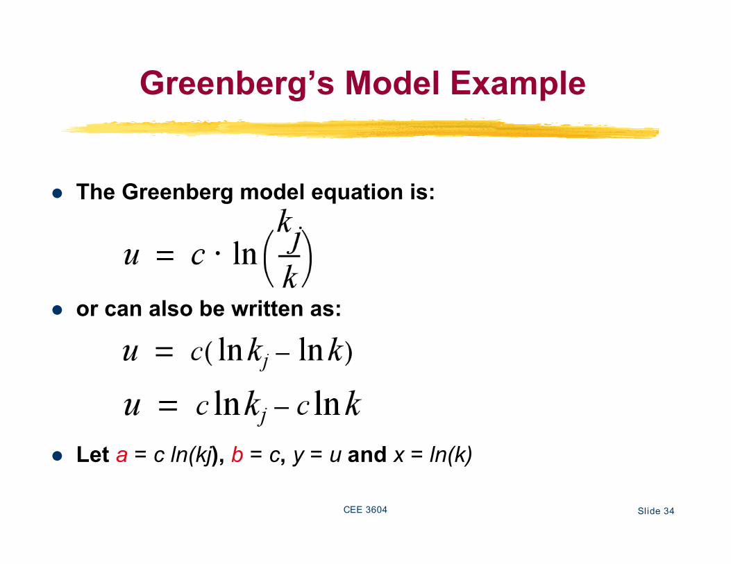
Greenberg’s Model Example

The Greenberg model equation is:

or can also be written as:

Let a = c ln(kj), b = c, y = u and x = ln(k)

CEE 3604 Slide 35

Greenberg’s Model Example

Then the original non-linear equation has been“linearized”

The important issue is that to do a linear regression ofthe data according to Greenberg’s model we need totake the natural logarithm of the data (x = ln(density))

We regress u against ln(k) and obtain a linearrelationship

!

y = a " bx

CEE 3604 Slide 36

Field Data for Greenberg’s Model

Greenberg Model

Vs (km/hr) k (veh/km-la) ln(k)

161.7 9.5 2.25

153.02 11.4 2.43

153.75 11.5 2.44

81.33 18.74 2.93

138.84 12.71 2.54

122.5 15.58 2.75

115.35 20.39 3.02

95.22 25.83 3.25

67.68 30.67 3.42

20.67 43.54 3.77

54.4 25.15 3.22

10.18 58.94 4.08

35.63 35.03 3.56

18.15 42.98 3.76

20.2 49.9 3.91

15.19 50.56 3.92

CEE 3604 Slide 37

Plot of k versus Vs Observe the relationship as non-linear An exponential trend line has been added to

make the point

CEE 3604 Slide 38

Plot of ln(k) versus Speed (Vs)

CEE 3604 Slide 39

Things to Observe

The regression model works quite well for a small dataset that is not linear

We have transformed the variable density (k) and usedln(k) instead

The new model is:

The model is of the form:

The value of kj can be obtained using the first term andequating it to 369.42