Abstract—Evaluation the coverage area in a wireless

network is very important for cellular system designers in order to provide good service to users. It is hard to collect the Receive Signal Level (RSL) for an entire coverage area because of many obstacles, such as buildings, lakes, and vegetation, so that the estimation of the coverage area is essential for locations for which it is difficult to measure the RSL. Also, estimating the coverage area can help to reduce the consumption of time and money. Kriging is a well-known method of estimating unknown values at specific locations, and it has shown accurate results. This paper discusses the estimation of a coverage area in Melbourne, FL by using Kriging. The distance factor in Kriging has never been studied before. A drive test is used to collect RSL measurements, and they are gathered in different distance sizes, a procedure known as binning, to shape the coverage area. In this case, Kriging is used to estimate the coverage area in bin sizes that are 200x200, 100x100, 50x50, and 25x25 meters of resolution.

Index Terms— kriging; coverage estimation; coverage map; binning; spatial statistics

I. INTRODUCTION HE cell coverage area is one of the most important factors in cellular communication system designs. It may

be defined as the largest distance that a cell phone can be away from the base station while still maintaining an acceptable service [1]. The base station is usually located near the center of the required served area [2].

A. Cell Coverage Area Any cellular system network is comprised of several cells.

They are connected together to provide radio coverage over a larger geographical area. The cell coverage area allows a large number of users to communicate with each other and with fixed base stations in the cellular network. These base stations provide connections to transceivers regardless of their mobility, whether they are moving across cells or are stationary. The extent of cell and network coverage depends mainly on natural factors, such as propagation conditions, and human factors, such as the landscape (urban, suburban, rural), subscriber behavior, etc. [3].

Abdlmagid Basere is a Ph.D Candidate in the Electrical and Computer

Engineering Department, Florida Institute of Technology, Melbourne FL 32901 USA (Phone: 321-525-9206, email:abasere2011@my.fit.edu).

I. Kostanic is with the Electrical and Computer Engineering Department, Florida Institute of Technology, Melbourne FL 32901 USA (Phone: 321-674-7189, email:kostanic@fit.edu).

B. Importance of Understanding Cell Coverage Area 1) Coverage Planning: Coverage planning procedure

may be divided into three phases. The first phase is called the preplanning phase. In this phase, the general properties of the future network are investigated. In the second phase, the site survey for the targeted coverage area and an investigation of possible base stations’ locations are performed. Then, constant modification is made to move the network planning forward. In the final phase, driving test data collection is done repeatedly in order to examine the coverage area until good coverage is guaranteed. After that, the system is ready to be deployed in the target area to provide service [4].

2) Concept of Handoff: Handoff is an operation that allows a mobile user to move from one cell to another without interruption of service. The handoff procedure can be implemented based on many conditions such as interference levels and signal strength [5].

3) Interference: Interference occurs when neighboring cells operate on the same frequency at the same time. One of the main impairments that can limit performance of a cellular system in the multi-cell network is the inter-cell interference. Interference causes background noise and bad voice quality when a call is in progress. In this case, the coverage area determination is helpful to eliminate interference, leading to higher quality of service [6].

4) User Location: The mobile telecommunication network contains many base stations (BSs) which offer mobile telecommunication service to mobile users. Each BS represents a cell that is providing coverage to a particular area, and each cell is divided into sectors. Understanding the coverage of the sectors helps locate the users that are within systems service area [7].

C. Methods for Estimating Cell Coverage A There are many methods of performing the estimation

of coverage areas, and each of them has their own benefits and drawbacks, but none of them is 100% accurate [8]. Three performance estimation methods are described as follows.

1) Geometry: There are many methods of computational geometry. The Voronoi diagram is one of the most important data structures in computational geometry, and there are three reasons for its usefulness. First, Voronoi diagrams are seen in nature in many cases. Certainly, some natural processes may be used to describe specific classes of Voronoi diagrams. Human understanding is facilitated by visual perception. For example, if one grasps the underlying structure of anything, its complete status might be understood at an advanced level. Second, Voronoi diagrams

Cell Coverage Area Estimation From Receive Signal Level (RSL) Measurements

Abdlmagid Basere, Ivica Kostanic

T

Proceedings of the World Congress on Engineering and Computer Science 2016 Vol I WCECS 2016, October 19-21, 2016, San Francisco, USA

ISBN: 978-988-14047-1-8 ISSN: 2078-0958 (Print); ISSN: 2078-0966 (Online)

WCECS 2016

have amazing and exciting mathematical properties; for example, they are linked to many famous geometrical structures. As a result, some authors consider that “the Voronoi diagram is one of the most fundamental constructs defined by a discrete set of points” [9]. Lastly, Voronoi diagrams have been shown to be a strong tool in solving unconnected computational problems. In the last few years, Voronoi diagrams have caught the interest of computer scientists [9].

However, algorithms that use Voronoi diagrams to estimate coverage areas do not take into consideration the features of the propagation environment, and they oversimplify the coverage problem [10]. For this reason, among others, the use of Voronoi diagrams is not being followed in this work.

2) Prediction: One of the most elementary tasks in the cellular system design is propagation modeling and coverage prediction. Over many years a variety of approaches have been used to predict coverage areas using propagation models. These models are helpful in predicting path loss or signal attenuation, thus enabling acceptable reception [11]. Cellular designers usually use advanced planning tools for network coverage estimation. The coverage estimation is based on terrain data combined with a propagation model [12].

3) Measurements: Drive tests are normally used for collecting the Receive Signal Level (RSL). Because carrying out driving tests is time consuming and expensive, there is significant interest in improving the quality of coverage estimation that is obtained from a limited number of driving test measurements. The problem with drive test measurements is that data cannot be conducted in the whole region of the network because of many obstacles [12] such as buildings, lakes, and vegetation. In this case, the estimation of the coverage area is important and can rely on spatial prediction techniques such as Inverse Distance Weighting, Kriging, and Artificial Neural Networks.

II. LITERATURE REVIEW

A. Data Collection Verification of cellular system coverage requires the RSL

measurements that can be collected by spatial averaging of immediate signal power readings. The measurements are typically gathered in conformity with the well-known Lee sampling criteria [13]. Equation 1 describes the amplitude of the received signal envelope in the mobile propagation environment [13].

)x(r)x(m)x(r 0= (1)

It is reasonable to denote the received signal by a

stationary stochastic process, where )x(r0 represents the fast fading variation of a mean signal strength value equal to 1. The mean value of the signal envelope is )x(m , and x is the location of the local mean [14].

There are two questions that need to be answered in order to get an estimate that is statistically valid for the local mean. First, how many ‘snapshots’ of the received signal level are required to be collected over a suitable distance, in order to

assure the statistical validity of the approximation, and second, what would be an appropriate spatial distance to average over. The space averaging over a distance should be performed in order to guarantee averaging Rayleigh fading effects. Estimation of the local mean can be characterized as an average of the power of the signal over a appropriate distance ( 2L ) as shown in equation 2 [15]:

∫∫+

−

+

−

==Lx

Lx

Lx

Lx

dy)y(r)y(mdy)y(rL

)x(p 20

22

21 (2)

keeping L2 small enough so that xm)y(m ≈ over [ ]Lx,Lx +− The variance of the power estimate is given as [14].

avx

x

Lx

Lx

x pm

)x(rmdy)y(rL

m)x(p ==×≈= ∫

+

−π

22

022

0

2 42

(3)

dxm)x(RmLx

L rx

L

p

−

−= ∫ 4

44

2

0

2 162

121

20 π

σ (4)

where )x(R 2

0r is the autocorrelation function of 2

0r given by

+=

λπ

πxJ)x(Rr

2116 2022

0

(5)

Equation (4) has been statistically evaluated [2] for

different values of L , and the results for σ1 and σ2 spreads are shown in Table I [15].

For most practical situations, terrain variations (shadowing) over a λ40 distance can be assumed to be negligible, and, therefore, the assumption that the mean value of the signal is not changeable during the integration in equation (3) is valid [15].

“Macroscopic propagation models predict the mean received signal level over a small geographical area called a bin” [15]. The bin’s size is calculated as a function of accuracy and the database terrain resolution, computation time, roughness of the terrain, etc. and usually ranges from 50m to 500m. The local area mean (LAM) is the mean received signal of a bin. Performing averaging of several

TABLE I SPREAD OF THE LOCAL MEAN ESTIMATE AS A FUNCTION OF THE

AVERAGING DISTANCE L2 pσ σ1 Spread

σ−

σ+

pav

pavpp

log

σ2 Spread

σ−

σ+

pav

pav2p2p

log

λ5 avp33.0 dB98.2 dB5.6

λ10 avp24.0 dB14.2 dB5.4

λ20 avp18.0 dB55.1 dB24.3

λ40 avp12.0 dB1 dB1.2

Proceedings of the World Congress on Engineering and Computer Science 2016 Vol I WCECS 2016, October 19-21, 2016, San Francisco, USA

ISBN: 978-988-14047-1-8 ISSN: 2078-0958 (Print); ISSN: 2078-0966 (Online)

WCECS 2016

local means can allow comparing measurement data with the predictions of the propagation model [15].

During driving through a particular bin, the measurement equipment implements the collection of the local means within the bin. The local means tend to comply with a normal distribution in the logarithmic domain with a standard deviation σ and mean value m . The local area mean for the specific bin is calculated as an average value of the local means collected in that specific bin.

N

LL

N

kMk

AM

∑== 1 (6)

where AML is the local area mean, MkL represents the thk local mean and N is the total number of local means collected in the bin [15].

B. Spatial Binning In order to enable users to understand how the data are

changing between the temporal bins, spatial binning is essential. Spatial binning gathers data points that are near one another to prevent the situation in which data points share the same location in space. Both Longitude and Latitude contain numeric information. A simple grid is used in the binning procedure; the resolution is controllable by the users [16].

Insufficient drive test data can cause inaccurate estimation of coverage area. However, collection of too much data is costly and time consuming. Combining data by averaging can help with reducing the processing load and quantifying data to the resolution of a specific terrain, which is referred to as the bin of the area [15].

C. Interpolation Methods Through interpolation, one-use measurement data samples

can be collected and used to estimate measurement data at other points where measurement data are not available. The most popular spatial interpolation methods are Kriging, spline interpolation, interpolating polynomials, and Inverse Distance Weighting (IDW) [17]. Among the above methods, IDW and Ordinary Kriging (OK) are the most commonly used, and are typically the most frequently suggested interpolation techniques [18].

“Kriging is an interpolation technique based on the methods of geostatistics” [19]. Krige (1951) collected samples over mining fields and used them to develop optimal interpolation methods for use in the mining industry. Nowadays, the Kriging method is being used in soil mapping, groundwater modeling [20], [21], and in many other spatial problems [20].

III. PROPOSED APPLICATION

A. Kriging Method The principle interpolation equation in the Kriging model

is given by [19].

∑=

=n

iii )x(z.)x(z

10 λ (7)

where )x(z i is the measured value at the thi location, iλ is an unknown weight for the measured value at the

thi location, and )x(z 0 is the prediction location. As seen, at the point where the algorithm performs the

interpolation the value is obtained as a weighted average from the points in the immediate neighborhood. The most significant task associated with the implementation of (7) is the determination of the appropriate weights. The fitted variogram is used to determine the weights iλ that are required for local interpolation. The estimation )x(z 0 may be unbiased by choosing the weights iλ . Predicting numerous locations may give some values which could be below the real values and some above, so the sum of weights

iλ must be equal to 1 in order to guarantee that the prediction of the unknown measurement is unbiased [20].

∑=

=n

ii

1

1λ (8)

1) Semivariogram: “The variogram characterizes the

spatial continuity or roughness of a data set. Usually, one dimensional statistics for two data sets might be equal” [19]. However, the spatial continuity could be dissimilar. The difference between the semivariogram and the variogram is just a factor of 2. The variogram is described as [20].

[ ]22 )(Z)(ZE)( hxxh +−=γ (9)

shows the variogram )( hγ2 of differences between sites which are functions of the distance h between them, where

)(Z x and )(Z hx + are the values of the random variable Z of interest at locations )( x and )( hx + . The function of interest in practice is )( hγ , which is called a semi-variogram and is used in Kriging. The statistical expectation operator is [ ]E . Kriging uses the empirical variogram )( hγ as a theoretical variogram to get the first approximation of the variogram for spatial prediction [20], [22].

{ }2

121 ∑

=

+−=n

iii )hx(z)x(z

n)h(γ (10)

where )x(Z is the value at location ix , )hx(Z i + is the value at location hxi + , and n is the number of pairs of points of observations of the values of attribute separated by distance h ; the plot of )h(γ against h is known as the experimental variogram. The experimental variogram provides useful information for interpolation, optimizing sampling, and determining spatial patterns. It is clear that the number of semi-variogram samples is proportional to the available pairs of locations. When datasets are large, the number of pairs of locations will grow quickly. Therefore,

Proceedings of the World Congress on Engineering and Computer Science 2016 Vol I WCECS 2016, October 19-21, 2016, San Francisco, USA

ISBN: 978-988-14047-1-8 ISSN: 2078-0958 (Print); ISSN: 2078-0966 (Online)

WCECS 2016

the binning of the distance is required in order to get the variogram parameters, which are the sill, the nugget, and the range [20]. Also, the case of the RSL interpolation, the binning of the data is necessary so that the effects of fast fading are reduced.

2) Fitting Variogram Models: The fitting model is obtained by plotting the empirical semivariance )h(γ versus the lag distance (separation distance of the pairs) [23], and it provides specific parameters, namely the sill, the nugget, and the range as shown in Fig. 1.

A variogram model is a parametric curve fitted to a variogram estimator. There are four variogram fitting models that are used in the Kriging method to help interpolate data accurately, and the most commonly used variogram models are summarized as follows [20]:

The remainder of this paper is organized as follows: Section IV gives an overview of experimental verification, which is divided into measurement setup, data collection, and results of interpolation; in Section V, a brief summary and conclusions are provided.

IV. EXPERIMENTAL VERIFICATION The measurements are performed in a study area that is

located in Melbourne, FL. The map of the area is presented in Fig. 3. Although, the study is performed at a specific

frequency; the methodology should be widely applicable across all UHF/VHF frequencies used for personal communication systems. The Melbourne area is a suburban area. For the study, the transmitter is located on the rooftop of a multi-story building, making for good wide area coverage. The majority of houses in the selected area are one to two floors, and their heights range from 4 to 9 meters. Also, there are open areas such as small artificial lakes, parks, and vegetation. The satellite view of the study area is shown in Fig. 3.

A. Data Collection An illustration of the data collection system is presented

in Fig.4. The system consists of the following parts:

1) Transmitter: The transmitter is used to evaluate PCS band signal propagation, and the frequency range is 1.85 to 2.1 GHz, where the power is up to 43 dBm. This transmitter allows the transmission of the signal at the radio frequency of 1925MHz.

2) Transmit Antenna: The transmitter antenna is used in the transmission of signals to be measured. It is an omnidirectional antenna, and its frequency ranges between 1850 MHz and 1990 MHz. It also radiates in a horizontal plane with 6 dBi gain.

3) Receiver: An Agilent Technologies E6474A receiver is used to collect RSL measurements at different spatial points.

γ (h)

Lag (h)

γ (h) vs Lag (h)

Sill

Partial Sill

NuggetEffect

Fig. 1. Simple transitional variogram with range, nugget, and sill

Fig. 3. Satellite view of the studied environment

Transmit antenna

TransmitterGPS

Receiver antenna

ReceiverPC

Fig. 4. Illustration of the measurement system

γ (h

)

Lag (h)

Lag (h) Vs γ (h)

Nugget

Sill

Range

Spherical variogram model

γ (h

)

Lag (h)

Lag (h) Vs γ (h)

Nugget

Sill

Range

Gaussian variogram model

γ (h

)

Lag (h)

Lag (h) Vs γ (h)

Sill

Nugget

Linear variogram model

γ (h

)

Lag (h)

Lag (h) Vs γ (h)

Nugget

Sill

Range

Exponential variogram model

Fig. 2. Examples of most commonly used variogram models

Proceedings of the World Congress on Engineering and Computer Science 2016 Vol I WCECS 2016, October 19-21, 2016, San Francisco, USA

ISBN: 978-988-14047-1-8 ISSN: 2078-0958 (Print); ISSN: 2078-0966 (Online)

WCECS 2016

4) Receiver Antenna: The receiver antenna is used to collect RSL measurements. It is an omnidirectional antenna with a frequency range between 1850 and 1990 MHz.verage Planning: Coverage planning.

5) GPS Antenna: The GlobalSat BU-353-S4 is a USB magnet mount GPS receiver whose characteristics are extreme sensitivity, low power consumption, and an ultra-compact chipset. The BU-353-S4 GPS is appropriate for automotive navigation, marine navigation, mobile phone navigation, personal positioning, and fleet management. It is compatible with Microsoft Windows. A SiRF Star IV GPS chipset is used in this GPS, which delivers high performance in urban canyons as well as in dense foliage. It uses a 48-channel antenna, which allows the receiver to give the highest degree of accuracy. It is connected with the PC to allow JDSU Wireless Solutions software to identify and store the position of measured data in terms of latitude, longitude, and altitude. The stored position helps the user to get the best interpolation of the coverage area.

B. Data Collection and Binning A drive test was performed in the targeted geographic

area, where RF measurements were detected and stored. The measurements that were collected to provide interpolation for gaps are shown in Fig. 5.

The measured data are used to generate a coverage area map for the area. Every spatial point can be described as a point of intersection of both the x-axis and the y-axis, where longitude is the x-axis and latitude is the y-axis. A Matlab code was used to do binning. Since the data set is large, the binning was done for the coverage area as shown in Fig. 6-9 with a different resolution. In this research, the binning is based on the distances, such as 200x200, 100x100, 50x50 and 25x25 meters binning.

Fig. 5. Measured Data of the Study Area.

-80.67 -80.665 -80.66 -80.655 -80.65 -80.645 -80.64 -80.635

28.045

28.05

28.055

28.06

28.065

28.07

28.075

Longitude

Latit

ude

Original Coverage Map (50X50 meters)

-120

-110

-100

-90

-80

-70

-60

Fig. 7. Original coverage area of 50x50 meters resolution

-80.67 -80.665 -80.66 -80.655 -80.65 -80.645 -80.64 -80.635

28.045

28.05

28.055

28.06

28.065

28.07

28.075

Longitude

Latit

ude

Original Coverage Map (100X100 meters)

-105

-100

-95

-90

-85

-80

-75

-70

-65

-60

Fig. 8. Original coverage area of 100x100 meters resolution

-80.67 -80.665 -80.66 -80.655 -80.65 -80.645 -80.64 -80.635

28.045

28.05

28.055

28.06

28.065

28.07

28.075

Longitude

Latit

ude

Original Coverage Map (25X25 meters)

-120

-110

-100

-90

-80

-70

-60

Fig. 6. Original coverage area of 25x25 meters resolution

Proceedings of the World Congress on Engineering and Computer Science 2016 Vol I WCECS 2016, October 19-21, 2016, San Francisco, USA

ISBN: 978-988-14047-1-8 ISSN: 2078-0958 (Print); ISSN: 2078-0966 (Online)

WCECS 2016

Calculating the semivariogram fitting model is done by plotting the empirical semivariogram versus the distance as shown in Fig. 10. The empirical semivariogram cloud shows that the number of pairs of locations will rise quickly when the dataset becomes large.

When the dataset is large, the calculation of the semivariogram fitting model becomes difficult. As a result, the points of the variogram cloud may be gathered into classes of distances ("bins") in order to find the variogram fitting model for the targeted area. The linear fitting variogram model is being the result of the measurements obtained from the collected data as shown in Fig.11.

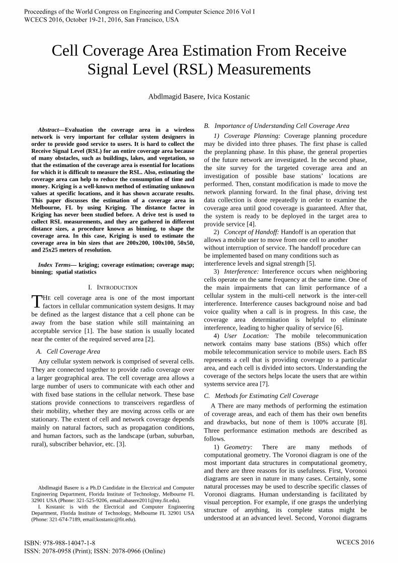
C. Results of Interpolation The interpolation view of the coverage area for 200x200,

100x100, 50x50, and 25x25 meters resolution are shown in Fig. 12-15. The interpolation of the coverage area of 25x25 meters resolution gave more details about RSL, and it is smooth as shown in Fig. 12.

Fig. 10. Empirical semivariogram cloud

-80.67 -80.665 -80.66 -80.655 -80.65 -80.645 -80.64 -80.635

28.045

28.05

28.055

28.06

28.065

28.07

28.075

LongitudeLa

titud

e

Interpolated Coverage Map (25X25 meters)

-120

-110

-100

-90

-80

-70

-60

Fig. 12. Interpolated coverage area of 25x25 meters resolution

-80.67 -80.665 -80.66 -80.655 -80.65 -80.645 -80.64 -80.635

28.045

28.05

28.055

28.06

28.065

28.07

28.075

Longitude

Latit

ude

Interpolated Coverage Map (50X50 meters)

-120

-110

-100

-90

-80

-70

-60

Fig. 13. Interpolated coverage area of 50x50 meters resolution

-80.67 -80.665 -80.66 -80.655 -80.65 -80.645 -80.64 -80.635

28.045

28.05

28.055

28.06

28.065

28.07

28.075

Longitude

Latit

ude

Interpolated Coverage Map (100X100 meters)

-105

-100

-95

-90

-85

-80

-75

-70

-65

-60

Fig. 14. Interpolated coverage area of 100x100 meters resolution

-80.67 -80.665 -80.66 -80.655 -80.65 -80.645 -80.64 -80.635

28.045

28.05

28.055

28.06

28.065

28.07

28.075

Longitude

Latit

ude

Interpolated Coverage Map (200X200 meters)

-100

-95

-90

-85

-80

-75

-70

-65

Fig. 9. Interpolated coverage area of 200x200 meters resolution

Fig. 11. Linear variogram model of study area

Proceedings of the World Congress on Engineering and Computer Science 2016 Vol I WCECS 2016, October 19-21, 2016, San Francisco, USA

ISBN: 978-988-14047-1-8 ISSN: 2078-0958 (Print); ISSN: 2078-0966 (Online)

WCECS 2016

V. SUMMARY AND CONCLUSIONS Measurements of the RSL in the 1925MHz band in a

suburban area were collected. The interpolation of a specific coverage area was done successfully. Measurements show that the semivariogram model is linear. The use of Kriging proves to be very effective. It shows a good result when the coverage area was divided into different bin sizes that are 200x200, 100x100, 50x50, and 25x25 meters of resolution. Likewise, the importance of the exact measurements of the RSL for the binning procedure is shown. The approach looks very promising and it is believed to be worth pursuing at a larger scale.

REFERENCES [1] H. Jiang and C. H. Davis, "Cell-coverage estimation

based on duration outage criterion for CDMA cellular systems," IEEE transactions on vehicular technology, vol. 52, pp. 814-822, 2003.

[2] J. D. Parsons and P. J. D. Parsons, "The mobile radio propagation channel," 2000.

[3] P. K. Sharma and R. Singh, "Cell coverage area and link budget calculations in GSM system," International Journal of Modern Engineering Research (IJMER) vol, vol. 2, pp. 170-176, 2012.

[4] Y. Sun, "Radio Network Planning for 2G and 3G," Master of Science in Communications Engineering, Munich University of Technology, 2004.

[5] K. R. Manoj, "Coverage estimation for mobile cellular networks from signal strength measurements," Citeseer, 1999.

[6] J.-S. Sheu and W.-H. Sheen, "Characteristics and modelling of inter-cell interference for orthogonal frequency-division multiple access systems in multipath Rayleigh fading channels," IET Communications, vol. 6, pp. 3015-3025, 2012.

[7] L. Arigela, P. Veerendra, S. Anvesh, and K. Satya, "Mobile Phone Tracking & Positioning Techniques," International Journal of Innovative Research in Science, Engineering and Technology, vol. 2, 2013.

[8] I. Akbari, O. Onireti, M. A. Imran, A. Imran, and R. Tafazolli, "Effect of inaccurate position estimation on self-organising coverage estimation in cellular

networks," in European Wireless 2014; 20th European Wireless Conference; Proceedings of, 2014, pp. 1-5.

[9] F. Aurenhammer, "Voronoi diagrams—a survey of a fundamental geometric data structure," ACM Computing Surveys (CSUR), vol. 23, pp. 345-405, 1991.

[10] M. Argany, M. A. Mostafavi, F. Karimipour, and C. Gagné, "A GIS based wireless sensor network coverage estimation and optimization: A Voronoi approach," in Transactions on Computational Science XIV, ed: Springer, 2011, pp. 151-172.

[11] S. Sharma and R. Uppal, "RF Coverage Estimation of Cellular Mobile System," Intrnational journal of Engineering and Technology, vol. 3, p. 60, 2011.

[12] B. Sayrac, J. Riihijärvi, P. Mähönen, S. Ben Jemaa, E. Moulines, and S. Grimoud, "Improving coverage estimation for cellular networks with spatial bayesian prediction based on measurements," in Proceedings of the 2012 ACM SIGCOMM workshop on Cellular networks: operations, challenges, and future design, 2012, pp. 43-48.

[13] I. Kostanic, J. Zec, and N. Faour, "Sampling Criteria for Wideband Received Signal Measurements," in International Conference on Wireless Networks, 2003, pp. 24-29.

[14] W. Lee and Y. Yeh, "On the estimation of the second-order statistics of log normal fading in mobile radio environment," IEEE Transactions on Communications, vol. 22, pp. 869-873, 1974.

[15] I. Kostanic, N. Rudic, and M. Austin, "Measurement sampling criteria for optimization of the Lee's macroscopic propagation model," in Vehicular Technology Conference, 1998. VTC 98. 48th IEEE, 1998, pp. 620-624.

[16] O. Hoeber, G. Wilson, S. Harding, R. Enguehard, and R. Devillers, "Visually representing geo-temporal differences," in Visual Analytics Science and Technology (VAST), 2010 IEEE Symposium on, 2010, pp. 229-230.

[17] D. Zimmerman, C. Pavlik, A. Ruggles, and M. P. Armstrong, "An experimental comparison of ordinary and universal kriging and inverse distance weighting," Mathematical Geology, vol. 31, pp. 375-390, 1999.

[18] J. Li and A. D. Heap, "A review of comparative studies of spatial interpolation methods in environmental sciences: Performance and impact factors," Ecological Informatics, vol. 6, pp. 228-241, 2011.

[19] A. Konak, "Estimating path loss in wireless local area networks using ordinary kriging," in Proceedings of the Winter Simulation Conference, 2010, pp. 2888-2896.

[20] P. A. Burrough, R. A. McDonnell, R. McDonnell, and C. D. Lloyd, Principles of geographical information systems: Oxford University Press, 2015.

[21] D. Kbiob, "A statistical approach to some basic mine valuation problems on the Witwatersrand," Journal of Chemical, Metallurgical, and Mining Society of South Africa, 1951.

[22] H. Wackernagel, Multivariate geostatistics: an introduction with applications: Springer Science & Business Media, 2013.

[23] J. K. Leung and T. Law, "Kriging Analysis on Hong Kong Rainfall Data," HKIE Transactions, vol. 9, pp. 26-31, 2002.

-80.67 -80.665 -80.66 -80.655 -80.65 -80.645 -80.64 -80.635

28.045

28.05

28.055

28.06

28.065

28.07

28.075

Longitude

Latit

ude

Interpolated Coverage Map (200X200 meters)

-100

-95

-90

-85

-80

-75

-70

-65

Fig. 15. Interpolated coverage area of 200x200 meters resolution

Proceedings of the World Congress on Engineering and Computer Science 2016 Vol I WCECS 2016, October 19-21, 2016, San Francisco, USA

ISBN: 978-988-14047-1-8 ISSN: 2078-0958 (Print); ISSN: 2078-0966 (Online)

WCECS 2016