46
Cellular Automata CS 591 Complex Adaptive Systems Spring 2008 Professor Melanie Moses 2/4/08
| Date post: | 18-Dec-2015 |
| Category: |
Documents |
| Upload: | ethelbert-parsons |
| View: | 217 times |
| Download: | 1 times |

Cellular AutomataCS 591
Complex Adaptive SystemsSpring 2008
Professor Melanie Moses2/4/08

Review of concepts of complexity
Measures of complexity
• Computational measures– Computational complexity: Measures program running time, e.g., P, NP, NC
– Language complexity: Classes of languages that can be computed (recognized) by different abstract machines, e.g. regular, context free, context sensitive languages
• Information-theoretic approaches:– Algorithmic Complexity (Komogorov, AIC): Length of (# of bits to represent) the
shortest program that can produce the phenomenon; grows with unpredictability
Problems: Uncomputable, machine dependent, high for random strings
– Shannon entropy: Number of bits to represent a string
– *Mutual information:amount of info that one random variable contains about another
• Logical depth (Bennett): running time of the shortest program, combines computational complexity and AIC
• Effective complexity (Gell-Mann): AIC of the regularities; Effective complexity is highest of non-random, non-regular strings
)(log)()( 2 xpxpXH ∑−=

Mutual Information
• Measures the amount of information that one random variable contains about another random variable.
– Mutual information is a measure of reduction of uncertainty due to another random variable.
– That is, mutual information measures the dependence between two random variables.– It is symmetric in X and Y, and is always non-negative.
• Recall: Entropy of a random variable X is H(X).• Conditional entropy of a random variable X given another random variable
Y = H(X | Y).• The mutual information of two random variables X and Y is:
• Gell-Mann: If a string is divided into two parts the mutual AIC is the sum of the AIC's of the parts minus the AIC of the whole.
∑=−=yx ypxp
yxpyxpYXHXHYXI
, )()(
),(log),()|()(),(

Kauffman’s Boolean Networksfrom Lansing 2003
What is the relationship between the average connectedness of genes to the ability of organisms to evolve?
Given N bulbs and K connections behavior is 1) Chaotic: If K is large, the bulbs keep twinkling chaotically2) Frozen or periodic: If K is small (K = 1), some flip on and off, most soon stop 3) Complex: If K is around 2, complex patterns appear, in which twinklingislands of stability develop, changing shape at their borders.A network that is either frozen solid or chaotic cannot transmit information and thus cannot adapt.
A Boolean Net has 2N possible states, but many fewer basins of attraction


Introduction to Cellular Automata (CA)
• Invented by John von Neumann (circa~1950).• A cellular automata consists of:
– A regular arrangement (lattice) of cells.– Cells can be in one of a finite number of states at each time step.– All cells have the same synchronous update rule.– Cells have a local interaction neighborhood.
• Example: The game of life.• Many cellular automata applications:
– Hydrodynamics, fluid dynamics– Forest fire simulation– Models of ecosystems and epidemics– Ferro-magnetic modeling (ISING models)

One-Dimensional CA Illustration
t i - r ... i - 1 i i+1 ... i+r
t+1 i
i
r

One-Dimensional Cellular Automaton (CA)
• Consists of a linear array of identical cells (called a lattice), each of which can be in a finite number of k states.
• The (local) state of cell i at time t is denoted:
• The (global) state st at time t is the configuration of the entire array,
• where N is the (possibly infinite) size of the array.
}1,...,1,0{ −=Σ∈ ksit
NNtttt sss Σ∈= − ),...,,(s 110

One-Dimensional CA cont.
• At each time step, all cells in the array update their state simultaneously, according to a local update rule .
• This update rule takes as input the local neighborhood configuration of a cell.
• A local neighborhood configuration consists of si and its 2r nearest neighbors (r cells on either side):
• r is called the radius of the CA.• The local update rule , which is the same for every cell in the
array, can be represented as a lookup table, which lists all possible neighborhood configurations
s : →φ
),...,,...,( ririi sss +−=
) ( 1it
its φ=+
φ
) | (| 12 += rk

From Flake ch 15, rule 6Ci-1(t) Ci(t) Ci+1(t) Ci(t+1)
0 0 0 0
0 0 1 1
0 1 0 1
0 1 1 1
1 0 0 1
1 0 1 1
1 1 0 1
1 1 1 0Wolfram rule Sum to 0 --> 0 1 --> 1
2 --> 13 --> 0
0110 = ‘rule 6’Flake: k(2r+1) rules (??)(k-1)(2r+1) +1 works

Example One-Dimensional CARule 110
• The number of states, k=2.• The alphabet • The size of the array, N=11.• The configuration space
• The radius r = 1.• The rule table :
– neighborhood : 000 001 010 011 100 101 110 111– : 0 1 1 1 0 1 1 0
• This is rule 110 (base 10) because the output states are: 01101110 (base 2). Read right to left. Known as Wolfram notation.
• Rule 110 supports universal computation.
),...}11,0,0,0,0,0,0,0,0,0,0(),0,0,0,0,0,0,0,0,0,0,0{(=ΣN
φ
) ( 1it
its φ=+
k=Σ=Σ }1,0{

1 1 0 0 1 1 0 00 1 0
1 1 0 1 1 1 0 11 1 1
Neighborhood
t = 1
t = 0
Periodic boundary conditions
Neighborhood:Output bit:
Lattice:
000 001 010 011 100 101 110 1110 1 1 1 0 1 1 0
Rule Table :

Rule 110 Space-Time Plot

Rule 30
current pattern 111 110 101 100 011 010 001 000new state for center cell 0 0 0 1 1 1 1 0

Comments on Rule 30
• Generates apparent randomness, despite being finite• Wolfram proposed using the central column as a pseudo-
random number generator• Passes many tests for randomness, but many inputs produce
regular patterns:– All zeroes– 00001000111000 repeated infinitely (try separating by 6 1s)
• Used in Mathematica for creating random integers (Wikipedia)

Wolfram’s CA Classification
• Class I: Eventually every cell in the array settles into one state, never to change again.
– Analogous to computer programs that halt after a few steps and to dynamical systems that have fixed-point attractors.
• Class II: Eventually the array settles into a periodic cycle of states (called a limit cycle).
– Analogous to computer programs that execute infinite loops and to dynamical systems that fall into limit cycles.
• Class III: The array forms “aperiodic” random-like patterns. – Analogous to computer programs that are pseudo-random number generators
(pass most tests for randomness, highly sensitive to seed, or initial condition).– Analogous to chaotic dynamical systems. Almost never repeat themselves,
sensitive to initial conditions, embedded unstable limit cycles.

Wolfram’s Classification cont.
• Class IV: The array forms complex patterns with localized structure that move through space and time:
– Difficult to describe. Not regular, not periodic, not random.– Speculate that it is interesting computation.
• Hypothesis: The most interesting and complex behavior occurs in Class IV CA---the edge of chaos.
• Example: Rule 110

Wolfram Class I

Wolfram’s Class II

Wolfram’s Class III

Wolfram’s Class IV

More Cellular Automata Wed. Feb 6
• Langston’s lambda– Example calculations
• Exercise: Finding complex CAs – Flake’s CA applet
• Universal computation– Rule 110– Game of Life

Langton’s Lambda Parameter
• Wolfram’s classification scheme is phenomenological (argument by visual inspection of space-time diagrams).
• Chris Langton (1986) quantified the classification scheme by introducing the parameter .
• Lambda is a statistic of the output states in the CA lookup table, defined as the fraction of non-quiescent states in this table.
• The quiescent state is an arbitrarily chosen state
• Example: For a 2-state CA ( ), and quiescent state s=0, lambda is the fraction of 1s in the output states of .
λ
Σ∈s}1,0{=Σ
φ

Lambda Parameter cont.
• Where nq = the number of rules that map to the quiescent state.
• Using the lambda parameter to study CA s:– Table walkthrough: Start with one random table and progressively perturb it
through the range:– Random table: Interpret lambda as a bias on the random selection of states
to fill up the table. (Get a new table for every new value of lambda).
• Use various statistics to measure CA “average” behavior, as a function of lambda:
– Single-site entropy.– Same site mutual information across time steps.– Two-site mutual information.
| |
| |
λ qn−=k
10.1 0 −≤≤λ

From Flake ch 15, rule 6
Ci-1(t) Ci(t) Ci+1(t) Ci(t+1)
0 0 0 0
0 0 1 1
0 1 0 1
0 1 1 1
1 0 0 1
1 0 1 1
1 1 0 1
1 1 1 0Wolfram ‘sum’ rule Sum to 0 --> 0 1 --> 1
2 --> 13 --> 0
0110 = ‘rule 6’Flake: k(2r+1) rules (??)(k-1)(2r+1) +1 works
Sum rule: 0110To calculate λ convert sum notation to full rule
tableWolfram rule: 01111110 = rule 116= representation of all rules: λ = 1-1/k = 1/2‘Interesting cases’: 0 < λ < 1/2
For sum rule 0110, λ = 3/4
| |
| |
λ qn−=

Lambda Space and Wolfram Classes
€
0 ≤ λ c ≤1.0 −1
k
Lambda Parameter cont.
• Table walkthrough illustrates interesting change in dynamics as function of lambda:
– Transient lengths increase dramatically in middle of the range (see next slide).
– However, different traversals of lambda space using the walkthrough method make the transition at different lambda values, although there is a well defined distribution around a mean value.
– Size of the array has an effect on dynamics only for intermediate values of lambda.
– Transient length depends exponentially on array size at lambda = 0.5.– Overall evolutionary pattern in time is more random as lambda increases
past the transition region (use entropy and mutual information).– Transition region supports both static and propagating structures.

Comments on the Lambda Parameter
• Claims:– There is a phase transition between periodic and chaotic behavior. Most complex
behavior is in the vicinity of the transition: The “edge of chaos.”– CA s near the transition point correspond to Wolfram’s Class IV.– CA s capable of performing complex computations will be found near the transition
point (long transients).– E.g., the game of life has lambda=0.273 (in the transition region for K=2, N=9 2D CA
s).
• Criticisms of the Lambda parameter:– CA s with high lambda-value can still have simple behavior. Lambda describes
“average” behavior.– Lambda does not take the initial state of the computation into account (see
Assignment 3).

Exercise
• Find a complex rule set with 3 states and r = 1 (neighborhood size = 3)
• Represent in Flake (sum) rule notation
• To convert from sum notation– Binomial coefficient (Number of combinations without repetition)
– Number of sets with exactly k of n states = n!/(k!(n-k!))
• In what range should λc be?
• How sensitive is the rule to initial conditions?

Entropy and Lambda
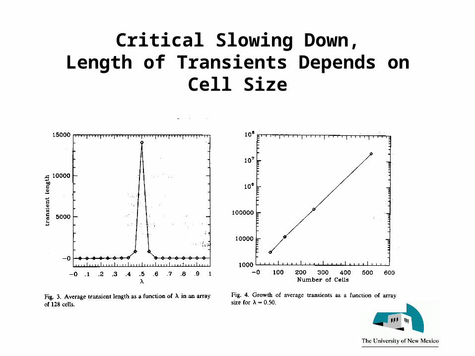
Critical Slowing Down,Length of Transients Depends on Cell Size

Phase Transitions and Lambda

Computation in Cellular Automata
• CA s as computers:– Initial configuration constitutes the data that the physical computer is processing.– Transition function implements the algorithm which is applied to the data. – Examples: Majority calculations, synchronization (Mitchell and Crutchfield).
• CA s as logical universes within which computers can be embedded:– Initial configuration constitutes a computer.– Transition function is the “physics” obeyed by the parts of the embedded computer.– The algorithm and data are functions of the precise state of the initial configuration of
the embedded computer.– In the most general case, the initial configuration is a universal computer. – Examples: Rule 110, Game of life
• CA s can implement storage, counting, logical operators
• CA s are networks of FSAs• A Turing machine is equivalent to an FSA with an infinite storage tape

Example One-Dimensional CARule 110
• The number of states, k=2.• The alphabet • The size of the array, N=11.• The configuration space
• The radius r = 1.• The rule table :
– neighborhood : 000 001 010 011 100 101 110 111– : 0 1 1 1 0 1 1 0
• This is rule 110 (base 10) because the output states are: 01101110 (base 2). Read right to left. Known as Wolfram notation.
• Rule 110 supports universal computation.
),...}11,0,0,0,0,0,0,0,0,0,0(),0,0,0,0,0,0,0,0,0,0,0{(=ΣN
φ
) ( 1it
its φ=+
k=Σ=Σ }1,0{

Rule 110 Space-Time Plot

Two-Dimensional Cellular AutomataSource: Wikipedia
Wire World
Conus textile
Cyclic Cellular Automaton

The Game of Life
• The number of states, k=2.• The alphabet,
– Call 0 “dead” and 1 “alive.”
• The Moore neighborhood:
• Transition rules:– Loneliness: If a live cell has less than 2 live neighbors, then it dies.– Overcrowding: If a live cell has more than 3 live neighbors, then it dies.– Birth: If an empty (dead) cell has 3 live neighbors, then it becomes alive.– Otherwise: If a cell has 2 or 3 live neighbors, then it remains unchanged.
}1,0{=Σ
NE
SW S SE
EW
NNW

Moore vs. Von Neumann Neighborhoods
NE
SW S SE
EW
NNW
S
EW
N
Moore Von Neumann

Example Transition
• Center square changes to one (birth).• “Just 3 for birth, 2 or 3 for survival.”
0
0 1 0
10
10
0 1

Possible Life Histories(Dynamical behaviors that enable universal
computation)
• Static structures:– Beehive, Loaf, Pond, etc. (Figure 15.11)
• Periodic structures:– Blinkers (Figure 15.12)
• Moving structures:– Gliders (next slide)
• Glider guns• Logical gates (and, or, not)• Self-reproducing structures.

Static Objects

Periodic Objects

Gliders (Moving Objects)

Logical Operators

Can we predict the dynamics of a given initial condition?
• Consider a straight line of n live cells:– n = 1,2 Dies out immediately.– n = 3 Blinker– n = 4 Becomes a beehive – n = 5 Traffic lights– n = 6 Dies out at t = 12– n = 7 Interesting behavior, terminating in the honey farm.– N = 8 4 blocks and 4 beehives. – N = 9 2 sets of traffic lights.– Etc.

Reading for Monday
• Wolfram A new kind of science, chapter 11, p 674-691Rule 110 online book at http://www.wolframscience.com/nksonline/toc.html pdf will be posted on course sitehttp://cs.unm.edu/~melaniem/courses/CAS08.html
• Background on tag systems (not required)in Wolfram Chapter 3 and http://mathworld.wolfram.com/CyclicTagSystem.htmlhttp://mathworld.wolfram.com/TagSystem.html
Flake’s applets, C code also downloadablehttp://mitpress.mit.edu/books/FLAOH/cbnhtml/javalarge.html


