Cellular Image Segmentation using N-agent Cooperative … · Cellular Image Segmentation using...

Cellular Image Segmentation usingN-agent Cooperative Game Theory

by

Ian B. Dimock

A research paperpresented to the University of Waterloo

in partial fulfillment of therequirement for the degree of

Master of Mathematicsin

Computational Mathematics

Supervisor: Prof. Justin W.L. Wan

Waterloo, Ontario, Canada, 2015

c© Ian B. Dimock 2015

I hereby declare that I am the sole author of this report. This is a true copy of the report,including any required final revisions, as accepted by my examiners.

I understand that my report may be made electronically available to the public.

ii

Abstract

Image segmentation is an important problem in computer vision and has significant ap-plications in the segmentation of cellular images. Many different imaging techniques existand produce a variety of image properties which pose difficulties to image segmentationroutines. Bright-field images are particularly challenging because of the non-uniform shapeof the cells, the low contrast between cells and background, and imaging artifacts such ashalos and broken edges. Classical segmentation techniques often produce poor results onthese challenging images. Previous attempts at bright-field imaging are often limited inscope to the images that they segment. In this paper, we introduce a new algorithm forautomatically segmenting cellular images. The algorithm incorporates two game theoreticmodels which allow each pixel to act as an independent agent with the goal of selecting theirbest labelling strategy. In the non-cooperative model, the pixels choose strategies greedilybased only on local information. In the cooperative model, the pixels can form coalitions,which select labelling strategies that benefit the entire group. Combining these two modelsproduces a method which allows the pixels to balance both local and global informationwhen selecting their label. With the addition of k-means and active contour techniquesfor initialization and post-processing purposes, we achieve a robust segmentation routine.The algorithm is applied to several cell image datasets including bright-field images, fluo-rescent images and simulated images. Experiments show that the algorithm produces goodsegmentation results across the variety of datasets which differ in cell density, cell shape,contrast, and noise levels.

iii

Acknowledgements

I would like to thank my graduate supervisor Prof. Justin W. L. Wan for all his help inwriting this report. The quality of this work is a testament to his input and guidance. Iwould also like to thank Prof. Kate Larson for taking the time to read this paper.

iv

Dedication

I would like to dedicate this my friends and loved ones. Your support and encouragementhelped make this all possible.

v

Table of Contents

List of Tables viii

List of Figures ix

List of Algorithms xi

1 Introduction 1

1.1 Cellular Images . . . . . . . . . . . . . . . . . . . . . . . . . . . . . . . . . 1

1.1.1 Fluorescent Imaging . . . . . . . . . . . . . . . . . . . . . . . . . . 1

1.1.2 Bright-Field Imaging . . . . . . . . . . . . . . . . . . . . . . . . . . 2

1.2 Image Segmentation . . . . . . . . . . . . . . . . . . . . . . . . . . . . . . 2

1.3 Cellular Image Segmentation . . . . . . . . . . . . . . . . . . . . . . . . . . 3

2 Background 4

2.1 Classical Image Segmentation Algorithms . . . . . . . . . . . . . . . . . . . 4

2.2 Game Theory . . . . . . . . . . . . . . . . . . . . . . . . . . . . . . . . . . 5

2.3 K-means . . . . . . . . . . . . . . . . . . . . . . . . . . . . . . . . . . . . . 6

vi

2.4 Chan-Vese Active Contours . . . . . . . . . . . . . . . . . . . . . . . . . . 7

2.5 ISBI 2013 Cell Tracking Challenge . . . . . . . . . . . . . . . . . . . . . . 9

2.5.1 Datasets . . . . . . . . . . . . . . . . . . . . . . . . . . . . . . . . . 9

2.5.2 Submissions . . . . . . . . . . . . . . . . . . . . . . . . . . . . . . . 11

3 Methodology 13

3.1 N-agent Game Theoretic Image Segmentation . . . . . . . . . . . . . . . . 14

3.1.1 Game Theoretic Objective Function . . . . . . . . . . . . . . . . . . 14

3.1.2 Non-Cooperative Strategy . . . . . . . . . . . . . . . . . . . . . . . 17

3.1.3 Cooperative Strategy . . . . . . . . . . . . . . . . . . . . . . . . . . 19

3.1.4 Strategy Integration . . . . . . . . . . . . . . . . . . . . . . . . . . 21

3.2 Segmentation initialization using two class k-means . . . . . . . . . . . . . 24

3.3 Coalition initialization . . . . . . . . . . . . . . . . . . . . . . . . . . . . . 25

3.4 Smoothing using Chan-Vese Active Contours . . . . . . . . . . . . . . . . . 26

3.4.1 Initialization . . . . . . . . . . . . . . . . . . . . . . . . . . . . . . . 26

3.4.2 Smoothing Procedure . . . . . . . . . . . . . . . . . . . . . . . . . . 27

4 Numerical Results 29

4.1 Bright-Field Images . . . . . . . . . . . . . . . . . . . . . . . . . . . . . . . 30

4.2 ISBI 2013 Cell Tracking Challeng Datasets . . . . . . . . . . . . . . . . . . 33

4.2.1 Jaccard Similarity Index . . . . . . . . . . . . . . . . . . . . . . . . 33

4.2.2 Results . . . . . . . . . . . . . . . . . . . . . . . . . . . . . . . . . . 33

5 Conclusions 48

References 50

vii

List of Tables

4.1 Bright-field segmentation times . . . . . . . . . . . . . . . . . . . . . . . . 32

4.2 Segmentation scores for ISBI 2013 Cell Tracking Challenge . . . . . . . . . 34

viii

List of Figures

1.1 Comparison between fluorescent and bright-field images . . . . . . . . . . . 2

2.1 Sample frames from ISBI 2D videos . . . . . . . . . . . . . . . . . . . . . . 11

3.1 K-means output for bright-field image . . . . . . . . . . . . . . . . . . . . . 25

3.2 Initial cooperative segmentation on bright-field image . . . . . . . . . . . . 26

3.3 Initialization of φ for Chan-Vese . . . . . . . . . . . . . . . . . . . . . . . . 27

3.4 Sample output from the smoothing procedure using active-contours. . . . . 28

4.1 Bright-field image segmentation, large β . . . . . . . . . . . . . . . . . . . 30

4.2 Bright-field image segmentation, small β . . . . . . . . . . . . . . . . . . . 31

4.3 Isolated cell segmentation: 256× 256 . . . . . . . . . . . . . . . . . . . . . 32

4.4 Isolated cell segmentation: 128× 128 . . . . . . . . . . . . . . . . . . . . . 32

4.5 Segmentation of C2DL-MSC - Series 01 . . . . . . . . . . . . . . . . . . . . 36

4.6 Segmentation of C2DL-MSC - Series 01 . . . . . . . . . . . . . . . . . . . . 37

4.7 Segmentation of N2DH-GOWT1 - Series 01 . . . . . . . . . . . . . . . . . 38

4.8 Segmentation of N2DH-GOWT1 - Series 02 . . . . . . . . . . . . . . . . . 39

ix

4.9 Segmentation of N2DL-HeLa - Series 01 . . . . . . . . . . . . . . . . . . . 40

4.10 Segmentation of N2DL-HeLa - Series 02 . . . . . . . . . . . . . . . . . . . 41

4.11 Segmentation of N2DH-SIM - Series 01 . . . . . . . . . . . . . . . . . . . . 42






x

List of Algorithms

3.1 Non-Cooperative Segmentation . . . . . . . . . . . . . . . . . . . . . . . . 18

3.2 Cooperative Segmentation . . . . . . . . . . . . . . . . . . . . . . . . . . . 20

3.3 Combine Non-Cooperative and Cooperative Segmentations . . . . . . . . . 21

3.4 Coalition Reformation . . . . . . . . . . . . . . . . . . . . . . . . . . . . . 22

3.5 Game Theoretic Segmentation . . . . . . . . . . . . . . . . . . . . . . . . . 23

xi

Chapter 1

Introduction

1.1 Cellular Images

In biological science there is often a need to analyse cell images produced by microscopes.Common tasks include counting the number of cells or detecting events such as cell splitting.The analysis of these images can be done by a human or by a computer. Whether theanalysis of a cellular image is to be done by hand or automatically, the type of imagingused plays an important role in the ease of the task. Two general imaging techniques areused: fluorescent and bright-field imaging. Sample fluorescent and bright-field images ofthe same cells can be seen in Figure 1.1.

1.1.1 Fluorescent Imaging

To take a fluorescent image, the cells must first be stained. These stains can target differentparts of the cell such as the nucleus or cytoplasm. When the stained cell is exposedto a specific wavelength of light, it fluoresces at another wavelength. Only the stainedparts of the cell fluoresces, and so they are easily distinguishable from the background.This high contrast is highly desirable for analysing cellular images. There are howeversome drawbacks to fluorescent imaging techniques. Firstly, when using many stains therecan be conflicts between the wavelengths emitted by the microscope and the wavelengthsfluoresced by the cells. There is also the problem of phototoxicity, which is a degradationof the stained cells with repeated exposure to the light used in the fluorescent imaging [22].

1

1.1.2 Bright-Field Imaging

Another type of imaging is called bright-field imaging. In this type of imaging, no stainis applied to the cells, which do not fluorescence, but rather are exposed to white light.This eliminates two of the main problems encountered in fluorescent imaging. The maindisadvantage of bright-field imaging is the low contrast between cells and their background,however, inventions such as phase contrast microscopy [28] can greatly increase the contrastavailable in bright-field images. Bright-field images are particularly suitable for imagingliving cells, and so it is desirable to have automatic segmentation algorithms which canovercome the challenging low contrast. Other artifacts present in bright-field images areglowing edges around cells called halos, as well as broken cell edges.

(a) Fluorescent Image (b) Bright-field Image

Figure 1.1: Fluorescent and bright-field images of the same cells

1.2 Image Segmentation

The problem of image segmentation is a well studied problem in computer vision. The goalis to take an image and automatically divide elements of the image into groups. Thesegroups could be simple like foreground and background, or more complicated, such asidentifying an apple and an orange in an image of a fruit basket. In this report we focus

2

on the segmentation of cellular images. The objective for cellular images is to identify thecells from the background medium in which they are suspended.

There are two general ways to view the problem of image segmentation. If we think ofan image as a grid of pixels, then the segmentation of that image is simply a labelling ofthe pixels as either belonging to the foreground or the background. This will implicitlydefine regions and boundaries in the image. This is the setting in which we develop thegame theoretic segmentation algorithm in Section 3.1. Another equally valid way to viewthe segmentation problem is to find the boundary between foreground and backgroundcomponents. This method will provide implicitly defined labels for each pixel. This set-ting is how the Chan-Vese active contours method is developed in Section 2.4. The twoviewpoints often have subtly different ways of presenting segmentation algorithms, and sokeeping the correct context in mind is important when examining different methods.

1.3 Cellular Image Segmentation

There has been significant research into the area of cellular image segmentation. Mostof this work has been done with fluorescent microscopy, however there has been workdone with bright-field images as well. Tscherepanow et al. propose a mehtod using activecontour methods for bright-field image segmentation [25]. The method performs well, butis applied to only one type of cell and so questions about its robustness remain. A differentalgorithm proposed by Bradbury and Wan uses a spectral k-means method [2] for bright-field image segmentation. This algorithm was also only tested with one series of images.A different approach proposed by Selinummi et al. combines multiple bright-field imagesof the same cells into a higher contrast projection [22]. The method is successful howeverrequires a specific imaging technique to be used. A common problem in most cases is thatthe method tests only on a single dataset. The methods may not be robust for all thevarious issues that arise in different image datasets.

The goal for this work is to provide a cell segmentation routine that performs well onbright-field images as well as datasets from other imaging techniques. The method willideally have minimal parameter tuning which would allow it to perform well on datasetsnot considered. The method uses a game theoretic approach not often used in imagesegmentation. Chapter 2 will introduce some mathematical background needed to developthe segmentation routine, which is presented in Chapter 3. Finally, we present somenumerical results in Chapter 4 and some conclusions in Chapter 5.

3

Chapter 2

Background

2.1 Classical Image Segmentation Algorithms

Image segmentation is an old and important problem in computer vision, and as such, therehave been many algorithms developed over the years. In the rest of this section we discussa few of the classical image segmentation techniques. All three methods discussed behavequite differently, which gives an intuition into the many possible ways to approach theimage segmentation problem. In all cases we consider the binary segmentation problem,which is the problem of segmenting an image into two classes.

The first method we will discuss is that of thresholding. In the thresholding method wesimply compare the intensity of each pixel in the image with some constant threshold value.If the pixels are greater than the threshold they will receive a label of 1 and if not, thenthey will receive a label of 0. This is one of the simplest segmentation techniques, but isoften used as a foundation for more complicated algorithms. The most obvious extensionis to find a way to automatically select the threshold value [18, 21].

Another common classical technique for image segmentation is that of active contours orsnakes. This technique is a form of edge detection. The goal is to find edges in an image,which then represent the boundary between the components we would like to segment.A common approach is to have this active contour be attracted to regions with largegradients in the image. This means the boundary will move to regions in the image withsharp changes in pixel intensity which represent edges. Once the active contour has settled,

4

a segmentation can be recovered by considering the inside and outside of the curve. Beyondthe gradient, many different types of information can be used to dictate the behaviour ofthe contour, leading to many algorithms [3, 5, 11].

The final classical technique we will discuss is that of region growing. In this method,initial seed pixels are selected in the image. From these seeds, neighbouring pixels areconsidered. If a neighbouring pixel is deemed a good enough fit, it is incorporated into thegrouping around that seed pixel. In this way, regions grow out from the seeds until theyrun into each other and every pixel in the image belongs to a group. The determinationof whether a pixel will join a region or not can be done in many different ways as well asthe selection of the initial seeds, all of which lead to a wide variety of algorithms based onthis concept [1, 10, 29].

The method we present in this paper will involve yet a different model. We will presenta segmentation algorithm based on game theory. Game theory can be used in a numberof different ways for segmentation [4, 8, 27], however is not a very common technique forsegmentation purposes. In Section 2.2 we will introduce the necessary components of gametheory before presenting the algorithm in Chapter 3.

2.2 Game Theory

The basic elements of game theory are fairly simple concepts. First is the notion of a game.A game is simply a set of rules within which a number of players act. These players, calledagents, are trying to achieve the best possible reward for themselves within the rules of thegame. The reward for an agent is described by an objective function. An agent typicallyhas a specific set of actions they can perform. The objective function provides a pay-offfor the agent based on his action and the actions of the other players. Game theory isthe study of these games, and is concerned with predicting the outcomes while makingassumptions about the behaviour of the agents.

Games can be broken down and studied in many different ways. We will introduce here avery broad classification of games that will be important in the description of our algorithm.This is the distinction between a cooperative game, and a non-cooperative game. In a non-cooperative game the agents act self-interestedly. This means that the agents care onlyabout maximizing their objective value and are not concerned with the objective values ofthe other agents. To understand the outcome of such games, game theorists often considerthe concept of a Nash Equilibrium [17].

5

A Nash Equilibrium in a game is a set of strategies for all agents in the game such that noagent would improve their objective value by taking a different strategy. In this contexta strategy represents a distribution over the actions available to an agent. A Nash Equi-librium defines strategies for rational agents in that to maximize ones objective value anagent playing a game with other rational agents should play the strategy dictated by theNash Equilibrium. John Nashed proved that in a finite game with rational agents playingstrategies which are distributions over actions, a Nash Equilibrium is guaranteed to exist,although the proof is non-constructive. In practice, Nash Equilibria can be difficult to find.

The Nash Equilibrium for a game can often be unintuitive. The classic example is of thisis the Prisoner’s Dilemma [16]. In this game, the Nash Equilibrium represents an outcomewhere two prisoners betray one another and end up both serving longer sentences than ifboth had stayed silent. If both prisoners had kept quiet, they would both have received alesser sentence than that identified as the Nash Equilibrium. The reason why this happensis because the agents are acting only for themselves, regardless of the other prisonersdecision, confessing will improve a prisoners objective value. Had they been cooperating,the agents would have chosen to both stay silent. Allowing cooperation leads to a newparadigm in game theory, which is the study of cooperative games.

In a cooperative game, the agents are allowed some form of cooperation. The type of coop-eration allowed can be quite varied. One common form of cooperative game allows agentsto form coalitions. By acting together in a coalition, the agents can often improve theirobjective values over what they would have achieved playing self-interestedly. Determininghow agents will form coalitions is another area of study within game theory named thecoalition structure generation problem.

2.3 K-means

The k-means algorithm [13] is a clustering method used to group a sequence of n vectors,(z1, z2, . . . zn) into k distinct classes S = (S1, S2, . . . Sk), where each vector is zi is presentin one and only one class Sj. To split the vectors, the k-means algorithm attempts tominimize the within-cluster sum of squares according to the following formula:

arg minS

k∑i=1

∑z∈Si

‖z − µi‖2, (2.1)

6

where µi is the within cluster mean:

µi =1

|Si|∑z∈Si

z. (2.2)

This is a hard optimization in general, and so the k-means algorithm does not guaranteean optimal solution. The k-means algorithm is initialized by picking k starting centres.These are the vectors µ1, . . . ,µk that will be compared with our input vectors. These canbe chosen a number of ways, one of which is to randomly select k of the input vectors tobecome the centres.

The algorithm then proceeds by alternating two steps: the assignment step, and the updatestep [12]. In the assignment step, each input vector zi is compared to each centre µj.Each vector is then assigned to whichever class had the centre with which it had the leastEuclidean distance. After the assignment step, we proceed with the update step. In theupdate step, the new centres µ are computed using equation (2.2).

The k-means algorithm iterates until no more changes are made in an assignment step.The result is a clustering of the n vectors into k classes.

2.4 Chan-Vese Active Contours

The active contours method of Chan and Vese [5, 24] is an active contours segmentationalgorithm. The algorithm attempts to find a deformable boundary between foreground andbackground components. This is a different way to view the segmentation problem thanthe labelling of pixels we will use to describe the main algorithm in Chapter 3, howeverthey are interchangeable. We introduce this model as it is used as a post-processing stepin the main algorithm.

The algorithm uses a deformable curve, D, defined by the zero level set of a function φ,D = {(x, y) | φ(x, y) = 0}. This curve represents a segmentation; all pixels (i, j) inside thecurve will have φi,j < 0, and all pixels outside the curve will have φi,j > 0. To find φ, thealgorithm solves the following optimization problem:

arg minµ0,µ1,D

F (µ0, µ1, D), (2.3)

7

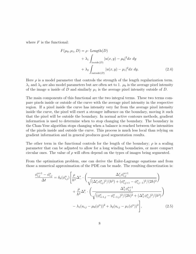
where F is the functional:

F (µ0, µ1, D) = ρ · Length(D)

+ λ1

∫inside(D)

|u(x, y)− µ0|2dx dy

+ λ2

∫outside(D)

|u(x, y)− µ1|2dx dy. (2.4)

Here ρ is a model parameter that controls the strength of the length regularization term.λ1 and λ2 are also model parameters but are often set to 1. µ0 is the average pixel intensityof the image u inside of D and similarly µ1 is the average pixel intensity outside of D.

The main components of this functional are the two integral terms. These two terms com-pare pixels inside or outside of the curve with the average pixel intensity in the respectiveregion. If a pixel inside the curve has intensity very far from the average pixel intensityinside the curve, the pixel will exert a stronger influence on the boundary, moving it suchthat the pixel will be outside the boundary. In normal active contours methods, gradientinformation is used to determine when to stop changing the boundary. The boundary inthe Chan-Vese algorithm stops changing when a balance is reached between the intensitiesof the pixels inside and outside the curve. This process is much less local than relying ongradient information and in general produces good segmentation results.

The other term in the functional controls for the length of the boundary; ρ is a scalingparameter that can be adjusted to allow for a long winding boundaries, or more compactcircular ones. The value of ρ will often depend on the types of images being segmented.

From the optimization problem, one can derive the Euler-Lagrange equations and fromthose a numerical approximation of the PDE can be made. The resulting discretization is:

φn+1i,j − φni,j

∆t= δh(φ

ni,j)

[ρ

h2∆x− ·(

∆x+φ

n+1i,j√

(∆x+φ

ni,j)

2/(h2) + (φni,j+1 − φni,j−1)2/(2h)2

)

+ρ

h2∆y− ·(

∆y+φ

n+1i,j√

(φni+1,j − φni−1,j)2/(2h)2 + (∆y+φ

ni,j)

2/(h2)

)

− λ1(ui,j − µ0(φn))2 + λ2(ui,j − µ1(φ

n))2

], (2.5)

8

where h is the space step, δh is a regularization of the Dirac delta function, and ∆x+,∆

x−,∆

y+,

and ∆y− are forward and backward differences in the x and y directions respectively. An

artificial time step ∆t is also introduced. The function δh is defined as follows:

δh(z) =1

z2 + 1. (2.6)

This function is used to ensure that φ changes only near the boundary (the zero level setof φ). The four finite difference operators are defined as follows:

∆x+φi,j = φi+1,j − φi,j, (2.7)

∆x−φi,j = φi,j − φi−1,j, (2.8)

∆y+φi,j = φi,j+1 − φi,j, (2.9)

∆y−φi,j = φi,j − φi,j−1. (2.10)

We can solve this implicit discretization by alternatingly solving for φn+1, and updatingµ0 and µ1. We stop the iterations after a maximum of T steps or if φ has sufficientlyconverged.

2.5 ISBI 2013 Cell Tracking Challenge

The IEEE International Symposium on Biomedical Imaging 2013 Cell Tracking Challenge1

was held to establish methods for evaluating different automatic cell tracking algorithms[15]. There were eight different datasets used in the competition and six competing al-gorithms. As part of the evaluation, segmentation quality was measured. It is this seg-mentation quality we wish to use when evaluating our algorithm described in Chapter3.

2.5.1 Datasets

The eight datasets can be divided into real videos and simulated videos, and also 2D and3D videos. The real videos are obtained from a variety of imaging techniques. Our efforts

1Challenge website: http://www.codesolorzano.com/celltrackingchallenge/Cell_Tracking_

Challenge/Results_First_CTC.html

9

http://www.codesolorzano.com/celltrackingchallenge/Cell_Tracking_Challenge/Results_First_CTC.html


focus only on the 2D images. For each dataset, a number of ground truths are provided.Due to the high number of frames and cells, however not all cells or frames have groundtruths provided. At least one frame in each dataset is guaranteed to be fully segmented,while cells in other frames are chosen randomly to be given labels in the ground truth.Considering only the 2D videos, we are left with four datasets which are described below.Sample frames are shown in Figure 2.1.

C2DL-MSC

One of the real video datasets. The cells are rat mesenchymal stem cells. The videoconsists of 2D images taken at low resolution using cytoplasmic labelling. Two differenttime series are given for this cell type, having sizes 992× 832 and 1200× 782 respectively.Segmentation challenges include a high signal-to-noise ratio and cells often having longprotrusions.

N2DH-GOWT1

One of the real video datasets. The cells are GOWT1 mouse embryonic stem cells. Thevideo consists of 2D images taken at high resolution using nuclear labelling. Two differ-ent time series are given for this cell type, both having size 1024 × 1024. Segmentationchallenges include variations in staining intensity and cell splitting.

N2DL-HeLa

One of the real video datasets. The cells are histone 2B expressing HeLa cells. The videoconsists of 2D images taken at low resolution using nuclear labelling. Two different timeseries are given for this cell type, both having size 1100 × 700. Segmentation challengesinclude the large number of cells and frequent cell splitting in the images.

N2DH-SIM

One of the simulated video datasets. The simulated videos are generated using a simulationtoolkit [23]. Six different time series are given for this cell type, the largest of which hassize 510 × 580. The variations amongst the simulations provide different challenges tosegmentation, including different noise levels and cell densities.

10

(a) C2DL-MSC (b) N2DH-GOWT1

(c) N2DL-HeLa (d) N2DH-SIM

Figure 2.1: Sample frames from ISBI 2D videos

2.5.2 Submissions

Six groups submitted algorithms to the cell tracking challenge. Below we briefly describethe segmentation algorithm used by each.

COM-US

Segmentation is performed by first computing an intensity histogram. It proceeds byiteratively computing a best-fit N-point histogram. The middle value of this N-pointhistogram provides a threshold for segmentation [6].

11

HEID-GE

Before segmentation a Gaussian filter is applied. Next an initial segmentation was achievedusing adaptive region thresholding. Finally the segmentation is cleaned up using medianfiltering and hole filling [9].

KTH-SE

A smoothed image and a background estimation are produced by convolving two differentGaussian kernels with the original image. After a band pass filter with these two newimages a global thresholding is done to produce a segmentation [14].

LEID-NL

In this algorithm segmentation and tracking are performed simultaneously. At each timestep each cell is fit with a model which evolves over time. The models are fit by performinggradient descent on an energy functional encapsulating different image data [7].

PRAG-CZ

The image is first smoothed by Gaussian filter. Segmentation is performed using an iter-ative thresholding based on k-means. Thresholding is computed on a sliding window tocorrect for differences in different parts of the image [19].

UPM-ES

This algorithm uses spatio-temporal filtering followed by label clustering based on his-togram analysis [20].

12

Chapter 3

Methodology

The segmentation of cellular images presents various challenges that classical segmentationtechniques often fail to overcome. Two challenges in particular are the low contrast be-tween foreground and background pixels as well as the noise introduced by the microscopicimaging techniques. For these reasons, novel approaches are required to effectively segmentcellular images.

In this chapter we outline the algorithm we use to perform cellular image segmentation.We frame the segmentation problem as a game theoretic one, with each pixel in the imageacting as an agent. For cellular image segmentation we are required to divide the imageinto foreground and background - the cells, and the medium in which they are situated.The pixels acting as agents must choose between two strategies representing the foregroundand background. When all agents have reached a consensus on their respective strategies,we are left with our final segmentation.

The game theoretic portion of the algorithm is detailed in Section 3.1. It is based on workby Guo, Yu and Ma [8]. It consists of a non-cooperative component described in Section3.1.2, as well as a cooperative component described in Section 3.1.3. In the non-cooperativegame, agents act self-interestedly and rely only on local information to make their decisions.In the cooperative game, agents are allowed to form coalitions. By acting together in acoalition, agents can improve the coalition-wide results to the detriment of certain agents.By coming to a consensus as a coalition the agents are acting upon information from amuch larger portion of the image than in the non-cooperative game.

13

The algorithm proceeds by combining the results of the cooperative and non-cooperativecomponents. This is possible because in both games, the agents use objective functionsbuilt on the same underlying energy minimization problem described in Section 3.1.1. Theintegration of the components is described in Section 3.1.4.

Additional components are discussed in subsequent sections. The initial splitting of fore-ground and background components using k-means is described in Section 3.2, and theinitial configuration of coalitions is described in Section 3.3. Finally in section Section 3.4we describe a smoothing procedure which uses a Chan-Vese active contours model on thebinary image that is the output of the game theoretic segmentation routine.

3.1 N-agent Game Theoretic Image Segmentation

In this model we represent the m × n pixel image as a 2D grid of points. We index thepoints either by a conventional pair (i, j), with i ∈ {1 . . .m}, j ∈ {1 . . . n} or as a singleindex s ∈ S = {1 . . . N} where N = m · n. We can convert from (i, j) to s using thefollowing formula:

s = m · (j − 1) + i. (3.1)

The image data is given as u = (u1, . . . , uN), where each us takes a value between 0 and1, representing the intensity of a pixel. The goal of image segmentation is to identifyforeground and background components. To achieve this we would like to assign each pixelin the image to either the background or the foreground represented by a label 0 or 1. Werepresent the segmentation as w = (w1, . . . , wN), here each ws is a binary variable takingeither 0 or 1. A segmentation w thus provides each pixel with a label giving us potentialforeground and background components.

3.1.1 Game Theoretic Objective Function

There are 2N possible segmentations of a given image with N pixels. We would liketo find the best possible segmentation of our image. We call this optimal segmentationw∗. The segmentation w∗ is that segmentation which is best explained by the pixelsin our image. We can write this as a conditional probability P (w|u). This probabilityrepresents the quality at which a given segmentation w is explained by the image u. Finding

14

the segmentation w∗ which maximizes this probability is an optimization problem withobjective function P (w|u). By applying Bayes’ rule we arrive at the following optimizationproblem:

w∗ = arg maxw

P (w|u) = arg maxw

P (u|w)P (w). (3.2)

Under the random field model we are using, we have that P (u|w) is independent across allpoints in the grid, so:

P (u|w) =∏s

P (us|ws). (3.3)

We further assume that the distribution of P (us|ws) is Gaussian. We have two classes,foreground and background, represented by 0 and 1. Each class will be represented byits own Gaussian distribution. We specify these distributions by means and standarddeviations: (µ0, σ0) for class 0, and (µ1, σ1) for class 1. We will let k represent one of thetwo possible labels for a pixel, 0 or 1, so k ∈ {0, 1}. We are now ready to write down thedistribution for P (us|ws) for a pixel s taking class k:

P (us|ws) =1√

2πσkexp

(−(us − µk)2

2σ2k

). (3.4)

To simplify our optimization we take the log of the argument. This preserves optimalitysince log is a monotone function. We get:

w∗ = arg maxw

∑s

[log (P (us|ws))

]+ log (P (w)) . (3.5)

The 2D grid that we have presented with the Gaussian distribution is a Markov RandomField (MRF). It satisfies the conditions of the Hammersley-Clifford Theorem, which allowsus to write P (w) according to a Gibbs distribution:

P (w) =1

Zexp

(−∑X∈X

V X(w)

). (3.6)

Here, Z is called the normalizing constant, and can be ignored after taking the logarithm.The function V X is called the clique potential for a clique X. A clique is a set of pixels allof which neighbour each other. We consider only four neighbours for each pixel (up, down,left, and right) so cliques in our grid consist only of pairs of pixels. Here X represents the

15

set of all cliques. We consider four neighbours for each pixel which produces only cliquesof size two. This is because all pixels in a clique must be neighbours with one another.Since we only ever consider cliques of size two, we can redefine the potential functioncorrespondingly:

V X(w) ≡ v(ws, wr) =

{−β if ws = wr

β if ws 6= wr,where X = {s, r}. (3.7)

Here β is a model parameter, which controls the scaling of the clique potential.

We can express our optimization in terms of energy. We wish to find the lowest totalenergy Etot. We express this by expanding P (w) in our objective function and groupingall terms by index s to get:

w∗ = arg minw

Etot ≡ arg minw

∑s

E(u,w, s), (3.8)

where E(u,w, s) represents the local energy for a given pixel s. It is the combination ofterms from the Gaussian distribution and the clique potentials of all cliques to which sbelongs. Recall, a pixel can be labelled 0 or 1 in our segmentation w. We define the energywhen pixel s is labelled 0 to be E0(u,w, s). Similarly, when pixel s is labelled 1 the energyis E1(u,w, s). To minimize the total energy, we define the local energy of each pixel to bethe minimum of these two:

E(u,w, s) = min[E0(u,w, s), E1(u,w, s)

]. (3.9)

The energy E0(u,w, s) is computed using (µ0, σ0) from the Gaussian distribution for class0, and is defined as follows:

E0(u,w, s) = log(√

2πσ0) +(us − µ0)

2

2σ20

+∑r∈N(s)

v(0, wr), (3.10)

where N(s) represents the neighbourhood of pixel s (all pixels belonging to a clique withs). We can similarly define E1(u,w, s):

E1(u,w, s) = log(√

2πσ1) +(us − µ1)

2

2σ21

+∑r∈N(s)

v(1, wr). (3.11)

16

Equations (3.10) and (3.11) give us a way to compare the two possible labels to which wecan assign to pixel s. They will be the foundation on which we build the cooperative andnon-cooperative components described in the following sections.

3.1.2 Non-Cooperative Strategy

From an initial segmentation w0, we allow the pixels (agents) to compete in a non-competitive game where each pixel tries to minimize its local energy, using the labelsof its neighbours as information. By finding a Nash equilibrium amongst the agents wecan achieve the desired result where no agent is able to improve its objective value bychanging its label.

There are two difficulties in finding this equilibrium. Firstly, we are not allowing thepixels to pick strategies which are distributions over their actions, and as such the NashEquilibrium is not guaranteed to exist. Secondly, even if it does exist it may be difficultto find due to the number of agents involved. We turn to a technique called best responsedynamics, which is a method by which agents choose their strategies. It is an iterativeprocedure by which agents update their strategy based on local information. In this case,the pixels will update their label based on the labels of their neighbours. By this we meanthat each pixel s will compute E0 and E1 based on the previous segmentation, and chooseeither the strategy 0 or 1 which produced the lowest energy. This process can converge toa Nash equilibrium or sometimes get stuck in a cycle. Our observations are that if a cycleis encountered it is only with a small portion of the pixels. We can halt the iterations ifthis cycling occurs and the result is sufficient to achieve the desired results.

The general procedure for the non-cooperative game is outlined in Algorithm 3.1. Theinputs for the algorithm are the original image, u, some initial segmentation w0, as wellas a limit on the number of iterations, K, which will be a model parameter. The initialsegmentation comes from the initialization process described in Section 3.2 or from previousiterations of the iterative procedure described in Section 3.1.4.

17

Algorithm 3.1 Non-Cooperative Segmentation

Input: Image u, initial segmentation w0

Output: Segmentation wnon−coop, local energies Enon−coop

1:

2: function Non-Cooperative-Segmentation(u,w0)3: for i = 1 to K do4: Compute µ0, σ0, µ1, σ1 from wi−1 and u5: for Each pixel s ∈ S do6: Compute E0 = E0(u,wi−1, s)7: Compute E1 = E1(u,wi−1, s)8: if E0 < E1 then9: Set wis = 0

10: Set Enon−coops = E0

11: else12: Set wis = 113: Set Enon−coop

s = E1

14: end if15: end for16: if wi = wi−1 then17: return wi, Enon−coop

18: end if19: end for20: return wK , Enon−coop

21: end function

Each iteration i of the algorithm starts by computing the mean and standard deviationfor the two classes 0 and 1. This is done by using the segmentation labels provided by theprevious iteration (or the initial segmentation w0). The algorithm proceeds by computingenergies E0 and E1 for each pixel s using equations (3.10) and (3.11). Finally the algorithmchooses the preferred label wis for each pixel by comparing E0 and E1. It also stores thevalue of the local energy it has chosen in the variable Enon−coop, which is also indexed by S.These local energies and the final segmentation wnon−coop are the outputs of the algorithm.

Segmentation results from this algorithm are generally not very good. In this non-cooperativegame the agents make decisions base only on information from their four neighbouring pix-els. This tends to produce a lot of noise in the final segmentation. We wish to provide away for the pixels to incorporate information into their decisions from further away in the

18

image. In the next section we introduce a cooperative component to the game that allowsthe agents to do just this.

3.1.3 Cooperative Strategy

To introduce cooperation into the game that the agents are playing we first introduce theconcept of a coalition. Here we define a coalition C to be a collection of pixels C ⊆ S,such that all pixels are all spatially connected, meaning all pixels can be reached fromone another by travelling amongst shared neighbours. We can split the entire image intocoalitions in this way. We introduce the collection of all coalitions, C = {C1, C2, . . . , CP},with the properties that the entire image is divided amongst the coalitions, S = C1 ∪C2 ∪. . . ∪ CP , and that no two coalitions share any pixels, Ci ∩ Cj = ∅,∀i 6= j.

We also introduce an extension to the local energy functions from (3.10) and (3.11) todefine energies for an entire coalition:

E0(u,w,C) ≡∑s∈C

E0(u,wC,0, s), (3.12)

E1(u,w,C) ≡∑s∈C

E1(u,wC,1, s). (3.13)

Here we use special segmentations wC,0 and wC,1 as input to the local energy functions;wC,0 is a modification of the segmentation w in which every pixel s ∈ C is re-labelled 0,and similarly wC,1 is a modification of the segmentation w in which every pixel s ∈ C isre-labelled 1.

With a set of coalitions, C, we proceed by allowing each coalition to decide as a groupwhich strategy all pixels belonging to that coalition will take. This procedure is detailedin Algorithm 3.2. Inputs to the algorithm are the image u, an initial segmentation w0, anda set of coalitions C.

19

Algorithm 3.2 Cooperative Segmentation

Input: Image u, initial segmentation w0, coalitions COutput: Segmentation wcoop, local energies Ecoop

1: function Cooperative-Segmentation(u,w0, C)2: Compute µ0, σ0, µ1, σ1 from w0 and u3: for C ∈ C do4: Let wC,0 = wC,1 = w5: Set wC,0s = 0,∀s ∈ C6: Set wC,1s = 1,∀s ∈ C7: Compute E0 =

∑s∈C

E0(u,wC,0, s)

8: Compute E1 =∑s∈C

E1(u,wC,1, s)

9: if E0 < E1 then10: ∀s ∈ C, set wcoops = 011: ∀s ∈ C, set Ecoop

s = E0(u,wC,0, s)12: else13: ∀s ∈ C, set wcoops = 114: ∀s ∈ C, set Ecoop

s = E1(u,wC,1, s)15: end if16: end for17: return wcoop, Ecoop

18: end function

The algorithm begins by computing the means and standard deviations for the classes 0and 1 specified by the initial segmentation w0. It continues by computing coalition energiesfor each C ∈ C. It computes the energy E0 given that the entire coalition C takes label0 using equation (3.12) and the energy E1 given that the entire coalition C takes label1 using equation (3.13). By comparing these two coalition wide energies, the coalitionmakes a decision as to which label all its members should take. It stores the relevant localenergies and also the labels that are chosen by each coalition. We are left at the end withthe cooperative segmentation wcoop and the collection of local energies, Ecoop, which eachpixel computed when choosing its label.

This cooperative game tends to produce large coalitions, and has trouble segmenting finedetails in the image because there is no way to reduce coalition size. To achieve a segmen-tation with strengths from both the the non-cooperative routine as well as this cooperative

20

one, we incorporate the two into a single segmentation algorithm, described in the nextsection.

3.1.4 Strategy Integration

In this section we describe the procedure by which the non-cooperative and cooperativesegmentation routines are integrated into a single procedure. We have segmentations pro-duced by those routines: wnon−coop and wcoop. We also have the collection of local energiescomputed as each pixel chose its label in Algorithms 3.1 and 3.2: Enon−coop and Ecoop.

Normally two segmentations would be hard to compare and combine, however we built eachroutine upon the same local energy functions (3.10) and (3.11). To produce a combinedsegmentation, wcomb, we simply compare the cooperative and non-cooperative energies fromEnon−coop and Ecoop. The details of this are presented in Algorithm 3.3.

Algorithm 3.3 Combine Non-Cooperative and Cooperative Segmentations

Input: Segmentations wnon−coop and wcoop, energies Enon−coop and Ecoop

Output: Segmentation wcomb

1: function Combined-Segmentation(wnon−coop, wcoop, Enon−coop, Ecoop)2: for s ∈ S do3: if Enon−coop

s < Ecoops then

4: Set wcombs = wnon−coops

5: else6: Set wcombs = wcoops

7: end if8: end for9: return wcomb

10: end function

As mentioned, the inputs to the algorithm are the two segmentations and the two collectionsof local energies: wnon−coop, wcoop, Enon−coop, and Ecoop. For each pixel s, the algorithmcompares the local energies Enon−coop

s and Ecoops . Whichever has the smaller energy, provides

the label for the combined segmentation wcomb. In this way each pixel in the combinedsegmentation is provided with a label from wither wnon−coop or wcoop.

21

Similar to the iterations in the non-cooperative component with the intent of converging toa Nash equilibrium, we can iterate this combination procedure until a stable segmentationis reached. At each step we must update the coalitions with information from the newcombined segmentation. To form the new set of coalitions we group all spatially connectedpixels with the same label in wcomb. In this work we consider only maximal coalitions. Thatis coalitions of spatially connected pixels taking the same strategy must be in the samecoalition. This can be done using breadth first search, the details of which are detailed inAlgorithm 3.4.

Algorithm 3.4 Coalition Reformation

Input: Segmentation wOutput: Set of coalitions C

1: function Get-Coalitions(w)2: Initialize C1 = {}3: i = 14: Initialize C = {}5: Initialize Ms = false,∀s ∈ S6: while ∃s, such that Ms = false do7: Find s, such that Ms = false8: Let Q = {s}9: while Q not empty do

10: Let Q = Q \ {s}11: Let Ci = Ci ∪ {s}12: Set Ms = true13: for r ∈ N(s) do14: if ws = wr and Mr = false then15: Let Q = Q ∪ {r}16: end if17: end for18: end while19: Let C = C ∪ Ci20: Let i = i+ 121: Let Ci = {}22: end while23: return C24: end function

22

The breadth first search marks each pixel s as it is found, storing that information in M .The algorithm continues as long as there are unmarked pixels. When an unmarked pixel sis found, a new coalition is formed. The algorithm proceeds by adding all pixels r spatiallyconnected to s that have the same label (ws = wr) to the coalition. All pixels in thiscoalition are then marked and we proceed to look for another unmarked pixel. The endresult is a new set of coalitions C.

With a new set of coalitions we repeat the process of computing both the non-cooperativeand cooperative segmentations, as well as performing the combination procedure. Thesesteps are iterated a certain number of times specified by parameter L. In general, thealgorithm is found to converge in ∼ 10 iterations.

The complete algorithm is presented in Algorithm 3.5. The inputs to the algorithm arean image u, an initial segmentation w0 and an initial set of coalitions C. The procedure ofhow to get w0 and C are discussed in Sections 3.2 and 3.3.

Algorithm 3.5 Game Theoretic Segmentation

Input: Image u, initial segmentation w0, initial coalitions COutput: Segmentation wgt

1: function GT-Segmentation(u,w0, C)2: wgt = w0

3: for i = 1 to L do4: wnon−coop, Enon−coop = Non-Cooperative-Segmentation(u,wgt)5: wcoop, Ecoop = Cooperative-Segmentation(u,wgt, C)6: wgt = Combined-Segmentation(wnon−coop, wcoop, Enon−coop, Ecoop)7: C = Get-Coalitions(wGT )8: end for9: return wgt

10: end function

Each iteration of the algorithm starts by computing (wnon−coop, Enon−coop) using Algorithm3.1 and (wcoop, Ecoop) using Algorithm 3.2. We then produce a combined segmentationwcomb using Algorithm 3.3. The final step is to recompute the coalitions for use in the nextiteration using Algorithm 3.4.

The final game theoretic segmentation wgt produced by this algorithm is found to be quitegood in practice. We will apply some post-processing procedures to eliminate noise that

23

is often present when noisy images are used as input. This process is described in Section3.4. Numerical results and sample segmentations using this algorithm are presented anddiscussed in Chapter 4.

3.2 Segmentation initialization using two class k-means

The game theoretic segmentation presented in Section 3.1 requires an initial segmentationas input. This could be a circle dividing up the image into two groups or some othertrivial division of the pixels. Experiments with several methods of choosing an initialsegmentation showed that the algorithm converges more quickly if the initial segmentationhas some resemblance to the final segmentation.

We use the k-means algorithm described in Section 2.3 for this purpose. We consider onlythe two class k-means algorithm (k = 2) and our input will be the pixel intensities whichare scalars. This gives us a simplified version of equation (2.1). Using the notation fromour image segmentation problem we get the k-means optimization problem:

arg minw

∑s: ws=0

‖us − µ0‖2 +∑

s: ws=1

‖us − µ1‖2. (3.14)

This greatly simplified k-means runs quickly even for a large number of pixels.

The k-means algorithm will divide the pixels into two groups based on intensity. This isgenerally not a good segmentation for low contrast images such as the cellular images weare concerned with, but the k-means algorithm for two classes with scalar inputs is fast,and the result is sufficient for our initialization purposes.

An added benefit is that the k-means algorithm implicitly returns the mean of each classwhich saves that computation from the first iteration of the game theoretic segmenta-tion. K-means is a heuristic algorithm and therefore not guaranteed to converge to theglobal optimum. This is again is acceptable for our purposes as we require only a roughsegmentation to initialize our algorithm.

Figure 3.1 shows an example k-means segmentation used as input to the game theoreticsegmentation.

24

(a) Bright-field cellular image (b) Two class k-means segmentation

Figure 3.1: Two class k-means run on bright-field cellular image pixel intensities.

3.3 Coalition initialization

The cooperative component of the game theoretic segmentation from Section 3.1.3 requiresan a initial set of coalitions C. Using Get-Coalitions from Algorithm 3.4 after the k-means segmentation is one option, however there are a few problems that rule it out. Thecell images we are segmenting are often noisy. This results in a k-means segmentation thatis quite noisy. If we run Get-Coalitions on this segmentation we end up with numerouscoalitions that consist of only a few or even single pixels. These numerous small coalitionscause a lot of work in the cooperative component of the algorithm while at the same timelosing the more global property we desire from our coalitions.

We instead divide the entire image into square blocks of size B × B, which become ourcoalitions. B is a model parameter that must be selected carefully; we balance block sizesbeing too small to give desirable coalition benefits or too large and losing resolution inthe cooperative segmentation resulting from the coalitions. On the first iteration of thegame theoretic algorithm the coalitions will not represent spatially connected pixels withthe same label as they do in the remaining iterations.

Figure 3.2 shows an example cooperative segmentation resulting from these block coali-

25

tions.

(a) Bright-field cellular image (b) Cooperative segmentation using 8× 8block coalitions

Figure 3.2: First iteration for cooperative segmentation on bright-field cellular image.

3.4 Smoothing using Chan-Vese Active Contours

We use the Chan-Vese active contours method described in Section 2.4 as a post-processingstep after the game theoretic segmentation algorithm. The game theoretic algorithm canoften have a fair amount of noise in the final segmentation, and we use the active contoursmethod to achieve a smoother segmentation. We use the binary output of our gametheoretic segmentation as input to the active contours algorithm.

3.4.1 Initialization

The function φ defining our boundary should be a signed distance function. For a generalimage, Chan-Vese segmentation usually begins with a circle or other simple shape defining

26

the boundary. The signed distance function in this case is easy to define. We howeverwould like to start with the zero level being the boundary defined by the output of thegame theoretic segmentation.

Computing the signed distance for the complicated shapes resulting from the image seg-mentation is challenging. We instead approximate this by computed a signed Manhattandistance on the grid specified by the pixels. This is done by giving interior pixels next tothe boundary a value of 1. Interior pixels that are neighbours to the pixels of value 1 aregiven a value of 2 and so on. The same procedure is done for pixels outside of the boundaryhowever the values are negative. An example of this can be seen in Figure 3.3.

-3 -2 -1 -1 -2 -3 -4-2 -1 1 1 -1 -2 -3-1 1 2 2 1 -1 -2-1 1 2 2 1 -1 -2-1 1 2 3 2 1 -1-1 1 2 2 1 -1 -2-1 1 1 1 -1 -2 -3

Figure 3.3: Example initialization of φ with interior pixels (gray) positive and exteriorpixels (white) negative.

3.4.2 Smoothing Procedure

The active contours algorithm uses several parameters to control the resulting segmenta-tion: ρ, λ1, λ2, h,∆t, T . With these parameters specified, and φ0 initialized as in Section3.4.1, we are ready to begin the algorithm. We solve equation (2.5) for φn+1, and iter-ate until convergence or until we have reached T iterations. Generally ∼ 10 iterations issufficient for our smoothing purposes.

The final output is a significantly smoother version of the segmentation generated fromthe game theoretic algorithm. A comparison of before and after smoothing can be seen inFigure 3.4.

27

(a) Segmentation before smoothing (b) Segmentation after smoothing

Figure 3.4: Sample output from the smoothing procedure using active-contours.

28

Chapter 4

Numerical Results

From Chapter 3 we have a collection of parameters we must specify for the model. Fromthe game theoretic portion we have: B, the block size of the initial coalitions; L, themaximum number of iterations we will perform; β, a parameter in the energy functioncontrolling the tendency to allow noise; and K, the number of iterations allowed in thenon-cooperative component. In all cases we fix L = 10 and K = 30.These values weredeemed sufficient for convergence in every instance tested.

For the smoothing procedure we use the Chan-Vese active contour algorithm which itselfhas a number of parameters: h, the space step size; ∆t, the time step size; λ1, λ2 and ρ,scaling parameters; and T , the maximum number of iterations. In all cases we fix h = 1,∆t = 0.3, λ1, λ2 = 1, and T = 10. The values for h, λ1, and lambda2 are taken fromliterature and the values for ∆t and T were selected from experimentation.

When listing parameters for a given segmentation result only B, β, µ will be specified. Asmall B is often required for images with many small details. The parameter β has the mosteffect on the resulting segmentation; a small β punishes pixels less for choosing strategiesdifferent from their neighbours. Several consequences result from choosing a small β value,we can segment regions of the image that are harder to distinguish from the backgroundbut at the same time it can also lead to over segmentation and more noise in the final result.Large β values swing the trade-off in the other direction, giving less noise and less over-segmentation, but less difficult to segment regions are ignored. The parameter ρ controlsthe smoothness of the result produced by Chan-Vese, in other words how aggressively itwill eliminates noise and sharp corners. This parameter can vary depending on the generalshape of the cells in the images we wish to segment.

29

4.1 Bright-Field Images

The bright-field images used are of C2C12 cells [26]. The result of the two segmentationon the same bright-field image can be seen in Figures 4.1 and 4.2. In Figure 4.1 we havechosen a large value for β, while in Figure 4.2 a smaller β. We can see that the algorithmcaptures most of the cells. Two cells on the right hand side of the image contain somedifficult to capture low contrast regions. The result with smaller β captures more of thedifficult cells but it also over-segments in several locations. Which result is better may bea matter of contention.

Figure 4.1: Bright-field image segmentation using game theoretic algorithm. Top row:original image, segmentation before smoothing. Bottom Row: final segmentation, visual-ization B = 12, β = 2.2, ρ = 6. Image size: 512× 512.

30

Figure 4.2: Bright-field image segmentation using game theoretic algorithm. Top row:original image, segmentation before smoothing. Bottom Row: final segmentation, visual-ization. B = 12, β = 0.6, ρ = 6. Image size: 512× 512.

Improvements can be made if we isolate cells in the image and perform segmentationon them individually. This is not unexpected as the information from other cells couldnegatively influence the segmentation of a specific cell. Figures 4.3 and 4.4 offer twoinstance where an isolated segmentation results in an improved result from the full imagesegmentation.

31

Figure 4.3: Bright-field image segmentation using game theoretic algorithm. Left-to-right:original image, segmentation before smoothing, final segmentation, visualization. B = 6,β = 0.5, ρ = 6. Image size: 256× 256.

Figure 4.4: Bright-field image segmentation using game theoretic algorithm. Left-to-right:original image, segmentation before smoothing, final segmentation, visualization. B = 12,β = 1.2, ρ = 6. Image size: 128× 128.

Some timing results for different image size can be found in Table 4.1. Each step up insize is actually a quadrupling in the number of pixels. We see a roughly ten-fold increasein time taken for the game theoretic algorithm at each size increase and less than that forthe smoothing portion.

Image Size Game Theoretic Time (s) Chan-Vese Time (s)128× 128 1.410101 0.977529256× 256 15.03144 4.95104512× 512 138.67926 34.69564

Table 4.1: Timing results for different size bright-field images

32

4.2 ISBI 2013 Cell Tracking Challeng Datasets

4.2.1 Jaccard Similarity Index

The results published in [15] use a standard measure to compare segmentation results acrossthe different algorithms. We compare our segmentation results so that we can comparethe effectiveness of our algorithms to that of the submitted algorithms described in Section2.5.2.

From an image frame I, a ground truth G was hand labelled. Due to the number of totalcells across all data sets, only a certain number of cells in each frame was labelled, althoughone frame was guaranteed to be fully labelled in each dataset. For each labelled frame then,we compare it to the segmentation produced by our algorithm. For each labelled cell R,we first decide whether there is a corresponding cell in our segmented image. We considereach cell S present in the segmented image and consider them matching if

|R ∩ S| > 0.5 · |R| (4.1)

The size of a cell or its intersection with another cell is simply the number of pixels in thatlabelled cell. After we determine that the cells correspond to one another, we measuretheir similarity using the Jaccard similarity index:

J(R, S) =|R ∩ S||R ∪ S|

(4.2)

We can see that if the segmentation matches the ground truth exactly, R ∩ S = R ∪ Sand so we will have J(R, S) = 1. Likewise, if the segmentation does not match the groundtruth cell will have J(R, S) = 0.

By averaging the Jaccard index across every cell in each frame of a dataset we can producea score between 0 and 1. This give an indication of how successful the segmentationalgorithm is and can be used to compare the effectiveness of different algorithms.

4.2.2 Results

Segmentation results from the IEEE International Symposium on Biomedical Imaging 2013Cell Tracking Challenge compared with our game theoretic algorithm is presented in Table4.2.

33

Dataset C2DL-MSC

N2DH-GOWT1

N2DL-HeLa

N2DH-SIM

Series 01 02 01 02 01 02 01 02 03 04 05 06

COM-US 0.06 0.15 0.69 0.39 0.33 0.3 0.75 0.77 0.65 0.64 0.64 0.75HEID-GE 0.34 0.43 0.84 0.89 0.83 0.8 0.91 0.9 0.82 0.83 0.81 0.89KTH-SE 0.49 0.66 0.86 0.91 0.88 0.89 0.91 0.89 0.84 0.83 0.8 0.83

LEID-NL N/A N/A 0.84 0.88 0.74 N/A 0.93 0.91 0.83 0.84 0.84 0.91PRAG-CZ 0.15 0.21 0.86 0.92 0.78 0.76 0.8 0.8 0.75 0.78 0.76 0.79

UPM-ES 0.41 0.19 0.55 0.63 0.63 0.65 0.91 0.89 0.81 0.82 0.77 0.86GameTheoretic 0.55 0.75 0.86 0.93 0.69 0.73 0.9 0.92 0.84 0.86 0.94 0.89

Table 4.2: Segmentation scores for ISBI 2013 Cell Tracking Challenge as well as gametheoretic algorithm1. Bolded entries are the highest score for that dataset.

There are a number of notable results we can see from the scores. The KTH-SE submissionis one the strongest of the submitted algorithms. It performs the best on all but one of thereal videos and quite well on the simulated videos. The game theoretic algorithm achievesa better segmentation score than the KTH-SE algorithm on nine of the twelve datasets.The LEID-NL submission did not perform well on the real datasets, but had the bestsegmentation for five of the six simulated videos. Comparing our game theoretic algorithmto LEID-NL, we can see that it out performs it on five of the six simulated videos. Fromthese comparisons we can conclude that the game theoretic algorithm we have developed isa good segmentation algorithm, which has out performed two of the strongest submissionsto the ISBI Cell Tracking Challenge.

Of all the datasets from the challenge, the game theoretic algorithm struggled most withthe N2DL-HeLa videos, scoring below several of the submitted algorithms. Sample imagesand segmentations can be seen in Figures 4.9 and 4.10. We can see from these images thatthey contain a large number of densely packed cells. We note in particular that the gametheoretic algorithm has a tendency to over segment (labelling extra background pixels asbelonging to cells near the borders). The over segmentation is especially harmful whenthere are so many densely packed, as the segmentations of neighbouring cells will begin tooverlap. This problem might be addressed with more intensive parameter tuning or mightinvolve a more sophisticated approach to creating coalitions.

The C2DL-MSC datasets provide a different story however. Here we can see big im-

1Adapted from http://www.codesolorzano.com/celltrackingchallenge/Cell_Tracking_

Challenge/Results_First_CTC.html

34



provements in the segmentation score by the game theoretic algorithm over those of thesubmitted algorithms. Many of the submitted algorithms had difficulty segmenting the im-ages from both C2DL-MSC series. The C2DL-MSC datasets are challenging because theycontain whole cells with irregular shapes, whereas many of the other datasets contain moreuniform rounded cell nuclei. Figures 4.5 and 4.6 show sample images and segmentationsfor these datasets.

Sample segmentations for the N2DH-GOWT1 series can be seen in Figures 4.7 and 4.8.Of note for this dataset is the large difference in intensities of certain cells. In Figure 4.7we see a cell near the bottom of the image that was present in the ground truth but notcompletely segmented by our algorithm. Elsewhere in the image we find segmented cellsthat are hard to see even with the human eye.

Sample segmentations for the simulated N2DH-SIM series can be seen in Figures 4.11 to4.16. Of note in these datasets are the bright spots in the cells of Figures 4.15 and 4.16,which lead to low contrast near the borders of the cells.

35

Figure 4.5: Segmentation for C2DL-MSC dataset, series 01. Top row: original image,ground truth. Bottom Row: final segmentation, visualization. B = 16, β = 2.5, ρ = 10.

36

Figure 4.6: Segmentation for C2DL-MSC dataset, series 02. Top row: original image,ground truth. Bottom Row: final segmentation, visualization. B = 16, β = 2.5, ρ = 10.

37

Figure 4.7: Segmentation for N2DH-GOWT1 dataset, series 01. Top row: original image,ground truth. Bottom Row: final segmentation, visualization. B = 25, β = 2.6, ρ = 10.

38

Figure 4.8: Segmentation for N2DH-GOWT1 dataset, series 02. Top row: original image,ground truth. Bottom Row: final segmentation, visualization. B = 16, β = 1.8, ρ = 10.

39

Figure 4.9: Segmentation for N2DL-HeLa dataset, series 01. Top row: original image,ground truth. Bottom Row: final segmentation, visualization. B = 14, β = 2.2, ρ = 10.

40

Figure 4.10: Segmentation for N2DL-HeLa dataset, series 02. Top row: original image,ground truth. Bottom Row: final segmentation, visualization. B = 20, β = 2.0, ρ = 10.

41

Figure 4.11: Segmentation for N2DH-SIM dataset, series 01. Top row: original image,ground truth. Bottom Row: final segmentation, visualization. B = 20, β = 1.2, ρ = 10.

42


43


44


45


46


47

Chapter 5

Conclusions

In this work we developed a novel algorithm to perform segmentation using a combinationof game theoretic models not often used for segmentation purposes and more classicalsegmentation techniques. The game theoretic component combines two paradigms of gametheory, cooperative and non-cooperative games, into a single algorithm. Combined withautomatic initialization using k-means and post-processing using active contours, the resultwas a robust segmentation algorithm that requires minimal parameter tuning.

The algorithm was tested using a set of bright-field images as well as twelve datasets fromthe ISBI 2013 Cell Tracking Challenge. The cell tracking challenge provided twelve 2-dimensional datasets, six of which were simulated and six of which were microscope images.On the bright-field images, the algorithm performed well. The method is able to segmentthe entire frame containing multiple cells. Results were better when the cells are isolated.This suggests that a more localized approach may produce better results when segmentingthe entire frame. For the datasets from the Cell Tracking Challenge, segmentations werecompared using the Jaccard similarity index. This allowed a direct comparison betweenour game theoretic algorithm and the segmentation scores of the algorithms submitted tothe competition. Our algorithm perform well across most datasets in the competition. Thegame theoretic algorithm performed especially well on the challenge dataset C2DL-MSC,which has low contrast and non-uniform cell shapes. This type of image is most similar tothe bright-field images with which we compared, and the most difficult to segment of the2-dimensional datasets provided by the competition.

There are certain areas which might be investigated for future work. The algorithm ingeneral tends to slightly over-segment which causes problems on images such as the N2DL-

48

HeLa dataset from the cell tracking challenge. This dataset has a very high cell densityand the over-segmentation here leads to poor results. Another area of investigation wouldbe in the segmentation of 3-dimensional videos. In this setting the algorithm would besegmenting time-series of 3-dimensional frames. The cell tracking challenge offers datasetsof this nature and these types of videos are becoming more common in cellular imaging.

49

References

[1] R. Adams and L. Bischof, Seeded region growing, IEEE Transactions on PatternAnalysis and Machine Intelligence, 16 (1994), pp. 641–647.

[2] L. Bradbury and J. W. L. Wan, A spectral k-means approach to bright-field cellimage segmentation, in 2010 Annual International Conference of the IEEE Engineer-ing in Medicine and Biology Society (EMBC), IEEE Engineering in Medicine andBiology Society Conference Proceedings, 2010, pp. 4748–4751. 32nd Annual Interna-tional Conference of the IEEE Engineering-in-Medicine-and-Biology-Society (EMBC10), Buenos Aires, Argentina, Aug 30-Sep 04, 2010.

[3] V. Caselles, F. Catte, T. Coll, and F. Dibos, A geometric model for activecontours in image-processing, Numerische Mathematik, 66 (1993), pp. 1–31.

[4] A. Chakraborty and J. S. Duncan, Game-theoretic integration for image seg-mentation, IEEE Transactions on Pattern Analysis and Machine Intelligence, 21(1999), pp. 12–30.

[5] T. F. Chan and L. A. Vese, Active contours without edges, IEEE Transactions onImage Processing, 10 (2001), pp. 266–277.

[6] S. Coraluppi and C. Carthel, Modified scoring in multiple-hypothesis tracking,Journal of Advances in Information Fusion, 7 (2012), pp. 153–164.

[7] O. Dzyubachyk, W. A. van Cappellen, J. Essers, W. J. Niessen, andE. Meijering, Advanced level-set-based vell tracking in time-lapse fluorescence mi-croscopy, IEEE Transactions on Medical Imaging, 29 (2010), pp. 852–867.

[8] G. Guo, S. Yu, and S. Ma, An image labeling algorithm based on cooperative gametheory, Signal Processing Proceedings, 1998, 2 (1998), pp. 978–981.

50

[9] N. Harder, F. Mora-Bermudez, W. J. Godinez, A. Wuensche, R. Eils,J. Ellenberg, and K. Rohr, Automatic analysis of dividing cells in live cell moviesto detect mitotic delays and correlate phenotypes in time, Genome Research, 19 (2009),pp. 2113–2124.

[10] S. L. Horowitz and T. Pavlidis, Picture segmentation by a directed split-and-merge procedure, Proceedings of the 2nd International Joint Conference on PatternRecognition, Copenhagen, Denmark, (1974), pp. 424–433.

[11] M. Kass, A. Witkin, and D. Terzopoulos, Snakes: active contour models,International Journal of Computer Vision, 1 (1988), pp. 321–331.

[12] D. MacKay, Information Theory, Inference and Learning Algorithms, CambridgeUniversity Press, 2003.

[13] J. MacQueen, Some methods for classification and analysis of multivariate obser-vations, in Proceedings of the Fifth Berkeley Symposium on Mathematical Statisticsand Probability, Volume 1: Statistics, Berkeley, Calif., 1967, University of CaliforniaPress, pp. 281–297.

[14] K. E. G. Magnusson and J. Jalden, A batch algorithm using iterative applicationof the Viterbi algorithm to track cells and construct cell lineages, in Proceedings of the9TH IEEE International Symposium on Biomedical Imaging, 2012, pp. 382–385.

[15] M. Maska, V. Ulman, D. Svoboda, P. Matula, P. Matula, C. Ederra,A. Urbiola, T. Espana, S. Venkatesan, D. M. W. Balak, P. Karas,T. Bolckova, M. Streitova, C. Carthel, S. Coraluppi, N. Harder,K. Rohr, K. E. G. Magnusson, J. Jalden, H. M. Blau, O. Dzyubachyk,P. Krizek, G. M. Hagen, D. Pastor-Escuredo, D. Jimenez-Carretero,M. J. Ledesma-Carbayo, A. Munoz-Barrutia, E. Meijering, M. Kozubek,and C. Ortiz-de Solorzano, A benchmark for comparison of cell tracking algo-rithms, Bioinformatics, 30 (2014), pp. 1609–1617.

[16] N. Milovsky, The basics of game theory and associated games. http://issuu.com/johnsonnick895/docs/game_theory_paper. Accessed: 2015-07-27.

[17] J. F. Nash, Equilibrium points in n-person games, Proceedings of the NationalAcademy of Sciences of the United States of America, 36 (1950), pp. 48–49.

[18] N. Otsu, A threshold selection method from gray-level histograms, IEEE Transactionson Systems, Man, and Cybernetics, 9 (1979), pp. 62–66.

51

http://issuu.com/johnsonnick895/docs/game_theory_paper

http://issuu.com/johnsonnick895/docs/game_theory_paper

[19] M. Ovesny, P. Krizek, J. Borkovec, Z. K. Svindrych, and G. M. Ha-gen, ThunderSTORM: a comprehensive ImageJ plug-in for PALM and STORM dataanalysis and super-resolution imaging, Bioinformatics, 30 (2014), pp. 2389–2390.

[20] D. Pastor-Escuredo, M. A. Luengo-Oroz, L. Duloquin, B. Lombardot,M. Ledesma-Carbayo, P. Bourgine, N. Peyrieras, and A. Santos, Spatio-temporal filtering with morphological operators for robust cell migration estimation in“in-vivo” images, in 2012 9th IEEE International Symposium on Biomedical Imaging(ISBI), 2012, pp. 1312–1315. IEEE International Symposium on Biomedical Imaging:From Nano to Macro (ISBI 2012), Barcelona, Spain, MAY 2012.

[21] P. K. Sahoo, S. Soltani, A. K. C. Wong, and Y. C. Chen, A survey ofthresholding techniques, Computer Vision, Graphics and Image Processing, 41 (1988),pp. 233–260.

[22] J. Selinummi, P. Ruusuvuori, I. Podolsky, A. Ozinsky, E. Gold, O. Yli-Harja, A. Aderem, and I. Shmulevich, Bright field microscopy as an alternativeto whole cell fluorescence in automated analysis of macrophage images, PLOS ONE,4 (2009).

[23] D. Svoboda and V. Ulman, Generation of synthetic image datasets for time-lapsefluorescence microscopy, in Image Analysis and Recognition, Pt II, vol. 7325 of LectureNotes in Computer Science, 2012, pp. 473–482. 9th International Conference on ImageAnalysis and Recognition (ICIAR), Aveiro, Portugal, June 2012.

[24] A. Tsai, J. Yezzi, A., W. Wells, C. Tempany, D. Tucker, A. Fan, W. Grim-son, and A. Willsky, A shape-based approach to the segmentation of medical im-agery using level sets, IEEE Transactions on Medical Imaging, 22 (2003), pp. 137–154.

[25] M. Tscherepanow, F. Zoellner, A. Hillebrand, and F. Kummert, Au-tomatic segmentation of unstained living cells in bright-field microscope images, inAdvances in Mass Data Analysis of Images and Signals in Medicine, Biotechnology,Chemistry and Food Industry, Proceedings, vol. 5108 of Lecture Notes in ArtificialIntelligence, 2008, pp. 158–172. 3rd International Conference on Mass Data Analy-sis of Signal and Images in Medicine, Biotechnology, Chemistry and Food Industry,Leipzig, Germany, July 14, 2008.

[26] T. Tse, L. Bradbury, J. W. L. Wan, H. Djambazian, R. Sladek, andT. Hudson, A combined watershed and level set method for segmentation of brightfield

52

cell images, Proceedings of SPIE Symposium on Medical Imaging: Image Processing,7259 (2009).

[27] S. Yu and M. Berthod, A game strategy approach for image labeling, ComputerVision and Image Understanding, 61 (1995), pp. 32 – 37.

[28] F. Zernike, Phase contrast, a new method for the microsopic observation of trans-parent objects, Physica, 9 (1942), pp. 686–698.

[29] S. W. Zucker, Region growing: childhood and adolescence, Computer Graphics andImage Processing, 5 (1976), pp. 382–399.

53

Date post:	17-Sep-2018
Category:	Documents
Upload:	lehanh
View:	216 times
Download:	0 times

Cellular Image Segmentation using N-agent Cooperative … · Cellular Image Segmentation using...

Documents