cel.mie.utoronto.cacel.mie.utoronto.ca/wp-content/uploads/CEL06-03.pdfCognitive Engineering...

Cognitive Engineering Laboratory

Sensor Noise and Ecological Interface Design: Effects of Noise Magnitude on Operators’ Performance and Control

Strategies

Olivier St-Cyr

CEL 06-03

Cognitive Engineering Laboratory, Department of Mechanical & Industrial Engineering, University of Toronto 5 King's College Road, Toronto, Ontario, Canada M5S 3G8

URL: www.mie.utoronto.ca/labs/cel/


Directors: Kim J. Vicente, Ph.D., P. Eng. Greg A. Jamieson, Ph D., P. Eng.

The Cognitive Engineering Laboratory (CEL) at the University of Toronto (U of T) is located in the Department of Mechanical & Industrial Engineering, and is one of three laboratories that comprise the Human Factors Research Group. CEL was founded in 1992 and is primarily concerned with conducting basic and applied research on how to introduce information technology into complex work environments. Current CEL Research Topics CEL has been funded by Atomic Energy Control Board of Canada, AECL Research, Alias|Wavefront, Asea Brown Boveri Corporate Research - Heidelberg, Canadian Foundation for Innovation, Defence Research & Development Canada (formerly Defense and Civil Institute for Environmental Medicine), Honeywell Technology Center, IBM, Japan Atomic Energy Research Institute, Microsoft Corporation, Natural Sciences and Engineering Research Council of Canada, Nortel Networks, Nova Chemicals, Westinghouse Science & Technology Center, and Wright-Patterson Air Force Base. CEL also has collaborations and close contacts with the Mitsubishi Heavy Industries and Toshiba Nuclear Energy Laboratory. Recent CEL projects include:

• Developing advanced human-computer interfaces for the petrochemical and nuclear industries to enhance plant safety and productivity.

• Understanding control strategy differences between people of various levels of expertise within

the context of process control systems. • Developing safer and more efficient interfaces for computer-based medical devices. • Creating novel measures of human performance and adaptation that can be used in

experimentation with interactive, real-time, dynamic systems. • Investigating human-machine system coordination from a dynamical systems perspective.

CEL Technical Reports For more information about CEL, CEL technical reports, or graduate school at the University of

Toronto, please contact Dr. Kim J. Vicente or Dr. Greg A. Jamieson at the address printed on the front of this technical report.

ii

SENSOR NOISE AND ECOLOGICAL INTERFACE DESIGN: EFFECTS OF NOISE

MAGNITUDE ON OPERATORS’ PERFORMANCE AND CONTROL STRATEGIES

Degree of Doctor of Philosophy, 2006

Olivier St-Cyr

Department of Mechanical & Industrial Engineering

University of Toronto

ABSTRACT

The purpose of this dissertation was to investigate the effects of the presence and magnitude

of sensor noise on operators’ performance and control strategies using an Ecological

Interface Design (EID) interface and a Single-Sensor Single-Indicate (SSSI) interface. To

assist in the study of this topic, concepts from sensor technology, cognitive psychology, and

cognitive engineering were utilized. Three studies were conducted using different types of

sensor noise perturbations with DURESS III, a representative thermal-hydraulic process

simulation: 1) global random increases in sensor noise magnitude, 2) global gradual

increases in sensor noise magnitude, and 3) local gradual increases in sensor noise magnitude.

Three displays (P, P+S, and P+F) were used in the studies, motivated by different interface

design principles. There were four main findings. First, the EID condition performed

significantly better than the SSSI conditions when sensor noise was set to an industry

average level. Second, the robustness of the EID interface was compromised by global and

large increases in sensor noise magnitude, but no more than the SSSI interface. Third,

increasing the magnitude of sensor noise in selected low-level sensors had an impact on the

performance and control stability of the EID condition, but no more than the SSSI condition.

iii

Fourth, in all three studies, the introduction of uncertainty in the form of sensor noise to both

EID and SSSI interfaces forced participants to explore different control strategies. A number

of contributions resulted from this research. First, this was the first set of studies to use the

DURESS III microworld to investigate the impact of sensor noise on performance and

control strategies. Second, this is the first piece of research to empirically assess the impact

of different sensor noise magnitudes on the robustness of an EID interface. Third, this

dissertation was the first to empirically investigate issues related to increases in sensor noise

magnitude to local low-level sensors and their derivations to emergent features. Fourth, these

studies constitute the first investigation of changes in control strategies in the context of

increases in sensor noise magnitude. The findings are believed to be important for the

applicability of EID in industrial settings.

v

TABLE OF CONTENTS

Abstract..................................................................................................................................... ii

Acknowledgements.................................................................................................................. iv

Table of Contents...................................................................................................................... v

List of Tables ......................................................................................................................... viii

List of Figures.......................................................................................................................... ix

List of Appendices.................................................................................................................. xii

Chapter 1. Introduction ...................................................................................................... 1

1.1 Background............................................................................................................... 1 1.2 Objectives ................................................................................................................. 3 1.3 Scope of Research .................................................................................................... 4 1.4 Organization of Dissertation..................................................................................... 5

Chapter 2. Foundations ...................................................................................................... 7

2.1 Instrumentation and Control Equipment .................................................................. 7 2.2 Effects of Sensor Noise on Configural Displays .................................................... 10 2.3 Effects of Sensor Noise on Operators..................................................................... 13 2.4 Effects of Sensor Noise on Ecological Interface Design........................................ 15 2.5 Summary................................................................................................................. 17

Chapter 3. Sensor Noise in Process Control..................................................................... 18

3.1 Description of DURESS II ..................................................................................... 18 3.1.1 Work Domain representation.......................................................................... 18 3.1.2 Control Task ................................................................................................... 20 3.1.3 Control Strategies ........................................................................................... 23

3.2 Sensor-Annotated Abstraction Hierarchy............................................................... 26 3.2.1 Sensors for P Interface.................................................................................... 27 3.2.2 Sensors for P+S Interface ............................................................................... 30 3.2.3 Sensors for P+F Interface ............................................................................... 30

3.3 Updated version of DURESS II: DURESS III ....................................................... 36 3.3.1 White Noise Algorithm................................................................................... 39 3.3.2 White Noise Generation Module .................................................................... 40 3.3.3 White Noise Configurations ........................................................................... 41

vi

3.4 Example .................................................................................................................. 42 3.4.1 Noise magnitude vs. Pixel area....................................................................... 44

3.5 Summary................................................................................................................. 45

Chapter 4. Methodology................................................................................................... 46

4.1 Participants ............................................................................................................. 46 4.2 Apparatus and Data Collection............................................................................... 47 4.3 Experimental Design .............................................................................................. 48 4.4 Procedure ................................................................................................................ 49 4.5 Analysis .................................................................................................................. 51

Chapter 5. Measures ......................................................................................................... 52

5.1 Measure/Construct Relationships ........................................................................... 52 5.2 Cognitive Style Test ............................................................................................... 54 5.3 Trial Completion Time ........................................................................................... 55 5.4 Goal Variable Measures ......................................................................................... 56 5.5 Control Recipes ...................................................................................................... 57 5.6 Correlations among Dependent Variables .............................................................. 59 5.7 Summary................................................................................................................. 59

Chapter 6. Study 1 – Impact of global random increases in noise magnitude ................. 60

6.1 Hypothesis .............................................................................................................. 60 6.2 Experimental Design .............................................................................................. 61 6.3 Results .................................................................................................................... 62

6.3.1 Trial Completion Times.................................................................................. 62 6.3.2 Goal Variable Measures ................................................................................. 64 6.3.3 Control Recipes .............................................................................................. 67

6.4 Discussion............................................................................................................... 73 6.4.1 Performance.................................................................................................... 73 6.4.2 Control Stability ............................................................................................. 74 6.4.3 Control Strategies ........................................................................................... 75

6.5 Conclusions ............................................................................................................ 75

Chapter 7. Study 2 – Impact of global gradual increases in noise magnitude ................. 77


7.3.1 Trial Completion Times.................................................................................. 79 7.3.2 Goal Variable Measures ................................................................................. 81 7.3.3 Control Recipes .............................................................................................. 84

vii

7.4 Discussion............................................................................................................... 88 7.4.1 Performance.................................................................................................... 89 7.4.2 Control Stability ............................................................................................. 90 7.4.3 Control Strategies ........................................................................................... 91

7.5 Conclusions ............................................................................................................ 92

Chapter 8. Study 3 – Impact of local gradual increases in noise magnitude.................... 94


8.3.1 Trial Completion Times.................................................................................. 96 8.3.2 Goal Variable Measures ................................................................................. 99 8.3.3 Control Recipes ............................................................................................ 102

8.4 Discussion............................................................................................................. 106 8.4.1 Performance.................................................................................................. 107 8.4.2 Control Stability ........................................................................................... 108 8.4.3 Control Strategies ......................................................................................... 108

8.5 Conclusions .......................................................................................................... 110

Chapter 9. General Discussion ....................................................................................... 111

9.1 Review of the Research Objectives ...................................................................... 111 9.1.1 Objective 1: Impacts of the presence and random magnitude of sensor noise on performance and control strategies.......................................................................... 111 9.1.2 Objective 2: Impacts of global and gradual increases in sensor noise magnitude on performance and control strategies ........................................................ 112 9.1.3 Objective 3: Impacts of local and gradual increases in sensor noise magnitude on performance and control strategies.......................................................................... 113

9.2 Bringing it all Together ........................................................................................ 114 9.2.1 Impacts of Sensor Noise on Operators ......................................................... 115

9.3 Building on Ecological Interface Design.............................................................. 118 9.3.1 A perspective from Dynamical Systems Theory .......................................... 120 9.3.2 Summary....................................................................................................... 122

9.4 Comparison to previous studies............................................................................ 122

Chapter 10. Conclusions .................................................................................................. 125

10.1 Key Findings......................................................................................................... 125 10.2 Relevance and Contributions................................................................................ 126 10.3 Limitations............................................................................................................ 127 10.4 Future Directions .................................................................................................. 128

References ...................................................................................................................... 130

viii

LIST OF TABLES

Table 3.1 Possible feedwater configurations and strategies using the DURESS II simulation. Adapted from Hajdukiewicz and Vicente (2004a). ........................................................ 24

Table 3.2 Capabilities of strategies to satisfy output demand goals. Adapted from Vicente (1999).............................................................................................................................. 25

Table 3.3 Physical sensors available in the DURESS II simulation as well as mathematically derived variables from lower-level sensor data. ............................................................. 27

Table 3.4 Representative industrial average noise values for sensors of DURESS III .......... 41 Table 3.5 Relationships between scale and pixels for all sensors of the DURESS III

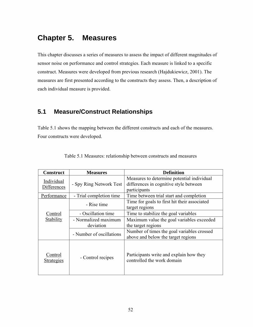
simulation. Calculations are based on industrial average levels of sensor noise............ 44 Table 4.1 Demographic information of participants in all three studies ................................ 47 Table 5.1 Measures: relationship between constructs and measures...................................... 52 Table 5.2 Measures used to assess the impact of sensor noise on performance and control

strategies ......................................................................................................................... 54 Table 5.3 Criteria for relative success in dealing with increased magnitude of sensor noise for

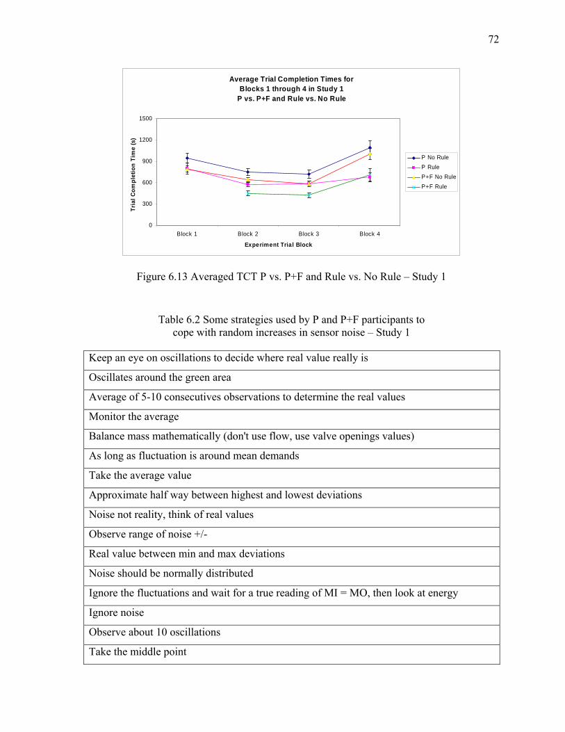
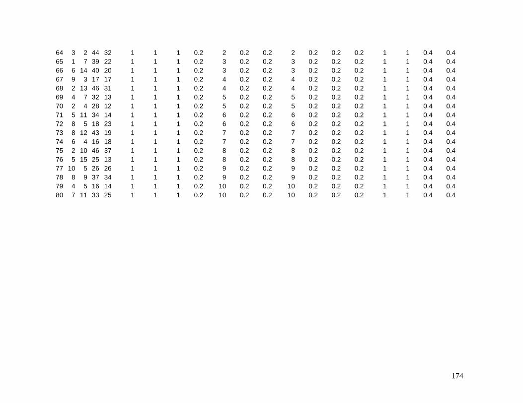
trial completion times ..................................................................................................... 55 Table 6.1 Distribution of scaling multipliers for trials 61 to 80 – Study 1............................. 61 Table 6.2 Some strategies used by P and P+F participants to cope with random increases in

sensor noise – Study 1 .................................................................................................... 72 Table 7.1 Distribution of scaling multipliers for trials 61 to 110 – Study 2........................... 78 Table 7.2 Some strategies used by P and P+F participants to cope with random increases in

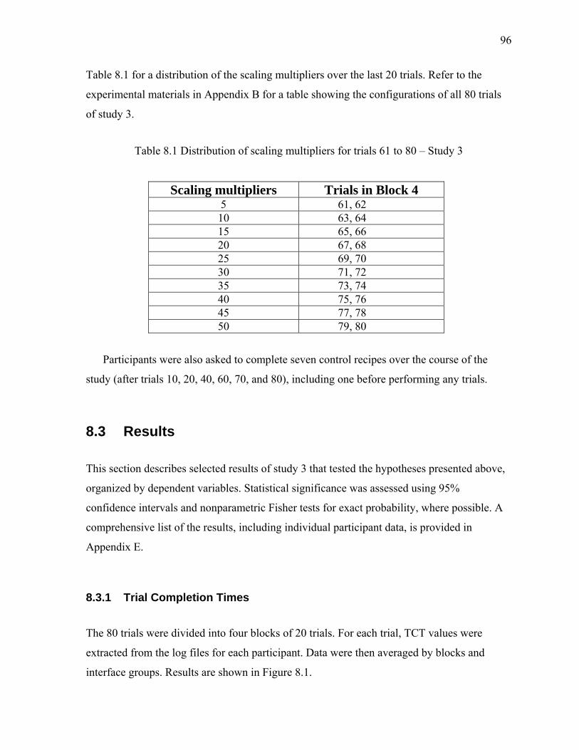
sensor noise – Study 2 .................................................................................................... 88 Table 8.1 Distribution of scaling multipliers for trials 61 to 80 – Study 3............................. 96 Table 8.2 Some strategies used by P+S and P+F participants to cope with random increases

in sensor noise – Study 3 .............................................................................................. 106 Table 9.1 Pearson correlation coefficients between output and temperature demands and

performance and control stability dependent measures for all three studies ................ 118

ix

LIST OF FIGURES

Figure 1.1 Potential effects of sensor noise on interface and the human operator (adapted from Vicente and Rasmussen, 1992). ............................................................................... 3

Figure 1.2 Possible sensor failures and scope of this research ................................................. 5 Figure 2.1 Comparison between human senses and machine sensors of technological systems

(modified from Hauptmann, 1993)................................................................................... 8 Figure 2.2 Human-aided control of a modification tank system (modified from Johnson, 1997)

.......................................................................................................................................... 8 Figure 2.3 Automatic-aided control of a modification tank system (modified from Johnson,

1997) ................................................................................................................................. 9 Figure 2.4 Accuracy of a sensor represented with an accuracy band....................................... 9 Figure 2.5 Emergent feature showing the relationship between Mass Input and Mass Output

in a feedwater process. In this configural display, the Mass Input bar graph is derived from raw sensor data (e.g., flow rates of several input valves) (adapted from Vicente, 1999). .............................................................................................................................. 11

Figure 2.6 Potential instrumentation errors and their effects on displays of measurement signals (Anyakora and Lees, 1974). ............................................................................... 13

Figure 3.1 The DURESS II microworld. The maximum and minimum ranges of each

component are shown in square brackets (adapted from Vicente and Rasmussen, 1990)......................................................................................................................................... 19

Figure 3.2 Work domain analysis of DURESS II (adapted from Bisantz & Vicente, 1994; Hajdukiewicz, 2000)....................................................................................................... 20

Figure 3.3 Full AH of DURESS II including all means-ends links (Modified from Vicente, 1999) ............................................................................................................................... 21

Figure 3.4 Control task parts in a DURESS II start-up task................................................... 22 Figure 3.5 Opportunities to configure DURESS II during start-up........................................ 22 Figure 3.6 Full sensor-annotated AH of the DURESS II simulation ..................................... 28 Figure 3.7 P Interface for DURESS II – displays primarily physical information about the

work domain and goal regions........................................................................................ 29 Figure 3.8 AH state information available (bolded) on the P interface of DURESS II. ........ 31 Figure 3.9 Sensor-annotated AH for the P interface of DURESS II. ..................................... 32 Figure 3.10 P+S Interface for DURESS II – displays primarily physical information about

the work domain as well as all fifteen sensor data available in the DURESS II simulation ....................................................................................................................... 33

Figure 3.11 AH state information available (bolded) on the P+S interface of DURESS II. .. 34 Figure 3.12 Sensor-annotated AH for the P+S interface of DURESS II................................ 35 Figure 3.13 P+F Interface for DURESS II – displays both physical and functional

information about the work domain ............................................................................... 36 Figure 3.14 AH state information available (bolded) on the P+F interface of DURESS II ... 37 Figure 3.15 Sensor-annotated AH for the P+F interface of DURESS II................................ 38 Figure 3.16 Normal distribution of 5000 random numbers representing white normally

distributed Gaussian noise with zero mean and unit of variance.................................... 39

x

Figure 3.17 White noise generation module added to the DURESS II simulation ................ 40 Figure 3.18 Effects of different noise magnitudes on the Mass In – Mass Out emergent

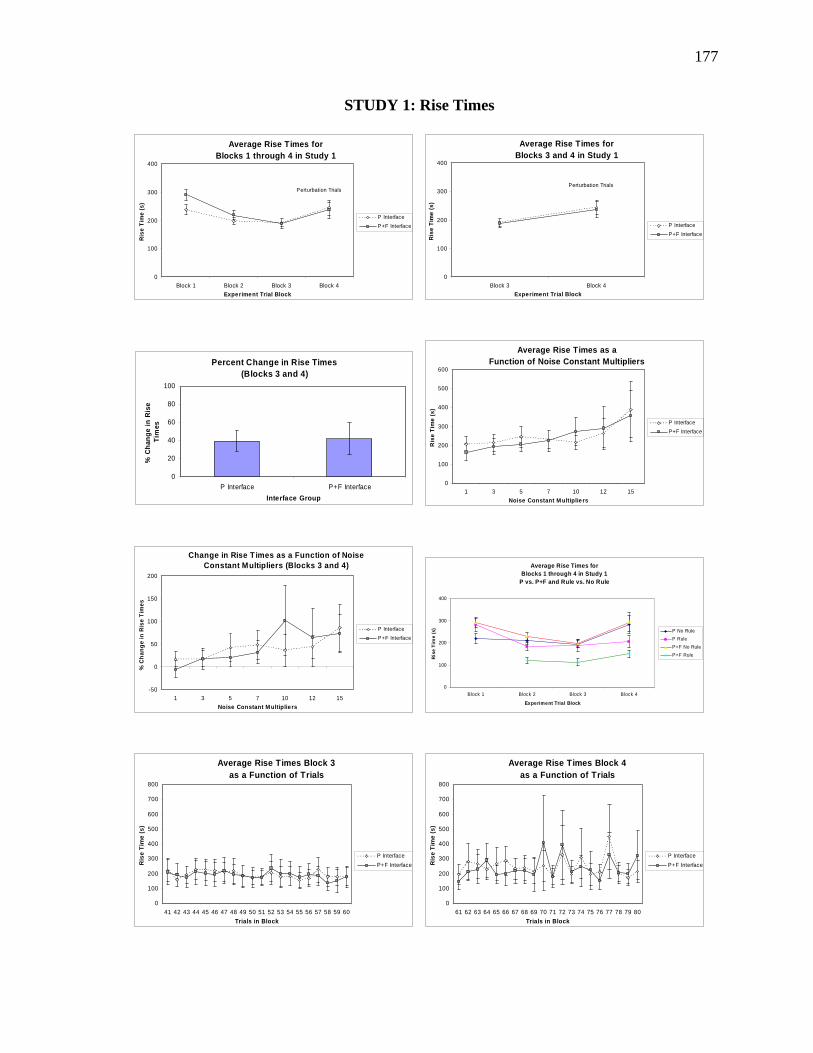
feature of DURESS III.................................................................................................... 43 Figure 4.1 Experimental apparatus – DURESS III................................................................. 48 Figure 5.1 Goal variable measures ......................................................................................... 56 Figure 6.1 Averaged TCT for each of the four experimental blocks – Study 1 ..................... 62 Figure 6.2 Difference in TCT between block 3 and block 4 – Study 1.................................. 63 Figure 6.3 Percentage of change between block 3 and block 4 – Study 1 ............................. 63 Figure 6.4 Averaged TCT as a function of noise constant multipliers in block 4 – Study 1.. 64 Figure 6.5 Averaged Rise Time for each of the four experimental blocks – Study 1 ............ 66 Figure 6.6 Averaged Oscillation Time for each of the four experimental blocks – Study 1.. 66 Figure 6.7 Averaged Number of Oscillations for each of the four experimental blocks –

Study 1 ............................................................................................................................ 66 Figure 6.8 Averaged Maximum Deviation for each of the four experimental blocks – Study 1

........................................................................................................................................ 67 Figure 6.9 Changes in actions dependent on perturbation context for all seven control recipes

of study 1 ........................................................................................................................ 68 Figure 6.10 P+F participants who reported using emergent features – Study 1..................... 69 Figure 6.11 Number of participants who reported using lower-level relationships in study 1

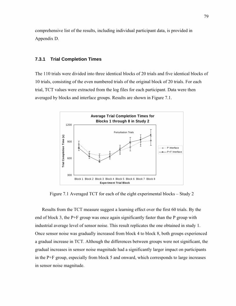
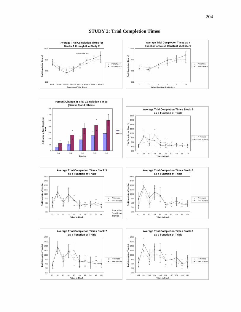
........................................................................................................................................ 70 Figure 6.12 Number of participants who reported using the heater rule in study 1 ............... 71 Figure 6.13 Averaged TCT P vs. P+F and Rule vs. No Rule – Study 1................................. 72 Figure 7.1 Averaged TCT for each of the eight experimental blocks – Study 2.................... 79 Figure 7.2 Percentage of change between block 3 and blocks 4 to 8 – Study 2..................... 80 Figure 7.3 Averaged TCT as a function of noise constant multipliers – Study 2................... 80 Figure 7.4 Averaged Rise Time for each of the eight experimental blocks – Study 2........... 82 Figure 7.5 Averaged Oscillation Time for each of the eight experimental blocks – Study 2 83 Figure 7.6 Averaged Number of Oscillations for each of the eight experimental blocks –

Study 2 ............................................................................................................................ 83 Figure 7.7 Averaged Maximum Deviation for each of the eight experimental blocks – Study

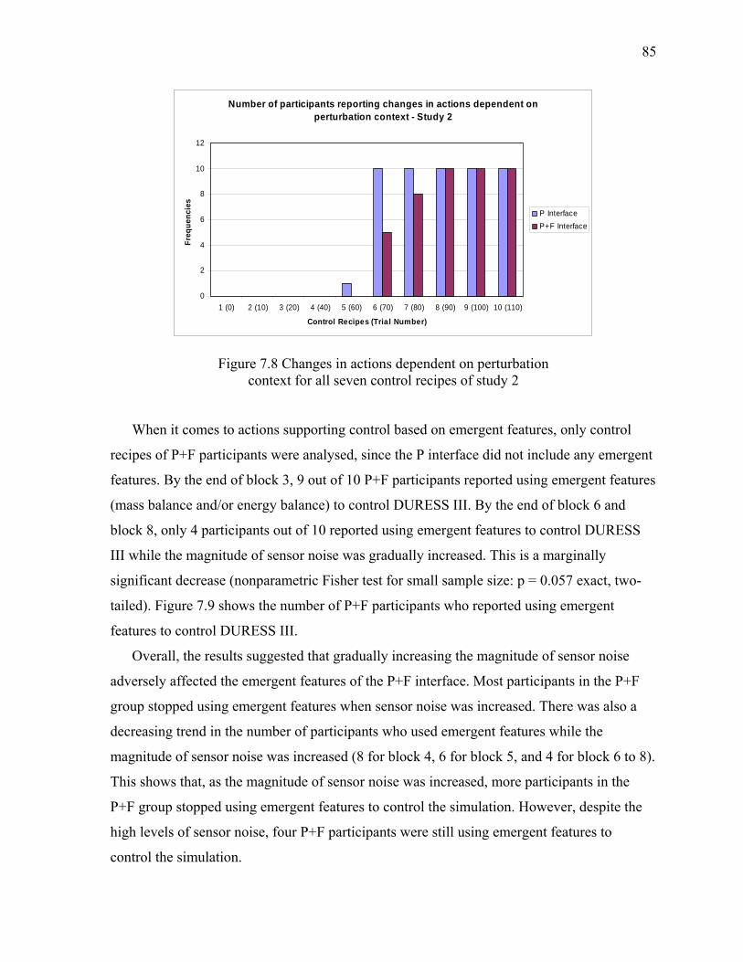
2 ...................................................................................................................................... 83 Figure 7.8 Changes in actions dependent on perturbation context for all seven control recipes

of study 2 ........................................................................................................................ 85 Figure 7.9 P+F participants who reported using emergent features – Study 2....................... 86 Figure 7.10 Number of participants who reported using lower-level relationships in study 2

........................................................................................................................................ 87 Figure 8.1 Averaged TCT for each of the four experimental blocks – Study 3 ..................... 97 Figure 8.2 Difference in TCT between block 3 and block 4 – Study 3.................................. 98 Figure 8.3 Percentage of change between block 3 and block 4 – Study 3 ............................. 98 Figure 8.4 Averaged TCT as a function of noise constant multipliers in block 4 – Study 3.. 99 Figure 8.5 Averaged Rise Time for each of the four experimental blocks – Study 3 .......... 101

xi

Figure 8.6 Averaged Oscillation Time for each of the four experimental blocks – Study 3 101 Figure 8.7 Averaged Number of Oscillations for each of the four experimental blocks –

Study 3 .......................................................................................................................... 101 Figure 8.8 Averaged Maximum Deviation for each of the four experimental blocks – Study 3

...................................................................................................................................... 102 Figure 8.9 Changes in actions dependent on perturbation context for all seven control recipes

of study 3 ...................................................................................................................... 103 Figure 8.10 P+F participants who reported using emergent features – Study 3................... 104 Figure 8.11 Number of participants who reported using lower-level relationships in study 3

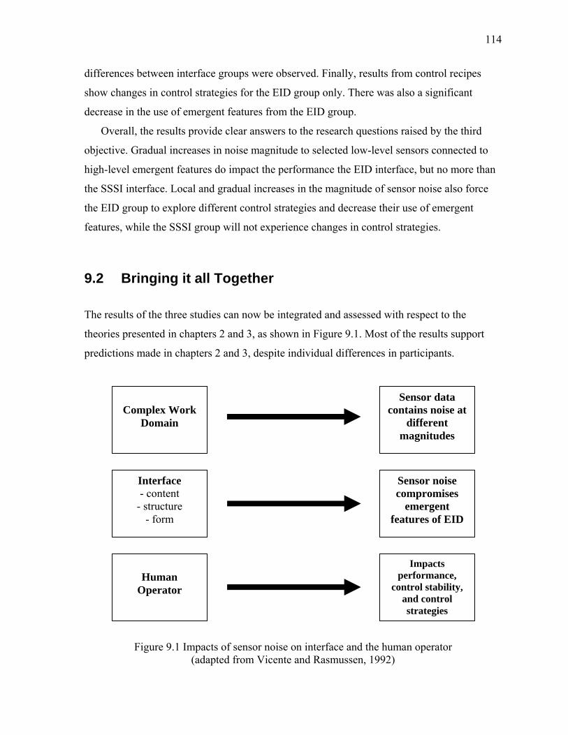
...................................................................................................................................... 105 Figure 9.1 Impacts of sensor noise on interface and the human operator (adapted from

Vicente and Rasmussen, 1992)..................................................................................... 114

xii

LIST OF APPENDICES

Appendix A White Noise C Code ........................................................................................ 136 Appendix B Experimental Materials .................................................................................... 139 Appendix C Detailed Results of Study 1.............................................................................. 175 Appendix D Detailed Results of Study 2.............................................................................. 203 Appendix E Detailed Results of Study 3 .............................................................................. 231

1

Chapter 1. Introduction In an age of rapidly changing technology, modern process control plants, such as nuclear

power plants and petrochemical plants, are becoming more complex than ever. Such plants

must be monitored by human operators, imposing high workload on the workers and

continuously raising safety issues. To cope with such great technological changes, cognitive

engineers have made an effort to develop interface design frameworks that help operators to

cope with highly demanding tasks (e.g., Ecological Interface Design; Vicente and Rasmussen,

1992). For all interface design frameworks, sensors located throughout the plant are of

primary importance, as they provide most of the data to be portrayed on the control displays.

However, sensors are by nature noisy, which can have an effect on both the display

structures and operators’ control strategies. This dissertation aims at understanding the

relationship between sensor noise, interface design, and operators.

1.1 Background

Modern process control plants are made of several components which are often structured in

a complex manner. To monitor the interactions between all the different components, sensors

are installed at strategic locations throughout the plant (Johnson, 1997). One of the main

functions of sensors is to probe the physical plant (world) and send the acquired information

to an interface, so that it can be monitored by operators.

Despite the current state of technology, information transmitted by the instrumentation

and control equipment is often noisy (Stein, 1969; Reising and Sanderson, 2002b). Therefore,

data about the state of world will be uncertain; potentially affecting both the display content

and the ways operators will control the equipment. This dissertation investigates potential

effects of sensor noise on the Ecological Interface Design (EID) framework. This work aims

to contribute to both academic and industrial practices.

EID is a framework for designing human-machine interfaces for complex systems

(Vicente and Rasmussen, 1992). The approach is intended to support design for adaptation to

allow workers to cope with novelty and change. EID uses the Abstract Hierarchy (AH;

2

Rasmussen, 1985) as a modelling tool to represent the work domain in terms of information

content and structure. These requirements may then be transformed to an appropriate

interface form taking into account the capabilities and limitations of the human operator.

Over the past years, the framework has been applied to a variety of domains (e.g., aviation,

medicine, process control; see Vicente, 2002 for a comprehensive review). To implement

EID interfaces, several sensors must be used to acquire data from the work domain and

display them in meaningful graphical representations.

When EID was introduced, Vicente and Rasmussen (1992) pointed out that noisy sensors

are a source of data uncertainty that could compromise the robustness of EID interfaces (cf.

Reising and Sanderson, 2002b). Such interfaces will often include several emergent features

(Pomerantz and Pristach, 1989; Bennett, Toms, and Woods, 1993) that are produced from

relationships between low-level graphical elements1. Because emergent features are derived

from low-level data (which are normally obtained through sensors), sensor noise could

adversely have an effect on high-level constraints to be portrayed on the interface,

compromising the geometric forms of configural displays (Reising and Sanderson, 2002c).

Another important aspect of sensor noise to consider is its effects on operators’ control

strategies. When data about the world is inexact, operators may have to adjust their decision-

making tactics. For instance, when sensor noise is present, operators may have to adapt their

control strategies to account for the uncertain data. Woods (1988) pointed out that collecting

and integrating data which reflect uncertainty (e.g., sensor noise) requires high cognitive

demands. Moreover, he also mentioned that since the data are in part unreliable, different

strategies may have to be explored to control the system efficiently.

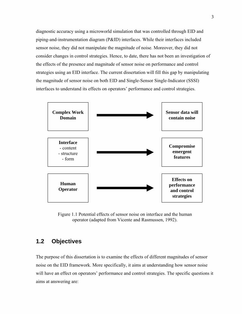
Based on these indications, there seems to be a connection between sensor noise,

configural displays, and control strategies (see Figure 1.1). First, sensor data about the state

of the work domain will contain noise. Second, noise from low-level data may compromise

configural displays and their emergent features. Third, perceived variability due to noise may

have an effect on strategies used by operators. These observations are especially relevant for

interface design frameworks that based on configural displays, such as EID.

To the knowledge of the author, only one study to date is related to the topic of sensors

and EID. Reising and Sanderson (2002c, 2004) studied the impacts of sensor failure on

1 Interfaces that portray higher-order information using emergent features are referred to as configural displays.

3

diagnostic accuracy using a microworld simulation that was controlled through EID and

piping-and-instrumentation diagram (P&ID) interfaces. While their interfaces included

sensor noise, they did not manipulate the magnitude of noise. Moreover, they did not

consider changes in control strategies. Hence, to date, there has not been an investigation of

the effects of the presence and magnitude of sensor noise on performance and control

strategies using an EID interface. The current dissertation will fill this gap by manipulating

the magnitude of sensor noise on both EID and Single-Sensor Single-Indicator (SSSI)

interfaces to understand its effects on operators’ performance and control strategies.

Figure 1.1 Potential effects of sensor noise on interface and the human operator (adapted from Vicente and Rasmussen, 1992).

1.2 Objectives

The purpose of this dissertation is to examine the effects of different magnitudes of sensor

noise on the EID framework. More specifically, it aims at understanding how sensor noise

will have an effect on operators’ performance and control strategies. The specific questions it

aims at answering are:

Complex Work

Domain

Interface - content

- structure - form

Human

Operator

Sensor data will

contain noise

Compromise

emergent features

Effects on performance and control strategies

4

1. What will be the effects of the presence and random magnitude of sensor noise on

operators’ performance and control strategies when using EID versus SSSI

interfaces?

2. Will sensor noise prompt operators to use different control strategies when the

magnitude of the noise is gradually increased globally throughout EID versus

SSSI interfaces? Moreover, how will this manipulation have an effect on

operators’ performance?

3. How will operators’ performance and control strategies be affected when sensor

noise is introduced locally to selected low-level sensors on EID versus SSSI

interfaces? Moreover, how will these local changes have an effect on operators’

performance?

A series of studies to investigate the effects of the presence and magnitude of sensor

noise on operators’ behaviour were conducted on a representative thermal-hydraulic process

simulation. Each study was designed and carried out to answer hypotheses related to the

three objectives listed above.

1.3 Scope of Research

The following assumptions are going to be made throughout this dissertation:

• The term “magnitude of sensor noise” refers to accuracy of a sensor. Accuracy

represents the highest deviation of a value from its true input. In that sense,

accuracy often means inaccuracy and is represented by a plus or minus (+/-) range

in which the sensor is expected to stay.

• The term “perturbation” refers to an increase or decrease in the magnitude of

sensor noise. Other types of sensor failures, such as drift, were not studied.

• The term “industry average sensor noise” refers to a magnitude of sensor noise

similar to the one observed in industrial settings, when sensors are operating

within their normal ranges of accuracy.

• In this dissertation, the bandwidth of noise was not manipulated and was kept

constant at 0.5 Hz.

5

Figure 1.2 illustrates the scope of this research. It shows some possible types of sensor

failures (c.f. Reising, 1999) and points out the scope of this work: to study the effects of

various sensor noise magnitudes globally and locally, complementing previous research

conducted by Reising and Sanderson (2002c, 2004), who studied various types of sensor

failures in the context of sensor versus system failures and instrumentation configurations.

Figure 1.2 Possible sensor failures and scope of this research

1.4 Organization of Dissertation

The remainder of this dissertation is organized into fours parts: Foundations and Measures,

Empirical Studies, General Discussion, and Conclusions. The flow of the dissertation moves

from a theoretical level to an empirical level. The results will then be explained and the

discussions will provide answers to the theoretical issues outlined in the first part. The

chapters organization is as follows:

• Chapter 2 will provide background research on sensor noise and interface design.

It will concentrate on three points of interest: the effects of sensor noise on

configural displays, on operators, and on EID.

• Chapter 3 will present issues related to sensor noise and process control systems.

The DUal Reservoir Simulation System II (DURESS II) system will be

Read zero

Read constant

Erratic noise magnitudes Drift up

Drift down

Displaced reading

Read full

Possible types of sensor failures

Scope of Research • Random magnitude • Increase magnitude • Global perturbations • Local perturbations

6

introduced. A sensor-annotated Abstraction Hierarchy (AH) of DURESS II will

also be presented as well as an analysis of the impact of sensor noise on the

microworld. A description of the updated DURESS III microworld will also be

presented.

• Chapter 4 will describe the experimental protocol used to conduct the three

empirical studies presented in this dissertation.

• Chapter 5 will describe the measures that were used to study the impacts of sensor

noise on operators’ performance and control strategies.

• Chapters 6, 7, and 8 will present the results from three studies using different

types of perturbations to test predictions based on the objectives from chapter 1:

global random perturbations (study 1), global gradually increasing perturbations

(study 2), and local gradually increasing perturbations (study 3).

• Chapter 9 will compare the results from all three studies and draw general

conclusions. Both theoretical and practical implications will be presented.

Empirical results will also be compared to previous results obtained using the

DURESS II microworld.

• Chapter 10 will outline the key findings, relevance, contributions, limitations, and

future research directions.

7

Chapter 2. Foundations

The theory behind this dissertation is based on considerations illustrated in Figure 1.1. First,

knowledge about basic concepts of sensor and sensor noise is needed. Second, a grasp of the

potential effects of sensor noise on graphical displays is required. Finally, an understanding

of the effects of sensor noise on operators’ control strategies is essential. This chapter

discusses these theoretical foundations; in the next chapter, these concepts are transferred to

the domain of process control.

2.1 Instrumentation and Control Equipment

The term sensor is derived from the Latin word sensorium, meaning sensory capability, or

sensus, meaning sense. Given this origin of the word sensor, it seems worthwhile to highlight

the analogy between technical sensors and the senses of human beings. Figure 2.1 illustrates

the comparison between sense organs of humans and machine sensor technology.

Before going further in the discussion of sensors, a definition of the term would be

helpful. The following definition will be used:

A sensor can be defined as a device that receives and responds to a signal or

a stimulus (Fraden, 1997). More specifically, “a sensor converts the physical

dimension which is to be measured into an electrical dimension which can be

processed or transmitted electronically” (Hauptmann, 1993, p. 4).

Figure 2.1 suggests two possible ways of monitoring a control variable: human-aided

control and automation-aided control. Both types of control are illustrated in Figure 2.2 and

Figure 2.3. Figure 2.2 shows a modification tank system to allow regulation of the level by a

human. The human can regulate the level of the tank by using the sight tube (S) to compare

the level (h) to the set point (H). The human can then adjust the valve accordingly to increase

or decrease the level. Figure 2.3 shows the same system regulated by an automatic controller.

The automatic level-control system replaces the human by a controller and uses a sensor to

measure the level.

8

Figure 2.1 Comparison between human senses and machine sensors of technological systems (modified from Hauptmann, 1993)

Figure 2.2 Human-aided control of a modification tank system (modified from Johnson, 1997)

9

Figure 2.3 Automatic-aided control of a modification tank system (modified from Johnson, 1997)

Fraden (1997) outlines several characteristics of modern sensor technology. For example:

resolution, sensitivity, stability, speed of response, operating cost, hysteresis, etc. A very

important characteristic of sensors, especially for the purpose of this dissertation, is accuracy.

Accuracy represents the highest deviation of a value from its true input. In that sense,

accuracy often means inaccuracy and is represented by a plus or minus (+/-) range in which

the sensor is expected to operate. This range is often referred to as sensor noise (Fraden,

1997). Figure 2.4 shows a graphical representation of the concept of sensor accuracy. In this

case, the true value (reading) is surrounded by an accuracy band, representing the plus or

minus (+/-) range in which the sensor is expected to function under normal operating

conditions.

Figure 2.4 Accuracy of a sensor represented with an accuracy band

10

According to Johnson (1997), accuracy can appear in several forms:

1. Measured variable: for example, an accuracy of ± 2ºC would mean that true

temperature reading would be uncertain by ± 2ºC

2. Percentage of the instrument full-scale reading: for example, an accuracy of ± 2%

in a 25ºC scale would mean that true temperature reading would be uncertain by

± 0.5ºC

3. Percentage of instrument span: for example, an accuracy of ± 3% of a span for a

20ºC – 50ºC range of temperature would be uncertain by ± 0.9ºC

4. Percentage of actual reading: for example, an accuracy of ± 2% on a thermometer

reading would be uncertain by ± 0.04ºC if the reading is 2ºC

Several factors can influence the accuracy of sensors and thus, the magnitude of sensor

noise. For example, the calibration of the device will have an effect on its measurement

range. That is, when a device is poorly calibrated, its calibrated span will change, potentially

affecting the accuracy of the device (see number 3 above). Other factors such as

environmental factors can also change the accuracy of a sensor. As shown in Figure 2.1,

sensor data in automatic-aided control systems will be portrayed on a display for humans to

monitor. In that sense, sensor accuracy will be translated into uncertainty, which can affect

display content, structure, and form as well as human operators (see Figure 1.1). The next

two sections will look at these issues into more details.

2.2 Effects of Sensor Noise on Configural Displays

One important aspect of sensor noise to consider is its impact on graphical elements. For

example, configural displays and their emergent features may be adversely affected by

sensor noise. Before going any further, it is worth mentioning that are multiple definitions of

the term emergent features. For the purpose of this work, the term emergent features shall

refer to “a property of the configuration of individual variables that emerges on the display to

signal a significant task-relevant, integrated variable” (Wickens, Lee, Liu, and Gordon-

Becker, 2004, p. 205). One of the key aspects of emergent features is that they map to task-

related variables. In that sense, emergent features will help information integration if they are

mapped into key variables of the task.

11

Pomerantz (1981) has referred to emergent features as properties of an object that can be

produced when configurable dimensions are combined. Such configurations that portray

integrated information using emergent features are referred to as configural displays. “A

configural display represents high-level constraints of the domain through the relationships

among the low-level data that define the constraint” (Bennett, Toms, and Woods, 1993, p.

72). Computer interfaces that capitalize upon graphical representation of a process through

the use of emergent features have several advantages. For example, emergent features will

often represent the constraints on the system in ways that these constraints can be easily

perceived. In fact, the direct perception of these emergent features can replace the more

cognitively demanding computation of derived quantities (Bennett and Flach, 1992). Also,

emergent features will perceptually signal a departure from normality and in some cases may

also help diagnose the nature of a failure.

Figure 2.5 shows an example of an emergent feature. That is, the property of the

configuration of individual variables (in this case mass input and mass output) emerges on

the display to signal a significant, task-relevant, integrated variable (slope of the line). Since

emergent features are derived from low-level data (which are normally obtained through

physical sensors), sensor noise could adversely affect high-level constraints to be portrayed

on the interface, compromising the geometric forms of configural displays (Reising and

Sanderson, 2002b, 2002c).

Figure 2.5 Emergent feature showing the relationship between Mass Input and Mass Output in a feedwater process. In this configural display, the Mass Input bar graph is derived from

raw sensor data (e.g., flow rates of several input valves) (adapted from Vicente, 1999).

A similar argument was made by Vicente, Moray, Lee, Rasmussen, Jones, Brock, and

Djemil (1996) who pointed out that sensor failures could create distortions in emergent

12

features, detrimentally affecting the behaviour of operators. Conversely, they also suggested

that any distortions due to sensor failures may also create salient information to help

operators in detecting problems.

Vicente (2002) also mentioned two possible effects of sensor noise on EID interfaces.

First, the robustness of EID interfaces might not be compromised by sensor noise due to the

redundant constraints portrayed on the interface. Second, as mentioned in Vicente et al.

(1996), sensor noise may also confuse operators in their ability to distinguish between the

displayed state and the true state of the work domain. Hence, while sensor noise can

potentially disturb configural displays and their emergent features, it may also help operators

in detecting malfunctions.

This dual impact of sensor noise on emergent features is supported by research in the

field of uncertainty and graphical displays. For example, Pang, Wittenbrink, and Lodha

(1997) argued that displaying information in a holistic fashion (e.g., emergent features)

provides users with a better understanding of the data. Moreover, they also suggest using

such displays to help users coping with uncertainty that may be introduced in the data.

Another study conducted by Wittenbrink, Saxon, Furman, Pang, and Lodha (1996) suggests

that deviations from normal states are easily recognized when data from multiples sensors

are integrated into holistic graphical representations. Finally, Finger and Bisantz (2002)

suggest that the use of distorted or degraded images is a viable way to convey situational

uncertainty. All these studies demonstrate that while sensor noise can adversely have an

effect on configural displays and their emergent features, it can also be beneficial in coping

with situational uncertainty. However, none of these studies specifically investigated the

impact of sensor noise on performance.

Ways in which operators will detect malfunctions and uncertainties depend on the type of

error, the type of display used to convey information, and the operator’s sensitivity to

changes in dynamic graphical objects (Jessa and Burns, 2005). Anyakora and Lees (1974)

describe some typical instrumentation errors and their effects on graphical displays. Figure

2.6 shows displays of measurement signals with respect to potential types of errors

(Anyakora and Lees, 1974).

13

Figure 2.6 Potential instrumentation errors and their effects on displays of measurement signals (Anyakora and Lees, 1974).

As pointed out in Chapter 1 (Figure 1.2), this dissertation focuses on the issue of sensor

noise, represented as Reading erratic in Figure 2.6. One can see how erratic readings disturb

the measurement signal and may send an indication that a malfunction is present or

potentially confuse operators. Of course, erratic readings may also go undetected if the

magnitude of the noise is low (see section 3.4.1 for more details).

2.3 Effects of Sensor Noise on Operators

Sensor noise can also have an effect on operator’s performance and control strategies. One of

the important tasks for operators of complex systems is to collect and integrate data to

understand the current state of the plant. When data about the world is inexact, operators may

14

have to adjust their decision-making tactics (Endsley, 2003). For instance, when sensor noise

is present, operators may have to adapt their control strategy to account for the uncertain data.

Woods (1988) pointed out that collecting and integrating data which reflect uncertainty (e.g.,

sensor noise) will require high cognitive demands. Moreover, he also mentioned that since

the data is in part unreliable, different strategies might have to be explored to control the

system efficiently. Finger and Bisantz (2002) also suggest that data uncertainty can have an

effect on decisions and actions made by operators since the data have the potential of losing

their real meanings and more interpretation might be required.

Endsley (2003) presented a number of control strategies used by operators of complex

systems to manage uncertainty, some of which related to dealing with noisy data. For

example, she pointed out that when faced with uncertain data, operators of complex systems

will often (1) search for more information, (2) rely on typical default values, (3) try to

determine which data source is incorrect or the reliability of different sources, (4) try to

reduce uncertainty to an acceptable level to continue operation, (5) go into contingency

planning, and (6) channel their attention to only specific pieces of information. All these are

potential strategies operators might use to cope with uncertainty in graphical displays.

Endsley (2003) argued that good display design is not only about displaying information, but

also about supporting these active strategies for dealing with the uncertainties involved in the

collection of information.

Endsley (2003) also proposed design guidelines to support operator’s ability to determine

how much confidence to place in information that is presented on graphical displays. For

example: (1) explicitly have ways to identify missing information (e.g., missing sensor data),

(2) support sensor reliability assessments by providing data on sensor reliability, (3) use data

salience to support certainty, (4) represent information timeliness, (5) support uncertainty

management, and (6) support assessments of confidence in composite data.

This last point is related to the research conducted in this dissertation. That is, when the

output of many lower-level sensors are merged into one higher-level graphical element, it

can be difficult for operators to assess how much confidence to place in the composite data,

especially when the reliability of the underlying data becomes hidden or lost due to sensor

failures (e.g., sensor noise). In this case, it is necessary to provide operators with clear ways

of identifying sources of the composite data to help them assess the degree of confidence

15

they should have in the merged data. Altogether, these studies and recommendations

emphasize the importance of investigating the effects of uncertainty on control strategies.

2.4 Effects of Sensor Noise on Ecological Interface Design

EID (Vicente and Rasmussen, 1992) is a framework for designing human-machine interfaces

for complex systems. Over the past years, the framework has been applied to a variety of

domains such as process control, medical systems, and training and education (see Vicente,

2002, for a comprehensive review). To implement EID interfaces, several sensors are used to

acquire data about the work domain and display them in meaningful graphical

representations, creating emergent features, like the one shown in Figure 2.5.

When EID was introduced, Vicente and Rasmussen (1992) pointed out that noisy sensors

are a source of data uncertainty that could compromise the robustness of EID interfaces.

More recently, Vicente (2002) mentioned that research on how sensor noise and sensor

failure affect workers’ performance using an EID interface is still needed today. Indeed,

while a large number of studies have shown that EID improves performance, only one study

(Reising and Sanderson, 2002c, 2004) to date is related to the topic of sensors and EID.

Reising and Sanderson (2002c, 2004) studied the impacts of sensor and system failures

on diagnostic accuracy using the Pasteurizer II microworld (Reising and Sanderson, 2002a).

They were especially interested in the issue of topographic versus derivational failures.

Topographic failures occur when a physical reading from a sensor is incorrect, while

derivational failures occur when higher-order information, derived from inaccurate physical

readings, is incorrect.

Interfaces for the Pasteurizer II simulation were designed according to two independent

variables: Interface Design Framework (EID vs. P&ID – piping-and-instrumentation diagram

interface) and Instrumentation (Minimal vs. Maximal), resulting in four groups: EID.Max,

EID.Min, P&ID.Max, and P&ID.Min. The EID.Max interface was derivationally adequate,

while the EID.Min was derivationally inadequate. On the other hand, the P&ID.Max

interface was topographically adequate, while the P&ID.Min was typographically inadequate.

Failures were of two types: system failures (e.g., leak) and sensor failures (e.g., drift down).

Their research examined the extent to which minimal versus maximal instrumentation

16

configurations affected overall failure diagnosis, sensor failure diagnosis, and variability in

control performance. All sensors, when behaving under normal operating conditions,

exhibited representative sensor noise (Reising, 1999). Only sensor failure diagnosis results

will be described here.

Results suggest that the EID.Max condition supported better sensor failure diagnosis than

both P&ID interfaces (Max and Min). However, the advantage of the EID framework was

lost in the EID.Min condition, reducing the percentage of correct sensor failure diagnoses

(Reising and Sanderson, 2004). These results suggest that the EID framework will support

better sensor failure diagnoses only when the interface contains enough sensors to ensure that

derivational information is adequate and is available to help operators in their problem-

solving strategies. No significant control performance differences between the P&ID and

EID interfaces were observed (Reising and Sanderson, 2000). However, it is important to

note that their experiment was not set up to specifically study control performance.

While the interfaces in Reising and Sanderson’s study included sensor noise, they did

not manipulate the magnitude of that noise. Moreover, they did not consider changes in

control strategies. Hence, to date, there has not been an investigation of the effects of

different magnitudes of sensor noise on performance and control strategies using an EID

interface.

This dissertation will fill this gap by manipulating the magnitude of sensor noise on both

EID and SSSI interfaces to understand its effects on operators’ performance and control

strategies. This is an important topic to investigate. Indeed, Anyakora and Lees (1974)

pointed out that detection of malfunction in measuring instruments is a task every operator in

industrial settings must perform. Moreover, Reising and Sanderson (2002b) also pointed out

that problems with sensors could adversely have an effect on the graphical representations

portrayed on EID interfaces. In that sense, determining the robustness of EID interfaces

under noisy sensors will have a major impact on the applicability of the framework in real

industrial settings (Watanabe, 2001).

17

2.5 Summary

The theory and background presented in this chapter illustrate the relationships between

sensor noise, configural displays, and control strategies, as shown in Figure 1.1. Information

on sensor technology demonstrates how accuracy of sensors will ultimately result in sensor

noise. This noise can be of different magnitudes, depending on several factors, such as sensor

calibration and environmental conditions. Unless filtered, sensor noise will eventually make

its way to the computer display (Figure 2.1), introducing uncertainty in the data. Moreover,

when several physical sensors are merged into one single graphical element, the noise will be

propagated into the calculations, affecting the output of the derivation process. In that sense,

configural displays and their emergent features will be adversely affected by sensor noise.

Ultimately, sensor noise and distorted emergent features will have an effect on the ways in

which operators control the system. Added uncertainty is likely to prompt operators to look

at different control strategies and decision-making tactics.

In this dissertation, the impacts of sensor noise on operators’ performance and control

strategies will be assessed using the EID framework, since EID interfaces are based on

configural displays containing emergent features. The next chapter applies the concepts

outlined in this chapter to the domain of process control using DURESS II, a microworld

simulator.

18

Chapter 3. Sensor Noise in Process Control

This chapter describes the impacts of sensor noise in process control. To illustrate how

sensor noise has an effect on interface structure of process control systems, the details of the

DURESS II simulation are discussed; this platform was used as the testbed for this research.

It is important to first understand the structure of the simulation as well as its operating

characteristics. Then, a detailed description of the control task and control strategies is

presented. Using a sensor-annotated Abstract Hierarchy (AH; Rasmussen, 1985), it is

possible to derive the impacts of sensor noise on the emergent features of DURESS II.

Finally, a description and example of the new updated DURESS III is provided.

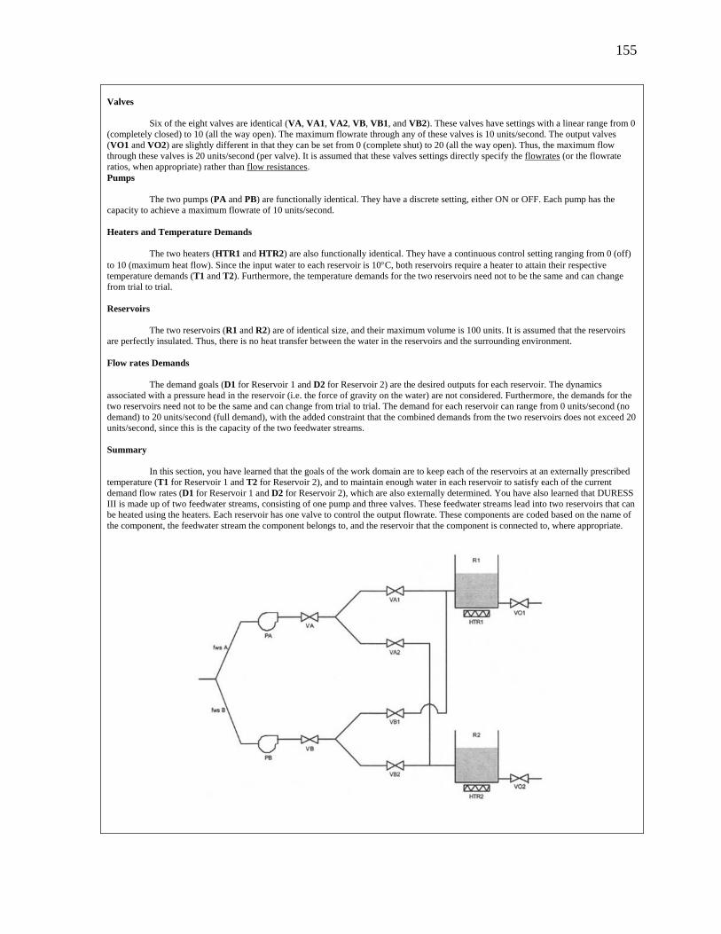
3.1 Description of DURESS II

DURESS II (DUal REservoir Simulation System; Vicente, 1991; Pawlak and Vicente, 1996)

is a representative thermal-hydraulic process microworld (see Figure 3.1) that was used in

this research. It consists of two redundant feedwater streams, fws A and fws B. These

streams can be configured to supply water to two reservoirs: Reservoir 1 and Reservoir 2.

The goals of the work domain are to keep each of the reservoirs at an externally determined

temperature (T1g for Reservoir 1 and T2g for Reservoir 2), and to maintain enough water in

each reservoir to satisfy each of the current demand flow rates (D1g for Reservoir 1 and D2g

for Reservoir 2), which are also externally determined. To satisfy these goals, operators have

control over six input valves (VA, VB, VA1, VA2, VB1, and VB2), two output valves (VO1

and VO2), two pumps (PA and PB), and two heaters (HTR1 and HTR2) within the numerical

ranges specified for each component (see Figure 3.1).

3.1.1 Work Domain representation

Figure 3.2 provides an outline of the work domain representation that was developed for

DURESS II (Vicente & Rasmussen, 1990; Bisantz & Vicente, 1994). Constraints and

19

Figure 3.1 The DURESS II microworld. The maximum and minimum ranges of each component are shown in square brackets (adapted from Vicente and Rasmussen, 1990).

relations underlying DURESS II were modelled using the AH framework. There are three

levels of resolution in the AH space connected by part-whole links (System, Subsystem, and

Component). There are also five levels of abstraction connected by structural means-ends

links (Physical Form, Physical Function, Generalized Function, Abstract Function, and

Functional Purpose). The first step towards understanding a system using the AH is to

identify the components, constraints, relations, and equations that dictate the behaviour of the

system. Vicente (1999) presents a series of equations, as well as their purposes, which

explain the functioning of DURESS II (see, Vicente, 1999, Table 6.3, p. 146). Those

equations are used to understand the essential principles that govern DURESS II.

At the higher levels of abstraction (i.e., Functional Purpose), one can find the purpose of

the system, while at the lower levels (i.e., Physical Function), one will find system

components and their physical properties. The middle levels (i.e., Abstract Function and

Generalized Function) show the connections between the purpose and the physical

components of the system. Hence, the AH shows how certain configurations of components

will achieve the purpose of the system, and what functions are needed for the purpose to be

accomplished, given the system’s components and their properties. Note that the bottom

level of Physical Form is not used here since it refers to the physical location and appearance

of the work domain, features that are not particularly meaningful in a microworld simulation

20

like DURESS II. The full AH of DURESS II is shown in Figure 3.3. Refer to the

experimental materials in Appendix B for a list of the acronyms.

Aggregation - Decomposition

FunctionalPurpose

AbstractFunction

GeneralizedFunction

PhysicalFunction

PhysicalForm

Whole System(DURESS)

Subsystems(Reservoir) Components

Appearance& Location

ComponentStates

Mass/EnergyTopology

Liquid Flow &Heat Transfer

Outputs toEnvironment

Physical -Functional

PA VA VA1 VA2 PB VB VB1 VB2 HTR1 HTR2 R1 R2 VO1 VO2

FPA FVA FVA1 FVA2 FPB FVB FVB1 FVB2 FHTR1 FHTR2 V1 V2 FVO1 FVO2

MI1 M1 MO1 MI2 M 2 MO2 EI2 E2 EO2EI1 E1 EO1

D1 D2 T1 T2

Functional Structure of DURESS II

Figure 3.2 Work domain analysis of DURESS II (adapted from Bisantz & Vicente, 1994; Hajdukiewicz, 2000).

3.1.2 Control Task

A control task is defined as the constrained set of actions that is required to achieve a

particular goal (Vicente, 1999). In this dissertation, participants were required to directly

control DURESS II and to perform a start-up task. The different parts of DURESS II start-up

are discussed discuss below.

In the start-up task of DURESS II, operators are required to bring the simulation from a

shutdown state (i.e., all valves closed, heaters and pumps off, and reservoirs empty) to a

steady-state condition in which all goal variables (D1, T1, D2, T2) are in the target regions

(D1g, T1g, D2g, T2g) simultaneously for five consecutive minutes. There are three parts to

this task (Figure 3.4): rise to target region, oscillation in target region, and steady state in

target region (Yu, Lau, Khayat, Vicente, & Carter, 1997).

In the first part (rise to target), participants configure DURESS II to fill the reservoirs,

heat the water, and get the goal variables in the target regions. Once the goal variables reach

21

Figure 3.3 Full AH of DURESS II including all means-ends links (Modified from Vicente, 1999)

22

the target regions, the second part (oscillation in target) begins. This part requires

participants to make sure all goal variables stay in their target regions. The third part (steady

state in target) requires the participants to maintain the goal variables in the target regions

simultaneously for five consecutive minutes.

TrialStart

TrialEnd

Rise toTarget

Oscillation inTarget

Steady Statein Target

Time (s)

State of Goal Variables

All crossedtarget regions

In target regionssimultaneouslyShutdown

In target regionssimultaneously

for 5 consecutiveminutes

Figure 3.4 Control task parts in a DURESS II start-up task

There are numerous ways of acting on components to accomplish a start-up task. All of

them are constrained by the relevant structural links and functions of the AH. Figure 3.5

shows all the structural opportunities available to accomplish these tasks for both reservoirs;

this is a subset of the entire AH for DURESS II, shown in Figure 3.3.

dM1/dt = MI1 - MO1 dM2/dt = MI2 - MO2

FVA1 FVA2 FVB1 FVB2 FVO1 FVO2

PA VA VA1 VA2 PB VB VB1 VB2 VO1 VO2

Figure 3.5 Opportunities to configure DURESS II during start-up

23

3.1.3 Control Strategies

A control strategy is defined as a category of action sequences that can be used to perform

the control task (Rasmussen, Pejtersen, & Goodstein, 1994). As participants control

DURESS II to meet the target conditions, numerous control strategies can be employed to

perform the various parts of the start-up control task.

Vicente (1999) described three possible strategies to successfully perform a start-up task

on DURESS II. To simplify the discussion, only strategies related to the mass flow are

presented, excluding the energy flow portion of the start-up task. In that sense, heaters

manipulations are not relevant to complete the mass balance portion of the task. The

following is a summary of the start-up task for mass balance as described by Vicente (1999)

and Hajdukiewicz and Vicente (2004a):

1. If combined water demands exceed 20 units/s of flow (capacity of the feedwater

streams), task cannot be performed

2. Assuming the process is totally shut-down, valves VA, VA1, VA2, VB, VB1, and

VB2 must be opened followed by pumps PA and PB.

3. Water must then accumulate in the reservoirs

4. Output demands goals (D1g and D2g) must be checked and VO1 and VO2 must

be set to their respective values

5. Input valves must be fine-tuned to ensure that MASSINPUT = MASSOUPUT

6. Reservoir level must be checked to ensure mass equilibrium

As Vicente (1999) and Hajdukiewicz and Vicente (2004a) pointed out, there are three

possible categories of strategies to successfully complete steps #2 and #5. They are based on

the following equations:

D1 + D2 ≤ 10 units/s (1)

D1 + D2 > 10 units/s; D1 ≤ 10 units/s; D2 ≤ 10 units/s (2)

D1 or D2 > 10 units/s; D1 + D2 ≤ 20 units/s (3)

24

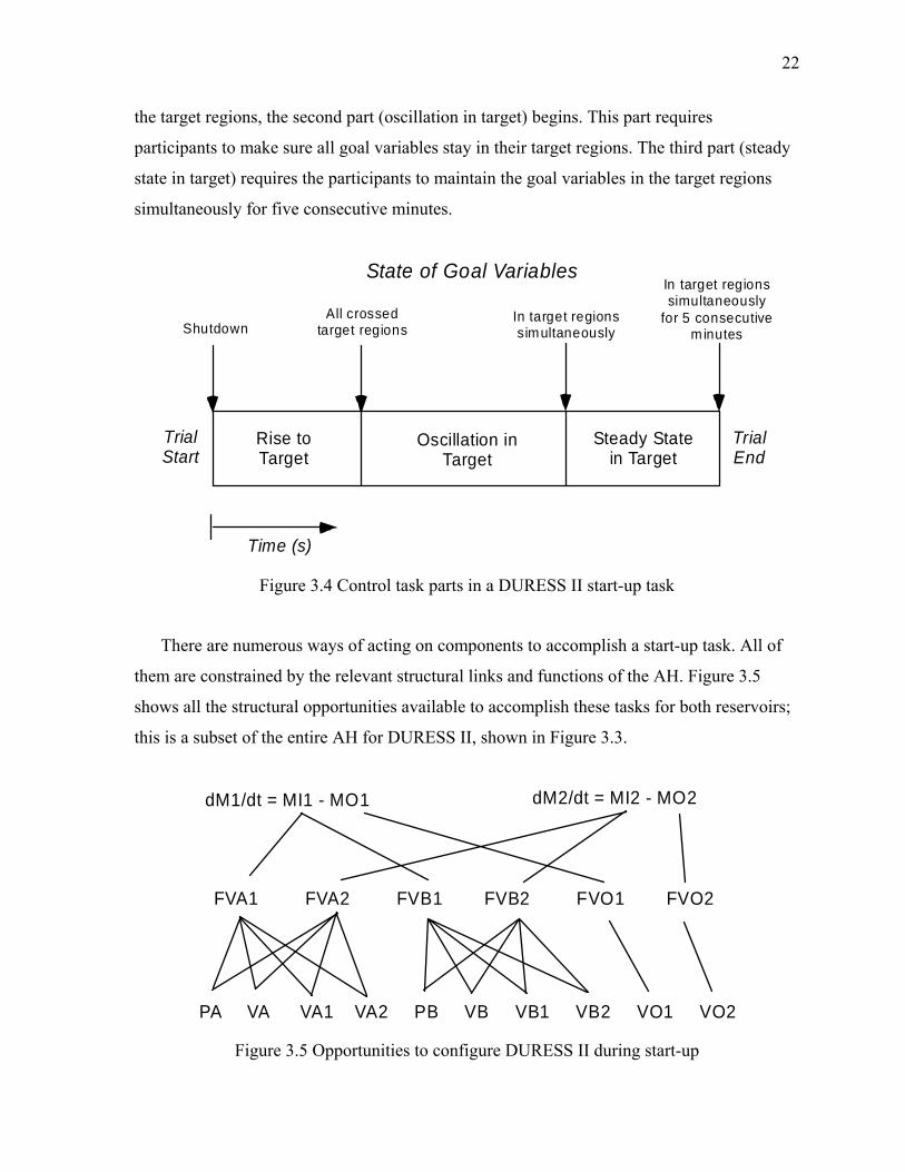
Based on these three equations, Vicente (1999) and Hajdukiewicz and Vicente (2004a)

proposed three different feedwater configuration strategies to complete the mass balance

start-up task. Table 3.1 identifies each category of strategies, followed by a description and

an example.

Table 3.1 Possible feedwater configurations and strategies using the DURESS II simulation. Adapted from Hajdukiewicz and Vicente (2004a).

Feedwater

Configuration Strategy

Description Example

Single

Components: One pump and its connected input valves feed both reservoirs Feasible: D1 + D2 ≤ 10 units/s

Decoupled

Components: Each pump and its connected input valves feed different reservoirs Feasible: D1 ≤ 10 units/s D2 ≤ 10 units/s Necessary: D1 + D2 > 10 units/s

Full

Components: Both pumps and their connected valves feed the reservoirs. At least one pump feeds both reservoirs. Feasible: D1 + D2 ≤ 20 units/s Necessary: D1 or D2 > 10 units/s

25

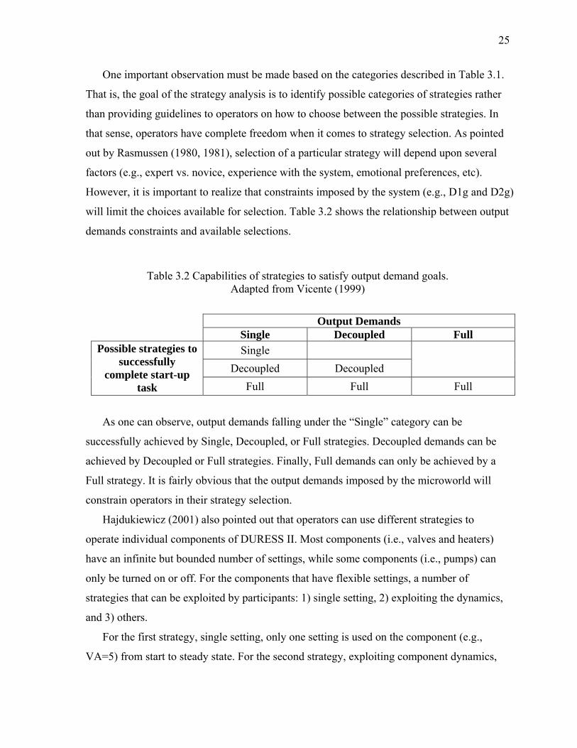
One important observation must be made based on the categories described in Table 3.1.

That is, the goal of the strategy analysis is to identify possible categories of strategies rather

than providing guidelines to operators on how to choose between the possible strategies. In

that sense, operators have complete freedom when it comes to strategy selection. As pointed

out by Rasmussen (1980, 1981), selection of a particular strategy will depend upon several

factors (e.g., expert vs. novice, experience with the system, emotional preferences, etc).

However, it is important to realize that constraints imposed by the system (e.g., D1g and D2g)

will limit the choices available for selection. Table 3.2 shows the relationship between output

demands constraints and available selections.

Table 3.2 Capabilities of strategies to satisfy output demand goals. Adapted from Vicente (1999)

Output Demands

Single Decoupled Full Single

Decoupled Decoupled

Possible strategies to successfully

complete start-up task Full Full Full

As one can observe, output demands falling under the “Single” category can be

successfully achieved by Single, Decoupled, or Full strategies. Decoupled demands can be

achieved by Decoupled or Full strategies. Finally, Full demands can only be achieved by a

Full strategy. It is fairly obvious that the output demands imposed by the microworld will

constrain operators in their strategy selection.

Hajdukiewicz (2001) also pointed out that operators can use different strategies to

operate individual components of DURESS II. Most components (i.e., valves and heaters)

have an infinite but bounded number of settings, while some components (i.e., pumps) can

only be turned on or off. For the components that have flexible settings, a number of

strategies that can be exploited by participants: 1) single setting, 2) exploiting the dynamics,

and 3) others.

For the first strategy, single setting, only one setting is used on the component (e.g.,

VA=5) from start to steady state. For the second strategy, exploiting component dynamics,

26

the valve setting is first put at the end set point until the flow matches the desired value. Then,

the valve setting is reduced so that the flow is stabilized at the desired steady state value.

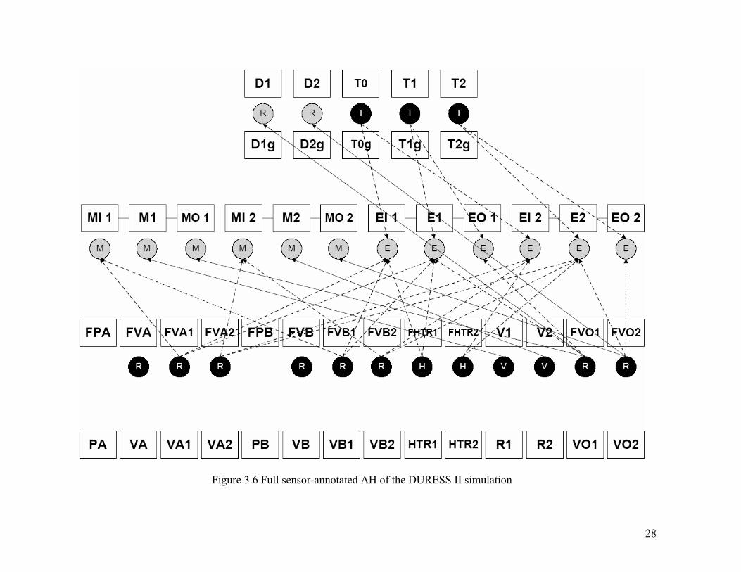
3.2 Sensor-Annotated Abstraction Hierarchy

To analyse the effects of the different instrumentations (sensors) on the ability to provide

information at all the levels of the AH, a sensor-annotated AH (Reising, 1999, Reising and

Sanderson, 2002c) was created. The features of a sensor-annotated AH are explained below:

• Means-ends links between AH levels are removed for clarity and replaced by lines

connecting certain sensors at adjoining levels.

• Below some AH nodes are small circles representing sensors in the DURESS II

system. Sensor nodes include: temperature (T), volume (V), flow rate (R), heat

transfer (H), mass flow rate (M), and energy flow rate (E). Each sensor resides at the

physical form level of the AH, but its significance is represented at higher levels of

the AH (e.g., generalized function).

• Black circles are sensor nodes that are directly sensed as opposed to being derived

mathematically from lower-level sensor data. That is, there exists a physical sensor

for every sensor node represented by a black circle.

• Gray circles indicate variables of DURESS II that have been derived mathematically

from lower-level sensor data rather than sensed directly. Equations for the derivations

can be found in Vicente (1999).

• Black solid lines indicate redundant sensor data portrayed in more than one node of

the AH. For example, data from the flow output valves sensors are also used to

portray mass output flow rates and the output demand goals flow rates. Likewise,

data from the volumes sensors are also used to portray mass inventories of each

reservoir.

• Black dashed lines indicate all the sensors that contribute to a particular mathematical

derivation (gray circles) from lower-level sensor data. For example, the mass input

one flow rate (MI 1) is mathematically derived from the flow rates FVA1 and FVB1.

27

The full sensor-annotated AH for DURESS II is shown in Figure 3.6. Table 3.3 summarizes

the sensor data available in the DURESS II simulation.

Table 3.3 Physical sensors available in the DURESS II simulation as well as mathematically derived variables from lower-level sensor data.

Physical Sensors Mathematically derived variables

Flow rate Valve A (FVA) Variables Contributing sensors Flow rate Valve A1 (FVA1) Output Demand Goal 1 Directly from FVO1

Flow rate Valve A2 (FVA2) Output Demand Goal 2 Directly from FVO2

Flow rate Valve B (FVB) Mass Input 1 FVA1 and FVB1

Flow rate Valve B1 (FVB1) Mass Inventory I Directly from V1

Flow rate Valve B2 (FVB2) Mass Output 1 Directly from FVO1

Volume Reservoir 1 (V1) Mass Input 2 FVA2 and FVB2

Volume Reservoir 2 (V2) Mass Inventory 2 Directly from V2

Heat transfer Heater 1 (FHTR1) Mass Output 2 Directly from FVO2

Heat transfer Heater 2 (FHTR2) Energy Input 1 FVA1, FVB1, FHTR1, T0

Flow rate Output Valve 1 (FVO1) Energy Inventory I FVA1, FVB1, FHTR1, T1, FVO1

Flow rate Output Valve 2 (FVO2) Energy Output 1 T1, FVO1

Temperature Thermometer 0 (T0) Energy Input 2 FVA2, FVB2, FHTR2, T0

Temperature Thermometer 1 (T1) Energy Inventory 2 FVA2, FVB2, FHTR2, T2, FVO2

Temperature Thermometer 2 (T2) Energy Output 2 T2, FVO2

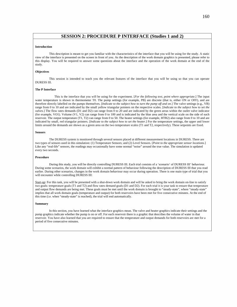
3.2.1 Sensors for P Interface

Two different interfaces (P and P+F) were originally developed for the DURESS II system

(Vicente & Rasmussen, 1990; Pawlak & Vicente, 1996). The P interface (motivated by

mimic design principles) displays primarily physical information about the work domain

with a minimum number of sensors. In contrast, the P+F interface (designed under EID

principles) displays both physical and functional information about the work domain by

28

Figure 3.6 Full sensor-annotated AH of the DURESS II simulation

29

means of configural displays with a maximum number of sensors. Thus, it contains high-

level emergent features based on low-level sensor data. A third interface was created for the

purpose of this research. The P+S interface, like the P interface, displays primarily physical

information about the work domain but with a maximum number of sensors. It does not

contain high-level emergent features, and thus, does not require state variables to be

mathematically derived from lower-level sensor data. This section will describe the P

interface.

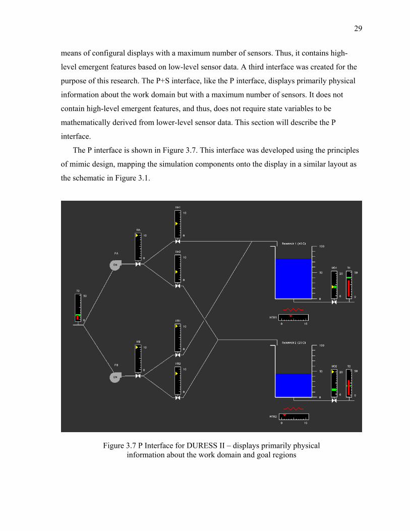
The P interface is shown in Figure 3.7. This interface was developed using the principles

of mimic design, mapping the simulation components onto the display in a similar layout as

the schematic in Figure 3.1.

Figure 3.7 P Interface for DURESS II – displays primarily physical information about the work domain and goal regions

30

Figure 3.8 shows the state information available on the P interface with reference to the

AH of DURESS II (Figure 3.3). Information from primarily the Physical Function and

Functional Purpose levels are displayed on the P interface. In addition, the rate of change of

certain variables (T1, T2, M1, M2, V1, V2) may be deduced over time.

Figure 3.9 shows the sensor-annotated AH for the P interface of DURESS II. Five

physical sensors are portrayed on the P interface (T0, T1, T2, V1, and V2). Two redundant

state variables (M1 and M2) are directly portrayed from sensors V1 and V2.

3.2.2 Sensors for P+S Interface

The P+S interface is shown in Figure 3.10. This interface contains all sensor information

available in the DURESS II simulation. However, it does not contain any emergent feature

and thus, physical sensors do not contribute to any mathematical derivations.

Figure 3.11 shows the state information available on the P+S interface with reference to

the AH of DURESS II (Figure 3.3). Information from the top generalized function level is

displayed in the P+S interface. Information from the abstract function level is generally not

displayed.

Figure 3.12 shows the sensor-annotated AH for the P+S interface of DURESS II. All

fifteen physical sensors are portrayed on the P+S interface (T0, T1, T2, FVA, FVA1, FVA2,

FVB, FVB1, FVB2, FHTR1, FHTR2, V1, V2, FVO1, and FVO2). Six redundant state

variables (D1, D2, M1, MO 1, M2 and MO 2) are directly portrayed from sensors FVO1,

FVO2, V1 and V2.

3.2.3 Sensors for P+F Interface

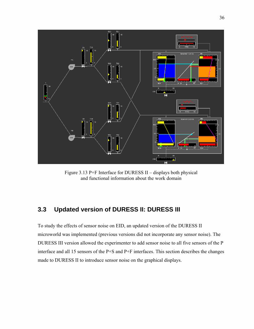
The P+F interface is shown in Figure 3.13. This interface was developed using the principles

of EID, mapping the variables from an AH analysis onto the display.

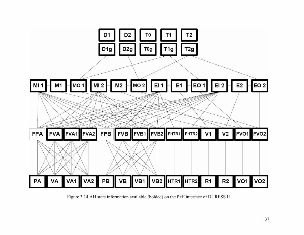
Figure 3.14 shows the state information available on the P+F interface with reference to

the AH of DURESS II (Figure 3.3). Information from the top four levels of the AH are

displayed in the P+F interface. The expected rates of change of some variables (M1, M2, E1,

31

Figure 3.8 AH state information available (bolded) on the P interface of DURESS II.

32

Figure 3.9 Sensor-annotated AH for the P interface of DURESS II.

33

Figure 3.10 P+S Interface for DURESS II – displays primarily physical information about the work domain as well as all fifteen sensor data available in the DURESS II simulation

E2, V1, V2) are shown directly as instantaneous sloped lines (emergent features) on the right

side of Figure 3.13. Finally, integrated graphics showing the relationship between mass,

energy, and temperature is shown in between the mass and energy graphics. These graphics

are the configural displays of the interface.

Figure 3.15 shows the sensor-annotated AH for the P+F interface of DURESS II. Like

the P+S interface, all fifteen physical sensors are portrayed on the P+F interface (T0, T1, T2,

FVA, FVA1, FVA2, FVB, FVB1, FVB2, FHTR1, FHTR2, V1, V2, FVO1, and FVO2). Six

redundant state variables (D1, D2, M1, MO 1, M2 and MO 2) are directly portrayed from

sensors FVO1, FVO2, V1 and V2. Unlike the P+S interface, eight state variables (MI 1, MI 2,

EI 1, E1, EO 1, EI 2, E2, and EO 2) are mathematically derived from lower-level sensor data.

34

Figure 3.11 AH state information available (bolded) on the P+S interface of DURESS II.

35

Figure 3.12 Sensor-annotated AH for the P+S interface of DURESS II

36

Figure 3.13 P+F Interface for DURESS II – displays both physical and functional information about the work domain

3.3 Updated version of DURESS II: DURESS III

To study the effects of sensor noise on EID, an updated version of the DURESS II

microworld was implemented (previous versions did not incorporate any sensor noise). The

DURESS III version allowed the experimenter to add sensor noise to all five sensors of the P

interface and all 15 sensors of the P+S and P+F interfaces. This section describes the changes

made to DURESS II to introduce sensor noise on the graphical displays.

37

Figure 3.14 AH state information available (bolded) on the P+F interface of DURESS II

38

Figure 3.15 Sensor-annotated AH for the P+F interface of DURESS II

39

3.3.1 White Noise Algorithm

Noise added to the sensors’ readings was generated through a random number algorithm. The

algorithm (Press, Flannery, Teukolsky, and Vetterling, 1988) was programmed using the C

programming language and is shown in Appendix A. The aim of the algorithm was to

generate normally distributed random numbers with zero mean and unit variance. To do so,

uniform random numbers between 0.0 and 1.0 were generated during the process (see

Appendix A for more details). The generated numbers were used as white normally

distributed Gaussian noise that was added to true sensor readings in the form of an accuracy

range (e.g., ± 2°C). White normally distributed Gaussian noise was chosen based on personal

conversions with signal processing professors of the department of Mechanical and Industrial

Engineering at the University of Toronto. White noise is also easy to generate and its

integration with the previous DURESS II microworld was fairly straightforward (see section

3.3.2). Figure 3.16 shows the normal distribution of the white noise algorithm for 5000

random numbers.

Normal Distribution of 5000 random values

0

500

1000

1500

2000

-4 -3 -2 -1 0 1 2 3 4

Standard Deviation

Rand

om n

umbe

rs

Figure 3.16 Normal distribution of 5000 random numbers representing white normally distributed Gaussian noise with zero mean and unit of variance

40

3.3.2 White Noise Generation Module

The general schematic of the white noise generation module is shown is Figure 3.17. It

shows that the calculated random values were added to the true readings of the sensors. The

results (true readings + noise) were then portrayed on the different interfaces of DURESS II

(see Figures 3.7, 3.10, and 3.13).

Figure 3.17 White noise generation module added to the DURESS II simulation

White noise values were generated every 2 seconds. That is, sensor information on the

interfaces was updated every 2 seconds. This was thought to be representative of feedwater

systems used in actual power plants (obtained from personal communication with operators

of Bruce Power Inc.). Moreover, as pointed out by Moray (1986), computer displays should

be updated at a higher rate than the dynamics of the system (e.g., time constants of the

system’s components). Time constants in DURESS III are in the order of 5 to 15 seconds,

depending on the components. Hence, it appears that the choice of updating the display every

2 seconds is a reasonable one and conforms to the argument made by Moray.

Each generated white noise sample was completely independent from previous ones.

Consequently, the noise covered all frequencies available, given a channel bandwidth of

0.5 Hz that was limited by the sampling rate (2 sec).

The maximum magnitude values of the noise (accuracy value) were set to three standard

deviations from the mean (3σ). For example, if the accuracy of a given sensor was ± 1, the

values -1 and 1 would correspond to three standard deviations away from the normally

distributed zero mean. In that sense, the random numbers approaching the full accuracy

range of -1 and 1 were generated 5% of the time or less.

Physical

Simulation

Sensors

White Noise Generation

Module

Interfaces

+ =

41

3.3.3 White Noise Configurations

White noise configurations were based on industrial averages, values that were thought to be

representative of those from industrial sensors. These representative noise values were

obtained from personal conversions with signal processing professors of the department of

Mechanical and Industrial Engineering at the University of Toronto and by averaging

accuracy ranges for different types of sensors from different vendors (e.g., omega). The

industrial average values represent the behaviour of sensors under normal operating

conditions (i.e., well calibrated sensors). Table 3.4 shows the industrial average values for

the different sensors of the DURESS III simulation. A scaling multiplier is used to increase

or decrease the accuracy of the sensor (noise magnitude) as needed; industrial average values

are always used as the point of reference.

Table 3.4 Representative industrial average noise values for sensors of DURESS III

Categories DURESS III sensors Range Accuracy

T0 0 to 50 units ± 1°C

T1 0 to 50 units ± 1°C Temperature

T2 0 to 50 units ± 1°C

FVA 0 to 10 units ± 2% of range = 0.2 units

FVA1 0 to 10 units ± 2% of range = 0.2 units

FVA2 0 to 10 units ± 2% of range = 0.2 units

FVB 0 to 10 units ± 2% of range = 0.2 units

FVB1 0 to 10 units ± 2% of range = 0.2 units

FVB2 0 to 10 units ± 2% of range = 0.2 units

FVO1 0 to 20 units ± 2% of range = 0.4 units

Flow rate

FVO2 0 to 20 units ± 2% of range = 0.4 units

FHTR1 0 to 10 units ± 2% of range = 0.2 units Heat transfer

FHTR2 0 to 10 units ± 2% of range = 0.2 units

V1 0 to 100 units ± 1% of range = 1 units Volume

V2 0 to 100 units ± 1% of range = 1 units

42

3.4 Example

The effects of sensor noise on emergent features are best illustrated by an example. This

section shows how different magnitudes of sensor noise can disturb the Mass In – Mass Out

emergent feature (Figure 2.5) of the P+F interface (see Figure 3.13). A short discussion on

the relationship between sensor noise magnitude and pixels is also presented.

Figure 3.18 illustrates the effects of different noise magnitudes on one of the configural

displays of the P+F interface. Drawings were scaled according to graphical forms taken from

the P+F interface in order to present veracity of the impacts of sensor noise.

The upper graphical element of the emergent feature represent the total mass going into

reservoir one (MI 1). It is derived from the total flows going through valves VA1 and VB1.

When sensors of these two valves operate within industrial averages of noise, their accuracy

is ± 0.2 units/s per valve. Hence, the industrial average accuracy of the MI 1 graphical

element is ± 0.4 units/s.

The lower graphical elements of the emergent feature represent the total mass going out

of reservoir one (MO 1). It is directly sensed from the output flow rate sensor. Its industrial

average is ± 2% of the valve capacity, or ± 0.4 units/s.

Figure 3.18 shows nine instances of the Mass In – Mass Out emergent feature. The first

one shows the configural display without noise (MI 1 = 10 units/s; MO 1 = 10 units/s). As

such, the slope of the line displaying the relationships mass input and mass output is not

compromised and is perfectly straight. The remaining configural displays in Figure 3.18

show the effects of different sensor noise magnitudes on the emergent feature (i.e., the slope

of the line). Scaling multipliers were used to increase the magnitude of the noise. For

example, a scaling multiplier of three implies three times the industrial average value (e.g.,

± 0.4 units/s · 3 = ± 1.2 units/s). In all cases, the mass input is set to 10 units/s while the

output is also set to 10 units/s. However, sensor noise compromises the slope of the line.

Also note that in this example, the MI 1 graphical element always shows the maximum noise

value (+3σ) while the MO 1 variable always shows the minimum noise value (-3σ).

43

No Noise Industrial Average Noise Value: ± 0.4 units/s

Scaling Multiplier: 2 Value: ± 0.8 units/s







Figure 3.18 Effects of different noise magnitudes on the Mass In – Mass Out emergent feature of DURESS III

0 20

0 20

MI 1

MO 1

M1

0 20

0 20

MI 1

MO 1

M1

0 20

0 20

MI 1

MO 1

M1

0 20

0 20

MI 1

MO 1

M1

0 20

0 20

MI 1

MO 1

M1

0 20

0 20

MI 1

MO 1

M1

0 20

0 20

MI 1

MO 1

M1

0 20

0 20

MI 1

MO 1

M1

0 20

0 20

MI 1

MO 1

M1

44

3.4.1 Noise magnitude vs. Pixel area

One important consideration of the effects of noise magnitude on graphical displays is the

number of pixels taken up by the sensor indicator. That is, while industrial averages and

noise magnitudes are kept to the same values for many sensors, operators might perceive

different levels of variations, depending on the scale and the number of pixels taken up by

indicators. For example, in DURESS III, both input flow rate valves and output flow rate

valves occupy similar amounts of space on the interface (82.6 pixels for input valves and 100

pixels for output valves). However, they have different scales (0 to 10 for input valves and 0

to 20 for output valves). Hence, an industrial average accuracy of ± 2 % will be perceived as

being noisier for the output valves than the input valves (2 pixels versus 1.652 pixels; see

Table 3.5 below). Table 3.5 shows the relationships between physical sensors of the

DURESS III simulation, the scale of the indicators, and the pixels occupied by each indicator.

All values are based on industrial averages outlined in Table 3.4.

Table 3.5 Relationships between scale and pixels for all sensors of the DURESS III simulation. Calculations are based on industrial average levels of sensor noise.

Sensors Scale Height (Pixels)

Width (Pixels) Accuracy Noise Noise in

Pixels T0 0 to 50 100 20 ± 1°C ± 1°C 2 pixels T1 0 to 50 100 20 ± 1°C ± 1°C 2 pixels T2 0 to 50 100 20 ± 1°C ± 1°C 2 pixels FVA 0 to 10 82.6 19.3 ± 2% ± 0.2 1.652 pix. FVA1 0 to 10 82.6 19.3 ± 2% ± 0.2 1.652 pix. FVA2 0 to 10 82.6 19.3 ± 2% ± 0.2 1.652 pix. FVB 0 to 10 82.6 19.3 ± 2% ± 0.2 1.652 pix. FVB1 0 to 10 82.6 19.3 ± 2% ± 0.2 1.652 pix. FVB2 0 to 10 82.6 19.3 ± 2% ± 0.2 1.652 pix. FVO1 0 to 20 100 21 ± 2% ± 0.4 2 pixels FVO2 0 to 20 100 21 ± 2% ± 0.4 2 pixels FHTR1 0 to 10 20 95 ± 2% ± 0.2 1.9 pixels FHTR2 0 to 10 20 95 ± 2% ± 0.2 1.9 pixels V1 0 to 100 103 100 ± 1% ± 1 1.03 pixels V2 0 to 100 103 100 ± 1% ± 1 1.03 pixels

45

The relationship between noise magnitude and pixels occupied by indicators raises the

issues of operators’ visual sensitivity to changes in displayed variables. Namely, what is the

noise magnitude at which operators will start detecting a change on the interface? Several

studies have looked at the psychophysics of sensitivity to changes on graphical displays,

mainly within the context of fault detection (Curry and Nagel, 1976; Gai and Curry, 1976,

1978; Niemela and Krendel, 1974; and Rouse, 1983). The data from Niemela and Krendel

(1974) suggest that detection is accomplished only if error and error rate are sufficiently

large in magnitude to be detected.

Recently, work by Jessa and Burns (2005) provides guidance to designers who make use

of complex graphical objects (e.g., configural displays and their emergent features). Their

work looked at the visual sensitivity of different types of dynamic graphical objects like

those found in EID interfaces. The authors offer design principles related to the selection of

graphical objects when building interfaces. Similar rules are also proposed by Burns (2005).

Neither paper presents data related to visual thresholds and pixels.

The issues of visual sensitivity and sensor noise magnitude will be revisited in the

discussion section of this dissertation. They may help one in understanding some of the

results on the effects of sensor noise magnitude on performance.

3.5 Summary

This chapter presented an in depth analysis of the impacts of sensor noise in process control

systems, more specifically, in the context of the DURESS II simulation. A description of the

DURESS II system was first provided as well as the control task and control strategies

required to successfully operate the simulation. Sensor-annotated AHs were outlined for all

three interfaces of the simulation. This led to a description of the updated DURESS III

version, incorporating a white noise generation module. Finally, an example of the impacts

of different sensor noise magnitudes on the Mass In – Mass Out emergent feature was shown

as well as the relationships between indicators’ scales and pixels on the interface. The next

chapter will present the methodology to assess the impact of sensor noise on performance

and control strategies using the DURESS III simulation.

46

Chapter 4. Methodology

Three studies were conducted using the DURESS III simulation, introducing different types

of perturbations: 1) global random increases in sensor noise magnitude, 2) global gradual

increases in sensor noise magnitude, and 3) local gradual increases in sensor noise magnitude.

This chapter outlines the common methodology for all studies. The specific experimental

design of each study will be described at the beginning of the next three chapters.

4.1 Participants

Twenty different participants were selected for each study. The participants were engineering

undergraduate students from the departments of Mechanical and Industrial Engineering and

Chemical Engineering at the University of Toronto, contacted by local advertisements. They

were all selected based on their willingness to participate, their expertise with computer

systems (i.e., at least 3/5 on an initial questionnaire – see Appendix B), and their cognitive

style (see Torenvliet, Jamieson, and Vicente, 2000 for more details). All participants had

taken at least two courses in physics. Each participant was paid at a maximum rate of $10 per

hour ($5 for each hour, $3 for completing the study, and $2 for good performance). The

participants were required to sign a consent form and were fully debriefed about the study.

All data remained confidential and no participant was identified individually. Participants

were allowed to withdraw from the study at any time and were paid for the time they

invested up until that point. Table 4.1 provides a summary of all participants for all three

studies. Detailed information on participants is available in Appendices C, D, and E.

47

Table 4.1 Demographic information of participants in all three studies

Study Gender distribution Mean age Academic

program Academic

year

1 7 females 13 males 20.4 years old 7 industrial

13 mechanical

1 1st year 5 2nd year 11 3rd year 3 4th year

2 8 females 12 males 19.6 years old

8 chemical 8 mechanical 4 industrial


3 8 females 12 males 20.95 years old 10 industrial

10 mechanical


4.2 Apparatus and Data Collection

All three studies were conducted using DURESS III (see Chapter 3) in the Cognitive

Engineering Laboratory of the University of Toronto. Each participant used one of three

different interfaces to control the process: the P (Figure 3.7) or P+F interface (Figure 3.13) in

studies 1 and 2 and the P+S (Figure 3.10) or P+F interface (Figure 3.13) for study 3. The

physical experimental apparatus is shown in Figure 4.1. The updated DURESS III version

described in section 3.3 was used for all three studies (previous versions did not incorporate

sensor noise). DURESS III allowed the experimenter to add sensor noise to all five sensors

of the P interface, all 15 sensors of the P+S interface, and all 15 sensors of the P+F interface.

White normally distributed Gaussian noise was added to true readings in the form of an

accuracy range (e.g., ± 2°C). Scaling multipliers were then used to increase or decrease the

magnitude of the noise. The simulation ran on SGI IRIS INDIGO R4400 and SGI OCTANE

R10000 machines. Participants received feedback about the state of the system through 21”

high-resolution colour graphics monitors and controlled the simulation using a computer

mouse.

48

Figure 4.1 Experimental apparatus – DURESS III

Data were collected from a number of sources, most of which were unobtrusive and

recorded on-line by the computer as the participant performed the trials. Questionnaires and

exercises were administered throughout the study (see section 4.4 for a detailed description).

During each trial, all work domain state information was recorded by the computer, triggered

by participant actions on the human-computer interface.

4.3 Experimental Design

All three studies followed the general same design: a mixed design with interface as a

between-participants factor (10 participants per interface group in each study) and noise

magnitude as a within-participants factor. Each participant went through a certain number of

DURESS III trials divided blocks of 20 or 10 trials, using the same order with respect to goal

states (see chapters 6, 7, 8 for specific experimental design).

For each trial, participants were presented with a shutdown work domain and were asked

to bring the work domain to a steady-state condition in which the four system’s goals (two

49

output demands and two temperature demands) had to be within target regions for five

consecutive minutes in a 30-minute timeframe. All three studies were divided into two

phases: learning and perturbation. In the learning phase (first 60 trials of all three studies),

participants were given extended practice at operating DURESS III under normal conditions,

with changing target regions across trials. During this phase, a level of noise corresponding

to industry average was introduced to all sensors of the P, P+S, and P+F interfaces. These

representative noise distributions were obtained by averaging accuracy ranges for different

types of sensors from different vendors (e.g., omega). In the perturbation phase, the

magnitude of sensor noise was changed according to scaling multipliers. The magnitude of

sensor noise was changed either randomly or increased gradually and globally (to all sensors)

or locally (to selected sensors) for a certain number of trials (see specific experimental design

of each study for more details).

Two independent variables were used in each study: interface group and noise magnitude.

One dependent variable was used to assign participants to a specific group: cognitive style.

Another three dependent variables were used to help assess impact of sensor noise: trial

completion times, goal variables measures, and control recipes. Refer to chapter 5 for a

detailed discussion of the dependent variables.

4.4 Procedure

The procedure below was followed for each study (refer to Appendix B for the experimental

materials).

Introductory session (2 hours): In this session, each participant was first introduced to

the purposes and benefits of the study, completed a consent form, and an initial questionnaire.

Then, participants completed the Spy Ring History test (Pask and Scott, 1972; Pask, 1976).

This exercise was based on learning lists of ordered pairs that represent spies and their

connections over a number of years (Pask, 1976; Howie, 1996). Participants memorized

these lists and answered questions about the history. Patterns of answers were scored on

three dimensions: Holist, Serialist, and Versatile (Pask and Scott, 1972), providing the

cognitive style tendencies of a person. Previous research had identified an interaction

50

between these test scores and the DURESS II interfaces (P and P+F) impacting task

performance (Torenvliet et al., 2000). To minimize a potential confound, participants were

selected and matched based on similar test scores and profiles.

Training session (2 hours): In this session, participants received a preliminary oral

tutorial explaining the basics of DURESS III (independent of the interface). After completing

the tutorial, each participant completed a brief activity to test their understanding of the

system. This oral tutorial, as well as the written activity, has been used in previous studies

using DURESS II.

Participants were then introduced to the procedures for their respective interfaces (P, P+S,

or P+F). The discussion only centred on the elements of the display, not the functioning of

the work domain. After being introduced to their respective interfaces, participants

completed a brief activity to test their understanding of the operating procedures of DURESS

III. The remainder of the session was used to complete a previous knowledge test based on

DURESS III as well as writing the first control recipe before completing any trials.

Experimental sessions (1 hour each): Participants had to complete all the experimental

trials at a pace of 1 hour per business day (Monday through Friday). The investigator did not

ask any questions during the study so that the participants would explore different ways of

controlling DURESS III and not fixate on particular strategies. Each participant operated

DURESS III for approximately 25-30 hours in total, resulting in approximately 1,800 hours

of data collection across all three studies. Participants had to write several control recipes

throughout the studies. The specific distributions of control recipes across trials in each

studies are given in chapter 6, 7, and 8.

Debriefing session (1 hour): At the end of each study, there was a debriefing session for

each participant with the purpose of capturing their comments on how they controlled the

simulation and what effect the perturbations had on their actions, strategies, and performance

as well as explaining the hypotheses and goals of the study.

51

4.5 Analysis

Data were stored in time-stamped data logs that were collected from the simulation in an

unobtrusive way while participants completed the study. Previously developed Matlab tools

(see Yu, Farzad, Lau, Vicente, and Carter, 1997) as well as different computer software

(Microsoft Excel and SPSS) were used to perform calculations for the dependent measures

outlined in chapter 5.

Statistical significance was assessed using 95% confidence intervals. When the

confidence interval bars for two means do not overlap, the difference between means is

statistically significant at the p < 0.05 level. Confidence intervals were chosen because they

have several advantages over traditional null hypothesis tests, such as ANOVA (Vicente and

Torenvliet, 2000). First, confidence intervals provide a graphical rather than an alphanumeric

representation of results. Second, the width of a confidence interval provides an indication of

the precision of measurement. Third, the relative position of two or more confidence

intervals can provide qualitative information about the relationships across a set of group

means. Fourth, confidence intervals can be calculated selectively to answer only those

questions that are of interest to the researcher. Finally, confidence intervals also allow us to

assess the statistical significance of individual effects (see Vicente and Torenvliet, 2000 for

more details).

Additionally, when appropriate for small sample sizes, nonparametric Fisher tests for

exact probability were performed using p < 0.05 to assess statistical significance. The next

chapter will present the measures used to assess the impact of sensor noise on performance

and control strategies.

52

Chapter 5. Measures

This chapter discusses a series of measures to assess the impact of different magnitudes of

sensor noise on performance and control strategies. Each measure is linked to a specific

construct. Measures were developed from previous research (Hajdukiewicz, 2001). The

measures are first presented according to the constructs they assess. Then, a description of

each individual measure is provided.

5.1 Measure/Construct Relationships

Table 5.1 shows the mapping between the different constructs and each of the measures.

Four constructs were developed.

Table 5.1 Measures: relationship between constructs and measures

Construct Measures Definition

Individual Differences - Spy Ring Network Test

Measures to determine potential individual differences in cognitive style between participants

Performance - Trial completion time Time between trial start and completion

- Rise time Time for goals to first hit their associated target regions

- Oscillation time Time to stabilize the goal variables - Normalized maximum

deviation Maximum value the goal variables exceeded the target regions

Control Stability

- Number of oscillations Number of times the goal variables crossed above and below the target regions

Control Strategies - Control recipes Participants write and explain how they

controlled the work domain

53

Individual Differences: Individual differences indicators were used to avoid potential

confounds in assigning participants to an interface group. All participants had to complete a

cognitive style test. Scores from the test were used to balance the groups.

Performance: Performance indicators are a way to identify the impact of sensor noise on

operators. That is, if performance indicators significantly drop when the magnitude of sensor

noise is increased, one could conclude that sensor noise has a negative impact on

performance. Similarly, if the performance indicators remain unchanged when the magnitude

of sensor noise is increased, one could conclude that sensor noise has no impact on

performance.

Control stability: Control stability indicators assess the ability of operators to reach and

stabilize the goals variables around the target regions. A significant drop in control stability

while the magnitude of sensor is increased would indicate a negative impact of sensor noise

on the ability of operators to bring the system to a steady state. Likewise, non-significant

changes in control stability while the magnitude of sensor is increased would suggest no

impact of sensor noise on the ability of operators to bring the system to a steady state.

Control strategies: As suggested by Woods (1988), collecting and integrating data which

reflect uncertainty (e.g., sensor noise) will require operators to explore different strategies to

control the system efficiently. Control strategies indicators assess changes in the strategies

exploited by operators. That is, when a change of strategies is observed while the magnitude

of sensor noise is increased, one could conclude that sensor noise may have forced operators

to explore different control strategies. Likewise, if no changes in control strategies are

observed while the magnitude of sensor noise is increased, one could conclude that sensor

noise did not have an effect on control strategies.

The four sets of dependent variables were measured: cognitive style, trial completion

times, goal variable measures, and control recipes. Most of these measures were introduced

in previous studies (see Christoffersen, Hunter, and Vicente, 1996; Yu, Lau, Vicente, and

Carter, 2002; Hajdukiewicz, Vicente and Eggleston, 1999; Hajdukiewicz, 2001). These

54

dependent variables were specifically used to assess issues related to the impact of increased

magnitude in sensor noise (Table 5.2). A detailed description of each set of measures follows.

Table 5.2 Measures used to assess the impact of sensor noise on performance and control strategies

Measures Issues

Cognitive Style Test Balance groups to avoid

potential confound

Trials Completion Times

Goal Variable Measures

Investigate success in dealing with

increased magnitude of sensor noise

Control Recipes Examine ways to deal with increased

magnitude of sensor noise

5.2 Cognitive Style Test

All participants first had to complete the Spy Ring History test (Pask and Scott, 1972; Pask,

1976). Spy Ring scores were used to balance the groups. Previous research (Torenvliet et al.,

2000) had identified an interaction between these test scores and performance with the

DURESS II simulation. That is, holist (propensity to focus on integration of relationships

across facts) participants performed significantly better with the P+F interface rather than the

P interface; while serialist (a propensity to focus on isolated facts) participants performed

better with the P interface rather than the P+F interface. Patterns of answers were scored on

three dimensions: Holist, Serialist, and Versatile, providing the cognitive style tendencies of

a person. Using a minimum distance algorithm, unique pairs with the lowest distance were

computed and members of each pair were randomly assigned to one of the interface groups.

55

5.3 Trial Completion Time

This measure was defined as the time (in seconds) it takes for participants to reach a steady

state condition as defined by the start-up control task in section 3.1.2 (i.e., outflow demand

and temperature variables within their respective target regions for a period of five

consecutive minutes) starting from a shutdown state (i.e., all pumps, values, and heaters were

off, and the reservoirs were empty). The measure assessed the outcome (i.e., product) of

completing the trial, but did not directly assess how participants were dealing with the

perturbations. It also could not distinguish between a participant’s ability to reach the target

regions and stabilize the goal variables. However, within a set of trials, the completion times

gave an indication if a participant was successful at dealing with sensor noise, as shown in

Table 5.3. In a set of trials that have unpredictable demands and changing constraints, lower

means and variability in completion times are evidence that the participant was more

successful in dealing with sensor noise. Higher means and variability are indicative of less

successful attempts in dealing with sensor noise; higher means and lower variability, or vice

versa, are considered inconclusive.

Table 5.3 Criteria for relative success in dealing with increased magnitude of sensor noise for trial completion times

Measure Pattern Issues

Low Means & Low Variability

Successful in dealing with

increased magnitude of

sensor noise

High Means & High Variability

Less successful in dealing

with increased magnitude of

sensor noise

Trial Completion Times

High Means & Low Variability Low Means & High Variability

Inconclusive

56

5.4 Goal Variable Measures

A number of measures were used to assess a participant’s ability to reach and stabilize the

goal variables around the target regions to achieve steady state: rise time, oscillation time,

number of oscillations, and normalized maximum deviations from the target region (Figure

5.1) (Yu et al., 1997).

Figure 5.1 Goal variable measures

As a participant started a trial from the shutdown state, the goal variables (i.e., D1, T1,

D2, T2) began to reach their target regions (D1g, T1g, D2g, T2g – see Figure 3.1). The time

when these variables first hit their associated target regions defined the rise time. The goal

57

variables sometimes went beyond and oscillated around the target regions before reaching a

steady state condition. The oscillation time was defined as the time to stabilize the goal

variables after they reached the target regions and before steady state was achieved. In this

period, the normalized maximum deviations and the number of oscillations were calculated

to assess stability. The normalized maximum deviation was calculated as the maximum value

the goal variables exceeded the target regions, divided by the target region value. The

number of oscillations was calculated by counting the number of times the goal variables

crossed above and below the target regions within this period. The steady state time was

defined as the time when all goal variables were in the target regions simultaneously for five

consecutive minutes. To be conservative, only the maximum value within each trial for the

set of four goal variables was used in the analysis for each measure.

Using these measures, lower impact of sensor noise on control stability was characterized

as a combination of faster rise times, faster oscillation times, lower maximum deviations

from the target region, and lower number of oscillations, as the magnitude of sensor noise

was increased. A subset of these criteria (i.e., the last three measures associated with

oscillations in the target region), characterized robust control, and thus, greater stability.

5.5 Control Recipes

This knowledge elicitation measure (Irmer and Reason, 1991) required participants to write a

set of instructions on how to bring the simulation to steady-state. They had to formulate their

instructions under the assumption that they were to be used by someone who had never seen

or used the simulation before. They were asked to be specific and detailed in their description.

The exercise was conducted several times in each study (see specific study for more details).

Control recipes are a subjective measure to elicit information on participants’ understanding

of the simulation as well as control strategies used to deal with sensor noise. Mention of

specific strategies on how to deal with sensor noise is evidence that participants reflect on

perturbations introduced on the interface.

Three main measures were used with control recipes to assess changes in control

strategies: statements of a) actions dependent on perturbation context, b) actions supporting

control based on emergent features, and c) specific lower-level relationships.

58

The first measure assessed the control strategies based on the number of reported

conditions when participants adjusted their strategies based on an increase in the magnitude

of sensor noise (e.g., “if noise variations are present on the display, use the mid-point to

compute actual value”). From each participant’s control recipes after the magnitude of sensor

noise was increased, the number of reported perturbation conditions resulting in different

strategies was counted. For example, the statement – “If sensor noise on display, estimate

actual values based on perception of the noise” – was counted as one change. A higher

number of reported conditions within a control recipe were evidence that the participant may

have been forced to explore different strategies to control the system efficiently.

The second measure assessed level of control based on whether EID participants reported

controlling the simulation using emergent features (e.g., “use information from mass balance

line to cope with sensor noise”). From each participant’s control recipes after the magnitude

of sensor noise was increased, the number of statements reporting the use of emergent

features was counted. These statements were evidence that the participant was still able to

use emergent features despite the presence and increased in the magnitude of sensor noise. In

contrast, no statements may be indicative of the inability of the participant to control the

simulation using emergent features when the magnitude of sensor noise was increased.

The third measure assessed whether participants were using specific component settings

and lower-level relationships. From each participant’s control recipes after the magnitude of

sensor noise was increased, the number of statements reporting specific component setting,

and lower-level relationships was counted. Statements reporting lower-level relations (e.g.,

“VA1+VB1=VO1”) or specific settings (“set HTR1 to 3½”) were evidence that the

participant was controlling the simulation based on heuristics and mathematical relationships.

In contrast, no statements were indicative of other types of control.

Finally, when a change in control strategies was observed, specific strategies were also

recorded in a table. From each participant’s control recipes after the magnitude of sensor

noise was increased, specific strategies on how to cope with the presence and increased

magnitude in sensor noise were extracted in a table. This information is considered an

essential way to understand how participants coped with the presence of sensor noise on the

interface.

59

5.6 Correlations among Dependent Variables

The dependent variables outlined above are not independent from each other. That is, there

exist possible correlation patterns within each construct as well as between measures. For

example, significant correlations should be expected between Time Completion Time,

Oscillation Time, and Number of Oscillations (i.e., participants who oscillate longer around

the goal regions will ultimately take more time to complete a trial). On the other hand, Time

Completion Time may not necessarily be correlated with the Normalized Maximum

Deviations (e.g., slight deviations for a long period of time). Similarity, possible correlations

may exist between control recipe measures, Time Completion Time, and Goal Variable

Measures (e.g., as the number of actions dependent on perturbation context increases, Time

Complete Time may also increase as participants are affected by the noise).

Several correlation patterns seem related to the concept of time. That is, when the

magnitude of sensor noise is increased, participants are likely to take more time to complete a

trial. This may be explained by several factors: 1) a cognitive challenge on how to tackle the

problem of noisy sensors, 2) the general uncertainty created by the introduction of higher levels

of sensor noise, and 3) a longer reaction time required to evaluate the outcomes of given actions.

Hence, as Time Completion Time increases, other dependant variables may change in

predictable fashion. Correlations between dependent variables were computed for all three

studies and are shown in Appendices C, D, and E.

5.7 Summary

This chapter presented the relationship between the measures used in this dissertation and the

constructs to assess the impact of sensor noise on performance, control stability, and control

strategies. Specific patterns in trial completion times and goal variables measures mapped

onto the construct of success in dealing with sensor noise. Specific patterns in control recipes

mapped on the construct of changes in control strategies and ways in which participants used

emergent features and lower-level components to control the simulation. The next three

chapters present the results of the three studies using these measures.

60

Chapter 6. Study 1 – Impact of global random increases in noise magnitude

The primary purpose of this first study was to assess the effects of the presence and

magnitude of sensor noise on performance and control strategies using EID versus SSSI

interfaces when sensor noise magnitude was globally and randomly increased. Previous

results on EID (e.g., Christoffersen et al., 1996; Christoffersen, Hunter, and Vicente, 1997,

1998) suggested that the benefits of an EID interface over a SSSI interface are primarily in

fault detection, diagnosis, and management. While the benefits of an EID interface are not as

significant under normal non-fault conditions, results suggest that the performance of EID

participants will not be inferior and be less variable than that of SSSI participants.

Studies by Yu et al., (2002) and Hajdukiewicz and Vicente (2002) have also suggested

that EID and SSSI participants control the DURESS II simulation in different ways. Their

results show that EID participants often control the simulation based on higher-level

information (e.g., mass and energy balance graphics) of the interface, while SSSI participants

control the simulation based on the physical structure of the interface (e.g., valve settings,

pumps, reservoir level, etc.). SSSI participants are also known to use heuristics and

mathematical equations to control the simulation.

A similar argument can be made when it comes to sensor noise and emergent features.

That is, when emergent features of the EID interface are adversely affected by sensor noise,

participants will have to control the simulation based on heuristics and mathematical

solutions. Hence, their performance should be similar to that of SSSI participants, which

already control the simulation using heuristics and mathematical solutions.

6.1 Hypothesis

As the magnitude of sensor noise increases, performance was expected to worsen and

stability to decrease for both EID and SSSI participants, although performance of EID

participants will not be inferior to that of SSSI participants. Control strategies were also

expected to change while both EID and SSSI operators learn how to cope with the noise.

61


The study followed the general procedure outlined in chapter 4. It was conducted using the

DURESS III simulation, a representative thermal-hydraulic process simulation operated

through a visual display. The goals of the work domain were to keep the two reservoirs at a

prescribed temperature (40°C for Reservoir 1 and 20°C for Reservoir 2) and to satisfy two

output demand flow rates (D1 and D2) which changed from trial to trial. Two different

interfaces (P and P+F) were used in this study. Ten participants controlled the simulation

using the P interface, while 10 participants controlled the simulation using the P+F interface.

Participants had to complete 80 trials (averaging to 25 one-hour daily sessions).

Participants completed the learning phase (first 60 trials, 3 blocks of 20 trials) according to

the description given in section 4.3. Then, during the perturbation phase, sensor noise was

simultaneously varied to all sensors of the P and P+F interfaces (trials 61 to 80, one block of

20 trials). The magnitude of the noise was randomly varied between trials based on scaling

multipliers (1, 3, 5, 7, 10, 12, and 15). For instance, a multiplier of 3 increased the magnitude

of industry average sensor noise by three times. See Table 6.1 for a distribution of the scaling

multipliers over the last 20 trials. Refer to the experimental materials in Appendix B for a

table showing the configurations of all 80 trials of study 1.

Table 6.1 Distribution of scaling multipliers for trials 61 to 80 – Study 1

Scaling multipliers Trials in Block 4 1 61, 69, 76 3 66, 71, 79 5 62, 65, 73 7 63, 68, 75 10 64, 78, 80 12 67, 70, 74 15 72, 77

Participants were also asked to complete seven control recipes over the course of the

study (after trials 10, 20, 40, 60, 70, and 80), including one before performing any trials.

62

6.3 Results

This section describes selected results of study 1 that tested the hypotheses presented above,

organized by dependent variables. Statistical significance was assessed using 95%

confidence intervals and nonparametric Fisher tests for exact probability, where possible. A

comprehensive list of the results, including individual participant data, is provided in

Appendix C.

6.3.1 Trial Completion Times

The 80 trials were divided into four identical blocks of 20 trials. For each trial, TCT values

were extracted from the log files for each participant. Data were then averaged by blocks and

interface groups. Results are shown in Figure 6.1.

Average Trial Completion Times for Blocks 1 through 4 in Study 1

300

600

900

1200

Block 1 Block 2 Block 3 Block 4Experiment Trial Block

Tria

l Com

plet

ion

Tim

e (s

)

P InterfaceP+F Interface

Perturbation Trials

Figure 6.1 Averaged TCT for each of the four experimental blocks – Study 1

Results from the TCT measure suggest a learning effect over the first 60 trials for both

the P and P+F groups. In block 1 and block 3, the P+F group was significantly faster than the

P group with industry level sensor noise. Once sensor noise was randomly increased in block

4, performance worsened for both groups and there was no statistically significant difference

between them.

63

Figure 6.2 shows the difference in TCT between block 3 and block 4 for the P and P+F

groups, while Figure 6.3 shows the percentage of change between block 3 and block 4 for

both groups (e.g., trial 61 was compared with trial 41). The completion times for the P+F

group increased by 61% on average and the completion times for the P group increased by

44% on average. These percentages of change in TCT between the P and P+F groups were

not significant.

Average Trial Completion Times for Blocks 3 and 4 in Study 1

300

600

900

1200

Block 3 Block 4Experiment Trial Block

Tria

l Com

plet

ion

Tim

e (s

)


Perturbation Trials

Figure 6.2 Difference in TCT between block 3 and block 4 – Study 1

Percent Change in Trial Completion Times(Blocks 3 and 4)

0

20

40

60

80

100

P Interface P+F InterfaceInterface Group

% C

hang

e in

Tri

al

Com

plet

ion

Tim

es

Figure 6.3 Percentage of change between block 3 and block 4 – Study 1

64

Finally, Figure 6.4 shows the average TCT as a function of noise constant multipliers in

block 4. One can see a significant increase for both groups between multipliers one and three.

Other multipliers show no significant differences. It is important to note that these results are

confounded by learning and order effects.

Average Trial Completion Times as a Function of Noise Constant Multipliers

300

500

700

900

1100

1300

1500

1 3 5 7 10 12 15Noise Constant M ultiplie rs

Tria

l Com

plet

ion

Tim

e (s

)


Figure 6.4 Averaged TCT as a function of noise constant multipliers in block 4 – Study 1

Overall, TCT results suggest that P+F participants were significantly faster than P

participants when controlling the DURESS III simulation with a magnitude of noise

equivalent to industry average. When the magnitude of sensor noise was randomly increased

in block 4, both groups experienced an increase in TCT. Performance of P+F participants

was not inferior to that of P participants.

6.3.2 Goal Variable Measures

Goal variable measures provide an assessment of stability and another set of indicators for

the impact of sensor noise. The trajectories of the goal variables were analyzed in terms of

the time to reach, and oscillation characteristics around, the target regions. Goal variable

measures were averaged in the same way as TCT measures. Four measures are presented

65

here: rise time, oscillation time, number of oscillations, and maximum deviations. Figures

6.5 through 6.8 show each of these respective measures.

Results from the rise time measure suggest a learning effect over the first 60 trials for

both the P and P+F groups. By the end of block three, no significant differences were

observed between the P and P+F groups. Once sensor noise was increased in block 4, both

group experienced a slight increase in rise time, which was non-significant. Both groups also

experienced a similar non-significant percentage of change in rise time.

Oscillation time results suggest that throughout the learning phase, oscillations time was

significantly shorter for participants in the P+F group. There was also a learning effect for

both groups over the first three blocks. Once sensor noise was randomly varied, both groups

experienced a significant increase in oscillation time, although no significant difference

between groups was observed. Both groups experienced a similar non-significant percentage

of change in oscillation time.

Results from the number of oscillations indicate that the control actions of P+F

participants were significantly more stable throughout the first 60 trials. There was also a

learning effect for both groups over the first three blocks. Once again, there was no

statistically significant difference between the two groups once sensor noise was randomly

increased in block 4. However, the number of oscillations for P+F participants increased

significantly between block 3 and block 4, suggesting that the introduction of sensor noise

affected their stability.

Finally, results from the maximum deviations suggest that throughout the study,

participants in the P group experienced larger deviations from targets than participants in the

P+F group, although no significant difference between interface groups was observed.

Results also show that participants in both groups were not affected by the random sensor

noise variations in block 4. Both groups experienced a similar non-significant percentage of

change in maximum deviations.

In summary, participants in the P+F group exhibited higher control stability than

participants in the P group under industrial average sensor noise. Both interface groups

experienced increases in oscillation times and number of oscillations when sensor noise was

randomly varied. The differences between groups were not significant.

66

Average Rise Times for Blocks 1 through 4 in Study 1

0

100

200

300

400


Ris

e Ti

me

(s)


Perturbation Trials

Figure 6.5 Averaged Rise Time for each of the four experimental blocks – Study 1

Average Oscillation Times for Blocks 1 through 4 in Study 1

0

100

200

300

400

500

600


Osc

illat

ion

Tim

e (s

)


Perturbation Trials

Figure 6.6 Averaged Oscillation Time for each of the four experimental blocks – Study 1

Average Number of Oscillations for Blocks 1 through 4 in Study 1

0

0.5

1

1.5

2

2.5

3


Num

ber o

f Osc

illat

ion

(s)


Perturbation Trials

Figure 6.7 Averaged Number of Oscillations for each of the four experimental blocks – Study 1

67

Average Normalized Maximum Deviation for Blocks 1 through 4 in Study 1

0

0.5

1

1.5

2

2.5

3

3.5

4


Nor

mal

ized

Max

imum

D

evia

tion

P InterfaceP+F InterfacePerturbation Trials

Figure 6.8 Averaged Maximum Deviation for each of the four experimental blocks – Study 1

6.3.3 Control Recipes

Control recipes provide a subjective assessment of control strategies used by participants.

Three measures were used to make this assessment: statements of a) actions dependent on

perturbation context, b) actions supporting control based on emergent features, and c)

specific lower-level relationships. Strategies used by participants to cope with sensor noise

were also recorded. Participants were asked to complete seven control recipes. To simplify

the analysis, the discussion will be centred on the last three control recipes (after trials 60, 70

and 80).

In the last block of the learning phase (after trial 60), one participant in the P group and

three participants in the P+F group reported actions depending on the perturbation context

(i.e., industrial average sensor noise). Hence, a majority of participants did not have to

change their control actions when operating DURESS III under industrial average sensor

noise. By the end of block 4, 10 participants in the P group reported actions depending on the

perturbation context (i.e., random increases in sensor noise). This represents a statistically

significant increase when compared to block 3 (nonparametric Fisher test for small sample

size: p = 0.0001 exact, two-tailed). A similar pattern was observed for participants in the P+F

group, with 9 participants reporting actions depending on the perturbation context

(nonparametric Fisher test for small sample size: p = 0.02 exact, two-tailed). Figure 6.9

68

shows the number of participants who reported changes in actions dependent on perturbation

context for all seven control recipes of study 1.

Number of participants reporting changes in actions dependent on perturbation context - Study 1

0

2

4

6

8

10

12

1 (0) 2 (10) 3 (20) 4 (40) 5 (60) 6 (70) 7 (80)

Control Recipes (Trial Number)

Freq

uenc

ies


Figure 6.9 Changes in actions dependent on perturbation context for all seven control recipes of study 1

Overall, results suggest that 19 out of 20 participants had to change their control actions

due to random increases in sensor noise that were introduced in block 4. This is a significant

increase when compared to the number of participants who reported changing their control

actions due to industrial average sensor noise at the end of block 3 (4 out of 20 participants).

When it comes to actions supporting control based on emergent features, only control

recipes of P+F participants were analysed, since the P interface did not include any emergent

features. By the end of block 3, 8 out of 10 P+F participants reported using emergent features

(mass balance and/or energy balance) to control DURESS III. By the end of block 4, only 2

participants out of 10 reported using emergent features to control DURESS III while the

magnitude of sensor noise was randomly increased. This is a statistically significant decrease

(nonparametric Fisher test for small sample size: p = 0.02 exact, two-tailed). Figure 6.10

shows the number P+F participants who reported using emergent features to control

DURESS III.

69

Number of participants reporting actions supporting control based on emergent features - Study 1

0

2

4

6

8

10

12

1 (0) 2 (10) 3 (20) 4 (40) 5 (60) 6 (70) 7 (80)


Freq

uenc

ies

P+F Interface

Figure 6.10 P+F participants who reported using emergent features – Study 1

Overall, results suggest that randomly increasing the magnitude of sensor noise did

adversely have an effect on the emergent features of the P+F interface. Most participants in

the P+F group stopped using emergent features when sensor noise was increased.

The number of participants reporting specific lower-level relationships was similar in

both interface groups. By the end of block 3, 9 P participants out 10 and 7 P+F participants

out of 10 reported using specific lower-level relationships to control the system. By the end

of block 4, 10 P participants out 10 and 10 P+F participants out of 10 reported using specific

lower-level relationships to control the system. These increases were not significant for both

groups (nonparametric Fisher test for small sample size: p = 0.21 exact, two-tailed). It is

interesting to note, however, that a majority of P+F participants used both emergent features

and lower-level relationships to control the simulation under industrial average sensor noise.

However, when sensor noise was randomly increased, most P+F participants had to rely

solely on lower-level relationships. Figure 6.11 shows a graph of the number of participants

who reported using lower-level relationships for both groups.

Some participants also reported controlling the simulation based on mathematical

heuristics. In fact, by the end of block 3, 4 out of 10 participants in the P group and 1 out of

10 participants in the P+F group reported using mathematical heuristics to control the

simulation, especially the temperature demands. In contrast, by the end of block 4, 5 out of

70

10 participants in the P group and 4 out of 10 participants in the P+F group reported using

mathematical heuristics. This represents a non-significant increase for the P+F group.

Number of participants reporting specific lower-level relationships - Study 1

0

2

4

6

8

10

12

1 (0) 2 (10) 3 (20) 4 (40) 5 (60) 6 (70) 7 (80)


Freq

uenc

ies


Figure 6.11 Number of participants who reported using lower-level relationships in study 1

The most often reported mathematical heuristic was a relationship between the output

demands and the heaters settings, which will be referred to as the “heater rule”. For any

given temperature demand, there exists a relationship between the output demands and the

heaters settings to ensure that steady-state is reached. In study 1, the temperature demands

were fixed at 40°C for Reservoir 1 and 20°C for Reservoir 2. The heater rule for such

demands is: HTR1 = D1 and HTR2 = 1/3 D2. Once participants figure out the rule, they can

control the system without being affected by the perturbations on the display. In that sense,

varying the magnitude of sensor noise does not have an effect on their performance and/or

control strategies as much. Figure 6.12 shows a graph of the number of participants who

reported using the heater rule for both groups.

To understand the impact of the heater rule on performance, a separate post-hoc analysis

was conducted on the TCT data. Participants were divided in four groups: P No Heater Rule,

P Heater Rule, P+F No Heater Rule, and P+F Heater Rule. Figure 6.13 presents the results.

71

Number of participants using the heater rule to control the simulation - Study 1

0

2

4

6

8

10

12

1 (0) 2 (10) 3 (20) 4 (40) 5 (60) 6 (70) 7 (80)


Freq

uenc

ies


Figure 6.12 Number of participants who reported using the heater rule in study 1

Results suggest that by the end of block 3, participants in the P No Rule group were

significantly slower than all other groups, while participants in the P+F Rule group were the

fastest. There were no differences between participants in the P Rule and P+F No Rule

groups. Results also suggest that the heater rule was helpful once the magnitude of sensor

noise was randomly varied in block 4. Participants using the heater rule in both P and P+F

groups performed significantly better than participants who were not using the heater rule. In

that sense, participants using the heater rule were less affected by the random variations in

sensor noise. These results were also observed for similar analyses conducted on the goal

variable measures (rise time, oscillation time, number of oscillations, and maximum

deviations); see Appendix C for more details. Altogether, these results show that when

participants reported using mathematical heuristics to control the simulation, sensor noise is

less likely to have an effect on their performance and control strategies.

Finally, changes in control strategies were also recorded in a table. More specifically,

particular strategies on how to cope with the presence and increased magnitude of sensor

noise in block 4 were extracted from the control recipes. This information shows the great

deal of adaptation demonstrated by P and P+F participants to cope with random increases in

sensor noise. Table 6.2 shows selected strategies used by both P and P+F participants in the

last block of study 1.

72


P vs. P+F and Rule vs. No Rule

0

300

600

900

1200

1500

Block 1 Block 2 Block 3 Block 4

Experiment Trial Block

Tria

l Com

plet

ion

Tim

e (s

)

P No RuleP RuleP+F No RuleP+F Rule

Figure 6.13 Averaged TCT P vs. P+F and Rule vs. No Rule – Study 1

Table 6.2 Some strategies used by P and P+F participants to cope with random increases in sensor noise – Study 1

Keep an eye on oscillations to decide where real value really is

Oscillates around the green area

Average of 5-10 consecutives observations to determine the real values

Monitor the average

Balance mass mathematically (don't use flow, use valve openings values)

As long as fluctuation is around mean demands

Take the average value

Approximate half way between highest and lowest deviations

Noise not reality, think of real values

Observe range of noise +/-

Real value between min and max deviations

Noise should be normally distributed

Ignore the fluctuations and wait for a true reading of MI = MO, then look at energy

Ignore noise

Observe about 10 oscillations

Take the middle point

73

The strategies outlined in Table 6.2 show that both P and P+F participants were making

efforts to deal with sensor noise. Calculating the middle point of the noise accuracy (between

min and max deviations) based on visual information obtained from the interface seemed to

be a popular strategy. These calculations allowed participants to approximate the true value

of a given variable.

Overall, results from control recipes show a significant increase in actions dependent on

the perturbation context for both interface groups as well as a significant decrease in the use

of emergent features for the P+F group in the last block. While lower-level relationships

were equally used by P and P+F participants, some differences were observed in the number

of participants using the heater rule to control the simulation.

6.4 Discussion

The aim of the first study was to assess the impact of sensor noise on operators’ performance

and control strategies when the magnitude of the noise was set to industrial average or

randomly increased according to scaling multipliers. Results suggest a significant difference

between the P and P+F groups when the magnitude of sensor noise corresponded to industry

average. When sensor noise was randomly increased, performance and control strategies of

both P and P+F participants changed and no significant differences between interface groups

were observed. This section discusses these results in more details according to the

constructs presented in section 5.1.

6.4.1 Performance

Performance results showed that when both interfaces incorporated an industrial average

level of sensor noise, participants in the P+F group performed significantly better than

participants in the P group after some learning. These results show that the geometric forms

of the configural displays present in the P+F interface were not compromised by a level of

sensor noise corresponding to industrial average. This indicates that the robustness of the

EID framework was not be affected by representative sensor noise under normal (i.e., non-

74

fault) conditions. This is the first study to empirically demonstrate the performance

advantages of an EID interface when controlling DURESS III under an industrial average

level of sensor noise.

Results also suggested that when the magnitude of sensor noise was randomly increased,

performance worsened for both groups. This result is in accordance with the study’s

hypothesis and indicates that both interfaces are equally affected by random sensor noise

variations. No statistically significant differences were observed between the two groups. It

is important to point out, however, that 9 out of 20 participants controlled the simulation

using mathematical heuristics (i.e., heater rule). These participants might not have been as

affected by random increases in sensor noise. In that sense, results may have been different

had participants not been able to control the simulation using the heater rule.

6.4.2 Control Stability

Results from the goal variable measures showed that participants in the P+F group exhibited

higher control stability than those in the P group under a magnitude of sensor noise

corresponding to industrial average. This is especially true when it comes to oscillation time

and the number of oscillations, two important measures of control stability.

When sensor noise was randomly increased, both P and P+F participants experienced a

decrease in control stability. Moreover, no statistically significant differences were observed

between the two groups. Although this decrease was similar for both groups, P+F

participants experienced a larger non-significant increase in number of oscillations when

compared to P participants. The reason for this difference may results from an inability to use

emergent features information when sensor noise was randomly increased, especially for

trials in which the magnitude of noise was very high (see Table 6.1). The difference in

control stability may also have been due to the number of sensors displayed on the P

interface versus the P+F interface. P participants only had to deal with two sensors related to

target goals (T1 and T2), while P+F participants had to deal with four sensors related to

target goals (T1, T2, D1, and D2). Hence, more visible noise around target areas may explain

the higher number of oscillations for P+F participants.

75


Results from the control recipes showed significant increases in actions dependent on

perturbation context (i.e., random increases in sensor noise) for both P and P+F participants.

This result is in line with the study’s hypothesis and confirms that randomly increasing the

magnitude of sensor noise forced participants to explore different control strategies. However,

differences in strategies were observed between the P and P+F participants, suggesting that

strategy selection is dependent on previous experiences and information content displayed on

the interface.

When it comes to using emergent features to control the simulation, results show a

significant decrease in the number of P+F participants who used emergent features. This

demonstrates that relevant information displayed through the emergent features of the P+F

interface lost their real meanings and different strategies were required. On the other hand, a

small number of P+F participants continued using emergent features information by adapting

their strategies according to the perturbation context.

Results from control recipes also suggested that both P and P+F participants controlled

the simulation using lower-level relationships, such as mathematical heuristics. These

mathematical heuristics (e.g., such as the heater rule) helped a great number of participants in

dealing with the random increases in sensor noise. On the other hand, participants who used

the heater rule to control simulation were not affected as much by increases in sensor noise.

Performance and control stability results must be interpreted within this context.

6.5 Conclusions

The purpose of this first study was to assess the impact of random increases in magnitude of

sensor noise on participants’ performance, control stability, and control strategies. Overall,

the results support the hypotheses outlined in section 6.1.

Performance and control stability with the P+F interface was significantly better than that

of the SSSI interface when the level of sensor noise corresponded to industry average. This

suggests that the robustness of EID interface is not compromised by sensor noise when noise

magnitude is within normal operating ranges. Performance and control stability of both P and

76

P+F participants were affected when the magnitude of sensor noise was randomly increased.

P+F participants were slightly more affected by random increases in sensor noise, although

their performance and control stability were not inferior to that of P participants.

Changes in control strategies were experienced by both P and P+F participants once the

magnitude of sensor noise was randomly increased. Different strategies had to be used by P

and P+F participants, primarily due to different learning experiences and different interface

content and forms.

Based on these results, one may conclude that an industrial average level of sensor noise

does not have an effect on the robustness of the emergent features in the P+F interface of

DURESS III under non-fault conditions. P+F participants were still able to use emergent

features information. However, this information became less helpful once sensor noise was

randomly increased, which explains why more P+F participants started using mathematical

heuristics.

Taken as a whole, results are in line with the hypotheses outlined in section 6.1. However,

two important aspects need to be considered. First, the number of trials in which the

magnitude of sensor noise was varied was limited (20 out of 80). Moreover, random

increases made difficult the study of the impact of each scaling multipliers on performance

and control stability, due to the arbitrary order in which sensor noise was increased and an

apparent learning confound. In that sense, a larger number of trials in which sensor noise

magnitude is varied as well as gradual increases in noise magnitude may help in gaining

more insights on the impact of different sensor noise magnitudes.

Second, participants who used the heater rule to control the simulation were also not

affected as much by the random increases in sensor noise. Participants who used the heater

rule were not forced to explore different controls strategies. In that sense, there is a

possibility that some control strategies were not observed, since some participants did not

have to adapt their decision-making tactics. To ensure that a greater range of control

strategies would be uncovered, DURESS III’s goals (D1, D2, T1, and T2) should be

intentionally varied to make it more difficult for participants to find relationships between

heater settings, temperature demands, and output demands.

77

Chapter 7. Study 2 – Impact of global gradual increases in noise magnitude

The second study looked at the effects of sensor noise on performance, control stability, and

control strategies when the magnitude of the noise was gradually increased globally

throughout EID versus SSSI interfaces, rather than randomly changed. In this study, there

were more trials in which the magnitude of sensor noise was increased (50 trials in study 2

versus 20 trials in study 1). This change was introduced to ensure that participants would get

enough exposure to the different magnitudes of sensor noise, so that they could learn how to

cope with the noise over an extended period of time.

7.1 Hypothesis

As sensor noise increases, performance was expected to worsen and stability to decrease for

both EID and SSSI participants. Moreover, the effects of gradually increasing the magnitude

of sensor noise should be significantly stronger for the EID group. All these changes in

performance and control stability will force participants to change their control strategy and

adapt to the new conditions. Thus, reports of strategy shifts will be apparent in control

recipes as participants learn to cope with the different sensor noise magnitudes over time.



DURESS III simulation, as in study 1. However, in study 2, the temperature goals were not

fixed at 40°C for Reservoir 1 and 20°C for Reservoir 2, but were externally determined and

changed from trial to trial, as D1 and D2 were. This change was introduced based on the

results from study 1 (see section 6.3) to make it more difficult for participants to find a

relationship between heater settings, temperature demands, and output demands (e.g., heater

rule: HTR1 = D1 and HTR2 = 1/3 D2). Based on this change, the experimenter hypothesized

78

that a greater range of control strategies would be observed, since all four system’s goals

were varied across trials. This manipulation would then ensure a more complete picture of

the different control strategies used under different magnitudes of sensor noise. Two

different interfaces (P and P+F) were used in this study. Ten participants controlled the

simulation using the P interface, while 10 participants controlled the simulation using the

P+F interface.




simultaneously varied to all sensors of the P and P+F interfaces (trials 61 to 110, 5 blocks of

10 trials). The magnitude of the noise was gradually increased between blocks based on

scaling multipliers (2, 3, 5, 7, and 10). For instance, a multiplier of 3 increased the magnitude

of industry average sensor noise by three times. See Table 7.1 for a distribution of the scaling

multipliers over the last 50 trials. Refer to the experimental materials in Appendix B for a

table showing the configurations of all 110 trials of study 2.


Scaling multipliers Blocks and Trials 2 Block 4: 61-70 3 Block 5: 71-80 5 Block 6: 81-90 7 Block 7: 91-100 10 Block 8: 101-110

Participants were also asked to complete 10 control recipes over the course of the study

(after trials 10, 20, 40, 60, 70, 80, 90, 100, and 110), including one before performing any trials.

7.3 Results




79


Appendix D.


The 110 trials were divided into three identical blocks of 20 trials and five identical blocks of

10 trials, consisting of the even numbered trials of the original block of 20 trials. For each

trial, TCT values were extracted from the log files for each participant. Data were then

averaged by blocks and interface groups. Results are shown in Figure 7.1.


300

600

900

1200

Block 1 Block 2 Block 3 Block 4 Block 5 Block 6 Block 7 Block 8Experiment Trial Block

Tria

l Com

plet

ion

Tim

e (s

)


Perturbation Trials

Figure 7.1 Averaged TCT for each of the eight experimental blocks – Study 2

Results from the TCT measure suggest a learning effect over the first 60 trials. By the

end of block 3, the P+F group was once again significantly faster than the P group with

industrial average level of sensor noise. This result replicates the one obtained in study 1.

Once sensor noise was gradually increased from block 4 to block 8, both groups experienced

a gradual increase in TCT. Although the differences between groups were not significant, the

gradual increases in sensor noise magnitude had a significantly larger impact on participants

in the P+F group, especially from block 5 and onward, which corresponds to large increases

in sensor noise magnitude.

80

Figure 7.2 shows the percentage of change in TCT between block 3 and all other

perturbation blocks for both the P and P+F groups. Results suggest significant changes in

TCT between the P and P+F groups, especially in blocks 5, 6, 7, and 8, which correspond to

large increases in sensor noise magnitude. Moreover, the effects of the presence of increased

magnitude of sensor noise are significantly stronger for P+F participants.

Percent Change in Trial Completion Times(Blocks 3 and others)

0

20

40

60

80

100

120

140

3-4 3-5 3-6 3-7 3-8Blocks

% C

hang

e in

Tria

l Com

plet

ion

Tim

es

PP+F

Figure 7.2 Percentage of change between block 3 and blocks 4 to 8 – Study 2

Finally, Figure 6.4 shows the average TCT as a function of noise constant multipliers.

One can see a significant difference between the P and P+F groups for a multiplier of one.

Other multipliers show no significant difference.


300

600

900

1200

1 2 3 5 7 10Noise Constant M ultiplie rs

Tria

l Com

plet

ion

Tim

e (s

)


Figure 7.3 Averaged TCT as a function of noise constant multipliers – Study 2

81

In summary, these results suggest that participants in the P+F group were more affected

by gradual increases in sensor noise magnitude than participants in the P group. While there

was no significant difference between the two groups in each of the perturbation blocks, the

P+F group experienced a significantly higher percentage of change in TCT when comparing

industrial average sensor noise (block 3) to the different noise multipliers (blocks 5 to 8). In

that sense, increasing the magnitude of sensor noise had a stronger impact for the P+F group

than the P group.





oscillations measures were averaged in the same way as TCT measures. Four measures are

presented here: rise time, oscillation time, number of oscillations, and maximum deviations.

Figures 7.4 through 7.7 show the goal measures for rise time, oscillation time, number of

oscillation, and maximum deviation.

Results for rise time suggest once again a learning effect during the first three blocks.

They also suggest no significant increases in rise time during perturbation blocks. However,

one can see an increase in rise time for the P+F group in blocks 7 and 8, suggesting that

extreme sensor noise magnitudes may start affecting rise time for this group. Indeed, the

percentage of change in rise time experienced by the P+F group (102%) between block 3 and

8 was significantly higher than the one experienced by the P group (50%). This indicates that

high level of sensor noise affected the ability of P+F participants to bring the system from

shut-down to the target regions, when compared to P participants.

Oscillation time results indicate once again that by the end of block 3, oscillations were

significantly shorter for P+F participants. Although no significant differences were found

between the groups in blocks 4 through 8, gradual increases in sensor noise magnitude had a

non-significant larger impact on P+F participants. No significant differences were observed

for the percentage of change in oscillation time between the P and P+F groups.

82

Results for the number of oscillations suggest that P+F participants seemed more stable

than P participants during the first three blocks, although results were not statistically

significant. However, in the perturbation blocks, the stability of P participants was not

affected by any increases in sensor noise. As for P+F participants, they experienced large

increases in the number of oscillations followed by a decrease in blocks 7 and 8, suggesting

potential learning on how to cope with increases in sensor noise over time. This finding

suggests that when sensor noise was gradually increased, the control stability of P+F

participants was affected, although this trend was not observed in the last two blocks.

Finally, results from the maximum deviations indicate that participants in the P group

seemed to have experienced slightly larger deviations from targets in blocks 1 to 4, although

results were not statistically significant. Once larger increases in sensor noise magnitude

were introduced in blocks 5 to 8, no significant differences were observed between the two

groups.

Altogether, these results suggest that gradually increasing the magnitude of sensor noise

does compromise the control stability of both the P and P+F groups. However, the P+F group

experienced larger increase in oscillation time and number of oscillations than the P group.

This is especially true in blocks 5, 6, 7, and 8, which correspond to large increases in sensor

noise magnitude. Nonetheless, no significant differences between interface groups were

observed for the perturbation trials (blocks 4 to 8).


0

100

200

300

400


Ris

e Ti

me

(s)


Perturbation Trials

Figure 7.4 Averaged Rise Time for each of the eight experimental blocks – Study 2

83


0

100

200

300

400

500

600

700


Osc

illat

ion

Tim

e (s

)


Perturbation Trials

Figure 7.5 Averaged Oscillation Time for each of the eight experimental blocks – Study 2


0

0.5

1

1.5

2

2.5

3


Num

ber o

f Osc

illat

ion

(s)


Perturbation Trials

Figure 7.6 Averaged Number of Oscillations for each of the eight experimental blocks – Study 2


0

0.5

1

1.5

2


Nor

mal

ized

Max

imum

D

evia

tion


Perturbation Trials

Figure 7.7 Averaged Maximum Deviation for each of the eight experimental blocks – Study 2

84






were also recorded. Participants were asked to complete ten control recipes. To simplify the

analysis, the discussion will be centred on three control recipes (after trials 60, 90 and 110).

In the last block of the learning phase, only one participant (in the P group) mentioned

actions depending on the perturbation context (i.e., industrial average sensor noise). In that

sense, the control strategies of participants in both P and P+F conditions were not affected by

a level of sensor noise corresponding to industrial average. By the end of block 6 and the end

of block 8, 10 participants in the P group reported actions depending on the perturbation

context (i.e., gradual increases in sensor noise). This represents a statistically significant

increase for the P group (nonparametric Fisher test for small sample size: p = 0.0001 exact,

two-tailed). A similar result was observed for participants in the P+F group, with 10

participants reporting actions depending on the perturbation context, a statistically significant

increase (nonparametric Fisher test for small sample size: p = 0.00001 exact, two-tailed).

Figure 7.8 shows the number of participants who reported changes in actions dependent on

perturbation context for all 10 control recipes of study 2.

In summary, results suggest that all 20 participants had to change their control actions

due to the gradual increases in the magnitude of sensor noise. These results are consistent

with those observed in study 1, supporting the hypothesis related to changes in control

strategies when uncertainty is introduced to sensor data.

85


0

2

4

6

8

10

12

1 (0) 2 (10) 3 (20) 4 (40) 5 (60) 6 (70) 7 (80) 8 (90) 9 (100) 10 (110)


Freq

uenc

ies



When it comes to actions supporting control based on emergent features, only control

recipes of P+F participants were analysed, since the P interface did not include any emergent

features. By the end of block 3, 9 out of 10 P+F participants reported using emergent features

(mass balance and/or energy balance) to control DURESS III. By the end of block 6 and

block 8, only 4 participants out of 10 reported using emergent features to control DURESS

III while the magnitude of sensor noise was gradually increased. This is a marginally

significant decrease (nonparametric Fisher test for small sample size: p = 0.057 exact, two-

tailed). Figure 7.9 shows the number of P+F participants who reported using emergent

features to control DURESS III.

Overall, the results suggested that gradually increasing the magnitude of sensor noise

adversely affected the emergent features of the P+F interface. Most participants in the P+F

group stopped using emergent features when sensor noise was increased. There was also a

decreasing trend in the number of participants who used emergent features while the

magnitude of sensor noise was increased (8 for block 4, 6 for block 5, and 4 for block 6 to 8).

This shows that, as the magnitude of sensor noise was increased, more participants in the

P+F group stopped using emergent features to control the simulation. However, despite the

high levels of sensor noise, four P+F participants were still using emergent features to

control the simulation.

86


0

2

4

6

8

10

12

1 (0) 2 (10) 3 (20) 4 (40) 5 (60) 6 (70) 7 (80) 8 (90) 9 (100) 10 (110)


Freq

uenc

ies

P+F Interface



both interface groups. By the end of block 3, 10 P participants out 10 and 7 P+F participants

out of 10 reported using specific lower-level relationships to control the system. By the end

of block 6, 10 P participants out 10 and 9 P+F participants out of 10 reported using specific

lower-level relationships to control the system. By the end of block 8, all 20 participants of

both groups reported using specific lower-level relationships to control the system. These

increases were not significant for both groups. It is interesting to note that a majority of P+F

participants used both emergent features and lower-level relationships to control the

simulation under industrial average sensor noise. However, when sensor noise was gradually

increased, 6 out of 10 P+F participants solely relied on lower-level relationships and did not

report using emergent features anymore. These results are consistent with those observed in

study 1. Figure 7.10 shows a graph of the number of participants who reported using lower-

level relationships for both groups.

Since the temperature demands were varied in study 2, the heater rule described earlier

did not apply across trials. Only one out of all 20 participants (from the P+F group) reported

controlling the simulation using a general mathematical equation. However, a number of

participants (especially from the P group) built decision-making tables in which they outlined

the different ranges of heater settings in relation to the output and temperature demands.

Some participants also reported memorizing specific heater settings for particular sets of

87

goals, and would re-apply the same settings when a set of goals would repeat over time.

Finally, some participants also controlled the heaters based on qualitative relationships

between output demands and temperature demands (e.g., if output demand is low and

temperature demand is low, set heater between 1 and 3).

Number of participants reporting specific lower-levelrelationships - Study 2

0

2

4

6

8

10

12

1 (0) 2 (10) 3 (20) 4 (40) 5 (60) 6 (70) 7 (80) 8 (90) 9 (100) 10 (110)


Freq

uenc

ies



Changes in control strategies were also recorded in a table. More specifically, particular

strategies on how to cope with the presence and increased magnitude of sensor noise in the

last five blocks were extracted from the control recipes. This information shows the great

deal of adaptation demonstrated by P and P+F participants to cope with gradual increases in

sensor noise. It also shows different strategies than those outlined in study 1, since the

temperature demands were varied across trials. Table 7.2 shows selected strategies used by

both P and P+F participants in the last five blocks of study 2.

The strategies outlined in Table 7.2 show that both P and P+F participants were exerting

a great deal of effort to cope with sensor noise. One can observe some of the strategies used

by the 4 P+F participants who insisted on using emergent features, even though the

magnitude of sensor noise was at a high level. Some strategies (e.g., calculating the middle

point of the noise accuracy) were also observed in both studies 1 and 2.

88

Table 7.2 Some strategies used by P and P+F participants to cope with random increases in sensor noise – Study 2

MI1=MO1 most of the time

Check temperature with EI1 = EO1

Assume mass flow is balanced with exact valve settings

Noise is a Gaussian distribution

Monitor slopes of lines carefully and observe pattern

When mass line is straight, energy lines should also be straight

Mentally correct the value of the energy input bar

Go slower and observe responses of components

Do mass balance mathematically (don't use flow, use valve openings values)

Approximate half way between highest and lowest deviations

Maintain high volume in reservoirs

Ignore values of valves flow meters

Overall, the results show that although the heater rule has been eliminated from the

control strategies, some participants were still looking for heuristics to help them control the

simulation, especially when the magnitude of sensor noise was increased in blocks 4 to 8.

7.4 Discussion

The aim of the second study was to assess the impact of sensor noise on operators’

performance and control strategies when the magnitude of the noise was gradually increased

according to scaling multipliers. In this study, participants were exposed to more perturbation

trials and temperature demands were varied between trials. The results suggest, once again, a

significant difference between the P and P+F groups when the magnitude of sensor noise

corresponded to industry average. When the magnitude of sensor noise was gradually

increased, performance and control stability of P+F participants were more affected by the

perturbations than P participants, although no significant differences between interface

89

groups were observed. This section discusses these results in more details according to the

constructs presented in section 5.1.

7.4.1 Performance

Performance results from the first three blocks replicate results obtained in study 1. That is,

under industrial average sensor noise, both interface groups showed learning over the first 60

trials. Moreover, by the end of block 3, the P+F group was significantly faster than the P

group after some learning. These results indicate that the robustness of the P+F interface was

not affected when sensors were within their normal ranges of operation.

The results also show that when the magnitude of sensor noise was gradually increased,

both the P and P+F group experienced increases in TCT. Moreover, there was no significant

difference between the two groups in the perturbation trials. This supports the hypothesis

outlined in section 7.1 and suggests that both P and P+F groups experienced a decrease in

performance when the magnitude of sensor noise was gradually increased. While there was

no significant difference between the two groups in each of the perturbation blocks, the P+F

group experienced a significantly higher percentage of change in TCT when comparing

industrial average sensor noise (block 3) to the different increases in magnitude (blocks 5 to

8). In that sense, increasing the magnitude of sensor noise had a stronger impact for the P+F

group than the P group.

The reason for the stronger impact of sensor noise in the P+F group seems to result from

the experimental differences between studies 1 and 2. By increasing the number of

perturbation trials and ensuring that mathematical relationships between heater settings,

temperature demands, and output demands would be more difficult to find, all participants of

the P+F group (except one who used mathematical relationships) were affected by increases

in sensor noise. As sensor noise gradually increased, the use of emergent features gradually

decreased (see Figure 7.9). Hence, P+F participants could not rely on information from

emergent features alone and had to start controlling the system using other strategies,

excluding the heater rule as in study 1.

Performance results from study 2 also showed that participants in both the P and P+F

groups were not affected by small increases in noise magnitude. For example, the impact of

90

multiplying industrial average sensor noise by a factor of two did not have a significant

effect on the performance of both groups. This result is related to research outlined in section

3.4.1 on operators’ sensitivity to changes in displayed variables. It shows that visual changes

of small order of magnitude are hard to detect or simply go undetected. Results from study 2

show that larger increases in sensor noise (blocks 6, 7, and 8) had stronger impacts than

smaller increases (blocks 4 and 5).

Altogether, performance results support the hypothesis and suggest that increasing the

magnitude of sensor noise does compromise the performance of both the P and P+F

interfaces. However, the P+F group experienced significantly larger increases in TCT than

the P group. This is especially true in blocks 5, 6, 7, and 8, which corresponded to large

increases in sensor noise magnitude. This may be explained by the fact that P+F participants

had to deal with distorted emergent features, while not being able to use mathematical

heuristics (e.g., heater rule) to compensate.


Results from the goal variable measures showed that participants in the P+F group exhibited

greater control stability than those in the P group under a magnitude of sensor noise

corresponding to industrial average. This is especially true when it came to oscillation time.

When sensor noise was gradually increased, both P and P+F groups experienced a

decrease in control stability. The impact of increased sensor noise magnitude on control

stability seemed to be larger for P+F participants, although results were not significant. For

example, larger increases in rise time, oscillation time, and number of oscillation were

experienced by P+F participants. Once again, results show that these larger increases were

experienced in the later part of the perturbation phase, corresponding to high noise

magnitude. Hence, it is reasonable to believe that highly distorted emergent features had an

impact on control stability. It is interesting to note that this trend was not observed in the last

two blocks of the number of oscillations variable, suggesting potential learning on how to

cope with a noisy interface and thus, a possible regain of stability.

Overall, results show that increasing the magnitude of sensor noise does have an effect on

the control stability of the P+F participants. This difference in control stability may have

91

been due to the number of sensors related to target goals displayed on the P interface versus

the P+F interface (2 for the P interface versus 4 for the P+F interface), as mentioned for

study 1. Nevertheless, no significant differences between interface groups were observed for

the perturbation trials (blocks 4 to 8).


Results from the control recipes showed significant increases in actions depending on the

perturbation context (i.e., gradual increases in sensor noise) for both P and P+F participants.

This result is in line with the study’s hypothesis and confirms that gradually increasing the

magnitude of sensor noise forced participants to explore various control strategies. However,

a number of different control strategies were observed in study 2, due to the fact that heater

rule was not used by participants. In fact, only one participant reported using a mathematical

relationship to control the simulation. Both P and P+F participants were forced to explore a

greater range of control strategies than the ones observed in study 1. For example, some

participants memorized heater settings for given demands. Other participants used a

decision-making table to set output and temperature demands. Some P+F participants started

using the emergent features in different ways (e.g., balancing the energy whenever the mass

balance line is straight).

When it comes to using emergent features to control the simulation, results showed a

gradual decrease in the number of P+F participants who used emergent features as sensor

noise was gradually increased. This demonstrates that relevant information displayed through

the emergent features of the P+F interface lost their real meanings, especially when the

magnitude of noise was high (blocks 6, 7, and 8). On the other hand, four participants

continued using emergent features information by adapting their strategies according to the

perturbation context. This is twice as many participants as in study 1 (i.e., two participants

were still using emergent features by the end of block 4). This may be due to the inability of

some P+F participants to resort to mathematical heuristics and thus, adapt their strategies

using emergent features.

Results from control recipes also suggest that both P and P+F participants controlled the

simulation using lower-level relationships. As the magnitude of sensor noise gradually

92

increased, so did the number of P+F participants using lower-level relationships, such as

balancing the mass using valves’ settings values. This result suggests that as emergent

features became more distorted, participants in the P+F group had to rely on other ways of

controlling the simulation. Some made the decision to completely switch to strategies related

to lower-level relationships, while others adopted mixed strategies using both emergent

features and lower-level relationships.

7.5 Conclusions

The purpose of the second study was to assess the impact of gradual increases in the

magnitude of sensor noise on participants’ performance, control stability, and control

strategies. Overall, the results support the hypotheses outlined in section 7.1.

Performance and control stability of the P+F group were significantly better than the P

group with a level of sensor noise corresponding to industrial average, as observed in study 1.

These duplicated results support the conclusions of the first study when it comes to the

robustness of EID interface when the magnitude of sensor noise is within normal operating

ranges. Performance and control stability of both P and P+F participants were affected when

the magnitude of sensor noise was gradually increased. No significant differences were

found between groups. However, the impact of sensor noise was significantly larger for P+F

participants especially in the later blocks of the study, corresponding to higher sensor noise

magnitudes.

Changes in control strategies were experienced by both P and P+F participants once the

magnitude of noise was gradually increased. Different strategies had to be used by P and P+F

participants due to different learning experiences and different interface forms. Only one

participant reported using mathematical relationships to control the simulation, which

allowed for the discovery of different control strategies than the ones observed in study 1.

Taken as a whole, the results are in line with the hypotheses outlined in section 7.1.

However, two important aspects need to be considered. First, in both studies 1 and 2,

perturbations were introduced globally to all sensors of the P and P+F interfaces. It is highly

unlikely that full scale process control systems would experience such perturbations. Erratic

readings may well happen to a few sensors, but not to all sensors at the same time. Hence,

93

local perturbations need to be investigated to obtain a more representative understanding of

the impacts of sensor noise on an EID interface.

Second, as pointed by Reising and Sanderson (2002b), one of the potential challenges for

EID interfaces is related to the issue of sensor noise and derivation of emergent features.

That is, emergent features are often composed of several low-level data, available through a

number of physical sensors. When one or more of these sensors show signs of erratic

readings, noise will adversely have an effect on high-level constraints to be portrayed on the

interface, compromising the geometric forms of emergent features (see section 2.2). It is

therefore important to study the impact of locally increasing noise magnitude in selected

sensors that are used to portray emergent feature information. Such study would be more

representative of situations experienced by operators of full scale process control systems.

94

Chapter 8. Study 3 – Impact of local gradual increases in noise magnitude

The purpose of the third study was to assess the effects of the presence and magnitude of

sensor noise on performance and control strategies using EID versus SSSI interfaces when

sensor noise magnitude was locally and gradually increased. More specifically, the study

looked at the issues of sensor noise, derivations, and emergent features. Based on Table 3.3

and the sensor-annotated AH of DURESS (Figure 3.6), sensor noise was added to sensors

FVA1 and FVB1. These sensors were chosen because they bear the greatest impact to the

mass balance and energy balance emergent features of DURESS III, as calculated by the

equations outlined in Vicente (1999). Through derivations (see Figure 3.6), noise in these

sensors will get propagated to the Mass Input 1, the Energy Input 1, and the Energy

Inventory 1 graphical elements. Note that noise was added to sensor FVB1 to ensure that

participants would not subvert the experimental manipulation. Results from Hajdukiewicz

(2001) and Hajdukiewicz and Vicente (2004b) suggest that EID participants will adapt to

perturbations introduced in valve A1 by shutting it off and maintaining a constant flow of

water in reservoir one by using valve B1 instead. Adding noise to FVB1 prevented this from

happening.

Given that sensor noise was added to indicators FVA1 and FVB1, a third interface had to

be developed, since sensors FVA1 and FVB1 were not displayed on the P interface used in

studies 1 and 2. The P+S interface was created as the SSSI interface for study 3. The P+S

interface includes all 15 sensors of the P+F interface. However, it does not include the

emergent features portrayed on the P+F interface. In that sense, low-level sensor data are not

derived into high-level relationships. The P+S interface was created to address a possible

confound related to the uneven number of sensors between the P and P+F interface. The third

study was believed to be more representative of industrial settings, given that some industrial

systems include graphical elements derived from low-level sensor data.

95

8.1 Hypothesis

As sensor noise increases, performance was expected to worsen and stability to decrease for

EID participants. Moreover, the performance and stability of SSSI participants should remain

unchanged. This prediction is based on the fact that EID participants will have to deal with

distorted emergent features while SSSI participants will not. Based on the results from

studies 1 and 2, no significant difference should be observed between both interface groups.

Reports of strategy shifts will only be apparent in control recipes of EID participants learning

to cope with the different sensor noise magnitudes over time.



DURESS III simulation, as in studies 1 and 2. However, once again in study 3, the

temperature goals were not fixed at 40°C for Reservoir 1 and 20°C for Reservoir 2, but were

externally determined and changed from trial to trial, as D1 and D2 were. This change was

introduced based on the results from study 1 (see section 6.3) to make it more difficult for

participants to find a relationship between heater settings, temperature demands, and output

demands. Based on this change, the experimenter hypothesized that a greater range of control

strategies would be observed, since all the simulation’s goals were varied across trials. This

manipulation would then ensure a more complete picture of the different control strategies

under different magnitudes of sensor noise. Two different interfaces (P+S and P+F) were

used in this study. Ten participants controlled the simulation using the P+S interface, while

10 participants controlled the simulation using the P+F interface.




simultaneously added to sensors FVA1 and FVB1 of the P+S and P+F interfaces (trials 61 to

80, one block of 20 trials). The magnitude of the noise was gradually increased between

trials based on scaling multipliers (5, 10, 15, 20, 25, 30, 35, 40, 45, and 50). For instance, a

multiplier of 3 increased the magnitude of industry average sensor noise by three times. See

96

Table 8.1 for a distribution of the scaling multipliers over the last 20 trials. Refer to the

experimental materials in Appendix B for a table showing the configurations of all 80 trials

of study 3.


Scaling multipliers Trials in Block 4 5 61, 62 10 63, 64 15 65, 66 20 67, 68 25 69, 70 30 71, 72 35 73, 74 40 75, 76 45 77, 78 50 79, 80

Participants were also asked to complete seven control recipes over the course of the

study (after trials 10, 20, 40, 60, 70, and 80), including one before performing any trials.

8.3 Results





Appendix E.


The 80 trials were divided into four blocks of 20 trials. For each trial, TCT values were

extracted from the log files for each participant. Data were then averaged by blocks and

interface groups. Results are shown in Figure 8.1.

97


300

600

900

1200


Tria

l Com

plet

ion

Tim

e (s

)P+S InterfaceP+F Interface

Perturbation Trials

Figure 8.1 Averaged TCT for each of the four experimental blocks – Study 3

Results from the TCT measure suggest a learning effect over the first 60 trials for both

the P+S and P+F groups. From block 1 through block 3, the P+F group was significantly

faster than the P+S group with industrial average sensor noise. Once noise was locally and

gradually increased in sensors FVA1 and FVB1 (block 4), performance worsened only for

participants in the P+F, while participants in the P+S group continued to improve. By the end

of block 4, there was no statistical difference between the P+S and P+F group. Hence, the

P+F group lost its performance benefit over the P+S group in block 4, but was not worse

than the P+S group.

Figure 8.2 shows the difference in TCT between block 3 and block 4 for the P+S and P+F

groups, while Figure 8.3 shows the percentage of change between block 3 and block 4 for

both groups (e.g., trial 61 was compared with trial 41). Although the changes are non-

significant (due to high variance within groups), gradual increases in sensor noise magnitude

in indicators FVA1 and FVB1 had a larger impact on participants in the P+F group, since

they had to deal with distorted emergent features. Completion times for the P+F group

increased by 8% on average and decreased by 0.3% on average for the P+S group. These

results show that the P+F group was more affected by the noise perturbations than the P+S

group.

98


300

600

900

1200


Tria

l Com

plet

ion

Tim

e (s


Perturbation Trials

Figure 8.2 Difference in TCT between block 3 and block 4 – Study 3


-5

0

5

10

15

P+S Interface P+F InterfaceInterface Group

% C

hang

e in

Tri

al

Com

plet

ion

Tim

es

Figure 8.3 Percentage of change between block 3 and block 4 – Study 3

Finally, Figure 8.4 shows the average TCT as a function of noise constant multipliers in

block 4. There was no statistical difference between groups when it came to the different

noise constant multipliers. However, one can observe a decreasing trend for both groups

while noise constant multipliers were increased. This trend suggests that these results are

confounded by a learning effect for both P+S and P+F participants.

Overall, the TCT results suggest that P+F participants were significantly faster than P+S

participants when controlling the simulation with a magnitude of sensor noise equivalent to

industrial average. When the magnitude of the noise was gradually increased in sensors

99

FVA1 and FBA1, only the P+F group experienced an increase in TCT. Participants in the

P+F group experienced a larger non-significant increase in TCT. However, performance of

participants in the P+F group was not inferior to that of participants in the P+F group.


300

600

900

1200

5 10 15 20 25 30 35 40 45 50Noise Constant M ultiplie rs

Tria

l Com

plet

ion

Tim

e (s

)

P+S InterfaceP+F Interface

Figure 8.4 Averaged TCT as a function of noise constant multipliers in block 4 – Study 3





oscillations measures were averaged in the same way as TCT measures. Figures 8.5 through

8.8 show the goal measures for rise time, oscillation time, number of oscillation, and

maximum deviation.

Results from the rise time measure suggest a learning effect over the first 60 trials for

both the P+S and P+F groups. By the end of block 3, no significant difference was observed

between the P+S and P+F groups. Once sensor noise was increased in block 4, both group

experienced a continuing decrease in rise time. However, the decrease in rise time between

block 3 and block 4 was larger for P+S participants.

100

Oscillation time results suggest a learning effect over the first 60 trials for both P+S and

P+F groups. By the end of block 3, the P+F group had a significantly shorter oscillation time

than the P+S group. Once sensor noise was gradually increased, oscillation time for the P+S

group remained constant while the P+F group experienced an increase. However, no

significant difference between the P+S and P+F groups was observed in block 4.

Results for the number of oscillations suggest that control actions of P+F participants

seemed more stable than P+S participants during the first three blocks, although results were

not statistically significant. There was no statistically significant difference between the two

groups once sensor noise was gradually increased in block 4. However, participants in the

P+F group experienced a slight increase in number of oscillations while participants in the

P+S group did not experience any increase.

Finally, results from the maximum deviations indicate no statistically significant

difference between the P+S and P+F groups. This could be explained by the fact that sensor

noise was increased locally rather than globally. Increasing the magnitude of the noise in

sensors FVA1 and FVB1 did not have an effect on goal regions D1g, D2g, T1g, and T2g

(sensors MO1, MO2, T1, and T2). In that sense, deviations around these goal regions

remained unchanged once sensor noise was increased.

Overall, these results suggest that local and gradual increases in the magnitude of sensor

noise compromise some aspects of the control stability of P+F participants. The P+F group

experienced slight increases in oscillation time and number of oscillations while participants

in the P+S group remained constant. However, no statistically significant differences were

found between the P+S and P+F group, suggesting that the control stability of P+F

participants during the perturbation trials was not worse than that of P+S participants. Given

that increases in noise magnitude did not have an effect on sensors related to the target goal

regions, both P+S and P+F participants were able to control the simulation without

experiencing large deviations from target regions.

101


0

100

200

300

400


Ris

e Ti

me

(s)


Perturbation Trials

Figure 8.5 Averaged Rise Time for each of the four experimental blocks – Study 3


0

100

200

300

400

500

600


Osc

illat

ion

Tim

e (s

)


Perturbation Trials

Figure 8.6 Averaged Oscillation Time for each of the four experimental blocks – Study 3


0

1

2

3

4

5


Num

ber o

f Osc

illat

ion

(s)

P+S InterfaceP+F InterfacePerturbation Trials

Figure 8.7 Averaged Number of Oscillations for each of the four experimental blocks – Study 3

102


0

1

2

3

4


Nor

mal

ized

Max

imum

D

evia

tion


Perturbation Trials

Figure 8.8 Averaged Maximum Deviation for each of the four experimental blocks – Study 3






were also recorded. Participants were asked to complete seven control recipes. To simplify

the analysis, the discussion will be centred on the last three control recipes (after trials 60, 70

and 80).

In the last block of the learning phase (after trial 60), only one participant (in the P+F

group) reported actions depending on the perturbation context (i.e., industrial average sensor

noise). Hence, a majority of participants did not have to change their control actions when

operating DURESS III under industrial average sensor noise. By the end of block 4, 8

participants in the P+S group reported actions depending on the perturbation context (i.e.,

random increases in sensor noise). This represents a statistically significant increase when

compared to block 3 (nonparametric Fisher test for small sample size: p = 0.0007 exact, two-

tailed). A similar pattern was observed for participants in the P+F group, with 10 participants

reporting actions depending on the perturbation context (nonparametric Fisher test for small

sample size: p = 0.0001 exact, two-tailed). Figure 8.9 shows the number of participants who

103

reported changes in actions dependent on perturbation context for all seven control recipes of

study 3.


0

2

4

6

8

10

12

1 (0) 2 (10) 3 (20) 4 (40) 5 (60) 6 (70) 7 (80)


Freq

uenc

ies



Overall, results suggest that 18 out of 20 participants had to change their control actions

due to local gradual increases in sensor noise that were introduced in block 4. This is a

significant increase when compared to the number of participants who reported changing

their control actions due to industrial average sensor noise at the end of block 3 (1 out of 20

participants). However, the control strategies between interface groups were quite different.

All 8 participants in the P+S group reported ignoring the noise in FVA1 and FVB1 and

making sure the mass was balanced mathematically using the valve settings. On the other

hand, all participants in the P+F reported adjusting their decision-making tactics to cope with

sensor noise that propagated in the emergent features. Hence, they had to cope with more

disturbances.

When it came to actions supporting control based on emergent features, only control

recipes of P+F participants were analysed, since the P+S interface did not include any

emergent features. By the end of block 3, 8 out of 10 P+F participants reported using

emergent features (mass balance and/or energy balance) to control DURESS III. By the

middle of block 4, only 4 participants out of 10 reported using emergent features to control

104

DURESS III while the magnitude of sensor noise was gradually increased. This is a

significant decrease (nonparametric Fisher test for small sample size: p = 0.01 exact, two-

tailed). By the end of block 4, only 3 participants out of 10 reported using emergent features,

a significant decrease (nonparametric Fisher test for small sample size: p = 0.003 exact, two-

tailed) when compared to the end of block 3. Figure 8.10 shows the number P+F participants

who reported using emergent features to control DURESS III.


0

2

4

6

8

10

12

1 (0) 2 (10) 3 (20) 4 (40) 5 (60) 6 (70) 7 (80)


Freq

uenc

ies

P+F Interface


Overall, the results suggested that gradual increases in the magnitude of sensor noise in

indicators FVA1 and FVB1 adversely affected the emergent features of the P+F interface

through derivations. Most participants in the P+F group stopped using emergent features

when sensor noise was increased, although three participants were still persistent in using

emergent features while adapting their control strategies to cope with the perturbations.


both interface groups. By the end of block 3, 10 P+S participants and 8 P+F participants

reported using specific lower-level relationships to control the simulation. By the end of

block 4, all 20 participants reported using specific lower-level relationships. These increases

were not significant for both groups (nonparametric Fisher test for small sample size: p =

0.47 exact, two-tailed). It is interesting to note that once sensor noise was gradually increased

in indicators FVA1 and FVB1, most P+F participants had to rely solely on lower-level

105

relationships to control the system. In that sense, their control actions were similar to the

ones used by participants in the P+S group. Figure 8.11 shows a graph of the number of

participants who reported using lower-level relationships for both groups.

Number of participants reporting specific lower-level relationships - Study 3

0

2

4

6

8

10

12

1 (0) 2 (10) 3 (20) 4 (40) 5 (60) 6 (70) 7 (80)


Freq

uenc

ies



Changes in control strategies were also recorded in a table. More specifically, particular

strategies on how to cope with the presence and increased magnitude in sensor noise in the

last block were extracted from the control recipes. This information shows the great deal of

adaptation demonstrated by P+F participants to cope with local gradual increases in sensor

noise. It also shows different strategies than those used in study 1, since the temperature

demands were varied across trials. Table 8.2 shows selected strategies used by both P+S and

P+F participants in the last block of study 3.

The strategies outlined in Table 8.2 show that mainly P+F participants were making

efforts to deal with noise. One can observe some of the strategies used by the 4 P+F

participants who insisted in using emergent features, even though the magnitude of sensor

noise was increased. Some strategies (e.g., calculating the middle point of the noise accuracy)

were also observed in both studies 1 and 2.

106

Table 8.2 Some strategies used by P+S and P+F participants to cope with random increases in sensor noise – Study 3

Use volume and ensure tank does not go empty

Do not rely on line information since slopes are not accurate

Use thermometer display to set HTR1 (red line in green)

Assume mass flow is balanced with exact valve settings

When mass line is straight, energy lines should also be straight

Flow of output valve should be in green

Table of settings for heaters depending on temperature goals

On average MI1=MO1 with some fluctuations

Use HTR sensor to find heater setting when entering green area

Ignore FVA1and FVA2 reading

Have more water in reservoir

Overall, the results show a significant decrease in the use of emergent features for the

P+F group in the last block. This is because increasing the noise in sensors FVA1 and FVB1

affected emergent features of the P+F interface through mathematical derivations. Hence,

most P+F participants had to adjust their control strategies. P+S participants also reported

actions depending on the perturbation context. However, most of them decided to simply

ignore the noise in FVA1 and FVB1 and ensure that the mass was correctly balanced using

exact valves’ settings values.

8.4 Discussion

The aim of the third study was to determine the impact of sensor noise on operators’

performance and control strategies when the magnitude of the noise was gradually increased

in selected physical sensors. The results suggest, once again, a significant difference between

the P+S and P+F groups when the magnitude of sensor noise corresponded to industry

average. When the magnitude of sensor noise was gradually increased in sensors FVA1 and

FVB1, performance of P+F participants was affected, while performance of P+S participants

107

did not suffer, although no significant differences between interface groups were observed.

This section discusses these results in more details according to the constructs presented in

section 5.1.

8.4.1 Performance

Performance results from the first three blocks of study 3 replicate results obtained in studies

1 and 2. That is, under industrial average sensor noise, both interface groups showed learning

over the first 60 trials. Moreover, the P+F group was significantly faster than the P+S group

in all three blocks of the learning phase. These results indicate that the robustness of the P+F

interface was not compromised when sensors were within their normal ranges of operation.

The results also show that when the magnitude of sensor noise was gradually increased in

indicators FVA1 and FVB1, only participants in the P+F group experienced increases in TCT.

This supports the hypothesis outlined in section 8.1 and suggests that the P+F group

experienced a decrease in performance when the magnitude of sensor noise was gradually

increased, while performance of the P+S group continued to improve. In that sense,

increasing the magnitude of sensor noise to local sensors connected to emergent features had

an impact for the P+F group. Nonetheless, there was no significant difference between the

two groups by the end of block 4, showing that the performance of P+F participants was not

inferior to that of P+S participants.

One possible explanation for this result has to do with sensors connected to the target

goals (D1, D2, T1, and T2). In studies 1 and 2, sensors portraying information relevant to the

target goals were not equivalent between the two interfaces. Moreover, noise in these sensors

increased in the perturbation trials. In study 3, both interfaces had an equivalent number of

sensors related to target goals. Furthermore, noise in these sensors did not increase as the

magnitude of the noise was changed in sensors FVA1 and FBA1. In that sense, it was still

possible for both P+S and P+F participants to achieve the purposes of the simulation without

too much difficulty, since the target sensors were behaving within their normal ranges of

accuracy. Hence, P+F participants were reduced to controlling the simulation in a similar

way than P+S participants. This explains why performance of the P+F group was neither

significantly better nor worse than that of the P+S group.

108

Finally, performance results plotted as a function of noise constant multipliers in block 4

show a decreasing trend in TCT for both groups. This trend is different than the ones

obtained in studies 1 and 2, which were increasing trends. This suggests that participants in

both P+S and P+F groups where able to learn how to cope with local perturbations and

adapted their control actions accordingly.


Results from the goal variable measures show that participants in the P+F group exhibited

better control stability than those in the P+S group under a magnitude of sensor noise

corresponding to industrial average. This is especially true when it comes to oscillation time.

These results suggest, as the ones from studies 1 and 2, that the control stability of P+F

participants was not affected by an industrial average level of sensor noise.

When sensor noise was gradually increased in sensors FVA1 and FVB1, no statistically

significant differences were observed between the two groups on all four measures. The P+F

group experienced small non-significant increases in rise time, oscillation time, and number

of oscillations between block 3 and block 4, while these measures remained fairly stable for

P+S participants. This shows that the distorted emergent features had a slight impact on the

control stability of P+F participants. However, as observed with the performance results, the

control stability of P+F participants was not inferior to that of P+S participants. The reason

for this result is the same as described for the performance results. That is, the trajectories of

the goal variables were analyzed in terms of the time to reach and oscillation characteristics

around the target regions. Given that target goals sensors were not affected by the

perturbations introduced in block 4, manipulating sensor noise in indicators FVA1 and FVB1

had little effect on the control stability of both interface groups.


Results from the control recipes show significant increases in actions dependent on

perturbation context (i.e., local gradual increases in sensor noise) for both P+S and P+F

109

participants. However, a majority of P+S participants simply reported ignoring the noise in

FVA1 and FVB1, while a majority of P+F participants actually reported changing their

strategies to cope with the noise in emergent features. This result is in line with the study’s

hypothesis and confirms that changes in control strategies are mainly apparent in the control

recipes of P+F participants. However, differences in strategies were observed within the P+F

group. Some P+F participants started using the emergent features in different ways, while

others reported control strategies that were very similar to the ones used by P+S participants.

This supports previous conclusions that in the absence of reliable emergent features

information, some P+F participants started focussing on target goals sensors, which were not

affected by the perturbations. Most participants also reported balancing the mass using valve

settings values as opposed to valves flow meters (i.e., balancing the mass with exact valve

settings).

When it comes to using emergent features to control the simulation, results show a

significant decrease in the number of P+F participants who used emergent features. This

demonstrates that relevant information displayed through the emergent features of the P+F

interface lost their real meanings and different strategies were required. Moreover, it clearly

demonstrates that increasing sensor noise in low-level sensors that are connected to emergent

features will have an impact on strategy selection. The noise propagated through the

calculations and integration process and ended-up affecting the geometrics forms of the

emergent features, which resulted in strategies shifts for most P+F participants. On the other

hand, a small number of P+F participants continued using emergent features information by

adapting their strategies according to the perturbation context.

Results from control recipes also suggest that both P+S and P+F participants controlled

the simulation using lower-level relationships. As perturbations were introduced in block 4,

the number of P+F participants using lower-level relationships, such as balancing the mass

using valves settings values increased from 80% to 100%. This result suggests that as

emergent features became more distorted, participants in the P+F groups had to rely on other

ways to control the simulation. Some made the decision to focus solely on lower-level

relationships, while others adopted mixed strategies using both emergent features and lower-

level relationships.

110

8.5 Conclusions

The purpose of the third study was to assess the impact of local gradual increases in the

magnitude of sensor noise on participants’ performance, control stability, and control

strategies. Overall, the results support the hypotheses outlined in section 8.1.

Performance and control stability results suggest that P+S participants were not affected

by local increases in sensor noise while P+F participants experienced slight decrease in

performance and control stability. However, no statistically significant differences were

observed between the two interface groups, suggesting that the performance and control

stability of the P+F group was not inferior to that of the P+S group. Results from control

recipes show that most P+S participants were able to control the simulation by ignoring the

noise in sensors FVA1 and FVB1 whereas P+F participants had to change their control

strategies due to noisy emergent features.

These results are partly explained by the fact that sensors related to target goals

information were not affected by the perturbations introduced in block 4, allowing the P+F

group to control the simulation in similar ways as the P+S group.

111

Chapter 9. General Discussion

The results from the three studies can be integrated to show a clear picture of the key factors

influencing performance and control strategies when operating DURESS III under different

sensor noise magnitudes. First, a review of the three research objectives outlined in chapter 1

as well as key answers is presented. Second, this chapter discusses how these pieces fit

together and link back to the background research discussed in chapters 2 and 3. Third, a

discussion showing how these results are related and add to beyond Ecological Interface

Design is presented. A perspective on the results from dynamical system theory will also be

discussed. Finally, a brief discussion comparing the results from these studies to previous

DURESS II studies is presented.

9.1 Review of the Research Objectives

Section 1.2 outlined three research objectives that were to be met in the current dissertation.

A discussion of each goal and to what extend it was accomplished is presented. Each of the

three goals is addressed in the following subsections.

9.1.1 Objective 1: Impacts of the presence and random magnitude of sensor noise on performance and control strategies

The first objective of this dissertation was twofold. First, determine the impacts of the

presence of industrial average sensor noise when using an EID interface versus a SSSI

interface. Second, determine the impacts of global and random increases in sensor noise

magnitude when using an EID interface versus a SSSI interface.

This first part of the objective was assessed through the first 60 trials of all three studies,

which included a magnitude of sensor noise corresponding industry average. It was

established, from results of all three studies, that participants in the EID group performed

significantly better than participants in the SSSI group, after some learning, when the

magnitude of sensor noise was set to an industry average level. Similar results were obtained

112

for control stability, with the EID interface exhibiting better stable control than the SSSI

interface. Finally, results from control strategies show that industrial averages sensor noise

did not stop EID participants from using emergent features.

The second part of the objective was assessed by randomly increasing the magnitude of

sensor noise to all sensors of both the EID and SSSI interfaces. Performance and control

stability results show an increase in trial completion time and a decrease in control stability

for both interface groups. The performance of the EID interface was not inferior to that of the

SSSI interface. Control recipes also revealed changes in the control strategies for both groups,

with a significant decrease in the use of emergent features for the EID group.

Overall, the results provide clear answers to the research questions raised by the first

objective. Under industrial average sensor noise, the EID interface was significantly better

than the SSSI interface. Global random increases in noise magnitude do impact performance

of the EID interface, but no more than the SSSI interface. Random increases in the

magnitude of sensor noise also force both EID and SSSI groups to explore different control

strategies and decrease the use of emergent features for the EID group. Changes in control

strategies did not occur for participants who controlled the simulation using mathematical

heuristics.

9.1.2 Objective 2: Impacts of global and gradual increases in sensor noise magnitude on performance and control strategies

The second objective of this dissertation was to examine the impacts of globally and

gradually increasing the magnitude of sensor noise when using an EID interface versus a

SSSI interface. For this objective, participants were exposed to more perturbation trials and

the temperature demands were changed between trials to prevent the use of the heater rule.

This objective was assessed through the last 50 trials of the second study. It was

concluded that as sensor noise was gradually increased, both the EID and SSSI interfaces

experienced a decrease in performance. Moreover, there was no significant difference

between the two groups for each of the scaling multipliers. While there was no significant

difference between the two groups in each of the perturbation blocks, the EID interface

experienced a significantly higher percentage of change in trial completion time when

113

comparing industrial average sensor noise (block 3) to the different increases in noise

magnitude (blocks 5 to 8). Similar results were obtained for control stability, showing that

when sensor noise was gradually increased, control stability of EID participants was affected,

but no more than SSSI participants. Control recipes also revealed changes in control

strategies for both groups, with a significant decrease in the use of emergent features for the

EID group. Control strategies were also more diversified than in study 1, due to the fact that

no participant (except one) reported using a mathematical formula to control the simulation.

These results offer answers to the research questions raised by the second objective.

Globally and gradually increasing the magnitude of sensor noise does impact both EID and

SSSI groups, who experienced a decrease in performance and control stability. In all five

blocks of the perturbation trials, no statistically significant differences were observed

between the interface groups, suggesting that the performance and controls stability of the

EID group was not inferior to that of the SSSI group. Gradual increases in the magnitude of

sensor noise also force both EID and SSSI groups to explore different control strategies and

decrease the use of emergent features for the EID group.

9.1.3 Objective 3: Impacts of local and gradual increases in sensor noise magnitude on performance and control strategies

The third objective of this dissertation was to examine the impacts of locally and gradually

increasing the magnitude of sensor noise when using an EID interface versus a SSSI

interface. For this objective, sensor noise was specifically increased in selected low-level

sensors that were used to derive higher-level information such as emergent features. Sensors

were selected based on the number of emergent features they had an effect on.

This objective was assessed through the last 20 trials of the third study. It was established

that as sensor noise gradually increased in the selected sensors, the EID group experienced a

decrease in performance while the SSSI group did not. There was no statistically significant

difference between the two interface groups by the end of block 4, suggesting that the

performance of the EID group was not inferior to that of the SSSI group. When it comes to

control stability, neither the EID nor the SSSI group experienced an increase or a decrease in

control stability when the magnitude of the noise was locally increased. No significant

114

differences between interface groups were observed. Finally, results from control recipes

show changes in control strategies for the EID group only. There was also a significant

decrease in the use of emergent features from the EID group.

Overall, the results provide clear answers to the research questions raised by the third

objective. Gradual increases in noise magnitude to selected low-level sensors connected to

high-level emergent features do impact the performance the EID interface, but no more than

the SSSI interface. Local and gradual increases in the magnitude of sensor noise also force

the EID group to explore different control strategies and decrease their use of emergent

features, while the SSSI group will not experience changes in control strategies.

9.2 Bringing it all Together

The results of the three studies can now be integrated and assessed with respect to the

theories presented in chapters 2 and 3, as shown in Figure 9.1. Most of the results support

predictions made in chapters 2 and 3, despite individual differences in participants.

Figure 9.1 Impacts of sensor noise on interface and the human operator (adapted from Vicente and Rasmussen, 1992)

Complex Work

Domain

Interface - content

- structure - form

Human

Operator

Sensor data contains noise at

different magnitudes

Sensor noise compromises

emergent features of EID

Impacts performance,

control stability, and control strategies

115

Figure 9.1 shows the three aspects of sensor noise that were considered in this

dissertation as well as some of the conclusions obtained from the three studies. Observations

related to the impacts of sensor noise on operators’ performance, controls stability, and

control strategies will now be discussed in more details.

9.2.1 Impacts of Sensor Noise on Operators

A primary prediction made by theories outlined in sections 2.2 and 2.3 is that sensor noise

will impact the graphical elements of configural displays and distort emergent features of

such displays (Reising and Sanderson, 2002b, 2002c). In all three studies, results show that

this is not the case for a magnitude of noise corresponding to typical industrial values. The

small fluctuations produced by such a level of noise were not enough to visually have an

effect on the operators’ sensitivity to changes in the displayed indicators. As a result, the

performance and control stability of the EID group was significantly better than the SSSI

group. Although a few participants did adjust their control strategies based on industrial

average fluctuations, most did not. Moreover, there was no evidence of a decrease in the use

of emergent features for EID participants.

Results from all perturbation trials show that increasing the magnitude of sensor noise

beyond the industry average will indeed have an effect on configural displays and their

emergent features. This is especially true for high noise magnitudes, which compromised the

information displayed in the emergent features. This conclusion was supported by a

significant decrease in the use of emergent features for EID participants in all three studies,

although their performance and control stability was not inferior to that of SSSI participants.

A secondary prediction is that the distortions in emergent features (due to sensor noise)

will create salient information to help operators in detecting problems (Vicente et al, 1996;

Wittenbrink et al., 1996; Pang et al., 1997; Finger and Bisantz, 2002). While this dissertation

did not deal with fault detection and diagnoses, results from the control recipes suggest that

some participants did in fact adapt their control strategies and used the emergent features to

control the simulation even though they were distorted. This shows that the distortions

created by sensor noise can indeed provide other types of salient information that can be used

by operators to control the simulation. Similar results were obtained by Hajdukiewicz (2001)

116

and Hajdukiewicz and Vicente (2002) who showed that distorting the mass balance emergent

feature of DURESS II forced some participants to adapt their control strategies and use the

emergent feature according to new salient patterns.

These conclusions should be interpreted with some caution. An important observation is

to be made. Namely, while high magnitudes of sensor noise do impact configural displays

and distort emergent features, they may not have an effect on performance and control

stability, as seen from the results in study 3. When the magnitude of the noise increases in

sensors that are not related the target goals of the system, operators may still be able to bring

to system to the desired state, despite distorted emergent features. Hence, it can be concluded

that noise in both emergent features and target goals related sensors will have a larger impact

than noise in emergent features alone. Moreover, in all three studies, the performance and

control stability of the EID group was not inferior to that of the SSSI groups.

Sensor noise also has an effect on operators’ control strategies. Predictions states that as

uncertainty is introduced on an interface, operators may have to adjust their decision-making

tactics and explore different control strategies to operate the system efficiently (Woods, 1988;

Endsley, 2003). Moreover, data have the potential of losing their real meanings and more

interpretation might be required (Finger and Bisantz, 2002). In all three studies, results show

that sensor noise did impact operator’s control strategies. Indeed, results clearly indicate that

increasing the magnitude of sensor noise forced all participants to explore different control

strategies. However, there were several differences between EID and SSSI participants,

suggesting that strategy selection is dependent on previous experiences and information content

displayed on the interface. The results also imply that participants in a given display condition

can achieve the same performance with different strategies at different times.

Control strategies results also pointed out that as the magnitude of sensor increased, EID

participants significantly reduced their use of emergent features and started relying on low-

level relationships to control the simulation. This suggests that while EID participants may

have been coupled to emergent features under industrial average sensor noise, they were

forced to change their level of control once sensor noise was increased. In the case of studies

1 and 2, this was more difficult since all sensors of the EID interface were affected by the

noise. In study 3, participants were able to switch their strategy and start focussing on the

117

target goals sensors, which were not affected by the perturbations. A certain number of EID

participants also decided to keep using emergent features in different ways.

Some of the strategies used by participants were similar to those described by Endsley

(2003). For example, some participants did rely of default usual values by using the heater

rule or having a table of values for different output and temperatures demands. Other

participants decided to ignore the noise and channelled their attention only to specific sensors

(e.g., sensors related to target goals information). Finally, a majority of participants tried to

reduce the uncertainty by calculating averages of fluctuations for different sensors.

The conclusions drawn from the results related to the impact of sensor noise on

performance and control strategies should also be interpreted with some caution. Two

important observations are to be made. First, when participants discover a mathematical

formula to control the simulation (as in study 1), their control strategies do not change and

their performance is not affected as much by increases in sensor noise. This is due to the fact

that valid mathematical heuristics will always bring the simulation to the desired state, no

matter how much noise is portrayed on the interface. In that sense, participants who used

mathematical heuristics to control the simulation were able to avoid dealing with the

perturbations and were not affected by them, as long as the rule is cognitively manageable

(see Figure 6.13).

Second, the output and temperature demands also influenced the performance and control

stability of participants. That is, the smaller the demands, the less flexibility participants had

to control the simulation. Hence, their control actions had to be more precise, which affected

their performance and control stability. For example, it is easier to control an output demand

of 10 units/s than one of 2 units/s (when outputting 2 units/s of water, only a small amount of

energy needs to be sustained, requiring very precise heater settings). Output and temperature

demands were distributed at random for all three studies (see Appendix B for trials

configurations). Correlation analyses found significant correlations between output and

temperature demands and performance and control stability results. A summary of the

correlation analyses is presented in Table 9.1.

118

Table 9.1 Pearson correlation coefficients between output and temperature demands and performance and control stability dependent measures for all three studies

D1 D2 T1 T2

TCT -.401** -.215 N/A N/A

RT .391** .075 N/A N/A

OT -.447** -.259* N/A N/A

NO -.619** -.288** N/A N/A

Study 1

N = 80

df = 78

MD -.540** -.190 N/A N/A

TCT -.557** -.183 .522** .338**

RT -.145 .452** .612** .477**

OT -.603** -.275** .447** .291**

NO -.624** -.265** .530** .342**

Study 2

N = 110

df = 108

MD -.661** -.234* .409** .165

TCT -.558** -.127 .531** .439**

RT -.134 .455** .655** .510**

OT -.628** -.252* .423** .361**

NO -.668** -.250* .438** .365**

Study 3

N = 80

df = 78

MD -.504** -.104 .281* .147

** Correlation is significant at the 0.01 level (2-tailed) * Correlation is significant at the 0.05 level (2-tailed) N/A: Cannot be computed because at least one of the variables is constant

9.3 Building on Ecological Interface Design

One of the goals of this dissertation was to examine to impact of sensor noise on EID

(Vicente & Rasmussen, 1992). As mentioned in section 2.4, little research had been

conducted on the topic of EID and the presence and magnitude of sensor noise. According to

the EID design principles outlined in chapter 2, data uncertainty could compromise the

robustness of EID interfaces (Vicente & Rasmussen, 1992; Reising and Sanderson, 2002b),

because EID interfaces include meaningful graphical representations, creating emergent

features.

119

The results of this dissertation provide a stronger theoretical foundation for the EID

framework through rigorous and controlled studies on the impact of sensor noise. The design

of the P+F interface was motivated by the principles of EID. The P+F interface resulted in

greater performance and control stability under industrial average noise levels, compared to

the P and P+S interfaces (motivated by mimic design principles).

On the other hand, the performance and control stability of the P+F interface was

affected by high magnitudes of sensor noise. Hence, the robustness of EID interfaces is

compromised by sensor noise, but only when the noise reaches excessive levels. The impact

of sensor noise on EID can also be reduced when sensors related to target goals are not

affected. More importantly from an applied perspective, in all cases, the performance and

control stability of the EID interface was not inferior to that of the SSSI interfaces.

When it comes to emergent features, the benefits of EID were lost when noise level was

increased to high magnitudes. This was observed through a decrease in the use of emergent

features in the perturbation trials. Hence, the higher-level control induced by EID interfaces

(Hajdukiewicz 2001; Hajdukiewicz & Vicente, 2002, 2004b) may turn into lower-level

control once the magnitude of sensor noise is increased. This would explain why

performance and control stability of the EID interface was similar to that of the SSSI

interfaces in perturbation trials.

The results discussed above support the following statements for EID:

1. EID results in greater performance and control stability under industrial average

levels of sensor noise than SSSI interfaces

2. The robustness of EID is negatively affected by a high magnitude of sensor noise

3. Emergent features of EID are compromised by a high magnitude of sensor noise

4. Higher-level control may turn into lower-level control (similar to control

exhibited by the SSSI interfaces) when noise increases, which explains why the

performance and control stability of EID is not inferior to that of the SSSI

interfaces

The studies conducted in this dissertation start to draw a partial picture of the impact of

sensor noise on EID. However, additional studies with different perturbations are required to

make further generalizations. Nonetheless, it is believed the results presented here are critical

to the applicability of EID in industrial settings (Watanabe, 2001). Future research should

120

compare sensor noise magnitude values used in this dissertation to the ones observed in

industry. One may find out that when the magnitude of sensor noise reaches a critical level,

faulty sensors are turned off and/or redundant sensors become available. Such observation

might complement results obtained in this research and provide information about the

different mechanisms available to deal with erratic sensor readings.

Results from this dissertation also show that the impact of sensor noise is reduced when

sensors related to target goals are not affected. Industry must take this observation into

consideration. That is, the robustness EID interfaces might not be compromised if redundant

sensors or important sensors (e.g., target goals sensors) are not affected by high magnitude of

sensor noise. As demonstrated by Hajdukiewicz (2001) and Hajdukiewicz and Vicente (2002,

2004b), EID induces higher-level control. Higher-level control is also likely to help EID

operators in gaining deep knowledge of the system (Christoffersen et al., 1998). Hence, once

the magnitude of sensor noise is increased, EID operators may be able to control the system

by means of lower-level of control, while processing the information at a higher level. This

observation is supported by control recipes results which showed that some participants

working with the EID interface continued to use the emergent features, despite high levels of

sensor noise.

Overall, results support the observations made by Vicente and Rasmussen (1992) and

Reising and Sanderson (2002b) and suggest that high magnitude and sensor noise can

compromise emergent features and the robustness of EID interface. However, these

conclusions must be interpreted with caution as some of the benefits of EID are still present

under certain conditions. A perspective of dynamical systems theory can also help in

understanding these observations.

9.3.1 A perspective from Dynamical Systems Theory

Another way to understand the results from this dissertation is through concepts borrowed

from Dynamical Systems Theory (DST). DST (Port and Van Gelder, 1995) constitutes a

paradigm to understand systems that change over time. In the case of humans, such systems

include the brain, the limbs, or more generally, any control system that generates human

behaviours. Hence, the essence of DST, when applied to human behaviour, is to understand

121

how the human mind, as well as human behaviour, changes over time. While DST has been

extensively used to study motor control, it has not been widely applied to investigate

adaptive behaviour in process control.

Following DST principles, the concept of synergies—task-specific functional units

consisting of an assembly of component structures (Bernstein, 1996) can be used to

understand how participants in the three studies dealt with the perturbations. In the domain of

speech motor control, Kelso, Tuller, Vatikiotis-Bateson, and Fowler (1984) conducted

studies introducing unexpected jaw perturbations as the participants uttered specific sounds.

Despite the changes in perturbation and task context, participants were able to produce the

same articulatory patterns as in normal speech. Hence, the participants adapted their speech

production taking into account the perturbations and were able to maintain constant output.

In the domain of DURESS II, Hajdukiewicz (2001) and Hajdukiewicz and Vicente (2002,

2004b) used the principles of synergies to understand how participants would cope with

perturbations in the simulation. Their results suggest that despite the perturbations, most EID

participants were able to adapt by using components in different ways (for components that

had alternative degrees of freedom for control) to achieve generally the same outcome. These

studies provided evidence of synergies in a process control microworld. This is in accordance

with the theories of ecological psychology which predict that the coupling between the

organism and its environment can be seen as synergies (Bernstein, 1996).

Results from the three studies conducted in this dissertation do not provide evidence of

synergies for participants in the EID group. In fact, for all perturbation trials of all three

studies, participants working with the EID interface were not able to maintain levels of

output similar to the ones achieved by the end of the learning phases. These results can be

explained by a lack of alternative degrees of freedom left to EID participants to take

advantage of synergies. Synergies require enough degrees of freedom for participants to

achieve a constant output in different ways. For example, if valve VA1 becomes unavailable,

participants can turn it off and start using valve VB1 to maintain a constant mass input in

reservoir one. This is true as long as valve VB1 is available and as long as the constraints

imposed by the simulation (output and temperature demands) can be achieved by using only

one valve to supply reservoir one (see section 3.1.3 and Table 3.2). In the situation in which

valve VB1 would not be available, there are no alternative degrees of freedom left to

122

maintain a constant flow of water in reservoir one. By perturbing all sensors of the EID

interface (studies 1 and 2) and by locally introducing noise to sensors FVA1 and FVB1, ways

to control the system by taking advantage of synergies were essentially reduced to none.

There are a few exceptions to this observation. For example, participants who used the

heater rule to control the system in study 1 were able to quickly adapt to the perturbations

and maintain constant performance. Some participants also chose to ignore the noise in

sensors FVA1 and FVB1 (study 3) and were able to maintain constant performance by

mathematically setting the valves to the desired outputs or by focusing their attention to the

target goals sensors.

Overall, results from the studies suggest that although control of participants working

with the ecological interface should have exhibited signs of synergies, perturbations were

introduced in such a way that no degrees of freedom were left to control the simulation.

There are however a few exceptions to this observation, especially in studies 1 and 3.

9.3.2 Summary

Combining all these factors, the empirical studies largely support the predications made by

the theories outlined in chapters 2 and 3. Increased magnitude in sensor noise can indeed

compromise configural displays and distort the emergent features of EID interfaces.

Decreases in performance and control stability were observed in both EID and SSSI groups

and the performance and control stability of the EID interface was not inferior to that of the

SSSI interfaces. Changes in control strategies were also detected for all participants. Finally,

the inability for some EID participants to adapt to the perturbations is mainly due to a lack of

degrees of freedom to successfully control the simulation.

9.4 Comparison to previous studies

In this section, results obtained in this dissertation are compared to previous DURESS II

results. Since this is the first set of studies to use the updated DURESS III version and

increase the magnitude of sensor noise on its interfaces, results from the perturbation trials

123

cannot be compared to most previous studies. Also, all previous studies using the DURESS

II microworld kept temperature goals fixed at 40°C for Reservoir 1 and 20°C for Reservoir 2.

Hence, results from the learning phases in studies 2 and 3 cannot be compared to any

previous results. For these reasons, this section shall focus on comparing results of the

learning phase (first 60 trials) of study 1 to results obtained in first study of Hajdukiewicz

(2001). The first 60 trials of Hajdukiewicz (2001)’s first study were identical to the ones used

in study 1 presented in chapter 6. They were identical with respect to output demands,

temperature demands, and the order in which they were presented to participants. The only

difference is that trials in Hajdukiewicz (2001)’s first study did not include any industrial

average sensor noise. Also note that the P and P+F groups were 8 participants each as

opposed to 10.

Performance results from Hajdukiewicz (2001) show that the P+F group was

significantly faster than the P group. Results also indicate that the P group exhibited more

variability when compared to the P+F group. Performance results obtained in study 1 of this

dissertation show the same observations. Moreover, the average trial completion times of the

P and P+F groups were within similar ranges as those observed in Hajdukiewicz (2001).

Control stability results from Hajdukiewicz (2001) also show similar patterns than those

described in section 6.4.2. Hajdukiewicz (2001) observed significant differences between the

P and P+F groups in rime time, oscillation time, number of oscillations, and maximum

deviations. Results obtained in study 1 suggest significant results in oscillation time and

number of oscillations. The averaged values of these measures are also within similar ranges

as those presented in Hajdukiewicz (2001). These two comparisons strengthen conclusions

made earlier about industrial average sensor noise and show that EID group performed

significantly better than the SSSI group after some learning. Moreover, it shows that the

robustness of the EID interface was not affected when sensors operated within their normal

ranges of accuracy.

Finally, control recipes results from Hajdukiewicz (2001) show that by the end of the

learning phase, 7 out of 8 participants in the P+F group reported actions to control higher-

level variables (e.g., emergent features), while 8 out of 8 participants in the P group reported

actions based on specific lower-level relationships. These results are very similar to the ones

124

described in section 6.4.3, showing that industrial average sensor noise did not impact

actions in control strategies of both P and P+F participants.

Overall, comparisons between Hajdukiewicz (2001)’s results and results presented in

chapter 6 provide greater support to the claim that under a magnitude of sensor noise

corresponding to industry average, participants working with the EID interface will perform

significantly better than participants working with the SSSI interface. At this time, more

research in the area of sensor noise and EID is needed to be able to draw comparisons from

the perturbation results presented in this dissertation.

125

Chapter 10. Conclusions

The purpose of this dissertation was to understand the impacts of the presence and magnitude

of sensor noise on operators’ performance and control strategies. To assist in the study of this

topic, concepts from sensor technology, cognitive psychology, and cognitive engineering

were utilized. These concepts provided the theoretical foundations for the development of the

research hypotheses and design of the empirical studies. Three studies were conducted using

different types of perturbations with DURESS III to test the predictions based on the theories

outlined in chapters 2 and 3: 1) global random increases in sensor noise magnitude, 2) global

gradual increases in sensor noise magnitude, and 3) local gradual increases in sensor noise

magnitude. This dissertation is the first, to the knowledge of the author, to investigate the

topic of the sensor noise in the context of EID and the DURESS microworld.

10.1 Key Findings

There are four main findings from this dissertation. First, in all three studies, participants in

the EID condition performed significantly better than participants in the SSSI conditions

when the magnitude of sensor noise corresponded to industry average. This clearly shows

that the robustness of EID interfaces is not affected when sensors operate within their normal

ranges of accuary. This is the first set of studies to empirically test this result in the context

of the DURESS III microworld, a major research instrument in previous EID investigations.

Second, when the magnitude of sensor noise was globally increased (randomly or

gradually), both SSSI and EID conditions experienced a decrease in performance. Moreover,

results from study 2 show that the EID condition was more affected by gradual increases in

sensor noise than the SSSI condition. This is especially true for large increases. Hence, the

robustness of EID interfaces is compromised by global and large increases in sensor noise

magnitude. This conclusion validates observations made Vicente and Rasmussen (1992) and

Reising and Sanderson (2002b). However, in all perturbation blocks, the performance and

control stability of the EID condition was not inferior to that of the SSSI condition.

126

Third, when the magnitude of sensor noise was locally increased to selected low-level

sensors connected to emergent features, the performance of the EID condition decreased,

while the performance of the SSSI condition remained constant. This shows that increasing

the magnitude of sensor noise in selected low-level sensors does have an impact on the

configural displays and emergent features of EID interfaces. However, this does not

necessarily compromise the robustness of EID interfaces given that a majority of EID

participants were able to control the simulation by focusing on the target goals sensors,

which were not affected by the noise. Note again that the performance of the EID condition

was not inferior to that of the SSSI condition.

Finally, all participants in all three studies experienced changes in control strategies when

the magnitude of sensor was increased (randomly or gradually; globally or locally). These

changes in control strategies were more obvious in studies 1 and 2 given that the noise was

increased globally in both conditions. When noise was introduced locally, most participants

in the SSSI condition chose to ignore the noise while changes in control strategies were more

apparent in the EID condition. Results from control strategies confirm that the introduction

of uncertainty (i.e., sensor noise) on the computer display and the distortion of emergent

features may force operators to explore different control strategies.

10.2 Relevance and Contributions

This research resulted in four novel and significant contributions to the EID and cognitive

engineering literatures.

First, this was the first set of studies to use the DURESS III microworld to investigate the

impact of sensor noise on performance and control strategies. As pointed out by Vicente

(2002), investigation on the effects of the presence or magnitude of sensor noise on

performance and control strategies was a necessary step in future EID research. This

dissertation filled part of this gap by updating the DURESS II simulation so that sensor noise

magnitude can be manipulated experimentally. It is the also the first dissertation to provide

results on the impacts of industrial average sensor noise using SSSI and EID interfaces in the

context of DURESS III.

127

Second, this is the first set of studies to empirically assess the impacts of different sensor

noise magnitudes on the robustness of an EID interface. Although questions regarding the

robustness of the EID framework and sensors were previously raised by Vicente and

Rasmussen (1992), Vicente et al., (1996), and Reising and Sanderson (2002b), the studies

presented in this dissertation were the first experimental investigations related to increases in

sensor noise magnitudes.

Third, the last study of this dissertation was the first to empirically investigate issues

related to increases in sensor noise magnitude in local low-level sensors and their derivations

to emergent features. This was achieved through the development of a new interface (P+S)

for the DURESS III simulation. The perturbations in this study were thought to be more

representative of actual situations experienced by operators of full scale process control

systems.

Finally, these studies constitute the first investigation of changes in the control strategies

in the context of increases in magnitude of sensor noise. Although some authors (Woods,

1988; Finger and Bisantz, 2002; Endsley, 2003) pointed that data uncertainty, such as noisy

sensors, could potentially force operators to explore different strategies, there was no

previous investigation of this topic in the context of the present and magnitude of sensor

noise. This is believed to be a novel contribution as it goes beyond control performance and

examines changes in control strategies.

10.3 Limitations

Despite these contributions, this research has limitations that motivate several research topics.

First, this research selected a specific type of perturbations with DURESS III (i.e., increases

in the magnitude of sensor noise seen as erratic readings on the interface). It is not known

how the results generalize to other types of perturbations, such as the ones shown in Figure

1.2. Second, the simulation program, DURESS III, was very limited in scale (i.e., very few

components and sensors compared with industrial systems). This consideration limits the

extent to which the results can be applied to larger scale systems. As section 9.3.1 pointed

out, because no degrees of freedom were left to adapt to the perturbation context, participants

could not fully exploit the higher-level control benefits of the EID interface. Third,

128

perturbations in all three studies were in the form erratic readings, which were visible to all

participants. Hence, most participants were able to use information from perturbations (e.g.,

noise intensity, noise average) to help them control the simulation. One of the major

concerns in full scale industrial systems is when sensor noise is present in the system, but

cannot be detected by operators for a period of time. That is, noise is not visible to operators.

Examples of such situations are slow drifts or sensors reading constant. It is not clear how

results from this dissertation would transfer to such situations. Fourth, industrial sensor noise

can be very complex to model mathematically. Noise comes in many forms which are often

dependent on the type of sensing technology devices utilized. This dissertation modeled

sensor noise as white normally distributed Gaussian noise. It is not clear how the results

obtained from this research would transfer to other types of sensor noise models. Finally,

other characteristics of process control systems such as sensor noise bandwidth, components

time constants, and display refresh rates may have an impact on operators’ ability to deal

with noisy sensors. It is not known how the results presented in this dissertation generalize to

differences in these characteristics.

10.4 Future Directions

This research can continue in many different directions. In this section, a discussion of some

of the more promising areas is presented.

First, the impact of other types of perturbations could be investigated with DURESS III.

Given that the simulation has been updated and contains a noise generation module, other

types of sensor errors may well be studied. As pointed out by Vicente (2002), very little

research has been conducted in the area of EID and sensor failures. Studies by Reising and

Sanderson (2002c, 2004) as well as the ones presented herein provide a good foundation.

Figure 1.2 presents some other types of sensor failures that might be worth looking at within

the context of EID. Among those, the impact of drifts (slow or fast) and sensors reading

constant are, in the mind of the author, the next logical directions research on EID and sensor

failures should take.

Issues related to the evidence of synergies under sensor failures are also an important step

to continue to investigate general ecological theory for adaptation and coordination in

129

process control. There are several possible avenues for future studies. DURESS III trials

could be programmed in such a way to study synergies while sensor failures are introduced

in the simulation. New DURESS III interfaces could also be developed to include redundant

sensors to provide more degrees of freedom for operators. Finally, different process control

microworlds such as the ones used by Reising and Sanderson (2002a, 2002c, 2004) or Ham

and Yoon (2001) could be used to investigate these issues.

Finally, field studies related to sensor noise and sensor failures should be conducted in

large scale industrial settings. These may well be a valuable source of information with

respect to several factors to consider in future research. For example, typical problems

encountered with sensors, values at which a sensor will be turned off, redundant sensors

available to help cope with sensor failures, and ways in which operators deal with sensor

failures. All of these could lead to the design of a new interface (or simulation) which would

allow participants to turn sensors on and off, use redundant sensor information, and

potentially explore different controls strategies than those presented in this work.

The results presented in this dissertation provided a partial and limited overview of the

impacts of sensor noise on operators’ performance and control strategies within the context

of the EID framework. Nonetheless, the findings filled a gap in the EID literature and

propose interesting possibilities for future research in the area.

130

REFERENCES

Anyakora, S. N., & Lees, F. P. (1974). Detection of instrument malfunction by the process operator. In E. Edwards, and F. P. Lees (Eds.), The human operator in process control (pp. 238-248). London, UK: Taylor and Francis.

Bennett, K. B., Flach, J. M. (1992). Graphical Displays: Implications for divided attention,

focused attention, and problem solving. Human Factors, 34, 513-533. Bennett, K. B., Toms, M. L., & Woods, D. D. (1993). Emergent features and graphical

elements: Designing more effective configural displays. Human Factors, 35, 71-97. Bernstein, N. A. (1996). On dexterity and its development. In M. L. Latash & M. T. Turvey

(Eds.), Dexterity and its development (pp. 1–244). Mahwah, NJ: Lawrence Erlbaum Associates, Inc. (Original work published 1991)

Bisantz, A. M., & Vicente, K. J. (1994). Making the abstraction hierarchy concrete.

International Journal of Human-Computer Studies, 40, 83-117. Burns, C. M. (2005). Choosing the Best from the Good: Display Engineering Principles.

Proceedings of the Human Factors and Ergonomics Society 49th Annual Meeting, 1556-1560.

Christoffersen, K., Hunter, C. N., & Vicente, K. J. (1996). A longitudinal study of the effects

of ecological interface design on skill acquisition. Human Factors, 38, 523-541. Christoffersen, K., Hunter, C. N., & Vicente, K. J. (1997). A longitudinal study of the effects

of ecological interface design on fault management performance. International Journal of Cognitive Ergonomics, 1, 1-24.

Christoffersen, K., Hunter, C. N., & Vicente, K. J. (1998). A longitudinal study of the

impact of ecological interface design on deep knowledge. International Journal of Human-Computer Studies, 48, 729-762.

Curry, R. E., & Nagel, D. C. (1976). Decision behavior with changing signal strengths.

Journal of Mathematical Psychology, 14, 1-24. Endsley, M. R. (2003). Supporting Assessments of Uncertainty in Complex Worlds.

Proceedings of the XVth International Ergonomics Association Triennial Congress, no pagination.

Finger, R., & Bisantz, A. M. (2002). Utilizing graphical formats to convey uncertainty in a

decision-making task. Theoretical Issues in Ergonomics Science, 1, 1-25.

131

Fraden, J. (1997). Handbook of modern sensors: physics, designs, and applications, Second Edition. Woodbury, NY: American Institute of Physics.

Gai, E. G., & Curry, R. E. (1976). A model of the human observer in failure detection tasks.

IEEE Transactions on Systems, Man and Cybernetics, SMC-6, 85-91. Gai, E. G., & Curry, R. E. (1978). Perseveration effects in detection tasks with correlated

decision intervals. IEEE Transactions on Systems, Man and Cybernetics, SMC-8, 93-101. Hajdukiewicz, J. R. (2000). Adapting to change in complex work environments.

Proceedings of the Conference of Human Factors in Computing Systems (CHI 2000), 89-90. New York: ACM.

Hajdukiewicz, J. R. (2001). Adapting to change in dynamic worlds: A study of higher-level

control and key success factors in a process control microworld. Unpublished PhD Thesis. University of Toronto, Department of Mechanical and Industrial Engineering.

Hajdukiewicz, J. R., & Vicente K. J. (2002). Designing for Adaptation to Novelty and

Change: Functional Information, Emergent Feature Graphics, and Higher-Level Control. Human Factors, 44, 592-610.

Hajdukiewicz, J. R., & Vicente K. J. (2004a). A theoretical note on the relationship between

work domain analysis and task analysis. Theoretical Issues in Ergonomics Science, 5, 527-238.

Hajdukiewicz, J. R. & Vicente, K. J. (2004b). What Does Computer-Mediated Control of a

Thermal-Hydraulic System Have to Do With Moving Your Jaw to Speak? Evidence for Synergies in Process Control. Ecological Psychology, 16, 255-285.

Hajdukiewicz, J. R., Vicente, K. J., & Eggleston, R. G. (1999). Development of an analytical

framework and measurement tools to assess adaptive performance of individual and teams in military work domains. Cognitive Engineering Laboratory Technical Reports Series: CEL 99-01. University of Toronto, Department of Mechanical and Industrial Engineering.

Ham, D.-H., & Yoon, W. C. (2001). The effects of presenting functionally abstracted

information in fault diagnosis tasks. Reliability Engineering and System Safety, 73, 103-119. Hauptmann, P. (1993). Sensors: Principles and applications. Englewood Cliffs, NJ:

Prentice-Hall Inc. Howie, D. (1996). Shaping expertise through ecological interface design: Strategies,

metacognition, and individual differences. Cognitive Engineering Laboratory Technical Reports Series: CEL 96-01. University of Toronto, Department of Mechanical and Industrial Engineering.

132

Irmer, C. & Reason, J. T. (1991). Early learning in simulated forest fire-fighting. In Simulations, Evaluations, and Models: Proceedings of the Fourth MOHAWC Workshop, pp. 1-20. Roskilde, Denmark: Risø National Laboratory.

Jessa, M. & Burns, C. M. (2005). Visual Sensitivity of Dynamic Graphical Objects.

Proceedings of the Human Factors and Ergonomics Society 49th Annual Meeting, 412-416.

Johnson, C. D. (1997). Process control instrumentation technology, Fifth Edition. Upper

Saddle River, NJ: Prentice-Hall Inc. Kelso, J. A. S., Tuller, B., Vatikiotis-Bateson, E., & Fowler, C. A. (1984). Functionally

specific articulatory cooperation following jaw perturbations during speech: Evidence for coordinative structures. Journal of Experimental Psychology: Human Perception and Performance, 10, 812-832.

Moray, N. (1986). Monitoring Behavior and Supervisory Control. In K. R. Boff, L.

Kaufman, & J. P. Thomas (eds.). Handbook of Perception and Human Performance (pp. 40, 1-51). New York: Wiley.

Niemela, R., & Krendel, E. S. (1974). Detection of change in plant dynamics in a man-

machine system. Proceedings of the Tenth NASA Annual Conference on Manual Control, 97-111.

Pang, A. T., Wittenbrink, C. M., & Lodha, S. K. (1997). Approaches to uncertainty

visualization. Visual Computing, 13, 370-390. Pask, G. (1976). Styles and strategies of learning. British Journal of Educational

Psychology, 46, 128-148. Pask, G., & Scott, B. C. (1972). Learning styles and individual competence. International

Journal of Man-Machine Studies, 4, 217-253. Pawlak, W., & Vicente, K. J. (1996). Inducing effective operator control through ecological

interface design. International Journal of Human-Computer Studies, 44, 653-688. Pomerantz, J. R. (1981). Perceptual organization in information processing. In M. Kubovy &

J. R. Pomerantz (Eds.), Perceptual organization (pp. 141–180). Hillsdale, NJ: Erlbaum. Pomerantz, J. R., & Pristach, E. A. (1989). Emergent features, attention, and perceptual glue

in visual form perception. Journal of Experimental Psychology: Human Perception & Performance, 15, 635-649.

Port, R. F., & van Gelder, T. (1995). Mind as motion: Exploration in the dynamics of

cognition. Cambridge, MA: MIT Press.

133

Press, W. H., Flannery, B. P., Teukolsky, S. A., & Vetterling, W. T. (1988). Numerical Recipes in C: The Art of Scientific Computing. Cambridge, MA: Cambridge University Press.

Rasmussen, J. (1980). The human as a systems component. In H. T. Smith & T. R. G. Green

(Eds.), Human interaction with computers (pp. 67-96). London: Academic Press. Rasmussen, J. (1981). Models of mental strategies in process plant diagnosis. In J.

Rasmussen & W. B. Rouse (Eds.), Human detection and diagnosis of system failures (pp. 241-258). New York: Plenum.

Rasmussen, J. (1985). The role of hierarchical knowledge representation in decision making

and system management. IEEE Transactions on Systems, Man and Cybernetics, SMC-15, 234-243.

Rasmussen, J., Pejtersen, A. M., & Goodstein, L. P. (1994). Cognitive systems engineering.

New York: Wiley. Reising, D. V. C. (1999). The impact of instrumentation location and reliability on the

performance of operators using an ecological interface for process control. Unpublished PhD Thesis. University of Illinois at Urbana-Champaign, Department of Mechanical and Industrial Engineering.

Reising, D. V. C. & Sanderson, P. M. (2000). Testing the impact of instrumentation location

and reliability on ecological interface design: Control performance. Proceedings of the 14th Triennial Congress of the IEA and the 44th Annual Meeting of the HFES, 1, 124-127.

Reising, D. V. C. & Sanderson, P. M. (2002a). Ecological interface design for Pasteurizer II:

A process description of semantic mapping. Human Factors, 44, 222-247. Reising, D. V. C. & Sanderson, P. M. (2002b). Work domain analysis and sensors I:

Principles and simple example. International Journal of Human-Computer Studies, 56, 569-596.

Reising, D. V. C. & Sanderson, P. M. (2002c). Work domain analysis and sensors II:

Pasteurizer II case study. International Journal of Human-Computer Studies, 56, 597-637.

Reising, D. V. C. & Sanderson, P. M. (2004). Minimal instrumentation may compromise

failure diagnosis with an ecological interface. Human Factors, 46, 316-333. Rouse, W. B. (1983). Models of human problems: Detection, diagnosis, and compensation

for system failures. Automatica, 19, 613-625 Stein, P. K. (1969). The response of transducers to their environment: The problem of signal

and noise. Lf/MSE Publication, 17, 1-15.

134

Torenvliet, G. L., Jamieson, G. A., & Vicente, K. J. (2000). Making the most of ecological interface design: The role of individual differences. Applied Ergonomics, 31, 395-408.

Vicente, K. J. (1991). Supporting knowledge based behavior through ecological interface

design. Unpublished PhD Thesis. University of Illinois at Urbana-Champaign, Department of Mechanical and Industrial Engineering.

Vicente, K. J. (1999). Cognitive Work Analysis: Towards Safe, Productive, and Healthy

Computer-based Work. Lawrence Erlbaum Associates, NJ: Mahwah. Vicente, K. J. (2002). Ecological interface design: Progress and challenges. Human Factors,

44, 62-78. Vicente, K. J., and Rasmussen, J. (1990). The ecology of human-machine systems II:

Mediating "direct perception" in complex work domains. Ecological Psychology, 2, 207-250.

Vicente, K. J., & Rasmussen, J. (1992). Ecological interface design: Theoretical

foundations. IEEE Transactions on Systems, Man and Cybernetics, SMC-22, 589-606. Vicente, K. J., Moray, N., Lee, J. D., Rasmussen, J., Jones, B. G., Brock, R., & Djemil, T.

(1996). Evaluation of a Rankine Cycle Display for Nuclear Power Plant Monitoring and Diagnosis. Human Factors, 38, 506-521.

Vicente, K. J., & Torenvliet, G. L. (2000). The Earth is spherical (p<0.05): alternative

methods of statistical inference. Theoretical Issues in Ergonomics Science, 1, 248-271. Watanabe, O. (2001). Issues toward practical application of ecological interface to real

world. Paper presented at the International Workshop on Ecological Approach to Human Work Interface, Tokai, Japan.

Wickens, C. D., Lee, J., Liu, Y. D., & Gordon-Becker, S. (2004). An Introduction to Human

Factors Engineering, Second Edition. Prentice Hall, NJ: Upper Saddle. Wittenbrink, C. M., Saxon, E., Furman, J. J., Pang, A. T., & Lodha, S. K. (1996). Glyphs for

visualizing uncertainty in environmental vector fields. IEEE Transactions on Visualization and Computer Graphics, 2, 266-279.

Woods, D. D. (1988). Coping with complexity: The psychology of human behavior in

complex system. In L. P. Goodstein, H. B. Anderson, and S. E. Olsen (Eds.), Tasks, errors, and mental models: A festschrift to celebrate the 60th birthday of professor Jens Rasmussen (pp. 128-148). London, UK: Taylor and Francis.

135

Yu, X., Farzad, K. S., Lau, E., Vicente, K. J., & Carter, M. W. (1997). ADAPT user's manual: A data analysis tool for human performance evaluation in dynamic systems. Cognitive Engineering Laboratory Technical Reports Series: CEL 97-03. University of Toronto, Department of Mechanical and Industrial Engineering.

Yu, X., Lau, E., Khayat, R.,Vicente, K. J., & Carter, M. W. (1997). Ecological interface

design and long-term adaptation: Information, coordination, and execution-driven control. Proceedings of the International Symposium on Artificial Intelligence, Robotics and Intellectual Human Activity Support for Nuclear Applications, 81-92.

Yu, X., Lau, E., Vicente, K. J., & Carter, M. W. (2002). Toward theory-driven, quantitative

performance measurement in ergonomics science: The abstraction hierarchy as a framework for data analysis. Theoretical Issues in Ergonomics Science, 3, 124-142.

136

APPENDIX A:

WHITE NOISE C CODE

137

/* Constants definitions */ #define M1 259200 #define IA1 7141 #define IC1 54773 #define RM1 (1.0/M1) #define M2 134456 #define IA2 8121 #define IC2 28411 #define RM2 (1.0/M2) #define M3 243000 #define IA3 4561 #define IC3 51349 /* Returns a uniform random deviate between 0.0 and 1.0. Set idum to any negative value to initialize or reinitialize the sequence. */ double ran1(int *idum){ static long ix1, ix2, ix3; static double r[98]; double temp; static int iff = 0; int j; if (*idum < 0 || iff == 0){ iff = 1; ix1 = (IC1 - (*idum)) % M1; ix1 = (IA1 * ix1 + IC1) % M1; ix2 = ix1 % M2; ix1 = (IA1 * ix1 +IC1) % M1; ix3 = ix1 % M3; for (j = 1; j <= 97; j++){ ix1 = (IA1 * ix1 + IC1) % M1; ix2 = (IA2 * ix2 + IC2) % M2; r[j] = (ix1 + ix2 * RM2) * RM1; } *idum = 1; } ix1 = (IA1 * ix1 + IC1) % M1; ix2 = (IA2 * ix2 + IC2) % M2; ix3 = (IA3 * ix3 + IC3) % M3; j = 1 + ((97 * ix3)/M3); if (j > 97 || j < 1){ printf ("RAN1: This can not happen.\n"); exit (1); } temp = r[j]; r[j] = (ix1 + ix2 * RM2) * RM1; return temp; }

138

/* Returns a normally distributed deviate with zero mean and unit variance, using ran1(idum) as the source of uniform deviates. */ double gasdev(int *idum, double sigma){ static int iset = 0; static double gset; double fac, r, v1, v2; double ran1(); if(iset == 0){ do{ v1=2.0*ran1(idum)-1.0; v2=2.0*ran1(idum)-1.0; r=v1*v1+v2*v2; } while (r >= 1.0); fac=sqrt(-2.0*log(r)/r); gset=v1*fac; iset=1; return (sigma * (v2*fac)); } else { iset=0; return (sigma * gset); } }

139

APPENDIX B:

EXPERIMENTAL MATERIALS

140

141

142

INTRODUCTION (Study 1)

Human adaptation in complex work environments Investigator: Olivier St-Cyr, PhD Candidate Supervisor: Professor Kim J. Vicente

Department of Industrial and Mechanical Engineering, RS 305, (416) 978-7399

– INTRODUCTION –

This study looks at the issue of human adaptation in complex work environments, such as power plants. As a participant, you will be asked to work with one interface to control a computer simulation. While working with the interface, you will be required to start-up the process system and achieve the goals with a steady state condition.

There are several benefits to conducting this study. The overall benefits of this study are: (1) the improvement in the design and operation of safety-critical utilities such as power plants; (2) understanding the different aspects human adaptation in complex industrial sociotechnical systems. As a participant, you will gain knowledge and experience in industrial applications of thermodynamics (a core subject for engineering students). You will also gain experience with industry-relevant research and industrial systems, which may improve marketability in seeking employment (some students list participation in experiments on their résumés). Finally, you will be exposed to research and leading edge designs, which may encourage you to pursue further research degrees or to seek research findings when working in industry.

Since our investigation will take a significant amount of time, it is important that you understand from the outset the scope of our study. If you are chosen to participate in our study, you will be required to participate in 2 two-hour sessions and about 31 one-hour sessions. You will be asked to establish a weekly schedule that will guarantee that you finish all sessions in as close to 60 business days as possible. You will receive $5 per one-hour session, with a possible bonus of $2 for good performance, and $3 per one-hour session for completing the study. In total, then, you stand to be compensated up to $10 per hour, or a total of $350. The compensation amount will be paid in one full payment at the end of the study.

Please also note that there are no known or anticipated risks for participants in this study. There are no physiologically demanding tasks in this study as well as no psychological manipulation or deception.

I would also like to emphasize that you should not

discuss this study with any other current or potential future participants, as it could bias results and/or performance of other participants. Finally, you are able to withdraw from this study at any time, and in that case have the right to ask that all data collected about your performance be given to you or destroyed. Should you withdraw from the study, you will be remunerated at the rate of $5 per hour.

Here is an overview of the procedures each participant will go through during this study: * Each session is approximately one hour (except for session one, which is two hours) Session 1: Introduction to experiment (2 hours) Consent form Demographic questionnaire Spy Ring Test Session 2: DURESS Tutorial (1-2 hours) Declarative Knowledge Test #1 Previous Knowledge Test Introduction to Graphical User Interface Declarative Knowledge Test #2 Control Recipe #1 Sessions: 2-6 scenarios per sessions (85 trials in total) (1 hour) Control Recipes (2 to 8) Last Session: Debriefing (1 hour) Thank you for your participation in this research. Olivier St-Cyr, Student Investigator E-Mail: [email protected] Professor Kim J. Vicente Director, Cognitive Engineering Lab E-Mail: [email protected] This research project has been reviewed and received ethics clearance through the Research and International Relations (RIR) office at the University of Toronto. Participants who have concerns or questions about their involvement in the project may contact Anne Loiselle, RIR at (416) 946-3273. Reference UTRS: #9938

143







Since our investigation will take a significant amount of time, it is important that you understand from the outset the scope of our study. If you are chosen to participate in our study, you will be required to participate in 2 two-hour sessions and about 46 one-hour sessions. You will be asked to establish a weekly schedule that will guarantee that you finish all sessions in as close to 60 business days as possible. You will receive $5 per one-hour session, with a possible bonus of $2 for good performance, and $3 per one-hour session for completing the study. In total, then, you stand to be compensated up to $10 per hour, or a total up to $500. The compensation amount will be paid in one full payment at the end of the study.





144







Since our investigation will take a significant amount of time, it is important that you understand from the outset the scope of our study. If you are chosen to participate in our study, you will be required to participate in two 2 two-hour sessions and about 25 one-hour sessions. You will be asked to establish a weekly schedule that will guarantee that you finish all sessions in as close to 40 business days as possible. You will receive $5 per one-hour session, with a possible bonus of $2 for good performance, and $3 per one-hour session for completing the study. In total, then, you stand to be compensated up to $10 per hour, or a total up to $300. The compensation amount will be paid in one full payment at the end of the study.





145

CONSENT FORM

CONSENT FORM

TITLE : Human adaptation in complex work environments INVESTIGATORS: Dr. Kim J. Vicente (416-978-7399; [email protected]) – Supervisor Olivier St-Cyr (416-978-0881; [email protected]) – Investigator You are being asked to take part in a research study. Before agreeing to participate in this study, it is important that you read and understand the following explanation of the proposed study procedures. The following information describes the purpose, procedures, benefits, discomforts, risks and precautions associated with this study. It also describes your right to refuse to participate or withdraw from the study at any time. In order to decide whether you wish to participate in this research study, you should understand enough about its risks and benefits to be able to make an informed decision. This is known as the informed consent process. Please ask the investigator to explain any words you don’t understand before signing this consent form. Make sure all your questions have been answered to your satisfaction before signing this document. Purpose This study looks at the issue of human adaptation in complex work environments, such as power plants. As a participant, you will be asked to work with one interface to control a computer simulation. While working with the interface, you will be required to start-up the process system and achieve the goals with a steady state condition. Procedures In the first session, you will participate in an exercise to determine your cognitive style of information processing. From this exercise, you will be matched with another person, making a participant pair. Then, you will receive an oral training on the simulation used during the study. During the experimental trials, you will be directly controlling the DURESS (Dual Reservoir System Simulation) system. Each trial will consist of a scenario of DURESS’ behaviour. For each trial, you will be presented with a shut-down work domain and will be asked to bring the work domain on-line to satisfy two goals: temperature goals (T1 and T2) and output demand goals (D1 and D2). It is your task to ensure that temperature and output flow demands are being met. These goals must be met until the work domain is brought to “steady-state”, where “steady-state” implies that all work domain goals (temperature and output) for both reservoirs have been met for five consecutive minutes. At the end of this time (i.e., when “steady-state” is reached), the trial will end automatically. Risks There are no known or anticipated risks for participants in this study. There are no physiologically demanding tasks in this study as well as no psychological manipulation or deception. Your performance on the tasks will not be used for any other purpose than to study human adaptation in complex work environments. Benefits There are several benefits to conducting this study. The overall benefits of this study are: (1) the improvement in the design and operation of safety-critical utilities such as power plants; (2) understanding the different aspects human adaptation in complex

industrial sociotechnical systems. As a participant, you will gain knowledge and experience in industrial applications of thermodynamics (a core subject for engineering students). You will also gain experience with industry-relevant research and industrial systems, which may improve marketability in seeking employment (some students list participation in studies on their résumés). Finally, you will be exposed to research and leading edge designs, which may encourage you to pursue further research degrees or to seek research findings when working in industry. You will be de-briefed after you have finished the study and told the exact purpose of the study. Compensation You will receive $5 per one-hour session, with a possible bonus of $2 for good performance, and $3 per one-hour session for completing the study. The compensation amount will be paid in one full payment at the end of the study.

Confidentiality All information obtained during the study will be held in strict confidence. You will be identified with a study nickname only. No names or identifying information will be used in any publication or presentations. No information identifying you will be transferred outside the investigators in this study. Participation Your participation in this study is voluntary. You are able to withdraw from this study at any time, and in that case have the right to ask that all data collected about your performance be given to you or destroyed. Should you withdraw from the study, you will be remunerated at the rate of $5 per hour. Questions If you have any general questions about the study, please call the principal investigator, Olivier St-Cyr, at 416-978-0881, or e-mail him at [email protected]. Consent I have had the opportunity to discuss this study and my questions have been answered to my satisfaction. I consent to take part in the study with the understanding I may withdraw at any time. I have received a signed copy of this consent form. I voluntarily consent to participate in this study. _______________ ____________ ______________ Participant’s Name Date Signature (Please Print) I confirm that I have explained the nature and purpose of the study to the participant named above. I have answered all questions. ________________ ____________ ______________ Investigator’s Name Date Signature

146

INITIAL QUESTIONNAIRE

– INITIAL QUESTIONNAIRE –

Participant ID: __________________________________________________________________

Age: __________________________________________________________________

Gender: __________________________________________________________________

1. What academic program are you in?

2. What year are you in?

3. What options or elective packages are you taking?

4. Rate your level of experience using computers on a scale of 1 to 5, where 1 = complete novice and 5 = expert user.

5. How many university-level courses in thermodynamics, and/or thermal-hydraulics, and/or fluid mechanics have you taken (including courses that you are currently taking)?

6. How many university-level courses in physics have you taken (including courses that you are currently taking, DO NOT include courses listed in question 5)?

7. Have you had any work experience in power generation or thermodynamics?

8. Are you familiar with or have you used the DURESS III simulation program?

9. Are you familiar with the concept of “Abstraction Hierarchy”?

10. Are you familiar with the concept of “Ecological Interface Design”?

Session 1: Spy Ring Test (Pask and Scott, 1972)

In this session, you will participate in an exercise that we will use to place you in an experimental group. From this exercise, you will be matched with another person, making a participant pair. Not being placed in an experimental group does not imply that you performed poorly on this exercise; we just could not find someone to match you with. If for some reason we cannot find a match for you, we will not be able to allow you to continue in the study. In any case, you will receive $20 for your participation in this exercise, and it should take you approximately 1-2 hours.

I would also like to emphasize that you should not discuss this study with any other current or potential future participants. You

are able to withdraw from this study at any time, and in that case have the right to ask that all data collected about your performance be given to you or destroyed.

If you have any questions or concerns, please contact: Professor Kim J. Vicente Supervisor of Research Project Department of Mechanical and Industrial Engineering, RS 305, (416) 978-7399 This research project has been reviewed and received ethics clearance through the Research and International Relations (RIR) office at the University of Toronto. Participants who have concerns or questions about their involvement in the project may contact Anne Loiselle, RIR at (416) 946-3273. Reference UTRS: #9938/11918 Thank you for your participation in this research.

147

Steps Instructions (Spy Ring Test)

1 Read aloud “Practice Task: Instructions”.

2 Give the participant the “Practice List” and say “You may use the space provided to make any notes that you would like, however, I will take back the sheet when I test you”.

3 Test as Required (verbal).

4 The participant should answer the questions once the list is learned to criterion. If the participant is going drastically wrong, show them the right direction but do not give them the answers to the questions. Once all questions are completed, go over the answers and ask them if they have any questions before going on to the main task.

5 Read aloud “Spy Ring History Task: Instructions”. Pause after first paragraph to emphasize that the spies do not change countries during the period, and the country that they live

in is the country from which they send messages.

Pause at the end of the instructions to emphasize that there are five lists; after each list the subjects will be asked questions on that list, and at the end they will be asked questions concerning all of the lists together. If you don’t emphasize this, then people are prone to learn the lists trivially and forget them by the end of the test, thus making the test less diagnostic.

6 Give the participant each list and say “You may use the space provided to make any notes that you would like, however, I will take back the sheet when I test you”.

7 When testing the subjects, read aloud the list number, year, and countries each time.

8 On the “Overall Questions Answer Sheet” question number 6, give the participants all five parts at once. Tell them “This question asks you to write down the original lists. All the years are there but they are in a scrambled order. Please do them in order from a to e, and give me each list when you are finished with it.” Don’t allow them to go back and revise their answers once they have moved on to the list for another year.

If the participant insists that they do not remember any/all lists, insist that they “give their best guess”.

9 Give similar instructions for question number 7.

Practice Task: Instructions (Spy Ring Test) In this test we are not interested in how well you perform. We are interested in how you go about the task. The basic task is to learn the form of communication networks that are presented to you as lists of communication links between members of the network. This practice example shows you what is meant. "1 → 2" means that 1 can transmit to 2, "2 → 3" means that 2 can transmit to 3, but 3 cannot transmit to 2, and so on. Please read through the list and when you think you can remember the form of the network I will test you by calling out the left hand members of each line and asking you to call out the right hand member. If any errors occur, the list will be returned to you and the test repeated. When you recall the items with no errors, I will ask you some questions about the network.

Practice List Practice Task

1 → 2

2 → 3

6 → 1

3 → 4

6 → 4

7 → 4

4 → 5

7 → 6

1. How can a message be transmitted from 1 to 4?

2. How can a message be transmitted from 5 to 7?

3. Please write out the original list in the order it was presented.

4. Please draw out the network as a directed graph, i.e. each number is a node and the links are shown by arrows connecting the nodes.

148

Spy Ring Test: Instructions

The following lists reveal communication networks of an espionage organization operating in certain countries that are given imaginary names for purely diplomatic reasons (Ruritania, Dionysia and Olympia). An agent in the network is given a code name (just a letter of the alphabet) and in the period concerned, from 1880 to 1900, all communication took place by one agent passing information to his nearest neighbors (who may or may not be able to convey information in the other direction, depending on their political status at the time). Agents have one known country of residence (they live in Ruritania, Dionysia, Olympia) from which they send messages. Agents do not change countries and the countries do not change names. In fact, time is important because the network changed a good deal between 1880 and 1900. All of the materials refer to the same nations and the same (alphabetically labeled) individual agents but successive lists refer to the

structures observed in: 1880, 1885, 1890, 1895, 1900.

After learning the five lists you will be asked questions. Some of them have no correct answer in the ordinary sense; that is, any answer may be correct if it fits the data and there may be several for each question. Occasionally there will be questions that can only be answered by expressing your opinion. In fact, these are questions where you are asked to add to the body of historical knowledge about espionage in the last century by making reasonable but, in the absence of further data, "possibly false" guesses. Some of the questions will ask you to recall all of the five lists, so please try to learn the information thoroughly. There is no time limit and you may write on all the sheets.

Lists Tasks List 1 (1880)

Country of Origin Transmitter Receiver Ruritania A → E B → A Dionysia C → D C → E D → C Olympia E → A E → B E → D

List 1 (1880) Answer Sheet 1. How can a message be transmitted from A to D? 2. Is there any other way? If so, what is it? 3. How can a message be transmitted from C to A? 4. Is there any other way? If so, what is it?

List 2 (1885) Country of Origin Transmitter Receiver Ruritania A → E A → B B → A B → E Dionysia C → D C → E D → E Olympia E → C

List 2 (1885) Answer Sheet 1. How can a message be transmitted from A to D? 2. Is there any other way? If so, what is it? 3. How can a message be transmitted from D to B? 4. Is there any other way? If so, what is it?

List 3 (1890) Country of Origin Transmitter Receiver Ruritania A → B B → A Dionysia C → D D → C C → E D → E Olympia E → C E → D

List 3 (1890) Answer Sheet 1. How can a message be transmitted from E to D? 2. Is there any other way? If so, what is it? 3. How can a message be transmitted from A to C? 4. Is there any other way? If so, what is it?

List 4 (1895) Country of Origin Transmitter Receiver Ruritania A → B B → E Dionysia C → D D → C D → E Olympia E → A E → B E → C

List 4 (1895) Answer Sheet 1. How can a message be transmitted from A to C? 2. Is there any other way? If so, what is it? 3. How can a message be transmitted from D to B? 4. Is there any other way? If so, what is it?

List 5 (1900) Country of Origin Transmitter Receiver Ruritania A → B A → E B → A Dionysia C → D C → E D → C D → E Olympia E → B

List 5 (1900) Answer Sheet 1. How can a message be transmitted from A to C? 2. Is there any other way? If so, what is it? 3. How can a message be transmitted from D to B? 4. Is there any other way? If so, what is it?

149

Spy Ring Test: Overall Questions 1. In what year was the network fragmented into two isolated parts? 2. What is there in common between the organizations existing in 1885 and 1890? 3. Which agent or agents in 1880 were most important for the integrity of the organization? 4. State the names of the three countries and the code names of agents resident in each country. 5. Draw a map showing the probable arrangement of the countries with respect to shared borders. 6. a) Write out the list for 1890 6. b) Write out the list for 1895 6. c) Write out the list for 1880 6. d) Write out the list for 1900 6. e) Write out the list for 1885 7. a) Draw the organization as it was in 1885 as a directed graph. 7. b) Draw the organization as it was in 1890 as a directed graph. 7. c) Draw the organization as it was in 1880 as a directed graph. 7. d) Draw the organization as it was in 1900 as a directed graph. 7. e) Draw the organization as it was in 1895 as a directed graph. 8. a) What do you suppose happened politically between 1880 and 1900? 8. b) Did you just consider the issues of 8 a) for the first time? 8. c) What do you suppose will happen in the future?

Spy Ring Test: Overall Questions – Scoring Key 1. 1890 – score 10

Other – score 0

2. A → B, B → A, E → C, C → E, C → D, D → E – score 10 Some of these items or general correct statement – score 5 Other – score 0

3. E – score 10 E and others – score 5 Other – score 0

4. Totally correct (minor spelling errors acceptable) – score 10 Majority correct – score 5 Other – score 0

5. Ruritania / Olympia / Dionysia – score 10 Other – score 0

6. Score one point for each correct pair – score 1 Correct placement (order) of pairs in the list – score 1 Excess pairs (beyond 8) – score -1

7. Each correct link – score 1 Excess pairs (beyond 8) – score -1

8. a) Answers referring to break down of relations between Dionysia and Ruritania – score 10 Other plausible answers – score 5 Other – score 0

b) No – score 10 Yes – score 0

c) Any plausible / non-trivial answer – score 10 Others – score 0

Holist Score = (Total of scores from questions 1, 2, 3, 5, 8) / 70 Serialist Score = (Total of scores from questions 4, 6) / 90 Neutral Score = (Total of scores from question 7) / 40

150

Spy Ring Test: Networks

B

A

C

DE

1880 B

A

C

DE

1885

B

A

C

DE

1890 B

A

C

DE

1895

B

A

C

DE

1900

151

SESSION 2: TRAINING INTRODUCTION

– SESSION 2: TRAINING –

The purpose of today’s session is twofold. First, you will be introduced to the work domain that you will be working with for the duration of this study. This introduction will include a technical description of this work domain and a number of small tests to confirm your understanding of the work domain. Second, you will be introduced to the graphical user interface that will be used during the study. There will be an exercise to capture how you would control the work domain. Finally, we will together try to determine the best possible daily schedule for you to come in for sessions over the next few weeks.

I would also like to emphasize that you should not discuss this study with any other current or potential future participants, as it

could bias results and/or performance of other participants. You are able to withdraw from this study at any time, and in that case have the right to ask that all data collected about your performance be given to you or destroyed. Should you withdraw from the study, you will be remunerated at the rate of $5 per hour.

If you have any questions or concerns, please contact: Professor Kim J. Vicente Supervisor of Research Project Department of Mechanical and Industrial Engineering, RS 305 (416) 978-7399 This research project has been reviewed and received ethics clearance through the Research and International Relations (RIR) office at the University of Toronto. Participants who have concerns or questions about their involvement in the project may contact Anne Loiselle, RIR at (416) 946-3273. Reference UTRS: #9938/11918 Thank you for your participation in this research.

152

SESSION 2: TUTORIAL (Study 1)

Introduction DURESS III (DUal REservoir Simulation System) is a thermal-hydraulic process simulation that you will be working with in the study. This description is meant to familiarize you with the characteristics of this work domain. The physical structure of DURESS III is illustrated in the accompanying diagram; as you read the work domain and component descriptions, please refer to this diagram. You will be required to redraw and correctly label this diagram from memory later in this session. Objectives This session is intended to teach you the physical structure of DURESS and the functions of each of its components. DURESS The DURESS III work domain consists of two redundant feedwater streams (fws’s), fws A and fws B. These streams can be configured to supply water to two reservoirs: Reservoir 1 and Reservoir 2. The goals of the work domain are to keep each of the reservoirs at a prescribed temperature (40°C for Reservoir 1 and 20°C for Reservoir 2), and to maintain enough water in each reservoir to satisfy each of the current demand flow rates (D1 and D2), which are externally determined. To satisfy these work domain goals, there are eight valves, two pumps, and two heaters. DURESS has been modelled to be consistent with the laws of physics (e.g. conservation of mass and energy). However, several simplifying assumptions have been made. Before describing each of the components of DURESS III, a description of the component coding work domain will be given. Codes for all components – except for heaters – begin with the first letter of the component name: Valves ⇒ V Pumps ⇒ P Reservoirs ⇒ R Heater codes begin with a three letter mnemonic: Heater ⇒ HTR As mentioned in above, DURESS III also has two feedwater streams: Feedwater Stream A ⇒ fws A Feedwater Stream B ⇒ fws B These letters (A and B) are used in the component code to describe the components in each of the respective fws’s. For example, valves in fws A are labelled with the suffix A to get the descriptor VA. The final digit in some of the component codes refers to the reservoir that a component is directly connected to. For example, the valves connected to reservoir 1 are designed VA1, VB1, and VO1 (where ‘O’ stands for ‘output’). The naming convention is used for all of the components of DURESS. The DURESS components will now be described in detail. Be sure to refer to the DURESS diagram as you read the descriptions so that you can learn the location and names of the components. Source of Water

Both fws A and fws B are connected to an unlimited external source that supplies a net positive suction head. Thus, there is always water available. The temperature of the incoming water is 10°C. Feedwater Streams

Each input feedwater stream (fws A and fws B) consists of one pump (PA or PB) and three valves (VA, VA1, and VA2; VB, VB1, and VB2). The two streams are functionally identical, each having a capacity of attaining a maximum flowrate of 10 units/second. Thus, the combined feedwater supply capacity of the two streams is 20 units/second. Using these valves, each feedwater stream can be configured to supply water to either, both, or neither of the two reservoirs.

The feedwater streams terminate at the reservoirs which they feed, and water leaves the work domain through the output valves

connected to the reservoirs, VO1 and VO2. The combined output capacity of these two valves is 20 units/second. Piping The pipes are assumed to be perfectly insulated. Thus, there will be no transfer of heat between the water in the pipes and the surrounding environment. It is assumed that the pipes are sufficiently large in diameter that their pressure losses are much smaller than those caused by the valves. Therefore, the resistance of the pipes is ignored. Note also that the length of the pipes from each of the end valves (VA1, VA2, VB1, and VB2) to each reservoir is the same.

153

Valves Six of the eight valves are identical (VA, VA1, VA2, VB, VB1, and VB2). These valves have settings with a linear range from 0 (completely closed) to 10 (all the way open). The maximum flowrate through any of these valves is 10 units/second. The output valves (VO1 and VO2) are slightly different in that they can be set from 0 (complete shut) to 20 (all the way open). Thus, the maximum flow through these valves is 20 units/second (per valve). It is assumed that these valves settings directly specify the flowrates (or the flowrate ratios, when appropriate) rather than flow resistances. Pumps The two pumps (PA and PB) are functionally identical. They have a discrete setting, either ON or OFF. Each pump has the capacity to achieve a maximum flowrate of 10 units/second. Heaters The two heaters (HTR1 and HTR2) are also functionally identical. They have a continuous control setting ranging from 0 (off) to 10 (maximum heat flow). Since the input water to each reservoir is 10°C, both reservoirs require a heater to attain their respective temperature setpoints (40°C and 20°C). Reservoirs The two reservoirs (R1 and R2) are of identical size, and their maximum volume is 100 units. It is assumed that the reservoirs are perfectly insulated. Thus, there is no heat transfer between the water in the reservoirs and the surrounding environment. Demand The demand goals (D1 and D2) are the desired outputs for each reservoir. The dynamics associated with a pressure head in the reservoir (i.e. the force of gravity on the water) are not considered. Furthermore, the demands for the two reservoirs need not to be the same and can change from trial to trial. The demand for each reservoir can range from 0 units/second (no demand) to 20 units/second (full demand), with the added constraint that the combined demands from the two reservoirs does not exceed 20 units/second, since this is the capacity of the two feedwater streams. Summary In this section, you have learned that the goals of the work domain are to keep each of the reservoirs at a prescribed temperature (40°C for Reservoir 1 and 20°C for Reservoir 2), and to maintain enough water in each reservoir to satisfy each of the current demand flowrates (D1 and D2), which are externally determined. You have also learned that DURESS III is made up of two feedwater streams, consisting of one pump and three valves. These feedwater streams lead into two reservoirs that can be heated using the heaters. Each reservoir has one valve to control the output flowrate. These components are coded based on the name of the component, the feedwater stream the component belongs to, and the reservoir that the component is connected to, where appropriate.

154

SESSION 2: TUTORIAL (Studies 2 and 3)

Introduction DURESS III (DUal REservoir Simulation System) is a thermal-hydraulic process simulation that you will be working with in the study. This description is meant to familiarize you with the characteristics of this work domain. The physical structure of DURESS III is illustrated in the accompanying diagram; as you read the work domain and component descriptions, please refer to this diagram. You will be required to redraw and correctly label this diagram from memory later in this session. Objectives This session is intended to teach you the physical structure of DURESS and the functions of each of its components. DURESS The DURESS III work domain consists of two redundant feedwater streams (fws’s), fws A and fws B. These streams can be configured to supply water to two reservoirs: Reservoir 1 and Reservoir 2. The goals of the work domain are to keep each of the reservoirs at an externally determined temperature (T1 for Reservoir 1 and T2 for Reservoir 2), and to maintain enough water in each reservoir to satisfy each of the current demand flow rates (D1 for Reservoir 1 and D2 for Reservoir 2), which are also externally determined. To satisfy these work domain goals, there are eight valves, two pumps, and two heaters. DURESS has been modelled to be consistent with the laws of physics (e.g. conservation of mass and energy). However, several simplifying assumptions have been made. Before describing each of the components of DURESS III, a description of the component coding work domain will be given. Codes for all components – except for heaters – begin with the first letter of the component name: Valves ⇒ V Pumps ⇒ P Reservoirs ⇒ R Heater codes begin with a three letter mnemonic: Heater ⇒ HTR As mentioned in above, DURESS III also has two feedwater streams: Feedwater Stream A ⇒ fws A Feedwater Stream B ⇒ fws B These letters (A and B) are used in the component code to describe the components in each of the respective fws’s. For example, valves in fws A are labelled with the suffix A to get the descriptor VA. The final digit in some of the component codes refers to the reservoir that a component is directly connected to. For example, the valves connected to reservoir 1 are designed VA1, VB1, and VO1 (where ‘O’ stands for ‘output’). The naming convention is used for all of the components of DURESS. The DURESS components will now be described in detail. Be sure to refer to the DURESS diagram as you read the descriptions so that you can learn the location and names of the components. Source of Water

Both fws A and fws B are connected to an unlimited external source that supplies a net positive suction head. Thus, there is always water available. The temperature of the incoming water is 10°C. Feedwater Streams

Each input feedwater stream (fws A and fws B) consists of one pump (PA or PB) and three valves (VA, VA1, and VA2; VB, VB1, and VB2). The two streams are functionally identical, each having a capacity of attaining a maximum flowrate of 10 units/second. Thus, the combined feedwater supply capacity of the two streams is 20 units/second. Using these valves, each feedwater stream can be configured to supply water to either, both, or neither of the two reservoirs.

The feedwater streams terminate at the reservoirs which they feed, and water leaves the work domain through the output valves

connected to the reservoirs, VO1 and VO2. The combined output capacity of these two valves is 20 units/second. Piping The pipes are assumed to be perfectly insulated. Thus, there will be no transfer of heat between the water in the pipes and the surrounding environment. It is assumed that the pipes are sufficiently large in diameter that their pressure losses are much smaller than those caused by the valves. Therefore, the resistance of the pipes is ignored. Note also that the length of the pipes from each of the end valves (VA1, VA2, VB1, and VB2) to each reservoir is the same.

155

Valves Six of the eight valves are identical (VA, VA1, VA2, VB, VB1, and VB2). These valves have settings with a linear range from 0 (completely closed) to 10 (all the way open). The maximum flowrate through any of these valves is 10 units/second. The output valves (VO1 and VO2) are slightly different in that they can be set from 0 (complete shut) to 20 (all the way open). Thus, the maximum flow through these valves is 20 units/second (per valve). It is assumed that these valves settings directly specify the flowrates (or the flowrate ratios, when appropriate) rather than flow resistances. Pumps The two pumps (PA and PB) are functionally identical. They have a discrete setting, either ON or OFF. Each pump has the capacity to achieve a maximum flowrate of 10 units/second. Heaters and Temperature Demands The two heaters (HTR1 and HTR2) are also functionally identical. They have a continuous control setting ranging from 0 (off) to 10 (maximum heat flow). Since the input water to each reservoir is 10°C, both reservoirs require a heater to attain their respective temperature demands (T1 and T2). Furthermore, the temperature demands for the two reservoirs need not to be the same and can change from trial to trial. Reservoirs The two reservoirs (R1 and R2) are of identical size, and their maximum volume is 100 units. It is assumed that the reservoirs are perfectly insulated. Thus, there is no heat transfer between the water in the reservoirs and the surrounding environment. Flow rates Demands The demand goals (D1 for Reservoir 1 and D2 for Reservoir 2) are the desired outputs for each reservoir. The dynamics associated with a pressure head in the reservoir (i.e. the force of gravity on the water) are not considered. Furthermore, the demands for the two reservoirs need not to be the same and can change from trial to trial. The demand for each reservoir can range from 0 units/second (no demand) to 20 units/second (full demand), with the added constraint that the combined demands from the two reservoirs does not exceed 20 units/second, since this is the capacity of the two feedwater streams. Summary In this section, you have learned that the goals of the work domain are to keep each of the reservoirs at an externally prescribed temperature (T1 for Reservoir 1 and T2 for Reservoir 2), and to maintain enough water in each reservoir to satisfy each of the current demand flow rates (D1 for Reservoir 1 and D2 for Reservoir 2), which are also externally determined. You have also learned that DURESS III is made up of two feedwater streams, consisting of one pump and three valves. These feedwater streams lead into two reservoirs that can be heated using the heaters. Each reservoir has one valve to control the output flowrate. These components are coded based on the name of the component, the feedwater stream the component belongs to, and the reservoir that the component is connected to, where appropriate.

156

SESSION 2: ACTIVITY I

Exercise 1:

What two goals must be satisfied to successfully operate DURESS III? Using the unlabeled diagram of DURESS III, point to: Reservoir 1 fws B VO1 The heater for reservoir 2

Pump B VB1 The valve in feedwater stream A directly connected to reservoir 2

Exercise 2:

Label the following diagram of DURESS III.

157

SESSION 2: PREVIOUS KNOWLEDGE TEST (Studies 1, 2, and 3)

1. If the component settings are PA = ON, VA = 10, VA1 = 8, VA2 = 4, then what will the flows through the three valves in this feedwater stream be?

a) FA = 10, FA1 = 8, FA2 = 4 b) FA = 10, FA1 = 6.7, FA2 = 3.3 c) FA = 12, FA1 = 8, FA2 = 4 d) FA = 8, FA1 = 5.3, FA2 = 2.7 e) Indeterminate

2. If the demand (D2) is zero, adding more water to reservoir 2 will always:

a) increase the volume (V2) b) decrease the temperature (T2) c) increase the total energy (E2) d) both a and c e) both a and b

3. If there is no water entering reservoir 1 (MI 1 = 0), a decrease in the demand (Dl) will always:

a) increase the temperature (T1) b) decrease the absolute value of the rate of change of volume (V1) c) increase the absolute value of the rate of change of volume (V1) d) both a and c e) both a and b

4. If the component settings are PB = ON, VB = 9, VB1 = 8, VB2 = 8, then what will the flows through the three valves in this feedwater

stream be?

a) FB = 9, FB1 = 4.5, FB2 = 4.5 b) FB = 9, FB1 = 8, FB2 = 8 c) FB = 8, FB1 = 8, FB2 = 8 d) FB = 16, FB1 = 8, FB2 = 8 e) Indeterminate

5. If the system is not yet at steady state and if volume (V1) is being held constant (input = output), increasing the heater setting (HTR1)

will:

a) result in a higher steady state temperature (T1) than if the heater setting (HTR1) was not increased b) not change the steady state temperature (T1), but will achieve that temperature more quickly than if the heater setting (HTR1)

was not increased c) change the specific heat capacity of the reservoir d) decrease the absolute value of the rate of change of temperature (T1) e) Indeterminate

6. If the flows FA1, FA2, FB1, and FB2 are 8, 2, 7, and 3, respectively, then the flow MI 1 will be:

a) 15 b) 10 c) 20 d) 5 e) Indeterminate


stream be?

a) FB = 2, FB1 = 7, FB2 = 0 h) FB = 7, FB1 = 7, FB2 = 0 c) FB = 2, FB1 = 2, FB2 = 0 d) FB = 7, FB1 = 0, FB2 = 7 e) Indeterminate

158

8. If the system is at steady state with the heater (HTR1) on at a fixed setting, increasing the input flowrate (MI 1) will:

a) increase the temperature (T1) b) decrease the temperature (T1) c) not change the temperature (T1) d) affect the density parameter e) Indeterminate

9. If the system is at steady state with the heater (HTR2) on at a fixed setting, decreasing the throughput while holding volume (V2)

constant will:

a) decrease the steady state temperature (T2) b) increase the steady state temperature (T2) c) change the specific heat capacity d) not affect the steady state temperature (T2) e) Indeterminate

10. With the system at steady state and the heater (HTR1) on at a fixed setting, the steady state temperature (T1) will be X° degrees. If

these same conditions are reproduced but with a smaller volume (V1), the new steady state temperature would be:

a) the same (i.e., X) b) greater than X c) less than X d) it depends on the exact value of the heater setting e) Indeterminate


stream be?


12. If all other parameters are held constant, increasing the input flowrate (MI 1) will always:

a) change the thermal expansion coefficient b) decrease the temperature (T1) c) not affect the temperature (T1) d) increase the temperature (T1) e) Indeterminate

13. If the component settings are PB = ON, VB = 7, VB1 = 3, VB2 = 4, then what will the flows through the three valves in this

feedwater stream be?


14. If the system is at steady state, increasing the input flowrate (MI 1) will:

a) increase the volume (V1) and decrease the total energy (El) b) increase the volume (V1) and not change the total energy (El) c) decrease the absolute value of the rate of change of volume d) increase the volume (V1) and increase total energy (El) e) Indeterminate

159

15. If the component settings are PB = ON, VB = 2, VB1 = 3, VB2 = 9, then what will the flows through the three valves in this feedwater stream be?

a) FB = 12, FB1 = 3, FB2 = 9 b) FB = 2, FB1 = 0.5, FB2 = 1.5 c) FB = 10, FB1 = 2.5, FB2 = 7.5 d) FB = 2, FB1 = 3, FB2 = 9 e) Indeterminate

16. If the component settings are PA = ON, VA = 6, VA1 = 6, VA2 = 6, then what will the flows through the three valves in this


a) FA = 10, FAl = 5, FA2 = 5 b) FA = 12, FAl = 6, FA2 = 6 c) FA = 6, FAl = 6, FA2 = 6 d) FA = 6, FAl = 3, FA2 = 3 e) Indeterminate

17. For fixed initial conditions with the heater (HTR2) on at a fixed setting, a steady state temperature (T2) of Y° is attained. If the same

conditions were reproduced but with a larger volume (V2), then:

a) a different steady state temperature (T2) would be reached in the same time b) the same steady state temperature (T2) would be reached but it would take longer c) a different steady state temperature (T2) would be reached and it would take longer d) the same steady state temperature (T2) would be reached in the same time e) Indeterminate



a) FA = 6, FA1 = 0, FA2 = 6 b) FA = 10, FA1 = 4, FA2 = 6 c) FA = 10, FA1 = 0, FA2 = 6 d) FA = 10, FA1 = 0, FA2 = 10 e) Indeterminate

19. If the component settings are PB = OFF, VB = 10, VB1 = 10, VB2 = 10, then what will the flows through the three valves in this


a) FB = 10, FB1 = 0, FB2 = 0 b) FB = 10, FB1 = 10, FB2 = 10 c) FB = 10, FB1 = 5, FB2 = 5 d) FB = 0, FB1 = 0, FB2 = 0 e) Indeterminate



a) FA = 6, FA1 = 4, FA2 = 4 b) FA = 8, FA1 = 3, FA2 = 3 c) FA = 6, FA1 = 3, FA2 = 3 d) FA = 8, FA1 = 4, FA2 = 4 e) Indeterminate

Scoring Key

1. B 11. C 2. D 12. E 3. B 13. D 4. A 14. D 5. A 15. B 6. A 16. D 7. C 17. B 8. B 18. A 9. B 19. D 10. A 20. C

160

SESSION 2: PROCEDURE P INTERFACE (Studies 1 and 2)

Introduction

This description is meant to get you familiar with the characteristics of the interface that you will be using for the study. A static view of the interface is presented on the screen in front of you. As the description of the work domain graphics is presented, please refer to this display. You will be required to answer some questions about the interface and the operation of the work domain at the end of the study. Objectives

This session is intended to teach you the relevant features of the interface that you will be using so that you can operate

DURESS III. The P Interface This is the interface that you will be using for the experiment. [For the following text, point where appropriate.] The input water temperature is shown in thermometer T0. The pump settings (for example, PB) are discrete (that is, either ON or OFF), and are therefore directly labelled on the pumps themselves. [Indicate to the subject how to turn the pump off and on.] The valve settings (e.g., VB) range from 0 to 10 and are indicated by the small yellow triangular pointers on the respective scales. [Indicate to the subject how to set the valves.] The flow rates demands (D1 and D2) can range from 0 to 20 and are indicated by the green areas within the outlet valve indicator (for example, VO1). Volume (V1, V2) can range from 0 to 100 and is indicated by the blue area and the vertical scale on the side of each reservoir. The output temperature (T1, T2) can range from 0 to 50. The heater settings (for example, HTR2) also range from 0 to 10 and are indicated by small, red triangular pointers. [Indicate to the subject how to set the heater.] For the temperature settings, the upper and lower limits around the demands are shown as a green area on the two temperature scales (T1 and T2, respectively). These setpoints are fixed. Sensors The DURESS system is monitored through several sensors placed at different measurement locations in DURESS. There are two types of sensors used in this simulation: (1) Temperature Sensors; and (2) Level Sensors. [Point to the appropriate sensor locations.] Like any “real-life” sensors, the readings may occasionally have some normal “noise” around the true value. The simulation is updated every two seconds. Procedure During this study, you will be directly controlling DURESS III. Each trial consists of a ‘scenario’ of DURESS III’ behaviour. During some scenarios, the work domain will exhibit a normal pattern of behaviour following the description of DURESS III that you read earlier. During other scenarios, changes in the work domain behaviour may occur during operation. There is one main type of trial that you will encounter while controlling DURESS III: Start-up: For this task, you will be presented with a shut-down work domain and will be asked to bring the work domain on-line to satisfy two goals: temperature goals (T1 and T2) and flow rates demand goals (D1 and D2). For each trial it is your task to ensure that temperature and output flow demands are being met. These goals must be met until the work domain is brought to “steady-state”, where “steady-state” implies that all work domain goals (temperature and output) for both reservoirs have been met for five consecutive minutes. At the end of this time (i.e. when “steady-state” is reached), the trial will end automatically. Summary In this section, you have learned what the interface graphics mean. The valve and heater graphics indicate their settings and the pump graphics indicate whether the pump is on or off. For each reservoir there is a graphic that describes the volume of water in that reservoir. You have also learned that you are required to ensure that the temperature and output demands for both reservoirs are met for a period of five consecutive minutes.

161

SESSION 2: PROCEDURE P+S INTERFACE (Study 3)

Introduction



DURESS III. The P+S Interface This is the interface that you will be using for the study. [For the following text, point where appropriate.] The feedwater streams on the left-hand side of the screen will be described first. The input water temperature is shown on the thermometer T0. The pump settings (for example, PB) are discrete (that is, either ON or OFF), and are therefore directly labelled on the pumps themselves. [Indicate to the participant how to turn the pumps on and off.] The valve settings (for example, VB) range from 0 to 10 and are indicated by the small, yellow triangular pointers on the respective scales. [Indicate to the participant how to set the valves.] The flowrates for each valve range from 0 to 10 and are indicated by yellow bars next to the respective valves. [Point to the flowmeters for VA, VA1, etc.] The output valve settings (for example, VO1) are next to the reservoirs and are indicated by a yellow triangle. The yellow bar next to the output valves (for example, FO1) shows the flowrate for this output valve. [Point to the flowmeters for VO1 and VO2] Note that the scale for the output valve settings ranges from 0 to 20, which is the same scale that is used for the output flowrates. [Point to this on the screen.] Volumes (V1, V2) can range from 0 to 100 and are indicated by the blue area and the vertical scale on the side of each reservoir. The heater settings (for example, HTR2) range from 0 to 10 and are indicated by small, red triangular pointers. [Indicate to the participant how to set the heater.] The heat transfer rates are displayed next to the heater settings as red bars. Note that the heat transfer rates and the heater settings are the same. The flow rates demands (D1 and D2) can range from 0 to 20 and the upper and lower limits around the demands are indicated by the green areas on the output flowrate meter (for example, FO1). The output temperature (T1, T2) can range from 0 to 50. For the temperature demands, the upper and lower limits around the demands are shown as a green area on the two temperature scales (T1 and T2, respectively). Sensors The DURESS system is monitored through several sensors placed at different measurement locations in DURESS. There are four types of sensors used in this simulation: (1) Temperature Sensors; (2) Flow Sensors; (3) Heat Flow Sensors; and (4) Level Sensors. [Point to the appropriate sensor locations.] Like any “real-life” sensors, the readings may occasionally have some normal “noise” around the true value. The simulation is updated every two seconds. Procedure During this study, you will be directly controlling DURESS III. Each trial consists of a ‘scenario’ of DURESS III’ behaviour. During some scenarios, the work domain will exhibit a normal pattern of behaviour following the description of DURESS III that you read earlier. During other scenarios, changes in the work domain behaviour may occur during operation. There is one main type of trial that you will encounter while controlling DURESS III: Start-up: For this task, you will be presented with a shut-down work domain and will be asked to bring the work domain on-line to satisfy two goals: temperature goals (T1 and T2) and flow rates demand goals (D1 and D2). For each trial it is your task to ensure that temperature and output flow demands are being met. These goals must be met until the work domain is brought to “steady-state”, where “steady-state” implies that all work domain goals (temperature and output) for both reservoirs have been met for five consecutive minutes. At the end of this time (i.e. when “steady-state” is reached), the trial will end automatically. Summary In this section, you have learned what the interface graphics mean. The valve and heater graphics indicate their settings and the pump graphics indicate whether the pump is on or off. For each reservoir there is a graphic that describes the volume of water in that reservoir. You have also learned that you are required to ensure that the temperature and output demands for both reservoirs are met for a period of five consecutive minutes.

162

SESSION 2: PROCEDURE P+F INTERFACE (Studies 1, 2, and 3)

Introduction



DURESS III. The P+F Interface

This is the interface that you will be using for the study. [For the following text, point where appropriate.] The feedwater streams on the left-hand side of the screen will be described first. The input water temperature is shown on the thermometer T0. The pump settings (for example, PB) are discrete (that is, either ON or OFF), and are therefore directly labelled on the pumps themselves. [Indicate to the participant how to turn the pumps on and off.] The valve settings (for example, VB) range from 0 to 10 and are indicated by the small, yellow triangular pointers on the respective scales. [Indicate to the participant how to set the valves.] The flowrates for each valve range from 0 to 10 and are indicated by yellow bars next to the respective valves. [Point to the flowmeters for VA, VA1, etc.] The output valve settings (for example, VO1) are below the mass balance graphic and are indicated by a yellow triangle. The yellow bar on the bottom of the mass balance graphic shows the flowrate for this output valve (the mass balance graphic will be explained below). Note that the scale for the output valve settings ranges from 0 to 20, which is the same scale that is used for mass input and output flowrates to and from the reservoir. [Point to this on the screen.] The heater settings (for example, HTR2) range from 0 to 10 and are indicated by small, red triangular pointers. [Indicate to the participant how to set the heater.] The heat transfer rates are displayed next to the heater settings as red bars. Note that the heat transfer rates and the heater settings are the same.

The status of the reservoirs is represented by the graphics on the right half of the screen. The blue graphic on the left represents the mass balance for the reservoir, while the orange graphic on the right represents the energy balance. Both operate in a similar manner. Referring to reservoir 1, the various inputs are shown at the top (for example, MI1 for the mass and EI1 for the energy), the outputs at the bottom (e.g., MO1 for demand, or mass, and EO1 for energy), and the inventories on the side (e.g., V1 for volume or mass, and E1 for energy). Volumes (V1, V2) can range from 0 to 100 and are indicated by the blue area and the vertical scale on the side of each reservoir. The energy inputs (EI1 and EI2) are partialled out according to the two contributors indicated by the flow lines. Thus, the yellow bar shows the energy added by the feedwater, while the red bar shows the energy added by the heater. The energy output (e.g., EO1) is proportional to the product of temperature (T1) and demand (MO1) as indicated by the dotted flow lines connecting these three variables. The graphic in the middle, between the mass and energy balances, illustrates the structure of the relationship between volume, energy, and temperature. The output temperature (T1, T2) can range from 0 to 50. For the temperature demands, the upper and lower limits around the demands are shown as a green area on the two temperature scales (T1 and T2, respectively). This green goal area is projected up and reflects off the diagonal line to the energy reservoir indicating the goal area for the mapping between energy and temperature. The flow rates demands (D1 and D2) can range from 0 to 20 and the upper and lower limits around the demands are indicated by the green areas on the output flowrate meter. Sensors The DURESS system is monitored through several sensors placed at different measurement locations in DURESS. There are four types of sensors used in this simulation: (1) Temperature Sensors; (2) Flow Sensors; (3) Heat Flow Sensors; and (4) Level Sensors. [Point to the appropriate sensor locations.] Like any “real-life” sensors, the readings may occasionally have some normal “noise” around the true value. The simulation is updated every two seconds. Procedure During this study, you will be directly controlling DURESS III. Each trial consists of a ‘scenario’ of DURESS III’ behaviour. During some scenarios, the work domain will exhibit a normal pattern of behaviour following the description of DURESS III that you read earlier. During other scenarios, changes in the work domain behaviour may occur during operation. There is one main type of trial that you will encounter while controlling DURESS III: Start-up: For this task, you will be presented with a shut-down work domain and will be asked to bring the work domain on-line to satisfy two goals: temperature goals (T1 and T2) and flow rates demand goals (D1 and D2). For each trial it is your task to ensure that temperature and output flow demands are being met. These goals must be met until the work domain is brought to “steady-state”, where “steady-state” implies that all work domain goals (temperature and output) for both reservoirs have been met for five consecutive minutes. At the end of this time (i.e. when “steady-state” is reached), the trial will end automatically. Summary In this section, you have learned what the interface graphics mean. The valve and heater graphics indicate their settings and the pump graphics indicate whether the pump is on or off. For each reservoir there is a graphic that describes the volume of water in that reservoir. You have also learned that you are required to ensure that the temperature and output demands for both reservoirs are met for a period of five consecutive minutes.

163

SESSION 2: ACTIVITY II

Use the mouse to indicate the answers to the following questions and verbalize responses where necessary.

1. Where is the input thermometer? 2. What is the input temperature? 3. Show how you would turn a pump on. 4. Show how you would increase the setting of VA1. 5. What is the setting of VB2? 6. What is the setting of HTR1? 7. What is the volume of reservoir 2? 8. What is the output flow demand for reservoir 1? 9. What is the temperature goal of reservoir 2? 10. Does this temperature goal ever change? 11. When is “steady-state” achieved?

ANSWERS

1. Before FWS A and FWS B

2. 10° C

3. Click on it

4. Move slider upwards

5. 7 units/second

6. 5 units/second

7. 50 units

8. 5 units/second

9. 20° C

10. Not within a trial

11. When the demand and temperature goals are achieved for more than three consecutive minutes

164

SESSION 2: DURESS III ACRONYMS Acronyms of DURESS III

D1 Output Demand 1 D2 Output Demand 2 T1 Temperature Reservoir 1 T2 Temperature Reservoir 2 MI 1 Mass Input 1 M1 Mass Inventory 1 MO 1 Mass Output 1 MI 2 Mass Input 2 M2 Mass Inventory 2 MO 2 Mass Output 2 EI 1 Energy Input 1 E1 Energy Inventory 1 EO 1 Energy Output 1 EI 2 Energy Input 2 E2 Energy Inventory 2 EO 2 Energy Output 2 FPA Flow Pump A FA Flow Valve A FA1 Flow Valve A1 FA2 Flow Valve A2

FPB Flow Pump B FB Flow Valve B FB1 Flow Valve B1 FB2 Flow Valve B2 FVO1 Flow Outlet Valve 1 FVO2 Flow Outlet Valve 2 FHTR1 Flow Heater 1 FHTR2 Flow Heater 2 V1 Volume Reservoir 1 V2 Volume Reservoir 2 PA Pump A VA Valve A VA1 Valve A1 VA2 Valve A2 PB Pump B VB Valve B VB1 Valve B1 VB2 Valve B2 HTR1 Heater 1 HTR2 Heater 2 R1 Reservoir 1 R2 Reservoir 2 VO1 Outlet Valve 1 VO2 Outlet Valve 2

CONTROL RECIPES

Control Recipes

Participant: __________________________________

Trial: __________________________________

Instructions

In this procedure, your task is to write out a set of instructions for performing a start-

up of the DURESS III work domain (i.e., for bringing it from a “shut-down” to a “steady-

state” condition). Formulate your instructions under the assumption that it will be used

by someone who has never seen or used DURESS III before. Be specific/detailed in your

description; you may use point form.

165

FEEDBACK LETTER Toronto, 04/30/2005

Cognitive Engineering Laboratory Lab Department of Mechanical and Industrial Engineering University of Toronto, Toronto, ON M5S 3G8 Dear Participant: Thanks you for participating in this study. The goal of this study was to improve design of computer interfaces of complex systems by studying how human operations adapt to noise sensors when controlling complex processes through graphical user interfaces. Please be assured that your results will be kept confidential and if at any time you would like your raw data returned to you, please let us know (results will be available in the Fall-2005). In appreciation of your participation we would be happy to let you know the results of this study once they have been compiled. Please let your experimenter know if you wish to be informed of the results. Sincerely, Olivier St-Cyr Student Investigation Department of Mechanical and Industrial Engineering University of Toronto Phone: (416) 978-0881 E-Mail: [email protected] Professor Kim J. Vicente Director, Cognitive Engineering Lab Department of Mechanical and Industrial Engineering University of Toronto Phone: (416) 978-7399 E-Mail: [email protected] This research project has been reviewed and received ethics clearance through the Research and International Relations (RIR) office at the University of Toronto. Participants who have concerns or questions about their involvement in the project may contact Anne Loiselle, RIR at (416) 946-3273. Reference UTRS: #9938/11918

166

Trial Configurations – Study 1 Industrial Averages ± 1° ± 1° ± 1° ± 2% ± 2% ± 2% ± 2% ± 2% ± 2% ± 2% ± 2% ± 2% ± 2% ± 1% ± 1% ± 2% ± 2% Trial D1 D2 T1 T2 T0 T1 T2 VA VA1 VA2 MIN 1 VB VB1 VB2 MIN 2 HTR1 HTR2 R1 R2 VO1 VO2

1 5 3 40 20 1 1 1 0.2 0.2 0.2 0.4 0.2 0.2 0.2 0.4 0.2 0.2 1 1 0.4 0.42 6 8 40 20 1 1 1 0.2 0.2 0.2 0.4 0.2 0.2 0.2 0.4 0.2 0.2 1 1 0.4 0.43 4 12 40 20 1 1 1 0.2 0.2 0.2 0.4 0.2 0.2 0.2 0.4 0.2 0.2 1 1 0.4 0.44 3 2 40 20 1 1 1 0.2 0.2 0.2 0.4 0.2 0.2 0.2 0.4 0.2 0.2 1 1 0.4 0.45 1 7 40 20 1 1 1 0.2 0.2 0.2 0.4 0.2 0.2 0.2 0.4 0.2 0.2 1 1 0.4 0.46 6 14 40 20 1 1 1 0.2 0.2 0.2 0.4 0.2 0.2 0.2 0.4 0.2 0.2 1 1 0.4 0.47 9 3 40 20 1 1 1 0.2 0.2 0.2 0.4 0.2 0.2 0.2 0.4 0.2 0.2 1 1 0.4 0.48 2 13 40 20 1 1 1 0.2 0.2 0.2 0.4 0.2 0.2 0.2 0.4 0.2 0.2 1 1 0.4 0.49 4 7 40 20 1 1 1 0.2 0.2 0.2 0.4 0.2 0.2 0.2 0.4 0.2 0.2 1 1 0.4 0.4

10 2 4 40 20 1 1 1 0.2 0.2 0.2 0.4 0.2 0.2 0.2 0.4 0.2 0.2 1 1 0.4 0.411 5 11 40 20 1 1 1 0.2 0.2 0.2 0.4 0.2 0.2 0.2 0.4 0.2 0.2 1 1 0.4 0.412 8 5 40 20 1 1 1 0.2 0.2 0.2 0.4 0.2 0.2 0.2 0.4 0.2 0.2 1 1 0.4 0.413 8 12 40 20 1 1 1 0.2 0.2 0.2 0.4 0.2 0.2 0.2 0.4 0.2 0.2 1 1 0.4 0.414 6 4 40 20 1 1 1 0.2 0.2 0.2 0.4 0.2 0.2 0.2 0.4 0.2 0.2 1 1 0.4 0.415 2 10 40 20 1 1 1 0.2 0.2 0.2 0.4 0.2 0.2 0.2 0.4 0.2 0.2 1 1 0.4 0.416 5 15 40 20 1 1 1 0.2 0.2 0.2 0.4 0.2 0.2 0.2 0.4 0.2 0.2 1 1 0.4 0.417 10 5 40 20 1 1 1 0.2 0.2 0.2 0.4 0.2 0.2 0.2 0.4 0.2 0.2 1 1 0.4 0.418 8 9 40 20 1 1 1 0.2 0.2 0.2 0.4 0.2 0.2 0.2 0.4 0.2 0.2 1 1 0.4 0.419 4 5 40 20 1 1 1 0.2 0.2 0.2 0.4 0.2 0.2 0.2 0.4 0.2 0.2 1 1 0.4 0.420 7 11 40 20 1 1 1 0.2 0.2 0.2 0.4 0.2 0.2 0.2 0.4 0.2 0.2 1 1 0.4 0.421 5 3 40 20 1 1 1 0.2 0.2 0.2 0.4 0.2 0.2 0.2 0.4 0.2 0.2 1 1 0.4 0.422 6 8 40 20 1 1 1 0.2 0.2 0.2 0.4 0.2 0.2 0.2 0.4 0.2 0.2 1 1 0.4 0.423 4 12 40 20 1 1 1 0.2 0.2 0.2 0.4 0.2 0.2 0.2 0.4 0.2 0.2 1 1 0.4 0.424 3 2 40 20 1 1 1 0.2 0.2 0.2 0.4 0.2 0.2 0.2 0.4 0.2 0.2 1 1 0.4 0.425 1 7 40 20 1 1 1 0.2 0.2 0.2 0.4 0.2 0.2 0.2 0.4 0.2 0.2 1 1 0.4 0.426 6 14 40 20 1 1 1 0.2 0.2 0.2 0.4 0.2 0.2 0.2 0.4 0.2 0.2 1 1 0.4 0.427 9 3 40 20 1 1 1 0.2 0.2 0.2 0.4 0.2 0.2 0.2 0.4 0.2 0.2 1 1 0.4 0.428 2 13 40 20 1 1 1 0.2 0.2 0.2 0.4 0.2 0.2 0.2 0.4 0.2 0.2 1 1 0.4 0.429 4 7 40 20 1 1 1 0.2 0.2 0.2 0.4 0.2 0.2 0.2 0.4 0.2 0.2 1 1 0.4 0.430 2 4 40 20 1 1 1 0.2 0.2 0.2 0.4 0.2 0.2 0.2 0.4 0.2 0.2 1 1 0.4 0.431 5 11 40 20 1 1 1 0.2 0.2 0.2 0.4 0.2 0.2 0.2 0.4 0.2 0.2 1 1 0.4 0.4

167

32 8 5 40 20 1 1 1 0.2 0.2 0.2 0.4 0.2 0.2 0.2 0.4 0.2 0.2 1 1 0.4 0.433 8 12 40 20 1 1 1 0.2 0.2 0.2 0.4 0.2 0.2 0.2 0.4 0.2 0.2 1 1 0.4 0.434 6 4 40 20 1 1 1 0.2 0.2 0.2 0.4 0.2 0.2 0.2 0.4 0.2 0.2 1 1 0.4 0.435 2 10 40 20 1 1 1 0.2 0.2 0.2 0.4 0.2 0.2 0.2 0.4 0.2 0.2 1 1 0.4 0.436 5 15 40 20 1 1 1 0.2 0.2 0.2 0.4 0.2 0.2 0.2 0.4 0.2 0.2 1 1 0.4 0.437 10 5 40 20 1 1 1 0.2 0.2 0.2 0.4 0.2 0.2 0.2 0.4 0.2 0.2 1 1 0.4 0.438 8 9 40 20 1 1 1 0.2 0.2 0.2 0.4 0.2 0.2 0.2 0.4 0.2 0.2 1 1 0.4 0.439 4 5 40 20 1 1 1 0.2 0.2 0.2 0.4 0.2 0.2 0.2 0.4 0.2 0.2 1 1 0.4 0.440 7 11 40 20 1 1 1 0.2 0.2 0.2 0.4 0.2 0.2 0.2 0.4 0.2 0.2 1 1 0.4 0.441 5 3 40 20 1 1 1 0.2 0.2 0.2 0.4 0.2 0.2 0.2 0.4 0.2 0.2 1 1 0.4 0.442 6 8 40 20 1 1 1 0.2 0.2 0.2 0.4 0.2 0.2 0.2 0.4 0.2 0.2 1 1 0.4 0.443 4 12 40 20 1 1 1 0.2 0.2 0.2 0.4 0.2 0.2 0.2 0.4 0.2 0.2 1 1 0.4 0.444 3 2 40 20 1 1 1 0.2 0.2 0.2 0.4 0.2 0.2 0.2 0.4 0.2 0.2 1 1 0.4 0.445 1 7 40 20 1 1 1 0.2 0.2 0.2 0.4 0.2 0.2 0.2 0.4 0.2 0.2 1 1 0.4 0.446 6 14 40 20 1 1 1 0.2 0.2 0.2 0.4 0.2 0.2 0.2 0.4 0.2 0.2 1 1 0.4 0.447 9 3 40 20 1 1 1 0.2 0.2 0.2 0.4 0.2 0.2 0.2 0.4 0.2 0.2 1 1 0.4 0.448 2 13 40 20 1 1 1 0.2 0.2 0.2 0.4 0.2 0.2 0.2 0.4 0.2 0.2 1 1 0.4 0.449 4 7 40 20 1 1 1 0.2 0.2 0.2 0.4 0.2 0.2 0.2 0.4 0.2 0.2 1 1 0.4 0.450 2 4 40 20 1 1 1 0.2 0.2 0.2 0.4 0.2 0.2 0.2 0.4 0.2 0.2 1 1 0.4 0.451 5 11 40 20 1 1 1 0.2 0.2 0.2 0.4 0.2 0.2 0.2 0.4 0.2 0.2 1 1 0.4 0.452 8 5 40 20 1 1 1 0.2 0.2 0.2 0.4 0.2 0.2 0.2 0.4 0.2 0.2 1 1 0.4 0.453 8 12 40 20 1 1 1 0.2 0.2 0.2 0.4 0.2 0.2 0.2 0.4 0.2 0.2 1 1 0.4 0.454 6 4 40 20 1 1 1 0.2 0.2 0.2 0.4 0.2 0.2 0.2 0.4 0.2 0.2 1 1 0.4 0.455 2 10 40 20 1 1 1 0.2 0.2 0.2 0.4 0.2 0.2 0.2 0.4 0.2 0.2 1 1 0.4 0.456 5 15 40 20 1 1 1 0.2 0.2 0.2 0.4 0.2 0.2 0.2 0.4 0.2 0.2 1 1 0.4 0.457 10 5 40 20 1 1 1 0.2 0.2 0.2 0.4 0.2 0.2 0.2 0.4 0.2 0.2 1 1 0.4 0.458 8 9 40 20 1 1 1 0.2 0.2 0.2 0.4 0.2 0.2 0.2 0.4 0.2 0.2 1 1 0.4 0.459 4 5 40 20 1 1 1 0.2 0.2 0.2 0.4 0.2 0.2 0.2 0.4 0.2 0.2 1 1 0.4 0.460 7 11 40 20 1 1 1 0.2 0.2 0.2 0.4 0.2 0.2 0.2 0.4 0.2 0.2 1 1 0.4 0.461 2 4 40 20 1 1 1 0.2 0.2 0.2 0.4 0.2 0.2 0.2 0.4 0.2 0.2 1 1 0.4 0.462 9 3 40 20 5 5 5 1 1 1 2 1 1 1 2 1 1 5 5 2 263 4 7 40 20 7 7 7 1.4 1.4 1.4 2.8 1.4 1.4 1.4 2.8 1.4 1.4 7 7 2.8 2.864 4 5 40 20 10 10 10 2 2 2 4 2 2 2 4 2 2 10 10 4 465 6 4 40 20 5 5 5 1 1 1 2 1 1 1 2 1 1 5 5 2 266 2 13 40 20 3 3 3 0.6 0.6 0.6 1.2 0.6 0.6 0.6 1.2 0.6 0.6 3 3 1.2 1.267 5 3 40 20 12 12 12 2.4 2.4 2.4 4.8 2.4 2.4 2.4 4.8 2.4 2.4 12 12 4.8 4.8

168

68 6 14 40 20 7 7 7 1.4 1.4 1.4 2.8 1.4 1.4 1.4 2.8 1.4 1.4 7 7 2.8 2.869 8 5 40 20 1 1 1 0.2 0.2 0.2 0.4 0.2 0.2 0.2 0.4 0.2 0.2 1 1 0.4 0.470 8 12 40 20 12 12 12 2.4 2.4 2.4 4.8 2.4 2.4 2.4 4.8 2.4 2.4 12 12 4.8 4.871 2 10 40 20 3 3 3 0.6 0.6 0.6 1.2 0.6 0.6 0.6 1.2 0.6 0.6 3 3 1.2 1.272 5 15 40 20 15 15 15 3 3 3 6 3 3 3 6 3 3 15 15 6 673 4 12 40 20 5 5 5 1 1 1 2 1 1 1 2 1 1 5 5 2 274 8 9 40 20 12 12 12 2.4 2.4 2.4 4.8 2.4 2.4 2.4 4.8 2.4 2.4 12 12 4.8 4.875 3 2 40 20 7 7 7 1.4 1.4 1.4 2.8 1.4 1.4 1.4 2.8 1.4 1.4 7 7 2.8 2.876 5 11 40 20 1 1 1 0.2 0.2 0.2 0.4 0.2 0.2 0.2 0.4 0.2 0.2 1 1 0.4 0.477 10 5 40 20 15 15 15 3 3 3 6 3 3 3 6 3 3 15 15 6 678 6 8 40 20 10 10 10 2 2 2 4 2 2 2 4 2 2 10 10 4 479 1 7 40 20 3 3 3 0.6 0.6 0.6 1.2 0.6 0.6 0.6 1.2 0.6 0.6 3 3 1.2 1.280 7 11 40 20 10 10 10 2 2 2 4 2 2 2 4 2 2 10 10 4 4

169

Trial Configurations – Study 2 Industrial Averages ± 1° ± 1° ± 1° ± 2% ± 2% ± 2% ± 2% ± 2% ± 2% ± 2% ± 2% ± 2% ± 2% ± 1% ± 1% ± 2% ± 2%

Trial D1 D2 T1 T2 T0 T1 T2 VA VA1 VA2 MIN 1 VB VB1 VB2 MIN 2 HTR1 HTR2 R1 R2 VO1 VO2

1 5 3 45 35 1 1 1 0.2 0.2 0.2 0.4 0.2 0.2 0.2 0.4 0.2 0.2 1 1 0.4 0.42 6 8 16 29 1 1 1 0.2 0.2 0.2 0.4 0.2 0.2 0.2 0.4 0.2 0.2 1 1 0.4 0.43 4 12 42 30 1 1 1 0.2 0.2 0.2 0.4 0.2 0.2 0.2 0.4 0.2 0.2 1 1 0.4 0.44 3 2 44 32 1 1 1 0.2 0.2 0.2 0.4 0.2 0.2 0.2 0.4 0.2 0.2 1 1 0.4 0.45 1 7 39 22 1 1 1 0.2 0.2 0.2 0.4 0.2 0.2 0.2 0.4 0.2 0.2 1 1 0.4 0.46 6 14 40 20 1 1 1 0.2 0.2 0.2 0.4 0.2 0.2 0.2 0.4 0.2 0.2 1 1 0.4 0.47 9 3 17 17 1 1 1 0.2 0.2 0.2 0.4 0.2 0.2 0.2 0.4 0.2 0.2 1 1 0.4 0.48 2 13 46 31 1 1 1 0.2 0.2 0.2 0.4 0.2 0.2 0.2 0.4 0.2 0.2 1 1 0.4 0.49 4 7 32 13 1 1 1 0.2 0.2 0.2 0.4 0.2 0.2 0.2 0.4 0.2 0.2 1 1 0.4 0.4

10 2 4 28 12 1 1 1 0.2 0.2 0.2 0.4 0.2 0.2 0.2 0.4 0.2 0.2 1 1 0.4 0.411 5 11 34 14 1 1 1 0.2 0.2 0.2 0.4 0.2 0.2 0.2 0.4 0.2 0.2 1 1 0.4 0.412 8 5 18 23 1 1 1 0.2 0.2 0.2 0.4 0.2 0.2 0.2 0.4 0.2 0.2 1 1 0.4 0.413 8 12 43 19 1 1 1 0.2 0.2 0.2 0.4 0.2 0.2 0.2 0.4 0.2 0.2 1 1 0.4 0.414 6 4 16 18 1 1 1 0.2 0.2 0.2 0.4 0.2 0.2 0.2 0.4 0.2 0.2 1 1 0.4 0.415 2 10 46 37 1 1 1 0.2 0.2 0.2 0.4 0.2 0.2 0.2 0.4 0.2 0.2 1 1 0.4 0.416 5 15 25 13 1 1 1 0.2 0.2 0.2 0.4 0.2 0.2 0.2 0.4 0.2 0.2 1 1 0.4 0.417 10 5 26 26 1 1 1 0.2 0.2 0.2 0.4 0.2 0.2 0.2 0.4 0.2 0.2 1 1 0.4 0.418 8 9 37 34 1 1 1 0.2 0.2 0.2 0.4 0.2 0.2 0.2 0.4 0.2 0.2 1 1 0.4 0.419 4 5 16 14 1 1 1 0.2 0.2 0.2 0.4 0.2 0.2 0.2 0.4 0.2 0.2 1 1 0.4 0.420 7 11 33 25 1 1 1 0.2 0.2 0.2 0.4 0.2 0.2 0.2 0.4 0.2 0.2 1 1 0.4 0.421 5 3 45 35 1 1 1 0.2 0.2 0.2 0.4 0.2 0.2 0.2 0.4 0.2 0.2 1 1 0.4 0.422 6 8 16 29 1 1 1 0.2 0.2 0.2 0.4 0.2 0.2 0.2 0.4 0.2 0.2 1 1 0.4 0.423 4 12 42 30 1 1 1 0.2 0.2 0.2 0.4 0.2 0.2 0.2 0.4 0.2 0.2 1 1 0.4 0.424 3 2 44 32 1 1 1 0.2 0.2 0.2 0.4 0.2 0.2 0.2 0.4 0.2 0.2 1 1 0.4 0.425 1 7 39 22 1 1 1 0.2 0.2 0.2 0.4 0.2 0.2 0.2 0.4 0.2 0.2 1 1 0.4 0.426 6 14 40 20 1 1 1 0.2 0.2 0.2 0.4 0.2 0.2 0.2 0.4 0.2 0.2 1 1 0.4 0.427 9 3 17 17 1 1 1 0.2 0.2 0.2 0.4 0.2 0.2 0.2 0.4 0.2 0.2 1 1 0.4 0.428 2 13 46 31 1 1 1 0.2 0.2 0.2 0.4 0.2 0.2 0.2 0.4 0.2 0.2 1 1 0.4 0.429 4 7 32 13 1 1 1 0.2 0.2 0.2 0.4 0.2 0.2 0.2 0.4 0.2 0.2 1 1 0.4 0.430 2 4 28 12 1 1 1 0.2 0.2 0.2 0.4 0.2 0.2 0.2 0.4 0.2 0.2 1 1 0.4 0.431 5 11 34 14 1 1 1 0.2 0.2 0.2 0.4 0.2 0.2 0.2 0.4 0.2 0.2 1 1 0.4 0.432 8 5 18 23 1 1 1 0.2 0.2 0.2 0.4 0.2 0.2 0.2 0.4 0.2 0.2 1 1 0.4 0.433 8 12 43 19 1 1 1 0.2 0.2 0.2 0.4 0.2 0.2 0.2 0.4 0.2 0.2 1 1 0.4 0.434 6 4 16 18 1 1 1 0.2 0.2 0.2 0.4 0.2 0.2 0.2 0.4 0.2 0.2 1 1 0.4 0.435 2 10 46 37 1 1 1 0.2 0.2 0.2 0.4 0.2 0.2 0.2 0.4 0.2 0.2 1 1 0.4 0.4

170

36 5 15 25 13 1 1 1 0.2 0.2 0.2 0.4 0.2 0.2 0.2 0.4 0.2 0.2 1 1 0.4 0.437 10 5 26 26 1 1 1 0.2 0.2 0.2 0.4 0.2 0.2 0.2 0.4 0.2 0.2 1 1 0.4 0.438 8 9 37 34 1 1 1 0.2 0.2 0.2 0.4 0.2 0.2 0.2 0.4 0.2 0.2 1 1 0.4 0.439 4 5 16 14 1 1 1 0.2 0.2 0.2 0.4 0.2 0.2 0.2 0.4 0.2 0.2 1 1 0.4 0.440 7 11 33 25 1 1 1 0.2 0.2 0.2 0.4 0.2 0.2 0.2 0.4 0.2 0.2 1 1 0.4 0.441 5 3 45 35 1 1 1 0.2 0.2 0.2 0.4 0.2 0.2 0.2 0.4 0.2 0.2 1 1 0.4 0.442 6 8 16 29 1 1 1 0.2 0.2 0.2 0.4 0.2 0.2 0.2 0.4 0.2 0.2 1 1 0.4 0.443 4 12 42 30 1 1 1 0.2 0.2 0.2 0.4 0.2 0.2 0.2 0.4 0.2 0.2 1 1 0.4 0.444 3 2 44 32 1 1 1 0.2 0.2 0.2 0.4 0.2 0.2 0.2 0.4 0.2 0.2 1 1 0.4 0.445 1 7 39 22 1 1 1 0.2 0.2 0.2 0.4 0.2 0.2 0.2 0.4 0.2 0.2 1 1 0.4 0.446 6 14 40 20 1 1 1 0.2 0.2 0.2 0.4 0.2 0.2 0.2 0.4 0.2 0.2 1 1 0.4 0.447 9 3 17 17 1 1 1 0.2 0.2 0.2 0.4 0.2 0.2 0.2 0.4 0.2 0.2 1 1 0.4 0.448 2 13 46 31 1 1 1 0.2 0.2 0.2 0.4 0.2 0.2 0.2 0.4 0.2 0.2 1 1 0.4 0.449 4 7 32 13 1 1 1 0.2 0.2 0.2 0.4 0.2 0.2 0.2 0.4 0.2 0.2 1 1 0.4 0.450 2 4 28 12 1 1 1 0.2 0.2 0.2 0.4 0.2 0.2 0.2 0.4 0.2 0.2 1 1 0.4 0.451 5 11 34 14 1 1 1 0.2 0.2 0.2 0.4 0.2 0.2 0.2 0.4 0.2 0.2 1 1 0.4 0.452 8 5 18 23 1 1 1 0.2 0.2 0.2 0.4 0.2 0.2 0.2 0.4 0.2 0.2 1 1 0.4 0.453 8 12 43 19 1 1 1 0.2 0.2 0.2 0.4 0.2 0.2 0.2 0.4 0.2 0.2 1 1 0.4 0.454 6 4 16 18 1 1 1 0.2 0.2 0.2 0.4 0.2 0.2 0.2 0.4 0.2 0.2 1 1 0.4 0.455 2 10 46 37 1 1 1 0.2 0.2 0.2 0.4 0.2 0.2 0.2 0.4 0.2 0.2 1 1 0.4 0.456 5 15 25 13 1 1 1 0.2 0.2 0.2 0.4 0.2 0.2 0.2 0.4 0.2 0.2 1 1 0.4 0.457 10 5 26 26 1 1 1 0.2 0.2 0.2 0.4 0.2 0.2 0.2 0.4 0.2 0.2 1 1 0.4 0.458 8 9 37 34 1 1 1 0.2 0.2 0.2 0.4 0.2 0.2 0.2 0.4 0.2 0.2 1 1 0.4 0.459 4 5 16 14 1 1 1 0.2 0.2 0.2 0.4 0.2 0.2 0.2 0.4 0.2 0.2 1 1 0.4 0.460 7 11 33 25 1 1 1 0.2 0.2 0.2 0.4 0.2 0.2 0.2 0.4 0.2 0.2 1 1 0.4 0.461 6 8 16 29 2 2 2 0.4 0.4 0.4 0.8 0.4 0.4 0.4 0.8 0.4 0.4 2 2 0.8 0.862 3 2 44 32 2 2 2 0.4 0.4 0.4 0.8 0.4 0.4 0.4 0.8 0.4 0.4 2 2 0.8 0.863 6 14 40 20 2 2 2 0.4 0.4 0.4 0.8 0.4 0.4 0.4 0.8 0.4 0.4 2 2 0.8 0.864 2 13 46 31 2 2 2 0.4 0.4 0.4 0.8 0.4 0.4 0.4 0.8 0.4 0.4 2 2 0.8 0.865 2 4 28 12 2 2 2 0.4 0.4 0.4 0.8 0.4 0.4 0.4 0.8 0.4 0.4 2 2 0.8 0.866 8 5 18 23 2 2 2 0.4 0.4 0.4 0.8 0.4 0.4 0.4 0.8 0.4 0.4 2 2 0.8 0.867 6 4 16 18 2 2 2 0.4 0.4 0.4 0.8 0.4 0.4 0.4 0.8 0.4 0.4 2 2 0.8 0.868 5 15 25 13 2 2 2 0.4 0.4 0.4 0.8 0.4 0.4 0.4 0.8 0.4 0.4 2 2 0.8 0.869 8 9 37 34 2 2 2 0.4 0.4 0.4 0.8 0.4 0.4 0.4 0.8 0.4 0.4 2 2 0.8 0.870 7 11 33 25 2 2 2 0.4 0.4 0.4 0.8 0.4 0.4 0.4 0.8 0.4 0.4 2 2 0.8 0.871 6 8 16 29 3 3 3 0.6 0.6 0.6 1.2 0.6 0.6 0.6 1.2 0.6 0.6 3 3 1.2 1.272 3 2 44 32 3 3 3 0.6 0.6 0.6 1.2 0.6 0.6 0.6 1.2 0.6 0.6 3 3 1.2 1.273 6 14 40 20 3 3 3 0.6 0.6 0.6 1.2 0.6 0.6 0.6 1.2 0.6 0.6 3 3 1.2 1.274 2 13 46 31 3 3 3 0.6 0.6 0.6 1.2 0.6 0.6 0.6 1.2 0.6 0.6 3 3 1.2 1.275 2 4 28 12 3 3 3 0.6 0.6 0.6 1.2 0.6 0.6 0.6 1.2 0.6 0.6 3 3 1.2 1.2

171

76 8 5 18 23 3 3 3 0.6 0.6 0.6 1.2 0.6 0.6 0.6 1.2 0.6 0.6 3 3 1.2 1.277 6 4 16 18 3 3 3 0.6 0.6 0.6 1.2 0.6 0.6 0.6 1.2 0.6 0.6 3 3 1.2 1.278 5 15 25 13 3 3 3 0.6 0.6 0.6 1.2 0.6 0.6 0.6 1.2 0.6 0.6 3 3 1.2 1.279 8 9 37 34 3 3 3 0.6 0.6 0.6 1.2 0.6 0.6 0.6 1.2 0.6 0.6 3 3 1.2 1.280 7 11 33 25 3 3 3 0.6 0.6 0.6 1.2 0.6 0.6 0.6 1.2 0.6 0.6 3 3 1.2 1.281 6 8 16 29 5 5 5 1 1 1 2 1 1 1 2 1 1 5 5 2 282 3 2 44 32 5 5 5 1 1 1 2 1 1 1 2 1 1 5 5 2 283 6 14 40 20 5 5 5 1 1 1 2 1 1 1 2 1 1 5 5 2 284 2 13 46 31 5 5 5 1 1 1 2 1 1 1 2 1 1 5 5 2 285 2 4 28 12 5 5 5 1 1 1 2 1 1 1 2 1 1 5 5 2 286 8 5 18 23 5 5 5 1 1 1 2 1 1 1 2 1 1 5 5 2 287 6 4 16 18 5 5 5 1 1 1 2 1 1 1 2 1 1 5 5 2 288 5 15 25 13 5 5 5 1 1 1 2 1 1 1 2 1 1 5 5 2 289 8 9 37 34 5 5 5 1 1 1 2 1 1 1 2 1 1 5 5 2 290 7 11 33 25 5 5 5 1 1 1 2 1 1 1 2 1 1 5 5 2 291 6 8 16 29 7 7 7 1.4 1.4 1.4 2.8 1.4 1.4 1.4 2.8 1.4 1.4 7 7 2.8 2.892 3 2 44 32 7 7 7 1.4 1.4 1.4 2.8 1.4 1.4 1.4 2.8 1.4 1.4 7 7 2.8 2.893 6 14 40 20 7 7 7 1.4 1.4 1.4 2.8 1.4 1.4 1.4 2.8 1.4 1.4 7 7 2.8 2.894 2 13 46 31 7 7 7 1.4 1.4 1.4 2.8 1.4 1.4 1.4 2.8 1.4 1.4 7 7 2.8 2.895 2 4 28 12 7 7 7 1.4 1.4 1.4 2.8 1.4 1.4 1.4 2.8 1.4 1.4 7 7 2.8 2.896 8 5 18 23 7 7 7 1.4 1.4 1.4 2.8 1.4 1.4 1.4 2.8 1.4 1.4 7 7 2.8 2.897 6 4 16 18 7 7 7 1.4 1.4 1.4 2.8 1.4 1.4 1.4 2.8 1.4 1.4 7 7 2.8 2.898 5 15 25 13 7 7 7 1.4 1.4 1.4 2.8 1.4 1.4 1.4 2.8 1.4 1.4 7 7 2.8 2.899 8 9 37 34 7 7 7 1.4 1.4 1.4 2.8 1.4 1.4 1.4 2.8 1.4 1.4 7 7 2.8 2.8

100 7 11 33 25 7 7 7 1.4 1.4 1.4 2.8 1.4 1.4 1.4 2.8 1.4 1.4 7 7 2.8 2.8101 6 8 16 29 10 10 10 2 2 2 4 2 2 2 4 2 2 10 10 4 4102 3 2 44 32 10 10 10 2 2 2 4 2 2 2 4 2 2 10 10 4 4103 6 14 40 20 10 10 10 2 2 2 4 2 2 2 4 2 2 10 10 4 4104 2 13 46 31 10 10 10 2 2 2 4 2 2 2 4 2 2 10 10 4 4105 2 4 28 12 10 10 10 2 2 2 4 2 2 2 4 2 2 10 10 4 4106 8 5 18 23 10 10 10 2 2 2 4 2 2 2 4 2 2 10 10 4 4107 6 4 16 18 10 10 10 2 2 2 4 2 2 2 4 2 2 10 10 4 4108 5 15 25 13 10 10 10 2 2 2 4 2 2 2 4 2 2 10 10 4 4109 8 9 37 34 10 10 10 2 2 2 4 2 2 2 4 2 2 10 10 4 4110 7 11 33 25 10 10 10 2 2 2 4 2 2 2 4 2 2 10 10 4 4

172

Trial Configurations – Study 3 Industrial Averages ± 1° ± 1° ± 1° ± 2% ± 2% ± 2% ± 2% ± 2% ± 2% ± 2% ± 2% ± 1% ± 1% ± 2% ± 2% Trial D1 D2 T1 T2 T0 T1 T2 VA VA1 VA2 VB VB1 VB2 HTR1 HTR2 R1 R2 VO1 VO2

1 5 3 45 35 1 1 1 0.2 0.2 0.2 0.2 0.2 0.2 0.2 0.2 1 1 0.4 0.42 6 8 16 29 1 1 1 0.2 0.2 0.2 0.2 0.2 0.2 0.2 0.2 1 1 0.4 0.43 4 12 42 30 1 1 1 0.2 0.2 0.2 0.2 0.2 0.2 0.2 0.2 1 1 0.4 0.44 3 2 44 32 1 1 1 0.2 0.2 0.2 0.2 0.2 0.2 0.2 0.2 1 1 0.4 0.45 1 7 39 22 1 1 1 0.2 0.2 0.2 0.2 0.2 0.2 0.2 0.2 1 1 0.4 0.46 6 14 40 20 1 1 1 0.2 0.2 0.2 0.2 0.2 0.2 0.2 0.2 1 1 0.4 0.47 9 3 17 17 1 1 1 0.2 0.2 0.2 0.2 0.2 0.2 0.2 0.2 1 1 0.4 0.48 2 13 46 31 1 1 1 0.2 0.2 0.2 0.2 0.2 0.2 0.2 0.2 1 1 0.4 0.49 4 7 32 13 1 1 1 0.2 0.2 0.2 0.2 0.2 0.2 0.2 0.2 1 1 0.4 0.4

10 2 4 28 12 1 1 1 0.2 0.2 0.2 0.2 0.2 0.2 0.2 0.2 1 1 0.4 0.411 5 11 34 14 1 1 1 0.2 0.2 0.2 0.2 0.2 0.2 0.2 0.2 1 1 0.4 0.412 8 5 18 23 1 1 1 0.2 0.2 0.2 0.2 0.2 0.2 0.2 0.2 1 1 0.4 0.413 8 12 43 19 1 1 1 0.2 0.2 0.2 0.2 0.2 0.2 0.2 0.2 1 1 0.4 0.414 6 4 16 18 1 1 1 0.2 0.2 0.2 0.2 0.2 0.2 0.2 0.2 1 1 0.4 0.415 2 10 46 37 1 1 1 0.2 0.2 0.2 0.2 0.2 0.2 0.2 0.2 1 1 0.4 0.416 5 15 25 13 1 1 1 0.2 0.2 0.2 0.2 0.2 0.2 0.2 0.2 1 1 0.4 0.417 10 5 26 26 1 1 1 0.2 0.2 0.2 0.2 0.2 0.2 0.2 0.2 1 1 0.4 0.418 8 9 37 34 1 1 1 0.2 0.2 0.2 0.2 0.2 0.2 0.2 0.2 1 1 0.4 0.419 4 5 16 14 1 1 1 0.2 0.2 0.2 0.2 0.2 0.2 0.2 0.2 1 1 0.4 0.420 7 11 33 25 1 1 1 0.2 0.2 0.2 0.2 0.2 0.2 0.2 0.2 1 1 0.4 0.421 5 3 45 35 1 1 1 0.2 0.2 0.2 0.2 0.2 0.2 0.2 0.2 1 1 0.4 0.422 6 8 16 29 1 1 1 0.2 0.2 0.2 0.2 0.2 0.2 0.2 0.2 1 1 0.4 0.423 4 12 42 30 1 1 1 0.2 0.2 0.2 0.2 0.2 0.2 0.2 0.2 1 1 0.4 0.424 3 2 44 32 1 1 1 0.2 0.2 0.2 0.2 0.2 0.2 0.2 0.2 1 1 0.4 0.425 1 7 39 22 1 1 1 0.2 0.2 0.2 0.2 0.2 0.2 0.2 0.2 1 1 0.4 0.426 6 14 40 20 1 1 1 0.2 0.2 0.2 0.2 0.2 0.2 0.2 0.2 1 1 0.4 0.427 9 3 17 17 1 1 1 0.2 0.2 0.2 0.2 0.2 0.2 0.2 0.2 1 1 0.4 0.428 2 13 46 31 1 1 1 0.2 0.2 0.2 0.2 0.2 0.2 0.2 0.2 1 1 0.4 0.429 4 7 32 13 1 1 1 0.2 0.2 0.2 0.2 0.2 0.2 0.2 0.2 1 1 0.4 0.4

173

30 2 4 28 12 1 1 1 0.2 0.2 0.2 0.2 0.2 0.2 0.2 0.2 1 1 0.4 0.431 5 11 34 14 1 1 1 0.2 0.2 0.2 0.2 0.2 0.2 0.2 0.2 1 1 0.4 0.432 8 5 18 23 1 1 1 0.2 0.2 0.2 0.2 0.2 0.2 0.2 0.2 1 1 0.4 0.433 8 12 43 19 1 1 1 0.2 0.2 0.2 0.2 0.2 0.2 0.2 0.2 1 1 0.4 0.434 6 4 16 18 1 1 1 0.2 0.2 0.2 0.2 0.2 0.2 0.2 0.2 1 1 0.4 0.435 2 10 46 37 1 1 1 0.2 0.2 0.2 0.2 0.2 0.2 0.2 0.2 1 1 0.4 0.436 5 15 25 13 1 1 1 0.2 0.2 0.2 0.2 0.2 0.2 0.2 0.2 1 1 0.4 0.437 10 5 26 26 1 1 1 0.2 0.2 0.2 0.2 0.2 0.2 0.2 0.2 1 1 0.4 0.438 8 9 37 34 1 1 1 0.2 0.2 0.2 0.2 0.2 0.2 0.2 0.2 1 1 0.4 0.439 4 5 16 14 1 1 1 0.2 0.2 0.2 0.2 0.2 0.2 0.2 0.2 1 1 0.4 0.440 7 11 33 25 1 1 1 0.2 0.2 0.2 0.2 0.2 0.2 0.2 0.2 1 1 0.4 0.441 5 3 45 35 1 1 1 0.2 0.2 0.2 0.2 0.2 0.2 0.2 0.2 1 1 0.4 0.442 6 8 16 29 1 1 1 0.2 0.2 0.2 0.2 0.2 0.2 0.2 0.2 1 1 0.4 0.443 4 12 42 30 1 1 1 0.2 0.2 0.2 0.2 0.2 0.2 0.2 0.2 1 1 0.4 0.444 3 2 44 32 1 1 1 0.2 0.2 0.2 0.2 0.2 0.2 0.2 0.2 1 1 0.4 0.445 1 7 39 22 1 1 1 0.2 0.2 0.2 0.2 0.2 0.2 0.2 0.2 1 1 0.4 0.446 6 14 40 20 1 1 1 0.2 0.2 0.2 0.2 0.2 0.2 0.2 0.2 1 1 0.4 0.447 9 3 17 17 1 1 1 0.2 0.2 0.2 0.2 0.2 0.2 0.2 0.2 1 1 0.4 0.448 2 13 46 31 1 1 1 0.2 0.2 0.2 0.2 0.2 0.2 0.2 0.2 1 1 0.4 0.449 4 7 32 13 1 1 1 0.2 0.2 0.2 0.2 0.2 0.2 0.2 0.2 1 1 0.4 0.450 2 4 28 12 1 1 1 0.2 0.2 0.2 0.2 0.2 0.2 0.2 0.2 1 1 0.4 0.451 5 11 34 14 1 1 1 0.2 0.2 0.2 0.2 0.2 0.2 0.2 0.2 1 1 0.4 0.452 8 5 18 23 1 1 1 0.2 0.2 0.2 0.2 0.2 0.2 0.2 0.2 1 1 0.4 0.453 8 12 43 19 1 1 1 0.2 0.2 0.2 0.2 0.2 0.2 0.2 0.2 1 1 0.4 0.454 6 4 16 18 1 1 1 0.2 0.2 0.2 0.2 0.2 0.2 0.2 0.2 1 1 0.4 0.455 2 10 46 37 1 1 1 0.2 0.2 0.2 0.2 0.2 0.2 0.2 0.2 1 1 0.4 0.456 5 15 25 13 1 1 1 0.2 0.2 0.2 0.2 0.2 0.2 0.2 0.2 1 1 0.4 0.457 10 5 26 26 1 1 1 0.2 0.2 0.2 0.2 0.2 0.2 0.2 0.2 1 1 0.4 0.458 8 9 37 34 1 1 1 0.2 0.2 0.2 0.2 0.2 0.2 0.2 0.2 1 1 0.4 0.459 4 5 16 14 1 1 1 0.2 0.2 0.2 0.2 0.2 0.2 0.2 0.2 1 1 0.4 0.460 7 11 33 25 1 1 1 0.2 0.2 0.2 0.2 0.2 0.2 0.2 0.2 1 1 0.4 0.461 5 3 45 35 1 1 1 0.2 1 0.2 0.2 1 0.2 0.2 0.2 1 1 0.4 0.462 6 8 16 29 1 1 1 0.2 1 0.2 0.2 1 0.2 0.2 0.2 1 1 0.4 0.463 4 12 42 30 1 1 1 0.2 2 0.2 0.2 2 0.2 0.2 0.2 1 1 0.4 0.4

174

64 3 2 44 32 1 1 1 0.2 2 0.2 0.2 2 0.2 0.2 0.2 1 1 0.4 0.465 1 7 39 22 1 1 1 0.2 3 0.2 0.2 3 0.2 0.2 0.2 1 1 0.4 0.466 6 14 40 20 1 1 1 0.2 3 0.2 0.2 3 0.2 0.2 0.2 1 1 0.4 0.467 9 3 17 17 1 1 1 0.2 4 0.2 0.2 4 0.2 0.2 0.2 1 1 0.4 0.468 2 13 46 31 1 1 1 0.2 4 0.2 0.2 4 0.2 0.2 0.2 1 1 0.4 0.469 4 7 32 13 1 1 1 0.2 5 0.2 0.2 5 0.2 0.2 0.2 1 1 0.4 0.470 2 4 28 12 1 1 1 0.2 5 0.2 0.2 5 0.2 0.2 0.2 1 1 0.4 0.471 5 11 34 14 1 1 1 0.2 6 0.2 0.2 6 0.2 0.2 0.2 1 1 0.4 0.472 8 5 18 23 1 1 1 0.2 6 0.2 0.2 6 0.2 0.2 0.2 1 1 0.4 0.473 8 12 43 19 1 1 1 0.2 7 0.2 0.2 7 0.2 0.2 0.2 1 1 0.4 0.474 6 4 16 18 1 1 1 0.2 7 0.2 0.2 7 0.2 0.2 0.2 1 1 0.4 0.475 2 10 46 37 1 1 1 0.2 8 0.2 0.2 8 0.2 0.2 0.2 1 1 0.4 0.476 5 15 25 13 1 1 1 0.2 8 0.2 0.2 8 0.2 0.2 0.2 1 1 0.4 0.477 10 5 26 26 1 1 1 0.2 9 0.2 0.2 9 0.2 0.2 0.2 1 1 0.4 0.478 8 9 37 34 1 1 1 0.2 9 0.2 0.2 9 0.2 0.2 0.2 1 1 0.4 0.479 4 5 16 14 1 1 1 0.2 10 0.2 0.2 10 0.2 0.2 0.2 1 1 0.4 0.480 7 11 33 25 1 1 1 0.2 10 0.2 0.2 10 0.2 0.2 0.2 1 1 0.4 0.4

175

APPENDIX C:

DETAILED RESULTS OF STUDY 1

176

STUDY 1: Trial Completion Times


300

600

900

1200


Tria

l Com

plet

ion

Tim

e (s

)


Perturbation Trials


300

600

900

1200


Tria

l Com

plet

ion

Tim

e (s

)


Perturbation Trials


0

20

40

60

80

100


% C

hang

e in

Tri

al

Com

plet

ion

Tim

es


300

500

700

900

1100

1300

1500

1 3 5 7 10 12 15Noise Constant M ultipliers

Tria

l Com

plet

ion

Tim

e (s

)P InterfaceP+F Interface

Change in Trial Completion Times as a Function of Noise Constant Multipliers (Blocks 3 and 4)

-20

0

20

40

60

80

100

120

140


% C

hang

e in

Tria

l Com

plet

ion

Tim

es P InterfaceP+F Interface



0

300

600

900

1200

1500



Tria

l Com

plet

ion

Tim

e (s

)


Average Trial Completion Times Block 3as a Function of Trials

300

500

700

900

1100

1300

1500

1700

1900

41 42 43 44 45 46 47 48 49 50 51 52 53 54 55 56 57 58 59 60Trials in Block

Tria

l Com

plet

ion

Tim

e (s

)



300

500

700

900

1100

1300

1500

1700

1900

61 62 63 64 65 66 67 68 69 70 71 72 73 74 75 76 77 78 79 80Trials in Block

Tria

l Com

plet

ion

Tim

e (s

)


177

STUDY 1: Rise Times


0

100

200

300

400


Ris

e Ti

me

(s)


Perturbation Trials

Average Rise Times for Blocks 3 and 4 in Study 1

0

100

200

300

400


Ris

e Ti

me

(s)


Perturbation Trials

Percent Change in Rise Times(Blocks 3 and 4)

0

20

40

60

80

100


% C

hang

e in

Ris

e Ti

mes

Average Rise Times as a Function of Noise Constant Multipliers

0

100

200

300

400

500

600


Ris

e Ti

me

(s)


Change in Rise T imes as a Function of Noise Constant Multipliers (Blocks 3 and 4)

-50

0

50

100

150

200


% C

hang

e in

Ris

e Ti

mes




0

100

200

300

400



Rise

Tim

e (s

) P No RuleP RuleP+F No RuleP+F Rule

Average Rise Times Block 3as a Function of Trials

0

100

200

300

400

500

600

700

800

41 42 43 44 45 46 47 48 49 50 51 52 53 54 55 56 57 58 59 60Trials in Block

Ris

e Ti

me

(s)



0

100

200

300

400

500

600

700

800

61 62 63 64 65 66 67 68 69 70 71 72 73 74 75 76 77 78 79 80Trials in Block

Ris

e Ti

me

(s)


178

STUDY 1: Oscillation Times


0

100

200

300

400

500

600


Osc

illat

ion

Tim

e (s

)


Perturbation Trials

Average Oscillation Times for Blocks 3 and 4 in Study 1

0

100

200

300

400

500

600


Osc

illat

ion

Tim

e (s

)


Perturbation Trials

Average Oscillation Times as a Function of Noise Constant Multipliers

0

150

300

450

600

750

900


Osc

illat

ion

Tim

e (s

)


Change in Oscillation Times as a Function of Noise Constant Multipliers (Blocks 3 and 4)

-1000

0

1000

2000

3000

4000

5000


% C

hang

e in

Osc

illat

ion

Tim

es




-150

0

150

300

450

600

750

900


Osc

illat

ion

Tim

e (s

)


Average Oscillation Times Block 3as a Function of Trials

-200

0

200

400

600

800

1000

1200

1400

1600

41 42 43 44 45 46 47 48 49 50 51 52 53 54 55 56 57 58 59 60Trials in Block

Osc

illat

ion

Tim

e (s

)



-200

0

200

400

600

800

1000

1200

1400

1600

61 62 63 64 65 66 67 68 69 70 71 72 73 74 75 76 77 78 79 80Trials in Block

Osc

illat

ion

Tim

e (s

)


179

STUDY 1: Number of Oscillations


0

0.5

1

1.5

2

2.5

3


Num

ber o

f Osc

illat

ion

(s)


Perturbation Trials

Average Number of Oscillations for Blocks 3 and 4 in Study 1

0

0.5

1

1.5

2

2.5

3


Num

ber o

f Osc

illat

ion

(s)


Perturbation Trials

Average Number of Oscillations as a Function of Noise Constant Multipliers

0

0.5

1

1.5

2

2.5

3


Num

ber o

f Osc

illat

ion

(s)


Change in Number of Oscillations as a Function of Noise Constant Multipliers (Blocks 3 and 4)

-100

-50

0

50

100

150

200

250

300

350


% C

hang

e in

Num

ber o

f O

scill

atio

ns




-0.5

0

0.5

1

1.5

2

2.5

3



Num

ber o

f Osc

illat

ion

(s)


Average Number of Oscillations Block 3as a Function of Trials

-1

0

1

2

3

4

5

6

41 42 43 44 45 46 47 48 49 50 51 52 53 54 55 56 57 58 59 60Trials in Block

Num

ber o

f Osc

illat

ion

(s)



0

1

2

3

4

5

6

61 62 63 64 65 66 67 68 69 70 71 72 73 74 75 76 77 78 79 80Trials in Block

Num

ber o

f Osc

illat

ion

(s)


180

STUDY 1: Normalized Maximum Deviation from Target Regions


0

0.5

1

1.5

2

2.5

3

3.5

4


Nor

mal

ized

Max

imum

D

evia

tion

P InterfaceP+F InterfacePerturbation Trials

Average Normalized Maximum Deviation for Blocks 3 and 4 in Study 1

0

0.5

1

1.5

2

2.5

3

3.5

4


Nor

mal

ized

Max

imum

D

evia

tion


Perturbation Trials

Average Normalized Maximum Deviation as a Function of Noise Constant Multipliers

0

0.5

1

1.5

2

2.5

3

3.5

4


Nor

mal

ized

Max

imum

D

evia

tion


Change in Normalized Maximum Deviation as a Function of Noise Constant Multipliers (Blocks 3 and 4)

-200

0

200

400

600

800

1000

1200


% C

hang

e in

Nor

mal

ized

M

axim

um D

evia

tion




-1-0.5

00.5

11.5

22.5

33.5

44.5



Nor

mal

ized

Max

imum

Dev

iatio

n


Average Normalized Maximum Deviation Block 3as a Function of Trials

-1

0

1

2

3

4

5

6

7

8

41 42 43 44 45 46 47 48 49 50 51 52 53 54 55 56 57 58 59 60Trials in Block

Nor

mal

ized

Max

imum

D

evia

tion



-1

0

1

2

3

4

5

6

7

8

61 62 63 64 65 66 67 68 69 70 71 72 73 74 75 76 77 78 79 80Trials in Block

Nor

mal

ized

Max

imum

D

evia

tion


181

STUDY 1: Correlation Analysis of the Dependent Variables (N = 20; df = 18)

Participants Groups CR 1

CR 2

CR 3

Mean TCT

Mean RT

Mean OT

Mean NO

Mean MD

Std Dev TCT

Std Dev RT

Std Dev OT

Std Dev NO

Std Dev MD

Apu P 2 0 6 924.335 195.225 494.566 2.138 1.160 453.095 67.557 515.282 1.770 2.545 Barney P 2 0 7 702.761 333.750 87.958 0.346 0.331 159.679 76.269 147.858 0.505 0.289 Edna P 2 0 6 653.485 231.774 163.533 0.747 0.784 294.913 118.264 295.004 0.940 1.730 Maggie P 4 0 6 700.061 199.526 240.392 1.139 0.526 294.979 102.817 313.569 1.141 0.742 Marge P 2 0 6 755.685 141.695 358.509 2.139 0.439 385.469 63.992 428.888 2.500 0.494 Ned P 2 0 7 618.696 85.489 275.138 1.900 1.778 298.151 45.571 294.924 1.681 8.883 Ralph P 2 0 7 688.201 184.272 259.811 1.266 3.129 323.100 76.566 334.545 0.887 3.332 Sherri P 2 0 6 1091.117 352.431 565.529 1.936 0.599 442.252 222.319 532.043 1.480 1.180 Troy P 4 0 6 893.313 232.698 423.619 1.663 0.887 353.387 85.755 381.395 0.967 1.841 Willie P 2 0 0 815.954 227.997 366.074 1.744 1.750 322.623 119.190 341.903 1.304 2.193 Burns P+F 2 2 6 509.846 140.795 84.434 0.638 0.755 182.871 48.728 183.616 1.082 2.496 Krusty P+F 3 3 6 716.790 214.908 240.075 1.025 0.512 312.433 80.347 314.329 1.102 0.850 Manjula P+F 2 7 2 918.722 242.965 464.449 1.730 1.525 384.316 165.019 420.136 1.465 1.841 Milhouse P+F 3 3 6 655.344 166.729 247.912 1.200 0.551 300.074 125.027 286.427 0.770 0.663 Nelson P+F 5 5 5 733.028 270.462 202.216 1.075 0.478 302.259 123.680 323.802 1.557 0.997 Patty P+F 0 4 7 659.229 179.374 210.036 1.050 0.299 288.817 62.125 309.797 1.113 0.252 Rod P+F 4 5 7 867.693 405.851 270.223 0.963 1.355 346.953 185.672 392.492 1.024 2.238 Selma P+F 2 5 2 729.006 225.902 285.738 1.152 0.417 318.001 122.947 346.906 1.051 0.651 Skinner P+F 2 4 2 841.111 389.139 209.286 0.925 0.354 279.399 164.261 301.654 0.978 0.312 Todd P+F 2 5 5 560.810 93.520 204.379 1.692 0.766 248.458 49.111 249.658 1.399 1.295

CR1 = control recipes measure based on the number of actions dependent on perturbation context CR2 = control recipes measure based on the number of actions supporting control based on emergent features CR3 = control recipes measure based on the number of actions supporting specific lower-level relationships TCT = Trial Completion Time(s) RT = Rise Time(s) OT = Oscillation Time(s) NO = Number of Oscillations MD = Normalized Maximum Deviation from Target Region Std Dev = Standard Deviation

182


CR 1 CR 2 CR 3 Mean TCT

Mean RT

Mean OT

Mean NO

Mean MD

Std Dev TCT

Std Dev RT

Std Dev OT

Std Dev NO

Std Dev MD

CR 1 1.000 CR 2 0.072 1.000 CR 3 0.088 -0.349 1.000 Mean TCT 0.140 -0.048 -0.245 1.000 Mean RT 0.258 0.166 -0.171 0.633 1.000 Mean OT 0.000 -0.133 -0.220 0.833 0.111 1.000 Mean NO -0.096 -0.193 -0.155 0.449 -0.344 0.824 1.000 Mean MD -0.058 -0.202 -0.009 0.046 -0.175 0.223 0.286 1.000 Std Dev TCT 0.068 -0.086 -0.100 0.773 0.121 0.920 0.762 0.215 1.000 Std Dev RT 0.246 0.290 -0.350 0.707 0.784 0.408 -0.012 -0.068 0.414 1.000 Std Dev OT 0.054 -0.073 -0.105 0.820 0.202 0.922 0.734 0.163 0.988 0.464 1.000 Std Dev NO -0.060 -0.080 -0.060 0.205 -0.349 0.922 0.771 0.013 0.558 -0.132 0.560 1.000

Std Dev MD -0.051 -0.279 0.196 -0.155 -0.383 0.097 0.329 0.628 0.064 -0.277 0.013 0.216 1.000

Bold represents statistical significance (p < 0.05)

183

Apu Study: 1 Group: P (match: Krusty) Initial Questionnaire Age: 22, Male, Mechanical Engineering (3rd year), Computer Level 4/5, 5 relevant

courses Cognitive Style Scores Holist: 40; Serialist: 69; Neutral: 34

Selected TCT and Control Stability Results Individual Trial Com pletion Tim es

Study 1: Apu (P Interface)

0

300

600

900

1200

1500

1800

0 20 40 60 80

Trial

Tria

l Com

plet

ion

Tim

e (s

)

Individual Rise Tim esStudy 1: Apu (P Inte rface )

0

300

600

900

1200

1500

1800

0 20 40 60 80

Trial

Ris

e Ti

me

(s)

Individual Oscillation Tim esStudy 1: Apu (P Inte rface )

0

300

600

900

1200

1500

1800

0 20 40 60 80

Trial

Osc

illat

ion

Tim

e (s

)

Individual Num ber of Oscillations

Study 1: Apu (P Inte rface )

0

10

20

30

0 20 40 60 80

Trial

Num

ber o

f Osc

illat

ion

(s)

Individual Maxim um DeviationsStudy 1: Apu (P Inte rface )

0

4

8

12

16

20

0 20 40 60 80

Trial

Max

imum

Dev

iatio

n (s

)

Selected Control Recipes

PRE-TRIALS 1. Open VA and VB 4 units/sec each 2. Open VA1, VA2, VB1, and VB2 all to 2 units/sec each 3. Open T0 to 8 units 4. Turn on both pumps 5. As water is coming into R1 and R2, set both HTR to 5 gradually (1 increment as water level rises until 5) 6. Adjust VO1 & VO2 so that water won’t overflow R1 and R2 7. Try to keep water level constant and don’t let water level get too low as T1 will crack the tanks 8. If temp is over 40ºC and 20ºC for the respective tanks, lower HTR 9. Adjust VA and VB and their associated valves, and also VO1 and VO2 to achieve the D1 and D2 target After 60th Trial 1. Check the required VO1 and VO2 flow rate (middle of the green bar) 2. Set VA1 and VB2 to required flow rate of their respective tanks. If requirement of VO1 or VO2 exceeds 10 units, turn VA1 or VB2, whichever is required, to 10 units. The rest will be made up by the other sub-valve. Ex. If VA1 is turned to 10, the rest will be made up by VB1. 3. Turn VA and VB to 2 or 3 units above what is required by their sub valves. 4. Turn on both pumps. 5. Turn VO1 7 VO2 to flow rates just below their respective green bar. Do this right after turning on the pumps. 6. Set heaters to 3 or 4 for tank 2 and 4 or 5 for tank 1. 7. Increase heater setting by 1 unit if the temp becomes stagnant or decrease the heater setting by 1 if approaching green bar too quickly. 8. Turn VO1 & VO2 to the middle of the green bar when tank is filled up to 20 units.

After 80th Trial 1. Check the requirement of VO1 & VO2. The requirement is the middle of the green bar. 2. Set VA1 & VB2 to the requirement of VO1 & VO2, respectively. If either VO1 & VO2 exceeds an outflow of 10 units, adjust VA1 or VB2 (whichever is related to the VO that requires greater than an outflow of 10 units) to 10 and the rest will be made up by the other sub-valve. 3. Adjust VA & VB to 2 or 3 units above the total outflow of their two sub-valves. 4. Turn on the pump. 5. Adjust VO1 & VO2 to just below the green bar. 6. Set heater to 4 for reservoir 1 and 3 for reservoir 2. If outflow of either Vo1 or VO2 is greater than 6 units, set heater to 5: for reservoir 1 and 4 for reservoir 2. 7. When the water level reaches 20 units in the tanks, set VO1 & VO2 to the requirement so water in=water out. 8. If the temperature fluctuates greatly in either T1 or T2, eyeball the max temp and then min temp reached to take an average of them. Make sure the average is inside the green bar. 9. Adjust the heater setting to achieve the desired average.

184

Barney Study: 1 Group: P (match: Rod) Initial Questionnaire Age: 21, Male, Mechanical Engineering (3rd year), Computer Level 5/5, 6 relevant



Study 1: Barney (P Interface)

0

300

600

900

1200

1500

1800

0 20 40 60 80

Trial

Tria

l Com

plet

ion

Tim

e (s

)

Individual Rise Tim esStudy 1: Barney (P Interface )

0

300

600

900

1200

1500

1800

0 20 40 60 80

Trial

Ris

e Ti

me

(s)

Individual Oscillation Tim esStudy 1: Barney (P Interface)

0

300

600

900

1200

1500

1800

0 20 40 60 80

Trial

Osc

illat

ion

Tim

e (s

)


Study 1: Barney (P Interface )

0

10

20

30

0 20 40 60 80

Trial

Num

ber o

f Osc

illat

ion

(s)

Individual Maxim um DeviationsStudy 1: Barney (P Inte rface )

0

4

8

12

16

20

0 20 40 60 80

Trial

Max

imum

Dev

iatio

n (s

)


PRE-TRIALS • The first thing to do is to check the demands of your mass output. This is your goal to meet. Also your temperature goals for both reservoirs are already known 40ºC & 20 ºC respectively for R1, R2 • Start off by looking at one flow stream (ie branches that lead to R1 for instance) • Pick the reservoir demand that has a higher value. Work the values to that reservoir. Do not turn the pumps ON yet. • If you try to set the valves leading up to the other reservoir, you will inadversely affect the other reservoir water flow because the branches are interconnected. • If the Demand in both tanks adds up to 10 then you only need to open up either VA or VB to establish a steady state of inflow=outflow If the demand in both tanks are more than 10 then you need both VA and VB to work simultaneously since their individual capacity is only 10 • Note that the values in VA1+VB1=VO1 gives you steady state VA2+VB2=VO2 • So add up the values in the above valves and make sure that they add up to VO1 and VO2. Once you’re done that then you can turn the pump or pumps on. • The heater (HTR) is used to vary the temperature of the tank the level of power driven off HTR reflects onto the sensors T1, T2. The goals are already known as stated. • Depending on how much water you have flowing into each reservoir, you must make a decision on the level of the heater. More water in the reservoir or a higher VO level probably indicates that you meet to heat with a higher power thus reading a larger value. • Vary the pointers until you reach your goals T1, T2. After 60th Trial In order to bring the system to a steady state condition there are two criteria demands that need to be addressed: mass balance and temperature balance. In order to balance the mass, here are the instructions for setting up the control valves: If VO2 & VO1 are both even: VO1/2=VA1=VB1 VO2/2=VA2=VB2 If VO2 & VO1 are both odd: two odd demands give you an even addition, thus (VO1+VO2)/2=VA=VB. From here you find two unequal proportions for either VO1 & VO2 with respect to their increasing control valves. Once one route is set, then you minus that valve number from VA or VB and get the other one. If VO2 & VO1 are one odd, one even: In this case, you should consider the even output valve first. For example, if VO1 was even then you get VO1/2=VA1=VB1. By finding another unequal proportion for the odd VO2 you will have values VA1, VA2, VB1, VB2 set up. Then you add up to get VA, VB and steady position. Note: If VO1+VO2<=10, then you can use only one reservoir for simplicity and just find the proportions to that reservoir according to VO1 & VO2. For the temperature balance there are two known ratio’s that should help in the balancing. For T1, the HTR1 levels are equal to the reading of VO1. Thus a 4 on VO1 signifies a level 4 HTR1. For t2, the relationship between HTR2 and VO2 is linear but HTR2 levels are about 1/3 of the VO2. Therefore these are good starting approximations, the rest is up to you to balance.

After 80th Trial In order to get steady state you need to satisfy two conditions of steady state: temperature and mass flow. Mass flow balance: If VO1 & VO2 are both even then: VA1=VB1=VO1/2; VB2=VA2=VO2/2 VA=VA1+VA2; VB=VB1+VB2 If VO1 & VO2 are odd then: VA=VB=(VO1+VO2)/2 Then you should select either reservoir and fulfill an unequal proportion for either VO1 route or VO2 route then you minus VA or VB from the unequal proportions to get the other route. If one is odd and one is even (Ex. VO1 even & VO2 odd) you should do the even VO1 first. Therefore VO1/2=VA1=VB1 then you select unequal proportion for VO2 VA2, VB2 add up the sub categories to get VA, VB. HINT: If VO1+VO2<=10 only use one route (i.e. one pump) to simplify the method. Temp balance Temp balance is achieved by adjusting the heaters HTR1 & HTR2 respectively for VO1 & VO2. For reservoir 1, the HTR1 levels correspond directly to VO1 values. For HTR2 the value is approximately 1/3 of the VO2 value. These are only estimations that help you start. Once you start you should look at the error and consider the middle part of the error to be you true value.

185

Edna Study: 1 Group: P (match: Todd) Initial Questionnaire Age: 21, Female, Industrial Engineering (3rd year), Computer Level 4/5, 4 relevant



Study 1: Edna (P Interface)

0

300

600

900

1200

1500

1800

0 20 40 60 80

Trial

Tria

l Com

plet

ion

Tim

e (s

)

Individual Rise Tim esStudy 1: Edna (P Interface)

0

300

600

900

1200

1500

1800

0 20 40 60 80

Trial

Ris

e Ti

me

(s)

Individual Oscillation Tim esStudy 1: Edna (P Interface)

0

300

600

900

1200

1500

1800

0 20 40 60 80

Trial

Osc

illat

ion

Tim

e (s

)


Study 1: Edna (P Interface)

0

10

20

30

0 20 40 60 80

Trial

Num

ber o

f Osc

illat

ion

(s)

Individual Maxim um DeviationsStudy 1: Edna (P Interface)

0

4

8

12

16

20

0 20 40 60 80

Trial

Max

imum

Dev

iatio

n (s

)


PRE-TRIALS Set your demand and temperature by setting T1 to 40ºC, T2 to 20 ºC, VO1 to D1 and lastly VO2 to D2. -Set your temperature input to 10 ºC by setting TO to 10 ºC -Set your valve setting in a way to meet your demand goals For VO1 to equal D1: Make necessary combinations of VA, VA1, VB and VB1 For VO2 to equal D2: Make necessary combinations of VB, VB1, VA and VA2 (VA and VB affects both reservoirs unless VA2 and VB1 are set to zero, VA1 just affects R1 and VB2 just affects R2) -Turn on the pumps that need to be turned on. Make sure the pumps are turned on after the valves have been opened, and also make not to overflow the reservoirs. Do not turn on a pump unless the valves on the way to the reservoir have been opened in order to not blow up the system. -After you allow water to flow into the reservoirs, set your heater setting HTR1 and HTR2 to heat up the water in the reservoirs to obtain the T1 and T2 temperature goals Make sure not to boil the water in the reservoirs by having too much heat flow for the value of water in the reservoirs. Once your VO1, VO2, T1 and T2 goals have been altered the system will reach steady sate and a message stating this will pop up. This will start the 5 minute clock Until this, keep making necessary adjustments to your valve, pump, and heater settings. If there are changes in the system that affect the goals during the steady state condition, the clock will restart. After 60th Trial • Check what your output demands are by looking at VO1 and VO2 • If VO1 is less than 10 set VA1 equal to the output demand on VO1 • If VO2 is less than 10 set VB2 equal to the output demand of VO2 • If VO1 >10 set VA1 equal to 10 and VB1 equal to the difference between VO1 and 10 • If VO2>10 set VB2 equal to 10 and VA2 equal to the difference between VO2 and 10 • Set VA to VA1+VA2 and set VB to VB1+VB2 • If these sums exceed 10, for VA alter VA1 and VB1 to a different combination, for VB alter VB2 and VA2 to a different suitable combination • Turn pump A & pump B on • When reservoir 1 has some water collected in it (`10) let the value of VO1 equal to the output demand • Repeat this step with reservoir 2 as well by continuing to check the water level

• After stabilizing the water in both reservoirs, set HTR1 equal to VO1 and HTR2 equal to one third of VO2 to bring the temperature to their required values • Wait until temperature stabilizes on the required region, make any small changes to HTR1 and HTR2 if necessary • Wait for 5 minutes for the system to reach steady state until a pop-up states the system is stable After 80th Trial • Check VO1 and Vo2 to find out what your output demands are • If VO1 demand is less than 10, set VA1 to this value If VO2 demand is less than 10, set VB2 to this value • If VO1 is more than 10 set VA1 to 10 and VB1 to the output demand minus 10 • If VO2 demand is more than 10 set VB2 to 10 and VA2 to the output demand minus 10 • Set VA to VA1+VA2 Set VB to VB1+VB2 • Turn on pump A and pump B • When a reservoir is filled halfway (or up to around 30-40) bring the corresponding output valve to the output demand value (i.e. for Reservoir 1-VO1, Reservoir 2-VO2) • When the water level is stabilized, set the heater setting by doing the following: Set HTR1 equal to the VO1 demand value Set HTR2 equal to the (1/3) x VO2 value Make sure these setting are as accurate as possible especially if the output demand values are low • Wait until temperature rises to the required value • Check to see if the temperature is the correct temperature demand by making sure the fluctuations have this value as their midpoint • Make adjustments to the heater settings if necessary • Wait for 5 minutes for the system to reach steady state

186

Maggie Study: 1 Group: P (match: Manjula) Initial Questionnaire Age: 18, Female, Mechanical Engineering (2nd year), Computer Level 3/5, 3 relevant



Study 1: M aggie (P Interface)

0

300

600

900

1200

1500

1800

0 20 40 60 80

Trial

Tria

l Com

plet

ion

Tim

e (s

)

Individual Rise Tim esStudy 1: Maggie (P Inte rface )

0

300

600

900

1200

1500

1800

0 20 40 60 80

Trial

Ris

e Ti

me

(s)

Individual Oscillation Tim esStudy 1: Maggie (P Inte rface )

0

300

600

900

1200

1500

1800

0 20 40 60 80

Trial

Osc

illat

ion

Tim

e (s

)


Study 1: Maggie (P Inte rface )

0

10

20

30

0 20 40 60 80

Trial

Num

ber o

f Osc

illat

ion

(s)

Individual Maxim um DeviationsStudy 1: Maggie (P Inte rface )

0

4

8

12

16

20

0 20 40 60 80

Trial

Max

imum

Dev

iatio

n (s

)


PRE-TRIALS -turn the valves VA, VB => set to specified level -turn on valves either VA1 or VA2 or both and either VB1 or VB2 or both =>set to specified levels -once there is water in the reservoirs, turn on heaters 1 and 2 to a med-high setting to heat water -when reservoirs begin to fill, turn on outlet valves VO1 and VO2 to specified settings -check indicator on VO1 and VO2 to verify outflow rate if meeting demands D1 and D2 -check thermometers T1 and T2 to verify temperature of out flowing water -adjust heater settings accordingly (increase or decrease) to reach temperature goals (40ºC R1, 20ºC R2) -if more water required increase valve settings (VA, VA1, VA2, VB, VB1, VB2), remember that max. combined outflow of VO1 and VO2 is 20 units/s -if overflowing, reduce valve settings -continue monitoring and adjusting controls until flow rate and temperature remain constant for 5 consecutive minutes After 60th Trial • Try not to do this when not well-rested as it may take longer than necessary • Read VO1 and VO2 value range; these are your target values • Adjust value(s) VA1 and/or VB1 such that VA1+VB1=VO1 value • Adjust VA2 and/or VB2 such that VA2+VB2=VO2 • Double check • Adjust VA such that VA=VA1+VA2 values • Repeat for VB: VB=VB1+VB2 • Turn on pumps (PA and PB) • Target temperature values remain steady at 40ºC for T1 and 20ºC for T2 • When reservoir 1 and reservoir 3 have filled up approximately 10 units, turn on valves VO1, VO2 to the green target range you now have steady mass/volume flow • Double check to ensure VA=VA1+VA2, VB=VB1+VB2 and that VA1+VB1=VO1 and VA2+VB2=VO2 • Adjust heater 1 (HTR1) to a setting that will bring the reservoir temp up to 40ºC TRICK: (for steady temp demand + steady mass flow the scenarios + assumptions thus far)

-Adjust heater setting such that the heater value corresponds to the VO1 demand value ie. VO1 demands flow of 8 units/sec, adjust HTR1 to a setting of 8 • Adjust heater 2 (HTR2) to a setting that will bring reservoir temp to 20ºC -As the temp demand is lower than that of R1, you can’t use same trick as for R1, so, if, demand is low, you need to set HTR2 to a setting even lower than demanded flow value -then wait + re-adjust as necessary • When VO1, VO2, T1, T2 values are all stable within the green range; wait for 5 minutes and steady state will be achieved; assuming the indicators say the values did not fluctuate and go out of range. After 80th Trial T1=40ºC T2=20ºC • Check requested value for VO1 and VO2 (middle of green range) • Adjust VA1 and VB1 such that VA1+VB1=VO1 If VO1 <=10 you may use only one of VA1 or VB1 if desired • Adjust in some fashion for VA2 and VB2 such that VA2+VB2=Vo2 • Adjust VA such that VA1+VA2=VA • Adjust in same way for VB • Turn on pump A and B (PA, PB) • Wait until reservoirs 1 and 2 have filled up slightly, maybe such that the water level fluctuates around an average of 20-25 units • Turn on valves VO1 and VO2 to desired green area • Turn on heaters 1 and 2 to raise temperature of reservoir water

HTR1 Turn to a value corresponding to the VO1 desired value ex. VO1 10 units/s HTR1 10

HTR2 Turn on to a value approximately 40% of VO2 desired value this is to start off • Observe T1 and T2 readings • The red bar/indicator must be fluctuating around the green area such that the average temperature is within the green areas • If no indicator does not fluctuate around desired area, adjust HTR settings accordingly; slightly move control each time • Steady state is achieved after 5 mins of holding system at desired values

187

Marge Study: 1 Group: P (match: Milhouse) Initial Questionnaire Age: 21, Female, Industrial Engineering (3rd year), Computer Level 4/5, 3 relevant



Study 1: M arge (P Interface)

0

300

600

900

1200

1500

1800

0 20 40 60 80

Trial

Tria

l Com

plet

ion

Tim

e (s

)

Individual Rise Tim esStudy 1: Marge (P Interface)

0

300

600

900

1200

1500

1800

0 20 40 60 80

Trial

Ris

e Ti

me

(s)

Individual Oscillation Tim esStudy 1: Marge (P Interface)

0

300

600

900

1200

1500

1800

0 20 40 60 80

Trial

Osc

illat

ion

Tim

e (s

)


Study 1: Marge (P Interface)

0

10

20

30

0 20 40 60 80

Trial

Num

ber o

f Osc

illat

ion

(s)

Individual Maxim um DeviationsStudy 1: Marge (P Interface)

0

4

8

12

16

20

0 20 40 60 80

Trial

Max

imum

Dev

iatio

n (s

)


PRE-TRIALS 1. The red line that you see in the first bar (left) is the first thermometer for flowing water and it will always remain the same (10ºC) 2. Make sure that none of the valves (the thin, vertical with yellow arrow in them) are all open. You can do this by moving the arrows higher than 0. 3. Turn the pumps on (PA, PB) 4. The water coming from VA1 and VB1 goes into reservoir 1. Make sure you don’t exceed the maximum of 100 volume) 5. All VB1, VB2, VA1, VA2, are identical, so if VA is all the way open to 10, you can come up with a solution of how much water has to go to each VA1 and VA2 (the same with VB1 and VB2) 6. So when the reservoir 1 and 2 is filling up, you should turn the heat on, in order to heat up the water (Make sure to not turn the heater on by dragging the arrow, before filling the reservoir, otherwise you will crack them) 7. Your goal is to bring the thermometer 1 (red vertical line) to the green line, whish is 40ºC and thermometer 2 (red vertical line) to the green line, whish is 20ºC Also you have to come up with a solution to bring the yellow arrow on VO1 to the green line and do the same thing for VO2 8. The challenge is to come up with dividing the water flowing in to the valves in a correct ratio so that you will hit the demand (green line on VO1 and VO2) 9. You will reach the steady state when the water coming out of reservoir 1 & 2, will stay within the demand at 40ºC for T1 and 20ºC for T2 for at least 5 minutes 10. At any point where you make a mistake (either going over the reservoir limit (100) or heating reservoir before filling it, not opening the valves before turning the pumps on) there will be a message telling you, you are doing something wrong, and the trial will end and you will not be able to reach steady state. After 60th Trial • Read the demand (water going out) from outlet valves 1 and 2. The demand is shown by a green line on VO1 and VO2 • Set your valves (VA1, VA2, VB1, VB2) as well as the main valves VA and VB according to the demand reading. For example, if the green line on VO1 shows 5, you can simply set VA to 5 by dragging the arrow as well as VA1. ON the other hand, if VO1 reads 12 you can set VA to 10 and VA1 to 10 and VB to 2 as well as VB1, any combination that gets the same demand as VO1. • Make sure you get the ratios between the valves correct • Turn the pumps (PA and PB on) • Heat reservoirs (1 and 2). This is done by simply dragging the heater’s arrow (1 and 2) according to the water going out temperature. You can read this reading by the thermometer placed on T1 and T2. You should be careful not going over what the temperature is (that is the green line) • Your goal is to stay within the demand of water going out and the temperature indicated within 5 minutes to reach steady states

• Make sure that you don’t turn the heaters on before water coming in reservoirs and do not overflow the reservoirs. Meaning: do not let the water going above 100 (max capacity). If you see this is very close to happening, raise the arrow on VO1 or VO2 to let the water go out as fast as possible. After 80th Trial • Look at the demand which is indicated by the green horizontal line on VO1 and VO2 • Set your values (VA, VA1, VA2, VB, VB1, VB2) according to these demands. For example if you have a demand of 8 on your VO1, then you should set your VA to 8 and VA1 and VA2, so that their combination comes to a total of 8. i.e. you can set VA1 to 3 and VA2 to 5 which add up to 8 or any other combination. On the other hand, if your demand is 12, then you should set VA to 10 and VB to 2 or any combination that comes up to 10 and set values VA1, VA2, VB1 according to them • Turn your pumps on by clicking on them • Let the water fill out the reservoirs for a while (until the tank is about ¼ full) • Set your VO1 and VO2 arrows to the demand indicated • Turn your heaters on (HTR1 and HTR2) by simply dragging the arrows since the water coming in the reservoirs is oscillating you should be alert to get the thermometer (indicated by vertical red lines on T1 and T2) oscillating within the green horizontal line on T1 to T2 to meet the temperature demand. If you see that the thermometer is going up really fast up or down, you should change your temperature accordingly. After you changed the heat, let it be with the same range for a little while to see the result. It is better to go a little bit more lower in the green line than higher than that. • Do not turn the pumps on before turning the valves on. Do not turn the heaters on before having water in the reservoirs. Be alert to not have more water than maximum (100) in the reservoirs). Do not change the heaters constantly. • The goal of this system, is to keep the water running out of the system with the required demand and temperature, for 5 min to reach the steady state

188

Ned Study: 1 Group: P (match: Skinner) Initial Questionnaire Age: 20, Male, Mechanical Engineering (3rd year), Computer Level 3/5, 6 relevant



Study 1: Ned (P Interface)

0

300

600

900

1200

1500

1800

0 20 40 60 80

Trial

Tria

l Com

plet

ion

Tim

e (s

)

Individual Rise Tim esStudy 1: Ned (P Inte rface )

0

300

600

900

1200

1500

1800

0 20 40 60 80

Trial

Ris

e Ti

me

(s)

Individual Oscillation Tim esStudy 1: Ned (P Inte rface )

0

300

600

900

1200

1500

1800

0 20 40 60 80

Trial

Osc

illat

ion

Tim

e (s

)


Study 1: Ned (P Inte rface )

0

10

20

30

0 20 40 60 80

Trial

Num

ber o

f Osc

illat

ion

(s)

Individual Maxim um DeviationsStudy 1: Ned (P Inte rface )

0

4

8

12

16

20

0 20 40 60 80

Trial

Max

imum

Dev

iatio

n (s

)


PRE-TRIALS 1. Adjust VA1, Vb1, each to D1/2 2. Adjust VA2, VB2, each to D2/2 3. Now adjust VA, so that VA=VA1+VA2 (if this is not automatically adjusted) 4. Adjust VB=VB1+VB2 5. Turn on the pump PA and PB 6. Open the valve VO1 to D1 7. Open the valve VO2 to D2 8. Turn on HTR1, set to an arbitrary level, observe the temperature T1, once it reaches steady state. If T1 >40, then increase HTR1. If T1<40, decrease HTR1, and repeat this step until T1=40 9. Repeat procedure 8 with HTR2. Turn on HTR2, observe the steady state T2. If T2>20, decrease HTR2. If T2<20, increase HTR2. Repeat this step until T2=20. *10. Not if T1<40, even when HTR1 is set to 10, then consider increasing VO1 to a higher level, reducing the volume of water in R1, and then reset VO1 to D1. *11. Do a similar check with T2 as in procedure 10. If T2<20 when HTR2 is set to 20, increase VO2 to a higher level for a moment, reducing the volume of water in R2 and then reset VO2 to D2. *Once step 8 and step 9 is achieved (thus T1=40, T2=20), the goals are all achieved (since step 1->7 control the output flow rate to D1 and D2). After 60th Trial 1. Turn on PA, set VA to 10, VA1 to 5 2. Turn on PB, set VB to 10, VB2 to 10 3. As soon as the reservoirs R1 and R2 start filling up, turn on the heater HTR1 to 10, HTR2 to 5. 4. If step 1 to step 3 and performed fast, T2 will reach 20 before T1 reaches 40. When T2 is about to reach 20, readjust HTR2 to about D2x4/10, (example if D2=13 then 13X4/10=5.2) set HTR2 to 5. At same time, open VO2 to D2, and set VB2 to D2, if D2<10. Otherwise set VB2 to 10 and VA2 to (D2-10).

5. When T1 is about to reach 40 (but not there yet) adjust HTR1 to D1, open VO1 to D1, adjust VA1 to D1. This step is only applicable for D1<=10. 6. If D1>10, (which I have not encountered in any trials yet) set HTR1 to 10, VO1 to D1 and VA1 to 10. But in this case, water flowing in, VA1<water flowing out VO1, therefore, the reservoir R1 must be filled as high as possible before trying to adjust it to a constant outflow. If step 4 and 5 are done correctly, T1 and T2 should remain within the green bar and steady state criterion is obtained after 5 minutes. After 80th Trial 1. Turn on pump PA, open VA to 10, VA1 to 6 2. Turn on pump PB, open VB to 10, VB2 to 10 3. Switch on the heaters HTR2 to 5, HTR1 to 10 4. If D2>10, open VA2 to (D2-10) 5. Check the temperature T1 and T2. Usually, T2 will reach the green bar (~20) before T1 arrives at 40. Therefore when T2 is about 15, adjust the HTR2 to D2x4/11 (or just slightly lower than D2x4/10). Open the valve VO2 to D2. If D2<10, readjust VB2 to D2. If D2>10, make sure VB2=10, and VA2=D2-10 6. When the temperature T1 arrives 35 or so, start to adjust HTR1 to D1; Open Valve VO1 to D1, and readjust the valve VA1 to D1. 7. Keep monitoring the temperatures T1 and T2 to ensure that they are within the green bar. As noises are associated with the signals, take 5-10 consecutive observations to determine the average temperature. Then determine whether this average temperature is within the green bar. 8. The heater settings HTR1=D1 and HTR2=D2x4/11 are the steady-state settings. They are obtained by trial and errors over the previous trials. They are independent of the water levels in the reservoirs as long as the inputs and outputs are equal and constant.

189

Ralph Study: 1 Group: P (match: Nelson) Initial Questionnaire Age: 22, Male, Mechanical Engineering (4th year), Computer Level 5/5, 5 relevant



Study 1: Ralph (P Interface)

0

300

600

900

1200

1500

1800

0 20 40 60 80

Trial

Tria

l Com

plet

ion

Tim

e (s

)

Individual Rise Tim esStudy 1: Ralph (P Inte rface)

0

300

600

900

1200

1500

1800

0 20 40 60 80

Trial

Ris

e Ti

me

(s)

Individual Oscillation Tim esStudy 1: Ralph (P Inte rface)

0

300

600

900

1200

1500

1800

0 20 40 60 80

Trial

Osc

illat

ion

Tim

e (s

)


Study 1: Ralph (P Inte rface)

0

10

20

30

0 20 40 60 80

Trial

Num

ber o

f Osc

illat

ion

(s)

Individual Maxim um DeviationsStudy 1: Ralph (P Inte rface )

0

4

8

12

16

20

0 20 40 60 80

Trial

Max

imum

Dev

iatio

n (s

)


PRE-TRIALS 1. If [VO1 + VO2] is less than or equal to 10 units/sec of flow keep PB [or PA] off and use only one fws. 2. While PA & PB are off fully open VA and/or VB 3. Set VA1, VA2, VB1 + VB2 to deliver the required flow rates to the reservoirs. It is useful to remember that VA1+VB1=flow rate into R1 and that if VO1 is equal to VA1+VB1 then the level in the reservoir will remain constant. 4. Set VO1 & VO2 fully closed & HTR1 & HTR2 at 0. 5. Start pumps A and/or B until a very small volume, (approx 10 units) are filed in the reservoir. 6. Open the output valves VO1 & VO2 at the desired flow rates. 7. Use HTR1 & HTR2 to reach desired temperature. If the volume in reservoir is small, temperature will be reached quickly. After 60th Trial 1. Familiarize yourself with all control valves, their positions, ranges etc. 2. Set VA1, VA, VB2, VB to fully open and turn on pumps PA, PB while ensuring that VO1 & VO2 are fully closed 3. Fully open the HTR1 & HTR2 valves (make sure temperature does not reach 50) 4. When reservoirs 1 & 2 fill approx half way, set valves VO1 &VI2 to demands indicated by green notch 5. Set VA, VA1, VA2, VB, VB1, VB2 so that the flow rates into reservoirs=flow rates out 6. Set HTR1=VO1 & HTR2=VO2/3 7. Monitor T1 & T2 to ensure temperature demands are met

After 80th Trial 1. Set VA1, VA, VB2, VB to fully open 2. Turn on PA & PB 3. When reservoir 1 & reservoir 2 reach half full, set VO1 & VO2 to demand (i.e. set the valves to the green markers) 4. Adjust VA1, VA2, VB2, VB1, VA, VB to deliver required flow rate 5. Set HTR1=VO1 & HTR2=VO2/3 6. Monitor T1 & T2 to check their upper and lower limits, the middle of these limits is most likely the correct reading

190

Sherri Study: 1 Group: P (match: Selma) Initial Questionnaire Age: 19, Female, Industrial Engineering (2nd year), Computer Level 3/5, 2 relevant



Study 1: Sherri (P Interface)

0

300

600

900

1200

1500

1800

0 20 40 60 80

Trial

Tria

l Com

plet

ion

Tim

e (s

)

Individual Rise Tim esStudy 1: Sherri (P Interface )

0

300

600

900

1200

1500

1800

0 20 40 60 80

Trial

Ris

e Ti

me

(s)

Individual Oscillation Tim esStudy 1: Sherri (P Interface )

0

300

600

900

1200

1500

1800

0 20 40 60 80

Trial

Osc

illat

ion

Tim

e (s

)


Study 1: Sherri (P Interface )

0

10

20

30

0 20 40 60 80

Trial

Num

ber o

f Osc

illat

ion

(s)

Individual Maxim um DeviationsStudy 1: Sherri (P Interface)

0

4

8

12

16

20

0 20 40 60 80

Trial

Max

imum

Dev

iatio

n (s

)


PRE-TRIALS • First of all, mentally note the demands which the system must fulfill to reach steady state. These are given by D1 and D2, and also the temperature for reservoirs 1 and 2 must be 40 ºC and 20 ºC respectively. Keep these 4 requirements in mind. • Open for flow both pumps A and B by clicking on the icons “PA” and “PB” so that they display “On” • Allow maximum flow from Valve A and Valve B by locating VA and VB on the diagram, and adjusting the yellow arrow on each icon to the maximum setting of 10. • Adjust the setting of Valve A1 and Valve B1 (VA1 and VB1 on diagram) to a low and a high setting, respectively. For example, set VA1 to 2 while setting VB1 to 8. This can be done by dragging the yellow arrow on the given icon to the maximum setting of 10 • Adjust the setting of valve A1 and valve B1 (VA1 ad VB1 on diagram) to a low and a high setting, respectively. For example, set VA1 to 1 and VB2 to 9. This can be done in the same way VA1 and VB1 were set. • Adjust the heat settings on HTR1 and HTR2 (heaters for reservoirs 1 and 2) by dragging the yellow arrow on the given diagrams back and forth until the required reservoir temperatures are achieved. (Remember: 40 ºC for R1 and 20 ºC for R2) • Once required temperatures have been achieved, note the outflow for each reservoir as indicated by VO1 and VO2 on the diagram. If outflow is far from the required demand of the green bar’s area, more work must be done if not, steady state has been achieved & you must maintain it for 5 min. • If outflow is not meeting demands, adjust settings on VA1 and VB1 to adjust outflow for reservoir 1, and settings on VA2 and VB2 to fix outflow for reservoir 2 in order to comply with required demands • Continue with adjustments until steady state is achieved, and attempt to maintain it for 5 minutes After 60th Trial • First of all, make a mental note of the demands placed on the system, which you may note by looking at the area indicated with a green bar in the icons labelled VO1 and VO2. These demands along with keeping reservoirs 1 and 2 at temperatures of 40ºC and 20ºC respectively are what your objectives are in bringing the system to a “steady-state” • Next, if the demand on VO1 is less than or equal to 10, adjust the valve VA1 to output this total amount by dragging the yellow arrow icon up/down. If it is greater than 10, divide this amount into a ratio between VA1 and VB1 and adjust the yellow arrows on the icons accordingly • Repeat the above step for VO2; that is, if the demand on VO2 is <=10, adjust valve VB2 to output this value by dragging the yellow arrow icon up/down. If it’s >10, divide this amount in a ratio between VA2 and VB2, and adjust the yellow icons accordingly

• Add together the outflow values for VA1 and VA2, and adjust VA to output this total amount • Add together the outflow values for VB1 and VB2, and adjust VB to output this total amount • Open pumps PA and PB by clicking on the icons so they read “ON” • Allow reservoirs 1 and 2 to fill a little (until about the 20 mark) and then adjust VO1 and VO2 so that the yellow arrow icon lies in the range marked with green • Slowly begin to increase both HTR1 and HTR2 by moving the arrows in the given icons up little by little, so that T1 and T2 begin to rise • Continue to increase/ decrease temperatures until both T1 and T2 lie within the marked ranges on the icons; for T1 this will be around 40ºC, for T2 around 20ºC • Maintain these conditions for 5 consecutive minutes and you will reach steady state! After 80th Trial • Firstly, make a note of the outflow demands placed on the system. These are indicated by the green bars marking the scales labelled VO1 and VO2. • Next, if the demand placed on VO1 is less than or equal to 10, open valve VA1 to this full amount. If it is greater than 10, divide this amount in a ratio between VA1 and VB1. To open these valves, simply drag the yellow arrow icon in the indicated diagrams to the corresponding number on the scale. • Add together the value of VA1 and VA2 and open VA to this full amount. • Add together the value of VB1 and VB2 and open VB to this full amount. • Open pumps A and B (PA & PB) by clicking on them so that the icons read “ON” • Allow reservoir 1 and 2 to fill a little, then change the outflows of VO1 and VO2 to the indicated demands. • Slowly increase the temperatures of the 2 reservoirs by increasing the valves of HTR1 and HTR2. The temperature should be 40ºC for R1 and 20ºC for R2. • Continue to do so until the temperature oscillations are such that the middle ground is the required temperature for both reservoirs. • Keep the system in this state for 5 consecutive minutes & it will reach steady state.

191

Troy Study: 1 Group: P (match: Burns) Initial Questionnaire Age: 20, Male, Mechanical Engineering (3rd year), Computer Level 4/5, 5 relevant



Study 1: Troy (P Interface)

0

300

600

900

1200

1500

1800

0 20 40 60 80

Trial

Tria

l Com

plet

ion

Tim

e (s

)

Individual Rise Tim esStudy 1: Troy (P Interface)

0

300

600

900

1200

1500

1800

0 20 40 60 80

Trial

Ris

e Ti

me

(s)

Individual Oscillation Tim esStudy 1: Troy (P Interface)

0

300

600

900

1200

1500

1800

0 20 40 60 80

Trial

Osc

illat

ion

Tim

e (s

)


Study 1: Troy (P Interface)

0

10

20

30

0 20 40 60 80

Trial

Num

ber o

f Osc

illat

ion

(s)

Individual Maxim um DeviationsStudy 1: Troy (P Interface)

0

4

8

12

16

20

0 20 40 60 80

Trial

Max

imum

Dev

iatio

n (s

)


PRE-TRIALS 1. Open VB2 & VA1 2. Open VA, VB 3. Turn on PA, PB 4. Let reservoir fill so that enough water volume is present (~50) so heater can operate 5. Open VO1, VO2 to target D1 & D2 respectively i) If reservoir levels are still changing VB1 or VA set to 10 adjust VA & VB so that a steady volume is present ii) If water levels still decrease, open VB and/or VA and adjust them sot htat water levels are constant. Try adjusting VA1 & VB1, VA2 & VB2 also Decreasing reservoir adjust valve higher Increasing reservoir adjust valve lower VB1 & VA1 monitors flow to reservoir 1 VB2 & VA2 monitors flow to reservoir 2 6. adjust heater so that T2 & T1 goals are met

After 60th Trial Section 1: Mass Balance 1. Set VA1 to the mean value of the target volume flow (Green bar on VO1) If VA1 is not sufficient to provide enough flow, VA1=10 & VB1+VA1=green bar VO1 2. Set VB2 to the mean value of the target volume flow (green bar on VO2) If VB2 is not sufficient enough to provide the needed flow, set VB2=10 & VA2 such that VA2+VB2=green bar VO2 3. Set VA=VA1+VA2 4. Set VB=VB1+VB2 5. Turn on PA & PB If VA=0, then turn PA off If VB=0, then turn PB off 6. Let reservoir 1 rise to: 20, if green bar VO2<=5 30, if green bar VO2>5 but <=10 40, if green bar VO2>10 When the target level is reached set VO2 to the mean of the green bar VO2 7. Make sure that the water level in reservoir 1 is balanced about a specific point (I 3 or 4) Adjust VO1 so that this occurs. Set VO1 higher if the water level is raising set VO1 lower if the water level is falling stay within the range of the green bar. 8. Make sure that the water level in reservoir 2 is balanced about a specific mean. Set VO2 higher if the water level is rising Set VO2 lower if the water level is falling Stay within the range of the green bar Section 2: Heat Balance 1. Adjust HTR1 to 3, if green bar VO1<5 or to 5, if green bar VO1>5 2. Wait 25-35 seconds 3. Adjust HTR1: Higher if the red bar in T1 is lower than the green bar, lower otherwise Adjust HTR1 accordingly. A large adjustment if the difference in temperatures is large, small adjustments if difference is small. • Wait 25-35 seconds after every adjustment • Stop when the red bar reach the mean of the green bar • If TO is lower than mean try to have the red bar slightly lower than mean (+1ºC) • Higher than mean, try to have the red bar slightly above the mean (-1ºC) 4. Adjust accordingly for slight variations 5. Apply steps 1-4 for HTR1=HTR2, VO1=VO2m T1=T2

Some control manipulations 1. Lower VA1 to increase T1 Raise VA1 to decrease T1 2. Lower VO1 to increase T1 Raise VO1 to decrease T1 3. Adjust HTR1 to O to lower T very quickly Adjust HTR1 to 10 to raise T very quickly After 80th Trial Mass Balance 1. Set VA1=Mean Green Bar in VO1 (MVO1) If MVO1>10 Then set VA1=10 VB1=MVO1-10 2. Set VB2=Mean Green Bar in VO2 (MVO2) If MVO2>10 Then set VB2=10 VA2=MVO1-10 3. Set VA=VA1+VA2 Set VB=VB1+VB2 4. If VA>0 then turn PA on 5. If VB>0 then turn PB on 6. Let reservoir 1& 2 meat water level rise to: 40, if MVO1 or MVO2>3 respectively 30, if MVO1 or MVO2<=3 7. Set VO1=MVO1 8. Set VO2=MVO2 9. Adjust VO1 so that the mean water level stays constant and within the target boundaries 10. Adjust VO2 so that the mean water level stays constant and within the target boundaries *Move higher to lower water level Heat Transfer 1. Set HTR1= 7, if VO1>4, to 5, if VO1<=4, or to 2, if VO1<=2 2. Wait 30-40 seconds for temperature to stabilize Temperature=mean temperature on T1=MT1 3. Adjust HTR1 accordingly so that MT1 is reached, T1 is proportional to HTR1

Move HTR1 higher to increase the temperature Wait 30-40 seconds before readjusting HTR1 Make finer and finer adjustments as MT1 is reached

4. Repeat steps 1-3 With: HTR1=HTR2 T1=T2 MT1=MT2

If the heater is at full capacity add more water to reservoir Adding water is proportional to 1/T Increasing outflow is proportional to 1/T

192

Willie Study: 1 Group: P (match: Patty) Initial Questionnaire Age: 22, Male, Industrial Engineering (4th year), Computer Level 4/5, 3 relevant



Study 1: Willie (P Interface)

0

300

600

900

1200

1500

1800

0 20 40 60 80

Trial

Tria

l Com

plet

ion

Tim

e (s

)

Individual Rise Tim esStudy 1: Willie (P Inte rface)

0

300

600

900

1200

1500

1800

0 20 40 60 80

Trial

Ris

e Ti

me

(s)

Individual Oscillation Tim esStudy 1: Willie (P Inte rface)

0

300

600

900

1200

1500

1800

0 20 40 60 80

Trial

Osc

illat

ion

Tim

e (s

)


Study 1: Willie (P Inte rface)

0

10

20

30

0 20 40 60 80

Trial

Num

ber o

f Osc

illat

ion

(s)

Individual Maxim um DeviationsStudy 1: Willie (P Inte rface)

0

4

8

12

16

20

0 20 40 60 80

Trial

Max

imum

Dev

iatio

n (s

)


PRE-TRIALS 1. Turn on both the pumps after opening VA and VB to levels that meet demand on the respective reservoirs. Adjust the values accordingly. 2. If demand of either the reservoirs is more than 20, we can’t achieve it, since the input flow can be set to a maximum of 20 3. In order to achieve steady state the outflow from both the reservoirs should be equal to the inflow of water into the reservoir and tubes. 4. The heater settings should be set according to the target to be achieved, for eg. 30ºC is required at reservoir 1, then since 10 ºC is already the current we may need to increase the setting accordingly. 5. Since we are constrained by tube capacity of 20 units 6. Steady state could be achieved at either reservoirs by channelling water through feed water system A only or fws B only or a combination of both depending on the total output demand at both reservoirs which cannot exceed 40 ºC If there is a demand of 20 at one of the reservoir assuming there is no demand at the other one After 60th Trial 1. Balance the inputs at junctions to the requirements shown by green indicators on the gauges found on the right end of the screen 2. Before heating water in the reservoirs, make sure there is an adequate amount of water which is not too high or too low which may result in overheating of the containers 3. There is always some time lag between setting the gauges and seeing the results shown by the sensors. This is due to some specific heat capacities of the container end walls 4. The sensors are not showing the exact situation of the water in reservoirs, in other words there is some noise whish is built in the sensors and so this should be accounted for when deciding whether steady state is reached or not. 5. Before turning on the pumps, make sure the valves are open. 6. It may be quicker to reach steady state settings, if the reservoirs are filled with less water. 7. If demands at any of the reservoirs is greater than 10, the excess could be met by channelling in water from the other pump.

8. In order to configure steady state has been reached the settings should be such that the gauges show levels within the green indicators for at least 5 min. 9. If the temperature level shown by the thermometer is rising continuously near the desired level, it should be inferred that the settings need to be lowered in order to prevent the levels from exceeding the needs. After 80th Trial 1. Set the values according to the demands specified by green bars on the indicators found on the right hand side of the reservoir. Set them in a way that the total amount of flow into a reservoir is equal to the total amount of outflow, so that there is no loss. 2. Open the valves 3. Open the pump 4. Make sure there is an adequate amount of water in the reservoirs before they are heated. 5. Also water in the reservoir should not overflow. 6. Temperature of input water is around 10ºC 7. Water and reservoir, have different specific heat capacity and so there is always a time lag between setting the thermometer and seeing the result on the indicator 8. There may be fluctuations in water inflow and so the temperature shown on the indicator may fluctuate accordingly but in order to set the heater settings according to the requirements the average of the fluctuations should be considered while determining the steady state settings. 9. It takes 5 minutes to determine whether the settings applied will give steady state or not so if the time limit is 30 min, by 25 minutes steady state settings should be in effect for the trial not to crash. 10. It may be a better idea not to fill the reservoirs with too much water or more time will be needed to heat them according to the requirement. Conversely, reservoirs can be cooled by letting more water into them.

193

Burns Study: 1 Group: P+F (match: Troy) Initial Questionnaire Age: 19, Male, Mechanical Engineering (2nd year), Computer Level 5/5, 3 relevant



Study 1: Burns (P+F Interface)

0

300

600

900

1200

1500

1800

0 20 40 60 80

Trial

Tria

l Com

plet

ion

Tim

e (s

)

Individual Rise Tim esStudy 1: Burns (P+F Interface)

0

300

600

900

1200

1500

1800

0 20 40 60 80

Trial

Ris

e Ti

me

(s)

Individual Oscillation Tim esStudy 1: Burns (P+F Interface)

0

300

600

900

1200

1500

1800

0 20 40 60 80

Trial

Osc

illat

ion

Tim

e (s

)


Study 1: Burns (P+F Interface)

0

10

20

30

0 20 40 60 80

Trial

Num

ber o

f Osc

illat

ion

(s)

Individual Maxim um DeviationsStudy 1: Burns (P+F Interface)

0

4

8

12

16

20

0 20 40 60 80

Trial

Max

imum

Dev

iatio

n (s

)


PRE-TRIALS 1. Open all valves fully except for VO1 and VO2 2. Turn on PA and PB 3. Once there is water in the R1 & R2, turn on heater to full 4. Open VO1 and VO2 according to demand 5. Maintain reservoir volume and temperature -adjust heater settings so that temperature stays within range -adjust VA1, VA2, VB1, VB2 to maintain a steady level in the reservoirs -lower the valve setting such that reservoir levels will not be depleted After 60th Trial 1. Fully open VA, VB, VA1, VB2 2. Turn on PA, PB 3. Turn on HTR1, HTR2 to match demand while waiting fro the water level in R1, R2 to rise (heater setting ratios same as last recipe) 4. Open VO1, VO2 to match demand 5. Adjust VA1, VB2 (and/or VA2, VB1) to match the supply demand. * for low demands, have high water levels in reservoir less fluctuations 6. Make any necessary adjustments to HTR1, and/or HTR2 if you see a trend in temperature change

After 80th Trial 1. Open VA, VB, VA1, VB2 fully 2. Turn on PA, PB 3. Turn on HTR1, HTR2 to match the output/heat transfer ratio* 4. Open VO1, VO2, to demanded rate 5. Open VA2, VB1 to average the flow i.e. if demand for R1 is 8 units/s, VA1 and VB1 should be both set at 4 6. Monitor temperature gauge: after a while it should swing from left to right (of the expected temp). On average, the low ends will balance the high ends 7. Ignore the output flow rate fluctuations 8. Look for trends in temp change. Make changes to HTR1/2 settings only if a trend is detected. Control Mishaps: There were a few trials in which I took a lot longer to complete. This is due to the fact that I was trying out a new system to overcome the fluctuations. Instead of tracking temp, I tracked Vol water VS. Heat content—for R1 it appeared to be 1 unit volume 1 unit heat for R2 it appeared to be 2 unit volume 1 unit heat Theoretically, if these ratios are reached, the temp shouldn’t change. But, this new system failed. *How the ratio is obtained: -a long while back, a remarkable indication is discovered. For 40ºC flow rate of 10 requires the HTR setting of 10 heat unit specific heat=temp x mass d/dt(total heat content)=(heat flow)in - (heat flow)out 0=[(10 kg/s)(10ºC) + HTR]-[(10kg/s)(40ºC)] (a)

HTR=30 cal/s since HTR setting =10 1 notch= 30 cal/s (let’s assume unit of heat to be Cal, mass to be kg, temp to be ºC) using results from (a) the control setting or R2 (HTR2) is calculated for every kg/s mass flow at 20ºC, the heater has to be adjusted 1/3 up

194

Krusty Study: 1 Group: P+F (match: Apu) Initial Questionnaire Age: 20, Male, Mechanical Engineering (3rd year), Computer Level 4/5, 4 relevant



Study 1: Krusty (P+F Interface)

0

300

600

900

1200

1500

1800

0 20 40 60 80

Trial

Tria

l Com

plet

ion

Tim

e (s

)

Individual Rise Tim esStudy 1: Krusty (P+F Inte rface)

0

300

600

900

1200

1500

1800

0 20 40 60 80

Trial

Ris

e Ti

me

(s)

Individual Oscillation Tim esStudy 1: Krusty (P+F Inte rface)

0

300

600

900

1200

1500

1800

0 20 40 60 80

Trial

Osc

illat

ion

Tim

e (s

)


Study 1: Krusty (P+F Inte rface)

0

10

20

30

0 20 40 60 80

Trial

Num

ber o

f Osc

illat

ion

(s)

Individual Maxim um DeviationsStudy 1: Krusty (P+F Inte rface )

0

4

8

12

16

20

0 20 40 60 80

Trial

Max

imum

Dev

iatio

n (s

)


PRE-TRIALS 1. Open valve VA and VB to 10 2. Open valve VA1, VA2, VB1, VB2 to 5 3. Open pump A and pump B 4. Allow water to fill up a quarter of reservoir A and reservoir B 5. turn the heater 1 to 4 6. turn the heater 2 to 2 7. Open valve VO1 and VO2 to 10 8. Allow time for the mass flow sensor MI1 and MO1 to be equal 9. Allow time for mass flow sensor MI2 and MO2 to be equal 10. Adjust Heater 1 slowly until the reservoir temperature gauge reaches the green zone 11. When energy input sensor 1 to equal energy output sensor 1 check temperature gauge to make sure it is still in the green zone. Otherwise adjust until energy output sensor 1 is equal to energy input sensor 1 and temperature gauge is in the green zone. 12. Repeat steps 10 and 11 for reservoir 2 but with the green zone at 20 ºC After 60th Trial • Turn VA, VA1, VB, VB1 to 10 • Turn pump PA and PB on • Turn HTR1 to 10 and HTR2 to 4 • When tank 1 and 2 are half full turn VO1 to output demand for tank 1 and turn VO2 to output demand for tank 2 • If output demand for both tanks is less than 10 then set VA to same setting as VO1 and set VB to same setting as VO2 • If tank 2 has an output demand higher than 10, then open VA2 to the difference of VO2 subtract 10. Then VA1 should be set to VO1 and VA should be set to VA1 setting plus VA2 setting • Immediately after setting to steady flow adjust HTR1 such that the output temp of tank 1 is 40ºC and set HTR2 such that the output temp of tank 2 is 20ºC • If the output demand for tank 1 is around 9 or 10 and HTR1 is set to max and it still cannot reach an output temp of 40ºC at equilibrium then slightly turn down VO1 such that more internal energy can build up in the tank

• If the output demand is less than 3 for either tanks, then temporarily close that tank’s output valve to add more water till the water level is three quarters high, then turn output valve back to original setting. This will allow for fewer fluctuations in output temp and thus, easier to maintain desired output temp. • Ideally the output demand and output temp indicator should be in the middle of the green zone to account for fluctuations • When adjusting heater allow 30 sec to respond to the setting. After 80th Trial 1. Turn VA, VA1, VB, VB2 to 10 then turn on pumps PA and PB 2. Turn on HTR1 to 7 and HTR2 to 4 3. Once Tank 1 and Tank 2 are filled halfway turn VO1 to output demand at Tank 1. Make sure the pointer is in the middle of the green zone. Then turn VO2 to output demand of Tank 2 and again make sure it’s in the middle of the green zone. 4. If output demand for Tank 2 is less than 10 then set VA to same settings as VO1 and set VB to same setting as VO2. If output demand for Tank 2 is greater than 10 then set VA2 to VO2 minus 10 and set VA so that it equals the setting of VO1 plus VA2. Then lower VA1 to the same setting as VO1. 5. Now wait 30sec and see if the temp sensor on tank 1 fluctuates with the green zone inside. Ignore sudden fluctuations of +/-4 or more. If the green zone is not within the fluctuations then increase HTR1 by 2, if it is too left of fluctuations then decrease HTR1 by 2. Next, to fine tune HTR1 watch MI1 and MO1 and wait for the sensors to display them as almost equal then immediately look EI1 and EO1 and temp sensor of tank 1. If EI1 and EO1 are not similar readings, wait for 15 sec. If they are and temp sensor 1 reads to be in green zone then leave HTR1 alone unless the average of the fluctuations appear to be shifting and staying there away from the green zone. If the temp sensor 1 reading is not in the green zone then adjust by +/- 1 or less and watch that fluctuations average is within the green zone. 6. Repeat step 5 but for tank 2.

195

Manjula Study: 1 Group: P+F (match: Maggie) Initial Questionnaire Age: 21, Female, Industrial Engineering (3rd year), Computer Level 5/5, 2 relevant



Study 1: Manjula (P+F Interface)

0

300

600

900

1200

1500

1800

0 20 40 60 80

Trial

Tria

l Com

plet

ion

Tim

e (s

)

Individual Rise Tim esStudy 1: Manjula (P+F Interface)

0

300

600

900

1200

1500

1800

0 20 40 60 80

Trial

Ris

e Ti

me

(s)

Individual Oscillation Tim esStudy 1: Manjula (P+F Interface)

0

300

600

900

1200

1500

1800

0 20 40 60 80

Trial

Osc

illat

ion

Tim

e (s

)

Individual Num ber of OscillationsStudy 1: Manjula (P+F Interface)

0

10

20

30

0 20 40 60 80

Trial

Num

ber o

f Osc

illat

ion

(s)

Individual Maxim um DeviationsStudy 1: Manjula (P+F Interface)

0

4

8

12

16

20

0 20 40 60 80

Trial

Max

imum

Dev

iatio

n (s

)


PRE-TRIALS • Your main focus is the reservoirs. You must keep the output at 40ºC for R1 & @20ºC for R2. To do this you can control the heat applied to the water as well as the amount of water in the reservoir. • When MI1=MO1, the line connecting them will be straight. This tells you that the temperature will remain steady & will not be affected due to fluctuations in the volume. • D1 is the demand required and this must be met—the green bars indicate your goals. The output is controlled by changing the flow rate of VO1 and VO2. The input can be controlled by changing the flow rate of VA, VB, VA1, or VB1 for R1 or VA2, VB2 for R2 • Looking back at R1, if the red line associated with E1 lies on the green line whish at the 90 º angle tangent to the linear curve, then your temp. goal has been met. Control temp by controlling HTR1 & HTR2. Changing the temp is decided by watching thee volume of the R1 and R2. • Output from R can be started before temp is reached. • More water means longer time to heat, less water takes less time to heat but you won’t have a lot of it and may dry out the reservoir *Assume similar steps for Reservoir 2 After 60th Trial At right of your screen are 2 reservoirs. Each has a mass monitor and temp monitor. You must keep the mass & the temp at the value specified by the green bars just above MO1 & MO2, and in the middle of the reservoirs (connected to EO1 & EO2). When MI1=MO1 & MI2=MO2, a steady state in mass has been reached. This is most evident when the line connecting the two bar indicators is straight. The same applies when EI1=EO1 & EI2=EO2. When the line connecting these two bars is straight a steady state has been reached. How to accomplish this? H2O comes in through pumps labelled PA & PB. Then, you have values VA and VB. These control the flow of water to valves VA1=VA2 and VB1 & VB2 respectively. You use these to control water going into the reservoir. All of these valves adjustable sliding scales indicated by the vertical scales and arrow found at each valve is connected to. The indicators of demand are in units of 2 per tick mark & the valves if its not necessary. Just as input to R1 & R2 can be adjusted, so must output. VO1 & VO2 can be adjusted again using the

horizontal slide indicator with the arrow. Once the mass is steady, the temperature can also be controlled. HTR1 & HTR2 are measures of this. There is approx a 15-20 sec delay between the time you move the heat arrow to the time the effect is seen in the R1 & R2 heat. Be patient. Make sure to allow some water to accumulate before letting it out since you do not want your reservoirs to go dry, but you also do not want them to overflow. So now you know what to do: 1. Look at demand 2. Set valves for input 3. Turn on pumps 4. Wait a few seconds (10s) 5. Set VO1 & VO2 6. Wait for straight line 7. Set HTR1 & HTR2 8. Achieve steady state Simulation will stop when steady state has been reached in all parts. After 80th Trial Your goal: MI1=MO1 mass of water @ MI2=MO2 steady state EI1=EO1 temp @ EI2=EO2 steady state To turn PA & PB on click on them To control MI1, MI2, set VA, VA1 and/or VB1, VB by moving arrow indicator to desired amount. Demand is indicated by the green bar @ MO1 & MO2 (temp specified requirement is also indicated by a green bar & controlled by HTR1 & HTR2). MO1, MI1, MO1, MO2, MI2 these are scaled by 2 unit intervals. VA, VA1, VA2, VB, VB1 VB2 are scaled by 1 unit intervals. To get the mass into a steady state, set VO1=MO1 & VO2=MO2. To get EO1=EI1 & EO2=EI2, keep changing HTR1 and HTR2 until the horizontal bars @ EO1, EI1 & EO2, EI2 are the same length. If EI1/EI2 is longer, the temp will increase. If EO2/EO1 is longer temp will decrease. The less water there is, the faster the temp rises and vice versa. If the heat & mass oscillate—it is just noise. Estimate the midpoint of this oscillation & get it in the green. To start turn on pumps, set valves, set output, control heaters

196

Milhouse Study: 1 Group: P+F (match: Marge) Initial Questionnaire Age: 19, Male, Mechanical Engineering (2nd year), Computer Level 4/5, 3 relevant


Selected TCT and Control Stability Results Individual Trial Com pletion Tim esStudy 1: Milhouse (P+F Interface)

0

300

600

900

1200

1500

1800

0 20 40 60 80

Trial

Tria

l Com

plet

ion

Tim

e (s

)

Individual Rise Tim esStudy 1: M ilhouse (P+F Interface)

0

300

600

900

1200

1500

1800

0 20 40 60 80

Trial

Ris

e Ti

me

(s)

Individual Oscillation Tim esStudy 1: M ilhouse (P+F Interface)

0

300

600

900

1200

1500

1800

0 20 40 60 80

Trial

Osc

illat

ion

Tim

e (s

)

Individual Num ber of OscillationsStudy 1: M ilhouse (P+F Interface)

0

10

20

30

0 20 40 60 80

Trial

Num

ber o

f Osc

illat

ion

(s)

Individual Maxim um DeviationsStudy 1: M ilhouse (P+F Interface)

0

4

8

12

16

20

0 20 40 60 80

Trial

Max

imum

Dev

iatio

n (s

)


PRE-TRIALS • Adjust HTR1 to heat water in R1 (assuming R1 has >= 10units and is not at 40ºC) • Repeat for HTR2 for 20ºC • Open VA1 to value ~half of required VO1 • Open VB2 to value ~ half of required VO2 • Open VB1 to meet remaining demand for VO1 • Open VA2 to value meet remaining demand for VO2 • *open VA to value of (VA1 + VA2) if possible • *open VB to value of (VB1 +VB2) if possible • Check R1 + R2 temps to ensure water isn’t >= 20 ºC over goal temps • If * steps are not possible find values for (VA1 + VA2) and (VB1 +VB2) which meet output goals • And can be met by VA and VB • Turn on pump 1 and 2 unless R1 or R2 are >= 80% full • Open VO1 and VO2 to meet demand • Adjust temp to meet demand • Recheck all values After 60th Trial • Immediately raise HTR1 to half capacity to get heater going • Open VA1 all the way • Open VA all the way • Turn on pump A • Open VB2 and VB all the way • Turn on pump B • Turn on HTR2 to ¼ capacity • Once reservoir 1 is at 2/3 times the required demand turn off pump A and raise HTR1 as necessary to get water up to 40ºC • While the temp of V1 is increasing, lower VB2 to required output • Raise HTR2 if necessary • Once T1 is at or greater than 40ºC turn pump it back on and adjust VA1 to maintain V1 • Open VO1 to give required output • Adjust HTR1 to get EI1-EO1 line parallel to MI1-MO1 line • Repeat last step for 2nd reservoir + heater

• If demand of R1 or R@ is >10 open VA2 or VB1 as necessary • Watch for lines deviating from parallel too much • To raise temp, lower water input + maintain HTR setting or raise HTR setting or lower output • To lower temp, increase water input + maintain HTR setting After 80th Trial • Turn on HTR1 halfway • Open VA1 + VA all the way • Turn on pump A • Turn on HTR2 ¼ way • Open VB2 + VB all the way • Turn on pump B • Once R1 has 3 or 4 times the amount required by VO1 close VA1 and allow R1 to get up to 40ºC • Once R2 has reached 3 or 4 times the amount required reduce VB2 to amount required by VO2 (or open VA2) • Open VO2 to meet demand • Once R1 has reached temp>40ºC open VA1 (and open if necessary VB1) to meet VO1 • Open Vo1 to meet demand • Adjust temperature to get “average” value within desired temp • Match T to get an idea of the intensity of the noise in the system • Adjust temp as necessary giving time for changes to be reflected • Noise will be some +/- value of actual value

197

Nelson Study: 1 Group: P+F (match: Ralph) Initial Questionnaire Age: 21, Male, Industrial Engineering (3rd year), Computer Level 5/5, 5 relevant



Study 1: Ne lson (P+F Interface)

0

300

600

900

1200

1500

1800

0 20 40 60 80

Trial

Tria

l Com

plet

ion

Tim

e (s

)

Individual Rise Tim esStudy 1: Nelson (P+F Inte rface )

0

300

600

900

1200

1500

1800

0 20 40 60 80

Trial

Ris

e Ti

me

(s)

Individual Oscillation Tim esStudy 1: Nelson (P+F Inte rface )

0

300

600

900

1200

1500

1800

0 20 40 60 80

Trial

Osc

illat

ion

Tim

e (s

)


Study 1: Nelson (P+F Inte rface )

0

10

20

30

0 20 40 60 80

Trial

Num

ber o

f Osc

illat

ion

(s)

Individual Maxim um DeviationsStudy 1: Nelson (P+F Inte rface )

0

4

8

12

16

20

0 20 40 60 80

Trial

Max

imum

Dev

iatio

n (s

)

Selected Control Recipes PRE-TRIALS • Our goal is to start up the system and achieve output flow requirements D1 and D2 and output flow temperature requirements of 40ºC for reservoir 1 and 20ºC for reservoir 2 • Observe that there are 2 pumps connected to two reservoirs and 2 valves on each connection to a reservoir that control the rate of water flowing into the reservoir • Observe that each reservoir has an output valve controlling the flow out. We adjust the 4 valves/reservoir and the output valves to control and eventually stabilize flow rates through the reservoirs to reach flow goals • Each reservoir has a heater that controls heat input to it. Heat leaves the reservoir only through the water that leaves it. We control heater setting and out flow rate to adjust temperature of water leaving tanks to reach steady state goals • In a reservoir: MIx indicates amount of flow in MOx indicates amount of flow out green bar in MO shows goal flow out You have to reach it and stay there: once steady, line connecting MI and MO is 90º to horizontal EIx bar indicates energy flow in EOx bar indicates energy flow out vertical E2 bar indicates net energy in the reservoir • Relationship between current water level (vertical bar Vx) and energy required to achieve goal temperature (Green bar in Tx) is shown in the graph between the two described above. Red bar shows where you are, green shows where you should be. Observe that as water volume increases, heat input required to reach the goal goes up • Caution: Do not overflow tanks: as in Vx shouldn’t be above 100 Do not operate pumps against closed VA & VB Do not boil water 1. Open all valves except VOx & set them to an average setting 2. Turn on pumps 3. Let V1 and V2 reach a level between 40% & 60% 4. Turn on valves VO1 & VO2 5. Adjust VOx so that flow out= flow in (straight line connecting them) 6. If the steady state flow is far off the desired flows, reduce or increase incoming flows by adjusting VA1, VB1, VA2, VB2, VA & VB Observe that, for example, changing VA will affect both VA1 & VA2 Equally, changing VA1 will increase output through VA2 if VA is not adjusted accordingly 7. Once reached a steady flow in both outputs within desired steady state limits, turn on heaters 8. Adjust heater power to 70-80% and observe energy in reservoirs increase to the level indicated by middle graph 9. The energy output might overshoot the mark, or undershoot it. Adjust power to bring it to indicated level and by adjusting heater power, keep it there 10. If both temperature and flow valves are achieved & kept stable for 5 minutes, you have accomplished reaching steady state with given goals.

After 60th Trial Notation MOn stands for MO1 &/or MO2 Goals • Bring MOn & Tn valves within green bars and keep them there for 5 minutes, reach steady state and stay for 5 min. • Not to overflow reservoirs and not to heat up water too much! 1. Obtain steady state flow 2 Scenarios: Scenario 1: If MO1 & MO2 required flows (refer to as MOn here on) both <10 i. Set VA1=10, VA=MO1 ii. Set VB2=10, VB=MO2 iii. Turn on PA & PB iv. Let reservoirs fill to 60% v. Set VO1=MI1 & VO2=MI2 Scenario 2: If MO1 or MO2 require flows >10, in this ex MO2>10

i. Set VB=VB2=10 ii. Set VA2=MO2-10 iii. Set VA1=MO1 iv. Set VA=VA1+VA2 v. Do steps iii-iv of scenario 1 Once VOn=MIn, you will need line connecting MIn & MOn to be perpendicular to the horizontal. You can adjust incoming or outgoing flow to keep it like that, but without going outside the MOn required flow range. 2. Obtaining steady state in heat for any reservoir 1. Turn on HTR to 50% if MOn<6 & 80% if Mon between 6-8 and full 100% if MOn>8 2. Observe as HTR bar increases, EIn will increase. Mentally note at what HTR setting EIn~EOn 3. When Tn touches the left edge of Tn green bar, revert HTR setting to EIn~ EOn level 4. Observe carefully, make sure Tn valve does not pass Tn green bar’s right edge by adjusting HTR slider 5. If Tn passes green bar, increase inflow or decrease HTR slider setting 6. If Tn fails to meet green bar, increase HTR setting 7. Once steady state reached EIn=EOn & line connecting them is perpendicular to horizontal 8. Usually reservoir flows are not 100% identical, so you will experience a very slight increase or decrease in water level. Therefore keep a close eye on Tn valve. Adjust flows slightly if water levels seem to be changing. CAUTION: • Do not start a pump if blocked, ie for PA, VA and VA1 or VA and VA2 must be open • Do not start a heater if Vn is 0 or very small

After 80th Trial Goal: Match required outputs marked by green bars in MO1, MO2, T1 & T2 and keep it for 5 minutes Stabilizing MO1 & MO2 1. Set VA=VA1=VB=VB2=10 2. Turn on PA 7 PB 3. Fill reservoirs to 40% (read from V1 & V2) 4. Now you have 2 options Option 1—If both MOn<10 a) Set VA=VO1= “MO1 required”, leave VA1 @ 10 b) Set VB=VO2= “MO2 required”, leave VB2 @ 10 Option 2—If one MOn>10, for arguments sake we assume MO2 is a) Set VB=VB2=10 b) Let x= “MO2 required-10” c) Set VA2=x, set “VA1=MO1 required” d) Set VA=x+VA1 e) Set VO2= “MO2 required” 5. Though you will see noise, if above directions are followed, it will not be important. So, IGNORE noise 6. Keep an eye on V1 & V2. Don’t let values go above 45% and below 5% Stabilizing T1 & T2 1. Set HTR1= “MO1 required” 2. Set HTR2 a little below this value =”MO2 required” x 0.5-1 3. T1 should work fine with above setting, and reach stable state within a few seconds to 1.4 mins 4. T2 could give you trouble, keep an eye on it using the following noise guidelines: Noise Guidelines: 1. Think average! The midpoint of the range of noise you experience over a 15-45 second period should fall in the green bar. 2. Think probability! Probability of obtaining 5 or more consecutive readings on one side (outside of) the green bar is low and should tip you into monitoring that requirement and making the necessary changes. Caution: Do not run pumps against a closed network. For example, for PA, VA and VA1 or VA2 must be open, or else you will time-out due to pump failure.

198

Patty Study: 1 Group: P+F (match: Willie) Initial Questionnaire Age: 20, Female, Mechanical Engineering (2nd year), Computer Level 4/5, 3 relevant



Study 1: Patty (P+F Interface)

0

300

600

900

1200

1500

1800

0 20 40 60 80

Trial

Tria

l Com

plet

ion

Tim

e (s

)

Individual Rise Tim esStudy 1: Patty (P+F Inte rface)

0

300

600

900

1200

1500

1800

0 20 40 60 80

Trial

Ris

e Ti

me

(s)

Individual Oscillation Tim esStudy 1: Patty (P+F Inte rface)

0

300

600

900

1200

1500

1800

0 20 40 60 80

Trial

Osc

illat

ion

Tim

e (s

)


Study 1: Patty (P+F Inte rface)

0

10

20

30

0 20 40 60 80

Trial

Num

ber o

f Osc

illat

ion

(s)

Individual Maxim um DeviationsStudy 1: Patty (P+F Inte rface)

0

4

8

12

16

20

0 20 40 60 80

Trial

Max

imum

Dev

iatio

n (s

)


PRE-TRIALS 1. Verify & take note of the demands (D1 & D2) required for the trial…They can be located & identified by the thick green bars in meters MO1 & MO2. (the scale of MO1 & MO2 show from 0 to 20) 2. Also take note (or verify) that the temp settings (thick green bar) in sensor scales T1 & T2 are 40ºC & 20 ºC respectively & that HTR1 & HTR2 set to 0. 3. Taking demand D1 & D2, we calculate total output flow required. 4. Open valves VA2 & VB2 to a combined flow equal to D2 required by dragging yellow triangles up/down to respective setting. 5. Open valves VA1 & VB1 to a combined flow equal to D1 required. 6. Open valve VA to a total flow equal to the sum of flows VA1 & VA2. 7. Open valve VB to a total flow equal to the sum of flows VB1 & VB2. 8. Turn on PA & PB (pumps) by clicking on the “off”. This will begin the flow of water into the system. 9. As will be noticed, the reservoirs 1 & 2 (R1 & R2) will begin to fill slowly with water. Continue doing so until the reservoir sensors indicate a reading of ¼ tank. 10. When a reservoir indicates ¼ full, open its corresponding output valve (VO1 or VO2) to the setting of desired amount (D1/D2). Do this by dragging yellow triangle right/left. 11. You may now adjust the HTR1 & HTR2 settings. The heaters are used to heat the water in the reservoirs to the desired temps. These temps are 40ºC for R1 & 20ºC for R2. Increase the energy flow (by dragging the red triangle right/left accordingly) for the heaters (HTR1 & HTR2) 12. The system will achieve steady state when the output flow is equal to D2 & D1; & these outputs must also be at the desired temps for each reservoir. Steady state is reached once these conditions are maintained for 5 mins (without interruption). Monitor all settings at all times, & if necessary, readjust HTR settings, & valve openings to succeed the steady state. After 60th Trial 1. Take note of the output demands MO1 & MO2 2. Open VA1 & VB1 to a combined total equal to MO1 (repeat for VA2 & VB2 for MO2) 3. Open VA to a total equal to VA1 + VA2, then turn on PA (repeat for VB=VB1+VB2, & turn on its respective PB) 4. Once R1 & R2 & approx ¼ full, open VO1 &VO2 to the respective output demands 5. Turn on HTR1 & HTR2 to fullest capacity

6. For R1: Once the temp reaches approximately 30ºC, reduce the HTR1 setting, such that the EI1 & EO1 slope becomes vertical. -If the temp surpasses 40ºC, reduce the HTER1 settings with small increments, until the EI1 & EO1 bar remains vertical @ the desired 40ºC temp 7. For R2: repeat instructions in step 6, for EI2 & EO2 @ 20ºC 8. Once the desired output demands (@ VO1 & VO2) are @ the desired temps for 5 min, you’ve reached “steady-state” After 80th Trial 1. Check the output demands for R1 & R2 2. Open VA1 & VB1 to a combined total equal to output demand of R1, then open VA2 & VB2= output demand of R2 3. Open VA to VA1 + VA2; & turn on PA VB = VB1 + VB2; & turn on PB 4. Turn on HTR1 & HTR2 to max capacity, once their respective reservoirs are approximately ¼ full 5. Open VO1 = output demand R1; & open VO2= output demand R2 6. Reduce HTR1 setting to output demand amount (e.g. if output R1=7, reduce HTR1 setting to 7) 7. For HTR2, reduce its setting to 1/3 of output demand amount of R2 (e.g. if output R2=9, reduce HTR2 setting to 9/3=3) 8. (Make minor adjustments to HTR settings if average reading on temp meter is not within the acceptable ranges) Steady state will be reached once the output demands required @ their specific temps are met for 5 mins

199

Rod Study: 1 Group: P+F (match: Barney) Initial Questionnaire Age: 21, Male, Mechanical Engineering (3rd year), Computer Level 4/5, 6 relevant



Study 1: Rod (P+F Interface)

0

300

600

900

1200

1500

1800

0 20 40 60 80

Trial

Tria

l Com

plet

ion

Tim

e (s

)

Individual Rise Tim esStudy 1: Rod (P+F Interface )

0

300

600

900

1200

1500

1800

0 20 40 60 80

Trial

Ris

e Ti

me

(s)

Individual Oscillation Tim esStudy 1: Rod (P+F Interface )

0

300

600

900

1200

1500

1800

0 20 40 60 80

Trial

Osc

illat

ion

Tim

e (s

)


Study 1: Rod (P+F Interface )

0

10

20

30

0 20 40 60 80

Trial

Num

ber o

f Osc

illat

ion

(s)

Individual Maxim um DeviationsStudy 1: Rod (P+F Interface )

0

4

8

12

16

20

0 20 40 60 80

Trial

Max

imum

Dev

iatio

n (s

)


PRE-TRIALS 1. Open valves VA, VB, VA1, VB1, VA2, VB2, to maximum setting. 2. Turn pumps on. 3. Allow reservoirs to fill to approximately 1/3 capacity. 4. Set VO1 to D1 valve 5. Set VO2 to D2 valve. 6. Set VA1 and VB1 so that FA1 + FB1= VO1 7. Set VA2 and VB2 so that FA2+FB2=VO2 8. Set VA so that FVA=FA1+FA2. 9. Set VB so that FVB=FB1+FB2. 10. Note that FVA, FVB, FA1, FA2, FB1, FB2 cannot exceed a level of 10. 11. Make sure that MI1=MO1 (yellow line vertical) 12. Make sure that MI2=MO2 (yellow line vertical) 13. MO1 and MO2 must be within green indicator 14. Make sure that fluid level is not approaching capacity. 15. Turn on HTR1 and HTR2 to maximum settings 16. When T1 approaches the green indicator decrease setting to 5 on HTR1. 17. Repeat 16 for T2 and HTR2 18. Continue making adjustments to HTR1 and HTR2 increasing if T1 or T2 is below the green and decreasing if T1 or T2 is above the green. 19. Continue step 18 until T1 is at 40ºC and T2 is at 20ºC. After 60th Trial 1. Set VA1 to 10 2. Set VA to 10 3. Turn pump PA on 4. Set VB2 to 10 5. Set VB to 10 6. Turn pump PA on 7. When V1 is approx 60% set VO1 so that MO1 is in the green range 8. Adjust VA1 and VB1, if necessary so that VA1+VB1=MO1 9. When V2 is approx 60% set VO2 so that MO2 is in the green range 10. Adjust VB2 and VA2, if necessary so that VB2+VA2=MO2 11. Set HTR1 and HTR2 to 10

12. Heat R1 until T1 is in the green range 13. Set HTR1 so that EI1=EO1 (purple line vertical) 14. Heat R2 until T2 is in the green range 15. Set HTR2 so that EI2=EO2 (purple line vertical) 16. Adjust HTR1 as necessary to maintain (a vertical purple line) EI1=EO1 and so that T1 is in range 17. Adjust as necessary to maintain (a vertical purple line) EI2=EO2 and so that T2 is in range After 80th Trial 1. Open VA and VA1 to max settings 2. Turn pump PA on 3. Open VB and VB2 to max setting 4. When V1 is approximately 50 set VO1=MO1 5. When V2 is approximately 50 set VO2=MO2 6. Set VA1 and VB1 (if necessary) so that VA1+VB1=MO1 7. Set VB2 and VA2 (if necessary) so that VB2+VA2=MO2 8. Monitor MO1 and MO2 so that the trend is stable and no tendency toward increase or decrease 9. If V1 and/or V2 are increasing / decreasing adjust VA1+ VB1 for V1 and VB2+VA2 for MO2 as necessary 10. Set HTR1 and HTR2 to approximate settings and monitor T1 and T2 11. Adjust HTR1 as necessary so that the trend of T1 is stable (average is the) at the desired range 12. Adjust HTR2 as necessary so that the trend of T2 is stable, the average value is in the desired range

200

Selma Study: 1 Group: P+F (match: Sherri) Initial Questionnaire Age: 21, Female, Industrial Engineering (4th year), Computer Level 5/5, 2 relevant



Study 1: Se lm a (P+F Interface)

0

300

600

900

1200

1500

1800

0 20 40 60 80

Trial

Tria

l Com

plet

ion

Tim

e (s

)

Individual Rise Tim esStudy 1: Se lm a (P+F Interface)

0

300

600

900

1200

1500

1800

0 20 40 60 80

Trial

Ris

e Ti

me

(s)

Individual Oscillation Tim esStudy 1: Se lm a (P+F Interface)

0

300

600

900

1200

1500

1800

0 20 40 60 80

Trial

Osc

illat

ion

Tim

e (s

)


Study 1: Se lm a (P+F Interface)

0

10

20

30

0 20 40 60 80

Trial

Num

ber o

f Osc

illat

ion

(s)

Individual Maxim um DeviationsStudy 1: Se lm a (P+F Inter face)

0

4

8

12

16

20

0 20 40 60 80

Trial

Max

imum

Dev

iatio

n (s

)


PRE-TRIALS 1. Turn on VA & VB, VA1, VA2, VB1, VB2 and adjust to level 10 of opening for all. 2. Turn on PA & PB. The bar FVA, FVB, FA1, FA2, FB1, FB2 indicated the amount of water flow through the valve. 3. Water will start coming in the reservoir 1 & 2. MI1 & MI2 indicate amount water flow in reservoir 1 & 2 respectively. 4. Once there is water in the reservoirs, turn on the HTR1 & HTR2 to level 5 and wait for the water in reservoir 1 to be at 40ºC and that in reservoir 2 to be at 20 ºC by adjusting the level of openings of VA, VA1, VA2, VB, VB1, & VB2. 5. Once the desired temperature at the reservoirs 1 & 2 are reached the VO1 & VO2 can be opened. 6. Adjust the VA, VA1, VA2, VB, VB1, VB2 and also HTR1 & HTR2 until the total amount of water flowing in equals to the demand for each reservoir and the energy input is equal to the energy output in each reservoir. A straight line between MI1 & MO1 would be observed and the same for MI2 & MO2. The green bar on MO1 & MO2 7. Steady state would reach when the temperature of the water coming out reaches the desired temperature & the amount of water output meet the demand. The temperature of water can be achieved by looking at the graph in the middle of the reservoir box where it tells you the desired volume of water in the reservoir & amount of energy required to achieve the goal. A straight line would be observed for EI1 & EO1, and EI2 & EO2 at the steady state. 8. Keeping the MO1, MO2, T1 & T2 at the green bar indicated that it reached the steady state. After 60th Trial 1. Open VA & VB to level 10 (highest level) 2. Look at the water flow chart on the left side of the reservoir. The green bar on MO (Mass Output) indicates the demand of water. Adjust VA1 & VB1 to the level indicated in the green bar on reservoir 1. Adjust VA2 & VB2 to the level indicated in the green bar on reservoir 2 3. Turn PA & PB on

4. Once water flows in, adjust HTR1 to level 5 & HTR2 to level 2. It takes some time for the heater to get to the desired level. Meanwhile, open VO1 & VO2 such that MI=MO. Make slight adjustment to VA1, VA2, VB1 & VB2 if necessary 5. Look at the chart on the right side of the reservoir. On reservoir 1, for the water to reach the desired temperature, the length of the red bar on EI1 bar should be around 3 times the length of the yellow bar (by experience). Adjust HTR1 accordingly such that the length of the red bar ~ 3 times the length of the yellow bar. On reservoir 2, for the water to reach the desired temperature, the length of the red bar on the EI2 bar should be around the same as the yellow bar on EI2 (also by experience). Therefore, adjust HTR2 accordingly 6. The steady state would be reached when the water out is at the desired level, ie the water output is in the green region on the MO bar. Also, the water output from each reservoir reaches the desired temp ie the red bar in the middle of the reservoir diagram is in the green region After 80th Trial 1. Open VA & VB to level 10 2. Look for the level of water demand on Reservoir on the diagram on the left indicated by the green line in the MO bar Adjust VA1 & VA2 to the level same as the water demand in Reservoir A & adjust VB1 & VB2 to the level same as the water demand in Reservoir B 3. Turn PA & PB on 4. Turn on VO1 & VO2 to the level same as the level of water demand in Reservoir A & B respectively 5. Adjust HTR1 & HTR2 such that the fluctuation of temp is around the mid point of the temp demand. Look for the upper and lower bound of the fluctuation and adjust HTR1 & 2 accordingly 6. The system should reach steady state after 5 mins

201

Skinner Study: 1 Group: P+F (match: Ned) Initial Questionnaire Age: 19, Male, Mechanical Engineering (1st year), Computer Level 4/5, 2 relevant



Study 1: Sk inner (P+F Interface)

0

300

600

900

1200

1500

1800

0 20 40 60 80

Trial

Tria

l Com

plet

ion

Tim

e (s

)

Individual Rise Tim esStudy 1: Sk inner (P+F Interface)

0

300

600

900

1200

1500

1800

0 20 40 60 80

Trial

Ris

e Ti

me

(s)

Individual Oscillation Tim esStudy 1: Sk inner (P+F Interface)

0

300

600

900

1200

1500

1800

0 20 40 60 80

Trial

Osc

illat

ion

Tim

e (s

)

Individual Num ber of OscillationsStudy 1: Sk inner (P+F Interface)

0

10

20

30

0 20 40 60 80

Trial

Num

ber o

f Osc

illat

ion

(s)

Individual Maxim um DeviationsStudy 1: Sk inner (P+F Interface)

0

4

8

12

16

20

0 20 40 60 80

Trial

Max

imum

Dev

iatio

n (s

)


PRE-TRIALS The goal to achieve is to bring the work domain to a steady state. By steady state, we mean meeting the output temperature and demand requirements for five minutes. The work domain starts at the very left, with the temperature indicator. Water will come in at 10 ºC with an unlimited amount of volume. Next we have the pumps. These will be referred to as PA and PB. All of the components have a code whose first digit is the first letter of their name. Also, these cods are denoted with letters, to indicate the pump to which they’re connected and whether they’re input or output components. At the end of the code, we may encounter a 1 or a 2, which tells us what reservoir the component is directly connected to. Back to the pumps, these can only be turned on or off and are directly connected to the valves VA and VB. We have six input valves and two output valves. All of the input valves have flow indicators referred to as FVA, FA1, FA2, FVB, FB1 and FB2. Both valves and flow valves range with values from 0 to ten. We can only modify the value on the valve with the triangular indicator, and the flow valve will display the actual value with a bar. Two valves send water to one reservoir (VA1 and VB1 to R1 and VA2 and VB2 to R2). A heater and a flow heater are connected to reservoir, and just like the valves, while we can modify our desired temperature, the flow heater will display the actual value. Acronyms for the heaters are HTR1 and HTR2. The reservoirs display mass input, inventory, and output on the right side. ON the middle we find the output temperature. At the top of the mass section is input, M1. In the middle is the inventory, and at the bottom is output, MO. For the energy section, the only change is in the acronym, E1 and EO. At last, we find the outlet valves (VO1 and VO2). All of the indicators are divided by ticks, with values ranging as follows: 0 through 10 for all the input valves and flow rates 0 through 20 for output valves, and mass and energy input and output 0 through 100 for mass and energy inventory 0 through 50 for output temperature Things to keep in mind when starting up the work domain include the following: • Open (that is, select a non-zero value) a valve before turning the pump on • Do not overfill the reservoirs • Do not empty the reservoirs • Do not raise the reservoirs’ temperatures to 100 ºC/ boiling temperature • Desired demand values are coloured in the output valves and output temperature indicators After 60th Trial In order to bring the work domain to a steady-state condition, we must satisfy the mass and temperature demands for five minutes. These demands can be found on the right part of the screen, denoted by MO and T. This can be done by following a simple three step procedure: 1. Start the water flow Before opening the pumps (PA & PB), we have to open all the valves connected to them. First of all, we should look at the gage telling us what the masse outputs are for each reservoir. We select those values in both of the two valves for each reservoir, and whatever the sum is for two valve values (let’s say VA1 and VA2) will be selected for their supplier, (in this case VA). Pumps should not be turned on if the valves are closed. 2. Regulate the water flow We turn the pumps on, and water will start filling up the tanks, its rate varying with whatever values we chose. Small corrections will be needed, and after these result in the top reservoir

indicator (MI) matching the value indicated in the bottom one (MO) we should have some inventory in our reservoir. This is a good time to open the outlet valves (VO). At this point, there should be a vertical line dropping from MI and MO in both the reservoirs. 3. Regulate temperature Now we focus on adding the temperature part to our met requirements. We increase the value on the heaters (HTR) to lengthen the bar in the energy input indicators (EI), thus bringing the water’s temperature up. This should be done at small increments, just in order to maintain control over the system. Once a vertical line drops from EI to EO and the temperature indicator (T) bar is within the green area, our only task left is to ensure balance for the next five minutes. Heaters should not be turned on if the reservoir is empty. After 80th Trial There are two requirements that have to be met for five minutes in order to bring the work domain to a steady state condition: mass output and temperature. To do this, we can divide the start-up process in two parts: water flow regulation and temperature regulation. Water flow regulation: First of all, we need to have water in our system to be able to regulate it. In this part of the process, we will focus mainly on the left side of the screen. We begin by reading the value on the mass output indicators (MO1 and MO2). These can be located on the bottom left area of the reservoirs. We distribute then this value among all of the valves connected somehow to that reservoir. For example, if we obtain a value of 6 from MO1, we will select a value of 3 on both VA1 and VB1. Then, we select a value for the valves directly connected to the pumps. This value is the sum of the water required from the two valves attached to them. For instance, if VA1 has a value of 3 and VA2 a value of 2, VA has to have a value of 5. Once all of the input valves are open, we turn the pumps on. Water will start filling up the reservoirs. Once the water level reaches the midpoint of the reservoir, we can open the output valve (VO). This gives us a margin in case of miscalculation or inaccurate selections. The water then will be balanced between the input and output amounts. It is good to know that there is some noise, or sudden jumps in readings shown. We must be able to see what the true value in a given indicator is by looking at the midpoint in its readings oscillations. Temperature regulation: We turn the heater on (HTR) by selecting a value. We should make small increments until the temperature indicator (T) red bar meets the green area (which is the temperature demanded). Most likely, the noise in the readings will make the bar spring back and forth around a point, and once we discover this point, we take it to be our true temperature reading and use it to manipulate the heater. Heaters should not be turned on for empty reservoirs, pumps should not be turned on with close valves, and reservoirs should not be emptied.

202

Todd Study: 1 Group: P+F (match: Edna) Initial Questionnaire Age: 21, Male, Mechanical Engineering (3rd year), Computer Level 3/5, 3 relevant



Study 1: Todd (P+F Interface)

0

300

600

900

1200

1500

1800

0 20 40 60 80

Trial

Tria

l Com

plet

ion

Tim

e (s

)

Individual Rise Tim esStudy 1: Todd (P+F Inte rface )

0

300

600

900

1200

1500

1800

0 20 40 60 80

Trial

Ris

e Ti

me

(s)

Individual Oscillation Tim esStudy 1: Todd (P+F Inte rface )

0

300

600

900

1200

1500

1800

0 20 40 60 80

Trial

Osc

illat

ion

Tim

e (s

)


Study 1: Todd (P+F Inte rface )

0

10

20

30

0 20 40 60 80

Trial

Num

ber o

f Osc

illat

ion

(s)

Individual Maxim um DeviationsStudy 1: Todd (P+F Inte rface )

0

4

8

12

16

20

0 20 40 60 80

Trial

Max

imum

Dev

iatio

n (s

)


PRE-TRIALS • Check temp (TO) at 10 ºC, HTR1 + HTR2 off • Turn on VA + VB to desired setting • Turn on PA + PB • When volume in R1 + R2 rises, set HTR1 + HTR2 to desired setting • Turn on VO1 and VO2 and adjust to desired output D1, D2 in the middle indicator • Once you hit the green line for all indicators, ensure MI1=MO1, EI1=EO1, MI2=MO2, EI2=EO2 • Wait five mins to ensure steady state is achieved After 60th Trial Set VA to 10 Set VA1 to 10 Turn on PA Set HTR1 to 10 Set VB to 10 Set VB1 to 10 Set VB2 to 10 Turn on PB Set HTR2 to 3 When VI hits 25 set VB1 to 0 When VI hits 30 turn off PA Set VO2 to required MO2 Set VB to required MO2 Set HTR2 to 5 Turn on PA, set VA to MO1 Set HTR1 to 7 Set VO1 to MO1

If MO1 or MO2 is greater than 10, use VB or VA respectively to make MI1 and MI2 equal MO1 and MO2 Output should be close to required level Adjust HTR1 and HTR2 to maintain EI1 and EI2 at the same value as EO1 and EO2 Wait for steady state After 80th Trial • Set VA to 10, set VA1 to 10, turn on PA, set HTR1 to 10 • Set VB to 10, set VB1 to 10, turn on PB, set VB2 to 10. Set HTR2 to 3 *Due to irregular feedback given by the sensor, I chose to go by timing. At 21 sec (about 25 in V1) switch VB1 to 0 At 29 sec (about 35 in V1) turn off PA • Set VO2 to the output required as given by the green line in MO2 Set VB=VO2, if VO2 is greater than 10, direct more from PA by turning it on and setting the required level in VA2 • Set HTR2 to VO2/3 • At 50 sec (right after you are done with above) turn on VA Set VO1 to the output required as given by the green line in MO1 Set HTR1 to the value of VO1 required Set VA=VO1. If VO1 is greater than 10, direct more from PB. • Now observe the sensors with discretion. If they are swinging wildly, observe for about 10 fluctuations and ensure that the average lies within the green band. If the average is too high, lower the HTR value by 1 and wait till it falls within the band, then set HTR back to previous value If average is too low, raise the HTR value by 1 and wait till it falls within the band, then set HTR back to previous value • Check all values to ensure VO1=MO1=VA=HTR1, VO2=MO2=VB=3HTR2 • Steady state should be achieved soon

203

APPENDIX D:


204



300

600

900

1200


Tria

l Com

plet

ion

Tim

e (s

)


Perturbation Trials


300

600

900

1200

1 2 3 5 7 10Noise Constant M ultipliers

Tria

l Com

plet

ion

Tim

e (s

)


Percent Change in Trial Completion Times(Blocks 3 and others)

0

20

40

60

80

100

120

140

3-4 3-5 3-6 3-7 3-8Blocks

% C

hang

e in

Tria

l Com

plet

ion

Tim

es

PP+F


300

500

700

900

1100

1300

1500

1700

1900

61 62 63 64 65 66 67 68 69 70Trials in Block

Tria

l Com

plet

ion

Tim

e (s

)



300

500

700

900

1100

1300

1500

1700

1900

71 72 73 74 75 76 77 78 79 80Trials in Block

Tria

l Com

plet

ion

Tim

e (s

)


Bars: 95% Confidence Intervals


300

500

700

900

1100

1300

1500

1700

1900

81 82 83 84 85 86 87 88 89 90Trials in Block

Tria

l Com

plet

ion

Tim

e (s

)



300

500

700

900

1100

1300

1500

1700

1900

91 92 93 94 95 96 97 98 99 100Trials in Block

Tria

l Com

plet

ion

Tim

e (s

)



300

500

700

900

1100

1300

1500

1700

1900

101 102 103 104 105 106 107 108 109 110Trials in Block

Tria

l Com

plet

ion

Tim

e (s

)


205

STUDY 2: Rise Times


0

100

200

300

400


Ris

e Ti

me

(s)


Perturbation Trials


0

100

200

300

400


Ris

e Ti

me

(s)


Percent Change in Rise Times(Blocks 3 and others)

0

20

40

60

80

100

120

140

3-4 3-5 3-6 3-7 3-8Blocks

% C

hang

e in

Ris

e Ti

mes

PP+F


0

200

400

600

800

1000

61 62 63 64 65 66 67 68 69 70Trials in Block

Ris

e Ti

me

(s)



0

200

400

600

800

1000

71 72 73 74 75 76 77 78 79 80Trials in Block

Ris

e Ti

me

(s)




0

200

400

600

800

1000

81 82 83 84 85 86 87 88 89 90Trials in Block

Ris

e Ti

me

(s)



0

200

400

600

800

1000

91 92 93 94 95 96 97 98 99 100Trials in Block

Ris

e Ti

me

(s)



0

200

400

600

800

1000

101 102 103 104 105 106 107 108 109 110Trials in Block

Ris

e Ti

me

(s)


206



0

100

200

300

400

500

600

700


Osc

illat

ion

Tim

e (s

)


Perturbation Trials


0

100

200

300

400

500

600

700


Osc

illat

ion

Tim

e (s

)



-200

200

600

1000

1400

1800

61 62 63 64 65 66 67 68 69 70Trials in Block

Osc

illat

ion

Tim

e (s

)



-200

200

600

1000

1400

1800

71 72 73 74 75 76 77 78 79 80Trials in Block

Osc

illat

ion

Tim

e (s

)




-200

200

600

1000

1400

1800

81 82 83 84 85 86 87 88 89 90Trials in Block

Osc

illat

ion

Tim

e (s

)



-200

200

600

1000

1400

1800

91 92 93 94 95 96 97 98 99 100Trials in Block

Osc

illat

ion

Tim

e (s

)



-200

200

600

1000

1400

1800

101 102 103 104 105 106 107 108 109 110Trials in Block

Osc

illat

ion

Tim

e (s

)


207



0

0.5

1

1.5

2

2.5

3


Num

ber o

f Osc

illat

ion

(s)


Perturbation Trials


0

0.5

1

1.5

2

2.5

3


Num

ber o

f Osc

illat

ion

(s)



-2

0

2

4

6

8

10

61 62 63 64 65 66 67 68 69 70Trials in Block

Num

ber o

f Osc

illat

ion

(s)



-2

0

2

4

6

8

10

71 72 73 74 75 76 77 78 79 80Trials in Block

Num

ber o

f Osc

illat

ion

(s)




0

2

4

6

8

10

81 82 83 84 85 86 87 88 89 90Trials in Block

Num

ber o

f Osc

illat

ion

(s)



-2

0

2

4

6

8

10

91 92 93 94 95 96 97 98 99 100Trials in Block

Num

ber o

f Osc

illat

ion

(s)



0

2

4

6

8

10

101 102 103 104 105 106 107 108 109 110Trials in Block

Num

ber o

f Osc

illat

ion

(s)


208



0

0.5

1

1.5

2


Nor

mal

ized

Max

imum

D

evia

tion


Perturbation Trials


0

0.5

1

1.5

2


Nor

mal

ized

Max

imum

D

evia

tion



-1

0

1

2

3

4

5

61 62 63 64 65 66 67 68 69 70Trials in Block

Nor

mal

ized

Max

imum

D

evia

tion



-1

0

1

2

3

4

5

71 72 73 74 75 76 77 78 79 80Trials in Block

Nor

mal

ized

Max

imum

D

evia

tion




-1

0

1

2

3

4

5

81 82 83 84 85 86 87 88 89 90Trials in Block

Nor

mal

ized

Max

imum

D

evia

tion



-1

0

1

2

3

4

5

91 92 93 94 95 96 97 98 99 100Trials in Block

Nor

mal

ized

Max

imum

D

evia

tion



-1

0

1

2

3

4

5

101 102 103 104 105 106 107 108 109 110Trials in Block

Nor

mal

ized

Max

imum

D

evia

tion


209



CR 2

CR 3

Mean TCT

Mean RT

Mean OT

Mean NO

Mean MD

Std Dev TCT

Std Dev RT

Std Dev OT

Std Dev NO

Std Dev MD

Artie P 5 0 9 955.831 195.288 550.918 2.336 2.064 436.864 108.732 503.779 2.060 3.090 Carl P 5 0 10 565.811 119.009 180.466 1.000 0.339 194.011 107.503 181.472 0.846 0.549 Chalmers P 6 0 10 907.231 373.316 330.163 0.836 0.450 385.650 199.732 439.079 1.162 0.920 Itchy P 5 0 10 778.977 137.581 398.167 2.055 1.908 415.723 73.848 455.260 1.815 2.364 Janey P 5 0 10 686.390 148.300 279.223 1.936 0.364 256.495 47.724 261.470 1.674 0.683 Jimbo P 5 0 10 852.298 221.266 374.418 0.982 0.496 390.546 97.668 421.234 0.638 1.797 Kodos P 5 0 10 694.876 160.100 273.108 1.364 0.823 330.829 87.080 349.144 1.373 1.119 Otto P 5 0 10 667.067 295.051 101.690 0.382 0.237 232.875 132.356 226.946 0.704 0.169 Quimby P 5 0 10 739.822 218.309 275.790 1.227 0.378 283.754 98.602 308.024 1.131 0.442 Snake P 5 0 10 777.261 205.600 323.274 1.155 0.961 331.784 109.421 334.350 0.969 1.788 Frink P+F 5 9 10 637.524 240.421 120.584 0.518 0.598 251.816 121.288 225.607 0.810 2.002 Hans P+F 3 1 10 757.019 210.439 299.142 1.536 0.344 362.454 94.923 407.187 2.003 0.618 Hibbert P+F 4 4 10 871.532 196.827 463.256 1.519 1.379 423.384 129.238 466.926 1.252 2.582 Kang P+F 5 3 10 685.363 196.750 235.939 1.178 0.712 372.393 149.219 364.986 1.379 1.442 Kent P+F 5 10 3 672.894 149.222 264.084 1.082 0.722 370.719 90.275 408.623 1.220 1.764 Mona P+F 5 6 2 701.339 214.773 247.932 1.191 0.506 356.976 146.839 371.256 1.338 0.769 Sanjay P+F 4 9 8 876.192 398.743 301.535 0.891 0.280 391.222 318.404 424.044 1.095 0.271 Scratchy P+F 4 3 9 818.305 163.719 419.070 2.752 1.196 431.398 104.977 473.987 3.504 2.687 Terri P+F 5 9 5 718.530 174.842 269.992 1.257 0.430 378.194 78.560 390.292 1.612 1.040 Wiggum P+F 3 6 9 693.473 251.011 183.923 0.764 0.312 276.718 111.585 285.620 0.812 0.425


210



Mean RT

Mean OT

Mean NO

Mean MD

Std Dev TCT

Std Dev RT

Std Dev OT

Std Dev NO

Std Dev MD

CR 1 1.000 CR 2 -0.229 1.000 CR 3 -0.073 -0.656 1.000 Mean TCT -0.030 -0.171 0.147 1.000 Mean RT -0.027 0.170 0.087 0.416 1.000 Mean OT -0.034 -0.267 0.083 0.832 -0.146 1.000 Mean NO -0.138 -0.281 0.052 0.388 -0.514 0.751 1.000 Mean MD 0.086 -0.211 0.111 0.488 -0.372 0.761 0.685 1.000 Std Dev TCT -0.077 0.107 -0.204 0.781 0.058 0.817 0.546 0.611 1.000 Std Dev RT -0.055 0.313 -0.058 0.369 0.837 -0.043 -0.361 -0.229 0.187 1.000 Std Dev OT -0.095 0.043 -0.180 0.825 0.077 0.855 0.571 0.610 0.986 0.176 1.000 Std Dev NO -0.232 -0.081 -0.054 0.299 -0.337 0.544 0.889 0.478 0.531 -0.213 0.542 1.000

Std Dev MD 0.101 -0.025 0.066 0.455 -0.382 0.705 0.597 0.873 0.623 -0.266 0.592 0.460 1.000


211

Artie Study: 2 Group: P (match: Hans) Initial Questionnaire Age: 20, Female, Chemical Engineering (2nd year), Computer Level 3/5, 4 relevant



Study 2: Artie (P Interface)

0

300

600

900

1200

1500

1800

0 20 40 60 80 100

Trial

Tria

l Com

plet

ion

Tim

e (s

)

Individual Rise Tim esStudy 2: Artie (P Interface)

0

300

600

900

1200

1500

1800

0 20 40 60 80 100

Trial

Ris

e Ti

me

(s)

Individual Oscillation Tim esStudy 2: Artie (P Interface)

0

300

600

900

1200

1500

1800

0 20 40 60 80 100

Trial

Osc

illat

ion

Tim

e (s

)


Study 2: Artie (P Inte rface )

0

10

20

30

0 20 40 60 80 100

Trial

Num

ber o

f Osc

illat

ion

(s)

Individual Maxim um DeviationsStudy 2: Artie (P Interface)

0

4

8

12

16

20

0 20 40 60 80 100

Trial

Max

imum

Dev

iatio

n (s

)


PRE-TRIALS INTRO: When the system is at "shut-down" state, no water flows through the system at all. To start the system, the valves must be opened and the pumps must be switched on. The demands D1 and D2 as well as temperatures T1 and T2 should be constant for 5 consecutive minutes to reach steady state. STEPS: 1. The water coming into the system (at input) is at 10 degrees C and goes into two pumps, PA and PB 2. The pumps must be switched on in order to start the water flow. But before the pumps are switched on (by clicking on them), the valves VA and VB must be opened by moving the arrow. This is to prevent system shut down. 3. Once the pumps are opened as well the valves, the water flows through the system and the flowrates obey the mass balance. That means more water cannot flow through the valves than the water provided by VA or VB 4. The goal of the trial is to meet the temperature goals and demand goals of both the reservoirs. These goals are on the right hand side of the screen and are indicated in green on VO1, T2, VO2 and T2 5. These goals can be met by changing the settings for VA, VA1, VA2, VB, VB1, VB2 and HTR1 and HTR2. To achieve steady state, the volumes of both reservoirs should remain constant and the temperature and demand goals must remain at a constant value for 5 minutes (without changing any settings in between) 6. To prevent problems, the reservoir should be filled before heating, the valves should be opened before turning on the pump and the reservoir shouldn’t overflow. After 60th Trial Before bringing the system from shut-down to steady state, it is essential to know what can cause the system to malfunction 1. It is important to switch the pumps, PA and PB, on when the valves VA and VB are open 2. It is important to monitor the water level in the two reservoirs so that they do not overflow 3. The heaters, HTR1 and HTR2, should not be switched on until there is some water in the reservoirs STEPS FOR BRINGING SYSTEM FROM SHUTDOWN TO STEADY STATE: 1. The valves VA, VB, VA1, VA2, VB1 and VB2 2. The pumps PA and PB are switched on by clicking on them 3. Both reservoirs are filled up to approximately 40 4. The pumps PA and PB are switched off 5. The valves VA1, VA2, VB1, and VB2 are set to values so that they meet the demand flow rate VO1 and VO2 Value of: VA1+VB1=VO1 VA2+VB2=VO2 6. The settings for VA and VB are set such that VA1+VA2=VA and VB1+VB2=B 7. The pumps are switched on and VO1 and VO2 are opened to demand flow rates 8. The heaters HTR1 and HTR2 are switched on and the settings are changed until the temperature demands are met and steady state is reached.

After 110th Trial Before starting the system, it is important to know how to prevent system failure. This can be prevented by: a) not allowing the reservoirs to overflow b) making sure the reservoir is not empty when the heater is turned on c) not turning the pumps on until the valves VA and VB are open To bring the system from "shut-down" to "Steady-state": BASIC STEPS FOR ALL TRIALS: 1. Open the valves VA, VB, VA1, VA2, VB1 and VB2 to full capacity 2. Switch the pumps PA and PB on by clicking on them 3. Fill the reservoir to 40 level 4. Turn the pumps off by clicking on them 5. Turn the heaters HTR1 and HTR2 to settings lower than required to meet T1 and T2 demands (NOTE: for some temperature, a higher flowrate requires a higher heater setting) 6. Adjust the valve settings according to mass balance to meet the outputs VO1 and VO2: VA=VA1+VA2 VB=VB1+VB2 VO1=VA1+VB1 VO2=VA2+VB2 Try to adjust the balance so that half of the water comes from the top set of valves and the half from the bottom set 7. Turn the pumps PA and PB on 8. Open the valves VO1 and VO2 to demand setting 9. Monitor the temperature demand and slowly change the heater setting until steady state is reached FOR TRIALS 1-60 When monitoring temperature, there is not much variation so heater settings do not have to be changed as much FOR TRIALS 60-80 there is more variations and the trials after that, there is even more variation. When dealing with higher variation change the heater settings consistently but slowly.

212

Carl Study: 2 Group: P (match: Mona) Initial Questionnaire Age: 18, Male, Mechanical Engineering (1st year), Computer Level 3/5, 2 relevant



Study 2: Carl (P Interface)

0

300

600

900

1200

1500

1800

0 20 40 60 80 100

Trial

Tria

l Com

plet

ion

Tim

e (s

)

Individual Rise Tim esStudy 2: Carl (P Inte rface )

0

300

600

900

1200

1500

1800

0 20 40 60 80 100

Trial

Ris

e Ti

me

(s)

Individual Oscillation Tim esStudy 2: Carl (P Inte rface )

0

300

600

900

1200

1500

1800

0 20 40 60 80 100

Trial

Osc

illat

ion

Tim

e (s

)


Study 2: Carl (P Inte rface )

0

10

20

30

0 20 40 60 80 100

Trial

Num

ber o

f Osc

illat

ion

(s)

Individual Maxim um DeviationsStudy 2: Carl (P Inte rface )

0

4

8

12

16

20

0 20 40 60 80 100

Trial

Max

imum

Dev

iatio

n (s

)


PRE-TRIALS 1. Turn on valves: AV, VA1, VA2, VB, VB1, VB2 at 5 2. Turn on pumps A and B 3. When there's water in the reservoirs, turn on heaters 1 and 2 to 5 4. Adjust VO1 to somewhere within the green range 5. Adjust VO2 to somewhere within the green range 6. Adjust valves VA1+VB1 to achieve a constant volume in R1 with VO1 at demand range 7. Do the same for R2 by adjusting VA2+VB2 8. Adjust HTR1 setting to meet the T1 demand 9. Once T1 reaches demand range, begin to lower HTR1 setting 0. Adjust HTR2 setting to meet the T2 demand 1. Once T2 reaches demand range, begin to lower HTR2 setting 2. If output flow rate for R1 and R2 needs to be increased, adjust VA + VB one line at a time to make sure there's no overflow After 60th Trial - Turn on VA, VB, VA1, and VB2 to 10 - Turn on PA and PB - Check demands and see if the temperature demands are higher than 30 degrees C or not - If so, turn on HTR to 10 - If not, set HTR to 5 - When water level in each reservoir reaches above the third tick, turn on VO to demand values - Balance VO with incoming water flow to have constant water volume - Now check temperature for each reservoir, if the temperature is too high, lower HTR settings, otherwise: - If temperature is almost at demand range, reduce the HTR setting by a half - If temperature is far below demand range, increase HTR setting - Fine tune HTR settings to acquire steady state

After 110th Trial 1. Set VA, VB, VA1, VB2 to 10 2. Turn on PA and PB when water enters the tank: - if TD1 is less than 30 degrees C or near 30 degrees C, set HTR1 setting to 5 - if greater than 30 degrees C, set HTR1 setting to 10 DO the same for R2 3. When water reaches the 2nd tick or temperature is 5 degrees less than demand, balance in/out water flow (ie. turn VOx on and match with equal VAx and VBx) 4. Now take a look at the rate of change for the temperature after in/out flow is balanced - if change is fast (ie. increasing 2 - 4 degrees C every 2 second interval), keep HTR setting 2 ticks down (ie 4->2, 7-> 5, 10->8) - if change is gradual, keep HTR setting the same - if decreasing, increase HTR setting by 2 5. In cases where VA controls R1 and VB controls R2 (so each valve controls each R, which means no output demand is > 10) - adjust the inflow to cool down reservoir rather than adjusting HTR settings (ie. increasing inflow) - then re-adjust HTR settings (saves time!) 6. In trials 61-110 - the temperature monitor fluctuates more so watch carefully for an equal amount of flux (ie. if the temperature goes to 33 degrees C then 28 degrees C, probably the 'real' temperature is 30.5 degrees C (ie. average)) - when the temperature fluctuates up/down of the demand range, it is probably only +/- 2 (HTR SETTING), away from steady state In situations where the D1 is 1 unit higher or less than D2 and the temperature demand is opposite (ie D1->6, 40 degrees C, D2->5, 43 degrees C), the steady state condition for HTR1 and 2 should be around the same so adjusting one reservoir should yield steady state in the other

213

Chalmers Study: 2 Group: P (match: Hibbert) Initial Questionnaire Age: 20, Male, Chemical Engineering (2nd year), Computer Level 5/5, 2 relevant



Study 2: Chalm ers (P Interface)

0

300

600

900

1200

1500

1800

0 20 40 60 80 100

Trial

Tria

l Com

plet

ion

Tim

e (s

)

Individual Rise Tim esStudy 2: Chalm ers (P Interface)

0

300

600

900

1200

1500

1800

0 20 40 60 80 100

Trial

Ris

e Ti

me

(s)

Individual Oscillation Tim esStudy 2: Chalm ers (P Interface)

0

300

600

900

1200

1500

1800

0 20 40 60 80 100

Trial

Osc

illat

ion

Tim

e (s

)

Individual Num ber of OscillationsStudy 2: Chalm ers (P Interface)

0

10

20

30

0 20 40 60 80 100

Trial

Num

ber o

f Osc

illat

ion

(s)

Individual Maxim um DeviationsStudy 2: Chalm ers (P Interface)

0

4

8

12

16

20

0 20 40 60 80 100

Trial

Max

imum

Dev

iatio

n (s

)


PRE-TRIALS 1. Turn on input valves (VA, VA1, VA2, VB, VB1, VB2) by moving the slide from zero to a number 2. Turn on the pumps (PA, PB) 3. Wait until the reservoirs are about a quarter-filled 4. Turn on the heaters (HTR1, HTR2) 5. Turn on the output valves (VO1 and VO2) by moving the slide from zero to a value less than or equal to VA, VB NOTES: a. Never switch on the pumps before switching on the input valves b. Make sure the reservoirs contain water before the heater is switched on or anytime the heater is on c. Make sure the output valves are on at all times so that the reservoir is never full d. Make sure the temperature never goes above 100 degrees C IF ANY OF THE ABOVE 4 PRECAUTIONARY NOTES IS NOT FOLLOWED, THE SYSTEM WILL BREAKDOWN AND A NEW TRIAL WILL HAVE TO BE STARTED The interface updates every 2 seconds so do not change settings continuously 6. Change input valve settings, heater settings and output valve settings in order to achieve steady state. These settings may have to be changed a few times in order to reach steady state 7. Steady state is reached when the volume of the reservoir remains constant, the temperature goals (T1 and T2) are achieved, the demand flow rates (D1, D2) are achieved and these kept constant for 5 minutes NOTE: - The actual flow rates may differ from the flow rates displayed on the screen depending on the following - If the setting VA or VB is greater than the sum of VA1 and VA2 or VB1 and VB2 then the actual flow rate (FA or FB) will be the sum of VA1 and VA2 or VB1 and VB2 - IF the setting VA or VB is less than the sum of VA1 and VA2 or VB1 and VB2 then the actual flow rates (FA1 and FA2 or FB1 and FB2) will sum up to VA or VB and will be in ratio proportion After 60th Trial 1. Increase levels in valves (VA, VA1, VB, and VB2) to 10 2. Turn on the pumps (PA, PB) and let some water fill up, to about 50 in both reservoirs (R1, R2) 3. Bring the pointer in VO1 and VO2 to the green bar and change the levels in VA1 and VB2 and VA2, VB1 (if needed) to equalize with the levels of VO1 and VO2 NOTE: VA1 and VB1 supply water to R1 VB2 and VA2 supply water to R2 The sum of two homo-lettered (same letter) valves (VA1, VA2) is the total input flow if the level in VA is greater. Otherwise, inflow is in the ration proportion to the valves levels. Max inflow per main valve (VA, VB) is 10) 4. Turn on the heaters (HTR1 and HTR2) in order to raise the temperature. NOTE: Heater settings are directly proportional to output flow (VO1, VO2) or flow demands and directly proportional to temperature demands (T1, T2). So higher temperatures and high flow demands need higher heater settings. High temperatures and low flow demands need low heater settings, same goes for low temp and high flow demands. Heater settings are lowest for low temperatures and low flow demands. Temperature demands are within the green bars in T1 and T2. Thus always maintain the

temperatures within the green bars. Slight variations (above or below the green bar) are caused due to noise in the sensor (thermometer) and do not reflect real temperature changes in the reservoir. So do not change heater settings every now and then and wait at least 20 seconds to see some change after changing heater settings. 5. Make sure water levels in R1, R2 are below 100 at all times. Minor volume changes may occur due to precision error in the pointers due to pixels. But these changes do not cause any disruption to steady state. When both temperature and flow demands, are maintained in the green bars for 5 minutes, steady state is reached and simulation stops with a message stating the same. After 110th Trial 1. Raise levels of root input valves (VA and VB) to 10 2. Raise levels of two branch input valves (VA1 and VB2) to 10 3. Turn on the two pumps (PA and PB) and let water fill up to five times the output flow rate demand (indicated by the green bars in output valves VO1 and VO2). This helps to have a highly stable temperature and is very essential for noisy systems from trial 61-110. 4. Raise levels of VO1 and VO2 to the green bar area and adjust levels of VA1 and VB2 and if needed, VA2 and VB1 to equalize with the output valves. 5. Switch on the heaters HTR1 and HTR2 to a level depending on the temperature demands (Can be seen on screen above the reservoirs) and output flow rate demands. Remember heater setting is directly proportional to both resultant temperature demand (output temp - input temp(10)) and output flowrate demand 6. Adjust heater settings if temperatures are not around the green bars. For trials 1-60, heater setting adjustments effects can be seen in as soon as 15-20 seconds but as the system gets noisier from trials 61-100 it takes longer to see the adjustments effect. And for trials 101-110, the noise is very random and does not have any pattern thus it is advisable to wait for a minute or more to observe any effect. Reaction time for the heater is 15 seconds. 7. Steady state is reached when both demands are met for a continuous period of 5 minutes.

214

Itchy Study: 2 Group: P (match: Kent) Initial Questionnaire Age: 19, Female, Industrial Engineering (1st year), Computer Level 4/5, 3 relevant



Study 2: Itchy (P Interface)

0

300

600

900

1200

1500

1800

0 20 40 60 80 100

Trial

Tria

l Com

plet

ion

Tim

e (s

)

Individual Rise Tim esStudy 2: Itchy (P Interface)

0

300

600

900

1200

1500

1800

0 20 40 60 80 100

Trial

Ris

e Ti

me

(s)

Individual Oscillation Tim esStudy 2: Itchy (P Interface)

0

300

600

900

1200

1500

1800

0 20 40 60 80 100

Trial

Osc

illat

ion

Tim

e (s

)


Study 2: Itchy (P Interface)

0

10

20

30

0 20 40 60 80 100

Trial

Num

ber o

f Osc

illat

ion

(s)

Individual Maxim um DeviationsStudy 2: Itchy (P Interface)

0

4

8

12

16

20

0 20 40 60 80 100

Trial

Max

imum

Dev

iatio

n (s

)


PRE-TRIALS 1. If volume output is 0 in one reservoir and <=10 in the other valve then, - set VA/VB valve to required output - set heater of reservoir accordingly 2. If volume output is 0 in one reservoir and >10 in the other valve - set one valve to 10 - set the 2nd value feeding the same reservoir to difference of VO and 1st value input - set heater of each reservoir accordingly 3. If volume output is <=10 for both reservoirs - set 2 values controlling each of the two reservoirs leave other 2 at zero - set heater of each reservoir accordingly 4. If value output is <= 10 for one of the reservoirs - set 1 value controlling the reservoir with output requirement of <=10 - for the reservoir, set one value of reservoir to 10 - set heater 5. IF volume output is >10 for both reservoirs - set 2 valves each going to different reservoirs to 10 - set other 2 valves to the difference of required output and difference of the above After 60th Trial 1. Set pump A: VA1, VA2 --> 5 and VA = 10. 2. If demands for VB is > 10, set VB1, VB2-->5 and VB -->10 3. Turn on pumps. When a small amount of water is contained in both tanks, adjust the masses to establish a steady flow 4. If demands are high, increase temperature quickly 5. If demands are low, increase temperature slowly (rate of temp increase dependant on the flow demand, not temp required) 6. Adjust heat balance to a rate suitable to heat change rate. If increasing rapidly, decrease rapidly, otherwise, allow top to increase steadily until desired range is achieved. NOTE: Usually try to increase temp rather than decrease. If top rises too quickly, increase rapidly!

After 110th Trial 1. If demand flow <= 10, set corresponding pump (some letter) to the exact amount 2. Repeat for reservoir 2. If 10<demand flow<20, then set corresponding pump (with the same letter A/B) to 10, then set opposing feed pump (A/B) to the required difference 3. Set VA and VB to 10, regardless of demand requirements 4. Turn on both pumps 5. After at least 10 units has flowed into both reservoirs, set the output valves VO1, VO2 to the required output. Try to be exact. If this is not possible due to large scale, set the output to a little bit less than the required to prevent complete drainage. Beware of overflow later on in the trial. 6. Next, place both heater settings at 5 7. Observe the rate of change of temperature - if temperature changes too rapidly, decrease heater setting by at least 2 notches - if temperature changes at a moderate pace, leave it - if temperature changes too slowly, turn up the setting by 2 notches 8. If the temperature reaches the desired green area, observe for a few seconds its behaviour. Make slight adjustments if needed by clicking over to the left/right of the heater setting 9. In the case where the temperature gets too hot, apply rapid cooling by increasing input. Don’t forget to return the input settings after the heat has been amended. 10. For trials 80-110, observe the oscillation/noise pattern. The steady state condition is set when the noise stops for a few seconds in the center of the green region before going out of bounds. A prolonged period outside the green area means the heater setting needs to be changed.

215

Janey Study: 2 Group: P (match: Kang) Initial Questionnaire Age: 20, Female, Chemical Engineering (2nd year), Computer Level 3/5, 4 relevant



Study 2: Janey (P Interface)

0

300

600

900

1200

1500

1800

0 20 40 60 80 100

Trial

Tria

l Com

plet

ion

Tim

e (s

)

Individual Rise Tim esStudy 2: Janey (P Inte rface )

0

300

600

900

1200

1500

1800

0 20 40 60 80 100

Trial

Ris

e Ti

me

(s)

Individual Oscillation Tim esStudy 2: Janey (P Inte rface )

0

300

600

900

1200

1500

1800

0 20 40 60 80 100

Trial

Osc

illat

ion

Tim

e (s

)


Study 2: Janey (P Inte rface )

0

10

20

30

0 20 40 60 80 100

Trial

Num

ber o

f Osc

illat

ion

(s)

Individual Maxim um DeviationsStudy 2: Janey (P Interface )

0

4

8

12

16

20

0 20 40 60 80 100

Trial

Max

imum

Dev

iatio

n (s

)


PRE-TRIALS 1. Steady state conditions for each reservoir indicated by the green bars at VO1, T1, Vo2, and T2 where T=temperature and VO=output valve 2. Turn on VA, VA1, VA2, VB, VB1, VB2 (V=valve) 3. Turn on PA and PB 4. Allow the volume of the reservoir to fill up to desired volume 5. Turn off pumps 6. Turn on heaters the appropriate setting such that temperatures of reservoirs are around the green bar 7. Set VO's to the goal value 8. Adjust input valves to balance the mass 9. Turn pump on 10. Adjust heater setting so that temp of reservoirs maintain at goal level 11. When output demands and temperatures are reached for 5 consecutive minutes, steady state is reached. CAUTIONS: 1. Do not turn pumps on when input valves are shut 2. Do not allow the reservoir to overflow 3. Do not heat reservoir with no water in it 4. Do not drain the reservoir with the heater on ABOUT INPUT VALVES: In cases where flow setting of VA != VA1+VA2 or VB != VB1+VB2: If VA1+VA2>VA, actual flow at VA1(FA1) and VA2(FA2) are the following (same goes for VB's): FA1=(VA*VA1)/(VA1+VA2) FA2=(VA*VA2)/(VA1+VA2) IF VA1+VA2<VA, computer will automatically adjust flow of VA to VA1+VA2 (though this cannot be observed on the screen)

After 60th Trial GOAL: To make output flow from reservoir 1 and 2, maintain at the flowrate of temperature of the green bar level for more than 5 minutes. PROCEDURE: 1. Turn on valves VA1, VA2, VA then turn on pump A - Allow reservoir to fill up to 40-50% full - Adjust output flow to input flow to balance the flow rates such that the volume in the reservoir does not change 2. Turn on heater - Then adjust the heating level when temperature reaches close to the green bar - heater reacts slowly, so be patient - to prevent temperature from going out of range (of green bar) a) increase the flow rate in, when temperature fluctuates at the higher level OR b) decrease flow rate in when temperature fluctuates at the higher level (remember to return valves to original level once temp goes back to mid range!!!) - adjust heater level at the same time accordingly - however, changing flow rate takes a lot of concentration therefore it is advised to do this only if one tanks more or less stable - in these cases, adjust the heater level only - you can get a hint to where to correct heating level is, by adjusting input valves such that it matches the output demand while filling the tank and begin heating at the same time. The rate of temperature increase will show you the approximate correct heating level. CAUTION 1. DO NOT turn on pump when valves are shut 2. DO NOT allow tank to overflow 3. DO NOT heat tank when it is empty 4. DO NOT heat the liquid above boiling point

ABOUT VALVES 1. When VA1+VA2<VA, VA will be automatically adjusted to VA1+VA2 by the computer 2. When VA1+VA2 >VA, actual flow rate at VA1(FA1) and at VA2(FA2) will be calculated as follows: FA1= VA*VA1/(VA1+VA2) FA2= VA*VA2/(VA1+VA2)

After 110th Trial GOAL: To maintain the output temp and flowrate of reservoir 1 (T1 and VO1) and reservoir 2 (T2 and VO2) at the green bar level for more than 5 min. NOTE: IN all the short forms, anything that has a 1 @ the end is connected to reservoir 1 and anything that has a 2 at the end is connected to reservoir 2 PROCEDURE: 1. Turn on the input valves (VA1+VA2) to the same level as the green bar at the output valve setting (VO1+VO2) - turn on the input valves connected directly connected to the pump to fully open (10) - turn on pump A - 1 pump only supplies a flowrate of 10 units/sec so if pump A isn’t enough, use pump B also (remember to turn on the input valves before the pump!) - allow the reservoirs to fill to the level of 40->50 - turn on the output valves (VO1+VO2) to the green bar level 2. While the reservoir is filling up, turn on the heaters (HTR1 and HTR2) to a level that makes the output temp (T1 and T2) rise slowly as it approaches the green bar - steady state is reached when the max and min (due to errors and inaccuracies of the sensors) temperature of the same heater level is approximately equidistant from the middle of the green bar. TRICKS 1. IF temperature fluctuates within a range that is equal to or smaller than the height of the green bar AND if the total output demand (output demand 1 and output demand 2) is less than 15 units/sec you can do the following to speed up the increasing or decreasing of temperature while trying to find the correct heater setting without letting the temperature go out of range (Green bar): a) if temp starts to fluctuate at the high end of the green bar, increase the input valve setting and lower the heater setting slightly b) if the temp starts to fluctuate at the low end of the green bar, lower the input valves setting and increase the heater setting slightly -> FOR BOTH CASES, as soon as the temp returns to the center of the green bar, return the input valve setting to what it originally was (ie. setting that matches with the output flowrate) 2. If temperature fluctuates outside of the green bar range, it is advised not to change any flowrate settings unless the volume of a reservoir seems to be slowly decreasing or increasing due to inaccuracies in the valve sensors The following are some hints as to where to place the heater settings: a) if output flowrate of temp demands are both low -> VO<4, T<15, HTR <1 b) if VO >=12, T>30, HTR>8 c) if VO<4 and T>35 OR VO>10 and T<20, 2<HTR<4 d) if 5<VO<10 and 25<T<35 OR 10<VO<15 and 15<T<30 then 4<HTR<7 Above estimations are from recollection of my experience, use your own judgement when you're looking for the correct heater setting ABOUT THE VALVES 1. If VA1+VA2>VA, then the actual flowrate at VA1(FA1) and VA2(FA2) are calculated to be the following: FA1=(VA1*VA)/(VA1+VA2) FA2= (VA2*VA)/(VA1+VA2) 2. If VA1+VA2<VA, flowrate at VA will be automatically adjusted to the level of VA1+VA2 by the computer CAUTION 1. NEVER turn on a pump without its input valves turned on 2. NEVER heat an empty reservoir 3. NEVER allow a reservoir to overflow 4. NEVER allow the fluid in the reservoir to be heated above its boiling temperature

216

Jimbo Study: 2 Group: P (match: Sanjay) Initial Questionnaire Age: 21, Male, Mechanical Engineering (3rd year), Computer Level 4/5, 6 relevant



Study 2: Jim bo (P Interface)

0

300

600

900

1200

1500

1800

0 20 40 60 80 100

Trial

Tria

l Com

plet

ion

Tim

e (s

)

Individual Rise Tim esStudy 2: Jim bo (P Interface )

0

300

600

900

1200

1500

1800

0 20 40 60 80 100

Trial

Ris

e Ti

me

(s)

Individual Oscillation Tim esStudy 2: Jim bo (P Interface )

0

300

600

900

1200

1500

1800

0 20 40 60 80 100

Trial

Osc

illat

ion

Tim

e (s

)


Study 2: Jim bo (P Interface )

0

10

20

30

0 20 40 60 80 100

Trial

Num

ber o

f Osc

illat

ion

(s)

Individual Maxim um DeviationsStudy 2: Jim bo (P Interface)

0

4

8

12

16

20

0 20 40 60 80 100

Trial

Max

imum

Dev

iatio

n (s

)


PRE-TRIALS 1. Check if system is shutdown correctly -> Valves all closed (VB, VB1, VB2, VA, VA1, VA2) -> Pumps turned off (PA, PB) -> Reservoirs emptied (R1, R2) -> Heaters are off(HTR1, HTR2) 2. Check for any failure components -> damaged pipes 3. DETERMINE YOUR GOAL to be reached -> Determine the T1 desired -> Determine the T2 desired -> Determine VO2 desired -> Determine VO1 desired 4. SPECIAL CASES 1) if VO2 is 0 and T2 is 0, PB can be turned off if VO1<=10, etc. 5. Calculate desired FB, FB1, FB2, FA, FA1, FA2 to meet VO1, VO2 6. Set VA, VA1, VA2, VB, VB1, VB2 to calculated values 7. Turn pump PA and PB on. **KEEP pump PA or PB for special cases 8. Inspect System -> Ensure MI1 and MI2 are balanced -> Ensure tank water levels do not increase (V1, V2) 9. Check if VO1 and VO2 are within green area of the sensor 10. Flow rates should stay steady state for 5 minutes 11. Setting Temperature -> Turn on hHTR1 and HTR2 -> Increase HTR1 or HTR2 by increments of 1 until steady state is established 12. Inspect entire system for 5 minutes to ensure the system has reached steady state (T1, T2, VO1, Vo2) <---- within green After 60th Trial 1. Check that DURESS III is in shut off state 2. Review goals for steady state: Desired: i) VO1 ii) VO2 iii) T1 iv) T2 3. If desired VO1+VO2 < 10, use only pump. Either PA or PB 4. Set (VA1+VB1)=VO1 (desired) (VA2+VB2)=VO2 (desired) 5. Set VA=(VA1+VA2) VB=(VB1+VB2) 6. Turn pump on (PA or PB). Use pumps needed only. 7. Adjust HTR1 and HTR2 to meet T1 and T2 goals. Increment slowly to target. 8. Wait 5 minutes for steady state. 9. END

After 110th Trial 1. Ensure DURESS III is in shut off state (eg. VO2, VO1 are turned off, VB, VB1, VB2, VA, VA1, VA2, HTR1, HTR2, VO1, VO2, PA, PB = 0) 2. Set up flowrate: Review desired VO1 and VO2 CASE A: (desired Vo1+VO2<=10) ** USE PA ONLY - Set VA2=VO2 desired value - Set VA1=VO1 desired value - Set VA=10 - Turn Pump ON - Open valves VO1 to desired VO1 - Open valves VO2 to desired VO2 CASE B (desired VO1+VO2>=10) ** USE BOTH PUMPS PA AND PB - set desired VO1=VA1+VB1 - set desired VO2=VA2+VB2 - set VA=VA1+VA2 - set VB=VB1+VB2 - turn pump PA and PB ON - open valve VO2 and VO1 to desired values 3. Set up of Heat Configuration TRIALS 1-60 Increment heat slowly by unit value of 1. Note the max and min fluctuation valve. The true value of HTR1 and HTR2 is in between the max and min value. Adjust HTR1 and HTR2 until true value is within green bar (targeted T1 and T2). Fluctuations have only 3 levels. TRIALS 60-110 Increment heat slowly by unit valve of 1. Note the maximum and minimum fluctuation valve. The true valve of HTR1/HTR2 is in between the maximum and minimum fluctuation values. From 60-110 trials the levels of fluctuations are not obvious and are random. ie. fluctuations are not proportional and therefore you must watch the T1, T2 values for 5 minutes before making any changes on HTR1 and HTR2 4. Wait for steady state (5 minutes) 5. End

217

Kodos Study: 2 Group: P (match: Terri) Initial Questionnaire Age: 22, Female, Chemical Engineering (2nd year), Computer Level 3/5, 4 relevant



Study 2: Kodos (P Interface)

0

300

600

900

1200

1500

1800

0 20 40 60 80 100

Trial

Tria

l Com

plet

ion

Tim

e (s

)

Individual Rise Tim esStudy 2: Kodos (P Interface)

0

300

600

900

1200

1500

1800

0 20 40 60 80 100

Trial

Ris

e Ti

me

(s)

Individual Oscillation Tim esStudy 2: Kodos (P Interface)

0

300

600

900

1200

1500

1800

0 20 40 60 80 100

Trial

Osc

illat

ion

Tim

e (s

)


Study 2: Kodos (P Interface)

0

10

20

30

0 20 40 60 80 100

Trial

Num

ber o

f Osc

illat

ion

(s)

Individual Maxim um DeviationsStudy 2: Kodos (P Interface)

0

4

8

12

16

20

0 20 40 60 80 100

Trial

Max

imum

Dev

iatio

n (s

)


PRE-TRIALS 1. Set VO1 at D1 and VO2 at D2 2. Set VA1 and VB1 at some point that the sum of the two equals D1. The share of either VA1 or VB1 has to be less than 10 3. Set VB2 and VA2 the say ways as step 2 4. Set VA at some point which equals the sum of VA1 and VA2. If VA is higher than 10, adjust VA1, VA2, VB1, VB2 5. Set VB by the same way as step 4 6. Turn on PA, PB 7. Set HTR1 at some point. T1 is reaching the desired one 8. Seth HTR2 the same way as step 7 9. Adjust HTR1, HTR2 until desired temperatures are reached. After 60th Trial 1. Open VA, VA1, VB, and VB2 and set them at 7 2. Open PA, PB 3. After reservoir 1 and 2 are filled with 20% of water, open VO1 and VO2 and adjust all the valves so that reservoir 1 and 2 can reach mass balance NOTE: If VO1 or VO2 required is not greater than 10, use only one valve for each reservoir (ie. VB2 for reservoir 2 and VA1 for reservoir 1). If VO1 or VO2 is greater than 10, set one valve at 10, and the other for the rest. (ie. If VO2 is 16, then set VB2 at 10 and VA2 at 6). 4. IF T1 or T2 required is high, one starts heating reservoirs when water is fed 5. After mass balances have been reached, adjust the heaters setting so that T1 and T2 are approaching the desired ones. Although T1 and T2 may reach the desired ones, if steady state heaters’ setting is used at the beginning, it will take much longer time for T1, T2 to reach steady state temperature. SO, it'll be faster if at the beginning, temperature is boosted up and slowed down when it is close to the desired one. The steady state heaters setting need to be guessed according to T1, T2 and VO1, VO2. When one reaches the desired temperature, its setting can be taken as a reference for the other one. 6. Keep T1, T2 in the desired ranges until simulation stops

After 110th Trial 1. Open VB2 and VA1 and set them at 7 2. Open PA and PB 3. While water is accumulating in both reservoirs, start to heat the reservoir. Set the heaters according to EO1 and EO2 one scale for each 5 degrees C. (ie. if EO1=25 degrees C, set heater at 5), if EO1=40 degrees C, set heater at 8). If EO1 or EO2 is less than 15 degrees C, set heater at 0.5 or 1 4. After reservoirs have filled with about 30L of water, open VO1 and VO2. Set at MO1 and MO2. Then adjust VA1, VA2, VA, VB1, VB2 and VB so that both reservoirs can reach mass balance. NOTE: If D1, D2 are not greater than 10, use only one valve for each reservoir (ie. VA1 for reservoir 1 and VB2 for reservoir 2). If D1 or D2 is greater than 10, set one valve at 10 and the other one for the rest (eg. if D2=16, set VB2 at 10 and VA2 at 6). These settings however are not necessarily the ones which bring R1 and R2 to energy steady state. They help to boost up the temperature at the beginning and reduce the time to reach desired temperature. Adjust heaters setting so that T1 and T2 won’t pass the desired ones. Many need to lower the settings when T1, T2 are close to the desired temperature 5. After mass balances have reached, adjust heaters setting so that T1, T2 will close to the desired temperature ranges and finally will stay in or around in the ranges. a) In trials 1-60: - T1, T2 do not fluctuate much. One can easily figure out whether T1 or T2 is going to go down or up so heaters setting can be adjusted accordingly (keep T1, T2 in desired range) b) In trials 60-110 - T1, T2 fluctuate a lot. They may fluctuate around 15degrees C, so there may be noise. It is harder to see the trend of T1, T2. It is okay for T1 and T2 to be sometimes a little higher or lower than the desired ranges as long as they fluctuate around the desired ranges. If one reservoir reached energy balance first, its heaters setting can be used as a reference for the other one 6. Keep the settings of the heaters until the program stops.

218

Otto Study: 2 Group: P (match: Wiggum) Initial Questionnaire Age: 21, Male, Mechanical Engineering (1st year), Computer Level 3/5, 2 relevant



Study 2: Otto (P Interface)

0

300

600

900

1200

1500

1800

0 20 40 60 80 100

Trial

Tria

l Com

plet

ion

Tim

e (s

)

Individual Rise Tim esStudy 2: Otto (P Interface )

0

300

600

900

1200

1500

1800

0 20 40 60 80 100

Trial

Ris

e Ti

me

(s)

Individual Oscillation Tim esStudy 2: Otto (P Interface )

0

300

600

900

1200

1500

1800

0 20 40 60 80 100

Trial

Osc

illat

ion

Tim

e (s

)


Study 2: Otto (P Interface )

0

10

20

30

0 20 40 60 80 100

Trial

Num

ber o

f Osc

illat

ion

(s)

Individual Maxim um DeviationsStudy 2: Otto (P Interface )

0

4

8

12

16

20

0 20 40 60 80 100

Trial

Max

imum

Dev

iatio

n (s

)


PRE-TRIALS 1. Adjust the pointers in VA and VB, so that FA and FB equal 5 units 2. Adjust the pointers in VA1, VA2, VB1, VB2 so that their flow rate: FA1, FA2, FB1, FB2 all equal 2.5 units 3. Click on PA and PB so that it says 'ON' on each of them 4. After the amount of water in each reservoir reach 50 units, adjust the pointers on VO1 and VO2 so that FVO1 and FVO2 both equal to 5 units 5. Adjust the pointers on HTR2 and HTR1, so that the FHTR1 and FHTR2 both equal 5 units 6. Adjust the pointers on VA, VA1, VA2, VB, VB1, VB2, VO1, VO2 accordingly so that FVO1 and FVO2 both reach the required steady state values. IF the steady state is reached, the amount of water in each reservoir should remain constant 7. After FVO1 and FVO2 reached their steady state values, adjust the pointers on HTR1 and HTR2 so that the thermometers T1 and T2 are at the required steady state temperatures 8. Wait for 5 minutes, if nothing pops up and stays steady state is achieved, redo steps 6,7,8 After 60th Trial 1. Determine how many units need to be open at each valve VA, VA1, VA2, VB, VB1, and VB2 in order to meet the required number of units at VO1, VO2 indicated by the green area 2. Adjust the pointers on each valve accordingly 3. Click on PA and PB, so that ON appears on both of them 4. Wait until the amount of water reaches 10 units before opening VO1, VO2 5. Open VO1, VO2 by adjusting pointers to the indicated green area 6. Open the heaters HTr1, HTR2 7. Increase the units of the heaters until the temperature at T1, T2 meets the required temperature (ie. the pointers point within the green area) 8. Wait for 5 minutes, if no window comes up and says steady state was reached, redo step 7

After 110th Trial 1. Find VO1 and Vo2 on the screen 2. Read the number of units in VO1 and VO2 below the middle of the green area 3. VA1 and VB1 are values that allow water to go to reservoir 1 4. VA2 and VB2 are values that allow water to go to reservoir 2 5. Determine how many units in the valves needed to be 'opened' in order to give the same units output (from step 2) in VO1 and Vo2 respectively 6. Move the pointers in VA1, VA2, VB1, VB2 according to (step 5) to 'open' the valves 7. Determine how many units needed to be 'opened' in VA by adding up VA1 and VA2 (from step 6). Determine how many units needed to be 'opened' in VB by adding up VB1 and VB2 (from step 6). 8. Click on the pictures below PA and PB only after one completed steps 1-6. 9. Wait for the amount of water in the reservoirs to accumulate up to 10 units 10. Then move the pointers in Vo1 and VO2 to point to the green area 11. Move the pointers in HTR1 and HTR2 only after completing steps 9 and 10 12. Move the pointers in HTR1 and HTR2 one unit at a time until the red bar in T1 and T2 rises close to the green area in T1 and T2 13. If the red bar is not stable, meaning it goes up and down every 2 seconds, then try to get the red bar going up and down within the green area. Lets say you got the red bar rising in the green area at 3:29 and at if the red bar goes up or down after 2 seconds, ie) at 3:31 and it goes back to the green area at 3:33, then we consider the red bar was in the green area from 3:29 to 3:33 meaning its stable. However, if the red bar doesn’t go back to the green area, within 2 seconds than we consider the red bar is still unstable and so we need to move the pointers accordingly to bring it to stable 14. Try to keep it 'stable' for 5 minutes, after being stable for 5 minutes, a window should pop up and tell you "steady state has been reached" 15. If no window pops up after 5 minutes, redo steps 12,13,14

219

Quimby Study: 2 Group: P (match: Scratchy) Initial Questionnaire Age: 19, Male, Mechanical Engineering (2nd year), Computer Level 4/5, 5 relevant



Study 2: Quim by (P Interface)

0

300

600

900

1200

1500

1800

0 20 40 60 80 100

Trial

Tria

l Com

plet

ion

Tim

e (s

)

Individual Rise Tim esStudy 2: Quim by (P Inte rface )

0

300

600

900

1200

1500

1800

0 20 40 60 80 100

Trial

Ris

e Ti

me

(s)

Individual Oscillation Tim esStudy 2: Quim by (P Inte rface )

0

300

600

900

1200

1500

1800

0 20 40 60 80 100

Trial

Osc

illat

ion

Tim

e (s

)


Study 2: Quim by (P Inte rface )

0

10

20

30

0 20 40 60 80 100

Trial

Num

ber o

f Osc

illat

ion

(s)

Individual Maxim um DeviationsStudy 2: Quim by (P Interface )

0

4

8

12

16

20

0 20 40 60 80 100

Trial

Max

imum

Dev

iatio

n (s

)


PRE-TRIALS 1. Take note of your D1 and D2 2. Set VA1 and VA2 3. Set VA accordingly, keeping in mind that it must be greater than or equal to the sum of VA1 and VA2 4. Turn on PA 5. Set VB1 and VB2 6. Set VB the same way as you set VA 7. Turn on PB 8. Set Vo1 to equal D1 value and observe any fluctuations in the reservoir 9. Adjust the VA, VA1, VA2, VB, VB1, and VB2 valves accordingly to make sure that the water level doesn’t overflow or drain out 10. Use HTR1 and HTR2 to control the temperature of the reservoirs, knowing that for larger volumes, more heat is required to achieve T1 than for a smaller volume, and vice-versa. 11. Check to ensure that everything fulfils your T1, T2, D1, and D2 requirements and that blow-up does not occur. After 60th Trial - Observe D1 - Set VA1 and VB1 so that they equal D1 - Observe D2 - Set VA2 and VB2 so that they equal D2 - Set VA equal to the sum of VA1 and VA2 as long as it is less than or equal to 10 - Set VB equal to the sum of VB1 and VB2 as long as it is less than or equal to 10 - Turn on PA and PB - Let some water flow intro R1 and R2 - Turn on HTR1 for R1 - Turn on HTR2 for R2 - Set VO1 and VO2 equal to D1 and D2 respectively - Observe the rate at which the temperature bars rise to T1 and T2 and change heat settings accordingly - Note that larger volumes required more heat and vice versa for the same T1 and T2 - Wait 5 mins for steady state temperature - Continue to take minor adjustments to ensure that temperature bars stay within green range

After 110th Trial 1. Observe the settings for D1 and D2 (green bars on the VO1 and Vo2 gauges) 2. Set VA1 and VB1 using the mouse such that they equal D1 3. Set VA2 and VB2 using the mouse such that they equal D2 4. Set VA=VA1+VA2<=10 5. Set VB=VB1+VB2<=10 6. Turn on PA and PB 7. Allow water to flow into the tanks R1 and R2 8. Observe T1 and T2 settings for each reservoir 9. Turn on the heaters, HTR1 and HTR2 for the respective reservoirs, taking into account the mass/energy balance of the system (each reservoir/tank) 10. When you reach the desired volume, set VO1=D1 and VO2=D2 For trials 1-60: 11. Set the heaters and heat them up quickly. For higher volumes, use higher heat settings. 12. When your temp appears stable, observe it properly. If it is higher than T1 or T2, either reduce the output or decrease the heater setting (or both). If it is less than T1 or T2, increase HTR setting but do so slowly so that you do not overheat. 13. Wait for 5 minutes For trials 61-110: 11. These trials are trickier than the earlier ones. You have to proceed very slowly with the heat. It takes more time but your chance of achieving a fair stability control when you do gets close to the T1 and T2 are pretty good. 12. Try to use a higher volume as much as possible because when you get to the ideal temp, if you have to make slight changes to your heat settings, the effect would not be a lot, whereas lower volumes (especially those with high T1 and T2) will be very sensitive 13. Also, when you get close to T1 and T2, always wait for at least a minute to see what the trend is like (ie. whether the system is too hot or too cold) so that when you can make a change it is a good one (because it takes about 2 minutes for a change to register) 14. Remember that the average of the jumps in temp is what the computer notes so try to ensure that the average value for your temp variations is T1 or T2 as may be the case 15. Wait 5 mins

220

Snake Study: 2 Group: P (match: Frink) Initial Questionnaire Age: 20, Male, Chemical Engineering (2nd year), Computer Level 3/5, 5 relevant



Study 2: Snake (P Interface)

0

300

600

900

1200

1500

1800

0 20 40 60 80 100

Trial

Tria

l Com

plet

ion

Tim

e (s

)

Individual Rise Tim esStudy 2: Snake (P Interface )

0

300

600

900

1200

1500

1800

0 20 40 60 80 100

Trial

Ris

e Ti

me

(s)

Individual Oscillation Tim esStudy 2: Snake (P Interface )

0

300

600

900

1200

1500

1800

0 20 40 60 80 100

Trial

Osc

illat

ion

Tim

e (s

)


Study 2: Snake (P Interface )

0

10

20

30

0 20 40 60 80 100

Trial

Num

ber o

f Osc

illat

ion

(s)

Individual Maxim um DeviationsStudy 2: Snake (P Interface)

0

4

8

12

16

20

0 20 40 60 80 100

Trial

Max

imum

Dev

iatio

n (s

)


PRE-TRIALS 1. Set valve VA and VB to 10 and valve VA1, VA2, VB1, VB2 to 5 2. Turn on PA and PB and monitor V1 and V2 until they reach 50, If D1 or D2 is 0, then close the appropriate pair of valves VA1 and VB1 or VA2 and VB2 and do not fill up that reservoir 3. Only when the level of water is 50 in a reservoir turn on the hater to a setting of 5 4. Set the output valves VO1 and VO1 to the valves that need to be achieved (D1 and D2) 5. Set VA and VBV to equal values which adds up to the combined D1 and D2 6. Adjust VA1 and VB1 so that they are equal and their combination amounts to D1 7. Repeat the above steps with VA2 and VB2 for D2 8. At no point in performing the last few stages should V1 and V2 equal 0. If V1 and V2 reach 0 then close VO1 and VO2 and allow time for V1 and V2 to increase 9. Once steady VO1 and VO2 is obtained within D1 and D2. adjust HTR1 and HTR2 according to temperature demands T1 and T2 10. The adjustments must be done until the temperature and flow rate remain steady for 5 After 60th Trial 1. Open valves VA, VB, VA1, VB2 and turn on PA and PB. Set all valves settings to max. 2. Once there is some water adjust HTR1 and HTR2 according to demand in T1 and T2. 3. Adjust VA1 and VB1 so that the sum equals VO1. Do the same with VA2 and VB2 so that it equals VO2. Make sure sum of VA1 and VA2 is not greater than 10 and the sum of VB1 and VB2 is not greater than 10. Do this step when reservoirs are 1/2 full. 4. Adjust VO1 and VO2 to their outlet demand value. 5. Looking at demand flow rate through the tanks and how much water there is in the tank, adjust HTR1 and HTR2 so that temperature outlet remains within its goal for all 5 minutes.

After 110th Trial 1. Set valve VA, VA1, VB, VB2 to 10 and turn on PA and PB 2. As soon as there is some water in the tanks adjust HTR1 and HTR2 according to T1 and T2 demand. If T1 and T2 are high, set HTR1 and HTR2 to a high setting. Do the same if it is low. 3. Once V1 and V2 near 50, set VO1 and VO2 to this output values 4. Adjust VA1 and VB1 so that this sum adds up to VO1. Do the same for VB2 and VA2 so that their sum adds up to VO2. Ensure that the sum from each stream (VA1 and VA2 or VB1 and VB2) do not exceed 10. The above part of the protocol remained same throughout the trial. 5. FOR 1-60 the heater was adjusted mainly based on trial and error and on the demand flow rate and temperature demand. An effort was made so that the fluctuating remained within the green bar in an effort to keep the heat constant 6. FOR 60-110, as the fluctuations increased, it became more difficult to predict the exact value of temperature for a heater setting because there was high fluctuation. The midpoint of fluctuation (between max and min) was taken to be the valve and this was placed within green region. Now the heater settings were placed more based on previous scenarios which were similar. But a lot of visual inspection, trial and error and judgement calls determined the position of the setting. Also was a factor that it took time for a setting change to take effect. This combined with demand and flow rates determined the final setting until steady state was reached

221

Frink Study: 2 Group: P+F (match: Snake) Initial Questionnaire Age: 19, Male, Chemical Engineering (2nd year), Computer Level 3/5, 3 relevant



Study 2: Frink (P+F Interface)

0

300

600

900

1200

1500

1800

0 20 40 60 80 100

Trial

Tria

l Com

plet

ion

Tim

e (s

)

Individual Rise Tim esStudy 2: Frink (P+F Inte rface )

0

300

600

900

1200

1500

1800

0 20 40 60 80 100

Trial

Ris

e Ti

me

(s)

Individual Oscillation Tim esStudy 2: Frink (P+F Inte rface )

0

300

600

900

1200

1500

1800

0 20 40 60 80 100

Trial

Osc

illat

ion

Tim

e (s

)


Study 2: Frink (P+F Inte rface )

0

10

20

30

0 20 40 60 80 100

Trial

Num

ber o

f Osc

illat

ion

(s)

Individual Maxim um DeviationsStudy 2: Frink (P+F Inte rface )

0

4

8

12

16

20

0 20 40 60 80 100

Trial

Max

imum

Dev

iatio

n (s

)


PRE-TRIALS 1. Check the temperature and output flowrate requirements 2. Fill the reservoir with a volume of water roughly equal to the temperature requirement. eg. if the T1 for R1 is 40 degrees C, fill R1 with 40L of water and so on. This is done by doing the following: a) Open VA to 2 and VA1 to 2 to get FVA=FVA1=2L/s. Switch PA on for the time required and then switch off. eg. If R1 must be 40L => Switch PA on for (40L)/(2L/s)=20s and switch off b) Open VB to 2 and VB2 to 2 to get FVB=FVB2=2L/s. Switch PB on for the time required 3. Do the math and recorded the math and record the flowrates you want for VA, VA1, VA2, VB, VB1, VB2 to meet M1=D1 and M2=D2 4. Turn the pumps on and immediately set VO1=D1 and VO2=D2 5. Turn the heater on to 1 and record the temperature the water reaches in each reservoir 6. Work out the ratio and accordingly set the heaters to reach T1 and T2. eg. If water remains at 20 degrees C when the heater is set at 1 and the T1=40 degrees C, 40/20=2 => set heater to 2 After 60th Trial 1. Check that output levels required for VO1 and VO2 by checking the required level for MO1 and MO2 2. Adjust VA1, VA2, VB1, and VB2 in such a way that the least number of valves are being used. This gives you better control of Mi1 and MI2. 3. Your flow rate is at steady state when the line joining MI1 and MO1 is parallel to the walls of the reservoir. 4. Before you open up VO1, make sure you have about 20-30L of water in the reservoir. In the case of lower flow rates, make sure you do not have water in reservoir more than 10 times the flow rate required during the entire process. eg. If MO1 required is 3L/s make sure you do not collect more than 30L of water in the reservoir during the entire process. It becomes difficult to control the temperature of water if it crosses this threshold point. 5. As for the temperature use the following formula to determine the valve setting for heater --> (T1-10)(VO1)/30 ** This will take you close to the required valve setting, if not bang on. IN cases where this is a very low flow rate and very high output temperature or vice versa, use the following formula (T1-10)(VO1)/25

After 110th Trial 1. Check the requirements for MO1 and MO2. Always open your valves in the following order -> VA1, VA2, VB1 and VB2 followed by VA and VB followed by the pumps 2. Try to minimize the use of VA2 and VB1. You will realize that as the trials progress, the flowrate control becomes more erratic. Therefore minimizing the number of open valves gives you better control 3. Always set VA and VB to 10. Again because the valves are open to its maximum, it’s one less control to worry about. In any case, FVA and FVB is governed by VA1, VA2, VB1, VB2. So increase VA and VB, opening will have no effect in MI1 and MI2 4. Recheck VA1, VA2, VB1, and VB2 and make sure the settings will meet the requirements of MO1 and MO2 5. If MO1 is less than 5, you have to make sure the amount of water in the reservoir does not cross 10 times the required MO1. eg. If MO1 required = 5, then the amount of water in reservoir <= 50. You will realize that if the amount of water in the reservoir crosses this point, it becomes very difficult to control the output temperature. IN these processes, controlling the output temperature is the key to achieving steady state. 6. In general, collect about 20-30L of water in the reservoir (except for flowrates <4) before turning on VO1 and VO2. For flowrates <4 collect water 5 times MO1/MO2 before turning on Vo1 and VO2 7. When turning on VO1 and VO2, move pixel by pixel. You need to have an excellent control of the mouse. Whatever the required MO1 is, step 1 pixel behind the requirement. This isn’t o cover up for the error in the simulation. in such a scenario, the amount of water in the reservoir will probably increase or stay the same, but it will never decrease. It is important to ensure this because, if the water level in the reservoir drops to less than 3 times the flowrate (MO1/MO2), temperatures increase substantially and to control this you will either add water or reduce VO1/VO2 and there is every chance you will lose your steady state status 8. For trials 1-60 if the line joining MI1 and mO1 is parallel to the walls of the reservoir, your mass flowrate is at steady state. You will probably rarely see this after trial 60 because of the noise created, but if you have followed steps 1-7 don’t worry about it 9. As I mentioned before, controlling the output temperature is the key to achieving steady state in these processes. The output temp (T1/T2) depends on 3 factors: a) the amount of water in the reservoir b) the heater setting c) the output mass flowrate The amount of water in the reservoir has negligible effect on T1/T2 if it is > 3 (MO1) and <= 10 (MO1) The output mass flowrate is given The mystery is the heater setting 10. Energy given by heater = energy out (hot water) -> controlled by water temp and water flowrate. Therefore energy constant = T1(MO1)(constant factor) = heater setting The constant factor will tell you how the heater setting works 11. For trials 1-20 move from one numerical heater setting to the other until T1 is close to the green area. Fine tune the setting to reach steady state and record the constant factor for each of the trials and take the average of the closest 10 12. For trials 20-40 use the average obtained in 11 as the constant factor and fine tune it to get the green area bang on. Again record the constant factor in each of the trials (20-40) and take the average of the closest 10 13. Repeat step 12 for trials 40-60. The average that you get here can be assumed to be THE constant factor for controlling the heater setting. You’ve figured it all out at this point 14. For trials 60-110, all you have to do is not panic and learn to sit back and relax. All you are getting is more noise. Don’t worry about it 15. The trials from 60-110 repeat trials from 1-60 but with more noise. however if you really want to find out if you're at steady state do the following: Allow about 120 seconds after you've set everything to reach steady state. Wait for an instance when the line joining EI1 and EO1 is parallel to the walls, and the heater setting indicator is where you set it at. At this instance, if the temperature indicator is in the green are, you're at steady state 16. Most important advice for trials 60-110: SIT BACK AND RELAX

222

Hans Study: 2 Group: P+F (match: Artie) Initial Questionnaire Age: 21, Male, Mechanical Engineering (2nd year), Computer Level 4/5, 4 relevant



Study 2: Hans (P+F Interface)

0

300

600

900

1200

1500

1800

0 20 40 60 80 100

Trial

Tria

l Com

plet

ion

Tim

e (s

)

Individual Rise Tim esStudy 2: Hans (P+F Inte rface)

0

300

600

900

1200

1500

1800

0 20 40 60 80 100

Trial

Ris

e Ti

me

(s)

Individual Oscillation Tim esStudy 2: Hans (P+F Inte rface)

0

300

600

900

1200

1500

1800

0 20 40 60 80 100

Trial

Osc

illat

ion

Tim

e (s

)


Study 2: Hans (P+F Inte rface)

0

10

20

30

0 20 40 60 80 100

Trial

Num

ber o

f Osc

illat

ion

(s)

Individual Maxim um DeviationsStudy 2: Hans (P+F Inte rface)

0

4

8

12

16

20

0 20 40 60 80 100

Trial

Max

imum

Dev

iatio

n (s

)


PRE-TRIALS A. - Check output demands D1, D2 - Check T1,T2 B. - (If D1,D2 <= 10) - Set VA, VB to D1, D2 - Turn PA, PB ON - Fill up volume of reservoir halfway C. - Set HTR to low-mid settings (adding energy to reservoir) - Set MO1 to D1 once temp T1 has been achieved D. - Adjust Htr1 to bring reservoir to T1 quickly - Once steady state has been achieved -> monitor E. - (If D1,D2) >10) - Set VA, VB to 10 - Set VA1 to D1 - Set VB1 to d1 - 10 - turn PA, PB on - fill up volume of reservoir halfway - continue with steps C, D After 60th Trial 1. Check Demands - Check D1 and D2 - Check T1 and T2 2. Valve settings - If D1 and D2 < 10 - Set VA1 to D1 - Set VA to D1 - Set VB2 to D2 - Set VB to D2 - If D1 or D2 >10 (assuming D1 is greater, if D2 is greater perform using D2) - Set VA1 and VA to 10 - Set VB1 to D1-10 - Set VB2 to D2 - Set VB to D2 + (D1-10) 3. Pump Setting - Once all of step 2 has been completed, set Pump A and B to ON. 4. Output Setting - Once tank is about 1/3 full set MO1 to D1 and MO2 to D2 5. Heater/Energy Setting - Adjust heater as needed for both reservoirs until T1 and T2 are met - Make small adjustments until steady state has been achieved

After 110th Trial 1. GOAL CHECKING - Check D1 and D2 - Check T1 and T2 2. VALVE SETTING If D1 and D2 < 10 - set VA1 to D1 - set VA to D1 - set VB2 to D2 - set VB to D2 If D1 or D2>10 (assuming D1>10) - set VA1 to 10 - set VA to 10 - set VB1 to D1-10 - set VB2 to D2 - set VB to D2+D1-10 3. Pump Setting: Once step 2 has been completed turn ON both pumps 4. Output Setting: Once tanks is 1/3 full, set MO1 to D1 and set MO2 to D2 5. Heater Setting: TRIALS 1-60: Low demand: - low temp - set heater to 1 - mid temp - set heater to 2.5 - high temp - set heater to 4 Mid-High demand : - low temp - set heater to 2.5 - mid temp - set heater to 4.5 - high temp - set heater to 7 Make slight adjustments until red bar is centered on green bar - wait until steady state TRIALS 61-90 Follow same instructions as trials 1-60 except instead of centering red bar, position so that it fluctuates slightly below to slightly above (about 2 degrees) TRIALS 91-110 Increase fluctuation to approximately 4 degrees above and below green bar

223

Hibbert Study: 2 Group: P+F (match: Chalmers) Initial Questionnaire Age: 20, Male, Chemical Engineering (3rd year), Computer Level 3/5, 6 relevant



Study 2: Hibbert (P+F Interface)

0

300

600

900

1200

1500

1800

0 20 40 60 80 100

Trial

Tria

l Com

plet

ion

Tim

e (s

)

Individual Rise Tim esStudy 2: Hibbert (P+F Inte rface )

0

300

600

900

1200

1500

1800

0 20 40 60 80 100

Trial

Ris

e Ti

me

(s)

Individual Oscillation Tim esStudy 2: Hibbert (P+F Inte rface )

0

300

600

900

1200

1500

1800

0 20 40 60 80 100

Trial

Osc

illat

ion

Tim

e (s

)


Study 2: Hibbert (P+F Inte rface )

0

10

20

30

0 20 40 60 80 100

Trial

Num

ber o

f Osc

illat

ion

(s)

Individual Maxim um DeviationsStudy 2: Hibbert (P+F Interface )

0

4

8

12

16

20

0 20 40 60 80 100

Trial

Max

imum

Dev

iatio

n (s

)


PRE-TRIALS 1. Open D1 and D2 to their desired (specified) settings 2. Open all other valves to their max. NOTE: VA+VB will always remain at 100% 3. Turn on PA and PB. The reservoirs will begin to fill up. 4. Once there is at least 10 units of water in T1+R2, you many begin to heat them 5. Adjust VA1+VB1 so that R1's volume will remain constant at a fairly low volume (<50) 6. Heat R1 at max heating power to bring reservoir temp up quickly 7. As soon as the temperature for either R1 or R2 rises above the desired temp, lower the respective energy of the respective heater to the desired energy level which will give the correct temperature (approximate) 8. Once this level is reached, wait 5 min until steady state 9. Never close all valves while the pumps are on 10. To save on energy, you can keep PB off and run solely off of PA, unless (D1+D2)>10 After 60th Trial GENERAL GUIDELINES: - Do not heat when tank is empty - DO not raise temp too high for too long (water may boil) - Do not overflow tanks (ie. keep water level between 20-80% full) - Keep VA and VB open 100% of the time - Only have pumps on AFTER there is a complete path INTO the tank (eg. VA+VA1, VB+VB2) START UP - VA + VB at 100% - VA1 +VB2 at 100% (tanks begin to fill) - Depending on temp required, set heater setting past where you think it should go to heat water more quickly. Once the water is up to temperature, the heater setting for the given temperature is strictly dependant on water inflow alone. eg. at 25 degrees C and a flow of 10, set heater to 5 and therefore begin heating at 6 - NOTE: Low flow rates require barely any heating at all - Once the water level in both tanks is at approximately 50% open VO1 and VO2 to their appropriate steady state settings and decrease VA1+VA2 to match the appropriate outflow setting. The flow will now adjust to be at steady state. - NOTE: If VO1 is set higher than 10, add in flow from VB1 If VO2 is higher than 10 at steady state, add inflow from VA2 - As temperature approaches the steady state temperature, decrease the heater - Once the temperature of steady state is reached, adjust the heater so that you get a vertical line on the energy graph on the right. This means energy in = energy out - Because the heater takes long to affect the system, more radical changes can be made to temperature with a quicker response time by adjusting inflow. Increasing inflow decreases temp, decreasing inflow will increase temp - Fine adjustments to the heater are critical to establish the appropriate steady state setting - Wait 5 minutes after reaching steady state and the session will finish. Note the only conditions that determine if the system is at steady state or not are outlet flow and temperature. A system will remain at steady state even if the water level, inflows, or heater settings change, as long as it remains within its specified boundaries

After 110th Trial These trials at the beginning (1-~70) are very different to operate than the later trials (~70-110). In earlier trials there are quicker methods to adjust temperature that become useless or too hard to use in later trials. For instance, when decreasing temp in trial 59, one may add more water ass coolant, but those methods to adjust temp are too hard to gauge in trial 105 because it is more uncertain where the temp actually is, and the water lnlet varies by itself anyway. SO the following is two ways to bring the system to steady state. FOR BOTH (INDEPENDANT OF TRIAL DIFFICULTY) 1. Open VA, VA1, VB, VB2 all the way (100%) and let water level rise to ~50%. Keep VA and VB open to 100% always 2. Turn on pumps PA and PB. 3. Once water level is at ~50%, adjust VA1 and VB2 to the appropriate settings. If R1 requires more than 10, turn on VB1 and adjust VB2 accordingly. If VA1=VA2=5, set VA1=10,VA2=10 to be sure of accurate setting of flow meter. NOTE: VA1+VA2 settings should be slightly higher. Check FA1 and FA2 to be sure 4. Once fluid is in the tanks begin to heat an estimated heater heather eg. if T=25, VO1=10, heater = ~5 T=13, VO1=~16, heater = ~1.5 T=13, VO1=2, heater =~0.4 5. Once tanks are 50% full, set VO1 and VO2 to required settings FOR EARLY TRIALS WITHOUT HIGH VARIATION 6. Increase heater past estimate to raise temp faster 7. Maintain water height of ~20-80% 8. Once temp approaches the requirement, decrease heater to estimate 9. Keep temperatures between the green region boundaries by adjusting the heater slightly. If fast or drastic methods need to be made input cold water to cool tank or decrease water feed to raise temp. Heater changes take longer to take effect. 10. Continue to adjust. After 5 min of holding temp within rage, trial will be complete 11. You can use the energy meter to predict temp change. Try to keep E1=E2 FOR LATER TRIALS WITH HIGHER VARIATION 6. Keep heater at estimate and let temp slowly rise 7. Maintain water level at ~30-70% but watch it closely in case of rapid increase 8. Do not adjust heat using water. Only make fine adjustments to heater setting 9. Keep majority of variation within green boundary. No fluctuation should be more than about 10 degrees C in either direction. The variations are fairly equal above and below the green boundary. 10. Neglect energy meter entirely but take notice of the horizontal lines leading to the energy box. Notice the height differences 11. Wait 5 min while watching fluctuations closely. If the temp is usually low then raise temp by a pixel or two. Very fine adjustments. BE Patient

224

Kang Study: 2 Group: P+F (match: Janey) Initial Questionnaire Age: 20, Female, Industrial Engineering (2nd year), Computer Level 2/5, 4 relevant



Study 2: Kang (P+F Interface)

0

300

600

900

1200

1500

1800

0 20 40 60 80 100

Trial

Tria

l Com

plet

ion

Tim

e (s

)

Individual Rise Tim esStudy 2: Kang (P+F Inte rface)

0

300

600

900

1200

1500

1800

0 20 40 60 80 100

Trial

Ris

e Ti

me

(s)

Individual Oscillation Tim esStudy 2: Kang (P+F Inte rface)

0

300

600

900

1200

1500

1800

0 20 40 60 80 100

Trial

Osc

illat

ion

Tim

e (s

)


Study 2: Kang (P+F Inte rface)

0

10

20

30

0 20 40 60 80 100

Trial

Num

ber o

f Osc

illat

ion

(s)

Individual Maxim um DeviationsStudy 2: Kang (P+F Inte rface)

0

4

8

12

16

20

0 20 40 60 80 100

Trial

Max

imum

Dev

iatio

n (s

)


PRE-TRIALS 1. Turn off heather 1 and 2, let VO1=VO2=0. Turn on all the valves. Turn on PA and PB. Wait until D1 and D2 is reached then turn off PA and PB. 2. Calculated VB, VB1, VB2, VA, VA1, VA2 to match VO1=MO1, VO2=MO2. Set them to the values calculated. 3. Turn on PA, PB 4. Turn on HTR1 to a relatively high value. Wait until it gets to T1. Turn back HTR1. Wait one minute. See if T>T1 or T<T1. If T>T1 turn back HTR1 T<T1 increase HTR1 flow UNTIL t=T1 5. Same to HTR2 as process 4 After 60th Trial 1. Turn on VA1, VA, HTR1 (optional), VB2, VB, HTR2 (optional) 2. Adjust VA1, VB2. Turn on VA2 and VB1 if necessary. 3. Adjust the outflow. NOTE: steps 2 and 3 may be reversed 4. Adjust the heater until it reaches steady state The heaters may be turned on at the beginning since sometimes it takes a lot of time to heat up the water. If the required temperature is very high, then more water should be put into R1 and R2 since with very little water, a small change in heater may cause a very big and rapid change in the temperature of the water. I prefer to put more than V1 and V2 volume of water in R1 and R2 since the change of temperature is relatively small because of the volume of the water. And it is easy to control. But if the outflow is really small, don’t put too much water in R1 or R2, it will be really slow to cool down or heat up the water. If you want to cool down the water quickly, put more water in. If you want to heat up the water quickly, keep less water in R1 and R2

After 110th Trial FROM TRIAL 1-60 In these trials, variation is relatively small. The procedure is listed in point form below and some strategies used will be listed after. 1. Turn VA, VA1, VB, VB2 to a scale of 10 2. Wait until "some" water is in R1 and R2. How much water to put into R1, R2 really depends on the outflow and the temp required. If the outflow is really small, I usually only put 4-5 unit scale water. If the outflow is relatively fast, I usually put 6-8 unit scale water in R1 and R2 3. While waiting for the water flowing into R1 and R2, I usually turned on the heater at the same time. Just to save some time. 4. After there's water in R1 and R2, adjust Vo1, VA1, VA2, VO2, VB1, VB2, VA, and VB to reach water flow steady state. Make sure to check it. 5. Then adjust the heater to reach steady state. SOME STRATEGIES: 1. If the water is overheated a lot, the faster way than turning down the heater is to flow in more 10 degrees C water. If R1 or R2 is almost full, then let some heated water flow out first. 2. If the temp required is very low. Don’t put too much water in R1 or R2. 3. If the temp required is very high. Be sure to put ENOUGH (more than half the volume) water in R1 or R2 FROM TRIAL 61-110 These trials are comparably hard then the ones before the fluctuation are longer. The procedures are the same as before. Since the variation increases, it is necessary to calculate if the actual temp is within the green area. Take the highest of temp and the lower temp and take the average temp. If the calculated average temp is within the limiting area, the system is ok. One more thing which is different from before is don’t put too much water in R1 and R2. Since it will take a long time to see the temp change and make it harder to control the simulation.

225

Kent Study: 2 Group: P+F (match: Itchy) Initial Questionnaire Age: 19, Male, Mechanical Engineering (2nd year), Computer Level 5/5, 4 relevant



Study 2: Kent (P+F Interface)

0

300

600

900

1200

1500

1800

0 20 40 60 80 100

Trial

Tria

l Com

plet

ion

Tim

e (s

)

Individual Rise Tim esStudy 2: Kent (P+F Inter face)

0

300

600

900

1200

1500

1800

0 20 40 60 80 100

Trial

Ris

e Ti

me

(s)

Individual Oscillation Tim esStudy 2: Kent (P+F Inter face)

0

300

600

900

1200

1500

1800

0 20 40 60 80 100

Trial

Osc

illat

ion

Tim

e (s

)


Study 2: Kent (P+F Inter face)

0

10

20

30

0 20 40 60 80 100

Trial

Num

ber o

f Osc

illat

ion

(s)

Individual Maxim um DeviationsStudy 2: Kent (P+F Inter face)

0

4

8

12

16

20

0 20 40 60 80 100

Trial

Max

imum

Dev

iatio

n (s

)

Selected Control Recipes PRE-TRIALS REACHING STEADY STATE UNDER SPECIFIED CONDITIONS 1. Read and take note of the required conditions for steady state. The required conditions are the green regions on the "T1" and "MO1" of Reservoir 1 and "T2" and "MO2" of Reservoir 2. The green band is the region of acceptable tolerance and goal. 2. The goal of the entire system is to ready state for 5 minutes under the required conditions. For this to happen, MO1, T1, MO2, and T2 must be set within the green region and the line connecting MI1 and MO1 must be vertical. Same goes for mO2 and MI2, EO1 and EI1, EO2 and EI2. 3. The left graph within the reservoir box indicates the level of water in that reservoir. The level must never overflow and must be in line with horizontal green bar between the two graphs. RULES: - DO NOT OVERFLOW RESERVOIR - DO NOT TURN ON THE HEATER ON AN EMPTY RESERVOIR 4. Do not turn on the pump on a dead circuit. ie. There is no way for the water to flow since the pat is shut off by a valve. This is important since you must look ahead in advance to see if there is a way for the water to flow. If there isn’t a way for the water to flow, don’t turn on the valve. 5. Now that you know your goal and constraints, we must manipulate the valve opening (VA, VB, VA1, VB2, etc.) as well as the heater setting (HTR1, HTR2) to attain our goals within the constraints 6. Logically we will try to make sure reservoir 1 is at steady state before moving on to reservoir 2. However, since the two reservoirs are linked, use your judgment and think ahead how one action could effect the reservoirs 7. First off, set all the valves to the center setting and keep the heater off. We want to systematically isolate, modify and lock all of the valves first from left to right. Then adjust the heaters. Again they are linked in many ways so be prepared to go back and forth. 8. Once a path is set turn both pumps on and modify the valves from left to right as well as the heater to get the desired output 9. Remember, the key is to see the big picture, modifying one thing will effect another. Play with the valves and heaters at the same time. Don’t leave the heaters until last since you will create an imbalance in energy. 10. Have Fun

After 60th Trial The following 3 need to be done within 4 seconds or else the pumps will blow. Do it in this order since the console is designed that way. 1. Turn both pumps on, 2. Open valves VA and VB to most 3. Open valves VA1, VA2, VB1, VB2 to half way - Move the heater to a position slightly above the desired temp - Allow the reservoir to fill to 40% capacity - Once the reservoir is filled at 40%, open valves VO1 and VO2 to match the desired outputs MO1 and MO2 ** This part gets tricky but if you pull it off, you will achieve steady state in record time. If you don’t, you will get an average time (7-9) minutes and if you really mess up, you might take over 10 minutes. - Keep an eye on the heater; don't let it go above the desired temperature. If it does, turn off the heater and wait and see which heater setting yields a straight vertical line in the energy graph as it decreases. Once you see this, take immediate action to set the heater to whatever setting it was at when that vertical bar appeared. - Back to the reservoirs; manipulate values VA1, VA2, VB1, VB2 such that they mass input into the reservoirs (MI1 and MI2) equal the mass output (MI2, MO2) exactly. - When the masses are balanced the reservoir should be at approximately 50% and you should have a good handle on the heater and temperature - Modify the heaters such that you also achieve a stable temperature and there is no increase or decrease - The lines in the graphs MI1 and MO1, EI1 and EO1, MI2 and MO2, Ei2 and EO2 represent slopes and they should be perfectly vertical - A positive slope means an increase while a negative means a decrease. Also, the steeper the slope indicates the faster it approaches that trend. - Keep an eye for trends and maintain the system until steady state is reached. EMERGENCY PROCEDURES: **4 mins into steady state and the temp is about to break the boundaries, what do you do? - If the temperature is about to get too hot then: - reduce the heater by 2 units - open the appropriate VO value slightly larger. This will increase the energy going out and help reduce the temperature faster. --> CAUTION: Open the valve such that the outflow is still within the desired region ** CAUTION: This procedure rapidly cools the water. So make sure it doesn’t over-cool.

After 110th Trial - this recipe will be very extensive to cover all previously known cases in the DURESS simulator - this recipe yields speed and accuracy LET US BEGIN: 1. Start off by setting valves VA and VB to max, valves VA1, VA2, VB1, VB2 to halfway 2. Turn on pumps. Be as precise as possible since much will depend on your precision. NOTE: You can set valve VA1, VA2, VB1 and VB2 to be approximately midway and perfect it later after the pumps are turned on. 3. Set the heater to 0.5-1.5 units above the desired temperature. The lower the desired temperature, the lower number of units. 4. Do the preceding calculations before the water level hits 45% CALCULATIONS a) Calculate how much each value must be open to satisfy each of the desired outflow in the reservoirs b) Keep in mind the outflow seals are based from 0-20 while the valves (with the exception of VO1 and VO2 who are on the scale of 0-20) are on scales of 1-10. c) Calculations should apply to valves VA1, VA2, VB1 and VB2 d) Keep in mind the sum of VA1 and VA2 and VB1 and VB2 is only 10 for each pair e) Calculate VA to be the sum of VA1 and VA2 and VB to be the sum of VB1 and VB2 5. Once the calculations are done and the water level has reached 45%, scramble to set valves VA, VB, VA1, VA2, VB1, VB2 according to the calculations. Be as precise as possible. 6. Open valves VO1 and VO2 to their respective desired output. Be exact. 7. Now the reservoirs should have equal inflow to outflow. An indication of this is the line going from MI1 and MO1 and MI2 and mO2 should both be an approximate vertical line depending on noise in the system. The water levels should be approximately 60% after all the settings NOTE ABOUT SLOPES - slopes are present across the reservoir and energy bars - positive slope = an increase steep = slight increase/decrease negative slope = a decrease not steep = fast increase/decrease 8. Depending on where you set the heater, the temperature should be slowly approaching the desired temperature (steep positive slope). If it’s a negative slope then decrease the heater to correct this. SETTING THE HEATER: 1. There is a method to get a good approximate but bear in mind that nothing tops experience 2. Depending on how much noise there is in the system, wait until the yellow bar in the outflow meter (MO1 and mO2) reaches approximately the middle of the desired temperature range. When this occurs, quickly glance at their respective energy out bars (EO1 and EO2) and determine its value. Be precise and take each unit to be 1. Remember this value as x (ie. x = ? units) 3. Repeat the same thing for the inflow. When the inflow (MI1 and MI2) reaches the middle of the desired output, glance at its respective energy in value (EI1 and EI2) and record it. Be precise and remember the value as y. Note: record the yellow bar value not the red. 4. Using ratios and x and y we can find out the approximate heater value. desired heater value = (5/3)(x-y) 5. Do the calculations and set the heater to that value. NOTE: Keep 1 decimal place throughout the calculations 6. Now that the heater is set approximately correct, it must be fine-tuned to be exactly correct 7. To do this, read the noise in the temperature. How hard this task is be will depend on how much noise is in the system 8. Bear in mind that noise follows a gaussian distribution thus find out where most the data points are located about and estimate the mean 9. The estimation of the mean should always be within the desired region 10. Increase or decrease the cheater from the calculated estimations to place the mean in the desired temperature region 11. Use minute increments and allow the system at least 2 seconds to reflect on your change. Be patient. 12. Once the temperatures means stays within a certain amount of time then steady state will be reached. TIME WHICH THE ALGORITHM YIELDS: low noise situations: experienced -> 7 +/- 2 min inexperienced -> 10+/-5 min high noise situations: experienced -> very hard to tell, depends on demand inexperienced -> should try high noise until experienced

226

Mona Study: 2 Group: P+F (match: Carl) Initial Questionnaire Age: 17, Female, Industrial Engineering (1st year), Computer Level 3/5, 2 relevant



Study 2: M ona (P+F Interface)

0

300

600

900

1200

1500

1800

0 20 40 60 80 100

Trial

Tria

l Com

plet

ion

Tim

e (s

)

Individual Rise Tim esStudy 2: Mona (P+F Inte rface )

0

300

600

900

1200

1500

1800

0 20 40 60 80 100

Trial

Ris

e Ti

me

(s)

Individual Oscillation Tim esStudy 2: Mona (P+F Inte rface )

0

300

600

900

1200

1500

1800

0 20 40 60 80 100

Trial

Osc

illat

ion

Tim

e (s

)


Study 2: Mona (P+F Inte rface )

0

10

20

30

0 20 40 60 80 100

Trial

Num

ber o

f Osc

illat

ion

(s)

Individual Maxim um DeviationsStudy 2: Mona (P+F Interface )

0

4

8

12

16

20

0 20 40 60 80 100

Trial

Max

imum

Dev

iatio

n (s

)


PRE-TRIALS 1. Identify goals of D1, D2, T1, T2: Keep them in mind 2. Always ensure valves are on before starting pumps 3. Monitor system to try and create a steady state condition: right output/demand, right temperature, out=input 4. Manipulating the temperature is done through the ability to change the volume of water and increasing/decreasing the heat 5. Decreasing/increasing the temperature inside the reservoir is done by manipulating the heater shown above reservoir 6. Manipulating water volume can be done by adjusting the level in each valve used for both input and output eg. VB or VA as well as VO1 or VO2 7. Beware of: - overflow of tank (past 100 units) - read scale on the side of the reservoir - No water in reservoir - causes it to crack - Turning the pump on before you open the valves - leads to a burst pipe - Heating water pass 100 degrees C - boiling temp After 60th Trial - First, set controls accordingly as to demands for input amounts - While waiting for the input amounts (MI1 and MI2) try and pinpoint where the temperature setting should be according to demand of temperature - When you believe settings are approximately right (of MI1 and MI2) then open output (MO1 and MO2) - Change temp accordingly - using own judgement. After ensuring the inputs of MI1 and MI2 are perfectly set within demand controls.

After 110th Trial For beginning trials, being that I had some trial with everything on the whole but after some advice on how to work everything and how everything worked, trials were very easy. For trials 1-60, they can be done by any beginner w/ good subjective opinions. I averaged about 4 or 5 a day but with a horrible method, as you can see from my previous control recipes. What I would do would be to first guesstimate the approximate inputs that were necessary to equivalently match the specified output and just go from there adjusting if need be. DO NOT EMPLOY THIS STRATEGY. I learned everything was coasting along fine with the inputs until noise disturbed to the system began to increase and it became more difficult to calculate. You have to mathematically calculate the input, distributed over the two sources to be exactly sure your inputs and outputs match each other. I started doing this around 95 when I started falling trials and it takes away some stress so you can focus on the more difficult part being temperature without having to worry about it. Now what I do, is distribute them among the two sources but yet that the total of each source is 10. If not, it would screw up your calculations so you would have to factor in the scaling factor. I think it’s easier because if you set it at 3 and 7 and put the valve at 10, you get 3 and 7 respectively entering the pump. It doesn’t even have to total sorry... it just has to be below or equal. If the total is below 10 and the valve is at 10, it will have no effect on the input.... the value valve will only have what its corresponding valve, when you set the two other valves below ten. Okay, it’s hard to write it down. Let’s say you set have valve A1 and valve A2 at 3 and 5 respectively and VA at 10. Valve A will be set at 10 but will only maintain an amount to sustain the settings of VA1 and VA2... so while it might look like its set at 10 it won’t be at 10 just at a value that will sustain the other two values. This only happens when the totals of 1 and 2 are less than the sitting of the main valve, A or B. Now, if it were the opposite and the total of 1 and 2 were greater than the main valve, then valves 1 and 2 would be distributed evenly out of what is entering the main valve being valve B in this case. Thus to always be sure of myself, I set both main valves to 10 being valve A and B, and then distribute the necessary amounts amongst the valves that go to it. I try to evenly distribute the inputs to each reservoir, so if the input needed is 10, I would put 5 from valve A and 5 from valve B. NOTE: Try and evenly split the necessary inputs amongst the two sources to the reservoir and make sure valves 1 and 2 do no exceed 10. Always set valve A and B to 10...I have never encountered a time when both reservoirs output together where greater than 20, which is the maximum to stay within my rules. Okay, note, never turn on the pump when there is no settings as in they're set to zero in valve A and B as this will cause the pipe to burst. Now what I do is set the valves as I have explained, watch it for a bit, allowing some of the water to collect in the reservoir and then set the demand mathematically. What I used to do is set it to the middle of the green bar but I then noticed they shift one of them slightly to the left thus they don’t exactly correspond in values as you would like. So a fail safe method is to calculate mathematically. So once you open the reservoir, you turn on the water. NOTE: DO NOT heat an empty reservoir, it might crack. I let water collect for a bit for this reason. Noise can sometimes cause the water level to fluctuate and this could occur even if your settings are correct. I really have no fail safe method to finding optimal temperatures as I do with inputs... What I do is first, look at what the specified temperature is, then make an assumption as if it’s far or near. Then you steadily move up if you decide on the former. Sometimes you don’t even need to turn on the heaters thus always try to pinpoint. Now you need a lot of patience to handle temperature. You have to wait for the system to adjust to your setting. What I used to do would be to think its taking too long and the setting wasn’t high enough. It’s a real pain in the ass to lower the temp when it gets too high and then have to search for it again. Always try to be on the low side. Now reading and figuring out the optimal temp takes alot of work. If there’s alot of noise so leeway must be made to the max and min valves of your temperature flowing out/or in your reservoir. What you must always try and do is have the fluctuations median be somewhere in the green optimal bar. If the amounts of either side of your supposed median valve is the same, and the median valve is within the green bar.... everything is fine. Don’t be freaked out but only if fluctuations on either side are approximately equal. Don’t try to fool yourself in believing everything is fine. It’s all really a matter of subjective opinion and practice in learning to head the temp and its median value. Never sit back and wait for steady state. Always try to improve your system. You waste alot of time if you don’t. If you feel you are in danger of flooding your system be patient and start over by emptying your tank. It is also the same for the reverse. Fill up your tank if you feel you are in danger of cracking the tank.

227

Sanjay Study: 2 Group: P+F (match: Jimbo) Initial Questionnaire Age: 18, Male, Mechanical Engineering (1st year), Computer Level 3/5, 2 relevant



Study 2: Sanjay (P+F Interface)

0

300

600

900

1200

1500

1800

0 20 40 60 80 100

Trial

Tria

l Com

plet

ion

Tim

e (s

)

Individual Rise Tim esStudy 2: Sanjay (P+F Inter face)

0

300

600

900

1200

1500

1800

0 20 40 60 80 100

Trial

Ris

e Ti

me

(s)

Individual Oscillation Tim esStudy 2: Sanjay (P+F Inter face)

0

300

600

900

1200

1500

1800

0 20 40 60 80 100

Trial

Osc

illat

ion

Tim

e (s

)


Study 2: Sanjay (P+F Inter face)

0

10

20

30

0 20 40 60 80 100

Trial

Num

ber o

f Osc

illat

ion

(s)

Individual Maxim um DeviationsStudy 2: Sanjay (P+F Inter face)

0

4

8

12

16

20

0 20 40 60 80 100

Trial

Max

imum

Dev

iatio

n (s

)


PRE-TRIALS 1. You will be given a set of 2 goals for each reservoir - A temperature goal (T1, T2) - A demand goal (D1, D2) 2. The temperature of the source is shown by a thermometer, T 3. Start by turning on pump A and/or pump B 4. Immediately adjust the valves VA and/or VB to a desired unit 5. Similarly adjust the valves VA1, vA2, VB1 and VB2 to a desired value 6. The output valves VO1 and VO2 can also be adjusted to achieve the goals 7. With an increase in the volume heaters (HTR1 and HTR2) can be adjusted accordingly 8. After all this, a volume reading will appear and a temperature reading will appear 9. The green lines show the desired outputs (demand and temperature) 10. Thus by adjusting the above, a system should be reached such that the red and green lines meet (input=output) and in turn conservation of mass and energy is met 11. By meeting the goals the mass and energy will both have the same input/output and MI2=MO2, EI1=EO1, MI2=MO2, EI2=EO2 and thus maintained the law of conservation of both mass and energy After 60th Trial The 2 objectives of the system in order to achieve steady state are: - Demand Goals - Temperature Goals A. Demand Goal 1. Turn off VA1 and VB1 to add up to the required demand goal for R1 2. Repeat for R2 with valves VA2 and VB2 3. Adjust VA equal to VA1+VA2 4. Adjust VB equal to VB1+VB2 5. After the reservoirs R1 and R2 have reached a considerable volume, open VO1 to output the demand for R1 and open VO2 to output the demand for R2 6. Allow system to stabilize such that MI1=MO1 and MI2+MO2 7. Thus steady state for demand can be obtained. B. Temperature Goal 1. Turn on heaters HTR1 and HTR2 2. Adjust HTR's to required temperature goals 3. Allow to stabilize such that EI1=EO1 and EI2=EO2 4. Thus steady state for temperature can be reached Overall steady state show a thermodynamically stable system conserving the laws of mass and energy

After 110th Trial To achieve steady state, 2 goals must be achieved: 1. Demand Goal and 2. Temperature Goal The first 60 trials have a small variation in the errors that these trials can take. Trials 60-110 have a very high variation in the errors and thus requires a very high accuracy in maintaining these goals. An overall summary of starting the simulator up to reaching a steady state is as follows. The simulation consists of water flowing in at 10 degrees C. There are 4 valves that are used to control the amount of water flowing in each reservoir. Each reservoir also has a heater to adjust for the temperature demand. Each reservoir has a temperature reading and a mass inventory and an energy inventory to adjust the change in the mass and temperature respectively. To begin the simulation take note of the demand and temperature goal: 1. Start by adjusting valves VA1 and VB1 such that they add up to the required demand goal for reservoir 1 2. Repeat the same for valves VA2 and VB2 to attain the demand goal for reservoir 2. 3. Next, adjust the valve VA to add up to VA1+VA2 4. Similarly, VB to add up to VB+VB2 5. Make sure that VA or VB does not exceed 10 units. If so, rearrange the combination of the valves to obtain the demand goals. 6. Turn pumps PA and PB on 7. Allow the reservoirs to reach a considerable level 8. After this, open the output valve VO1 to the required demand goal for reservoir 1. Repeat the same for output valve VO2 with the demand goal for reservoir 2. 9. Allow the system to be constant for a couple of minutes 10. After a while the main inventory for both reservoir 1 (MI1 and MO1) and reservoir 2 (MI2 and MO2) will be an approximate vertical line 11. Turn on HTR1/2 to increase the temperature of reservoir 1/2 so that the temperature goal may be reached. 12. By observing the energy inventory the temperature can be maintained. 13. If EI is greater than EO, it means that the heater will act so as to increase the reservoir temperature If EI is less than EO, it means that the heater will act so as to decrease the reservoir temperature 14. In this way, the heaters can achieve an average value of the temperature goal 15. The variation will be very high for trials 60-110 and then the average values must be observed 16. Thus with a constant flow and steady temperature the system will be thermodynamically stable, conserving both mass and energy and steady state will be reached

228

Scratchy Study: 2 Group: P+F (match: Quimby) Initial Questionnaire Age: 20, Female, Industrial Engineering (2nd year), Computer Level 3/5, 3 relevant


Selected TCT and Control Stability Results Individual Trial Com pletion Tim esStudy 2: Scratchy (P+F Interface)

0

300

600

900

1200

1500

1800

0 20 40 60 80 100

Trial

Tria

l Com

plet

ion

Tim

e (s

)

Individual Rise Tim esStudy 2: Scratchy (P+F Inte rface )

0

300

600

900

1200

1500

1800

0 20 40 60 80 100

Trial

Ris

e Ti

me

(s)

Individual Oscillation Tim esStudy 2: Scratchy (P+F Inte rface )

0

300

600

900

1200

1500

1800

0 20 40 60 80 100

Trial

Osc

illat

ion

Tim

e (s

)

Individual Num ber of OscillationsStudy 2: Scratchy (P+F Inte rface )

0

10

20

30

0 20 40 60 80 100

Trial

Num

ber o

f Osc

illat

ion

(s)

Individual Maxim um DeviationsStudy 2: Scratchy (P+F Inte rface )

0

4

8

12

16

20

0 20 40 60 80 100

Trial

Max

imum

Dev

iatio

n (s

)


PRE-TRIALS 1. Adjust valves (VA, va1, VA2, VB, VB1, VB2) to allow flow from pump (PA and PB). There must be at least one valve (VA1 or VA2 or both) for fws A to allow water to flow from VA. The same is true with VB1, VB2, and VB 2. Keep initial flow rates from valves at a minimal number. This is to ensure that the reservoir will not overflow. 3. Turn on the pumps 4. Note the demand goals (D1, D2) and temperature goals (T1, T2) for each reservoir respectively. This will be marked by a green bar on the temperature and mass output monitors. 5. Set Vo1 to D1 6. Set Vo2 to D2 7. Adjust VA, VB, VA1, VB1 to allow a slightly greater input (MI1) than output (MO1) 8. Adjust VA, VB, VA2, VB2 to allow a slightly greater input (MI2) than output (MO2) 9. When V1 has more than 20 units, reduce settings on VA, VB, VA1, VB1 until MI1 is equal to MO1 10. When V2 has more than 20 units, reduce settings on VA, VB, VA2, VB2 until MI2 is equal to MO2 11. Check that D1 and D2 has been achieved 12. Set HTR1 to T1 and HTR2 to T2 13. Wait until T1 and T2 have been achieved After 60th Trial 1. At the beginning of the trial, set VA, VA1, VB, VB2 to 10 and set PA and PB to ON so that there is some water in V1 and V2 2. When the desired T1 and T2 are indicated by the green bars in the respective monitors, set HTR1 and HTr2 so that the temperature of the water may be increased form its original 10 degrees C. 3. When the desired MO1 and MO2 are indicated by the green bars in the respective monitors: - set VA1 and VB1 so that FA1+FB1=desired MO1 - set VA2 and VB2 so that FA2+FB2=desired MO2 4. When MI1 = MO1 and MI2 = MO2, concentrate on getting T1 and T2 to the desired T1 and T2 - If EI1 > EO1 then T1 is increasing and if EI1 < EO1 then T1 is decreasing - If EI2 > EO2 then T2 is increasing and if EI2 < EO2 then T2 is decreasing - Keep T1 and T2 within the green bars in the respective monitors by adjusting HTR1 and HTR2 for T1 and T2 respectively

After 110th Trial The trials in this experiment can be categorized into 2 main sections: Trials 1-60: where the variation in the monitor readings were more or less standard Trials 60-110: where the variation increased steadily, creating greater and greater fluctuations in the readings When beginning each trial, the procedure for each section is identical: 1. You must first allow at least 20 units of water to be stored in the reservoir V1 and V2 - set VA and VA1 to 10 and set PA to ON - set VB and VB2 to 10 and set PB to ON 2. Once you have the 20 units of water, you must now satisfy the demand (mass output required). To do this as well as attain mass equilibrium (MI=MO), you should: - set VA1 and VB1 so that FA1+FB1=MO1 - set VA2 and VB2 to 10 and set PB to ON 3. TRIALS 1 - 60 - in these trials you can actually see that MI=MO thus assuring us of mass equilibrium - when trying to attain the desired T1 and T2 (marked by green bars), you should adjust HTR1 and HTR2 for T1 and T2 respectively NOTE: Here, once you have found the ideal setting for HTR1 and HTR2, you will observe that the temperature readings stay within the green range TRIALS 61-110 - In these trials, you must depend on the fact that VA1+VB1=MO1 and VA2+VB2=MO2 to be sure that there is mass equilibrium - when trying to attain T1 and T2 (marked by green bars) you should adjust HTR1 and HTR2 - in these trials, it takes at least 15 seconds for each adjustment of HTR1 and HTR2 to show its effects NOTE: Even after finding the ideal setting for HTR1 and HTR2, you will see the temperature readings leaving the green range. As long as the temperature readings fluctuate more or less equally about the green range (ie. median is in green range) the system should be in its steady state

229

Terri Study: 2 Group: P+F (match: Kodos) Initial Questionnaire Age: 18, Female, Chemical Engineering (1st year), Computer Level 4/5, 2 relevant



Study 2: Terri (P+F Interface)

0

300

600

900

1200

1500

1800

0 20 40 60 80 100

Trial

Tria

l Com

plet

ion

Tim

e (s

)

Individual Rise Tim esStudy 2: Terri (P+F Inte rface)

0

300

600

900

1200

1500

1800

0 20 40 60 80 100

Trial

Ris

e Ti

me

(s)

Individual Oscillation Tim esStudy 2: Terri (P+F Inte rface)

0

300

600

900

1200

1500

1800

0 20 40 60 80 100

Trial

Osc

illat

ion

Tim

e (s

)


Study 2: Terri (P+F Inte rface)

0

10

20

30

0 20 40 60 80 100

Trial

Num

ber o

f Osc

illat

ion

(s)

Individual Maxim um DeviationsStudy 2: Terri (P+F Inte rface)

0

4

8

12

16

20

0 20 40 60 80 100

Trial

Max

imum

Dev

iatio

n (s

)

Selected Control Recipes PRE-TRIALS 1. Adjust VA, VB, VA1, VA2, VB1, VB2 as needed 2. Adjust feed water temperature to 10 degrees C 3. Set the outflow valves (VO1, VO2) 4. Turn one the pumps 5. When V1>0, turn on HTR1 to appropriate settings 6. When V2>0, turn on HTR2 to appropriate settings. The aim is to do the following, and retain them for 5 minutes: i) Reach the desired mass output (MO1 and MO2). This is indicated by a green bar on the MO1 and MO2 scale ii) Reach the desired temperature in each reservoir. This is done when the current temperature (shown in the temperature scales) reach the green bar in the scale 7. Step I can be adjusted by changing the settings of VA1, VB1, VA2, VB2 (VA and VB get automatically adjusted). 8. Step ii can be done by adjusting HTR1and HTR2. NOTE: The amount of water in the reservoir affects how long it will take to reach the temperature. **7 and 8 are done on a trial and error basis until the desired temperature and mass outputs are retained for 5 consecutive minutes. NOTE: a) V1 and V2 should always be less than or equal to 100 units b) T1 and T2 should be less than 100 degrees C When the goal is reached, the trial ends automatically, and a message will appear on the monitor to notify the user. After 60th Trial 1. Completely open VA1, VA, VB2, and VB 2. Turn on PA and PB 3. After V1 reaches 30 volume units, adjust VA1 and VO1 so that MI1=MO1=D1. VB1 has to be adjusted if D1>10 4. After V2 reaches 30 volume units, adjust VB2 and VO2 so that MI2=MO2=D2. VA2 has to be adjusted if D2>10. NOTE: Steps 3 and 4 are to ensure that mass output from each reservoir meet the required demand. If D1>10, FB1 and FB2 have to be carefully determined. Similarly, if D2>10, FA1 and FA2 have to be carefully set. 5. Turn on HTR1 up to level 10 6. Let the temperature increase 7. When temperature touches the "temperature goal area" (green region), turn off HTR1 8. Notice EI1 decrease. Note the HTR1 level when EI1 and EO1. 9. Turn HTR1 to the level noted in step 8. 10. Slightly increase/decrease HTR1 until temperature almost at the middle of the "temperature goal area", AND EI1=EO1 NOTE: Step 10 may need to be continued to the end of the trial, especially when demand is low or temperature goal is too high. Simultaneously carry out steps 5-10 for HTR2. Trial will end after D1, D2, the required temperatures in R1 and R2 are maintained (within the green region) for 5 consecutive minutes

After 110th Trial STEP 1: Mass Setting 1. Completely open VA1,VA, VB2, VB 2. Turn on PA and PB 3. For reservoir 1: When V1~30, accurately* set VO1=D1 If D1<= 10, accurately* set VA1=D1 If D1>10, accurately* set VA1 and VB1 so that VA1+VB1=D1 Ignore FA1 and FB1 * = valves should be set accurate to the scale shown for each valve 4. Carry out step 3 for reservoir 2 5. (For R1) If the level of MI1 and MO1 are steady, adjust the valves in step 3 to ensure MI1=MO1=D1 (green shaded region on MO1 scale) 6. Carry out step 5 for R2 STEP 2: Temperature Setting 1. For R1, if target temp <= 25 degrees C, turn on HTR1 to level 5 if target temp > 25 degrees C, turn on HTR1 to 10 2. Notice the reading of T1 change, the level of heat transfer from HTR1 (indicated by the red bar) the values of EI1 and EO1 3. When EI1=EO1, mark the level of HTR1. Let this level of HTR1 be level x 4. When T1 = target temperature - 5 degrees C, set HTR1 to level x 5. If MI1, MO1, EI1 and EO1 readings are steady, ensure that T1 = target temperature. If T1, target temp, put HTR1 to level (x+2) until T1 = target temp. Then put HTR1 back to level x. If T1> target temp, put HTR1 to level (x-2) until T1 = target temp. Then put HTR1 back to level x. If MI1, MO1, EI1, and EO1 readings fluctuate a lot, do not try step 5. Simultaneously carry out each of the steps for R2. STEP 3: Maintaining Temperature 1. If MI1, MO1, EI1 and EO1 readings are steady and the steps for setting mass transfer and temperature were done correctly, EI1=EO1 will persist, and there will be only slight change in T1. If T1 keeps on changing outside the target temperature range, the valves or heater settings need to be revised 2. If MI1 and MO1 are steady, but HTR1 level, EI1 and EO1 keep on changing, the level of HTR1 should be carefully noted. It should be assumed that the fluctuations in HTR1 are accurate and thus the HTR1 level (shown as the red bar) should be changed continuously so that T1 stays within the target temperature range. NOTE: HTR1 level cannot be directly changed. The pointer may need to be moved further away from the desired level, so that HTR1 level will reach the desired level (eg. Set pointer to 8 so that bar reaches level 5!) 3. If all MI1, MO1, EI1, and EO1 readings fluctuate: a) EI1=Eo1 cannot be maintained. Instead, the slopes of line joining MI1 and MO1 and the line joining EI1 and EO1 should be equal b) assume that the pointer in the heater equals the heat transfer to the system (ignore the readings on the red bar) c) consider T1 to be accurate only if the same value is read at least 3 consecutive times (Readings are taken every 2 seconds). Similarly carry out the steps for R2. PRECAUTIONS: 1. Do Not Boil Water 2. Do not overflow either reservoir

230

Wiggum Study: 2 Group: P+F (match: Otto) Initial Questionnaire Age: 20, Male, Mechanical Engineering (2nd year), Computer Level 5/5, 3 relevant



Study 2: Wiggum (P+F Interface)

0

300

600

900

1200

1500

1800

0 20 40 60 80 100

Trial

Tria

l Com

plet

ion

Tim

e (s

)

Individual Rise Tim esStudy 2: Wiggum (P+F Inte rface)

0

300

600

900

1200

1500

1800

0 20 40 60 80 100

Trial

Ris

e Ti

me

(s)

Individual Oscillation Tim esStudy 2: Wiggum (P+F Inte rface)

0

300

600

900

1200

1500

1800

0 20 40 60 80 100

Trial

Osc

illat

ion

Tim

e (s

)

Individual Num ber of OscillationsStudy 2: Wiggum (P+F Inte rface)

0

10

20

30

0 20 40 60 80 100

Trial

Num

ber o

f Osc

illat

ion

(s)

Individual Maxim um DeviationsStudy 2: Wiggum (P+F Inte rface)

0

4

8

12

16

20

0 20 40 60 80 100

Trial

Max

imum

Dev

iatio

n (s

)


PRE-TRIALS 1. Check the output demands D1 and D2 and temperature goals 2. Adjust flowrates VA1, VA2, VA, VB, VB1, VB2 such that water could flow to the reservoirs V1, V2 3. Turn on pumps PA and PB 4. Adjust valves VO1 and VO2 and try to meet the output goals D1, D2 5. Adjust valves VA1, VA, VA2, VB, VB1, VB2 to meet the output demands 6. Once the flow in VO1 and VO2 matches D1 and D2 respectively, increase the settings on HTR1 and HTR2 7. Adjust HTR1 and HTR2 accordingly to meet the temperature goals 8. Maintain at steady state for 5 minutes After 60th Trial 1. Find output demands D1, D2 and the temperature required 2. Open valves VA1, VB1 to create the required flow indicated by D1 to reservoir R1 and open valves VB2, VA2 to create required flow. Remember to set valves VA, VB to correspond to the sum of VA1, VA2, and VB1, VB2 respectively 3. Turn on pumps PA and PB. Allow lines connecting MI1 to MO1 as well as MI1 to MO2 to be perpendicular to the bars. 4. Turn on heaters HTR, HTR2 - Use a low (2-3 ticks) heater setting if the temperature required is low (ie. 15-20 degrees C) or you have a very low mass input. - Use a medium heater setting if you have a moderate flow or a required temperature of about 25 - 35 degrees C - Other cases use HIGH! 5. Allow EI1 to equal EO1 and EI2 to equal EO2. 6. Keep in this condition for 5 minutes

After 110th Trial Step 1: - Observe required temperatures for reservoirs R1 and R2, as well as output demands D1 and D2 STEP 2: Setting up Pumps and Valves - According to output demand D1, adjust valves VA1 and VB1 to meet the output demand. Try to use one valve if possible; there will be less noise. However, for output demands over 10, a combination of two valves must be used, since each valve can only divert 10 units/time to it’s designated reservoir. Do the same for D2 with VA2 and VB2. NOTE: previously I recommended using a combination of 2 valves (ie. VA1+VB1) regardless of flow but I had a flawed logic in my mind - Simply set VA and VB to 10 since DURESS III will automatically only let through the amount demanded by its respective valves. ie. if VA1 is 3 and VA2 is 4, the total demand on VA is only 7, so even if VA is set at 10, the actual flow is 7. NOTE: Previously I recommended setting VA to be the sum of VA1 and VA2 but it is a pointless hassle - Turn on pumps PA and PB - Allow V1 and V2 to have a volume of at least 2 units then adjust outlet valves VO1 and VO2 to met output demands D1 and D2 STEP 3: Adjusting The Heater - Heater settings depend on the flow into the reservoir and the temperature required generally - this just indicates that a high flow requires more energy input to reach a certain temperature. For example, for a flow of 2, I would use a heater setting of 2.5 or so. Heater settings or 7, 7.5 will reach about 35 degrees C. - For trials 1-60 (little Noise): Adjust HTR1/2 according to guidelines above. As temperatures T1 and T2 approach the green marker, slightly adjust HTR1/2 such that it touches the green marker. Observe for half a minute or so; If EO1 does not match EI1 (same for EO2 and EI2) about adjust accordingly ie. if EI1>EO1, decrease heater setting - For Trials 60+: the previous strategy does not work since there is too much noise to depend on EO and EI to tell you if the system is steady. Hence, as temperatures are near the green maker, watch the oscillations of the temperature. If the peaks are equal on both sides of the marker, then the actual temperature must lie on the maker. ie. if it flickers between 20-30, then the real temp is about 25 degrees C. - Once at steady state , wait 5 minutes for trial to end

231

APPENDIX E:


232



300

600

900

1200


Tria

l Com

plet

ion

Tim

e (s

)


Perturbation Trials


300

600

900

1200


Tria

l Com

plet

ion

Tim

e (s

)


Perturbation Trials


-5

0

5

10

15


% C

hang

e in

Tri

al

Com

plet

ion

Tim

es


300

600

900

1200

5 10 15 20 25 30 35 40 45 50Noise Constant M ultipliers

Tria

l Com

plet

ion

Tim

e (s


Change in Trial Completion Times as a Function of Noise Constant Multipliers (Blocks 3 and 4)

-30

-20

-10

0

10

20

30

40

50

60


% C

hang

e in

Tria

l Com

plet

ion

Tim

es P InterfaceP+F Interface


0

400

800

1200

1600

41 42 43 44 45 46 47 48 49 50 51 52 53 54 55 56 57 58 59 60Trials in Block

Tria

l Com

plet

ion

Tim

e (s

)



0

400

800

1200

1600

61 62 63 64 65 66 67 68 69 70 71 72 73 74 75 76 77 78 79 80Trials in Block

Tria

l Com

plet

ion

Tim

e (s

)


233

STUDY 3: Rise Times


0

100

200

300

400

Block 1 Block 2 Block 3 Block 4Expe rime nt Trial Block

Ris

e Ti

me

(s)


Perturbation Trials

Average Rise Times for Blocks 3 and 4 in Study 3

0

100

200

300

400


Ris

e Ti

me

(s)


Perturbation Trials

Percent Change in Rise Times(Blocks 3 and 4)

-15

-10

-5

0

5

10


% C

hang

e in

Ris

e Ti

mes


0

100

200

300

400


Ris

e Ti

me

(s)


Change in Rise Times as a Function of NoiseConstant Multipliers (Blocks 3 and 4)

-40

-30

-20

-10

0

10

20

30

40


% C

hang

e in

Ris

e Ti

mes



0

100

200

300

400

500

600

41 42 43 44 45 46 47 48 49 50 51 52 53 54 55 56 57 58 59 60Trials in Block

Ris

e Ti

me

(s)



0

100

200

300

400

500

600

61 62 63 64 65 66 67 68 69 70 71 72 73 74 75 76 77 78 79 80Trials in Block

Ris

e Ti

me

(s)


234



0

100

200

300

400

500

600


Osc

illat

ion

Tim

e (s

)


Perturbation Trials

Average Oscillation Times for Blocks 3 and 4 in Study 3

0

100

200

300

400

500

600


Osc

illat

ion

Tim

e (s

)


Perturbation Trials


-100

0

100

200

300

400

500

600


Osc

illat

ion

Tim

e (s

)


Change in Oscillation Times as a Function of NoiseConstant Multipliers (Blocks 3 and 4)

-3000

-2000

-1000

0

1000

2000

3000

4000

5000

6000

7000


% C

hang

e in

Osc

illat

ion

Tim

es



-200

0

200

400

600

800

1000

41 42 43 44 45 46 47 48 49 50 51 52 53 54 55 56 57 58 59 60Trials in Block

Osc

illat

ion

Tim

e (s

)



-200

0

200

400

600

800

1000

61 62 63 64 65 66 67 68 69 70 71 72 73 74 75 76 77 78 79 80Trials in Block

Osc

illat

ion

Tim

e (s

)


235



0

1

2

3

4

5


Num

ber o

f Osc

illat

ion

(s)


Perturbation Trials

Average Number of Oscillations for Blocks 3 and 4 in Study 3

0

1

2

3

4

5


Num

ber o

f Osc

illat

ion

(s)


Perturbation Trials


-1

0

1

2

3

4

5

5 10 15 20 25 30 35 40 45 50

Noise Constant M ultiplie rs

Num

ber o

f Osc

illat

ion

(s)


Change in Number of Oscillations as a Function of Noise Constant Multipliers (Blocks 3 and 4)

-150

-100

-50

0

50

100

150

200


% C

hang

e in

Num

ber o

f O

scill

atio

ns



-2

0

2

4

6

8

10

41 42 43 44 45 46 47 48 49 50 51 52 53 54 55 56 57 58 59 60Trials in Block

Num

ber o

f Osc

illat

ion

(s)



-2

0

2

4

6

8

10

61 62 63 64 65 66 67 68 69 70 71 72 73 74 75 76 77 78 79 80Trials in Block

Num

ber o

f Osc

illat

ion

(s)


236



0

1

2

3

4


Nor

mal

ized

Max

imum

D

evia

tion


Perturbation Trials

Average Normalized Maximum Deviation for Blocks 3 and 4 in Study 3

0

1

2

3

4


Nor

mal

ized

Max

imum

D

evia

tion


Perturbation Trials


-1

0

1

2

3

4


Nor

mal

ized

Max

imum

D

evia

tion


Change in Normalized Maximum Deviation as a Function of Noise Constant Multipliers (Blocks 3 and 4)

-200

0

200

400

600

800

1000


% C

hang

e in

Nor

mal

ized

M

axim

um D

evia

tion



-1

0

1

2

3

4

5

6

7

8

41 42 43 44 45 46 47 48 49 50 51 52 53 54 55 56 57 58 59 60Trials in Block

Nor

mal

ized

Max

imum

D

evia

tion



-1

0

1

2

3

4

5

6

7

8

61 62 63 64 65 66 67 68 69 70 71 72 73 74 75 76 77 78 79 80Trials in Block

Nor

mal

ized

Max

imum

D

evia

tion


237



CR 2

CR 3

Mean TCT

Mean RT

Mean OT

Mean NO

Mean MD

Std Dev TCT

Std Dev RT

Std Dev OT

Std Dev NO

Std Dev MD

Akira P+S 2 0 6 687.331 118.403 306.347 3.165 1.275 390.731 85.455 414.960 4.762 4.342 Arnie P+S 2 0 7 657.306 219.931 200.251 1.025 0.389 167.445 117.005 187.285 0.968 0.644 Brandine P+S 0 0 7 896.860 244.168 408.947 1.722 0.302 340.808 85.585 379.695 1.617 0.263 Duffman P+S 2 0 6 738.305 264.096 233.850 1.400 1.108 327.799 118.741 374.627 2.016 2.820 Helen P+S 2 0 6 766.673 302.242 222.247 0.838 0.280 255.216 144.799 285.198 0.818 0.234 Herman P+S 1 0 7 738.393 187.768 280.742 1.700 0.665 277.220 75.120 275.802 1.335 1.005 Hutz P+S 2 0 6 722.837 205.480 252.251 1.613 0.482 273.918 120.378 264.760 1.445 0.978 Luanne P+S 1 0 7 757.703 295.246 229.111 1.000 0.449 298.253 162.273 355.653 1.467 0.691 Martin P+S 0 0 6 846.001 337.478 271.636 0.913 0.346 325.367 148.124 351.051 1.150 0.449 Riviera P+S 2 0 7 749.084 261.587 244.687 1.350 1.331 305.734 139.829 306.291 1.159 7.598 Agnes P+F 1 5 7 823.563 437.530 131.875 0.563 0.470 252.972 201.540 236.579 0.824 1.082 Dolph P+F 2 5 5 698.302 276.638 192.647 0.863 1.284 288.341 178.812 273.446 0.882 1.903 Gil P+F 2 1 5 706.356 198.761 258.173 1.500 0.689 309.215 193.628 299.505 1.765 1.713 Herbert P+F 2 5 7 488.368 121.881 92.223 0.821 0.919 154.357 91.187 124.356 0.908 2.611 Kearney P+F 3 7 7 682.536 204.234 205.965 0.988 0.781 222.741 83.014 218.142 0.864 1.778 Kirk P+F 2 4 6 578.268 148.794 159.887 1.175 0.473 220.554 71.726 216.846 1.240 0.958 McAllister P+F 3 4 7 586.119 138.224 174.881 1.350 0.266 204.264 71.762 206.259 1.468 0.204 Ruth P+F 2 6 2 605.708 187.316 150.290 1.038 0.388 244.582 92.981 241.427 1.556 0.719 Uter P+F 2 5 5 720.394 235.841 218.014 1.525 0.316 227.028 82.225 245.242 1.661 0.286 Wendell P+F 2 5 2 603.793 276.328 52.995 0.288 0.281 135.155 100.807 130.029 0.679 0.255


238



Mean RT

Mean OT

Mean NO

Mean MD

Std Dev TCT

Std Dev RT

Std Dev OT

Std Dev NO

Std Dev MD

CR 1 1.000 CR 2 0.450 1.000 CR 3 -0.154 -0.385 1.000 Mean TCT -0.699 -0.525 0.291 1.000 Mean RT -0.494 -0.080 0.005 0.676 1.000 Mean OT -0.471 -0.687 0.406 0.701 -0.039 1.000 Mean NO 0.002 -0.449 0.223 0.138 -0.523 0.677 1.000 Mean MD 0.235 -0.085 0.176 -0.089 -0.188 0.116 0.365 1.000 Std Dev TCT -0.435 -0.589 0.212 0.667 0.133 0.801 0.648 0.413 1.000 Std Dev RT -0.258 -0.181 0.028 0.433 0.704 -0.025 -0.334 0.148 0.273 1.000 Std Dev OT -0.470 -0.663 0.229 0.704 0.173 0.822 0.615 0.297 0.967 0.220 1.000 Std Dev NO 0.025 -0.331 0.009 0.045 -0.419 0.462 0.903 0.375 0.623 -0.226 0.612 1.000

Std Dev MD 0.203 -0.200 0.216 -0.036 -0.145 0.126 0.354 0.850 0.362 0.097 0.266 0.334 1.000


239

Akira Study: 3 Group: P+S (match: Wendell) Initial Questionnaire Age: 23, Male, Mechanical Engineering (4th year), Computer Level 5/5, 6 relevant



Study 3: Ak ira (P+S Interface)

0

300

600

900

1200

1500

1800

0 20 40 60 80

Trial

Tria

l Com

plet

ion

Tim

e (s

)

Individual Rise Tim esStudy 3: Akira (P+S Inte rface )

0

300

600

900

1200

1500

1800

0 20 40 60 80

Trial

Ris

e Ti

me

(s)

Individual Oscillation Tim esStudy 3: Akira (P+S Inte rface )

0

300

600

900

1200

1500

1800

0 20 40 60 80

Trial

Osc

illat

ion

Tim

e (s

)


Study 3: Akira (P+S Inte rface )

0

10

20

30

0 20 40 60 80

Trial

Num

ber o

f Osc

illat

ion

(s)

Individual Maxim um DeviationsStudy 3: Akira (P+S Interface )

0

4

8

12

16

20

0 20 40 60 80

Trial

Max

imum

Dev

iatio

n (s

)


PRE-TRIALS • Set VA and VB valves to those needed as outputs VO1 and VO2 • Turn heater off • Turn on pumps A and B (PA and PB) • This is steady state with no water in reservoir • Now turn VO1 and VO2 to zero, until about half of both reservoirs are filled • Turn VO1 and VO2 back to the required values • Slowly turn up the heat on both reservoirs and note the increase in temperature in both reservoirs • Adjust the heater settings (HTR1 and HTR2) so try to reach steady state output temperatures (T1 and T2) • Now, we have achieved steady state volumes and temperatures in both reservoirs, at the desired flow rates! After 60th Trial • Take VA1, VA, VB2, VB all to max values and turn PA and PB on • When the reservoirs are half full, decrease values of VA, VA1, VB, VB2 and/or adjust them to achieve steady state for volume flow, after VO1 and VO2 have been turned on the required values • Turn on HTR1 and 2 to max volume • Observe how the temperature rises and adjust and/or decrease value of the HTR1 and 2 so that T1 and T2 values lower hover around the prescribed values • When the values are within the prescribed range, carefully fine tune HTR1 and 2 to ensure that values remain in that range • If sudden changes in temperatures are required, the HTR1/2 knobs may be turned to the extreme left or right as required and then quickly brought back to the value where T1 and/or T2 will be where you like them to be • This process of adjusting the value of HTR1/2 to achieve steady state temperatures is the most demanding and time consuming process, as one has to be experienced with the behaviours of the system i.e. how much does the temperature overshoot/undershoot for different settings & changes made to HTR1/2 values

After 80th Trial • First thing, set VA1, VA, VB2, and VB all to max value (10) • This will allow the reservoirs 1 and 2 (R1 & R2) to get filled quickly • Once R1 & R2 are about half filled, set values of VO1 & VO2 to the prescribed level and adjust VA, VA1, VA2, VB, VB1 & VB2 so that steady state flow is achieved • Make sure that the pointers in the above mentioned valve settings are set exactly and not “slightly off” • Now, turn on the heaters, HTR1 & 2 to either max value (10), if the corresponding T value is high or “FO” value is high. If either of those 2 values are in the middle, set HTR values to about the middle. If either one of the T or FO values is low then set the corresponding HTR value to a low setting (0-3) • Now, wait a few seconds for T1 & T2 values to come within the required tolerance range. As soon as this happens start fine turning & adjusting HTR1 & HTR2 values to ensure that the T1 & T2 values stay within required range • This turning of HTR values will be an on going task throughout the run • If for any reason the T1 & T2 values need a quick change, the HTR value may be taken to 10 or 0, depending on the direction of the change needed. This is done because the rate of change T is directly proportioned to the difference between the present HTR value and the newly set HTR value • As soon as the T value creeps into the required range, reset the THR value so that the T value stabilizes ASAP. This HTR value (or its range) should be known by now for the given set-up • Now, keep fine tuning HTR value until 5 min of steady state is reached • Also, keep checking the level of water in R1 & R2 as small differences in the values of the valve setting (VA, VB, VO1…) may either slowly drain the reservoir or fill it up to dangerous levels • If the T value is sky-rocketing out of control, the value of VA or VB (& VA1 or VB2) may be increased suddenly to slow down the temperature rise T1 or T2 Hopefully, by following these guidelines, one would be able to achieve steady state for 5 min for any situation using the given set up

240

Arnie Study: 3 Group: P+S (match: Dolph) Initial Questionnaire Age: 24, Male, Industrial Engineering (4th year), Computer Level 4/5, 5 relevant



Study 3: Arnie (P+S Interface)

0

300

600

900

1200

1500

1800

0 20 40 60 80

Trial

Tria

l Com

plet

ion

Tim

e (s

)

Individual Rise Tim esStudy 3: Arnie (P+S Interface )

0

300

600

900

1200

1500

1800

0 20 40 60 80

Trial

Ris

e Ti

me

(s)

Individual Oscillation Tim esStudy 3: Arnie (P+S Interface )

0

300

600

900

1200

1500

1800

0 20 40 60 80

Trial

Osc

illat

ion

Tim

e (s

)


Study 3: Arnie (P+S Interface )

0

10

20

30

0 20 40 60 80

Trial

Num

ber o

f Osc

illat

ion

(s)

Individual Maxim um DeviationsStudy 3: Arnie (P+S Interface )

0

4

8

12

16

20

0 20 40 60 80

Trial

Max

imum

Dev

iatio

n (s

)


PRE-TRIALS • Adjust VB2=VB so that R2 fills to 3xD1, adjust VA1=VA so that R1 fills to 3xD2 • Turn pump B and pump A on • Turn pump B and A off when R’s filled to necessary levels • Adjust VA1 and VB1 so that VA1+VB1=D1, VA2 and VB2 so that VA2+VB2=D2 • Adjust VA and VB so that VA=VA1+VA2, VB=VB1+VB2 • Turn pump A & B on • Adjust VO1 and VO2 to D1 and D2 • Adjust HTR1 and 2 to meet T1 and T2 After 60th Trial 1. Turn VA to 10, VA1, VB2, VB to 10 then turn PA and PB on 2. Turn HTR1 & HTR2 to a level that would be needed for T1 & T2 to reach the goal 3. Once R1 & R2 fill to max of (30, 3xD1 or D2) then set VO1=D1, VO2=D2 4. Set VA1+VB1=D1 and VA2+VB2=D2 5. Adjust heater and VO1 till goals are obtained and keep an eye on it so that steady state is maintained

After 80th Trial 1. Turn VA1, VA, VB2, VB to 10 2. Turn PA/PB on 3. Turn HTR1 & HTR2 on set to a. Setting the temp level requires you to see what D1 & D2 are and what the goals for T1 & T2 are. If D1 or D2 is high and T1 & T2 are high set HTR1 and HTR2 high, and vice versa. For the mid region between these 2 extremes adjust HTRs based on how you see T1 and T2 react 4. Once R1 & R2 reach max of 30 or 3 times D1 or D2, set VO1 and VO2 to D1 and D2 5. Set VA1, VA2, VB1, VB2, so that VA1+VB1=D1, VA2+VB2=D2 6. Make sure R1 & R2 levels remain constant (adjust inflow or outflow as necessary) 7. Adjust HTR levels to help attain T1 & T2 goals -HTR levels will be set high to accelerate temp levels to desired point, once point is in sight, decrease levels so that steady state can be achieved Tip: can use inflow to help adjust temp too, but be careful because need inflow=outflow for steady state, therefore work within the limits

241

Brandine Study: 3 Group: P+S (match: Kearney) Initial Questionnaire Age: 20, Female, Industrial Engineering (2nd year), Computer Level 3/5, 2 relevant


Selected TCT and Control Stability Results Individual Trial Com pletion Tim esStudy 3: Brandine (P+S Interface)

0

300

600

900

1200

1500

1800

0 20 40 60 80

Trial

Tria

l Com

plet

ion

Tim

e (s

)

Individual Rise Tim esStudy 3: Brandine (P+S Inte rface )

0

300

600

900

1200

1500

1800

0 20 40 60 80

Trial

Ris

e Ti

me

(s)

Individual Oscillation Tim esStudy 3: Brandine (P+S Inte rface )

0

300

600

900

1200

1500

1800

0 20 40 60 80

Trial

Osc

illat

ion

Tim

e (s

)

Individual Num ber of OscillationsStudy 3: Brandine (P+S Inte rface )

0

10

20

30

0 20 40 60 80

Trial

Num

ber o

f Osc

illat

ion

(s)

Individual Maxim um DeviationsStudy 3: Brandine (P+S Inte rface )

0

4

8

12

16

20

0 20 40 60 80

Trial

Max

imum

Dev

iatio

n (s

)

Selected Control Recipes PRE-TRIALS • Find out what the goals for the system are i.e. D1, D2, T1, T2 • Adjust the VA1 & VA2 & VB1, VB2 corresponding to the goal for D1 i.e. if the output volume is very high then adjust the valve accordingly • Adjust the VA, VB valves in correspondence to the settings of VA1, VA2, VB1, VB2, ensure enough water is being inputted to meet the D1 • Note that the input temp of the water is 10˚C, study the output temp goal, and adjust the HTR1 & HTR2 accordingly i.e. if the temp of the output 1 was very high, the setting for the corresponding heater would also be high After 60th Trial 1. Examine the 4 goals 2. Turn on VA1, VA2, VB1, VB2 to the same setting as the goals 3. Turn on the VB< VA values to the highest possible setting 4. Turn on both PA & PB 5. Allow some water to collect in reservoirs 1 & 2 6. Turn on the heater, depending on the temperature goal: -If there is a high mass demand and high temp demand try a higher temp setting to start with -If there is a low mass demand & high temp demand start off with a fairly low temp setting (needle more towards left) -General idea, if there is a low mass demand, a lower temperature will be required, on the contrary if there is a high temperature demand then more heat will be needed 7. Once the water in the reservoirs is close to your temperature demand, open the VO1 & VO2 valves to the same setting as the goal -On the other hand, if the reservoir is getting full, open the VO1 & VO2 if this happens 8. After the mass goals have been met, and if the temperature goals are not quite there yet, continue to adjust the heater (very little at a time) in order to achieve the required temperature 9. Once both goals are met, continue to watch the temperature goals to ensure they stay within the required region. If they are not then continue to fine tune the heater setting (changing the heater setting by at most 0.5 degrees)

After 80th Trial 1. Find out what the goals are (temp & mass) 2. Open the VA1, VA2, VB1, VB2 valves according to the mass goals 3. Open the VA & VB valves to the highest setting 4. Turn on PA & PB 5. Allow some water to accumulate in R1 & R2 6. Turn on HTR1 & HTR2 in correspondence to the temp goal. Keeping in mind if there is a high temp goal and low mass goal, a high initial setting on the heater will be required but the heater will have to be turned down once the temp goal has been reached. On the other hand if there is a higher mass goal and high temp goal, again initially high heater setting will be required, however it won’t have to be turned down as must. If there is a low temp goal, simply turn on the heater to a low setting 7. Try to hit the temp goal before opening VO1 & VO2. However, if this is not possible open up VO1 & Vo2 when the level in R1 or R2 is approx at the V1 or V2 setting 8. Continue to adjust the temperature, waiting after every adjustment 9. Once the temp goal has been met, continue to fine tune the heater to make sure temp stays within the required region 10. Make sure both the temp & mass goals are met and wait for steady state

242

Duffman Study: 3 Group: P+S (match: Uter) Initial Questionnaire Age: 18, Male, Industrial Engineering (1st year), Computer Level 5/5, 3 relevant


Selected TCT and Control Stability Results Individual Trial Com pletion Tim esStudy 3: Duffm an (P+S Interface)

0

300

600

900

1200

1500

1800

0 20 40 60 80

Trial

Tria

l Com

plet

ion

Tim

e (s

)

Individual Rise Tim esStudy 3: Duffm an (P+S Inte rface )

0

300

600

900

1200

1500

1800

0 20 40 60 80

Trial

Ris

e Ti

me

(s)

Individual Oscillation Tim esStudy 3: Duffm an (P+S Inte rface )

0

300

600

900

1200

1500

1800

0 20 40 60 80

Trial

Osc

illat

ion

Tim

e (s

)

Individual Num ber of OscillationsStudy 3: Duffm an (P+S Inte rface )

0

10

20

30

0 20 40 60 80

Trial

Num

ber o

f Osc

illat

ion

(s)

Individual Maxim um DeviationsStudy 3: Duffm an (P+S Inte rface )

0

4

8

12

16

20

0 20 40 60 80

Trial

Max

imum

Dev

iatio

n (s

)

Selected Control Recipes PRE-TRIALS 1. Turn all the input valves on 2. Turn the pump on 3. After some water has entered the reservoirs, increase the temperature of both reservoirs 4. Turn on the output valves 5. Observe to see the behaviour that your settings have caused on the system: -If R1 is depleting too fast then increase VA1, VB1 until it’s a constant volume -If R1 is filling too fast then decrease VA1, VB1 until it’s a constant volume -Repeat for R2 using VA2, VB2 instead 6. Adjust the temperature settings such that if it is above T1/T2 then decrease it or if its below then increase it 7. Take note of the D2 & D2 levels. If your settings result in them being above or below, then adjust VO1, VO2 slightly and accordingly 8. Once you reach the appropriate levels, make sure they stay within the allowed levels for 5 min to allow for completion After 60th Trial - Turning on HTR1/HTR2 with no water results in tank fracture - PA/PB on with no VA1/VA2 or VB1/VB2 results in pipe bursts 1. Turn on VA1 to 10, VA to 10 and then turn on PA. MUST be done in this order. 2. Repeat step 1 using VB2, VB and PB 3. Observe Reservoir 1 and when the third notch from the bottom is reached adjust VO1 such that it equals the color level of FO1. Note: Every notch represents 2 units out 4. Adjust VA1 such that it equals FO1. If FO1>10, then set VB1 to the difference between FO1 and VA1. The volume for reservoir 1 should now be relatively constant 5. Repeat steps 3 and 4 replacing Reservoir 1 with Reservoir 2, FO1 with FO2, VA1 to VB2, VB1 to VA2. Reservoir 2 should now have constant volume. 6. Turn on HTR1. IF T1>25°C, set HTR1 to about 5 and watch it closely. If the temperature rises too fast then lower it to slow down the rate of heating. If it’s too low, increase the temperature slightly. If the T1 meter is close to allowed levels increase HTR1 very slightly so that it won’t surpass the appropriate levels. If appropriate levels are surpassed, lower the temperature slightly 7. Repeat step 6 using HTR2 instead of HTR1 8. Once VO1, VO2 are set to the appropriate outflows and T1, T2 levels have been reached, maintaining this for 5 minutes results in steady state. DURESS complete

After 80th Trial NOTE: 1. Follow the instructions in the order provided i.e. Turn on VA1, then VA, then PA (exact order) 2. From trials 1-60, VA1 provided a constant output but from trials 61-80, it began to fluctuate. Although at times appearing drastic it averages out so the correct setting is enough 3. HTR1 and HTR2 are relative temperatures, NOT absolute. It appears to vary on the amount of water, inflow and outflow 4. Every notch in VO1, FO1, VO2, FO2 represent 2 units while VA, FVA, VA1, FA1, VA2, FA2, VB, FVB, VB1, FB1, VB2, FB2 all represent 1 unit 5. Turning on HTR1 or HTR2 without any water in the reservoirs causes them to crack 6. Turn on PA and PB without VA1, VA2, VA on or VB1, VB2, VB on causes pipes to burst Instructions: 1. Adjust VA1, VA to 10 and then turn on PA 2. Adjust VB2, VB to 10 and then turn on PB 3. Allow reservoirs one and two to fill up to about 2 or 3 notches from the bottom 4. For reservoir 1: If FO1<=10: adjust VO1 to the exact level and bring VA1 to the same level as FO1 If FO1>10: leave VA1 at 10 and VB1 becomes (FO1-VA1) i.e. if FO1=15 and VA1=10, then VB1=5. Adjust VO1 to equal FO1 5. For reservoir 2: If FO2<=10: adjust VO2 to the exact level and bring VB2 to the exact level If FO2>10: leave VB2 at 10 and VA2 becomes (FO2-VB2) i.e. If FO2=15 and VB2=10, then VA2=5. Adjust VO2 to equal FO2 6. Once the volumes of reservoirs 1 and 2 appear relatively constant: i. If T1>25°C: adjust HTR1 to about 5 If T1<25°C: adjust HTR1 by increasing it slowly (i.e. 2 notches) ii. If T2>25°C: adjust HTR2 to about 5 If T2<25°C: adjust HTR2 slowly by increasing it slowly i.e. 2 notches 7. Observe the temperatures carefully and adjust them until the desired T1 and T2 levels are reached 8. Once T1 and T2 levels are reached, maintain this for 5 minutes to achieve steady state

243

Helen Study: 3 Group: P+S (match: Kirk) Initial Questionnaire Age: 20, Female, Industrial Engineering (3rd year), Computer Level 4/5, 3 relevant



Study 3: He len (P+S Interface)

0

300

600

900

1200

1500

1800

0 20 40 60 80

Trial

Tria

l Com

plet

ion

Tim

e (s

)

Individual Rise Tim esStudy 3: He len (P+S Interface )

0

300

600

900

1200

1500

1800

0 20 40 60 80

Trial

Ris

e Ti

me

(s)

Individual Oscillation Tim esStudy 3: He len (P+S Interface )

0

300

600

900

1200

1500

1800

0 20 40 60 80

Trial

Osc

illat

ion

Tim

e (s

)


Study 3: He len (P+S Interface )

0

10

20

30

0 20 40 60 80

Trial

Num

ber o

f Osc

illat

ion

(s)

Individual Maxim um DeviationsStudy 3: Helen (P+S Interface)

0

4

8

12

16

20

0 20 40 60 80

Trial

Max

imum

Dev

iatio

n (s

)

Selected Control Recipes PRE-TRIALS • Look and remember the required demands D1 and D2 • Read and remember the required temps T1 and T2 • According to D1 and D2, determine which valves to use • According to demand set up VA or VB or both if necessary • If only VA is used, adjust VA1 and VA2 to meet D1 and D2 -Set up VO1 so reservoir 1 is not drained/over flown -Set up VO2 so reservoir 2 is not drained/over flown • If only VB is used, adjust VB1 and VB2 to meet D1 and D2 -Set up VO1 so reservoir 1 is not drained/over flown -Set up VO2 so reservoir 2 is not drained/over flown • If we use both, similar procedure applies (adjust VA1, VA2, VB1, VB2) • If only VA is used turn on PA • If only VB is used turn on PB • If both are used, turn on both • Adjust HTR1 when M1>0 • Adjust HTR2 when M2>0 • Increase VO2 if R2 is too high • Decrease VO2 if R2 is too low • Same applies to VO1 and R1 • Observe the indicators FO1, T1, FO2, T2 and adjust valves and heaters accordingly to achieve steady state After 60th Trial 1. Wait for a few seconds to let the system to achieve its operational state 2. Read the demands in FO1 and FO2 3. Adjust VA1 and/or VB1 to achieve the demand in VO1 4. Adjust VA2 and/or VB2 to achieve the demand in VO2 5. Open PA and PB 6. Wait unit there are at least 10 inventory in the reservoir then open the flow outlet valves FO1 and FO2 7. Once transferred mass is at equilibrium read the temperature demands 8. If the temp demand and outflow demand are both in the middle, adjust the heater to the middle position 9. If the outflow is very high, it requires a high temperature in the heater to heat up the reservoir 10. Adjust the heater until the temp demand is met 11. Wait for 5 minutes for the system to achieve steady state

After 80th Trial 1. Allow the system to setup itself, meaning wait for the indicators of FO1, T1, FO2 and T2 to point at where they are programmed to point. 2. Read the outflow demand in FO1 and FO2. 3. Since the outflow demands must match in flow demands in order to reach an equilibrium in turns of mass, VA1, VA2, VB1 and VB2 must be adjusted such that the inflow supplies sufficient amount of water to the corresponding reservoir. 4. The maximum supply of inflow for VA and VB is 10. Therefore in order to meet an outflow demand more than 10 in either FO1 of FO2 (could be both) a cross supply technique should use value VA1 and VB1 to supply water to reservoir 1. Similar technique applies if a situation where reservoir 2 requires more than 10 out flow (but use valve VA2 and VB2). 5. Once the correct level of inflow is set up, open PA and PB to start running the water into the system. 6. Wait patiently until there is an inventory of water in both reservoirs, then open the outflow valves. Adjust outflow amount to the designated amount indicated in FO1 and FO2. NOTE: for trials 61-80 the supply of water from VA fluctuates continuously, make sure there is at least 10 of inventory water in reservoir 1 7. Once mass has reached equilibrium, we may adjust both heaters to achieve the required amount of heat 8. Techniques to adjust the heater: -The amount of heat required to heat up the system is closely related to the size of outflow. Cases: a) If the outflow is above 10, the heater does not need to be above 5 to achieve temperatures above 25 b) If the outflow is below 10, the heater doesn’t need to be above 5 to achieve a temperature above 25 -In general, if the outflow is small (below 10) and the temp is below 25 the heater does not need to be adjusted more than 5 to achieve any temperature within the range. -If the outflow rate is very high then a higher temp is required to achieve the temperature -When the outflow is 10 and the temperature is at 25 then adjusting the heater to 5 will achieve the temperature demand -With the above point as a reference we can adjust the heater to achieve steady state as quick as possible 9. Once the temperature has reached the designated range, one can monitor and wait until the message pops up on the screen Additional Note: Sometimes the heaters heat up the reservoir too slowly. One can adjust the heater higher than the expected temp and then decrease it once the temperature ahs increase to the desired level.

244

Herman Study: 3 Group: P+S (match: Agnes) Initial Questionnaire Age: 20, Male, Mechanical Engineering (2nd year), Computer Level 4/5, 3 relevant



Study 3: Herm an (P+S Interface)

0

300

600

900

1200

1500

1800

0 20 40 60 80

Trial

Tria

l Com

plet

ion

Tim

e (s

)

Individual Rise Tim esStudy 3: Herm an (P+S Interface)

0

300

600

900

1200

1500

1800

0 20 40 60 80

Trial

Ris

e Ti

me

(s)

Individual Oscillation Tim esStudy 3: Herm an (P+S Interface)

0

300

600

900

1200

1500

1800

0 20 40 60 80

Trial

Osc

illat

ion

Tim

e (s

)

Individual Num ber of OscillationsStudy 3: Herm an (P+S Interface)

0

10

20

30

0 20 40 60 80

Trial

Num

ber o

f Osc

illat

ion

(s)

Individual Maxim um DeviationsStudy 3: Herm an (P+S Interface)

0

4

8

12

16

20

0 20 40 60 80

Trial

Max

imum

Dev

iatio

n (s

)


PRE-TRIALS Start Up • Open all input valves for steam A and B (VA, VA1, VA2, VB, VB1, VB2) • Open pumps A and B (PA, PB) • Wait for volume in reservoirs to increase (R1, R2) to at least 10 units • Turn on heaters 1 and 2 to 1 unit of heat (HTR1, HTR2) • Open both output valves (VO1, VO2) Steady State • Adjust VA, VA1, VA2 such that VA1+VA2=VA • Adjust VB, VB1, VB2 such that VB1+VB2=VB • Adjust VO1 such that VA1+VB1=VO1 • Adjust VO2 such that VA2+VB2=VO2 • Change VO1 so that VO1=D1, while maintaining above relations • Change VO2 so that VO2=D2, while maintaining above relations • Manipulate HTR1 and HTR2 so that T1 and T2 respectively meet requirements After 60th Trial • Set both VA & VB to their max value—10 • Observe D1 if <=10, set VA1=D1, if>10 set VA1=10 (max) • Observe D2 if D1+D2<=10, set VA2=D2, set VB1=VB2=5

if D1+D2>10 set VB2=D2 and if D1>10 set VB1=D1-10 • Turn on PA & PB • As soon as water appears in R1 & R2 turn on HTR1 and HTR2: -Observe T1 set FHTR1 to correspond to desired level (i.e. if T1 is required at 25 set HTR1 to 5) -Do the same for T2 -Note that FVO1, FVO2 affect response of the system to FHTR1 and FHTR2 respectively, if FVO1 or FVO2 is >10 then FHTR for that flow will have to be higher -Conversely if FVO1 or FVO2 is<10 then FHTR for that flow will have to be lowered • Observe V1 if D1<=10, let it fill to 30 before opening VO1=D1, if D1>10 let it fill to 25 before opening VO1=D1 • Observe V2 if D1+D2<=10, let it fill to 40 before opening VO2=D2, turn off PB, if D1+D2>10 wait until filled to 30 before opening VO2=D2 Manipulation:

At any time if you notice V1 or V2 is getting too large it is possible to decrease them gradually by slightly increasing VO1, VO2 so that they are still within the green limits, but draining faster than VA1, VA2, VB1, VB2 are supplying them

If FHTR1 or FHTR2 is too hot, T1 and T2 can be forcibly cooled by increasing the water flow to R1 or R2. This can be done by raising VA1/VB1 or VA2/VB2 depending on which one has extra pumping ability (this can only be done if VA1+VA2<10, VB1+VB2<10)

When manipulating HTR1 & HTR2, keep in mind that for FO1/FO2>7 the precision with which this must be done is minimal, quick changes by 1 or 2 units is allowable. This is not true of FO1/FO2<7, in such a case manipulation must be as minute as possible, alter by 0.5 units and waiting for 20sec must be followed

After 80th Trial For these trials you may notice that the valves leading to R1 seem to “jolt” around a lot, in the sense that they never seem to actually reach the flow they are set to, but instead jump around that value • For the purposes of controlling the system, this “jolting” can be assumed to average out to the value specified by VA1 and VB1 and should be ignored Starting up the system: • Set VA/VB to maximum flow outputs (10) • Set VA1=D1 -if this is not possible, set VA1=max and VA2=whatever value is left (D1-VA1) • Set VA2=D2 -if this is not possible because VA1+VA2>10, set VB2=D2 -if this is not possible because D2>10, set VB2=max and VA2=whatever value is left (D2-VB2) Heating the system: • When heating the system, it is best to consider each reservoir’s demands and heating requirements separately. Therefore the following should be applied concurrently to each reservoir: -If VO is high (i.e. >10) 1. The system will respond best to rapid jumps in temperature, so increase HTR1 until T1/T2 is met and once the temperature is in the green, drop the heating valve as necessary to prevent overheating 2. When observing the graphical interface, consider the scales of the HTR and the T superimposed on each other. The temperature will react approximately equivalent to the HTR valve, with the HTR valve needing to be slightly higher to get the desired response (i.e. for a T of 25 units, HTR would need to be 6) 3. It is important to begin heating as soon as water appears in the reservoir, this cuts down on heating time • If Vo is medium (i.e. <10 but >5) -the system will respond best to rapid jumps in temperature (i.e. HTR can move by 1 unit at a time), everything else is same as 1 -the temperature will react approximately equivalent to the HTR valve. Everything else is the same 2 -point 3 in the previous If VO is low (i.e. <5) -the system will respond best to small changes in T (HTR moves by 0.5 units) -everything else is same as 1 in previous -the temperature will react approximately 2x greater than the valve of HTR, everything else is the same as 2 -point 3 is the same -if the temperature required is quite high, because of the slow reaction of the system, it is best to set the HTR to a very high valve (i.e. for a T of 40 set HTR to 7) and then drop this HTR valve significantly as soon as T approaches it

245

Hutz Study: 3 Group: P+S (match: Herbert) Initial Questionnaire Age: 20, Female, Industrial Engineering (3rd year), Computer Level 5/5, 2 relevant



Study 3: Hutz (P+S Interface)

0

300

600

900

1200

1500

1800

0 20 40 60 80

Trial

Tria

l Com

plet

ion

Tim

e (s

)

Individual Rise Tim esStudy 3: Hutz (P+S Inter face)

0

300

600

900

1200

1500

1800

0 20 40 60 80

Trial

Ris

e Ti

me

(s)

Individual Oscillation Tim esStudy 3: Hutz (P+S Inter face)

0

300

600

900

1200

1500

1800

0 20 40 60 80

Trial

Osc

illat

ion

Tim

e (s

)


Study 3: Hutz (P+S Inter face)

0

10

20

30

0 20 40 60 80

Trial

Num

ber o

f Osc

illat

ion

(s)

Individual Maxim um DeviationsStudy 3: Hutz (P+S Inter face)

0

4

8

12

16

20

0 20 40 60 80

Trial

Max

imum

Dev

iatio

n (s

)


PRE-TRIALS Step: 1. Identify the D1, D2, T1, and T2 goals of the trial 2. Open valves {VA, VB, VA1, VA2, VB1, VB2}

Open valve VA and set to your desired level Open valve(s) VA1 and/or VA2, but must at least have one of these opened at

your desired setting(s) Repeat the steps above for VB

3. Turn on pump(s) [PA and PB] Make sure the valves connected to the pump (e.g. VA and VA1 and/or VA2 for

PA) are opened else system will fail 4. Turn on heater(s) [HTR1 or 2]

Once there is water in the reservoir, then turn on heater to your desired heating level

Make sure to only turn on heaters when there is water in its respective reservoir, else the system will explode 5. Monitor

Make sure you reach the D1, D2 with T1, T2 for 5 mins. You have 30 mins to achieve this. You can make any changes to any settings during the trial. Special Precautions: 1. Reservoirs must not overflow 2. Turn heaters on only if there is water in the reservoir 3. Turn on pumps AFTER valves have been opened (i.e. a clear passageway to one or more of the reservoirs) After 60th Trial 1. Turn on VA1, VA, PA; then VB2, VB, PB (in this order) -As the reservoir is filling, observe D1 & D2 (output demand) from FO1 & FO2 as well as the temperature demand from T1 & T2 (green regions) 2. Release the VO1 & VO2 (outlet valves) to the indicated amount (from FO1 & FO2—green region) -Adjust VA1 & VB2 that equates input with output of VO1 & VO2 respectively 3. Turn on the heaters 1 & 2 (HTR1/2) only when there is water in the reservoirs -There is no true scale of the heaters, therefore learn by trial & error or intuition (the higher the heater setting the warmer the water reservoir) Note: -Only turn on PA & PB when the valves (VA, VA1) and (VB, VB2) are open respectively -Do not turn on HTRs when there’s no water in reservoir (will explode) -The lower the flow output, the harder it is to control the temperature -FO1 & FO2 scales are increments of 2 whereas VA1 & VB2 are increments of 1 -T1 & T2 increment 5°C

After 80th Trial 1. Turn on VA1, VA, PA (in sequence); VA to 10 (max) & VA1 to any desired level -Turn on VB2, VB, PB…; VB to 10 & VB2 to any desired level

This fills the reservoirs (1 & 2) 2. Observe the output demand from gauge FO1 & FO2 for system 1 & 2 -Also observe the temperature demand (T1 & T2) -Turn on heaters HTR1 & HTR2 once there is water in the reservoirs

Must use intuition since heater scales are subjective & dependent on the water flow (in & out) as well as the amount of water in reservoirs 3. Adjust VA1 & VB2 settings according to the output demand gauge (FO1 & FO2) (the green bar is desired output)

If the demand output is greater than 10, must use other VAx valve connected to the reservoir ex. If FO2 has demand of 12, then VB2 would be at 10 and VA2 at 2 4. Adjust the output valves (FO1 & FO2) according to desired flow (green bar) -Ensure you do this at the right level of water in reservoirs should never overflow reservoirs & should never be empty when the heater is on -Optimal reservoir level would be half-filled 5. Make any necessary changes in order to keep FO1, FO2, T1, T2 in the green region for 5 minutes -Do steps 2-3 concurrently (do not wait for step 2 to finish to go on to steps 3 or 4) NOTES: 1. FA1 or FA2 fluctuates like mad

Do not adjust VA1 or VA2 to match FA1/FA2 valves, it’s impossible to chase Adjust VA1/VA2 according to the demand at FO1/FO2 Watch temperature closely, many minor heater settings need to be changed

constantly 2. Temperature exceeds green bar, 2 things can be done:

Input more water in reservoir (by increasing VA1 or VB2) if allowed (i.e. will not jeopardize VA & VB water distribution to the other reservoir or if reservoir will not overflow)

Decrease heater setting (tricky since the amount to decrease is unknown & comes with practice) 3. Scales: -T1 & T2 are increments of 5 degrees up to 50 -FO1 & FO2 are increments of 2 units of volume up to 20 -All valves prior to reservoirs are increments of 1 up to 10 4. Precautions: -Make sure valves preceding pump are open before turning on pump -Do not overflow reservoir -Do not turn on heaters if no water in reservoir

246

Luanne Study: 3 Group: P+S (match: Ruth) Initial Questionnaire Age: 22, Female, Industrial Engineering (4th year), Computer Level 4/5, 5 relevant



Study 3: Luanne (P+S Interface)

0

300

600

900

1200

1500

1800

0 20 40 60 80

Trial

Tria

l Com

plet

ion

Tim

e (s

)

Individual Rise Tim esStudy 3: Luanne (P+S Interface)

0

300

600

900

1200

1500

1800

0 20 40 60 80

Trial

Ris

e Ti

me

(s)

Individual Oscillation Tim esStudy 3: Luanne (P+S Interface)

0

300

600

900

1200

1500

1800

0 20 40 60 80

Trial

Osc

illat

ion

Tim

e (s

)

Individual Num ber of OscillationsStudy 3: Luanne (P+S Interface)

0

10

20

30

0 20 40 60 80

Trial

Num

ber o

f Osc

illat

ion

(s)

Individual Maxim um DeviationsStudy 3: Luanne (P+S Interface)

0

4

8

12

16

20

0 20 40 60 80

Trial

Max

imum

Dev

iatio

n (s

)


PRE-TRIALS 1. Take a look at what the goals are: D1, D2, T1, T2 2. You will adjust the settings of the valves next -if D1=0 then VB1, VA1 should be left at 0 -if D2=o then VB2, VA2 should be left at 0 After doing that, decide whether you want both pumps to be turned on, or only one. *Do not turn them on before you have turned the valves on or a system error will occur.* If the sum of the required demands is <10: [D1+D2<10] then you don’t have to turn both valves on: one will be sufficient if the sum is >10 then both required. 3. Adjust the settings of VA and VB. Make sure the number is not too high (say 5) to prevent an early overflow 4. Adjust the settings of the output valves at the beginning, this number must be < the settings of the min of VA and VB because we want to keep some water in the reservoir in order to start heating it 5. Now with the heaters set at 0 turn the pumps that you will be using ON 6. When you see that there is water accumulated at the reservoir, turn the heaters on based on T1 and T2 [this is up to your judgment] 7. Now observe how the system is performing and adjust the settings of the valves and of the heater as required. Remember you are trying to meet D1, D2, T1, T2. You must ensure that mass is balanced or else you will either fill or drain the system eventually 8. Once you have reached steady state, after 5 minutes, the trial will end After 60th Trial 1. You must turn the valves ON before you let any water in. Otherwise, you will get a system error. -Turn VA and VA1 to the same number, preferably >5 -Turn VB and VB2 to the same number, preferably >5 -Turn PA and PB on 2. As soon as you see some water in the reservoirs, you can turn the heaters on -Look @ the temperature requirements for process 1 and process 2. For each process, if the requirement is less than 25, turn its heater to a number <=3 -If the requirement is >=25 turn its heater to a number >=3 3. You should now balance the output, look @ the mass requirement for each process -For process A, if the mass requirement <=10 set VA and VA1 and VO1 to this #, if the mass requirement >10, set VA1, VO1, VA to 10 -For process B, if the mass requirement <=10, set VB, VB2, VO2, to this #, if the mass requirement >10, set VB, VB2, VO2, to 10 -If the requirement for process A was >10, increase the number set for VB by (req@A-10), then set VB1 to (req@A-10) then increase VO1 by (req@A-10) -If the req for process B was >10 increase the number set for VA by (req@B-10) 4. Your outputs are now balanced, you should now worry about the temperature. For each process, increase or decrease the heater setting as required. Every time that you make a change, wait for about a minute so you can see the real effect of your change. 5. Once temperature and output are within the target, constantly monitor the system to assure it doesn’t get out of the requirements. If the temperature is still within requirements but appears to be just on the verge of getting out, increase or decrease the heater setting VERY slightly. 6. Wait for 5 minutes until the steady state message appears and you ARE FINISHED!

After 80th Trial 1. You must set the valves to some number before you turn the pumps on, otherwise you will get a system error -Set VA and VA1 to 10 and VO1 to 1 -Set VB and VB2 to 10 and VO2 to 1 -Turn on PA and PB 2. Take an initial look @ the temp requirements. For each process, if they are less than 25 then set its heater to a small value, say 1 or 2. If they are greater than 25 set the heater to a larger value, say 4 or 5. Don’t exceed 5 3. Now you will balance the outputs -For process A look @ its output requirement. If it is <10 then set VA and VA1 and VO1 to this #. If its >10, set VA, VA1, VO1 to 10 -For process B, look 2 its output requirement if it is <10, then set VB, VB2, and VO2 to this #. If its >10, set VB, VB2, VO2 to 10 -If the output requirement for process A is greater than 10, increase VB by (req@A-10), set VB1 to (req@A-10), and increase VO1 by (req@A-10) -If the output requirement for process B is greater than 10, increase VA by (req@B-10), set VA2 to (req@B-10) and increase VO2 by (req@B-10) -The outputs are now balanced 4. Now you should balance the temperature. Based on your heater settings in step 2, look @ the current temp for each process, and increase or decrease it as appropriate in order to meet the temp requirements for that process -Every time that you make a change, wait about a minute because it is only after about that time that your change will really be reflected in the system -Look @ the FA’s for each process, if there seems to be a lot of variation in here then, when you are trying to meet temperature requirements you must realize that these are very sensitive. Therefore, you must ensure that for the most part the temperature is touching the lower part of the green line, otherwise, it is very probable that the temperature will get out of steady state 5. Once you are within temp requirements and output requirements for both processes, wait 5 minutes, monitor constantly and after 5 mins of steady state you are done!

247

Martin Study: 3 Group: P+S (match: Gil) Initial Questionnaire Age: 24, Male, Mechanical Engineering (3rd year), Computer Level 4/5, 6 relevant



Study 3: Martin (P+S Interface)

0

300

600

900

1200

1500

1800

0 20 40 60 80

Trial

Tria

l Com

plet

ion

Tim

e (s

)

Individual Rise Tim esStudy 3: Martin (P+S Inte rface)

0

300

600

900

1200

1500

1800

0 20 40 60 80

Trial

Ris

e Ti

me

(s)

Individual Oscillation Tim esStudy 3: Martin (P+S Inte rface)

0

300

600

900

1200

1500

1800

0 20 40 60 80

Trial

Osc

illat

ion

Tim

e (s

)


Study 3: Martin (P+S Inte rface)

0

10

20

30

0 20 40 60 80

Trial

Num

ber o

f Osc

illat

ion

(s)

Individual Maxim um DeviationsStudy 3: Martin (P+S Inte rface )

0

4

8

12

16

20

0 20 40 60 80

Trial

Max

imum

Dev

iatio

n (s

)


PRE-TRIALS 1. Open the Duress III program. 2. Turn off outlet valve 1 and valve 2 3. Set input water temperature to 10˚C 4. Turn on both kinds of valve (Valve A and Valve B) before turning on the pump. Don’t need to turn all valves on but at least one for each kind of valve. 5. Set the value of valves but the amount of input should be equal to output of valve. For e.g. flow rate of VA should be equal to the flow rate of VA1 and VA2. 6. Open the pump now 7. Open the outlet valve 8. Setting the heater flow rate for both 9. Keeping change of flow rate of each valve and heater flow rate of both heaters to achieve steady state which mention on the green bar in D1, D2, T1, T2 After 60th Trial 1. Looking on the diagram first and tries to see to require flow rate which determined by FO1 and FO2 2. Adjust the value of VA1 and VB1 in order to be the same as FO1 3. Adjust the value of VA2 and VB2 to be equal to require flow rate which determining by FO2 4. Now adjust the valve A to be equal to the sum of the VA1 and VA2 5. Adjust the valve B to be equal to the sum of VB1 and VB2 6. Turn on the both pumps to let the water come into the reservoirs 7. Adjust the outlet valve 1 and 2. In order to let the same water out as the input when you see have some water in the reservoirs 8. Adjust the heater valve to reach the required temperature of water which determined by T1 and T2 until it reach the steady state

After 80th Trial 1. Knowing the required output flow rate of water which was indicated as FO1 and FO2 on the graph 2. Adjust the value of VA1, VA2, VB1 and VB2 by using the mouse. The sum of VA1 and VB1 must be equal to the value of output flow rate which is indicated as FO1. Also, the sum of VA2 and VB2 must be equal to the value which was indicated as FO2. 3. Adjust the value of valve A and valve B. The value of valve A must be equal to the sum of VA1 and VA2. The value of valve B must be equal to the sum of VB1 and VB2 4. Now turn on the pumps (PA and PB) allow the water to flow into the reservoirs 5. Turn on the heater when there is some water in the reservoirs 6. Adjust the outlet valves 1 and 2, and the value on VO1 and VO2 must be equal to the required flow rate, corresponding to FO1 and FO2 respectively. To keep the value of water in both reservoirs constant 7. Adjust the heating valve of both heaters until they reach the require temperature which indicated on T1 and T2

248

Riviera Study: 3 Group: P+S (match: McAllister) Initial Questionnaire Age: 18, Male, Mechanical Engineering (1st year), Computer Level 4/5, 2 relevant



Study 3: Riviera (P+S Interface)

0

300

600

900

1200

1500

1800

0 20 40 60 80

Trial

Tria

l Com

plet

ion

Tim

e (s

)

Individual Rise Tim esStudy 3: Rivie ra (P+S Inte rface )

0

300

600

900

1200

1500

1800

0 20 40 60 80

Trial

Ris

e Ti

me

(s)

Individual Oscillation Tim esStudy 3: Rivie ra (P+S Inte rface )

0

300

600

900

1200

1500

1800

0 20 40 60 80

Trial

Osc

illat

ion

Tim

e (s

)


Study 3: Rivie ra (P+S Inte rface )

0

10

20

30

0 20 40 60 80

Trial

Num

ber o

f Osc

illat

ion

(s)

Individual Maxim um DeviationsStudy 3: Riviera (P+S Inte rface )

0

4

8

12

16

20

0 20 40 60 80

Trial

Max

imum

Dev

iatio

n (s

)


PRE-TRIALS • Examine your output and temperature demands • Gain an idea of the volume input you require through the input valves in order to achieve the same amount of output i.e. ensure that your total output quantity should match your total input quantity • For example, D1 and D2 are 12 and 18. Then VA1+VA2=12 and VB1+VB2=18. With the constraints that (VA1+VB1)<=10 and (VA2+VB2)<=10, figure out suitable values for VA1, VA2, VB1, VB2. The values for VA and VB should follow from there. • Set VA1, VA2, VB1, VB2 to the values calculated. Then set VA and VB to the values calculated. • Consider how much the water in R1 and R2 needs to be heated to reach T1 and T2. Estimate. • Turn on the pumps. • Let the water in the reservoirs fill up to a certain level—say 18 units. • Turn on HTRx to your estimated value as the level in Rx reaches 10 units • Wait till Rx reaches another level—say 25 units and set VOx to the desired level. • Observe the simulator for a few minutes to see if you are coming closer to meeting your objectives. • If you are not meeting your objectives, adjust HTRx to a higher level if you are below Tx and to a lower level if you are above Tx. • Continually adjust HTRx until you have reached steady state. After 60th Trial • Note T1, T2, D1 and D2 • Set VA1, VA2, VB1, VB2 sum that (VA1+VB1=T1), (VA2+VB2=T2), VA1+VA2<=10), and (VB1+VB2<=10) • Set VA and VB to appropriate levels and turn on the pumps • Allow Rx to fill to 20 units, then set VOx to Dx • Set HTRx to an appropriate level-for high flow rates and higher temperatures, higher HTRx levels are required • Wait 30 seconds for the reservoir to heat up. If the temperature is far below/above the required Tx, adjust HTRx by a larger number than if the difference is small. Always make sure to increase HTRx by lower increments for low flow rates • Wait 20-30 seconds, then continually adjust HTRx until Tx fluctuates within the desired range • Wait till steady state

After 80th Trial • Note T1, T2, D1 and D2 • Set VA1, VA2, VB1 and VB2 such that VA1+VB1=D1, VA2+VB2=D2, VA1+VB1<=10, and VA2+VB2<=10 • Set VA=VA1+VA2. VB=VB1+VB2 • Turn on pumps • Wait for Rx to fill up to 20 units, then set VOx=Dx • Set HTRx to appropriate level -the higher Tx, the higher HTRx required -the higher the flow rate, the higher HTRx required • Wait 1 minute for Rx to heat up • If Tx falls below required range, increase HTRx, if Tx falls above required range, decrease HTRx • Continue doing so until Tx fluctuates within required range • Wait until steady state During trials 60-80, it was noted that inflow rates sometimes fluctuated wildly, making Tx fluctuate slightly more. This meant that HTRx settings had to be more accurate, so that the mean of the fluctuation often had to fall exactly in the centre of the desired range

249

Agnes Study: 3 Group: P+F (match: Herman) Initial Questionnaire Age: 21, Female, Industrial Engineering (2nd year), Computer Level 4/5, 2 relevant



Study 3: Agnes (P+F Interface)

0

300

600

900

1200

1500

1800

0 20 40 60 80

Trial

Tria

l Com

plet

ion

Tim

e (s

)

Individual Rise Tim esStudy 3: Agnes (P+F Inte rface)

0

300

600

900

1200

1500

1800

0 20 40 60 80

Trial

Ris

e Ti

me

(s)

Individual Oscillation Tim esStudy 3: Agnes (P+F Inte rface)

0

300

600

900

1200

1500

1800

0 20 40 60 80

Trial

Osc

illat

ion

Tim

e (s

)


Study 3: Agnes (P+F Inte rface)

0

10

20

30

0 20 40 60 80

Trial

Num

ber o

f Osc

illat

ion

(s)

Individual Maxim um DeviationsStudy 3: Agnes (P+F Inte rface )

0

4

8

12

16

20

0 20 40 60 80

Trial

Max

imum

Dev

iatio

n (s

)

Selected Control Recipes PRE-TRIALS • Set VA1 and VB1 each to ½ D1 • Set VA2 and VB2 each to ½ D2 • Set VA to ½ D1 + ½ D2 • Turn PA and PB on • Allow R1 and R2 to fill half way (to 50) • Open VO1 to D1 • Open VO2 to D2 • If T1 or T2 is below desired temp level set HTR1 or HTR2 to 5 • If T1 or T2 goes above desired temp reduce HTR1 or HTR2 setting until desired temp is reached • If the MO1/MO2 is higher than D1/D2 reduce (VA1 or VB1) or (VA2 or VB2) • If MO1/MO2 is lower than D1/D2 increase setting of VA1/VB1 or VA2/VB2 • Continue adjusting the valve flow rates and HTR settings until steady state is reached After 60th Trial 1. Determine output demand for reservoir 1 (the middle of the green bar) 2. Divide the output demand from step 1 in 2 3. Set both VA1 and VB1 to the result from 2 4. Repeat steps 1 3 for reservoir 2 and VA2 & VB2 5. Add the flow of VA1 and VA2 and open VA to the total 6. Add the flow of VB1 & VB2 and open VB to the total 7. Allow reservoirs to fill ¼ full 8. When a reservoir is ¼ full open the output valve to the respective output demand found in step 1 9. Adjust output demand until input approximately equals output (i.e. the green line stays consistently straight). Do this with both reservoirs. 10. If input does not meet the demand, you must increase the flow to the corresponding valves (ex. If input for R1 is not enough, increase VA1 & VB1 slightly as well as VA and VB) 11. Using the display increase the heat arrow so it lines up with half the temperature requirement (that is if you draw a straight line from the tip of the arrow down, it will cross the thermometer at ½ the temp required) 12. Allow one minute for the temp to increase 13. If temperature appears to be exceeding the desired temp reduce temp slightly 14. If temperature does not meet desired temp increase heat slightly Note: If temperature is far from desired then adjust arrow by at least 2 settings 15. Continue to adjust heat until the temp remains within the desired range 16. Wait for steady state to be reached

After 80th Trial 1. Determine output demand D1 for reservoir 1 (R1) 2. Set VA1 and VB1 each to ½ D1 3. Determine D2 for R2 4. Set VA2 and VB2 each to ½ D2 5. Set VA & VB to the sum of half the demands (½ D1+ ½ D2) 6. Open pumps 7. Allow tank to fill ¼ full (approximately 25) 8. Open VO1 and VO2 (once tank has fulfilled # 7) to the output demand 9. Adjust VO1 and VO2 within demand range until line through tank is consistently straight 10. If the input is fluctuating, set corresponding output value to the minimum of the demand range and monitor tank to ensure that tank does not empty (see # 5 for what to do if tank appears to be emptying) 11. Set heaters to half the distance of the desired temp. That is, if you drew a straight line from the tip of the arrow to the thermometer, it would hit the thermometer at half the desired temp NOTE: do not turn on heaters when there is no water in the tank, this cracks the tank 12. Allow time for the water to heat up 13. If water temp exceeds the desired temp, reduce heater accordingly. That is if the temp is quickly going past the desired temp, reduce heat by half. If temperature is only slightly above desired temp, reduce heat slightly 14. If water temp does not meet temp requirements increase heat accordingly by ½ if very far from desired or only slightly if close to desired temp 15. If tank appears to be emptying and approaching 0, close output valve until tank refills ¼ full. Check valve setting then open output value to the desired output 16. If tank appears to be filling up and approaching 100, open output valve to 20 and allow water to empty out until the tank is ¼ full again. Check valves settings and return output valve to desired output

250

Dolph Study: 3 Group: P+F (match: Arnie) Initial Questionnaire Age: 23, Female, Mechanical Engineering (4th year), Computer Level 4/5, 6 relevant



Study 3: Dolph (P+F Interface)

0

300

600

900

1200

1500

1800

0 20 40 60 80

Trial

Tria

l Com

plet

ion

Tim

e (s

)

Individual Rise Tim esStudy 3: Dolph (P+F Interface )

0

300

600

900

1200

1500

1800

0 20 40 60 80

Trial

Ris

e Ti

me

(s)

Individual Oscillation Tim esStudy 3: Dolph (P+F Interface )

0

300

600

900

1200

1500

1800

0 20 40 60 80

Trial

Osc

illat

ion

Tim

e (s

)


Study 3: Dolph (P+F Interface )

0

10

20

30

0 20 40 60 80

Trial

Num

ber o

f Osc

illat

ion

(s)

Individual Maxim um DeviationsStudy 3: Dolph (P+F Interface )

0

4

8

12

16

20

0 20 40 60 80

Trial

Max

imum

Dev

iatio

n (s

)

Selected Control Recipes PRE-TRIALS • Identify the 2 goals i.e. D1, D2, and T1, T2 for both reservoirs • Set up VA, VA1, VA2, VB, VB1, VB2 values in order to achieve the desired MI1, MI2 value • Turn on Pump 1, Pump 2 • Set up VO1, VO2 at desired value • Check MO1, MO2 and adjust VA, VA1, VA2, VB, VB1, VB2 and VO1, VO2 according to meet D1, D2 target value • Check level of water constantly to ensure no overflow or draining the reservoirs • Adjust the heaters (check to make sure water level is greater than certain level i.e. 10 units) to make sure the green lines (at the centre of the reservoirs), meshing with the red lines. HTR1, HTR2 should be adjusted according to meet desired temperature. • After T1, T2 are reached, go back to check if D1, D2 are still satisfied. If not, repeat the previous procedure to let MO1 and MO2 be the same as D1, D2. If so, the task is completed • Wait for 5 mins for the “steady state” message NOTE: 1. When reading the flow rate at the valves, make sure FA’s are checked instead of VA’s, since FA’s are the actual flow rate 2. Try not to complicate the problem. If the task can be completed by using 1 valve, don’t split the load to two valves 3. Do not open the pump b4 the valves 4. Do not heat the reservoirs with no water inside 5. Do not overflow the reservoirs After 60th Trial 1. Identify the mass flow rate target for both reservoirs. Use the sum of VA1 & VB1 to meet the target for MO1. Use the sum of VA2 & VB2 to meet the target for MO2. Read the dials carefully and set VA, VB as same as MO1, MO2 respectively 2. Turn on the pumps, PA & PB when all valves values are set. 3. Wait till the water accumulated to be around 30%. Set VO1 & VO2 to be same as MO1, MO2 then increase the heaters (HTR1, HTR2) values. Monitor the slope of the lines in E1 and E2 boxes for the rate of change of the heaters. When the “red bars” get close to T1, T2 values, make sure to adjust HTR1/HTR2 so the lines are close to vertical (i.e. rate of change of the heaters are small) 4. In case the water is overheated (i.e. the red bars pass the target temp values T1 & T2) decrease HTR1/HTR2 settings till the front edge of the red bars lies in the centre of the green target bars. 5. Check the mass flow rate of reservoir 1 & 2 to be at steady state (i.e. yellow lines in MI1 & MI2 are vertical) 6. Check the temp of reservoirs 1 & 2 to be at steady state (pink lines in E1 & E2 are vertical) 7. Wait for 5 min without making any changes to the system till the message box pops out that indicates the steady states are reached 3 important cautions: 1. Never heat the tanks with water accumulated less than 10 % of the tank volume 2. Never over flow the tanks (i.e. mass out>mass in for a long period of time) 3. Never turn on the pumps with out setting values for the valves

After 80th Trial 1. Identify the target & mass flow rate for both reservoirs by reading the dials MO1 & MO2 2. Let the sum of VA2 & VB1 add up to MO1. Similarly let the sum of VB2 & VA2 add up to MO2 3. Calculate the sum of VA1 & VA2 and set the value of VA to be the same. Similarly let VB be the sum of VB1 & VB2 values 4. Wait till the water accumulates to be 30% of the full tank volume 5. Identify the “noise” level i.e. how much the water input varies. Let case 1 be “minimum noise level” & case 2 be “high noise level” 6. If case 1 happens: a. Read the temperature target values indicated by T1 & T2, increase HTR1 & HTR2 values b. Use the purple bar in E1 & E2 as indicators of the heating rate, by reading their slopes c. As the red bar in T1 & T2 almost reach the target values, ensure the slope of the purple lines are big i.e. the lines should be close to vertical d. Wait till the temperature settles down and doesn’t increase nor decrease any more e. Wait for 5 minutes with out making any changes to the settings and allow the system to recognize steady state has been reached 7. If case 2 happens: a. Repeat 6a b. Instead of relying on the purple lines in E1 & E2 boxes. Watch the rate of changing of the red bars in T1 & T2 boxes. Since when the noise is high, the slope of the purple lines do not indicate the heating rate any more c. Keep in mind, for the same target temperature and water level, if the mass flow rate is high, the heat needed is bigger d. “Slow down” (increase HTR1 & 2 slowly) as the red bars almost reach the target temperatures values e. In case of overheating the water, decrease HTR1 & 2 to bring it back to the target temperature f. Repeat 6d g. Repeat 6e 3 Cautions: 1. Never over flow reservoirs 2. Never heat the tank with water volume <10% 3. Never turn on a pump before setting up the valve values

251

Gil Study: 3 Group: P+F (match: Martin) Initial Questionnaire Age: 23, Female, Mechanical Engineering (4th year), Computer Level 3/5, 6 relevant



Study 3: Gil (P+F Interface)

0

300

600

900

1200

1500

1800

0 20 40 60 80

Trial

Tria

l Com

plet

ion

Tim

e (s

)

Individual Rise Tim esStudy 3: Gil (P+F Interface)

0

300

600

900

1200

1500

1800

0 20 40 60 80

Trial

Ris

e Ti

me

(s)

Individual Oscillation Tim esStudy 3: Gil (P+F Interface)

0

300

600

900

1200

1500

1800

0 20 40 60 80

Trial

Osc

illat

ion

Tim

e (s

)


Study 3: Gil (P+F Interface)

0

10

20

30

0 20 40 60 80

Trial

Num

ber o

f Osc

illat

ion

(s)

Individual Maxim um DeviationsStudy 3: Gil (P+F Interface)

0

4

8

12

16

20

0 20 40 60 80

Trial

Max

imum

Dev

iatio

n (s

)


PRE-TRIALS • Turn VA on, and VA1 and VA2 (turn on let water flow in the system) • Turn PA on • Adjust VO1 and HTR1 • Check to see if goal for mass & energy reached in R1 • Turn VB, VB1, VB2 on to let water flow • Turn PB on • Adjust VO2, HTR2 • See if D2, T2, reached • If D1 is ok but T1 not, then adjust HTR1 (ok goal reached) • If D2 is ok but T2 not, adjust HTR2 • If D1 not ok, adjust VA1 & VB1 to reach goal, D1 ok, but T1 not ok, adjust HTR1 • If D2 not ok, adjust VA2 & VB2, to reach goal, D2 ok, but T2 not ok, adjust HTR2 After 60th Trial • Turn VA1, VA2 on, turn VB1, VB2 on • Turn VA on & PA on • Turn VB on & PB on • Turn HTR1 on, HTR2 on • See where goal (green bar) is on MO1 & MO2 • Adjust VA1+VB1=MO1 (note: if MO1 is less than 10, just use VA1 & move to VB1 to zero) • Adjust VB2+VA2=MO2 (note: if MO2<10, just use VB2, move VA2 to zero) • Let V1 & V2 reach 50% of reservoir then set VO1=MO1 & VO2=MO2 • To ensure goal is reached, MI1 & MO1 green line straight & MI2 & MO2 green line is straight • Adjust HTR1 & HTR2 so heat isn’t greater than T1 & T2 by making line at EI1 & EO1 straight and same for EI2 & EO2

After 80th Trial • Want goals (shown in green) to be reached for MO1, MO2, T1, T2 for 5 minutes • Balance MO1 & MO2 first & then take T1 & T2 into consideration • Turn VA1, VB2 on then VA & VB on • Turn PA & PB on • Adjust HTR1 & HTR2 by moving the upside down triangle • Look at MO1 & MO2 to see where goal is, if goal is below 10 then for MO1 not necessary to use VB1, MO2 not necessary to use VA2 • Make VA1+VB1=MO1 where VB1 necessary if MO1>10 • Make VA2+VB2=MO2 where VA2 necessary if MO2>10 • VO1=MO1 • VO2=MO2 • Want MI1 to have yellow straight line with MO1 as much as possible • Want MI2 to have yellow straight line with MO2 as much as possible • Continue to adjust HTR1 & HTR2 so that goals for T1 & T2 are reached • (Earlier trials) look to see if line for EI1 & EO1 was straight & line between EI2 & EO2 was straight. Use vertical line to continuously adjust HTR1 & HTR2 (Later trials) just watch red bar on T1 & T2 & initially as bar approaches goal, lower HTR1 & HTR2, continue to adjust HTR1 & HTR2 so red bar was in the centre of the goal. Do not consider the temperature reservoir given for both systems & didn’t’ look at EI1/EI2/EO1/EO2 when adjusting heat so adjust heat (HTR1 & HTR2) to remain within goal & sometimes it means jumping 2 spaces within HTR1 & HTR2

252

Herbert Study: 3 Group: P+F (match: Hutz) Initial Questionnaire Age: 20, Male, Mechanical Engineering (2nd year), Computer Level 4/5, 3 relevant



Study 3: Herbert (P+F Interface)

0

300

600

900

1200

1500

1800

0 20 40 60 80

Trial

Tria

l Com

plet

ion

Tim

e (s

)

Individual Rise Tim esStudy 3: Herbert (P+F Interface)

0

300

600

900

1200

1500

1800

0 20 40 60 80

Trial

Ris

e Ti

me

(s)

Individual Oscillation Tim esStudy 3: Herbert (P+F Interface)

0

300

600

900

1200

1500

1800

0 20 40 60 80

Trial

Osc

illat

ion

Tim

e (s

)

Individual Num ber of OscillationsStudy 3: Herbert (P+F Interface)

0

10

20

30

0 20 40 60 80

Trial

Num

ber o

f Osc

illat

ion

(s)

Individual Maxim um DeviationsStudy 3: Herbert (P+F Interface)

0

4

8

12

16

20

0 20 40 60 80

Trial

Max

imum

Dev

iatio

n (s

)

Selected Control Recipes PRE-TRIALS • Set VA1 to 10 • Set VA2 to 0 • Set VB1 to 0 • Set VB2 to 10 • Set VA to 5 • Set VB to 5 • Turn on PA • Turn on PB • Allow R1 to fill up to 50 and then set VO1 to 10 • Allow R2 to fill up to 50 and then set Vo2 to 10 • Now check for D1 and adjust VA1 to D1, if D1 exceeds 10 adjust VB1 to an appropriate setting so to add enough flow in to R1 to meet D1 • If VB1 has been opened adjust VO2 to balance MI2 • Adjust the HTR1 to increase or decrease energy content and temperature of R1 (make EI1 greater or less than EI2) to match the temperature demand • Once the temperature demand for R1 has been met then set VB1 to a flow rate that matches the VO2 demand • If FB1 changes enough to make VO1 also get out of D1, then adjust VB to correct it • Once VO2 demand is met and MI2=MO2 then adjust the HTR to meet the temperature demand • After the temperature demand for R2 has been met, then adjust HTR2 again so that EI2=EO2 • Allow for the steady state to go for 5 mins After 60th Trial • Set VA and VB to 10 • Set VA1 and VB2 to 10 • Turn PA and PB “ON” • Allow some water to fill into V1 and V2 • Now, check the temperature goal for T1 and T2 • If the temperature goal for T1 is between 10 and 15 inclusive, then set the HTR1 to 2 • If the temperature goal for T1 is between 16 and 20 inclusive then set HTR1 to 5 • If the temperature goal for T1 is between 21 and 25 inclusive then set HTR1 to 7.5 • If the temperature goal for T1 is greater than 25 then set HTR1 to 10 • If the temperature goal for T2 is between 10 and 15 inclusive then set HTR2 to 2 • If the temperature goal for T2 is between 16 and 20 inclusive then set HTR2 to 5 • If the temperature goal for T2 is between 21 and 25 inclusive then set HTR2 to 7.5 • If the temperature goal for T2 is greater than 25 then set HTR2 to 10 • Continue to allow the V1 and V2 to fill and the temperatures at T1 and T2 to rise • Monitor the T1 and T2 temperature as the reservoirs V1 and V2 fill make sure that the temperatures T1 and T2 do not go past their goals • If the temperature of T1 is still moving up fast and the T1 is almost to its goal then lower the HTR1 setting by 5 • If the temperature of T2 is still moving up fast and the T2 is almost to its goal then lower the HTR2 setting by 5 • Allow the V1 and V2 to fill to half • Now, if D1 is greater than 10 and D2 is less than 10 then set VB to D1-10+D2, set VB2 to D2, set VB1 to D1-10, set VB to 10, set VO1 to D1, set VO2 to D2 • If D1 and D2 are less than 10 then set VA to D1, VB to D2, VO1 to D1 and VO2 to D2 • Now, if you have been watching the temperature and following the instructions above, T1 and T2 should be close to their goals at this point • Adjust HTR1 so that T1 is a the temperature goal i.e. if T1 is too low raise HTR1 setting, if T2 is too low raise HTR2 setting

• Once T1 is within the goal range adjust the HTR1 setting so that EO1 equals EI1 • Once T2 is within the goal range adjust the HTR1 setting so that EO2 equals EI2 • At this point the temperatures T1 and T2 may be fluctuating a lot and actually be increasing or decreasing even though you have balanced your mass and energy • Therefore, carefully monitor the temperature T1 and T2 and adjust the HTR1 and HTR2 so that the T1 and T2 do not move out of the goal range After 80th Trial For all 80 of the sessions I generally followed the same steps. However there were minor changes in the methods I used in the first few sessions and the last sessions. I began by setting VA and VA1 to 10, and then I set VB and VB2 to10. I turned on PA and then I turned on PB. For the first 6 or 8 trials, I just waited after these steps for the V1 and V2 to fill to halfway. However, later I also turned on HTR1 and HTR2 while waiting for V1 and V2 to fill halfway. Therefore, if the T1 goal was from 11 to 10, I would set HTR1 to 2.5. If the T1 goal was from 11 to 25 I set the HTR1 setting to 5. If the T1 goal was from 26 to 40 I set the HTR1 setting to 7.5. If the T1 goal was from 41 to 50 I set the HTR1 setting to 10. Also if the T2 goal was from 11 to 10 I set HTR2 to 2.5. If T2 goal was from 11 to 25 I set HTR2 to 5. If T2 goal was from 26 to 40 I set HTR2 to 7.5. If T2 goal was from 41 to 50 I set HTR2 to 10. During this time I would allow V1 and V2 to fill to half and T1 and T2 to rise. As the temperature T1 inched closer to its goal I would turn HTR1 down a couple of settings so that it would not pass the goal. Also as the temperature T2 got closer to its goal I would turn HTR2 down a couple of settings so that the T2 would not pass its goal. Once V1 and V2 filled about halfway or more, I began setting the valves. If D1 was greater than 10 and D2 was less than 10 I set VA to 10, VA1 to 10, VB to D1-10+D2, VB2 to D2, VB1 to D1-10, Vo1 to D1, and VO2 to D2. If D1 was less than 10 and D2 was less than 10, I set VA1 to D1, VB2 to D2 VO1 to D1, VO2 to D2. Now, the MI1 should equal MO1 and MI2 should equal MO2. For sessions 71 to 80 the flow rate fluctuated a lot at VA1 and VB2, this resulted in fluctuations of EI1 and EI2. Therefore I would have to be more careful to set T1 and T2, generally it was harder to balance to EI1 to EO1 and EI2 to EO2. Generally, T1 should now be close to its goal therefore I would either set HTR1 so that T1 can either rise or lower to the desired temperature. Once T1 reached its goal I would have to monitor the temperature and see if it was still rising or dropping relatively quickly if it was still moving up of down I would change the HTR1 setting so that even though the T1 and EI1 fluctuated a lot, the T1 would not be changing too fast so that when I saw it was going too low I would have enough time to readjust the HTR1 setting. Also once T2 reached its goal, I would have to monitor the temperature and see if it was still rising or dropping relatively quick. If it was still moving up or down I would change the HTR2 setting so that even though the T2 and EI2 fluctuated a lot, the T2 would not be changing too quickly for me to be able to readjust the HTR2 setting to get T2 back to the goal area without T2 dropping too far out of the goal range. I continued with this procedure until the system would relatively stabilize at equilibrium. The main problem was that the fluctuations in EI1 and EI2 made it hard fro me to see which HTR1 and HTR2 setting was ideal for keeping a steady temperature. Therefore, with the last few sessions I had to do more fine tuning.

253

Kearney Study: 3 Group: P+F (match: Brandine) Initial Questionnaire Age: 21, Male, Industrial Engineering (4th year), Computer Level 5/5, 3 relevant



Study 3: Kearney (P+F Interface)

0

300

600

900

1200

1500

1800

0 20 40 60 80

Trial

Tria

l Com

plet

ion

Tim

e (s

)

Individual Rise Tim esStudy 3: Kearney (P+F Inte rface)

0

300

600

900

1200

1500

1800

0 20 40 60 80

Trial

Ris

e Ti

me

(s)

Individual Oscillation Tim esStudy 3: Kearney (P+F Inte rface)

0

300

600

900

1200

1500

1800

0 20 40 60 80

Trial

Osc

illat

ion

Tim

e (s

)

Individual Num ber of OscillationsStudy 3: Kearney (P+F Inte rface)

0

10

20

30

0 20 40 60 80

Trial

Num

ber o

f Osc

illat

ion

(s)

Individual Maxim um DeviationsStudy 3: Kearney (P+F Inte rface)

0

4

8

12

16

20

0 20 40 60 80

Trial

Max

imum

Dev

iatio

n (s

)


PRE-TRIALS • Notice D1 and D2 • If any are <10, just open one of the valves leading to the reservoir, setting VA1=D1, VA2=D2 (if applicable) • If D1 or D2>10 set one of the corresponding valves to max 10 e.g. VA1 and the other (e.g. VB1) to the remainder • If sum of valves for one stream (A or B) >10, then use other stream • Valves should let in slightly more (1 unit) than demand • Open VA and VB (if applicable) • Turn on PA and/or PB • Notice requirement T1 and T2 • Set HTR1 and HTR2 to 5 (middle) • Notice requirements + graphs • Adjust temperatures incrementally in singly units (up or down) according to distance from T1 and T2 • Stop when T1, T2 initially met • MI1>MO1, MI2>MO2 (currently) so reduce valve inflow for equilibrium flow • By now, extra volume has been added • Decrease/increase temperature (HTR1, HTR2) slowly until T1 and T2 are satisfied • Steady state should be achieved After 60th Trial • Notice mass output requirements (MO1, MO2) • Turn on valve VA1, VB2 to max; do the same for VA, VB • When volume reservoir (V1, V2) ¼-1/2 full, adjust MO1, MO2 to required output • Adjust MI1, MI2 to match MO1, MO2 levels • If one of them >10, use excess capacity from other valve to match the required flow rate • Notice temperature requirements (T1, T2) • If it is over halfway (25), increase heaters significantly • Adjust temp according to size of temp increase required and required outflow (e.g. low outflow does not need as high heater temp as high outflow) • As temperature T1, T2 approach “green” zone, decrease temperature (HTR1 + 2) until the EI and E2 lines are approaching vertical position • Negative slope require higher HTR setting, vice versa • Notice the temperature (on HTR1+2) when E1+E2 line are vertical; this should be around the equilibrium temp • Adjust temp (HTR) until T1, T2 in green

After 80th Trial • Set inner valves (VA1, VB2) to max; same for VA, VB • Turn on pumps (PA, PB); wait a few seconds • Notice T requirement -Set HTR according to how high requirement is -If MO requirement low (<4,5) do not need to set HTR as high -If MO requirement high (>8, 10) set higher • Adjust VA1, VB2 to match MO requirement when V is 2-3/5ths full • V graph connecting MI, MO should be straight vertical • If MO>10, use value on other pump to match requirement • Minor adjustment of inner valve + VO if lines not vertical (<0.5) • Notice T requirement again; temp should gradually be increasing to requirement • If overshoot, lower HTR substantially • As T enters required range, notice HTR sensor reading this is at/near the steady state temp • Set HTR to where this HTR sensor reading is for steady state • Line connecting EI, EO should be almost straight vertical • Adjust HTR a little to ensure line perpendicular to bar graphs (EI/EO) • HTR also need adjust according to MO requirement

small MO mean take longer for new HTR setting to go into effect therefore larger HTR settings may be required to see immediate effect • If still overheat (esp. when MO is low) can increase MO, MI so T decreases; MO, MI increases should be by same amount • When T down to sufficient level, set MO, MI back to steady state • If MI fluctuating, notice V level to ensure it is not increasing/decreasing too much; if not do appropriate adjustment to inner values • When MI=MO in fluctuation (or close to it), notice EI, EO line; this will tell whether to increase/decrease HTR

254

Kirk Study: 3 Group: P+F (match: Helen) Initial Questionnaire Age: 24, Male, Mechanical Engineering (4th year), Computer Level 3/5, 5 relevant



Study 3: Kirk (P+F Interface)

0

300

600

900

1200

1500

1800

0 20 40 60 80

Trial

Tria

l Com

plet

ion

Tim

e (s

)

Individual Rise Tim esStudy 3: Kirk (P+F Interface )

0

300

600

900

1200

1500

1800

0 20 40 60 80

Trial

Ris

e Ti

me

(s)

Individual Oscillation Tim esStudy 3: Kirk (P+F Interface )

0

300

600

900

1200

1500

1800

0 20 40 60 80

Trial

Osc

illat

ion

Tim

e (s

)


Study 3: Kirk (P+F Interface )

0

10

20

30

0 20 40 60 80

Trial

Num

ber o

f Osc

illat

ion

(s)

Individual Maxim um DeviationsStudy 3: Kirk (P+F Interface)

0

4

8

12

16

20

0 20 40 60 80

Trial

Max

imum

Dev

iatio

n (s

)


PRE-TRIALS • Set VO1 & VO2 to 0 • Set VB1 & VA2 to 0 • Set VA to 10 and VB to 10 • Set VA1 to 10 and VB2 to 10 • Set heaters to 0 • Turn on PA and PB • Wait until M1 & M2 ~ 30 • Set VO1 to D1 and VO2 to D2 • Set VA1 to D1 and VA2 to D2 • Turn HTR1, HTR2 to 10 • Wait for T to come close to T1 and T2 • Play with HTR1 & HTR2 until you get a constant T1 and T2 After 60th Trial • Set to 10 VA1, VA • Turn on PA set VA to VO1 • Set to 10 VB2, VB • Turn on PB set VB to VO2 • If T1>25 set HTR1 to 50 If T2 is not equal to 25 set HTR2 to 25 If MO1<=10, lower HTR1 3 lines before it reaches T1 If MO1>=10, lower HTR1 1 line before it reaches T1 • Apply the same procedure to MO2 and T2 Trick: lower or increase the temperature as soon as you are @ the limits of T1/T2 even if in that moment MI1/MI2 is changing • If T1 reaches the lime system is not stable so you have to compensate • After trial 50 you have to keep monitoring the temperature until steady state is reached because the conditions change • Play with HTR1 & HTR2 to keep the system in steady state

After 80th Trial • Set VA1, VA, VB2, VB to 10 • Turn on PA, PB • Set HTR1, HTR2 to 10 • Set VO1 to D1, VO2 to D2, the one that is smaller 1st • Set HTR1 close to T1, HTR2 close to T2, the one that has a lower limit first • Set VA1 equal to D1, VA2 equal to D2, the one with the smaller value first 0-60 trials • Up to trial 60 look @ the slope EI1-EO1 and EI2-EO2 to adjust the setting of HTR1, HTR2. Combine the slopes with MI1-MO1 & MI2-MO2 if there are fluctuations to fine the correct HTR1/2 61-80 • Due to big fluctuations we can not rely on the slopes • Instead we observe the behaviour of T1 and T2 to adjust HTR1 & HTR2 • If T1 & T2 are overall increasing or decreasing move HTR1, HTR2 accordingly Special Case: If MO1 & MO2 <2: -let V1 fill to more than 50, it gives you more time to adjust

255

McAllister Study: 3 Group: P+F (match: Riviera) Initial Questionnaire Age: 20, Male, Mechanical Engineering (2nd year), Computer Level 3/5, 3 relevant


Selected TCT and Control Stability Results Individual Trial Com pletion Tim esStudy 3: M cAllis ter (P+F Interface)

0

300

600

900

1200

1500

1800

0 20 40 60 80

Trial

Tria

l Com

plet

ion

Tim

e (s

)

Individual Rise Tim esStudy 3: McAllis ter (P+F Inte rface)

0

300

600

900

1200

1500

1800

0 20 40 60 80

Trial

Ris

e Ti

me

(s)

Individual Oscillation Tim esStudy 3: McAllis ter (P+F Inte rface)

0

300

600

900

1200

1500

1800

0 20 40 60 80

Trial

Osc

illat

ion

Tim

e (s

)

Individual Num ber of OscillationsStudy 3: McAllis ter (P+F Inte rface)

0

10

20

30

0 20 40 60 80

Trial

Num

ber o

f Osc

illat

ion

(s)

Individual Maxim um DeviationsStudy 3: McAllis ter (P+F Inte rface)

0

4

8

12

16

20

0 20 40 60 80

Trial

Max

imum

Dev

iatio

n (s

)

Selected Control Recipes PRE-TRIALS Flow Control-initial fill up • Set VA, VA1, VB, VB2=10 • Turn PA, PB on • Wait until V1+V2 reaches 5 (variable) • Turn PA+PB off • Zero all valves • Read D1, D2 Case 1: D1<=10 & D2<=10 • Set VA=VA1=D1 • Set VB=VB2=D2 • Turn PA & PB on • Set VO1=MI1, VO2=MI2 Case 2: D1<=10 & D2>10 • Set VA=D1+(D2-10) • Set VA1=D1 • Set VA2=D2-10 • Set VB=10 • Set VB2=10 • Turn PA & PB on • Set VO1=MI1, VO2=MI2 Case 3: D1>10 & D2<=10 • Set VB=D2+(D1-10) • Set VB2=10 • Set VB1=D1-10 • Set VA=10 • Set VA2=10 • Turn PA & PB on • Set VO1=MI1, VO2=MI2 Case 4: D1>10, D2>10 • Set VA=VB=10 • Set VA1=VB2=10 • Set VA2=D2-10 • Set VB1=D1-10 • Turn PA & PB on • Set VO1=MI1, VO2=MI2 Temperature control • Turn HTR1 & HTR2 all the way on until the minimum requirement is made (T1 & T2 respectively) • Decrease HTR1 & HTR2 to 5 • Keep adjusting until steady state is reached After 60th Trial Pre-fill: • Set VA, VA1, VB, VB2=10 • Turn PA and PB on • Read D1 & D2 • Set VO1=D1, VO2=D2 • Set HTR1 & 2 to roughly the same spot as the corresponding demand

Flow setting: Case 1: D1 & D2 <10 • Set VA=D1, VB=D2 Case 2: D1<10 & D2>10 • Set VA=D1+(D2-10) • Set VA1=D1, VA2=D2-10 Case 3: • Set VB=D2+(D1-10) • Set VB2=D2, VB1=D1-10 Temp Setting: • Make sure to carefully approach desired temperatures • As temperatures reach within 5°C of goal, gradually decrease heater (pixel at a time) until the goal temp is reached for each of EI1=EO1 & EI2=EO2 • Account for about 3 pixels of random noise After 80th Trial Pre-fill: • Set VA=VA1=VB=VB2=10, turn PA & PB • Set both heaters to about 1 graduation below where corresponding goal temperature is • Read D1 & D2, set VO1=D1 & VO2=D2 Flow setting: Case 1: D1 & D2 <10 -Set VA=D1, VB=D2 Case 2: D1<10 & D2>10 -Set VA=D1+(D2-10) -Set VA1=D1 & VA2=D2-10 Case 3: D1>10 & D2<10 -Set VB=D2+(D1-10) -Set VB1=D2 & VB1=D1-10 Temperature setting: • At this point temperatures should be pretty close to goal temperatures, therefore take the temp closer to the goal by adjusting 1 pixel a t a time and observing for about 5 seconds after each adjustment NOTES: *Make sure valve settings are all right on the mark (down to 1 pixel) *Ignore flow functions since it will always fluctuate about the setting you put it to (the mean). Therefore, as long as the valve settings are accurate, it should take care of itself *Make sure there’s a volume of at least 10 in the reservoir. By experience, by the time you get to all the flow setting volumes should be around roughly 15-20 anyways *Make sure not to overshoot goal temp as it is harder to bring the temp back down. Don’t be too hasty and make sure to factor about 4-5 pixels of noise *Centre the mean of your deviation in the middle of the green band. This means making minor adjustments after the temp is already within the green band (again, 1 pixel at a time) *1st reservoir has greater noise both in flow & EI1 & EO1. Don’t be misled by the fluctuating yellow & pink lines. Make judgments according to the reaction of actual temperature to heater setting changes (allow for ~10s delay)

256

Ruth Study: 3 Group: P+F (match: Luanne) Initial Questionnaire Age: 19, Female, Industrial Engineering (1st year), Computer Level 3/5, 3 relevant



Study 3: Ruth (P+F Interface)

0

300

600

900

1200

1500

1800

0 20 40 60 80

Trial

Tria

l Com

plet

ion

Tim

e (s

)

Individual Rise Tim esStudy 3: Ruth (P+F Inter face)

0

300

600

900

1200

1500

1800

0 20 40 60 80

Trial

Ris

e Ti

me

(s)

Individual Oscillation Tim esStudy 3: Ruth (P+F Inter face)

0

300

600

900

1200

1500

1800

0 20 40 60 80

Trial

Osc

illat

ion

Tim

e (s

)


Study 3: Ruth (P+F Inter face)

0

10

20

30

0 20 40 60 80

Trial

Num

ber o

f Osc

illat

ion

(s)

Individual Maxim um DeviationsStudy 3: Ruth (P+F Inter face)

0

4

8

12

16

20

0 20 40 60 80

Trial

Max

imum

Dev

iatio

n (s

)


PRE-TRIALS • Knowing your output demands in terms of the temp and amount of water exiting the reservoirs you must first open up your valves. Keep in mind that the valve further along the line (closer to the reservoir) limits the flow rate of the water that will be coming in if its setting is less than the valve setting of the previous valve Likewise, the valves closer to the beginning will limit the water flow if their settings are less than the valves further along the system • Next turn on the pumps. Ensure that the water can flow from the pump to a reservoir at all times otherwise the system may explode • You will constantly need to adjust the valves until you reach the output demands as specified • Finally set the heater at a setting that will help meet the temperature target • Remember that the water flowing into the reservoir is 10˚C • Keep in mind that the heater setting isn’t directly proportioned to the temperature of the water • Never heat up an empty reservoir! + Never overflow reservoir • To finally reach a steady state, the water flowing into the reservoir must match that exiting as well as the output demand of the reservoir + the thermal energy entering the reservoir must equal that exiting and the temperature that has been requested • Continue to be in a steady state for 5 min to end the trial After 60th Trial • Immediately recognize what your tasks are • Depending on whether or not the outflow mass must be greater than 10, open the appropriate valves, start off at a value of ten • Open/turn on the pumps • Bring the valves to the correct setting so that when the output valves are opened the mass entering=mass exiting • Turn on the heater + open the VO to a setting of 2 the thermometer starts measuring the temp of the outflow then • Once the reservoir is almost filled to half its capacity, open the output valves to the desired setting i.e. gives targeted mass output • Adjust the heaters to reach desired outflow temp • Constantly monitor settings of the reservoir NEVER turn on a pump without a complete path to the reservoir open first NEVER turn on the heater with zero mass NEVER allow the reservoir to approach 0 or 100% volume

After 80th Trial • Before opening any valves, turning on the heaters or opening/turning on pumps A or B determine what your MO should be and the desired temperature of the water • Next, open VA+VB along with VA1, VB2 these paths go directly to the adjacent reservoir (i.e. same side of screen), open them to 10, adjustments will be made afterwards • If the mass of the output exceeds 10 for an individual reservoir you will need to open a valve from the opposite pump to get the required water flowing in • Open the pumps and begin to heat the reservoir once water begins to fill in • Adjust the valves so that the mass input will match MO once the VO valves are opened • When the water has reached just less than half of the capacity of the reservoir, open the output valves to match the input • Meanwhile, monitor heater settings and temperature of water in the reservoir • Begin to adjust the heater as the temp approaches the target temp so that EI=EO • Be prepared to wait for gradual adjustments, no change in DURESS is instant • Once MI=MO=target and EI=EO=target temp is met you have reached the steady state • You must continue to monitor all the actions within the reservoirs to ensure that no small error eventually gets you out of the target i.e. MI<MO (by very little) + eventually empties the tank of the tank eventually gets out of the target because EI>EO •If there is a lot of noise i.e. MI fluctuates randomly due to fluctuations in flow that cannot be explained by the system’s settings worry not, just ensure that your input=output and those variations will balance themselves out and not disrupt your results •The key is to slowly raise the temp of the water in the reservoir, not drastically, its harder/takes longer to bring it back down • Remember, NEVER turn on a pump before a path to the reservoir has been made, never overfill a reservoir or get too close to empty, and NEVER heat an empty reservoir all of these instances will result in damage to the reservoir + a failed trial

257

Uter Study: 3 Group: P+F (match: Duffman) Initial Questionnaire Age: 20, Male, Mechanical Engineering (2nd year), Computer Level 4/5, 4 relevant



Study 3: Uter (P+F Interface)

0

300

600

900

1200

1500

1800

0 20 40 60 80

Trial

Tria

l Com

plet

ion

Tim

e (s

)

Individual Rise Tim esStudy 3: Ute r (P+F Interface)

0

300

600

900

1200

1500

1800

0 20 40 60 80

Trial

Ris

e Ti

me

(s)

Individual Oscillation Tim esStudy 3: Ute r (P+F Interface)

0

300

600

900

1200

1500

1800

0 20 40 60 80

Trial

Osc

illat

ion

Tim

e (s

)


Study 3: Ute r (P+F Interface)

0

10

20

30

0 20 40 60 80

Trial

Num

ber o

f Osc

illat

ion

(s)

Individual Maxim um DeviationsStudy 3: Ute r (P+F Interface)

0

4

8

12

16

20

0 20 40 60 80

Trial

Max

imum

Dev

iatio

n (s

)


PRE-TRIALS 1. Look at the 4 goals to be reached—green bars 2. Formulate and create a pathway for input valves 3. Turn on pumps once input valve path is created 4. Open output valves slightly to assure system won’t blow 5. Once water enters reservoir turn on heater 6. Look at relationship graph 7. Change input/output valve and heater values till all 4 goals are met for 5 min. Monitor M1 and MO2 and EI1 and EO1 are constant After 60th Trial 1. Look at green indicator bars on MO1, MO2, T1, T2 2. Set MI1 and MI2 equal to MO1 and MO2. To do this set VA, VA1, VA2, VB, VB1, VB2 according to these formulas: VA=VA1+VB1=MI1=MO1 (green indicator) VB=VA2+VB2=MI2=MO2 (green indicator) 3. After values have been set, turn on PA and PB. Water comes into the system and into V1 and V2. You will see FVA, FA1, FA2, FVB, FB1, FB2 monitoring the flow of water 4. Once water is in V1 and V2 it is safe to open the heaters HTR1 and HTR2. Opening the heaters when the reservoir is empty will blow the system up so do not do this! 5. Adjust HTR1 and HTR2 such that T1 and T2 meet the green indicators. In order to maintain T1 and T2 at the green indicators, EI1=EO1 and EI2=EO2, so you must observe that as you are adjusting HTR1 and HTR2 6. Once all green indicators are met, wait 5 min for system to reach steady state

After 80th Trial For Trials 0-60 Noise indicator (FA1) relatively low 1. Look at green bars/indicators on scale MO1, MO2, T1, T2 2. Set MI1 to match MO1 by setting VA, VA1, VB1 (if necessary). Open PA only if VA, VA1, VB1 are set up for a path for the water to flow. Do the same for MI2, setting VB, VB2, VA1, respectively. Again turn on pumps VA and VB only if a path is set 3. When water in both reservoirs reaches 20-30% level, open VO1 and VO2 and set it to the green indicators of MO1 and MO2 4. Since there is water in reservoirs, open heaters HTR1 and HTR2 Warning: if you open heaters when there is no water in reservoirs, you blow up the system 5. Set HTR1 and HTR2 so that T1 and T2 match their green indicators. This might take some trial and error 6. A tip to help is to make sure the line connecting MI1 to MO1, MI2 to MO2, EI1 to EO1, EI2 to EO2 is perpendicular to the base of the reservoir. This ensures Min=Mout Ein=Eout 7. Once all 4 indicators have been met, wait 5 min for system to reach steady state For trials 61-80 FA1 begins to receive a lot of noise Procedure: Basically follow the same procedure used in trials 0-60 with the following changes: 1. Ignore FA1 reading, its just noise. If you set up VA, VA1, VB1 correctly, MI1 and MO1 will be within the range of the green indicator on MO1. Reservoir two and its associations (anything dealing with it) remain unchanged because they do not have a lot of noise 2. T1 will fluctuate because of the noise of FA1. This must be closely monitored. Keep moving HTR1 back and forth so that T1 will always remain within range of indicator T2 should not experience this noise. Therefore, once green indicators of MO2 and T2 are met, more attention can be put on MO1 and T1 NOTE: When MO1 and MO2 are small, it is difficult to fit it in the range, at least due to my experience. Pay extra attention

258

Wendell Study: 3 Group: P+F (match: Akira) Initial Questionnaire Age: 19, Male, Industrial Engineering (2nd year), Computer Level 4/5, 2 relevant



Study 3: Wendell (P+F Interface)

0

300

600

900

1200

1500

1800

0 20 40 60 80

Trial

Tria

l Com

plet

ion

Tim

e (s

)

Individual Rise Tim esStudy 3: Wende ll (P+F Interface)

0

300

600

900

1200

1500

1800

0 20 40 60 80

Trial

Ris

e Ti

me

(s)

Individual Oscillation Tim esStudy 3: Wende ll (P+F Interface)

0

300

600

900

1200

1500

1800

0 20 40 60 80

Trial

Osc

illat

ion

Tim

e (s

)

Individual Num ber of OscillationsStudy 3: Wende ll (P+F Interface)

0

10

20

30

0 20 40 60 80

Trial

Num

ber o

f Osc

illat

ion

(s)

Individual Maxim um DeviationsStudy 3: Wende ll (P+F Interface)

0

4

8

12

16

20

0 20 40 60 80

Trial

Max

imum

Dev

iatio

n (s

)


PRE-TRIALS • Check the conditions: D1, D2, T1, T2 • Open valves VB1, VB2, & VB to 10 • Turn on PB • Let some water accumulate in the tanks • Increase the output valves VO1 & VO2 to their target ranges • Adjust VB1 & VB2 accordingly so that input=output for both tanks (i.e. volume bar is vertical and in line with target range) • Open VA2, VA1, VA & turn on PA if necessary • Turn on HTR1 & HTR2 to a level you think is slightly below target range • Wait for temperature to stabilize • Start increasing (or decreasing) HTR1 + HTR2 by small increments as necessary -allow time fro system to stabilize between each increase/decrease • Energy bar should be vertical when steady state achieved • Wait 5 minutes once you have the system stabilized at the right setting • You may have to adjust the level of water in the tank if you have high output and temperature demands (i.e. decrease the level to achieve higher temps) • Don’t blow it UP!! After 60th Trial • Take note of the output demands D1 & D2 • Set VA1 & VB2 to 5 and VA & VB to 10 • Turn on PA & PB NEVER turn pumps on when valves are closed • Adjust VA1 & VB2 to match the desired outflow • Let 1-2 units of water accumulate in tanks • Adjust VO1 & VO2 to match desired outflow yellow line should now be vertical and inside the green target range • Adjust heaters according to necessary temperature demands

with an outflow of 10 a 1 increment heater increase corresponds to roughly a 1 increment temperature increase (1:1 ratio)

an outflow of 5 has approximately 1:2 ratio an outflow of 15 has approximately 2:1 ratio (heater: temp) temperature will change & stabilize more quickly with high outflow rates be patient when using low outflow rates (1-3), changes occur much more

slowly • When you reach target ranges, take note of the time so you will know when to expect the simulation to finish • Wait 5 minutes for steady state to be acknowledged

After 80th Trial • Set VA1 &VB2 to 5 • Set VA & VB to 10 • Turn on PA & PB NEVER turn pumps on with valves closed • Take note of D1 & D2 • Set VA1 & VB2 to match D1 & D2 respectively

use VA2 and/or VB1 if necessary (i.e. if D1 or D2>10) • Allow 1-2 units of water to accumulate in reservoirs • Set VO1 & VO2 to match D1 & D2 remember they increment by 2, not 1 • Adjust HTR1 & HTR2 as necessary

An outflow of 10 has approximately 1:1 heater: temperature ratio

An outflow of 5 has approximately 1:2 heater: temperature ratio Remember, low outflow rates take longer to heat up and

stabilize be patient • Sometimes you will notice that the water level in one of the reservoirs is slowly dropping even though the input & output valves seem to be set at the same level counteract this by slightly increasing the input valve rate (i.e. increase it by the smallest increment possible) • Sometimes, in later trials, you will notice FA1 or FB2 fluctuating wildly this doesn’t really matter, the fluctuations average out • When you have attained the goals D1 & D2 take note of the time so you will know when to expect the simulation to finish • Always double check your inflow & outflow to make sure they are in range before focusing on the temperature • Keep an eye on everything when waiting for the simulation to finish, sometimes the small changes can creep up on you • Remember if the red temperature bar is touching either end of the green target range, that is considered to be on target

CEL TECHNICAL REPORT SERIES

CEL 93-01 “Egg-sucking, Mousetraps, and the Tower of Babel: Making Human Factors Guidance More Accessible to Designers”

• Kim J. Vicente, Catherine M. Burns, & William S. Pawlak

CEL 93-02 “Effects of Expertise on Reasoning Trajectories

in an Abstraction Hierarchy: Fault Diagnosis in a Process Control System”

• Klaus Christoffersen, Alex Pereklita, & Kim J. Vicente CEL 94-01 “Cognitive ‘Dipsticks’: Knowledge Elicitation

Techniques for Cognitive Engineering Research”

• Klaus Christoffersen, Christopher N. Hunter, & Kim J. Vicente

CEL 94-02 “Muddling Through Wicked Problems:

Exploring the Role of Human Factors Information in Design”

• Catherine M. Burns CEL 94-03 “Cognitive Work Analysis for the DURESS II

System” • Kim J. Vicente & William S. Pawlak CEL 94-04 “Inducing Effective Control Strategies Through

Ecological Interface Design” • William S. Pawlak CEL 94-05 “Research on Factors Influencing Human

Cognitive Behaviour (I)” • Klaus Christoffersen, Christopher N. Hunter,

& Kim J. Vicente CEL 94-06 “Ecological Interfaces for Complex Industrial

Plants” • Nick Dinadis & Kim J. Vicente CEL 94-07 “Evaluation of a Display Design Space:

Transparent Layered User Interfaces” • Beverly L. Harrison, Hiroshi Ishii,

Kim J. Vicente, & Bill Buxton CEL 94-08 “Designing and Evaluating Semi-Transparent

‘Silk’ User Interface Objects: Supporting Focused and Divided Attention” • Beverly L. Harrison, Shumin Zhai,

Kim J. Vicente, & Bill Buxton CEL 95-01 “An Ecological Theory of Expertise Effects in

Memory Recall” • Kim J. Vicente & JoAnne H. Wang CEL-SP “Strategic Plan” • Cognitive Engineering Laboratory

CEL-LP “Cognitive Engineering Laboratory Profile” • Cognitive Engineering Laboratory CEL 95-04 “A Field Study of Operator Cognitive

Monitoring at Pickering Nuclear Generating Station-B”

• Kim J. Vicente & Catherine M. Burns CEL 95-05 “An Empirical Investigation of the Effects of

Training and Interface Design on the Control of Complex Systems”

• Christopher N. Hunter CEL 95-06 “Applying Human Factors to the Design of Medical

Equipment: Patient-Controlled Analgesia” • Laura Lin, Racquel Isla, Karine Doniz, Heather

Harkness, Kim J. Vicente, & D. John Doyle CEL 95-07 “An Experimental Evaluation of Transparent Menu

Usage” • Beverly L. Harrison & Kim J. Vicente CEL 95-08 “Research on Factors Influencing Human

Cognitive Behaviour (II)” • Christopher N. Hunter, Michael E. Janzen, & Kim

J. Vicente CEL 95-09 “To the Beat of a Different Drummer: The Role of

Individual Differences in Ecological Interface Design”

• Dianne Howie CEL 95-10 “Emergent Features and Temporal Information: Shall

the Twain Ever Meet?” • JoAnne H. Wang CEL 95-11 “Physical and Functional Displays in Process

Supervision and Control” • Catherine M. Burns & Kim J. Vicente CEL 96-01 “Shaping Expertise Through Ecological Interface

Design: Strategies, Metacognition, and Individual Differences”

• Dianne E. Howie CEL 96-02 “Skill, Participation, and Competence: Implications

of Ecological Interface Design for Working Life” • Peter Benda, Giuseppe Cioffi, & Kim J. Vicente CEL 96-03 “Practical Problem Solving in a Design Microworld:

An Exploratory Study’ • Klaus Christoffersen CEL 96-04 “Review of Alarm Systems for Nuclear Power

Plants” • Kim J. Vicente


CEL 96-05 “DURESS II User’s Manual: A Thermal- hydraulic Process Simulator for Research and Teaching”

• Lisa C. Orchanian, Thomas P. Smahel, Dianne E. Howie, & Kim J. Vicente

CEL 96-06 “Research on Factors Influencing Human

Cognitive Behaviour (III)” • Dianne E. Howie, Michael E. Janzen, &

Kim J. Vicente CEL 96-07 “Application of Ecological Interface Design to

Aviation” • Nick Dinadis & Kim J. Vicente CEL 96-08 “Distributed Cognition Demands a Second

Metaphor for Cognitive Science” • Kim J. Vicente CEL 96-09 “An Experimental Evaluation of Functional

Displays in Process Supervision and Control” • Catherine M. Burns and Kim J. Vicente CEL 96-10 “The Design and Evaluation of Transparent

User Interfaces: From Theory to Practice” • Beverly L. Harrison CEL 97-01 “Cognitive Functioning of Control Room

Operators: Final Phase” • Kim J. Vicente, Randall J. Mumaw, &

Emilie M. Roth CEL 97-02 "Applying Human Factors Engineering to

Medical Device Design: An Empirical Evaluation of Two Patient-Controlled Analgesia Machine Interfaces"

• Laura Lin CEL 97-03 “ADAPT User’s Manual: A Data Analysis

Tool for Human Performance Evaluation in Dynamic Systems”

• Xinyao Yu, Farzad S. Khan, Elfreda Lau, Kim J. Vicente, & Michael W. Carter

CEL 97-04 “Research on the Characteristics of Long-Term

Adaptation” • Xinyao Yu, Renée Chow, Greg A. Jamieson,

Rasha Khayat, Elfreda Lau, Gerard Torenvliet, Kim J. Vicente, & Michael W. Carter

CEL 97-05 “A Comprehensive Experimental Evaluation of Functional Displays in Process Supervision and Control”

• Catherine M. Burns and Kim J. Vicente CEL 98-01 “Applying Human Factors Engineering to

Medical Device Design: An Empirical Evaluation of Patient-Controlled Analgesia Machine Interfaces”

• Laura Lin

CEL 98-02 “Building an Ecological Foundation for

Experimental Psychology: Beyond the Lens Model and Direct Perception”

• Kim J. Vicente CEL 98-03 “Cognitive Work Analysis: Toward Safe, Productive,

and Healthy Computer-based Work” • Kim J. Vicente CEL 98-04 “Ecological Interface Design for Petrochemical

Processing Applications” • Greg. A. Jamieson & Kim J. Vicente CEL 98-05 “The Effects of Spatial and Temporal Proximity of

Means-end Information in Ecological Display Design for an Industrial Simulation”

• Catherine M. Burns CEL 98-06 “Research on Characteristics of Long-term

Adaptation (II)” • Xinyao Yu, Gerard L. Torenvliet, & Kim J. Vicente CEL 98-07 "Integrated Abstraction Hierarchy and Plan-Goal

Graph Model for the DURESS II System: A Test Case for Unified System- and Task-based Modeling and Interface Design"

• Christopher A. Miller & Kim J. Vicente CEL 98-08 "Comparative Analysis of Display Requirements

Generated via Task-Based and Work Domain-based Analyses: A Test Case Using DURESS II"

• Christopher A. Miller & Kim J. Vicente CEL 98-09 "Abstraction Decomposition Space Analysis for

NOVA's E1 Acetylene Hydrogenation Reactor" • Christopher A. Miller & Kim J. Vicente CEL 99-01 “Development of an Analytical Framework and

Measurement Tools to Assess Adaptive Performance of Individual and Teams in Military Work Domains”

• John R. Hajdukiewicz, Kim J. Vicente, & Robert G. Eggleston

CEL 99-02 “Applying Perceptual Control Theory and Ecological

Interface Design to the Control Display Unit” • Sandra Chéry CEL 99-03 “Research on the Characteristics of Long-Term

Adaptation (III)” • Gerard L. Torenvliet & Kim J. Vicente CEL 99-04 "Comparative Analysis of Display Requirements

Generated via Task-Based and Work Domain-based Analyses in a Real World Domain: NOVA’s Acetylene Hydrogenation Reactor"

• Christopher A. Miller & Kim J. Vicente CEL 99-05 “A Cognitive Engineering Approach for Measuring

Adaptive Behavior” • John R. Hajdukiewicz & Kim J. Vicente

CEL 00-01 “Differences Between the Eye-fixation Patterns

of Novice and Expert Operators of the DURESS II Physical Interface”

• Madhava Enros & Kim J. Vicente CEL 00-02 “If Technology Doesn’t Work for People, then

It Doesn’t Work” • Kim J. Vicente CEL 01-01 “A Field Study of Collaborative Work in

Network Management: Implications for Interface Design and Evaluation” • Renée Chow & Kim J. Vicente

CEL 01-02 “A Prototype Ecological Interface for a Simulated Petrochemical Process” • Greg A. Jamieson & Wayne H. Ho

CEL 01-03 “EID Design Rationale Project: Case Study Report” • Greg A. Jamieson, Dal Vernon C. Reising & John Hajdukiewicz

CEL 02-01 “Ecological Interface Design for Petrochemical Process Control: Integrating Task-and System-Based Approaches” • Greg A. Jamieson

CEL 06-01 “Canada Foundation for Innovation (CFI) Emerson DeltaV / MiMiC Industrial Process Control Simulator” • Antony Hilliard & Laura Thompson

CEL 06-02 “Developing Human-Machine Interfaces to Support Monitoring of UAV Automation” • Greg A. Jamieson, Lu Wang, Jamy Li

CEL 06-03 “Sensor Noise and Ecological Interface Design:

Effects of Noise Magnitude on Operators’ Performance and Control Strategies”

• Olivier St-Cyr CEL 07-01 "The 2005 Ecological Interface Design Process

and the Resulting Displays (HWR-847)" • Robin Welch, Alf Ove Braseth, Christer Nihlwing, Gyrd Skraaning, Arild Teigen, Øystein Veland, Nathan Lau, Greg A. Jamieson, Jordana Kwok, Catherine M. Burns

CEL 07-02 "The Ecological Interface Design experiment

(2005) (HWR-833)" • Gyrd Skraaning, Nathan Lau, Robin Welch, Christer Nihlwing, Gisle Andresen, Liv Hanne Brevig, Øystein Veland, Greg A. Jamieson, Catherine M. Burns

Date post:	24-Jun-2020
Category:	Documents
Upload:	others
View:	2 times
Download:	0 times

cel.mie.utoronto.cacel.mie.utoronto.ca/wp-content/uploads/CEL06-03.pdfCognitive Engineering...

Documents