CENTER FOR MACHINE PERCEPTION CZECH TECHNICAL UNIVERSITY IN PRAGUE BACHELOR THESIS ISSN 1213-2365 3D Point Cloud Registration, Experimental Comparison and Fusing Range and Visual Data Aleˇ s Hrabal´ ık [email protected], [email protected]May 23, 2014 Thesis Advisor: Tom´ aˇ s Svoboda The work was supported by EC project FP7-ICT-609763 TRADR and by the CTU project SGS13/142/OHK3/2T/13. Any opinions expressed in this paper do not necessarily reflect the views of the European Community. The Community is not liable for any use that may be made of the information contained herein. Published by Center for Machine Perception, Department of Cybernetics Faculty of Electrical Engineering, Czech Technical University Technick´ a 2, 166 27 Prague 6, Czech Republic fax +420 2 2435 7385, phone +420 2 2435 7637, www: http://cmp.felk.cvut.cz
Transcript
CENTER FOR
MACHINE PERCEPTION
CZECH TECHNICAL
UNIVERSITY IN PRAGUE
BACHELORTHESIS
ISSN
1213-2365
3D Point Cloud Registration,Experimental Comparison andFusing Range and Visual Data
The work was supported by EC project FP7-ICT-609763 TRADRand by the CTU project SGS13/142/OHK3/2T/13. Any opinionsexpressed in this paper do not necessarily reflect the views of theEuropean Community. The Community is not liable for any use
that may be made of the information contained herein.
Published by
Center for Machine Perception, Department of CyberneticsFaculty of Electrical Engineering, Czech Technical University
Název tématu: Prostorová registrace oblaku 3D bodů, experimentální porovnání a využití
obrazové informace
Pokyny pro vypracování:
Zopakujte registrační experimenty na ETHZ datasetu [3] s metodou Normal Distribution Transform (NDT) [1], volitelně s navazující metodou Iterative Closest Point (ICP) [2]. Pro metodu NDT jsou k dispozici kódy, dataset i protokol. Implementujte vhodné rozhraní pro napojení různých datasetů a metod. Porovnejte dosažené výsledky s ostatními metodami [3] a [4]. Identifikujte meze funkčnosti algoritmů. Navrhněte vhodné použití obrazové informace za předpokladu známé vzájemné kalibrace kamery a hloubkového senzoru. Seznam odborné literatury: [1] Stoyanov, T.; Magnusson, M. & Lilienthal, A. (2012), Point set registration through minimization of the L2 distance between 3D-NDT models, in 'Robotics and Automation (ICRA), 2012 IEEE International Conference on', pp. 5196-5201. [2] Pomerleau, F.; Colas, F.; Siegwart, R. & Magnenat, S. (2013), 'Comparing ICP variants on real-world data sets', Autonomous Robots 34(3), 133-148. [3] Pomerleau, F.; Liu, M.; Colas, F. & Siegwart, R. (2012), 'Challenging Data Sets for Point Cloud Registration Algorithms', The International Journal of Robotics Research. [4] Petricek, T. & Svoboda, T.: Point Cloud Registration from Local Feature Correspondences- Evaluation on Challenging Datasets, 2014 (unpublished work, under review).
Vedoucí bakalářské práce: doc. Ing. Tomáš Svoboda, Ph.D.
Platnost zadání: do konce letního semestru 2014/2015
L.S.
doc. Dr. Ing. Jan Kybic vedoucí katedry
prof. Ing. Pavel Ripka, CSc.děkan
V Praze dne 10. 1. 2014
Czech Technical University in Prague Faculty of Electrical Engineering
Department of Cybernetics
BACHELOR PROJECT ASSIGNMENT
Student: Aleš H r a b a l í k
Study programme: Open Informatics
Specialisation: Computer and Information Science
Title of Bachelor Project: 3D Point Cloud Registration, Experimental Comparison
and Fusing Range and Visual Data
Guidelines:
Replicate the registration experiments [3] woth the Normal Distribution Transform (NDT) method [1]. If proved applicable, use the Iterative Closest Point method [2] for refining the results. Code, dataset and protocol are available for the NDT method. Implement an interface for interconnecting various algorithms and dataset. Compare the achieve results with methods [3,4]. Identify the limits of the tested algorithms. Propose a method that would make use of visual information. Assume known calibration between the imagery and range sensor.
Bibliography/Sources: [1] Stoyanov, T.; Magnusson, M. & Lilienthal, A. (2012), Point set registration through minimization of the L2 distance between 3D-NDT models, in 'Robotics and Automation (ICRA), 2012 IEEE International Conference on', pp. 5196-5201. [2] Pomerleau, F.; Colas, F.; Siegwart, R. & Magnenat, S. (2013), 'Comparing ICP variants on real-world data sets', Autonomous Robots 34(3), 133-148. [3] Pomerleau, F.; Liu, M.; Colas, F. & Siegwart, R. (2012), 'Challenging Data Sets for Point Cloud Registration Algorithms', The International Journal of Robotics Research. [4] Petricek, T. & Svoboda, T.: Point Cloud Registration from Local Feature Correspondences- Evaluation on Challenging Datasets, 2014 (unpublished work, under review).
Bachelor Project Supervisor: doc. Ing. Tomáš Svoboda, Ph.D.
Valid until: the end of the summer semester of academic year 2014/2015
L.S.
doc. Dr. Ing. Jan Kybic Head of Department
prof. Ing. Pavel Ripka, CSc.Dean
Prague, January 10, 2014
Prohlasenı autora prace
Prohlasuji, ze jsem predlozenou praci vypracoval samostatne a ze jsem uvedl veskerepouzite informacnı zdroje v souladu s Metodickym pokynem o dodrzovanı etickychprincipu pri prıprave vysokoskolskych zaverecnych pracı.
V Praze dne .......................................... Podpis autora prace ..........................................
v
Abstrakt
Registrace oblaku bodu je dulezita uloha mobilnı robotiky, ktera je zakladem simultannılokalizace a mapovanı. Prınos nası prace je dvojı: zaprve jsme provedli podrobneporovnanı lokalnıch registracnıch metod za pouzitı vysoce kvalitnıch datovych sad avlastnıho testovacıho protokolu. Nase vysledky umoznujı podrobne prozkoumat vlast-nosti techto method, zejmena jejich presnost a nachylnost na neprıznive pocatecnıumıstenı oblaku. Zadruhe upravujeme jistou globalnı metodu tak, aby bylo vyuzitovizualnıch informacı, konkretne obrazu z kamer. Navrhujeme dve vylepsenı, zvysenırozlisovacı schopnosti deskriptoru a zmenu algoritmu stanovenı souradnych systemuklıcoveho bodu. Abychom overili kvalitu techto uprav, vytvorili jsme datovou sadu svizualnımi daty. Vysledky nasich experimentu naznacujı, ze doslo k vyraznemu zlepsenıoproti puvodnı metode.
Abstract
Point cloud registration is an important process in mobile robotics, serving as thecornerstone of simultaneous localization and mapping. The contribution of our work istwofold: firstly, we compare local registration methods using high-quality datasets anda custom protocol. In terms of precision and robustness to initial pose displacement,the capabilities of the methods are explored in an unprecedented detail, overcomingany previous work that we know of. Secondly, we propose enhancements to a global,feature-based registration method that take advantage of visual information, specificallycamera imagery. Proposed changes include an extension of the feature descriptor, anda modification of reference frame determination. To investigate the modified methods,a dataset containing visual data is created. Experimental results indicate a significantimprovement over the original method.
Acknowledgements
I would like to thank my supervisor Tomas Svoboda for supporting me and my work,and Tomas Petrıcek for providing advice and insight into the subject matter. Specialthanks goes to my family, and to the members of the music band Trilobajt.
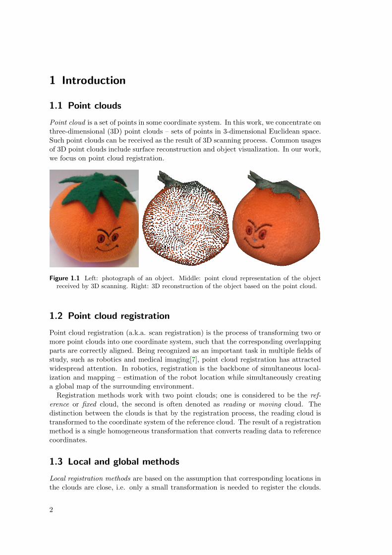
Point cloud is a set of points in some coordinate system. In this work, we concentrate onthree-dimensional (3D) point clouds – sets of points in 3-dimensional Euclidean space.Such point clouds can be received as the result of 3D scanning process. Common usagesof 3D point clouds include surface reconstruction and object visualization. In our work,we focus on point cloud registration.
Figure 1.1 Left: photograph of an object. Middle: point cloud representation of the objectreceived by 3D scanning. Right: 3D reconstruction of the object based on the point cloud.
1.2 Point cloud registration
Point cloud registration (a.k.a. scan registration) is the process of transforming two ormore point clouds into one coordinate system, such that the corresponding overlappingparts are correctly aligned. Being recognized as an important task in multiple fields ofstudy, such as robotics and medical imaging[7], point cloud registration has attractedwidespread attention. In robotics, registration is the backbone of simultaneous local-ization and mapping – estimation of the robot location while simultaneously creatinga global map of the surrounding environment.
Registration methods work with two point clouds; one is considered to be the ref-erence or fixed cloud, the second is often denoted as reading or moving cloud. Thedistinction between the clouds is that by the registration process, the reading cloud istransformed to the coordinate system of the reference cloud. The result of a registrationmethod is a single homogeneous transformation that converts reading data to referencecoordinates.
1.3 Local and global methods
Local registration methods are based on the assumption that corresponding locations inthe clouds are close, i.e. only a small transformation is needed to register the clouds.
2
1.4 Relation to the NIFTi and TRADR projects
When the relative rotation or translation of the clouds is too large, local methodswill likely fail to provide the correct result. In some applications, an initial guessof the transformation is available, enabling local methods to work with large clouddisplacements. This is frequently used in robotics – a transformation approximation isprovided by inertial navigation systems and wheel odometry. Concerning local methods,the contribution of our work is as follows: we test a number methods head-to-headon various difficult datasets. The results provide a clear comparison of the methods’precision and robustness to displacement (see chapter 2).
Global registration methods function independently of the original displacement of theclouds. Therefore, in contrast to local methods, large relative translation or rotationhas no effect on the result. Conventional global methods use geometrical informationto find corresponding locations in the clouds. Our work contributes to this field byproposing changes to global methods that take advantage of camera imagery, i.e. visualinformation (see chapter 3).
1.4 Relation to the NIFTi and TRADR projects
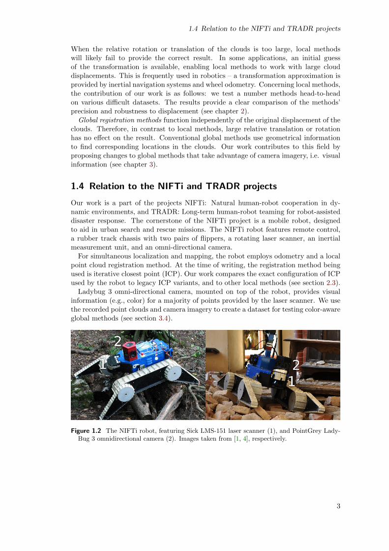
Our work is a part of the projects NIFTi: Natural human-robot cooperation in dy-namic environments, and TRADR: Long-term human-robot teaming for robot-assisteddisaster response. The cornerstone of the NIFTi project is a mobile robot, designedto aid in urban search and rescue missions. The NIFTi robot features remote control,a rubber track chassis with two pairs of flippers, a rotating laser scanner, an inertialmeasurement unit, and an omni-directional camera.
For simultaneous localization and mapping, the robot employs odometry and a localpoint cloud registration method. At the time of writing, the registration method beingused is iterative closest point (ICP). Our work compares the exact configuration of ICPused by the robot to legacy ICP variants, and to other local methods (see section 2.3).
Ladybug 3 omni-directional camera, mounted on top of the robot, provides visualinformation (e.g., color) for a majority of points provided by the laser scanner. We usethe recorded point clouds and camera imagery to create a dataset for testing color-awareglobal methods (see section 3.4).
Figure 1.2 The NIFTi robot, featuring Sick LMS-151 laser scanner (1), and PointGrey Lady-Bug 3 omnidirectional camera (2). Images taken from [1, 4], respectively.
3
2 Local methods
2.1 Related work
In this section we introduce the local methods that are subject to our experiments.
2.1.1 ICP: Iterative closest point
The iterative closest point (ICP) algorithm has been originally proposed by Chen andMedioni[11], and Besl and McKay[9]. Its simplicity and ease of implementation at-tracted significant attention. Since its inception in 1991, a large body of related workhas been created, counting over 400 papers in the past 20 years[21].
To briefly describe the algorithm: ICP iteratively improves the relative pose of twooverlapping point clouds. In each iteration, the following steps are performed:
1. For each point in the reading cloud, the closest point in the reference cloud is found.
2. A transformation of the reading cloud is determined, minimizing an objective func-tion. This is either the sum of squared distances between the corresponding points(point-to-point, as described by Besl and McKay[9]), or between a point from thereading cloud and the tangent plane of the corresponding point from the referencecloud (point-to-plane, as in Chen and Medioni[11]).
3. Found transformation is applied to the reading cloud. Tests for convergence (anddivergence) of the transformation are queried, possibly ending the loop.
Finding the closest point in the reference cloud for each of the points in the read-ing cloud has been identified as a performance bottleneck of the method, requiringacceleration by a fast search algorithm, such as kd-tree[12]. Additionally, various pre-processing steps are applied to the clouds, for example to remove redundant data, orto pre-compute surface normals for points in the reference cloud.
Due to the popularity of ICP, a great number of its variants have emerged. Toease the selection of a proper variant for a given task, Pomerleau et al. have createdthe libpointmatcher framework[21], enabling to create and compare customized ICPconfigurations. Kubelka et al.[15] have proposed one such configuration, which we usein our following experiments.
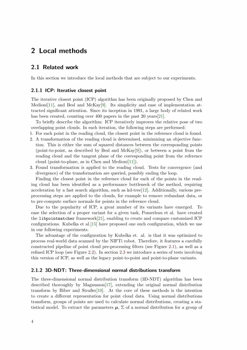
The advantage of the configuration by Kubelka et. al. is that it was optimized toprocess real-world data scanned by the NIFTi robot. Therefore, it features a carefullyconstructed pipeline of point cloud pre-processing filters (see Figure 2.1), as well as arefined ICP loop (see Figure 2.2). In section 2.3 we introduce a series of tests involvingthis version of ICP, as well as the legacy point-to-point and point-to-plane variants.
2.1.2 3D-NDT: Three-dimensional normal distributions transform
The three-dimensional normal distribution transform (3D-NDT) algorithm has beendescribed thoroughly by Magnusson[17], extending the original normal distributiontransform by Biber and Straßer[10]. At the core of these methods is the intentionto create a different representation for point cloud data. Using normal distributionstransform, groups of points are used to calculate normal distributions, creating a sta-tistical model. To extract the parameters µ, Σ of a normal distribution for a group of
4
2.1 Related work
SimpleSensorNoise
data position uncertainties calculated, based on sensor specifications
SamplingSurfaceNormal
calculates normals (using 20 nearest neighbors), keeping 80% of the points
ObservationDirection
calculates direction to the scanner
OrientNormals
re-orients normals towards the observation direction
MaxDensity
removes points to achieve maximum density of 100 points per cubic meter
Filters
Figure 2.1 Diagram of pre-processing filters used on input clouds by Kubelka et al.[15]
readingDataPointsFilters
Reading cloud preprocessing
referenceDataPointsFilters
Reference cloud preprocessing
matcher
Finds corresponding points in each cloud
outlierFilters
Discards correspondences based on some criteria
errorMinimizer
Finds the transformation that minimizes a given cost function
transformationCheckers
Ends the loop if any of the given conditions is met
KDTree - nearest point search up to 0.5 m,
ε = 3.16
Filters - as in the previous figure
KDTree - removes correspondence if
angle of normals > 50°
TrimmedDist - keeps 80 % closest
correspondences
Differential - reading cloud moved less than 0.01 m and 0.001 rad
Counter - 40 iterations elapsed
Bound - reading cloud further than 5 m and
0.8 rad from initial position
PointToPlane - minimize distance between point and correspond. tangent plane
ICP
Figure 2.2 Diagram of the ICP algorithm key steps, as implemented in the libpointmatcher
library[21] and configured by Kubelka et al.[15]
5
2 Local methods
A second issue is, that for a noise free measured world line, the covariancematrix will get singular and cannot be inverted. In practice, the covariance ma-trix can sometimes get near singular. To prevent this e�ect, we check, whetherthe smaller eigenvalue of � is at least 0:001 times the larger eigenvalue. If not,it is set to this value. This also has the e�ect of smoothing lines a little bit.
Figure 1 contains some example transformations of single cells. Shown arethe 2D points and the probability density. The visualization is created by eval-uating the probability density at each point, bright areas indicate high prob-ability densities. Figure 2 show some example transformations of whole laserscans. The next section shows, how this transformation is used to align twolaser scans.
Figure 1: The NDTs of some single cells.
5 Scan alignment
The spatial mapping T between two robot coordinate frames is given by
T :
�x0
y0
�=
�cos� � sin�sin� cos�
��xy
�+
�txty
�; (2)
where (tx; ty)t describes the translation and � the rotation between the two
frames. The goal of the scan alignment is to recover these parameters using thelaser scans taken at two positions. The outline of the proposed approach, giventwo scans (the �rst one and the second one), is as follows:
1. Build the Normal Distribution Transform of the �rst scan.
2. Initialize the estimate for the parameters (by zero or by using odometrydata).
6
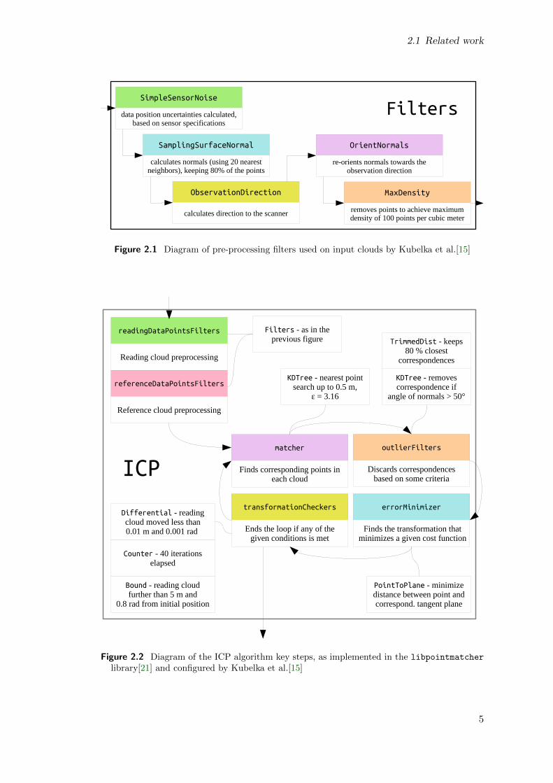
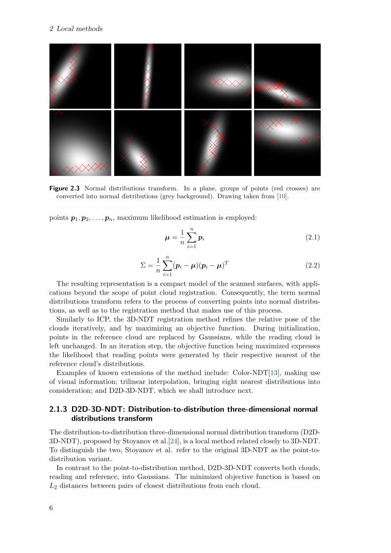
Figure 2.3 Normal distributions transform. In a plane, groups of points (red crosses) areconverted into normal distributions (grey background). Drawing taken from [10].
points p1,p2, . . . ,pn, maximum likelihood estimation is employed:
µ =1
n
n∑i=1
pi (2.1)
Σ =1
n
n∑i=1
(pi − µ)(pi − µ)T (2.2)
The resulting representation is a compact model of the scanned surfaces, with appli-cations beyond the scope of point cloud registration. Consequently, the term normaldistributions transform refers to the process of converting points into normal distribu-tions, as well as to the registration method that makes use of this process.
Similarly to ICP, the 3D-NDT registration method refines the relative pose of theclouds iteratively, and by maximizing an objective function. During initialization,points in the reference cloud are replaced by Gaussians, while the reading cloud isleft unchanged. In an iteration step, the objective function being maximized expressesthe likelihood that reading points were generated by their respective nearest of thereference cloud’s distributions.
Examples of known extensions of the method include: Color-NDT[13], making useof visual information; trilinear interpolation, bringing eight nearest distributions intoconsideration; and D2D-3D-NDT, which we shall introduce next.
The distribution-to-distribution three-dimensional normal distribution transform (D2D-3D-NDT), proposed by Stoyanov et al.[24], is a local method related closely to 3D-NDT.To distinguish the two, Stoyanov et al. refer to the original 3D-NDT as the point-to-distribution variant.
In contrast to the point-to-distribution method, D2D-3D-NDT converts both clouds,reading and reference, into Gaussians. The minimized objective function is based onL2 distances between pairs of closest distributions from each cloud.
6
2.2 Datasets
In the experiments presented by Stoyanov et al., the distribution-to-distribution ap-proach has shown promising results. Our work thoroughly compares this method to3D-NDT and others, providing an overview of its precision and robustness to initialdisplacement.
2.2 Datasets
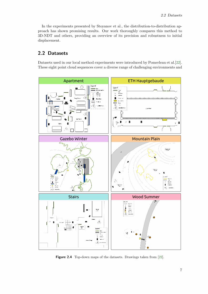
Datasets used in our local method experiments were introduced by Pomerleau et al.[22].These eight point cloud sequences cover a diverse range of challenging environments and
Apartment ETH Hauptgebaude
Gazebo Winter Mountain Plain
Stairs Wood Summer
Figure 2.4 Top-down maps of the datasets. Drawings taken from [22].
7
2 Local methods
situations, providing precise ground truth poses of the sensor measured by a theodolite(translation error under 1.8 mm, rotation error under 0.006 rad[22]). Hokuyo UTM-30LX laser scanner was used to capture the data, providing 100.000 to 350.000 pointsper scan. Let us describe the six sequences that we used in our experiments:
• Apartment – a sequence of point clouds in a single-floor apartment with five rooms: akitchen, a bathroom, an office and a bedroom. Such environment is well structured,i.e. most surfaces in the environment are representable by geometric primitives. Al-though some dynamic elements were created by purposely relocating objects betweenscans, the apartment sequence is considered the least difficult to register.
• ETH Hauptgebaude – point clouds in this sequence were scanned in a hallway, fea-turing repetitive elements, such as pillars and arches. This creates an interestingchallenge, as local registration methods tend to converge to the local minima of theirrespective cost function, which repetitive elements may create.
• Gazebo Winter – an outdoor, semi-structured dataset, with both geometrically simpleand complex surfaces. The point clouds were scanned near a summer house in a park,surrounded by trees. To further increase registration difficulty, people were recordedboth sitting and in motion – walking in the scene during the scanning process.
• Mountain Plain – an unstructured outdoor scene, featuring no man-made structuresand no obvious vertical landmarks. Covered in approximately 0.5 m tall grass, theplain has proven to be a substantially challenging scene for registration methods, asthere are no vertical surfaces to sufficiently constrain the registration process.
• Stairs – a dataset for testing methods’ robustness to large changes in scanned volumes,i.e. sizes of areas represented by a point cloud. In the sequence, starting indoors, thescanner first passes through a few doorways, eventually leaving the building into anoutdoor environment.
• Wood Summer – an outdoor scene, recorded in a forest. Apart from a small pavedroad, all objects in the scene (trees and other vegetation) consist of unstructuredsurfaces. Furthermore, as in the Gazebo Winter dataset, dynamic elements werecreated by recording people in motion.
Hand in hand with a dataset is a protocol – a pre-generated sequence of scan pairs toregister, along with initial guesses of the relative pose. In our experiments, we use twodifferent protocols for the above-mentioned datasets. On these protocols, we elaboratein detail in sections 2.3 and 2.4.
2.3 ETHZ protocol
First of the two protocols we used to test local methods is one proposed by Pomerleau etal.[21], from ETH Zurich, based on the datasets described in the previous section. Theprotocol features 35 pairs of clouds for each of the six datasets, with 192 initial posesfor each pair, totalling over 40,000 registrations. For a dataset, point cloud pairs havebeen selected so that their overlaps, i.e. the amount of represented surfaces that arecommon to both clouds, are distributed approximately uniformly from 30 % to 99 %.
Each protocol entry consists of a reading and a reference cloud, an initial transfor-mation for the reading cloud, and an expected resulting transformation TG (the groundtruth). To evaluate the protocol, the method in question is run on all the entries. Af-ter a method registers a pair of clouds, the resulting transformation TR is analyzed to
8
2.4 Our protocol
receive traslational error εt and rotational error εr:
∆T = TRT−1G =
[∆R ∆t0 1
](2.3)
εt = ‖∆t‖2 (2.4)
εr = arccos
(trace(∆R)− 1
2
)(2.5)
The above formula extracts the minimum distance (in meters) and minimum angle(in radians), by which the final pose TR is be moved to be identical to the ground truthpose TG. To compare method capabilities, we use three quantiles of rotational andtranslational errors:
A50 0.5-quantile, the median
A75 0.75-quantile
A95 0.95-quantile
Initial poses were artificially generated from the ground truth pose by offsetting it bya perturbation (i.e. displacement). Three perturbation types are used in this protocol,Easy, Medium and Hard, with increasing standard deviations of zero-mean Gaussians,from which samples were taken to generate the displacements. For each perturbationtype and point cloud pair, the protocol contains 64 initial poses.
We evaluate this protocol to explore the precision and robustness of three new meth-ods (ICP by Kubelka et al.[15], 3D-NDT, D2D-3D-NDT), in comparison to one anotherand to legacy ICP variants (see section 2.6 for an overview of the tested methods). Re-sults for the Easy perturbation type represent the situation where the method wasgiven a good initial pose; the lower the error for A50 and A75 quantiles, the betterthe precision of the method. On the other hand, low A95 quantiles are generally anindication of method robustness. Furthermore, results may vary greatly for differentdatasets, given their diverse nature (see section 2.2).
2.4 Our protocol
Although the ETHZ protocol is sufficient for basic method comparison, we chose to cre-ate our own protocol in order to explore the limitations of local registration methods.We suspect that methods are variously susceptible to the two types of initial displace-ment, translational and rotational, and their combinations. Therefore, we would like toinvestigate a larger number of perturbation types than the three of the ETHZ protocol.
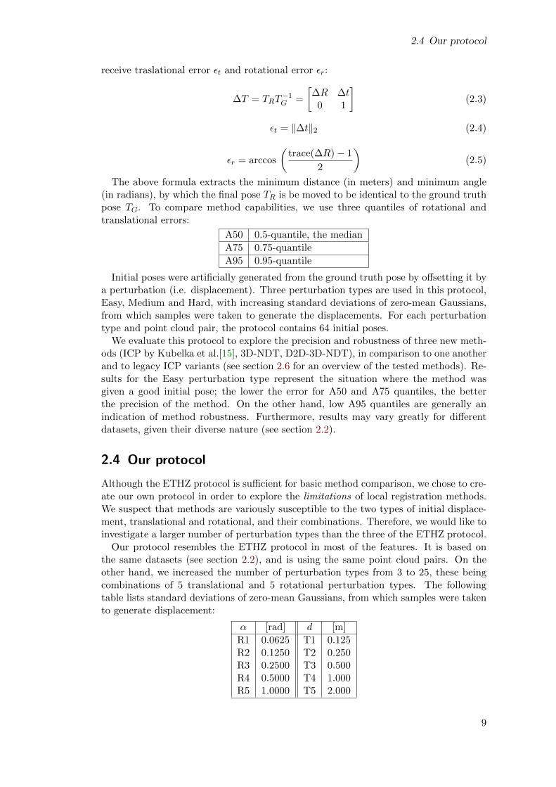
Our protocol resembles the ETHZ protocol in most of the features. It is based onthe same datasets (see section 2.2), and is using the same point cloud pairs. On theother hand, we increased the number of perturbation types from 3 to 25, these beingcombinations of 5 translational and 5 rotational perturbation types. The followingtable lists standard deviations of zero-mean Gaussians, from which samples were takento generate displacement:
To generate a protocol entry, given its perturbation type, an angle sample α and adistance sample d were taken from the corresponding distributions. To displace theground truth pose rotationally, we rotate it by α about a random axis; to performthe translational displacement, we translate it by d in a random direction. The final,perturbed pose is used as the initial pose for registration. As in the ETHZ dataset, 64initial poses were generated for each point cloud pair and perturbation type.
By evaluating this protocol, we push the tested methods to their limits, explor-ing their robustness to a large number of combinations of rotational and translationaldisplacements. This allows us to investigate the methods in unprecedented detail, over-coming any previous work on the matter. For all datasets, we find the limitations ofthe tested algorithms, i.e. our results indicate a maximum displacement for a methodto operate, given error requirements. Furthermore, by providing a detailed comparisonof the methods, the experimental results are a valuable resource for finding the bestalgorithm for a given environment and task.
2.5 Method composition
Intuitively, a method that is generally robust to initial displacement can be composedwith a precise method to form a new, composite method that is potentially superior toits parts. Our initial experiments with the ETHZ protocol (these experimental resultsare demonstrated in section 2.7.1) suggested that while D2D-3D-NDT falls short toICP and 3D-NDT in terms of robustness, its capabilities of precise registration weremore than satisfactory. Therefore, we decided to compose D2D-3D-NDT as the backend to ICP and 3D-NDT, creating two chained methods. In order to investigate thefeasibility of these methods, we tested them using both experimental protocols. Theresults are shown in sections 2.7.1 and 2.7.2.
2.6 Overview of tested methods
Here we provide a summary of the tested methods.
• Besl ICP, Chen ICP – legacy point-to-point and point-to-plane ICP methods, asdescribed by Besl and McKay[9] and Chen and Medioni[11]. Evaluated results ofthese methods were provided by Pomerleau et. al.[21]. ICP is discussed in detail insection 2.1.1. In our experiments, these legacy methods establish a baseline to whichone can compare the following new algorithms.
• ICP – an ICP configuration by Kubelka et al.[15]. We describe the algorithm indiagram 2.2. As an example of a configuration refined on a real-world registrationapplication, we anticipate its capabilities to be of the best currently attainable by avariant of ICP.
• P2D – an implementation of 3D-NDT from the PCL library, publicly available at[5]. The reading cloud is filtered as in the ICP method (see diagram 2.1). For moreinformation on 3D-NDT, see section 2.1.2.
• D2D – an implementation of the D2D-3D-NDT method provided by Center for Ap-plied Autonomous Sensor Systems at Orebro University, Sweden, publicly availableat http://code.google.com/p/oru-ros-pkg/. We describe this method in sec-tion 2.1.3.
• ICP-D2D, P2D-D2D – composite methods. We explain our motivation to includethese methods in section 2.5.
10
2.7 Experimental results
2.7 Experimental results
2.7.1 ETHZ protocol
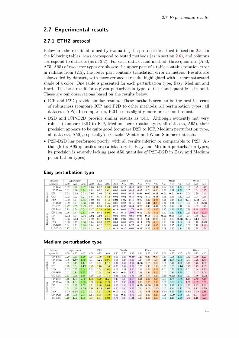
Below are the results obtained by evaluating the protocol described in section 2.3. Inthe following tables, rows correspond to tested methods (as in section 2.6), and columnscorrespond to datasets (as in 2.2). For each dataset and method, three quantiles (A50,A75, A95) of two error types are shown; the upper part of a table contains rotation errorin radians from (2.5), the lower part contains translation error in meters. Results arecolor-coded by dataset, with more erroneous results highlighted with a more saturatedshade of a color. One table is presented for each perturbation type, Easy, Medium andHard. The best result for a given perturbation type, dataset and quantile is in bold.These are our observations based on the results below:
• ICP and P2D provide similar results. These methods seem to be the best in termsof robustness (compare ICP and P2D to other methods, all perturbation types, alldatasets, A95). In comparison, P2D seems slightly more precise and robust.
• D2D and ICP-D2D provide similar results as well. Although evidently not veryrobust (compare D2D to ICP, Medium perturbation type, all datasets, A95), theirprecision appears to be quite good (compare D2D to ICP, Medium perturbation type,all datasets, A50), especially on Gazebo Winter and Wood Summer datasets.
• P2D-D2D has performed poorly, with all results inferior or comparable to P2D. Al-though its A95 quantiles are satisfactory in Easy and Medium perturbation types,its precision is severely lacking (see A50 quantiles of P2D-D2D in Easy and Mediumperturbation types).
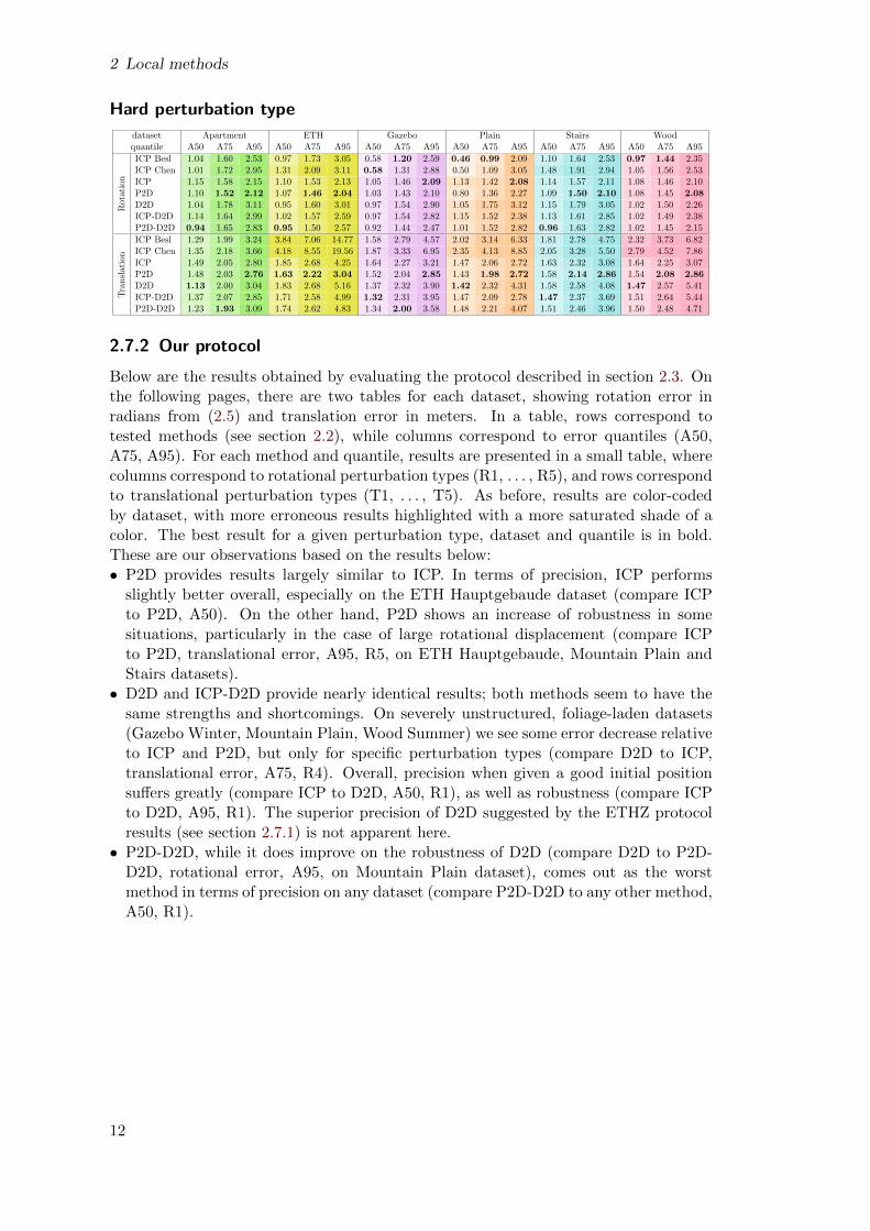
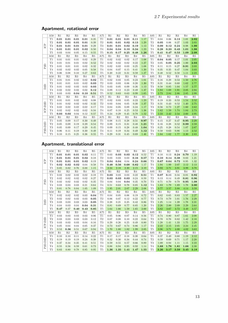
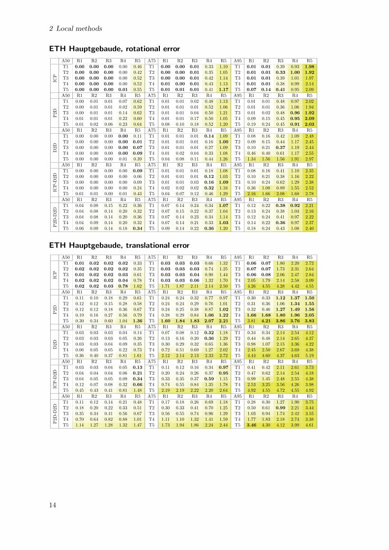
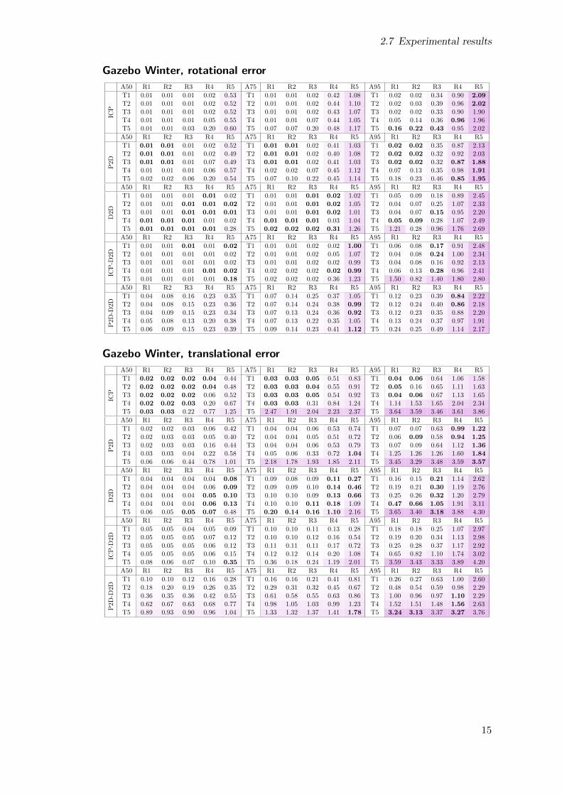
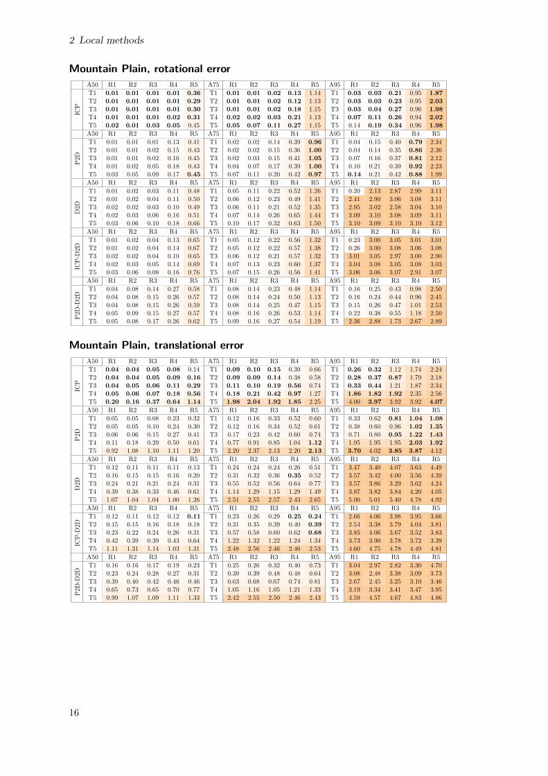
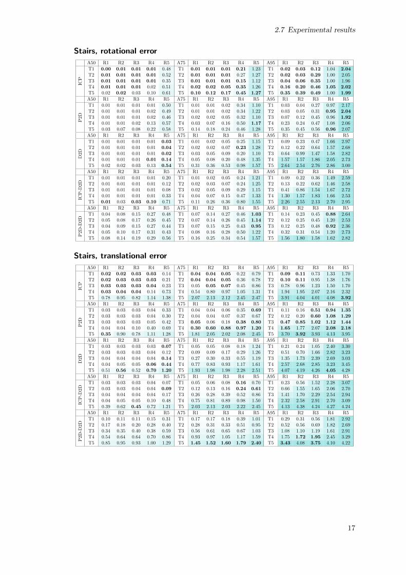
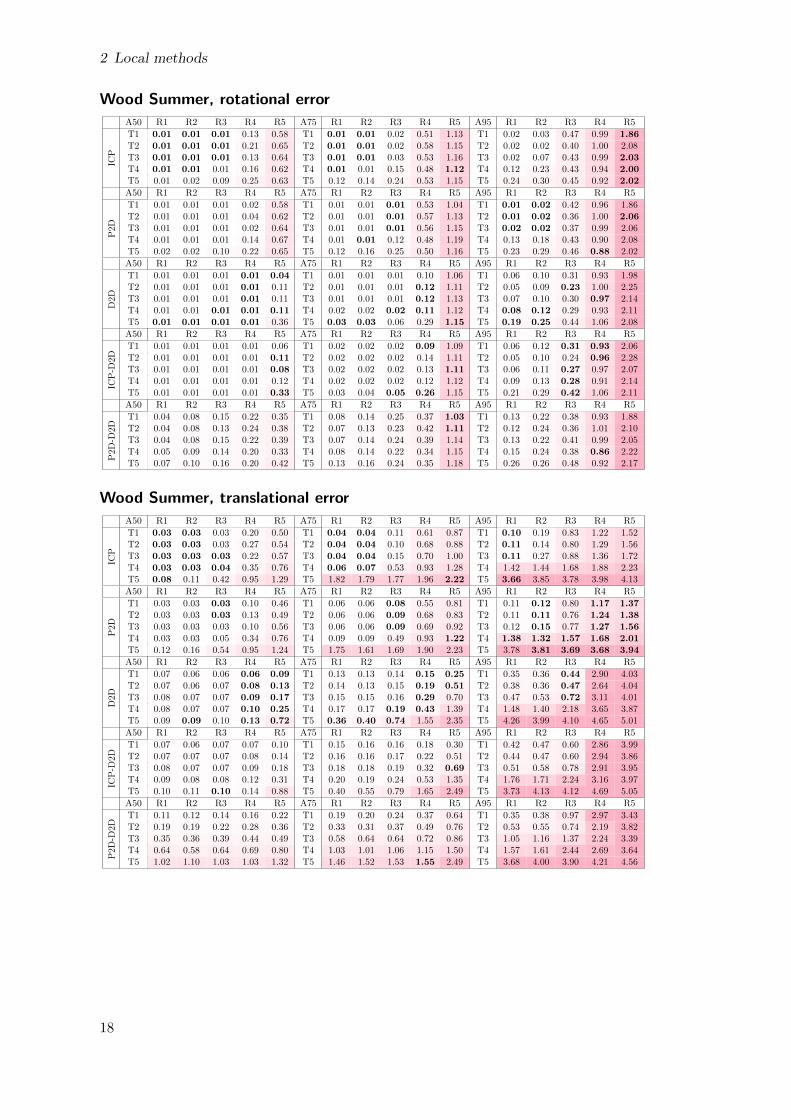
Below are the results obtained by evaluating the protocol described in section 2.3. Onthe following pages, there are two tables for each dataset, showing rotation error inradians from (2.5) and translation error in meters. In a table, rows correspond totested methods (see section 2.2), while columns correspond to error quantiles (A50,A75, A95). For each method and quantile, results are presented in a small table, wherecolumns correspond to rotational perturbation types (R1, . . . , R5), and rows correspondto translational perturbation types (T1, . . . , T5). As before, results are color-codedby dataset, with more erroneous results highlighted with a more saturated shade of acolor. The best result for a given perturbation type, dataset and quantile is in bold.These are our observations based on the results below:• P2D provides results largely similar to ICP. In terms of precision, ICP performs
slightly better overall, especially on the ETH Hauptgebaude dataset (compare ICPto P2D, A50). On the other hand, P2D shows an increase of robustness in somesituations, particularly in the case of large rotational displacement (compare ICPto P2D, translational error, A95, R5, on ETH Hauptgebaude, Mountain Plain andStairs datasets).• D2D and ICP-D2D provide nearly identical results; both methods seem to have the
same strengths and shortcomings. On severely unstructured, foliage-laden datasets(Gazebo Winter, Mountain Plain, Wood Summer) we see some error decrease relativeto ICP and P2D, but only for specific perturbation types (compare D2D to ICP,translational error, A75, R4). Overall, precision when given a good initial positionsuffers greatly (compare ICP to D2D, A50, R1), as well as robustness (compare ICPto D2D, A95, R1). The superior precision of D2D suggested by the ETHZ protocolresults (see section 2.7.1) is not apparent here.• P2D-D2D, while it does improve on the robustness of D2D (compare D2D to P2D-
D2D, rotational error, A95, on Mountain Plain dataset), comes out as the worstmethod in terms of precision on any dataset (compare P2D-D2D to any other method,A50, R1).
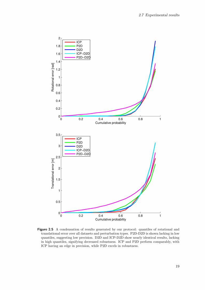
Figure 2.5 A condensation of results generated by our protocol: quantiles of rotational andtranslational error over all datasets and perturbation types. P2D-D2D is shown lacking in lowquantiles, suggesting low precision. D2D and ICP-D2D show nearly identical results, lackingin high quantiles, signifying decreased robustness. ICP and P2D perform comparably, withICP having an edge in precision, while P2D excels in robustness.
19
2 Local methods
2.8 Conclusion
Using a custom, detailed protocol based on well-established datasets, we provide an un-precedented level of insight into precision and robustness of local methods, overcomingany previous work that we know of.
Analysis of our data provides information that simplifies selection of the best methodfor a given environment. Specifically, our results suggest an overall dominance of theICP method configured by Kubelka et al.[15], and the Point Cloud Library implementa-tion of the 3D-NDT (P2D) method. On any of the diverse set of datasets, one of thesetwo methods provides the best results, both robustness- and precision-wise. Therefore,we suggest these methods to be the first choice for a 3D point cloud registration task.
Furthermore, using our results, one can find the limitations of any of the testedmethods. Given error requirements, one can identify a maximum displacement that themethod can overcome in a specific environment. This gives a clear picture of a method’scapabilities with chosen constraints on translational and rotational error. Additionally,when evaluated using our protocol, any other algorithms and configurations can bethoroughly compared to the methods included in our experiments.
Needless to say, susceptibility to displacement of the initial pose is a fundamentallimitation of all local methods. To perform registration with an arbitrary initial pose,a global method is needed.
20
3 Global methods
In contrast to local methods, global registration methods function independently of theinitial relative pose of the clouds. Consequently, no initial guess of the relative poseis needed, as cloud displacement has no effect on the result. In our work, we focus onfeature-based global registration methods. By features we mean descriptions of localpoint cloud data, which can be extracted and matched with each other. Features arecreated at keypoints, i.e. points of interest in a cloud. The core problem of feature-basedregistration is the maximization of repeatability – the same keypoints and features areto be found in different point clouds. Repeatability enables us to find correspondingfeatures in the reading and reference clouds, which we use to estimate the relative pose.
3.1 Related work
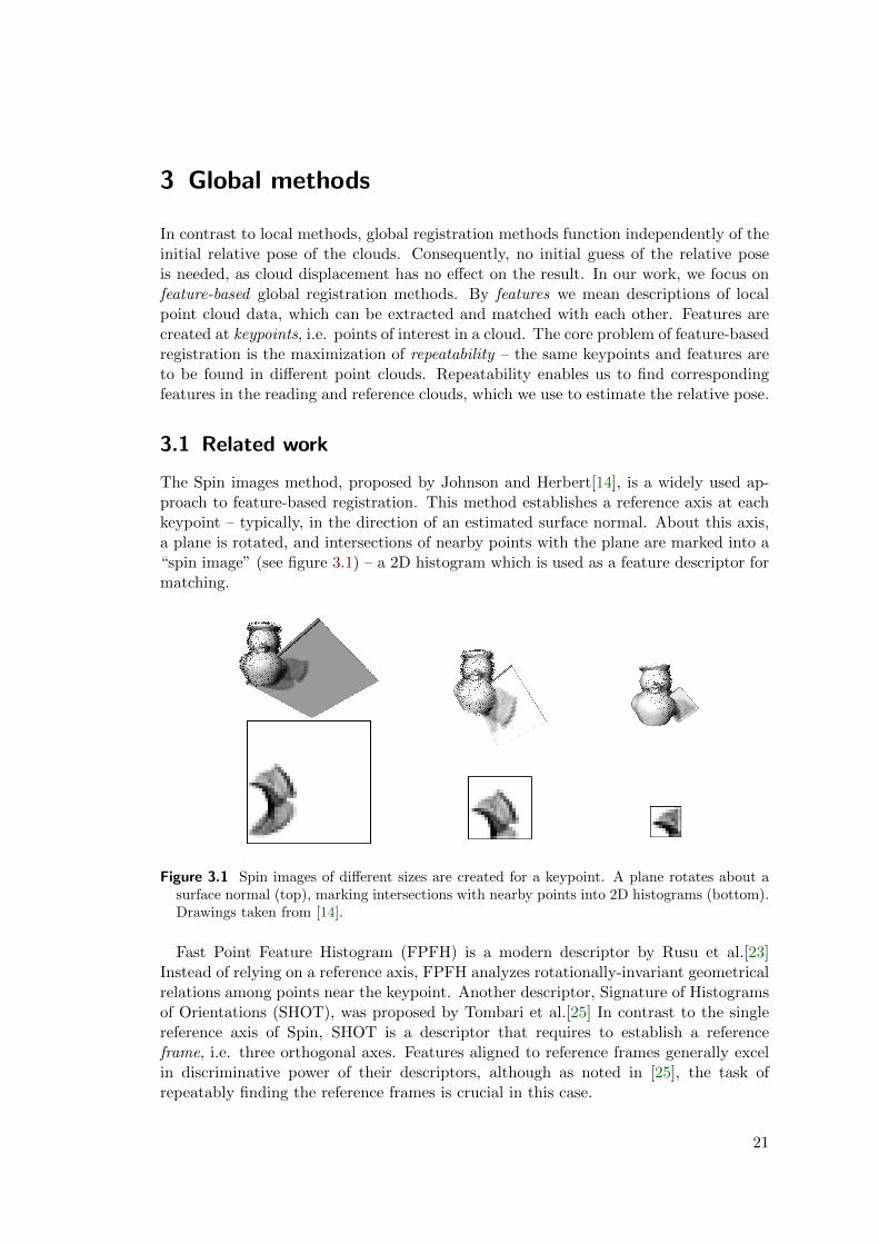
The Spin images method, proposed by Johnson and Herbert[14], is a widely used ap-proach to feature-based registration. This method establishes a reference axis at eachkeypoint – typically, in the direction of an estimated surface normal. About this axis,a plane is rotated, and intersections of nearby points with the plane are marked into a“spin image” (see figure 3.1) – a 2D histogram which is used as a feature descriptor formatching.JOHNSON AND HEBERT: USING SPIN IMAGES FOR EFFICIENT OBJECT RECOGNITION IN CLUTTERED 3D SCENES 437
Although spin images can have any number of rows andcolumns, for simplicity, we generally make the number ofrows and columns in a spin image equal. This results insquare spin images whose size can be described by one pa-rameter. We define the number of rows or columns in asquare spin image to be the image width. To create a spinimage, an appropriate image width needs to be determined.Image width times the bin size is called the spin image sup-port distance (Ds); support distance determines the amountof space swept out by a spin image. By setting the imagewidth, the amount of global information in a spin imagecan be controlled. For a fixed bin size, decreasing imagewidth will decrease the descriptiveness of a spin image be-cause the amount of global shape included in the imagewill be reduced. However, decreasing image width will alsoreduce the chances of clutter corrupting a spin image. Im-age width is analogous to window size in 2D templatematching. Fig. 4 shows spin images for a single orientedpoint on the duck model as the image width is decreased.This figure shows that as image width decreases, the de-scriptiveness of the images decreases.
The graph in the middle of Fig. 6 shows the effect of im-age width on spin image matching. As image width de-creases, match distance decreases. This confirms our obser-vation from Fig. 4. In general, we set the image width sothat the support distance is on order of the size of themodel. If the data is very cluttered, then we set the imagewidth to a smaller value. For the results presented in this
paper, image width is set to 15, resulting in spin imageswith 225 bins.
The final spin image generation parameter is support an-gle (As). Support angle is the maximum angle between thedirection of the oriented point basis of a spin image and thesurface normal of points that are allowed to contribute tothe spin image. Suppose we have an oriented point $ with
position and normal (p$, n$) for which we are creating aspin image. Furthermore, suppose there exists another ori-ented point % with position and normal (p%, n%). The sup-port angle constraint can then be stated as: % will be accu-mulated in the spin image of $ if
acos(n$ ¼ n%) < As.
Support angle is used to limit the effect of self occlusionand clutter during spin image matching. Fig. 5 shows thespin image generated for three different support anglesalong with the vertices on the model that are mapped intothe spin image. Support angle is used to reduce the numberof points on the opposite side of the model that contributeto the model spin image. This parameter decreases the ef-fect of occlusion on spin image matching; if a point has sig-nificantly different normal from the normal of the orientedpoint, then it is unlikely that it will be visible when the ori-ented point is imaged by a rangefinder in some scene data.
Decreasing support angle also has the effect of decreas-
Fig. 4. The effect of image width on spin images. As image width decreases, the volume swept out by the spin image (top) decreases, resulting indecreased spin image support (bottom). By varying the image width, spin images can vary smoothly from global to local representations. (a) A 40-pixel image width. (b) A 20-pixel image width. (c) A 10-pixel image width.
Fig. 5. The effect of support angle on spin image appearance. As support angle decreases, the number of points contributing to the spin image(top) decreases. This results in reduction in the support of the spin images (bottom). (a) A 180 degree support angle. (b) A 90 degree supportangle. (c) A 60 degree support angle.
Figure 3.1 Spin images of different sizes are created for a keypoint. A plane rotates about asurface normal (top), marking intersections with nearby points into 2D histograms (bottom).Drawings taken from [14].
Fast Point Feature Histogram (FPFH) is a modern descriptor by Rusu et al.[23]Instead of relying on a reference axis, FPFH analyzes rotationally-invariant geometricalrelations among points near the keypoint. Another descriptor, Signature of Histogramsof Orientations (SHOT), was proposed by Tombari et al.[25] In contrast to the singlereference axis of Spin, SHOT is a descriptor that requires to establish a referenceframe, i.e. three orthogonal axes. Features aligned to reference frames generally excelin discriminative power of their descriptors, although as noted in [25], the task ofrepeatably finding the reference frames is crucial in this case.
21
3 Global methods
The feature-based method by Petricek and Svoboda[19] also employs a referenceframe-based descriptor[20]. Our work is an extension of [19], proposing changes to itsdescriptor and reference frame determination that take advantage of visual information.A large body of work has been created on the topic of feature-based image registration,based solely on visual data. Prominent methods in this area include Scale InvariantFeature Transform (SIFT) by Lowe and David[16] and Speeded Up Robust Features(SURF) by Bay et al.[8] Binary Robust Appearance and Normals Descriptor (BRAND)by Nascimento et al.[18] is an example of a descriptor that fuses range and visual data,taking depth information from RGB-D images into consideration.
3.2 Overview of a feature-based method
In this section, we describe the key steps of a feature-based registration algorithm.Additionally, we discuss the specific implementations of these steps in the method byPetricek and Svoboda[19] that we propose modifications to in section 3.3.
3.2.1 Pre-processing
As in local methods (e.g. see figure 2.1), a sequence of filters is first applied to each ofthe clouds being registered to remove redundant and errorneous data, and to calculateadditional properties of points. Most feature-based methods suffer from non-uniformsampling density [14, 25, 19], requiring a density filter, and many methods also makeuse of surface normals calculated for each point in pre-processing [23, 25, 19].
3.2.2 Keypoint detection
Determining the locations of features is accomplished by defining a saliency measure,i.e. a measure of interest in a given location. Each point in a cloud is treated as akeypoint candidate; the saliency measure is calculated at the position of every point,and points that produce local maxima of the measure are then promoted to keypoints.To calculate the measure in [19] for a given point, nearby points pi are found up to thedistance of 0.35 m. Then, the covariance matrix C of point positions is found:
µ =
∑i pi∑i 1
(3.1)
C =∑i
(pi − µ)(pi − µ)T (3.2)
As C is a positive semidefinite matrix with real coefficients, singular value decom-position (SVD) of C yields real positive eigenvalues λ1 > λ2 > λ3 and correspondingorthonormal eigenvectors v1, v2, v3:
C = USV T = V SV T =[v1 v2 v3
] λ1 0 00 λ2 00 0 λ3
vT1vT2vT3
(3.3)
In [19], it is shown that λ3 is a good choice of a saliency measure; flat surfacesare given a low saliency score in favor of edges and corners. Finally, non-maximumsuppression is used to find the local maxima – a keypoint candidate is discarded ifthere is a more salient point in a 0.2 m radius. Remaining candidates form keypointsat the mean positions µ from equation 3.1.
22
3.2 Overview of a feature-based method
3.2.3 Reference frame determination and disambiguation
This step is performed only for methods that require a reference frame to align their de-scriptor [25, 20]; some descriptors require only a single reference axis[14] or no referenceaxes at all[23]. Tombari et al.[25] stress the importance of repeatable determination ofreference frames, which they believe is underrated in favor of descriptor choice.
To determine the reference frame of a given keypoint, Petricek and Svoboda[19] takethe principal components of positions of nearby points found within a radius of 2 m.A covariance matrix C is created from these points (as in equations 3.1, 3.2) and SVDapplied (as in 3.3) – eigenvectors v1, v2, v3 then form principal components, with v1in the direction of the largest position variance, and v3 in the direction of the lowest.
Directions of eigenvectors of the point covariance matrix are repeatable and widelyused as the reference frame of a keypoint [25, 19]; unfortunately, their signs are deter-mined accidentally by the SVD, creating four ambiguous rotation possibilites. Somefeature-based methods alleviate the problem by extracting multiple descriptors for akeypoint, one for each of the ambiguous reference frames. Tombari et al.[25] insteadpropose a sign disambiguation method, improving the repeatability of the signs. Thesign disambiguation method by Petricek and Svoboda[19] forces the orientation of twoaxes towards the position of the scanner. Given eigenvectors v1, v2, v3, a keypointlocation µ, and a scanner location s, the reference frame a1, a2, a3 is calculated asfollows:
In [19], it is noted that a3 provides a very repeatable direction, including the sign.With v3 being the direction of the lowest variance of positions, it is an estimation ofthe direction of the surface normal. All visible surfaces are inherently oriented towardsthe scanner; consequently, the sign disambiguation method based on sensor locationconsistently enforces the correct orientation of a3. On the other hand, the directions ofv1, v2 are not as stable, susceptible to missing parts of the surface (due to occlusion)and to non-uniform sampling density. To create a right-handed coordinate system, a1is calculated as the cross product of a2 and a3.
3.2.4 Descriptor extraction
The feature descriptor is an essential part of any feature-based method. Descriptors aredesigned to strike the balance between discriminative power and descriptor size, whichaffects memory requirements and performance. Most methods employ a histogram astheir descriptor [14, 23, 25, 19], while some rely on a binary string [18].
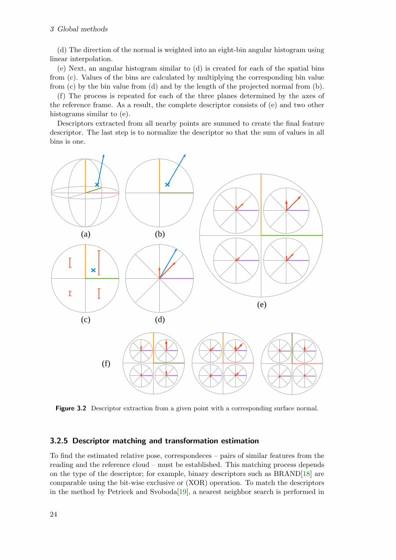
In [19], Petricek and Svoboda use a histogram of point positions and normal directionsas proposed in [20]. To extract the descriptor, nearby points up to the distance of 2 mare considered, along with their corresponding pre-calculated normals. Let us describethe process of marking a given point into the histogram (see figure 3.2).
(a) A point with a corresponding normal is located near the keypoint.
(b) Both the point and its normal are orthogonally projected onto one of the threeplanes determined by the axes of the reference frame.
(c) The position of the point is weighted into a four-bin spatial histogram using linearinterpolation.
23
3 Global methods
(d) The direction of the normal is weighted into an eight-bin angular histogram usinglinear interpolation.
(e) Next, an angular histogram similar to (d) is created for each of the spatial binsfrom (c). Values of the bins are calculated by multiplying the corresponding bin valuefrom (c) by the bin value from (d) and by the length of the projected normal from (b).
(f) The process is repeated for each of the three planes determined by the axes ofthe reference frame. As a result, the complete descriptor consists of (e) and two otherhistograms similar to (e).
Descriptors extracted from all nearby points are summed to create the final featuredescriptor. The last step is to normalize the descriptor so that the sum of values in allbins is one.
(a) (b)
(d)(c)
(e)
(f)
Figure 3.2 Descriptor extraction from a given point with a corresponding surface normal.
3.2.5 Descriptor matching and transformation estimation
To find the estimated relative pose, correspondeces – pairs of similar features from thereading and the reference cloud – must be established. This matching process dependson the type of the descriptor; for example, binary descriptors such as BRAND[18] arecomparable using the bit-wise exclusive or (XOR) operation. To match the descriptorsin the method by Petricek and Svoboda[19], a nearest neighbor search is performed in
24
3.3 Using camera imagery in feature-based registration
a high-dimensional space. Each bin of the histogram is treated as a dimension, andthe “distance” (i.e. dissimilarity) between two descriptors is measured by Euclideandistance. Based on the established descriptor pairs, a robust estimator is used toextract the approximate relative transformation. In [19], the RANSAC algorithm isemployed.
3.3 Using camera imagery in feature-based registration
3.3.1 Camera projection and 3D gradient direction
In our work, we propose changes to the method by Petricek and Svoboda[19] that makeuse of visual information available for the NIFTi robot. In particular, we take advantageof camera imagery captured during the scanning process. Since the camera calibrationdata is available for each video feed, it is possible to project a 3D point into any of thecamera images. We implemented a camera projection in MATLAB that complies withthe pinhole camera model with two tangential and three radial distortion coefficients[3].The following computation provides a camera projection (x′, y′) for a given 3D point(x, y, z): x1y1
z1
= R
xyz
+ t (3.6)
x2 = x1z1
y2 = y1z1
(3.7)
r = x22 + y22 (3.8)
x3 = x2(1 + k1r2 + k2r
4 + k3r6) + 2p1x2y2 + p2(r
2 + 2x22)y3 = y2(1 + k1r
2 + k2r4 + k3r
6) + 2p2x2y2 + p1(r2 + 2y22)
(3.9)
x′ = fxx3 + cx y′ = fyy3 + cy (3.10)
where fx, fy, cx, cy are intrinsic camera parameters, p1, p2 are tangential distortionparameters, and k1, k2, k3 are radial distortion parameters. The 3-by-3 rotation matrixR and translation vector t transform the point from world coordinates into a coordinatesystem fixed with respect to the camera, whose origin is at the center of the cameraprojection plane, its Z-axis is the view direction, its Y-axis is vertical and its X-axis ishorizontal.
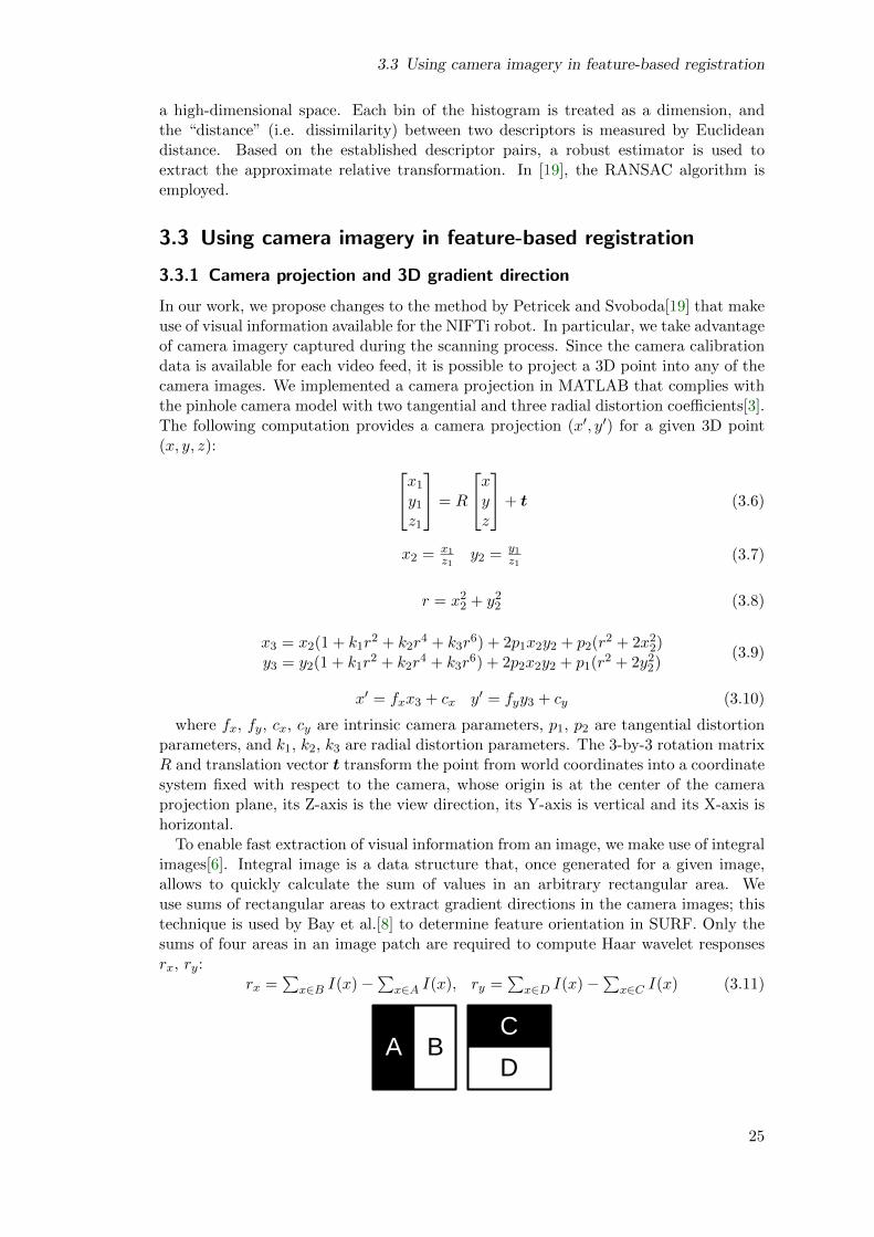
To enable fast extraction of visual information from an image, we make use of integralimages[6]. Integral image is a data structure that, once generated for a given image,allows to quickly calculate the sum of values in an arbitrary rectangular area. Weuse sums of rectangular areas to extract gradient directions in the camera images; thistechnique is used by Bay et al.[8] to determine feature orientation in SURF. Only thesums of four areas in an image patch are required to compute Haar wavelet responsesrx, ry:
rx =∑
x∈B I(x)−∑
x∈A I(x), ry =∑
x∈D I(x)−∑
x∈C I(x) (3.11)
D
CA B
25
3 Global methods
The resulting response vector (rx, ry) serves as an estimation of the dominant gradientdirection in the image patch. With good lighting conditions, the dominant directionis repeatable when viewed from different viewpoints; this motivates the usage of Haarwavelet responses in SURF[8]. We propose to use this technique to estimate a three-dimensional gradient direction for a given point with a specified surface normal. Ourmethod consists of the following steps:
1. First, we project the point in question into the camera images. Since we are consid-ering multiple camera views, we choose the best image for the point, based on thedistance of the projection to the nearest edge of the image.
2. In the best image, we consider a square image patch centered at the projection ofthe point. For this patch, we extract the dominant gradient direction as in equation3.11. We receive the two-dimensional response vector (rx, ry).
3. Using the 3-by-3 rotation matrix from equation 3.6, we transform the response vectorinto world coordinates:
r1 = R−1
rxry0
(3.12)
4. We assume that while the direction of the gradient is oriented as it appears from theviewpoint of the camera, the gradient is also tangential to the surface. Using thesurface normal n, we project the response vector (rx, ry) along the camera Z-axisonto the tangent plane of the point:
z = R−1
001
(3.13)
r2 = (r1 × z)× n (3.14)
5. To obtain the final gradient r, we normalize r2:
r =r2‖r2‖2
(3.15)
3.3.2 Descriptor extraction
Our goal is to extend the descriptor from section 3.2.4 using the available visual data.We propose to enhance the discriminative power of the descriptor by considering theabove mentioned 3D gradient directions. We modify two steps of the algorithm byPetricek and Svoboda[19]:
1. In pre-processing, we add a step to the end of the filtering pipeline that calculates the3D gradient direction for each point in the point cloud. To achieve scale invariance,we determine the sizes of image patches based on the distance to the camera; foreach point (x, y, z), we also find a point (u, v, w) translated in a direction orthogonalto the direction of the camera:uv
w
=
xyz
+ s ·R−11
00
(3.16)
where R is the rotation matrix from (3.6) and s is the intended size of the patch.Both the original and the translated 3D point are projected and their image distancedetermines the projected size of the patch s′:
s′ = ‖(x′, y′)− (u′, v′)‖2 (3.17)
26
3.3 Using camera imagery in feature-based registration
Keypoint detection
Feature MatchingTransformation
Estimation
pointsnormals keypoint locations
keypoint reference framesfeature descriptors
corresponding feature pairs
estimated relative pose
point clouds
scanner location
Reference Frame Determination
gradients
imagescamera
calibration
Descriptor Extraction
Pre-processing
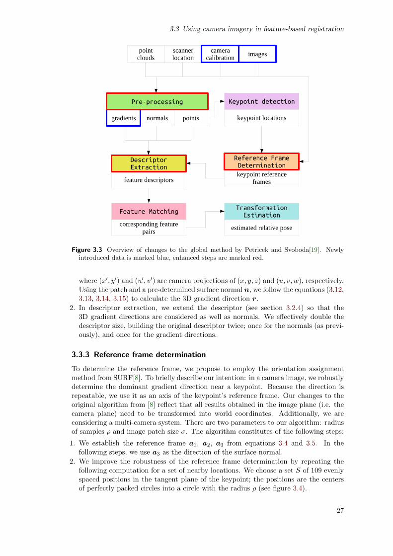
Figure 3.3 Overview of changes to the global method by Petricek and Svoboda[19]. Newlyintroduced data is marked blue, enhanced steps are marked red.
where (x′, y′) and (u′, v′) are camera projections of (x, y, z) and (u, v, w), respectively.Using the patch and a pre-determined surface normal n, we follow the equations (3.12,3.13, 3.14, 3.15) to calculate the 3D gradient direction r.
2. In descriptor extraction, we extend the descriptor (see section 3.2.4) so that the3D gradient directions are considered as well as normals. We effectively double thedescriptor size, building the original descriptor twice; once for the normals (as previ-ously), and once for the gradient directions.
3.3.3 Reference frame determination
To determine the reference frame, we propose to employ the orientation assignmentmethod from SURF[8]. To briefly describe our intention: in a camera image, we robustlydetermine the dominant gradient direction near a keypoint. Because the direction isrepeatable, we use it as an axis of the keypoint’s reference frame. Our changes to theoriginal algorithm from [8] reflect that all results obtained in the image plane (i.e. thecamera plane) need to be transformed into world coordinates. Additionally, we areconsidering a multi-camera system. There are two parameters to our algorithm: radiusof samples ρ and image patch size σ. The algorithm constitutes of the following steps:
1. We establish the reference frame a1, a2, a3 from equations 3.4 and 3.5. In thefollowing steps, we use a3 as the direction of the surface normal.
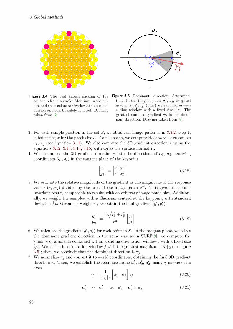
2. We improve the robustness of the reference frame determination by repeating thefollowing computation for a set of nearby locations. We choose a set S of 109 evenlyspaced positions in the tangent plane of the keypoint; the positions are the centersof perfectly packed circles into a circle with the radius ρ (see figure 3.4).
27
3 Global methods
N = 109109 circles in a circle
radius = 0.086489335895ratio = 11.562119071074
density = 0.815364169374contacts = 252
E.SPECHT23-APR-2010
N = 110110 circles in a circle
radius = 0.086081769648ratio = 11.616861550295
density = 0.815107817222contacts = 221
E.SPECHT21-MAR-2012
N = 111111 circles in a circle
radius = 0.085742621070ratio = 11.662811184493
density = 0.816049474538contacts = 220
E.SPECHT23-APR-2010
N = 112112 circles in a circle
radius = 0.085431571702ratio = 11.705274526430
density = 0.817437985675contacts = 215
E.SPECHT23-APR-2010
N = 113113 circles in a circle
radius = 0.085124290793ratio = 11.747528122480
density = 0.818814371785contacts = 220
E.SPECHT23-APR-2010
N = 114114 circles in a circle
radius = 0.084780441045ratio = 11.795173364030
density = 0.819400442944contacts = 215
E.SPECHT23-APR-2010
N = 115115 circles in a circle
radius = 0.084463211728ratio = 11.839474009347
density = 0.820413925573contacts = 226
E.SPECHT23-APR-2010
N = 116116 circles in a circle
radius = 0.084056891551ratio = 11.896704500333
density = 0.819605077999contacts = 215
E.SPECHT23-APR-2010
N = 117117 circles in a circle
radius = 0.083727722049ratio = 11.943475536278
density = 0.820208778422contacts = 221
E.SPECHT23-APR-2010
N = 118118 circles in a circle
radius = 0.083433794252ratio = 11.985551046315
density = 0.821421366756contacts = 217
E.SPECHT23-APR-2010
N = 119119 circles in a circle
radius = 0.083040377649ratio = 12.042334443872
density = 0.820588814099contacts = 233
E.SPECHT23-APR-2010
N = 120120 circles in a circle
radius = 0.082745752573ratio = 12.085212459928
density = 0.821623148262contacts = 231
E.SPECHT23-APR-2010
Figure 3.4 The best known packing of 109equal circles in a circle. Markings in the cir-cles and their colors are irrelevant to our dis-cussion and can be safely ignored. Drawingtaken from [2].
Figure 3.5 Dominant direction determina-tion. In the tangent plane a1, a2, weightedgradients (g′1, g
′2) (blue) are summed in each
sliding window with a fixed size 13π. The
greatest summed gradient γj is the domi-nant direction. Drawing taken from [8].
3. For each sample position in the set S, we obtain an image patch as in 3.3.2, step 1,substituting σ for the patch size s. For the patch, we compute Haar wavelet responsesrx, ry (see equation 3.11). We also compute the 3D gradient direction r using theequations 3.12, 3.13, 3.14, 3.15, with a3 as the surface normal n.
4. We decompose the 3D gradient direction r into the directions of a1, a2, receivingcoordinates (g1, g2) in the tangent plane of the keypoint.[
g1g2
]=
[rTa1rTa2
](3.18)
5. We estimate the relative magnitude of the gradient as the magnitude of the responsevector (rx, ry) divided by the area of the image patch s′2. This gives us a scale-invariant result, comparable to results with an arbitrary image patch size. Addition-ally, we weight the samples with a Gaussian centred at the keypoint, with standarddeviation 1
2ρ. Given the weight w, we obtain the final gradient (g′1, g′2):
[g′1g′2
]=w√r2x + r2y
s′2
[g1g2
](3.19)
6. We calculate the gradient (g′1, g′2) for each point in S. In the tangent plane, we select
the dominant gradient direction in the same way as in SURF[8]; we compute thesums γi of gradients contained within a sliding orientation window i with a fixed size13π. We select the orientation window j with the greatest magnitude ‖γj‖2 (see figure3.5); then, we conclude that the dominant direction is γj .
7. We normalize γj and convert it to world coordinates, obtaining the final 3D gradientdirection γ. Then, we establish the reference frame a′1, a
′2, a
′3, using γ as one of its
axes:
γ =1
‖γj‖2
[a1 a2
]γj (3.20)
a′2 = γ a′3 = a3 a′1 = a′2 × a′3 (3.21)
28
3.4 Dataset
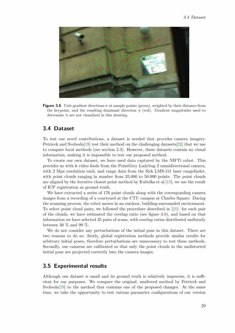
Figure 3.6 Unit gradient directions r at sample points (green), weighted by their distance fromthe keypoint, and the resulting dominant direction γ (red). Gradient magnitudes used todetermine γ are not visualized in this drawing.
3.4 Dataset
To test our novel contributions, a dataset is needed that provides camera imagery.Petricek and Svoboda[19] test their method on the challenging datasets[22] that we useto compare local methods (see section 2.3). However, these datasets contain no visualinformation, making it is impossible to test our proposed method.
To create our own dataset, we have used data captured by the NIFTi robot. Thisprovides us with 6 video feeds from the PointGrey Ladybug 3 omnidirectional camera,with 2 Mpx resolution each, and range data from the Sick LMS-151 laser rangefinder,with point clouds ranging in number from 35.000 to 50.000 points. The point cloudsare aligned by the iterative closest point method by Kubelka et al.[15]; we use the resultof ICP registration as ground truth.
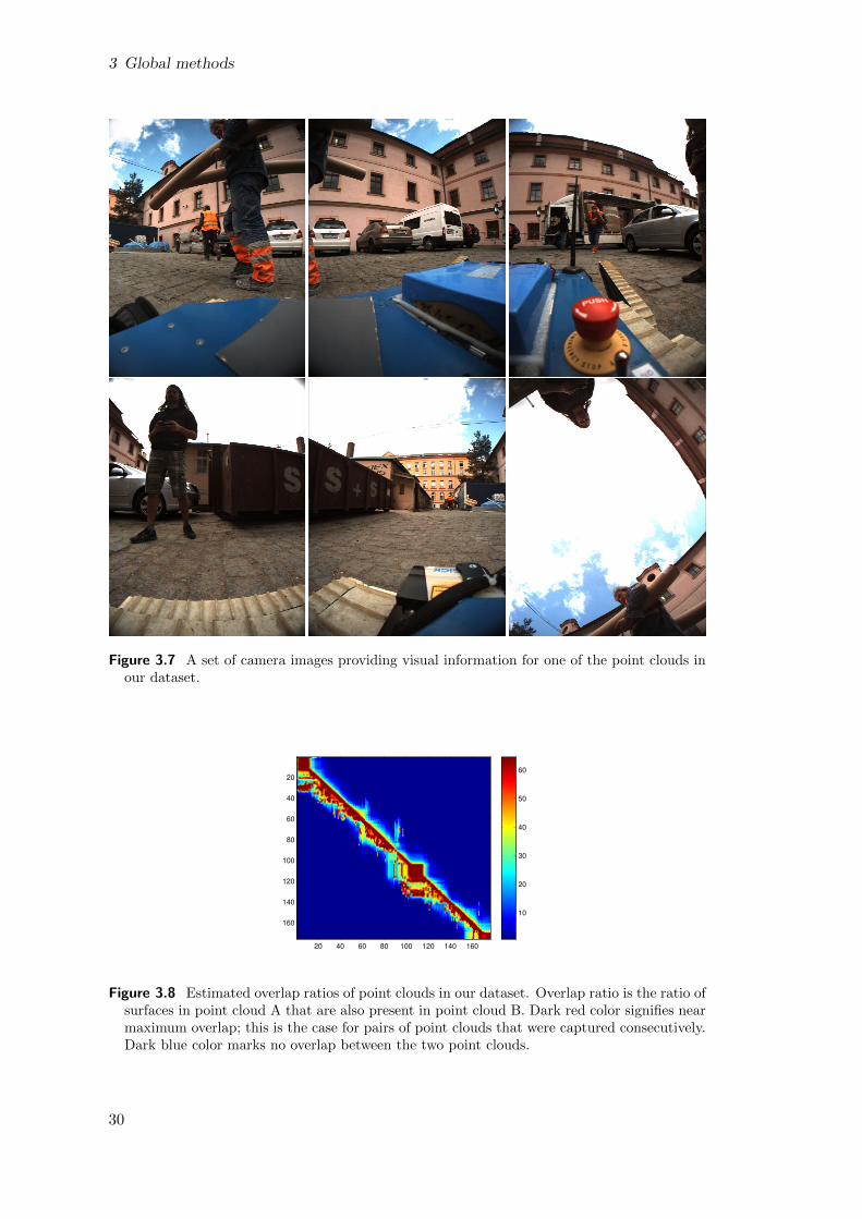
We have extracted a series of 176 point clouds along with the corresponding cameraimages from a recording of a courtyard at the CTU campus at Charles Square. Duringthe scanning process, the robot moves in an outdoor, building-surrounded environment.To select point cloud pairs, we followed the procedure described in [21]: for each pairof the clouds, we have estimated the overlap ratio (see figure 3.8), and based on thatinformation we have selected 35 pairs of scans, with overlap ratios distributed uniformlybetween 30 % and 99 %.
We do not consider any perturbations of the initial pose in this dataset. There aretwo reasons to do so: firstly, global registration methods provide similar results forarbitrary initial poses, therefore perturbations are unnecessary to test these methods.Secondly, our cameras are calibrated so that only the point clouds in the undistortedinitial pose are projected correctly into the camera images.
3.5 Experimental results
Although our dataset is small and its ground truth is relatively imprecise, it is suffi-cient for our purposes. We compare the original, unaltered method by Petricek andSvoboda[19] to the method that contains one of the proposed changes. At the sametime, we take the opportunity to test various parameter configurations of our version
29
3 Global methods
Figure 3.7 A set of camera images providing visual information for one of the point clouds inour dataset.
20 40 60 80 100 120 140 160
20
40
60
80
100
120
140
160
10
20
30
40
50
60
Figure 3.8 Estimated overlap ratios of point clouds in our dataset. Overlap ratio is the ratio ofsurfaces in point cloud A that are also present in point cloud B. Dark red color signifies nearmaximum overlap; this is the case for pairs of point clouds that were captured consecutively.Dark blue color marks no overlap between the two point clouds.
30
3.5 Experimental resultsSheet2
Page 1
0
5
10
15
20
25
30
Descriptor: Correct correspondences (%)
originals = 1/4 ms = 1/2 ms = 1 ms = 2 ms = 4 m
0
5
10
15
20
25
30
RFD: Correct correspondences (%)
originalσ = 1/4 mσ = 1/2 mσ = 1 mσ = 2 mσ = 4 m
0
5
10
15
20
25
30
Correct correspondences (%)
originalRFDdescriptordescriptor & RFD
0
5000
10000
15000
20000
25000
30000
Descriptor: number of correspondences
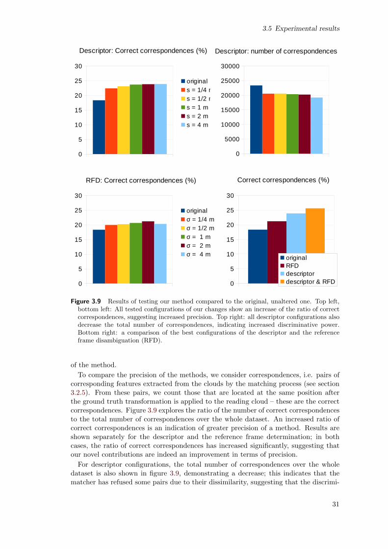
Figure 3.9 Results of testing our method compared to the original, unaltered one. Top left,bottom left: All tested configurations of our changes show an increase of the ratio of correctcorrespondences, suggesting increased precision. Top right: all descriptor configurations alsodecrease the total number of correspondences, indicating increased discriminative power.Bottom right: a comparison of the best configurations of the descriptor and the referenceframe disambiguation (RFD).
of the method.
To compare the precision of the methods, we consider correspondences, i.e. pairs ofcorresponding features extracted from the clouds by the matching process (see section3.2.5). From these pairs, we count those that are located at the same position afterthe ground truth transformation is applied to the reading cloud – these are the correctcorrespondences. Figure 3.9 explores the ratio of the number of correct correspondencesto the total number of correspondences over the whole dataset. An increased ratio ofcorrect correspondences is an indication of greater precision of a method. Results areshown separately for the descriptor and the reference frame determination; in bothcases, the ratio of correct correspondences has increased significantly, suggesting thatour novel contributions are indeed an improvement in terms of precision.
For descriptor configurations, the total number of correspondences over the wholedataset is also shown in figure 3.9, demonstrating a decrease; this indicates that thematcher has refused some pairs due to their dissimilarity, suggesting that the discrimi-
31
3 Global methods
0 0.1 0.2 0.3 0.4 0.5 0.6 0.70
0.05
0.1
0.15
0.2
0.25
0.3
0.35
0.4
0.45
Cumulative probability
Ro
tatio
na
l d
isp
lace
me
nt
[ra
d]
patch size 1/4 m
patch size 1/2 m
patch size 1 m
patch size 2 m
patch size 4 m
original method
0.65 0.7 0.75 0.8 0.85 0.9 0.95 10
0.5
1
1.5
2
2.5
3
3.5
Cumulative probability
Ro
tatio
na
l d
isp
lace
me
nt
[ra
d]
patch size 1/4 m
patch size 1/2 m
patch size 1 m
patch size 2 m
patch size 4 m
original method
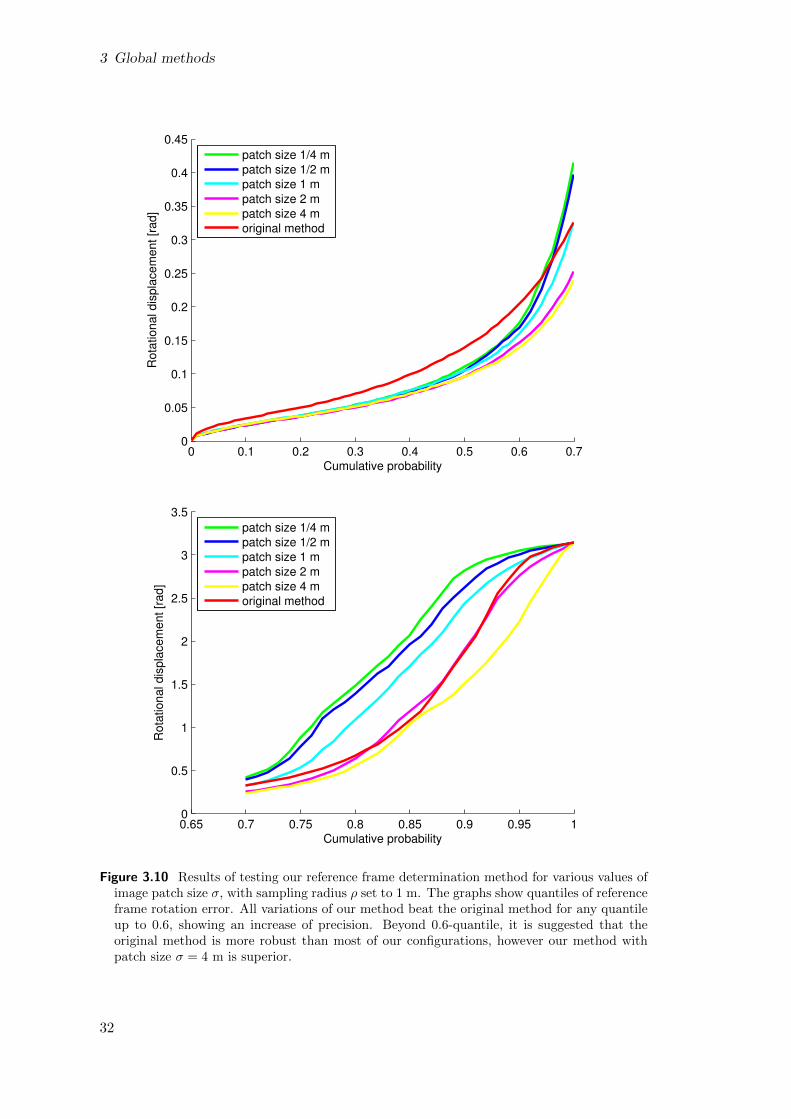
Figure 3.10 Results of testing our reference frame determination method for various values ofimage patch size σ, with sampling radius ρ set to 1 m. The graphs show quantiles of referenceframe rotation error. All variations of our method beat the original method for any quantileup to 0.6, showing an increase of precision. Beyond 0.6-quantile, it is suggested that theoriginal method is more robust than most of our configurations, however our method withpatch size σ = 4 m is superior.
32
3.6 Conclusion
native power of the descriptor has increased.Additionally, regarding reference frame determination, we consider rotation displace-
ment of the reference frames. First, we identify the keypoints that have the same po-sition in the clouds after being aligned using ground truth. For each pair, we computethe displacement of the reference frames using equation (2.5). We gather the rotationerror of reference frames over the whole dataset, and analyze it using quantiles.
Figure 3.10 shows the quantiles of the rotation error. Our method excels in the0 to 0.6-quantile range, suggesting its precision is an improvement over the originalmethod in most cases. Over the 0.6-quantile, the original method beats most of ourconfigurations, showing that it is quite robust. However, one of our configurations(σ = 4 m) overcomes all other tested methods for any quantile.
3.6 Conclusion
We have proposed, implemented and tested two independent enhancements to themethod by Petricek and Svoboda[19]: a new descriptor, and a new method of ref-erence frame determination. Both of our contributions are a success, showing signifi-cantly improved capabilities over the original, unaltered method. We have achieved thegoal of improving the original method based on the availability of visual information,in particular camera imagery.
We have successfully applied solutions from image registration methods, specificallySURF[8], to point cloud registration. As the challenging datasets by Pomerleau etal.[22] lack visual information, we have created our own dataset, based on range andvisual data captured in an outdoor environment. The result of our work is a competitiveglobal registration method. With that said, we do not believe that the possibilities ofcolor-aware point cloud registration are exhausted. On the contrary, the subject matteris still largely unexplored, creating room for future work.
33
4 Conclusions
In our work, we focused on point cloud registration methods. A different approach wasemployed for each of the two classes of methods, local and global; local registrationmethods were approached investigatively, offering an insightful view into their capabili-ties. For the global methods however, a more generative approach was applied, creatinga method that takes advantage of visual data.
For the purposes of local method comparison, experiments were carried out thatmake use of an existing, publicly available protocol, based on a number of high-qualitydatasets. To inspect the capabilities of the methods in a greater detail, an additionalprotocol based on the same datasets was created; by evaluating our protocol, it ispossible to study the capabilities of the methods in an unprecedented detail, overcomingany previous work that we know of. Limitations of the examined methods are revealed inthe form of maximum viable initial pose displacement, provided that error requirementsare given. Additionally, results for methods that were neglected in our experiments canbe received at a later date and directly compared to ours.
Analyzing the results, it is shown that of the tested methods, the iterative clos-est point (ICP) algorithm configured by Kubelka et al.[15], and the three-dimensionalnormal distribution transform (3D-NDT) algorithm implemented in the Point CloudLibrary[5] share the lead in registration quality. Using these methods for point cloudregistration is recommended. Two composite methods were created and tested, butwere not proven useful.
Concerning global methods, a feature-based method by Petricek and Svoboda[19] wasenhanced using visual information from cameras. Two changes have been proposed, anextension of the descriptor, and a modification of reference frame determination. Partsof the SURF[8] algorithm have been used to extract visual information, introducing animage registration technique into point cloud registration. A dataset containing visualdata was created to test our proposals, along with a testing protocol.
Using the protocol, the original method was evaluated, as well as its modifications.The modifications are shown to be effective, overcoming the unaltered version of themethod; extended descriptor increases the number of correct feature correspondences,and changes in reference frame determination decrease the rotation error of the estab-lished reference frames. The goal of improving a feature-based registration method byfusing visual and range data was accomplished.
We believe that the subject of visual data-enhanced point cloud registration is notyet fully explored. Our suggestions of future work include: exploring the use of coloredpoint clouds, as opposed to camera imagery; investigating three-dimensional binarydescriptors, e.g. a modification of BRAND[18], in the context of visual data; usingvisual data to improve the saliency measure for keypoint detection; and extending ourmethod to make use of color information other than intensity.
34
Bibliography
[1] Adaptive traversability. http://cw.felk.cvut.cz/wiki/misc/projects/nifti/sw/adaptive_traversability. Accessed on May 23, 2014. 3
[2] The best known packings of equal circles in a circle. http://hydra.nat.
uni-magdeburg.de/packing/cci/cci.html. Accessed on May 23, 2014. 28
[3] Camera calibration and 3D reconstruction. http://docs.opencv.org/modules/
[5] PCL - point cloud library. http://pointclouds.org/. Accessed on May 23, 2014.10, 34
[6] Summed area table. http://en.wikipedia.org/wiki/Summed_area_table. Ac-cessed on May 23, 2014. 25
[7] Michel A. Audette, Frank P. Ferrie, and Terry M. Peters. An algorithmic overviewof surface registration techniques for medical imaging. Medical Image Analysis,4(3):201 – 217, 2000. 2
[8] Herbert Bay, Andreas Ess, Tinne Tuytelaars, and Luc Van Gool. Speeded-uprobust features (SURF). Comput. Vis. Image Underst., 110(3):346–359, June 2008.22, 25, 26, 27, 28, 33, 34
[9] P.J. Besl and Neil D. McKay. A method for registration of 3-D shapes. Pat-tern Analysis and Machine Intelligence, IEEE Transactions on, 14(2):239–256,Feb 1992. 4, 10
[10] P. Biber and W. Straßer. The normal distributions transform: a new approachto laser scan matching. In Intelligent Robots and Systems, 2003. (IROS 2003).Proceedings. 2003 IEEE/RSJ International Conference on, volume 3, pages 2743–2748 vol.3, Oct 2003. 4, 6
[11] Y. Chen and G. Medioni. Object modeling by registration of multiple range im-ages. In Robotics and Automation, 1991. Proceedings., 1991 IEEE InternationalConference on, pages 2724–2729 vol.3, Apr 1991. 4, 10
[12] Jan Elseberg, Stephane Magnenat Rol, and Siegwart Andreas Nuchter. Compar-ison of nearest-neighbor-search strategies and implementations for efficient shaperegistration, 2012. 4
[13] B. Huhle, Martin Magnusson, W. Strasser, and A.J. Lilienthal. Registration ofcolored 3D point clouds with a kernel-based extension to the normal distributionstransform. In Robotics and Automation, 2008. ICRA 2008. IEEE InternationalConference on, pages 4025–4030, May 2008. 6
[14] A.E. Johnson and M. Hebert. Using spin images for efficient object recognition incluttered 3D scenes. Pattern Analysis and Machine Intelligence, IEEE Transac-tions on, 21(5):433–449, May 1999. 21, 22, 23
[15] Vladimır Kubelka, Lorenz Oswald, Francois Pomerleau, Francis Colas, Tomas Svo-boda, and Michal Reinstein. Robust data fusion of multi-modal sensory informa-tion for mobile robots. Journal of Field Robotics, in press. 4, 5, 9, 10, 20, 29,34
[16] David G. Lowe. Distinctive image features from scale-invariant keypoints. Int. J.Comput. Vision, 60(2):91–110, November 2004. 22
[17] Martin Magnusson. The Three-Dimensional Normal-Distributions Transform —an Efficient Representation for Registration, Surface Analysis, and Loop Detection.PhD thesis, Orebro University, December 2009. Orebro Studies in Technology 36.4
[18] E.R. Nascimento, G.L. Oliveira, M. F M Campos, A.W. Vieira, and W.R. Schwartz.BRAND: A robust appearance and depth descriptor for RGB-D images. In Intel-ligent Robots and Systems (IROS), 2012 IEEE/RSJ International Conference on,pages 1720–1726, Oct 2012. 22, 23, 24, 34
[19] T. Petricek and T. Svoboda. Point cloud registration from local feature correspon-dences - evaluation on challenging datasets. Unpublished work, under review. 22,23, 24, 25, 26, 27, 29, 33, 34
[20] T. Petricek and T. Svoboda. Area-weighted surface normals for 3D object recog-nition. In ICPR’12, pages 1492–1496, 2012. 22, 23
[21] Francois Pomerleau, Francis Colas, Roland Siegwart, and Stephane Magnenat.Comparing ICP variants on real-world data sets. Autonomous Robots, 34(3):133–148, 2013. 4, 5, 8, 10, 29
[22] Francois Pomerleau, Ming Liu, Francis Colas, and Roland Siegwart. Challengingdata sets for point cloud registration algorithms. The International Journal ofRobotics Research, 31(14):1705–1711, 2012. 7, 8, 29, 33
[23] R.B. Rusu, N. Blodow, and M. Beetz. Fast point feature histograms (FPFH) for3D registration. In Robotics and Automation, 2009. ICRA ’09. IEEE InternationalConference on, pages 3212–3217, May 2009. 21, 22, 23
[24] T. Stoyanov, Martin Magnusson, and A.J. Lilienthal. Point set registration throughminimization of the L2 distance between 3D-NDT models. In Robotics and Au-tomation (ICRA), 2012 IEEE International Conference on, pages 5196–5201, May2012. 6
[25] F. Tombari, S. Salti, and L. Di Stefano. Unique signatures of histograms for localsurface description. In 11th European Conference on Computer Vision (ECCV10), pages 356–369, Hersonissos, Crete, Greece, September 2010. 21, 22, 23