Center for Biofilm Engineering Marty Hamilton Professor Emeritus of Statistics Montana State University Statistical design & analysis for assessing the efficacy of instructional modules CS 580 April 24, 2006
Transcript
Center for Biofilm Engineering
Marty HamiltonProfessor Emeritus of StatisticsMontana State University
Statistical design & analysis for assessing the efficacy of
instructional modules
CS 580 April 24, 2006
Why Statistics?
Provide convincing results
Improve communication
“...I do not mean to suggest that computers eliminate stupidity---they may in fact encourage it.”Robert P. Abelson, in Statistics as Principled Argument(cited on Rocky Ross’s CS 580 home page)
What is Statistics?
Data
Design
Uncertainty assessment
Statistical Thinking
Data
Design
Uncertainty assessment
Data: Choosing thequantity to measure
Reliable test of knowledge
Quantitative response
Statistical thinking
Data
Design
Uncertainty assessment
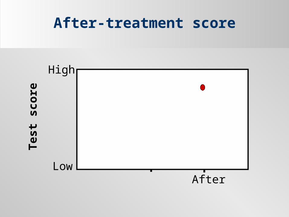
After-treatment score
A student used the modules, then scored 80% on the test
Conclusion: modules have high efficacy
Data: Choosing thequantity to measure
Reliable tests of knowledge:before-treatment testafter-treatment test
Quantitative response: difference in test scores, after-treatment minus before-treatment
After-treatment score
High
Low
Test
score
After
Before- and after-treatment scores
High
LowAfterBefore
Test
score
Response
Difference between before- and after-treatment scores
A student used the modules, then scored 50 points higher on the after-treatment test than on the before treatment test (Response = 50).
Conclusion: modules have high efficacy
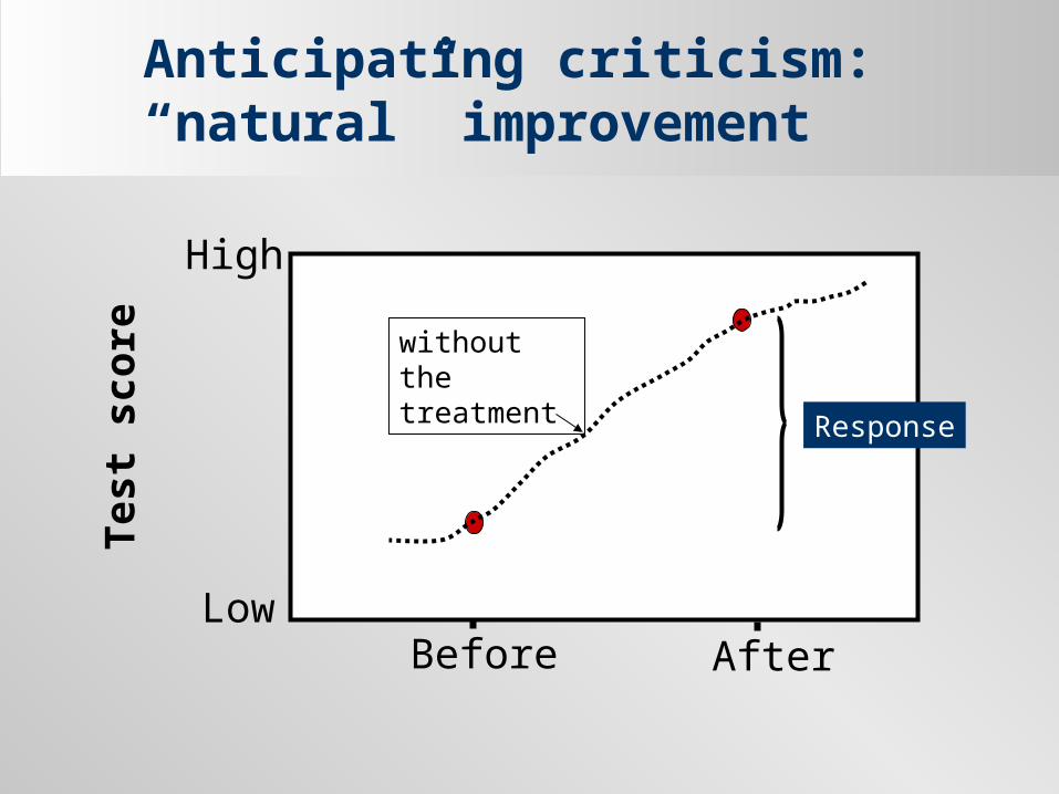
Anticipating criticism: “natural” improvement
High
LowAfterBefore
Test
score without the
treatment
Response
Anticipating criticism
Before/after observations for just the “treated” student may not accurately represent the treatment effect
May need treated and untreated students (i.e., a control)
Control or comparison
The control can be either a negative control or positive control
A student taking a conventional classroom lecture/recitation course would provide a positive control or comparison
(placebo)(best conventional)
Difference scores for each of 12 students, 6 per group
100
0Treatedgroup
Controlgroup
D
iffere
nce
(aft
er
– b
efo
re)
Of practical importance?
Study design
Before and after test scores for each student in both the treated and control groups
.Minitab: FirstStudy_CS580.MTWShow data layout ... matrix
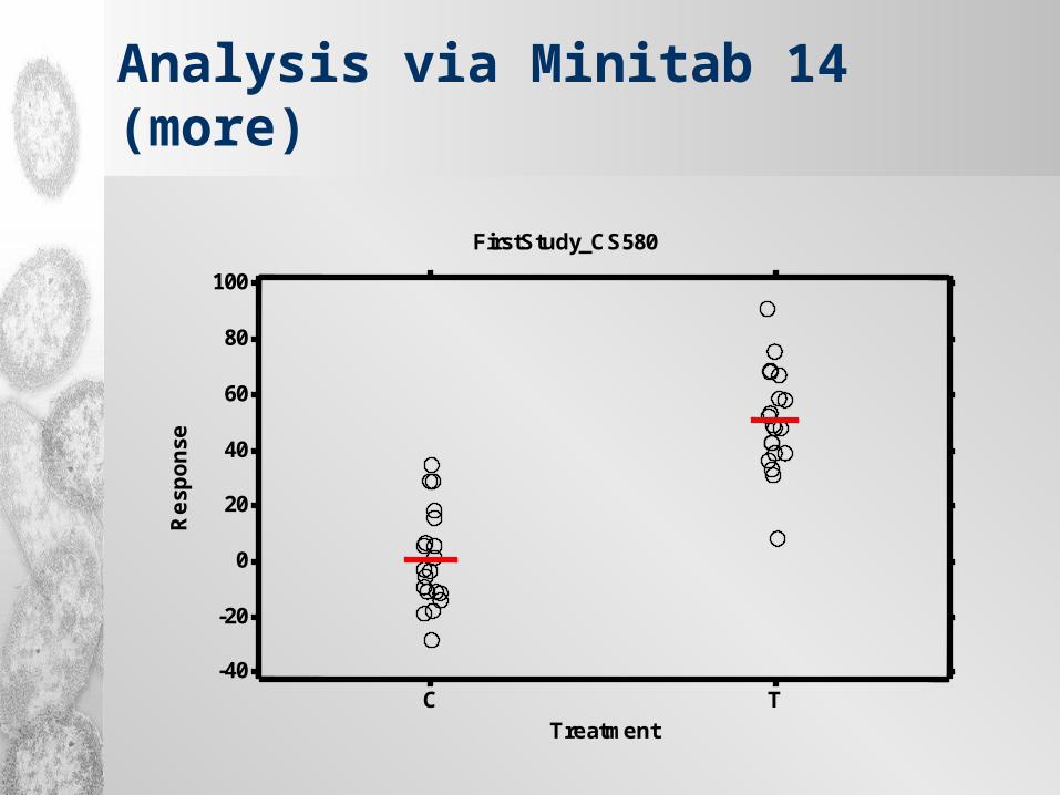
Stat > Basic Statistics > Display Descriptive Statistics ... Ask for individual value plotStat > Basic Statistics > 2 Sample t ...Minitab outputTwo-Sample T-Test and CI: Response, Treatment Two-sample T for ResponseTreatment N Mean StDev SE MeanC 20 0.6 17.4 3.9T 20 50.6 18.4 4.1Difference = mu (C) - mu (T)Estimate for difference: -50.016495% CI for difference: (-61.4656, -38.5672)T-Test of difference = 0 (vs not =): T-Value = -8.84 P-Value = 0.000 DF = 38Both use Pooled StDev = 17.8846
Null hypothesis: true mean response for Treatment = true mean response for Control Conclusions:
1. Reject the null hypothesis because it is discredited by the data (p-value < 0.001)2. 95% confident that the treatment mean response is between 38.6 and 61.5 larger than
the true control mean response3. Is this efficacy repeatable?
Analysis via Minitab 14 (more)
Treatment
Re
spo
nse
TC
100
80
60
40
20
0
-20
-40
FirstStudy_CS580
Analysis via Minitab 14 (more)
Minitab: SixStudies_CS580.MTWShow data layout ... matrix
Stat > Tables > Descriptive Statistics Minitab outputTabulated statistics: Replicate, Treatment Rows: Replicate Columns: Treatment C T All
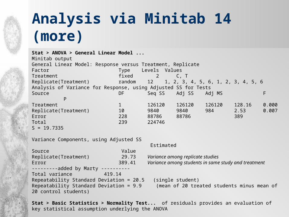
Stat > ANOVA > General Linear Model ...Minitab outputGeneral Linear Model: Response versus Treatment, Replicate Factor Type Levels ValuesTreatment fixed 2 C, TReplicate(Treatment) random 12 1, 2, 3, 4, 5, 6, 1, 2, 3, 4, 5, 6Analysis of Variance for Response, using Adjusted SS for TestsSource DF Seq SS Adj SS Adj MS F PTreatment 1 126120 126120 126120 128.16 0.000Replicate(Treatment) 10 9840 9840 984 2.53 0.007Error 228 88786 88786 389Total 239 224746S = 19.7335
Variance Components, using Adjusted SS EstimatedSource ValueReplicate(Treatment) 29.73 Variance among replicate studiesError 389.41 Variance among students in same study and treatment---------added by Marty ----------Total variance 419.14 Repeatability Standard Deviation = 20.5 (single student)Repeatability Standard Deviation = 9.9 (mean of 20 treated students minus mean of 20 control students)
Stat > Basic Statistics > Normality Test... of residuals provides an evaluation of key statistical assumption underlying the ANOVA
Analysis via Minitab 14 (more)
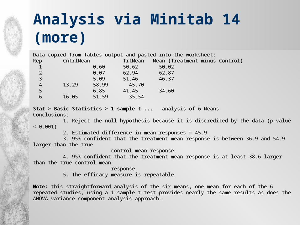
Data copied from Tables output and pasted into the worksheet: Rep CntrlMean TrtMean Mean (Treatment minus Control) 1 0.60 50.62 50.02 2 0.07 62.94 62.87 3 5.09 51.46 46.37 4 13.29 58.99 45.70 5 6.85 41.45 34.60 6 16.05 51.59 35.54
Stat > Basic Statistics > 1 sample t ... analysis of 6 MeansConclusions:
1. Reject the null hypothesis because it is discredited by the data (p-value < 0.001)2. Estimated difference in mean responses = 45.93. 95% confident that the treatment mean response is between 36.9 and 54.9 larger than the true
control mean response4. 95% confident that the treatment mean response is at least 38.6 larger than the true control mean
response5. The efficacy measure is repeatable
Note: this straightforward analysis of the six means, one mean for each of the 6 repeated studies, using a 1-sample t-test provides nearly the same results as does the ANOVA variance component analysis approach.
Trade-offs: What is themain source of variability?
It is often more important to repeat the study
than to expend time and materialsfinding a precise efficacy estimate for a single study.