Working Paper No. 193 Central Bank Purchases of Government Bonds Samuel Huber and Jaehong Kim April 2015 University of Zurich Department of Economics Working Paper Series ISSN 1664-7041 (print) ISSN 1664-705X (online)
Transcript
Working Paper No. 193
Central Bank Purchases of Government Bonds
Samuel Huber and Jaehong Kim
April 2015
University of Zurich
Department of Economics
Working Paper Series
ISSN 1664-7041 (print) ISSN 1664-705X (online)
Central Bank Purchases of Government Bonds
Samuel HuberUniversity of Basel
Jaehong KimChapman University
April 29, 2015
Abstract
We develop a microfounded model, where agents have the possibility to trade moneyfor government bonds in an over-the-counter market. It allows us to address important openquestions about the e¤ects of central bank purchases of government bonds, these being: underwhat conditions these purchases can be welfare-improving, what incentive problems theymitigate, and how large these e¤ects are. Our main �nding is that this policy measure canbe welfare-improving, by correcting a pecuniary externality. Concretely, the value of moneyis increased as central bank�s purchases of government bonds induce agents to increase theirdemand for money, which is welfare-improving.
Quantitativ Easing (QE, hereafter) denotes a central bank policy of purchasing �nancial assetssuch as government bonds, agency debt, or mortgage-backed securities. Empirical evidence sug-gests that QE is successful in reducing yields on these assets, while there is no sound conclusionabout its e¤ects on the allocation and welfare.1
In this paper, we focus on the e¤ects of central bank purchases of government bonds. Forthis purpose, we construct a microfounded monetary model, where trading in �nancial marketsis essential. The model allows us to understand which incentive problems QE mitigates, how to�nd the optimal degree of QE, under what conditions it is successful and what e¤ects it has onquantities and prices.
In our model, agents face idiosyncratic liquidity shocks, and they hold a portfolio composed ofmoney and government bonds. Money can be directly used to purchase goods and thus serves as
1See, for instance, Gagnon et al. (2011), D�Amigo and King (2012), Krishnamurthy and Vissing-Jorgensen(2012), or Bauer and Neely (2013), among others.
1
a medium of exchange. In contrast, government bonds cannot be used as a medium of exchange,but are a superior store of value.2 The idiosyncratic liquidity shocks generate an ex-post ine¢ cientallocation of the medium of exchange: Some agents will hold money, but have no current needfor it, while other agents will hold insu¢ cient amounts of money in order to satisfy their liquidityneeds. A secondary �nancial market allows agents to trade money for bonds and so improvesthe allocation of the medium of exchange. The secondary �nancial market is an over-the-countermarket, that embeds the recent advances in search theory.3 QE is modelled as a central bankpurchase of government bonds funded by the issuance of money; i.e., we abstract from the issuanceof interest-bearing reserves and assume that the central bank directly controls the bond-to-moneyratio. There are no aggregate shocks, and we derive our results in the monetary steady stateequilibrium. Furthermore, we focus on the optimal degree of QE in an economy, where thee¢ cient allocation is not attainable; i.e., on an economy with in�ation rates above the Friedmanrule.
Our main �nding is that QE mitigates a pecuniary externality and so improves the allocationand welfare. This externality arises because in our incomplete market model the resulting equi-libria might not be constrained e¢ cient. In such an environment, government interventions canbe welfare-improving.4 In our model, the secondary �nancial market reduces the incentive to self-insure against liquidity shocks, and agents attempt to bene�t from money held by other marketparticipants. As a result, the aggregate demand for money is too low, and QE can mitigate thisexternality. The reasoning behind this result is as follows. QE reduces the bond-to-money ratioand as a result bonds become scarce and are priced above their fundamental value. This inducesagents to increase their demand for money, which marginally increases the value of money and sothe insurance for all market participants. This �nding is very novel and not present in previousstudies about the e¤ects of QE. A further contribution of our work is that we show that QE isonly successful for low in�ation rates.
We calibrate the model to U.S. data in order to estimate the impact of QE on quantities andprices. For our baseline calibration, we �nd that the optimal degree of QE succeeds in reducingthe yield of bonds by 0:52 percent. The social bene�ts associated with such a policy measureaccount for 0:014 percent of steady state consumption. Furthermore, we �nd that QE is onlywelfare-improving for in�ation rates below 8 percent. The higher the bargaining power of bondvendors, the higher the bene�ts of QE and the higher the critical in�ation rate up to which thispolicy measure is welfare-improving. In contrast, the lower the search frictions, the lower thebene�ts and the lower the critical in�ation rate up to which QE is bene�cial.
Based on empirical evidence, we argue that for the U.S. a calibration with equally distributedbargaining power among agents and low search frictions seems more realistic than our baseline
2 It is socially bene�cial that government bonds cannot be used as a medium of exchange. Otherwise, bondswould be perfect substitutes for money and thus be redundant. See Kocherlakota (2003), Andolfatto (2011),Berentsen and Waller (2011), or Berentsen et al. (2014), for a more detailed discussion.
3There is a rapidly growing literature which builds on the seminal contribution of Du¢ e et al. (2005). See, forinstance, Du¢ e et al. (2008), Lagos and Rocheteau (2009), Lagos, Rocheteau and Weill (2011), Rocheteau andWright (2013), Geromichalos and Herrenbrueck (2014), Geromichalos et al. (2014), or Berentsen et al. (2015b).
4See, for instance, Greenwald and Stiglitz (1986) or Berentsen et al. (2015b) for a more detailed discussion.
2
calibration. In such a case, the bene�ts associated with a central bank policy of purchasing gov-ernment bonds are likely to be small and in the area of 0:002 percent of steady state consumption.Furthermore, such a policy measure is only bene�cial for in�ation rates below 4:3 percent andreduces the yield of bonds by 0:40 percent. Hence, even though we can verify that QE provescompetent in substantially reducing the yield of bonds, our �ndings indicate that the overallsocial bene�ts are likely to be anemic.
In our model, an equilibrium can be of three types, which we denote by type-I, type-II, andtype-III. In a type-I and a type-II equilibrium, bonds are priced at their fundamental value, andQE does not e¤ect welfare. The reason is that trading is unconstrained in the type-I equilibrium,while in the type-II equilibrium only the cash constraint on bond buyers is binding. In contrast,in a type-III equilibrium, bonds are priced above their fundamental value and exhibit a liquiditypremium. The reason is that in this equilibrium the bond constraint on bond vendors is binding.Therefore, in a type-III equilibrium QE has a direct impact on the allocation and welfare. Asummary of the bond prices and the trading constraints in the respective equilibria is shown inTable 1:
Table 1: Bond prices and trading constraints
Equilibrium Bond Price Bond Constraint Cash ConstraintType-I Fundamental Non-Binding Non-BindingType-II Fundamental Non-Binding BindingType-III Liquidity Premium Binding Non-Binding
In Figure 1, we show the regions of existence with respect to the in�ation rate and the bond-to-money ratio B. Furthermore, the �gure also shows the optimal choice of B, which coincideswith the optimal degree of QE.
Figure 1: Regions of existence and optimal B
3
The Friedman-rule is shown at the bottom-left corner of the above �gure, where the in�ationrate equals the rate of time preference, �. At the Friedman-rule, �nancial intermediation isredundant, and the e¢ cient allocation is attainable. For in�ation rates � < < 12, eitherthe type-I or the type-III equilibrium exists. Hereafter, we will show that it is always welfare-improving to reduce the bond-to-money ratio in the type-I equilibrium, such that the bondconstraint becomes binding, and the economy moves to a region in the type-III equilibrium,where welfare is maximized (highlighted by the green line).5 For in�ation rates above 12, eitherthe type-II or the type-III equilibrium exists. The triangle in the top-right section shows thatthere may exist a region, where the type-II and the type-III equilibrium coexist. We show, thatfor > 12 and su¢ ciently close to 12, welfare is also maximized in the type-III equilibrium;i.e., QE is welfare-improving. However, if > 12 and is considerably higher than 12, thenwelfare is maximized in the type-II equilibrium, and the optimal policy is to keep the bond-to-money ratio at least at the border to the type-II equilibrium. In other words, if in�ation is toohigh, a central bank policy of purchasing government bonds does not improve welfare, but ismore likely to reduce it.
2 Literature
Williamson (2012) analyses the e¤ects of central bank purchases of government bonds in a modelbuilding on Lagos and Wright (2005). In the baseline model, he assumes that in non-monitoredmeetings producers only accept money in exchange for goods, while in monitored-meetings theyalso accept claims to government bonds. As banks operate after consumers learn in which typeof meeting they will participate in the subsequent goods market, consumers in the �rst type ofmeeting withdraw cash from the bank, while consumers in the second type of meeting receive theright to trade claims to bonds. When a consumer meets a producer in a monitored meeting, thenhe makes a take-it-or-leave it o¤er; i.e., he has all the bargaining power in the match. Williamson�nds that a central bank purchase of government bonds only has an e¤ect on quantities and pricesin an equilibrium where bonds are scarce. That is, in such an equilibrium this policy measurefurther reduces the supply of bonds and thus results in an increase of the liquidity premium onbonds; i.e., in a decrease of the real interest rate. As a result, it reduces the availability of claimsto bonds in monitored meetings. The author then extends the model to include privately issueddebt beside government debt. In the extended version, he �nds that due to the reduction in thestock of government bonds, a central bank purchase of government bonds induces an expansionof private debt; i.e., a higher issuance of corporate bonds. Thereafter, he includes additional�nancial market frictions in order to analyse issues in �nancial crises. He argues that if anexogenous shock results in a complete shut-down of the credit market, such that the economyends up in an equilibrium where bonds are scarce, then a central bank purchase of governmentbonds may result in a further reduction in the real interest rate and worsen the scarcity problem,rather than improve it.
5Note that we assume that �scal policy is passive and that, therefore, any change in the bond-to-money ratioB has no e¤ect on the in�ation rate . This will be clari�ed in Section 5.
4
Williamson (2014a) constructs a model of money, credit and banking, where he analyzescentral bank purchases of long-maturity government bonds, denoted as QE.6 Like in Williamson(2012), trade in the goods market is performed by money and claims to bonds. Williamson(2014a) focuses his analysis on an equilibrium where government bonds are scarce and thusare priced above their fundamental value. He �nds that a scarcity of government bonds, aswell as inferior properties of long-maturity bonds when used as collateral compared to short-maturity bonds, are preconditions for the existence of a term premium. Furthermore, he �ndsthat QE reduces the yield of long-maturity bonds, which results in a �attening of the yield curve.Additionally, QE reduces in�ation and so increases the real yield of bonds, even though thenominal yield falls. This increases the value of collateralizable wealth and so relaxes the bank�scollateral constraints, which is welfare-improving. Note, that the above result is derived for acentral bank applying a �oor system, while a channel system limits the central banks�ability toperform QE.
Williamson (2014b) builds on Williamson (2012 and 2014a) and analyses the e¤ects of centralbank purchases of private assets in an economy where agents have incentives to fake the qualityof collateral. Consumers own houses which are used as collateral to obtain a mortgage. Like inWilliamson (2012 and 2014a), trade in the goods market is performed by money and claims to�nancial assets; i.e., claims to mortgages, government debt, and reserves. Consumers (banks) havethe ability to fake the quality of houses (mortgages) at a cost. Also Williamson (2014b) focuseshis analysis on an equilibrium where �nancial assets are scarce, and thus government bonds arepriced above their fundamental value. If the cost of faking is low, then mortgages exhibit aninterest rate spread and haircuts to convince lenders that the collateral is not faked. In suchan environment, a central bank purchase of mortgages might not be feasible as the central bankmight not be able to verify the quality of the private assets. Hence, only when the cost of fakingis su¢ ciently high, such that neither consumers nor banks have an incentive to fake the qualityof the collateral before the program starts, it might then be welfare-improving for a central bankto purchase private assets from banks. He �nds that in order to be successful, the central bankneeds to purchase the entire amount of outstanding mortgages. Doing so and issuing governmentbonds at same time, relaxes the bank�s collateral constraints, which is welfare-improving.
Gertler and Karadi (2013) develop a macroeconomic model to analyze the e¤ects of centralbank purchases of long-maturity government bonds or private loans, denoted as large-scale assetpurchases. Their model has some similarities to Williamson (2012, 2014a, and 2014b); i.e.,they also assume that banks need to collateralize their deposits and that bonds with di¤erentmaturities and from di¤erent issuers (government or private) have di¤erent properties for beingused as collateral. However, Gertler and Karadi (2013) do not model the intermediation of banksexplicitly, but rather assume that households can only hold short-term government bonds andbank deposits, which are in turn collateralized by private debt and long-term government bonds.They argue that central banks, as opposed to private intermediaries, obtain funds elastically;i.e., they can fund the purchase of long-term securities by issuing short-term debt. This provides
6The basic framework builds on Lagos and Wright (2005) and Rocheteau and Wright (2005), and has a similarstructure to that of Williamson (2012).
5
central banks with a channel for large-scale asset purchases to be e¤ective in reducing borrowingcosts, if the aggregate balance sheet constraint of banks is binding; i.e., if �nancial assets arescarce. They �nd, further, that large-scale asset purchases help to �atten the yield curve, whichworks especially well when short-term rates are not expected to rise anytime soon.
Herrenbrueck (2014) develops a model where agents can trade �nancial assets (governmentbonds and physical capital) in over-the-counter markets in the spirit of Du¢ e et al. (2005). Theover-the-counter markets feature search frictions in the way that agents need to �nd a broker totrade with. Once matched, agents make a take-it-or-leave-it o¤er to the broker; i.e., they have allthe bargaining power in the match. The author �nds that QE, de�ned as a central bank purchaseof government bonds, results in an increase in the price of �nancial assets and so transfers wealthto agents who value it more; i.e., to agents who want to sell �nancial assets for money in order toconsume. In turn, this reallocation of purchasing power stimulates consumption and investment.The drawback of this policy measure is that it reduces the available stock of bonds and that itdepresses the private �ow of funds, which results in a less e¢ cient allocation of money. WhetherQE is bene�cial depends on which of the e¤ects dominates.
In contrast to the above studies, we abstract from private assets, the central bank issuanceof interest-bearing reserves, or brokers, and clearly focus on the economic mechanisms behindcentral bank purchases of government bonds funded by the issuance of money. Furthermore,we explicitly model bargaining frictions in the secondary bond market, which we believe arenecessary ingredients for any over-the-counter market. We �nd that the main welfare-improvingaspect of QE is that it corrects a pecuniary externality, and not that it transfers wealth to agentswho value it more. In other words, it is not the resulting liquidity premium on bonds thatimproves welfare, but the incentive to increase the demand for money. Besides this, we show thefull picture and do not solely focus on an equilibrium where bonds are scarce. This allows us tostate up to which in�ation rate QE is successful, thus providing an argument which is missing inthe above studies.
Our paper is therefore also related to the literature that focuses on correcting pecuniaryexternalities, such as Berentsen et al. (2014 and 2015b). Berentsen et al. (2014) �nd that addingsearch frictions to a competitive secondary �nancial market can be welfare-improving for highin�ation rates. The reason is that adding search frictions increases the demand for money, whichis welfare-improving, but it also increases consumption variability, since only some agents haveaccess to the secondary �nancial market. In a similar framework to ours, Berentsen et al. (2015b)�nd that the demand for money is too low in an equilibrium where trading is unconstrained andthat imposing a �nancial transaction tax can correct this externality. However, imposing a�nancial transaction tax requires the central bank to operate the secondary �nancial market inorder to perfectly enforce tax payment. In contrast, QE only requires the central bank to issuemoney in order to purchase government bonds, which is much easier to implement. In view ofits tactical simplicity, QE has recently experienced much more popularity among policy makersthan implementing a �nancial transaction tax. Thus, it is crucial to understand the economicmechanisms behind such a policy measure.
6
3 Environment
A [0; 1]-continuum of agents live forever in discrete time. In each period, there are three marketsthat open sequentially.7 The �rst market is a secondary bond market, where agents trade moneyfor nominal bonds. The second market is a goods market, where agents produce or consumemarket-2 goods. The third market is a centralized market, where all agents consume and producemarket-3 goods, and �nancial contracts are redeemed. This market is called the primary bondmarket. All goods are perfectly divisible and non-storable.
At the beginning of each period, agents receive an idiosyncratic i.i.d. preference shock thatdetermines whether they are producers or consumers in the goods market. With probability n,an agent can produce but not consume, and with probability 1 � n, he can consume but notproduce. In the goods market, trading is frictionless; i.e., agents trade against the market andtake prices as given. Consumers get utility u (q) from q consumption, where u0 (q) ;�u00 (q) > 0,u0 (0) = 1, and u0 (1) = 0. Producers incur a utility cost c(q) = q from producing q units ofmarket-2 goods.
In the primary bond market, trading is also perfectly frictionless and competitive. Themarket-3 good is produced and consumed by all agents using a linear production technology; i.e.,h units of time produce h units of goods.8 Agents get utility U(x) from x consumption, whereU 0 (x), �U 00 (x) > 0; U 0 (0) = 1, and U 0 (1) = 0. Agents discount between, but not within,periods. The term � = (1 + r)�1 denotes the discount factor between two consecutive periods,where r > 0 represents the real interest rate. A central bank operates in the primary bond marketand issues two perfectly divisible and storable assets: money and one-period bonds. Both assetsare intrinsically useless. Bonds are issued at a discount, and pay o¤ one unit of money in thenext-period primary bond market. Bonds are intangible objects; i.e., no physical object exists.In the goods market, agents cannot commit, and there is a lack of record-keeping. These twofrictions imply that producers ask for immediate compensation from consumers. As bonds areintangible objects, only money can serve as a medium of exchange in the goods market.9 Theper-capital stock of money is denoted by Mt, and the per-capita stock of newly issued bonds isdenoted by Bt at the end of period t. The issuance price of bonds in the primary bond marketis denoted by �t. Thus, the change of the stock of money in period t is given by
Mt �Mt�1 = � tMt�1 +Bt�1 � �tBt; (1)
which is determined by three components: the lump-sum money injections, � tMt�1, the money
7Our framework is similar to Berentsen et al. (2015b), which builds on Lagos and Wright (2005). However, thecontribution of Berentsen et al. (2015b) is di¤erent. In particular, the authors investigate the social bene�ts of a�nancial transaction tax on bond transactions in an equilibrium where trading is unconstrained.
8The assumption of quasi-linear preferences in the primary bond market results in a degenerate end-of-perioddistribution of money holdings, which makes the model tractable (see Lagos and Wright, 2005).
9The necessary assumptions that make money essential are discussed in more detail in Kocherlakota (1998),Wallace (2001), Lagos and Wright (2005) and Shi (2006). A more detailed discussion about why bonds cannotbe used as a medium of exchange can be found in Kocherlakota (2003), Andolfatto (2011), Berentsen and Waller(2011), or Berentsen et al. (2014 and 2015b).
7
created to redeem previously issued bonds, Bt�1, and the money withdrawal from selling Bt unitsof bonds at price �t. We assume that there is a strictly positive initial stock of money M0 andbonds B0, where B0=M0 = B denotes the bond-to-money ratio. For � t < 0, the central bankmust be able to extract money via lump-sum taxes from the economy.
At the beginning of each period, and after the realization of the idiosyncratic preference shock,agents can trade money for bonds in the secondary bond market. Consumers and producers meetat random in bilateral meetings according to a reduced-form matching functionM (n; 1� n). Byassumption, the matching function has constant returns to scale, and is continuous and increasingwith respect to each of its arguments. The probability that a consumer meets a producer isdenoted by � =M (n; 1� n) (1� n)�1, and the probability that a producer meets a consumer isdenoted by �p =M (n; 1� n)n�1. Once in a meeting, agents bargain over the quantity of moneyand bonds to be exchanged. Agents who are able to participate in this market are called activeand those who are not are called passive.
3.1 E¢ cient Allocation
As a benchmark exercise, we present the allocation chosen by a social planner who dictatesconsumption and production. The planner treats all agents symmetrically and his optimizationproblem is
W = maxh;x;q
[(1� n)u(q)� nqp] + U(x)� h; (2)
subject to the feasibility constraint h � x and the market clearing condition nqp � (1� n) q.The e¢ cient allocation satis�es U 0(x�) = 1, u0(q�) = 1, and h� = x�.
4 Agent�s Decisions
For notational simplicity, we omit time subscript t going forward. Next-period variables areindexed by +1, and previous-period variables by �1. In what follows, we study the agents�decisions in a representative period t and work backwards from the last market (primary bondmarket) to the �rst market (secondary bond market).
4.1 Primary Bond Market
In the primary bond market, agents can acquire any amount of money and newly issued bonds atprice �. Agents want to hold money, because they will use it in the next-period goods market, ifthey turn out to be consumers. In contrast, bonds cannot be used as a medium of exchange; i.e.,they are illiquid, but they can be traded for money in the next-period secondary bond market,which opens before the goods market. Furthermore, agents can produce and consume the market-3 goods using a linear production technology; they receive money for maturing bonds; can trademoney for market-3 goods; and they receive the lump-sum money transfer T from the centralbank. An agent entering the primary bond market with m units of money and b units of bonds
8
has the value function V3(m; b). He solves the following decision problem:
V3(m; b) = maxx;h;m+1;b+1
[U(x)� h+ �V1(m+1; b+1)] ; (3)
subject tox+ �m+1 + ��b+1 = h+ �m+ �b+ �T; (4)
where � is the price of money in terms of market-3 goods, and h denotes hours worked. The�rst-order conditions with respect to m+1; b+1 and x are U 0(x) = 1, and
�@V1@m+1
= ��1�@V1@b+1
= �: (5)
According to (5), the marginal cost of taking one additional unit of bonds into the next period,��, is lower than that for money, �, for any � < 1. The reason is that bonds are only bene�cialto agents who will be active consumers in the next period. Therefore, bonds exhibit a lowermarginal bene�t than money for � < 1, which is denoted by �@V1=@b+1. Due to the quasi-linearpreferences, the choice of m+1 and b+1 is independent of m and b. As a result, each agent exitsthe primary bond market with the same amount of money and bonds. The envelope conditionsare
@V3@m
=@V3@b
= �: (6)
The above equation states that at the beginning of the primary bond market, the marginal valueof money and bonds is equal to �. This is because bonds are redeemed at their face value in thismarket.
4.2 Goods Market
We assume competitive pricing in the goods market; i.e., all agents take prices as given and tradeagainst the market. Consider the consumer�s decision problem, where p denotes the price of oneunit of the market-2 good q:
V c2 (m; b) = maxq
�u (q) + V3 (m� pq; b)
s.t. m � pq:
�: (7)
The constraint states that a consumer cannot spend more money than the amount he brings intothis market. If the constraint is non-binding, we have @q
@m = 0 and u0 (q) = 1. If the constraint is
binding, we have @q@m = � and u
0 (q) > 1. In this case, the buyer�s envelope conditions are
@V c2@m
= �u0 (q) and@V c2@b
= �; (8)
where we have used the envelope conditions in the primary bond market.
9
The producer�s value function in the goods market is
V p2 (m; b) = maxqp[�c (qp) + V3 (m+ pqp; b)] ; (9)
where qp satis�es the market clearing condition
(1� n)[�q̂ + (1� �)q] = nqp; (10)
and where the symbol �^�denotes the quantities traded by active agents. According to (10), theproduced quantity of producers, nqp, equals the consumed quantity of active consumers, (1�n)�q̂,plus the consumed quantity of passive consumers, (1�n)(1� �)q. The market clearing conditionstates that the consumed quantities of active and passive consumers are di¤erent, since activeconsumers could adjust their portfolio in the secondary bond market and thus can consume morein the goods market.
It is easy to see that p� = c0 (qp) = 1 holds in any monetary equilibrium. The reason is thefollowing. For p� < c0 (qp) = 1, there is no trade, because it is suboptimal for producers to tradein the good market. For p� > c0 (qp) = 1, each single producer has an incentive to sell moregoods by (9). Hence, selling any �nite amount of goods is suboptimal; i.e., the optimal strategyby producers is not supported by the market clearing condition (10). Therefore, the equilibriumprice must be p� = c0 (qp) = 1.
Taking the total derivative of (9) with respect to m and b and using (6) yields the envelopeconditions of the producer:
@V p2@m
=@V p2@b
= �: (11)
Because producers cannot use money or bonds in this market, their marginal bene�t equals theprice of money in the primary bond market.
4.3 Secondary Bond Market
In the secondary bond market, the terms of trade are determined by the proportional bargainingsolution proposed by Kalai (1977), which is increasingly popular in monetary economics due toits monotonicity properties.10 Consumers and producers are matched pairwise and bargain overthe terms of trade. Let (mj ; bj), (m̂j ; b̂j) denote the portfolios of an active agent before and aftertrading in the secondary bond market, respectively. By the market clearing condition, we have
m̂c �mc = �(m̂p �mp) and b̂p � bp = �(b̂c � bc):10Kalai bargaining is discussed in more detail in Aruoba et al. (2007), or Rocheteau and Wright (2005). For
its application to �nancial markets, see for instance Geromichalos and Herrenbrueck (2014), Geromichalos et al.(2014) or Berentsen et al. (2015). A detailed discussion of the monotonicity properties is provided by Chun andThomson (1988).
10
Let dm � m̂c�mc and db � b̂p� bp be the trading amounts of money and bonds in the secondarybond market. Hence, we have the budget constraints for producers and consumers,
�mp � �dm and �bc � �db; (12)
which state that producers cannot o¤er more money than they have, and consumers cannot o¤ermore bonds than they have.
The Kalai constraint states that the trade surplus is split among producers and consumersaccording to their bargaining power. It is given by
(1� �) [u(q̂)� u(q)� �db] = ��(db � dm); (13)
where � denotes the bargaining power of a consumer, and 1 � � is the bargaining power of aproducer. The trade surplus in the secondary bond market is u(q̂) � u(q) � �dm, where u(q̂) �u(q) � �db is the consumer�s surplus and db � dm is the producer�s surplus. An active agent�sdecision problem is
K(mc;mp; bc; bp) � maxdm;db
[u(q̂)� u(q)� �dm] s.t. (12) and (13). (14)
Note that if K(mc;mp; bc; bp) is di¤erentiable with respect to x = mc;mp; bc; bp, then
@K
@x= u0(q̂)
@q̂
@x� u0(q)@q
@x� �@dm
@x: (15)
If the budget constraints for producers and consumers (12) are non-binding; i.e., if �mp > �dmand �bc > �db, then the �rst-order condition of the maximization problem in (14) with respectto dm is
u0(q̂)@q̂
@dm� � = �
�u0(q̂)� 1
�= 0; (16)
which means that active consumers can consume the e¢ cient quantity, such that u0(q̂) = 1.Finally, we can derive the value function of a consumer and a producer before entering thesecondary bond market as
V c1 (mc; bc) = ��K(mc;m; bc; b) + Vc2 (mc; bc); (17)
We focus on symmetric, stationary monetary equilibria, where all agents follow identical strategiesand where real variables are constant over time. The gross growth rate of bonds is denoted by� � B=B�1, and the gross growth rate of the money supply is denoted by � M=M�1. In
11
a stationary monetary equilibrium, the real stock of money and bonds must be constant; i.e.,�M = �+1M+1 and �B = �+1B+1, which implies = � = �=�+1. Hence, we can rewrite thecentral bank�s budget constraint (1) as
� 1� � = B (1� � ) : (18)
Hereafter, we assume that any change in the bond-to-money ratio B is o¤set through an ad-justment in the lump-sum tax � , such that (18) holds; i.e., any change in B has no e¤ect onthe in�ation rate . Thus, we follow the literature that builds on Lagos and Wright (2005) andassume that the �scal policy is purely passive.
In what follows, we present three stationary monetary equilibria. In the �rst equilibrium,labeled type-I, the producer�s cash constraint and the consumer�s bond constraint (12) are non-binding in the secondary bond market. In the second equilibrium, labeled type-II, the producer�scash constraint is binding and the consumer�s bond constraint is non-binding. In the thirdequilibrium, labeled type-III, the producer�s cash constraint is non-binding and the consumer�sbond constraint is binding. All proofs are relegated to the Appendix.
5.1 Type-I Equilibrium
A type-I equilibrium is characterized by
u0(q̂) = 1; (19)
�mp > �dm; (20)
�bc > �db: (21)
Equations (20) and (21) simply mean that the constraints of money and bond holdings are non-binding in the secondary bond market.
Proposition 1 A type-I equilibrium is a list fq̂; q; qp; �g satisfying (10) and
1 = u0(q̂); (22)
�= (1� n)��
�u0(q̂)� u0(q)
�+ (1� n)u0(q) + n; (23)
� =�
: (24)
Equation (22) is obtained from the �rst-order condition in the secondary bond market (16) andstates that active agents consume the e¢ cient quantity; i.e., such that u0(q̂) = 1. Equation (23)is derived from the marginal value of money in the secondary bond market. The left-hand side of(23) represents the marginal cost of acquiring one additional unit of money in the primary bondmarket, and the right-hand side of the equation denotes the marginal bene�t. With probability1�n the agent will be a consumer in the goods market, in which case he has the marginal utilityu0(q). With probability (1�n)� he will be an active consumer and additionally obtain a fraction
12
� of the surplus [u0(q̂)� u0(q)]. Finally, with probability n the agent will be a producer in thegoods market, in which case he receives a marginal utility of 1. Equation (24) is derived fromthe marginal value of bonds in the secondary bond market and states that bonds are priced attheir fundamental value, �= , in the primary bond market.
5.2 Type-II Equilibrium
A type-II equilibrium is characterized by
u0(q̂) > 1; (25)
�mp = �dm; (26)
�bc > �db: (27)
Equation (25) means that an active consumer does not consume the optimal amount of goodsin the goods market, because the constraint on the producer�s money holdings is binding inthe secondary bond market (26). As in the type-I equilibrium, the meaning of (27) is that theconstraint on the consumer�s bond holdings is non-binding in the secondary bond market.
Proposition 2 A type-II equilibrium is a list fq̂; q; qp; �g satisfying (10) and
q̂ = 2q; (28)
�= (1� n)��
�u0(q̂)� u0(q)
�+ (1� n)u0(q) + n+ n�p(1� �)
�u0(q̂)� 1
�; (29)
� =�
: (30)
Equation (28) is a direct consequence of the active consumers�binding cash-constraint in thegoods market and the fact that active producers transfer all their money to their trading partnerin the secondary bond market. Equation (29) is similar to (23), except for the last term on theright-hand side of the equation. Because the cash-constraint of an active producer is bindingin the secondary bond market, he can earn a strictly positive surplus on his money holdings[u0(q̂)� 1], according to his bargaining power 1 � �. Like in the type-I equilibrium, bonds arepriced at their fundamental value, (30), because the bond constraint of an active consumer isnon-binding.
5.3 Type-III Equilibrium
A type-III equilibrium is characterized by
u0(q̂) > 1; (31)
�mp > �dm; (32)
�bc = �db: (33)
13
Also in the type-III equilibrium, an active consumer does not consume the e¢ cient quantity.Equation (32) means that the producer�s cash-constraint is non-binding in the secondary bondmarket, while (33) means that the consumer�s bond constraint is binding in the secondary bondmarket.
Proposition 3 A type-III equilibrium is a list fq̂; q; qp; �g satisfying (10) and
B =(1� �)[u(q̂)� u(q)] + �(q̂ � q)
q; (34)
�= (1� n)
��u0(q̂)
� + (1� �)u0(q)� + (1� �)u0(q̂) + (1� �)u
0(q)
�+ n; (35)
� =�
�1 + (1� n)�� u0(q̂)� 1
� + (1� �)u0(q̂)
�: (36)
Equation (34) is derived from the Kalai condition (13). Equation (35) is derived fromthe marginal value of money in the secondary bond market. With probability (1 � n)�, anagent will be an active consumer, in which case he obtains a share of the surplus equal tou0(q̂) [� + (1� �)u0(q)] [� + (1� �)u0(q̂)]�1. With probability (1� n)(1� �), he will be a passiveconsumer and obtain the marginal utility u0(q). With probability n, he will be a producer in thegoods market, in which case he receives a marginal utility of 1, because his cash-constraint isnon-binding in the secondary bond market. Equation (36) is derived from the marginal value ofbonds in the secondary bond market and states that bonds exhibit a liquidity premium equal to(1�n)�� [u0(q̂)� 1] [� + (1� �)u0(q̂)]�1. The reason for this result is the binding bond constraintof consumers in the secondary bond market.11
6 Regions of Existence
Hereafter, we derive the regions of existence of each type of equilibrium with respect to thein�ation rate and the bond-to-money ratio B = B
M = bm . We focus on an economy where
the e¢ cient allocation is not attainable; i.e, > � and � < 1.12 Note that �b = bm�m =
B�m = Bq holds in any type of equilibrium. The following three Propositions guarantee existenceof equilibria, even though they might not be unique, which is clari�ed in the subsequent fourlemmas.11See, for instance, Geromichalos et al. (2014) for a more detailed analysis under what conditions a liquidity
premium exists in the primary bond market.12 It is easy to show that under competitive pricing, the type-I equilibrium coincides with the type-I equilibrium
under Kalai bargaining for � = 1 (see, for instance, Berentsen et al., 2014 or 2015b). With � = 1 and � = 1, the type-I equilibrium only exists at the Friedman rule ( 12 = �); i.e., the e¢ cient allocation, u
0(q�) = 1, is only attainable at = �. In contrast, under Kalai bargaining, it holds that q = q̂ = q� for � = 1 and � < 1 for � < < Min( 12; 13),with 12 = � f(1� n)� + (1� n)(1� �)u0(0:5q�) + ng ; and with 13 = � f(1� n)� + (1� n)(1� �)u0(q) + ng,where Bq = (1� �)[u(q�)� u(q)] + �(q� � q) by Proposition 4. Hence, for � = 1 and � < 1, the e¢ cient allocationis attainable for in�ation rates above the Friedman rule, which is shown by Geromichalos and Herrenbrück (2014).
14
Proposition 4 There exists a constant 12 and a function B13( ) such that the type-I equilibriumis supported if, and only if, < 12 and B > B13( ).
Proposition 5 There exists a function B23( ) such that the type-II equilibrium is supported if,and only if, > 12 and B > B23( ).
Proposition 6 There exists a function B32( ) such that the type-III equilibrium is supported if,and only if, (i) � 12 and B < B13( ); or (ii) > 12 and B < B32( ).
The following lemma characterizes the properties of B13( ), B23( ), and B32( ).
Lemma 7 B13( ), B23( ), and B32( ) satisfy the following properties;
(i) B13( ) is increasing in < 12,
(ii) B23( ) is increasing in > 12,
(iii) B32( ) is increasing in > 12,
(iv) lim ! 12
B13( ) = lim ! 12
B23( ) = lim ! 12
B32( ).
The functions and critical values described in Propositions 4-6 are visualized in Figure 2 forease of understanding.
Figure 2: Regions of existence
The chart on the left-hand side of Figure 2 shows that there exists a region with B32( ) > B23( )for > 12. In such a case, the region between B23( ) and B32( ) supports the type-II and the
15
type-III equilibrium.13 The chart on the right-hand side of Figure 2 shows that there exists aregion with B32( ) < B23( ) for large > 12. In such a case, the region between B32( ) andB23( ) does not support trading in the secondary �nancial market, so that active and passiveagents consume the same quantity.14
The following two lemmas show the existence of an overlapping region supporting the type-IIand the type-III equilibrium, which is highlighted in green in the chart on the left-hand side ofFigure 2.
Lemma 8 If u0(2q)� �u0(q) + � > 0 for all q < q̂2 , then B32( ) > B23( ) for all > 12.
Lemma 9 If there exists a constant a < q�
2 with u0(q�) = 1, such that u0(2q) � �u0(q) + � > 0
for all a < q < q�
2 , then B32( ) > B23( ) for small > 12.
The following lemma shows the existence of a region which does not support trading in thesecondary �nancial market for large > 12. This region is highlighted in red in the chart onthe right-hand side of Figure 2.
Lemma 10 If there exists a constant a, such that u0(2q) � �u0(q) + � < 0 for all q < a, thenB32( ) < B23( ) for large > 12.
7 Optimal Bond-to-Money Ratio
In this section, we present the main result of our paper; i.e., how to �nd the optimal bond-to-money ratio, which coincides with the optimal degree of QE. For this purpose, we �rst need toderive the welfare function:
where U(x�)�x� denotes the agent�s utility in the primary bond market, (1�n) [�u(q̂) + (1� �)u(q)]denotes the agent�s expected utility in the goods market if he turns out to be a consumer, and�nqp denotes the expected utility of an agent if he becomes a producer in the goods market.Di¤erentiating (37) with respect to B yields
(1� �)@W@B = (1� n)
��u0(q̂)
@q̂
@B + (1� �)u0(q)
@q
@B
�� n@qp
@B : (38)
13When B23( ) � B32( ) for > 12, the region between B23( ) and B32( ) also supports an equilibrium in whichthe bond constraint of active consumers and the money constraint of active producers are binding simultaneously.This equilibrium is di¤erent from the type-II and the type-III equilibrium. It is a list fq̂; q; qp; �g satisfying (10) andq̂ = 2q, Bq = (1� �)[u(q̂)�u(q)]+ �(q̂� q),
available by request.14More precisely, this equilibrium is a list fq̂; q; qp; �g satisfying (10) and q̂ = q, � = (1� n)u
0(q) + n, � = � .
16
In the type-I and type-II equilibrium, we always have @q̂@B =
@q@B =
@qp@B = 0, and hence (1��)
@W@B =
0. In contrast, in the type-III equilibrium, welfare critically depends on the bond-to-money ratio.Proposition 4 formulates a condition under which it is optimal to increase or decrease the bond-to-money ratio.
Proposition 11 Let ( ;B) support the type-III equilibrium. (i) If �( ;B) > 0, then welfare isincreasing in B; (ii) if �( ;B) < 0, then welfare is decreasing in B, where
In Proposition 11, we show that the contribution of @q̂@B > 0, while the contribution of@q@B < 0.
Hence, the contribution of @qp@B depends on which of the two e¤ects dominates. The reason for@q@B < 0 is as follows. In the secondary bond market, agents have the possibility to trade moneyfor bonds after the realization of their idiosyncratic preference shock. The possibility to do sodecreases the demand for money and hence its value. Decreasing the bond-to-money ratio helps tomitigate this externality in the type-III equilibrium and induces agents to increase their demandfor money.
The following theorem states that if an economy is in the type-I equilibrium, then it is alwaysoptimal to decrease the bond-to-money ratio such that the bond constraint of active consumersbecomes binding in the secondary bond market and the type-III equilibrium exists.
Theorem 12 Let ( ;B) support the type-I equilibrium. Then, welfare will be improved by de-creasing B.
The reasoning behind the result stated in Theorem 12 is as follows. In the type-I equilibriumwe have < 12 and B > B13( ), thus decreasing the bond-to-money ratio will not a¤ectwelfare. However, at B = B13( ), welfare will be further improved by decreasing B. For ease ofunderstanding, Figure 3 stylistically shows the evolution of welfare as a function of B for < 12.
17
Figure 3: Welfare as a function of B for < 12
The �nding presented in Theorem 12 is similar to the result in Berentsen et al. (2015b), who showthat the demand for money is too low in the type-I equilibrium and that a �nancial transactiontax can correct this pecuniary externality.
8 Numerical Example
We illustrate the �ndings presented in the previous section with a numerical example. Weset a model period to one year and choose the following functional forms for preferences andtechnology: u (q) = q1��=(1 � �), c(q) = q, and U (x) = A log(x). From Lemma 8 it followsthat for u (q) = q1��=(1 � �), we need � 2 (0; 1) and � � 2�� to have an overlapping regionsupporting the type-II and the type-III equilibrium for all > 12.
15 Otherwise, by Lemma10, there exists a region which does not support trading in the secondary �nancial market for > 12. For the matching technology in the secondary bond market, we follow related studiesand chooseM(n; 1� n) = n(1� n), which implies � = n and �p = 1� n.
The following parameters need to be identi�ed: (i) preference parameters: (�;A; �); (ii) thetechnology parameter: (n); (iii) bargaining power: (�); (iv) and policy parameters (B; ).
The parameters are identi�ed by using half a century of U.S. data from the �rst quarter of1960 to the fourth quarter of 2010.16 The parameters �, , B, �, and n can be set equal to theirtarget values. That is, we set � = 0:97 to replicate the real discount factor in the data, measuredas the di¤erence between the AAA corporate bond rate and the in�ation rate, = 1:04. The
15Note, that for u(q) = q1��=(1��), � 2 (0; 1), and � � 2��, we have u0(2q)��u0(q)+� = 2��q����q��+� > 0.Hence, B32( ) > B23( ) for all > 12.16All data sources are provided in the Appendix.
18
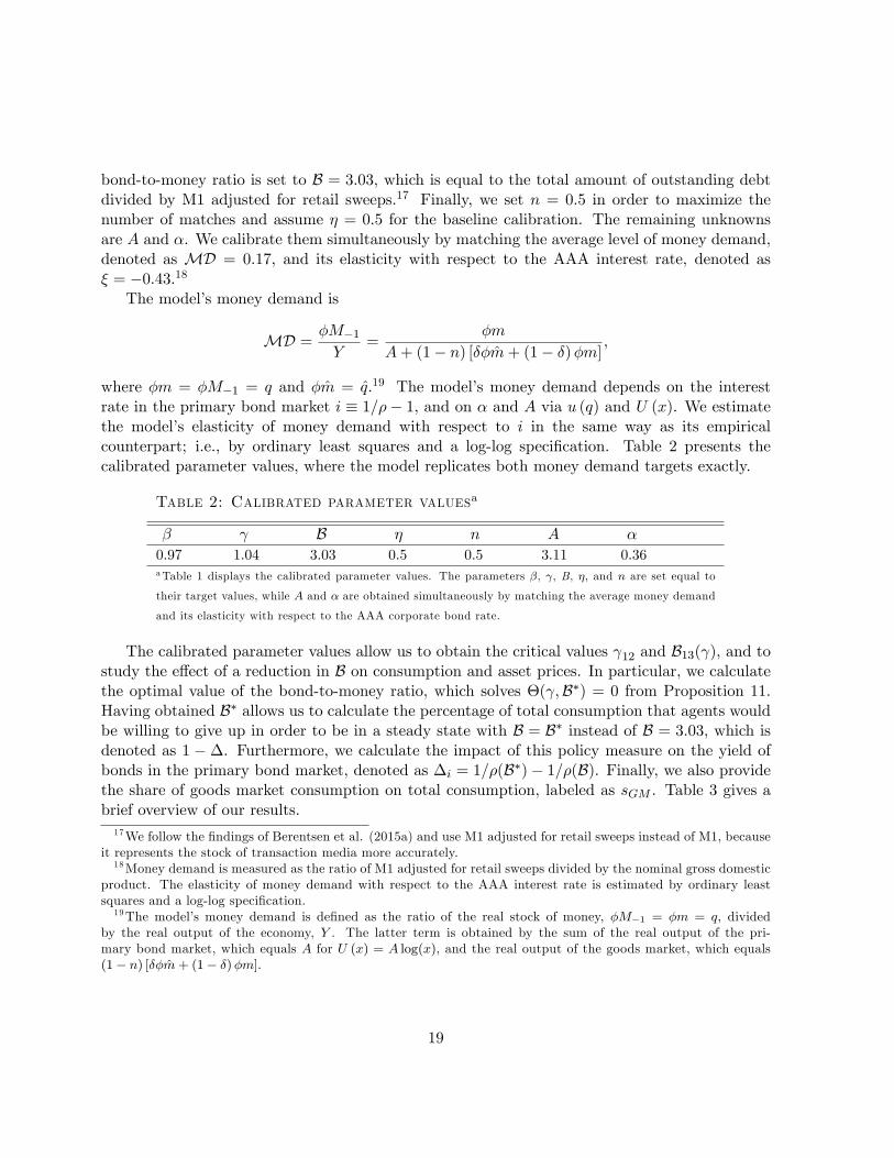
bond-to-money ratio is set to B = 3:03, which is equal to the total amount of outstanding debtdivided by M1 adjusted for retail sweeps.17 Finally, we set n = 0:5 in order to maximize thenumber of matches and assume � = 0:5 for the baseline calibration. The remaining unknownsare A and �. We calibrate them simultaneously by matching the average level of money demand,denoted as MD = 0:17, and its elasticity with respect to the AAA interest rate, denoted as� = �0:43.18
The model�s money demand is
MD = �M�1Y
=�m
A+ (1� n) [��m̂+ (1� �)�m] ;
where �m = �M�1 = q and �m̂ = q̂.19 The model�s money demand depends on the interestrate in the primary bond market i � 1=�� 1, and on � and A via u (q) and U (x). We estimatethe model�s elasticity of money demand with respect to i in the same way as its empiricalcounterpart; i.e., by ordinary least squares and a log-log speci�cation. Table 2 presents thecalibrated parameter values, where the model replicates both money demand targets exactly.
Table 2: Calibrated parameter valuesa
� B � n A �
0.97 1.04 3.03 0.5 0.5 3.11 0.36aTable 1 displays the calibrated parameter values. The parameters �, , B, �, and n are set equal to
their target values, while A and � are obtained simultaneously by matching the average money demand
and its elasticity with respect to the AAA corporate bond rate.
The calibrated parameter values allow us to obtain the critical values 12 and B13( ), and tostudy the e¤ect of a reduction in B on consumption and asset prices. In particular, we calculatethe optimal value of the bond-to-money ratio, which solves �( ;B�) = 0 from Proposition 11.Having obtained B� allows us to calculate the percentage of total consumption that agents wouldbe willing to give up in order to be in a steady state with B = B� instead of B = 3:03, which isdenoted as 1 ��. Furthermore, we calculate the impact of this policy measure on the yield ofbonds in the primary bond market, denoted as �i = 1=�(B�)� 1=�(B). Finally, we also providethe share of goods market consumption on total consumption, labeled as sGM . Table 3 gives abrief overview of our results.17We follow the �ndings of Berentsen et al. (2015a) and use M1 adjusted for retail sweeps instead of M1, because
it represents the stock of transaction media more accurately.18Money demand is measured as the ratio of M1 adjusted for retail sweeps divided by the nominal gross domestic
product. The elasticity of money demand with respect to the AAA interest rate is estimated by ordinary leastsquares and a log-log speci�cation.19The model�s money demand is de�ned as the ratio of the real stock of money, �M�1 = �m = q, divided
by the real output of the economy, Y . The latter term is obtained by the sum of the real output of the pri-mary bond market, which equals A for U (x) = A log(x), and the real output of the goods market, which equals(1� n) [��m̂+ (1� �)�m].
19
Table 3: Calibration resultsa
12 B13( ) B� 1�� �i sGM1.07 0.73 0.50 0.00014 -0.0052 0.11aTable 2 displays the calibration results. The term 12 denotes the critical in�ation rate that separates
the type-I from the type-II equilibrium and the term B13( ) denotes the critical bond-to-money ratio that
separates the type-I from the type-III equilibrium at the calibrated value of = 1:04. The table also shows the
optimal bond-to-money ratio, B�, which is calculated such that �( ;B�) = 0. It also shows the percentage
of total consumption that agents would be willing to give up in order to be in a steady state with B= B�,
instead of B= 3:03, denoted as 1��, and the e¤ect on the yield of bonds of such a policy measure, denotedas �i. Finally, it also shows the size of the goods market, sGM .
Table 3 shows that 12 = 1:07 > 1:04; i.e., that the U.S. economy is in the type-I equilibriumat the calibrated value of . Furthermore, we have B32( ) > B23( ), since � = 0:5 < 2�� = 0:78,and thus there exists an overlapping region supporting the type-II and the type-III equilibriumfor all > 12. We �nd that B� = 0:50, which is signi�cantly lower than its empirical counterpartof B = 3:03. The bene�ts associated with a policy of reducing B to B� are relatively low and inthe region of 0:014 percent of total consumption. However, reducing B to B� has a major impacton the yield of bonds in the primary bond market; i.e., it reduces i � 1=� � 1 by 0:52 percent.Finally, the share of goods market consumption on total consumption is, with 11 percent, in linewith related studies.20
We now investigate how sensitive our results are with respect to the search and bargainingfrictions in the secondary bond market. In order to do this, we provide two robustness-checks.Firstly, we keep n = 0:5 and recalibrate the model for � = (0:1; 0:3; 0:7; 0:9). Secondly, wekeep � = 0:5 and recalibrate the model for n = (0:1; 0:3; 0:7; 0:9). In Figure 4, we show thedevelopment of B� as a function of for the two robustness exercises as compared to the baselinecalibration (solid black line).
Figure 4: B� as a function of 20See, for instance, Lagos and Wright (2005), Aruoba et al. (2011), or Berentsen et al. (2014 and 2015b).
20
The chart on the left-hand side of Figure 4 shows that the lower the bargaining power ofconsumers in the secondary bond market, the higher the optimal bond-to-money ratio. That is,for � = 0:1, we �nd B� = 0:68 at the calibrated value of , while for � = 0:9, we obtain a valueof B� = 0:12.
The chart on the right-hand side of the above �gure shows that if search frictions are low inthe secondary bond market, i.e., if n is high, then the optimal value of B� is also high. Thatis, for n = 0:1, we �nd B� = 0:42 at the calibrated value of , while for n = 0:9, we obtainB� = B23( ) = 1:28. Hence, for n = 0:9, the economy is in a region of the type-II equilibrium,where it is not welfare-improving to reduce B. Furthermore, higher values of n result in lowervalues of 12. Note, however, that the kink in the above �gures does not represent 12. Sincewelfare is continuous in each type of equilibrium and since welfare is maximized (in terms of B) inthe interior of the region of the type-III equilibrium for = 12, then it must also be maximizedin the interior of the region of the type-III equilibrium, when > 12 and is su¢ ciently close to 12 by above continuities. Hence, only when is considerably higher than 12, it is not optimalto reduce B in the type-II equilibrium, such that B� = B23( ).
Figure 5: 1�� as a function of
Figure 5 shows the development of 1 � � as a function of . The left-hand side of Figure5 shows that higher values of � result in higher bene�ts of reducing B to B� in terms of totalconsumption. In particular, for � = 0:1, we �nd 1�� � 0:000 percent at the calibrated value of , while for � = 0:9, we obtain a value of 1 �� = 0:099 percent. Comparing the left-hand sideof Figure 5 to its counterpart in Figure 4 shows clearly that it can be optimal to reduce B in thetype-II equilibrium if is su¢ ciently close to 12. In particular, the kink in Figure 5 represents 12, and the development of 1 �� shows that the bene�ts of reducing B to B� are the highestat = 12 and decreasing thereafter.
The right-hand side of Figure 5 shows that for higher values of n, the bene�ts of reducing Bto B� in terms of total consumption increase up to n = 0:5 and decrease thereafter. In particular,for n = 0:1, we �nd 1 � � � 0:005 percent at the calibrated value of , while for n = 0:7 weobtain a value of 1 �� = 0:012 percent, which is lower than the value obtained for n = 0:5 of1 � � = 0:014 percent. The reason behind this result is that most agents are made worse o¤
21
for high values of n, while only a few passive agents can increase their consumption due to thehigher value of money as a consequence of the reduction in B. For n = 0:9, we �nd that it isoptimal to reduce B only for < 1:01, where 12 = 1:00.
In Figure 6, we show the e¤ect of reducing B to B� on the yield of bonds in the primary bondmarket, �i. Again, we �nd that the e¤ect of reducing B to B� is most pronounced for high valuesof � or intermediate values of n.
Figure 6: �� as a function of
The above analysis shows that a policy measure of reducing B to B� improves the allocationand welfare if the bargaining power of consumers in the secondary bond market is su¢ cientlyhigh. Furthermore, if search frictions are low, reducing B is only bene�cial for low in�ation ratesand the gains in terms of total consumption are low, because most agents are made worse o¤ andonly a few bene�t from the higher value of money.
8.1 Empirical Evidence
In the market for U.S. Treasuries, search frictions are low and mainly caused by delays due to thesearch for suitable counterparties.21 Therefore, our baseline value of n = 0:5 is likely to be toolow. A possibility to obtain a more realistic estimate of n is to replicate the e¤ect on i caused byrecent implementations of QE. D�Amico and King (2013) estimate that the central bank purchasesof U.S. government bonds, which took place in 2009, were successful in reducing yields by around0:3 percent. Thus, we use �i = �0:003 as a target to calibrate n. Furthermore, insights fromexperimental economics indicate that � = 0:5 is a reasonable assumption in bilateral anonymousmeetings.22 Therefore, we stick to the value of � = 0:5 used in the baseline calibration.
21See, for instance, Du¢ e et al. (2005) for a more detailed discussion about search frictions in �nancial marketsor Krishnamurthy (2002) for the empirical price e¤ects of search frictions in the market for U.S. Treasuries.22Forsythe et al. (1994) conduct two experiments of ultimatum (take-it-or-leave-it) and dictator (take-it) games
in the U.S. in 1988. They �nd that if subjects get paid, they tend to act �fairly� and share the pie evenly inthe ultimatum games, which contradicts the subgame perfect Nash equilibrium (which implies an o¤er of 0).Furthermore, the authors �nd that their results are independent of the size of the pie. Roth et al. (1991) conductultimatum games in Israel, Japan, the U.S., and Yugoslavia in 1989 and 1990. They �nd that the proposals made
22
Due to the new target, we need to calibrate one more parameter simultaneously. That is, wecalibrate A, �, and n simultaneously by matching the average level of money demand, MD =0:17, its elasticity with respect to the AAA interest rate, � = �0:43, and the e¤ect of QE on theyield of bonds, �i = �0:003. Table 4 summarizes the calibration results.
n 12 B13( ) B� 1�� �i sGM0.76 1.04 1.18 0.95 0.00002 -0.0040 0.07aTable 4 is Table 3�s counterpart for a calibration that also targets �i in order to estimate n. For a description
of the reported variables, we refer the reader to Table 3.
Following the new calibration procedure, we are still able to hit the money demand targetsperfectly, but the closest we can get to the target of �i is �i = �0:0040. Table 3 shows that theestimate of n increases from n = 0:5 to n = 0:76. This results in an optimal bond-to-money ratioof B� = 0:95, which is nearly twice as high as in the baseline calibration, where we obtained avalue of B� = 0:50. We �nd that 12 = 1:04 and that QE is only welfare-improving for in�ationrates below 4:3 percent. Furthermore, the bene�ts associated with such a policy are low; i.e.,agents are only willing to give up 1 �� = 0:002 percent of total consumption in order to be ina steady state with B = B� instead of B = 3:03.
9 Conclusion
We develop a general equilibrium model, where agents can trade money for government bonds ina secondary �nancial market, which features search and bargaining frictions. The possibility todo so reduces the incentive to self-insure against liquidity shocks, and as a consequence agentsrely on the liquidity provision by other market participants. In such an environment, QE canbe welfare-improving for low in�ation rates. The reason is that such a policy measure reducesthe bond-to-money ratio, which results in a price of bonds above the fundamental value. Hence,bonds become scarce and less attractive, which induces agents to increase their demand for money.In turn, this marginally increases the value of money and so improves the allocation and welfare.
We calibrate the model to U.S. data and �nd that for a realistic parameterization with lowsearch frictions and equally distributed bargaining power among producers and consumers, QEproves competent in reducing the yield of bonds by around 0:40 percent. However, the bene�tsof such a policy measure in terms of total consumption are likely to be small and in the area of0:002 percent. Furthermore, QE is only successful for in�ation rates below 4:3 percent.
by bargainers are the highest in the U.S. and Yugoslavia with a modal proposal of 50 percent of the pie and thelowest in Japan and Israel with a modal proposal of 40 percent of the pie. Furthermore, the authors �nd that thesize of the pie does not a¤ect their results in a meaningful way. Slonim and Roth (1998) conduct an ultimatumgame in the Slovak Republic in 1994. They �nd that subjects o¤er between 41.5 percent and 44 percent and thata bigger size of the pie results in lower o¤ers when players have the possibility to gain experience.
23
10 Appendix - For Online Publication
10.1 Proofs
Proof of Proposition 1. Derivation of (22). Since the short selling constraints (12) are notbinding in a type-I equilibrium, it is obvious from (16) that (22) holds.
Derivation of (23). The marginal value of money of an agent at the beginning of a periodcan be written as follows:
@V1@m
= (1� n)@Vp1
@m+ n
@V c1@m
:
Using (17), we can rewrite the above equation as
@V1@m
= (1� n)���@K
@mc+@V c2@mc
�+ n
��p(1� �)
@K
@mp+@V p2@mp
�;
where
@K
@mc:=@K(mc;mp; bc; bp)
@mcj(mc;mp;bc;bp)=(m;m;b;b);
@K
@mp:=@K(mc;mp; bc; bp)
@mpj(mc;mp;bc;bp)=(m;m;b;b) :
We can use the envelope condition of a consumer in the goods market, (8), to replace @V c2@mc
, and
(11) to replace @V p2@mp
. Furthermore, in a symmetric equilibrium, we have @K@mc
= � � �u0 (q) and@K@mp
= 0, because @q̂@mc
= 0, @q@mc
= 1p = �, @dm@mc
= �1, and @q̂@mp
= @q@mp
= @dm@mp
= 0 with (15).
Using these expressions to replace @K@mc
and @K@mp
and (5) updated one period, we get (23).Derivation of (24). Following the same procedure as in the derivation of (23), we can rewrite
the marginal value of bonds at the beginning of a period as
@V1@b
= (1� n)���@K
@bc+@V c2@bc
�+ n
��p(1� �)
@K
@bp+@V p2@bp
�:
Using (8) to replace @Vc2
@bc, (11) to replace @V
p2
@bp, @K@bp =
@K@bc
= 0, and (5) updated one period, we get(24).Proof of Proposition 2. Derivation of (28). Since the cash-constraint of active and passiveconsumers in the goods market is binding, we have mc + dm = pq̂ for an active consumer andmc = pq for a passive consumer. Furthermore, because active producers are cash-constrainedin the secondary bond market, we have mp = dm = M . Using mp = mc = M and rearrangingterms, we obtain (28).
Derivation of (29). The marginal value of money of an agent at the beginning of a period
24
can be written as
@V1@m
= (1� n)���@K
@mc+@V c2@mc
�+ n
��p(1� �)
@K
@mp+@V p2@mp
�;
where we used (17). We can use the envelope condition of a consumer in the goods market, (8), to
replace @Vc2
@mcand (11) to replace @V
p2
@mp. In a symmetric equilibrium, we have @K
@mc= �u0 (q̂)��u0 (q)
and @K@mp
= �u0 (q̂) � �, because @q̂@mc
= @q@mc
= 1p = �, @dm@mc
= 0, and @q̂@mp
= �, @q@mp
= 0 and@dm@mp
= 1 with (15). Using these expressions to replace @K@mc
and @K@mp
and (5) updated one period,
we get (23).23
Derivation of (30). The derivation of (30) is equal to the derivation of (24) and is not repeatedhere.Proof of Proposition 3. Derivation of (34). Since the bond constraint of active consumers isbinding in the secondary bond market, we have db = b. Since the cash-constraint of active andpassive consumers is binding in the goods market, we have mc + dm = pq̂ and mc = pq. Usingthese expressions and the �rst-order condition of producers in the goods market, p� = 1, in (13),we obtain (34).
Derivation of (35). The marginal value of money of an agent at the beginning of a periodcan be written as
@V1@m
= (1� n)���@K
@mc+@V c2@mc
�+ n
��p(1� �)
@K
@mp+@V p2@mp
�;
where we used (17). We can use the envelope condition of a consumer in the goods market, (8),
equation (25) holds. Thus, if a buyer has a little more (or less) mc, agents will still trade dm = mp. Hence @dm@mc
= 0.
If a producer has a little more (or less) mp, then he will still trade the whole mp. Hence @dm@mp
= 1. @q@mp
= 0 isobvious.24 It is obvious that @q̂
@mp= @q
@mp= @dm
@mp= 0, since q̂, q, and dm do not depend on the producer�s money holdings,
because the producer�s cash constraint is non-binding in the type-III equilibrium.
25
Next, we have to �nd @q̂@mc
and @dm@mc
. By (13), we have
(1� �)�u0(q̂)
@q̂
@mc� u0(q) @q
@mc
�= ���@dm
@mc(41)
and since q̂ = �(mc + dm), q = �mc, we also have
@q̂
@mc= �+ �
@dm@mc
and@q
@mc= �: (42)
By solving the system of equations (41) and (42), we can derive
@q̂
@mc= �
� + (1� �)u0(q)� + (1� �)u0(q̂) ; (43)
@dm@mc
=1� ���
�u0(q̂)
@q̂
@mc� u0(q) @q
@mc
�: (44)
Using (43) and (44) in (40), we have
@K
@mc= u0(q̂)
@q̂
@mc� u0(q) @q
@mc+1� ��
�u0(q̂)
@q̂
@mc� u0(q) @q
@mc
�=
1
�
�u0(q̂)
@q̂
@mc� u0(q) @q
@mc
�=1
�
��u0(q̂)
� + (1� �)u0(q)� + (1� �)u0(q̂) � �u
0(q)
�;
where we have used @q@mc
= �. Using the above equation in (39) and (5) updated one period, weobtain (35).
Derivation of (36). The marginal value of bonds at the beginning of a period can be writtenas
@V1@b
= (1� n)���@K
@bc+@V c2@bc
�+ n
��p(1� �)
@K
@bp+@V p2@bp
�: (45)
By (34), we can �nd
@q̂
@b=
�
(1� �)u0(q̂) + � and@dm@b
=1
(1� �)u0(q̂) + � ,
since B = �b�m =
�bq . Using the above equations to replace
@q̂@bc
and @dm@bc, @q@bc
= 0, and @q̂@bp
= @q@bp
=@dm@bp
= @q@bc
= 0, we obtain
@K
@bc= �
u0(q̂)� 1(1� �)u0(q̂) + � ;
@K
@bp= 0:
26
Using the two above equations in (45), (8) to replace @V c2@bc, (11) to replace @V p2
@bp, and (5) updated
one period, we obtain (36).Proof of Proposition 4. In the type-I equilibrium, agents must hold enough money and bondsto support the optimal amount of consumption for active consumers, u0(q̂) = 1. First, considerthe following system of equations
u0(q̂) = 1;
q̂ = 2q;
�= (1� n)�� + (1� n)(1� ��)u0(q) + n;
with three variables q̂, q, and . Let q̂12, q12, and 12 be the solution of the system of equations.The existence of the solution is immediate. By construction, 12 is the threshold of the in�ationrate at which the cash constraint of active producers is just binding, �mp = �dm. From the proofof proposition 2, we know that q̂ = 2q. Hence � 12 must hold in the type-I equilibrium.
Furthermore, the bond-to-money ratio must be high enough in order to support u0(q̂) = 1.Hence, for a given � 12, consider the following system of equations
u0(q̂) = 1;
Bq = (1� �)[u(q̂)� u(q)] + �(q̂ � q);
�= (1� n)�� + (1� n)(1� ��)u0(q) + n;
with three variables q̂, q, and B. Let q̂13( ), q13( ), and B13( ) be the solution of the system ofequations. The existence of the solution is immediate, since u0 is continuous and u0(1) = 0. Byconstruction, B13( ) is the threshold of the bond-to-money ratio at which the bond constraint ofactive consumers is just binding. Hence, B � B13( ) must hold in the type-I equilibrium.Proof of Proposition 5. First, consider the following system of equations,
with three variables q̂, q, and . Let q̂21, q21, and 21 be the solution of the system of equations.With u0(q̂) = 1, we have
�= (1� n)(1� ��)u0(q) + (1� n)�� + n:
Hence the solution exists, and 21 = 12. By the construction of 21 = 12, it follows that 12 isthe threshold of the in�ation rate at which active consumers can consume the optimal amountof goods, u0(q̂) = 1. Hence � 12 must hold in the type-II equilibrium.
27
In the type-II equilibrium, the bond-to-money ratio must be high enough such that the bondconstraint is not binding in the secondary bond market. Hence, given that � 12, we considerthe following system of equations
with three variables q̂, q, and B. Let q̂23( ), q23( ), and B23( ) be the solution of the system ofequations. The existence of the solution is immediate, since u0 is continuous and u0(0) =1. Byconstruction, B23( ) is the threshold of the bond-to-money ratio at which the bond constraint isjust binding conditional on the given in�ation rate . Hence B > B13( ) must hold in the type-IIequilibrium.Proof of Proposition 6. Case � 12: Given � 12, consider the following system ofequations,
u0(q̂) = 1;
Bq = (1� �)[u(q̂)� u(q)] + �(q̂ � q);
�= (1� n)�u0(q̂)� + (1� �)u
0(q)
� + (1� �)u0(q̂) + (1� n)(1� �)u0(q) + n;
with three variables q̂, q, and B. Let q̂31( ), q31( ), and B31( ) be the solution of the system ofequations. With u0(q̂) = 1, we have
�= (1� n)(1� ��)u0(q) + (1� n)�� + n:
Hence the solution exists, and B31( ) = B13( ). By the construction of B31( ) = B13( ), itfollows that B13( ) is the threshold of the bond-to-money ratio at which active consumers canconsume the optimal amount of goods u0(q̂) = 1. Hence, B � B13( ) must hold in the type-IIIequilibrium conditional on � 12.
Case > 12: Given > 12, consider the system of equations,
q̂ = 2q;
Bq = (1� �) [u(q̂)� u(q)] + �(q̂ � q);
�= (1� n)�u0(q̂)� + (1� �)u
0(q)
� + (1� �)u0(q̂) + (1� n)(1� �)u0(q) + n
with three variables q̂, q, and B. Let q̂32( ), q32( ), and B32( ) be the solution of the system ofequations. The existence of the solution is immediate, since u0 is continuous, lim
q!0(1�n)�u0(2q)�+(1��)u0(2q) =
(1�n)�(1��) 2 R, and u
0(0) =1. By construction, B32( ) is the threshold of the bond-to-money ratio
28
at which the cash constraint in the secondary bond market is also binding. Hence, B < B32( )must hold in the type-III equilibrium conditional on > 12.Proof of Lemma 7. (i): Note that q̂13( ), q13( ), and B13( ) are the solution of the systemof equations
u0(q̂) = 1;
Bq = (1� �)[u(q̂)� u(q)] + �(q̂ � q);
�= (1� n)�� + (1� n)(1� ��)u0(q) + n:
From the last equation, it is easy to see that q13 is decreasing in . From the �rst and the secondequation, we have
@B@q
=(1� �)(�u0(q)� �)
q� (1� �)[u(q̂)� u(q)] + �(q̂ � q)
q2< 0:
Therefore, as increases, q13 decreases and B13( ) increases.(ii): Note that q̂23( ), q23( ), and B23( ) are the solution of the system of equations
The last inequality follows immediately from u00 < 0. Hence q32 is decreasing in . From the �rstand the second equation, we have
@B@q
< 0;
as is shown in (ii). Therefore, as increases, q32 decreases and B32( ) increases.(iv): The proof is immediate by noticing that the following three formulas are identical when
Since by assumption u0(2q)� �u0(q) + � > 0, we have f2(q) > f3(q). Moreover, because
@f2@q
= 2(1� n)�u00(2q) + (1� n)(1� ��)u00(q) < 0;
we must haveq23( ) > q32( ):
Otherwise, we would have a contradiction, � = f2(q23( )) > f3(q32( )) = � .
By (13), the bond-to-money ratio is
B = (1� �)u(2q)� u(q)q
+ �:
Hence, if we di¤erentiate B with respect to q, we obtain
@B@q
=2u0(2q)� u0(q)
q� u(2q)� u(q)
q2< 0;
as we showed in the proof of Lemma 7. Therefore B32( ) > B23( ), because q23( ) > q32( ).Proof of Lemma 9. As > 12 approaches 12, q32( ) <
q�
2 approaches q�
2 . Hence, for agiven a, we have q32( ) > a for a su¢ ciently small . From the previous proof, we have
f2(q)� f3(q) =(1� n)�(1� �)� + (1� �)u0(2q)
�u0(2q)� 1
� �u0(2q)� �u0(q) + �
�:
31
For a small , so for q32( ) > a, we have u0(2q32( )) � �u0(q32( )) + � > 0. Therefore, it holdsthat f2(q32( )) > f3(q32( )). Because also
@f2@q < 0, and
�= f2(q23( )) = f3(q32( )) =
�;
we must haveq23( ) > q32( ):
Otherwise, we would have a contradiction, � = f2(q23( )) > f3(q32( )) = � . At last, we have
@B@q
=2u0(2q)� u0(q)
q� u(2q)� u(q)
q2< 0:
Since q23( ) > q32( ) > a, we must have B32( ) > B23( ).Proof of Lemma 10. As approaches 1, q32( ) approaches zero. Hence for a given a,q32( ) < a for a su¢ ciently large . From the previous proof, we have
f2(q)� f3(q) =(1� n)�(1� �)� + (1� �)u0(2q)
�u0(2q)� 1
� �u0(2q)� �u0(q) + �
�:
For large ; i.e., for q32( ) < a, we have u0(2q32( )) � �u0(q32( )) + � < 0. Therefore, it holdsthat f2(q32( )) < f3(q32( )). Because also
@f2@q < 0, and
�= f2(q23( )) = f3(q32( )) =
�;
we must haveq23( ) < q32( ):
Otherwise, we would have a contradiction, � = f2(q23( )) < f3(q32( )) = � . At last, we have
@B@q
=2u0(2q)� u0(q)
q� u(2q)� u(q)
q2< 0:
Since q23( ) < q32( ) < a, we must have B32( ) < B23( ).Proof of Proposition 11. Consider any ( ;B) that supports the type-III equilibrium. Notethat q̂ = q̂( ;B), q = q( ;B), and qp = qp( ;B) are completely determined by ( ;B) in thetype-III equilibrium, because q̂, q and qp are solutions of the system of equations,
nqp = (1� n) [�q̂ + (1� �)q] (46)
Bq = (1� �) [u(q̂)� u(q)] + �(q̂ � q); (47)
�= (1� n)�u0(q̂)� + (1� �)u
0(q)
� + (1� �)u0(q̂) + (1� n)(1� �)u0(q) + n: (48)
32
By di¤erentiating equation (46) with respect to B, we obtain
n@qp@B = (1� n)
��@q̂
@B + (1� �)@q
@B
�:
Hence, we can simplify (38) as
(1� �)@W@B = (1� n)
���u0(q̂)� 1
� @q̂@B + (1� �)
�u0(q)� 1
� @q@B
�:
By di¤erentiating equation (47) with respect to B, we have
1�n1���( ;B). Thus, if �( ;B) > 0, then welfare will be improved by increasing B, and
if �( ;B) < 0, then welfare will be improved by decreasing B.Proof of Theorem 12. By Proposition 4, < 12, and B > B13( ). Decreasing the bond-to-money ratio B up to B13( ) will not change welfare, since it supports the type-I equilibrium.But at B = B13( ),
The inequality comes from A(q̂; q) > 0, B(q̂; q;B) < 0, and u0(q)�1 > 0. Welfare will be improvedby decreasing B further at B13( ) by Proposition 11.
10.2 Data Source
All the data that we used for the calibration is downloadable from the Federal Reserve Bank ofSt. Louis FRED R database. Table A.1 gives a brief overview of the respective identi�ers.
Table A.1: Data source
Description Identi�er PeriodAAA Moody�s corporate bond AAA 60:Q1-10:Q4Consumer price index CPIAUCSL 60:Q1-10:Q4U.S. total public debt GFDEBTN 66:Q1-10:Q4M1 money stock M1SL 60:Q1-66:Q4M1 sweep-adjusted money stock M1ADJ 67:Q1-10:Q4Nominal GDP GDP 60:Q1-10:Q4
35
Because the time series of the total public debt is only available from 1966:Q1, we con-struct the quarterly data in the period from 1960:Q1 to 1965:Q4 with the data provided byhttp://www.treasurydirect.gov/govt/reports/pd/mspd/mspd.htm. To obtain the quarterly data,we apply the same aggregation method as the Federal Reserve Bank of St. Louis FRED R data-base, which is de�ned as the average of the monthly data. Since the time series of the sweep-adjusted M1 is only available from 1967:Q1, we use the time series of M1 (identi�er M1SL) inthe period from 1960:Q1 to 1966:Q4.
References
[1] Andolfatto, D., 2011, �A Note on the Societal Bene�ts of Illiquid Bonds,�Canadian Journalof Economics, 44, 133-147.
[2] Aruoba, B., Rocheteau, G., and Waller, C., 2007, �Bargaining and the Value of Money,�Journal of Monetary Economics, 54, 2636-2655.
[3] Aruoba, S. B., Waller, C., and Wright, R., 2011, �Money and Capital,�Journal of MonetaryEconomics, 58, 98-116.
[4] Bauer, M., and Neely, C., 2013 �International Channels of the Fed�s Unconventional Mone-tary Policy,�working paper, Federal Reserve Bank of San Francisco.
[5] Berentsen, A., Huber, S., and Marchesiani, A., 2014, �Degreasing the Wheels of Finance,�International Economic Review, 55, 735-763.
[6] Berentsen, A., Huber, S., and Marchesiani, A., 2015a, �Financial Innovations, Money De-mand, and the Welfare Cost of In�ation,�Journal of Money, Credit and Banking, forthcom-ing.
[7] Berentsen, A., Huber, S., and Marchesiani, A., 2015b, �The Societal Bene�ts of a FinancialTransaction Tax,�working paper (�rst version 2014), University of Zürich.
[8] Berentsen, A., and Waller, C., 2011, �Outside Versus Inside Bonds: A Modigliani-MillerType Result for Liquidity Constrained Economies,�Journal of Economic Theory, 146, 1852-1887.
[9] Chun, Y., and Thomson, W., 1988, �Monotonicity properties of bargaining solutions whenapplied to economics,�Mathematical Social Sciences, 15, 11-27.
[10] D�Amico, S., and King, T. B., 2013, �Flow and Stock E¤ects of Large-Scale Asset Purchases:Evidence on the Importance of Local Supply,�Journal of Financial Economics, 108, 425-448.
[11] Du¢ e, D., Gârleanu, N., and Pederson, L. H., 2005, �Over-the-Counter Markets,�Econo-metrica, 73, 1815-1847.
36
[12] Du¢ e, D., Gârleanu, N., and Pederson, L. H., 2008, �Valuation in Over-the-Counter Mar-kets,�Review of Financial Studies, 20, 1865-1900.
[13] Forsythe, R., Horowith, J. L., Savin, N. E., and Sefton, M., 1994, �Fairness in SimpleBargaining Experiments,�Games and Economic Behavior, 6, 347-369.
[14] Gagnon, J., Raskin, M., Remache, J., and Sack, B., 2011, �The Financial Market E¤ectsof the Federal Reserve�s Large-Scale Asset Purchases,� International Journal of CentralBanking, 7, 3-43.
[15] Geromichalos, A., and Herrenbrueck, L., 2014, �Monetary Policy, Asset Prices, and Liquidityin Over-the-Counter Markets,�working paper (�rst version 2012), University of California,Davis.
[16] Geromichalos, A., Herrenbrueck, L., and Salyer, K., 2014, �A Search-Theoretic Model of theTerm Premium,�working paper (�rst version 2013), University of California, Davis.
[17] Gertler, M., and Karadi, P., 2013, �QE 1 vs. 2 vs. 3...: A Framwork for Analyzing Large-ScaleAsset Purchases as a Monetary Policy Tool,� International Journal of Central Banking, 9,5-53.
[18] Greenwald, B., and Stiglitz, J., 1986, �Externalities in Economies with Imperfect Informationand Incomplete Markets,�Quarterly Journal of Economics, 101, 229-264.
[19] Herrenbrueck, L., 2014, �QE and the Liquidity Channel of Monetary Policy,�working paper,Simon Fraser University.
[20] Kalai, E., 1977, �Proportional Solutions to Bargaining Situations: Interpersonal UtilityComparisons,�Econometrica, 45, 1623-1630.
[21] Kocherlakota, N., 1998, �Money Is Memory,�Journal of Economic Theory, 81, 232-251.
[22] Kocherlakota, N., 2003, �Societal Bene�ts of Illiquid Bonds,�Journal of Economic Theory,108, 179-193.
[23] Krishnamurthy, A., 2002, �The Bond/Old-Bond Spread,�Journal of Financial Economics,66, 463-506.
[24] Krishnamurthy, A., and Vissing-Jorgensen, A., 2013, �The Ins and Outs of LSAPs,�workingpaper.
[25] Lagos, R., and Rocheteau, G., 2009, �Liquidity in Asset Markets with Search Frictions,�Econometrica, 77, 403-426.
[26] Lagos, R., Rocheteau, G., and Weill, P., 2011, �Crises and Liquidity in Over-the-CounterMarkets,�Journal of Economic Theory, 146, 2169-2205.
37
[27] Lagos, R., and Wright, R., 2005, �A Uni�ed Framework for Monetary Theory and PolicyEvaluation,�Journal of Political Economy, 113, 463-484.
[28] Rocheteau, G., and Wright, R., 2005, �Money in Competitive Equilibrium, in Search Equi-librium, and in Competitive Search Equilibrium,�Econometrica, 73, 175-202.
[29] Rocheteau, G., and Wright, R., 2013, �Liquidity and Asset Market Dynamics,�Journal ofMonetary Economics, 60, 275-294.
[30] Roth, A. E., Prasnikar, V., Okuno-Fujiwara, M., Zamir, S., 1991, �Bargaining and Mar-ket Behaviour in Jerusalem, Ljublijana, Pittsburgh, and Tokyo: An Experimental Study,�American Economic Review, 81, 1068-1095.
[31] Shi, S., 2006, �Viewpoint: A Microfoundation of Monetary Economics,�Canadian Journalof Economics, 39, 643-688.
[32] Slonim, R., and Roth, A. E., 1998, �Learning in High Stakes Ultimatum Games: An Exper-iment in the Slovak Republic,�Econometrica, 66, 569-596.
[34] Williamson, S., 2012, �Liquidity, Monetary Policy, and the Financial Crisis: A New Mone-tarist Approach,�American Economic Review, 102, 2570-2605.
[35] Williamson, S., 2014a, �Scarce Collateral, the Term Premium, and QE,� working paper,Federal Reserve Bank of St. Louis.
[36] Williamson, S., 2014b, �Central Bank Purchases of Private Assets,�working paper, FederalReserve Bank of St. Louis.