Statistics & Risk Modeling 28, 359–387 (2011) / DOI 10.1524/strm.2011.1094 c Oldenbourg Wissenschaftsverlag, M¨ unchen 2011 Central limit theorem for the integrated squared error of the empirical second-order product density and goodness-of-fit tests for stationary point processes Lothar Heinrich and Stella Klein Received: January 12, 2011; Accepted: September 8, 2011 Summary: Spatial point processes are mathematical models for irregular or random point patterns in the d-dimensional space, where usually d = 2 or d = 3 in applications. The second-order product density and its isotropic analogue, the pair correlation function, are important tools for analyzing stationary point processes. In the present work we derive central limit theorems for the integrated squared error (ISE) of the empirical second-order product density and for the ISE of the empirical pair correlation function when the observation window expands unboundedly. The proof techniques are based on higher-order cumulant measures and the Brillinger-mixing property of the underlying point processes. The obtained Gaussian limits are used to construct asymptotic goodness-of-fit tests for checking point process hypotheses even in the non-Poissonian case. 1 Introduction An important aim of point process statistics is to find a mathematical model that gives a satisfactory description of an observed point pattern. With such models one can, for instance, draw conclusions about properties of certain materials or tissues. For stationary and isotropic point processes (PPes) mainly second-order statistics such as Ripley’s K -function and the pair correlation function are used for verifying or reject- ing hypothetical PP models by visual inspection or simulation tests, see e.g. Baddeley et al. [1], Cressie [4], Diggle [7], Illian et al. [15], and Stoyan et al. [21]. Often these investigations focus on complete spatial randomness, see e.g. Grabarnik and Chiu [8], Ho and Chiu [14], and Zimmerman [24]. Most tests used in applications are based on heuristic considerations rather than on test statistics with known distribution derived from specified model assumptions. This is mainly due to the complexity of the most PP models in R d with d ≥ 2 caused by the intrinsic spatial and stochastic dependencies. In the AMS 2000 subject classification: Primary: 60G55, 62M30, 60F05; Secondary: 62G10, 62G20 Key words and phrases: Second-order analysis of point processes, pair correlation function, Brillinger-mixing, cumulant measures, asymptotic variance, model specification test
Central limit theorem for the integratedsquared error of the empirical second-orderproduct density and goodness-of-fit tests forstationary point processes
Lothar Heinrich and Stella Klein
Received: January 12, 2011; Accepted: September 8, 2011
Summary: Spatial point processes are mathematical models for irregular or random point patternsin the d-dimensional space, where usually d = 2 or d = 3 in applications. The second-orderproduct density and its isotropic analogue, the pair correlation function, are important tools foranalyzing stationary point processes. In the present work we derive central limit theorems for theintegrated squared error (ISE) of the empirical second-order product density and for the ISE ofthe empirical pair correlation function when the observation window expands unboundedly. Theproof techniques are based on higher-order cumulant measures and the Brillinger-mixing propertyof the underlying point processes. The obtained Gaussian limits are used to construct asymptoticgoodness-of-fit tests for checking point process hypotheses even in the non-Poissonian case.
1 IntroductionAn important aim of point process statistics is to find a mathematical model that givesa satisfactory description of an observed point pattern. With such models one can,for instance, draw conclusions about properties of certain materials or tissues. Forstationary and isotropic point processes (PPes) mainly second-order statistics such asRipley’s K -function and the pair correlation function are used for verifying or reject-ing hypothetical PP models by visual inspection or simulation tests, see e.g. Baddeleyet al. [1], Cressie [4], Diggle [7], Illian et al. [15], and Stoyan et al. [21]. Often theseinvestigations focus on complete spatial randomness, see e.g. Grabarnik and Chiu [8],Ho and Chiu [14], and Zimmerman [24]. Most tests used in applications are based onheuristic considerations rather than on test statistics with known distribution derived fromspecified model assumptions. This is mainly due to the complexity of the most PP modelsin Rd with d ≥ 2 caused by the intrinsic spatial and stochastic dependencies. In the
AMS 2000 subject classification: Primary: 60G55, 62M30, 60F05; Secondary: 62G10, 62G20Key words and phrases: Second-order analysis of point processes, pair correlation function, Brillinger-mixing,cumulant measures, asymptotic variance, model specification test
360 Heinrich -- Klein
present paper we will use the second-order product density and its isotropic analogue, thepair correlation function, to construct goodness-of-fit tests for a wide class of stationaryPPes. Based on a single realization of a PP in some observation window, which is assumedto expand in all directions, we study the integrated squared error (ISE) of kernel-typeestimators of the second-order product density (and of the pair correlation function inthe isotropic case), where in both cases the integration stretches over a freely selectablebounded set K . The asymptotic behavior of the ISE of probability density estimators hasbeen studied e.g. by Hall [10] who derived central limit theorems (CLTs) for the ISE forindependent random variables and by Takahata and Yoshihara [23] who extended Hall’sresult to absolutely regular random sequences. We will derive CLTs for the ISE of ourkernel-type estimators in the setting of Brillinger-mixing PPes. The Gaussian limits willsolely depend on the intensity, the second-order product density resp. pair correlationfunction of the underlying hypothetical PP, and on the chosen kernel function as well ason the set K . This allows the construction of distribution-free testing procedures.
Next we introduce some basic notions. Let [M,M] denote the measurable space of alllocally finite counting measures on the d-dimensional Euclidean space Rd equipped withits σ-algebra Bd of Borel sets. A point process PP on Rd is defined to be a measurablemapping � from a probability space [�,A,P] into [M,M]. Throughout in this paper weassume that � is simple, i.e. P
(�({x}) ≤ 1 for all x ∈ Rd
) = 1, and strictly stationary,see Guan [9] for a test on stationarity. Let E and Var denote expectation and variance,respectively, with respect to P. Let P = P ◦ �−1 denote the probability measure on[M,M] induced by � and we will briefly write � ∼ P. If E�k(B) < ∞ for all boundedBorel sets B, then there exist the k-th-order factorial moment measure α(k) and thek-th-order factorial cumulant measure γ (k) on [Rdk,Bdk] defined by
α(k)( k×
j=1B j
):=
∫
M
∑∗
x1,...,xk∈ψ
k∏
j=1
1B j (x j)P(dψ) = E( ∑∗
x1,...,xk∈�
k∏
j=1
1B j (x j))
and
γ (k)( k×
j=1B j
):=
k∑
�=1
(−1)�−1(� − 1)!∑
K1∪···∪K�={1,...,k}
�∏
j=1
α(#K j)( ×
k j ∈K j
Bk j
)
with B1, . . . , Bk ∈ Bdk, respectively. Here the abbreviation “x ∈ ψ” means “x ∈ Rd :ψ({x}) > 0”. Further,
∑∗ denotes summation over summands with index tuples havingpairwise distinct components. The sum
∑K1∪···∪K�={1,...,k}
is taken over all partitions of the set
{1, 2, . . . , k} into � disjoint non-empty subsets K j and #K j denotes the cardinality ofK j . If � ∼ P is stationary with intensity λ = E�([0, 1)d) > 0 the k-th-order reduced
factorial moment measure α(k)red is implicitly defined by the disintegration
α(k)( k×
j=1B j
)= λ
∫
Bk
α(k)red
( k−1×j=1
(B j − x))
dx,
CLT for the integrated squared error and goodness-of-fit tests 361
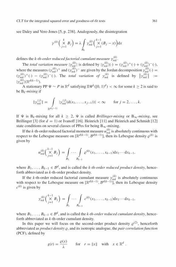
see Daley and Vere-Jones [5, p. 238]. Analogously, the disintegration
γ (k)( k×
j=1B j
)= λ
∫
Bk
γ(k)red
( k−1×j=1
(B j − x))
dx
defines the k-th-order reduced factorial cumulant measure γ(k)red .
The total variation measure |γ (k)red | is defined by |γ (k)
red |(·) = (γ(k)red )+(·) + (γ
(k)red )−(·),
where the measures (γ(k)red )+ and (γ
(k)red )− are given by the Jordan decomposition γ
(k)red (·) =
(γ(k)red )+(·) − (γ
(k)red )−(·). The total variation of γ
(k)red is defined by
∥∥γ (k)red
∥∥ :=|γ (k)
red |(Rd(k−1)).A stationary PP � ∼ P in Rd satisfying E�k([0, 1)d) < ∞ for some k ≥ 2 is said to
be Bk-mixing if
‖γ ( j)red ‖ =
∫
Rd( j−1)
|γ ( j)red (d(x1, . . . , x j−1))| < ∞ for j = 2, . . . , k.
If � is Bk-mixing for all k ≥ 2, � is called Brillinger-mixing or B∞-mixing, seeBrillinger [3] (for d = 1) or Ivanoff [16]. Heinrich [11] and Heinrich and Schmidt [12]state conditions on several classes of PPes for being B∞-mixing.
If the k-th-order reduced factorial moment measure α(k)red is absolutely continuous with
respect to the Lebesgue measure on [Rd(k−1),Bd(k−1)], then its Lebesgue density (k) isgiven by
α(k)red
( k−1×j=1
B j
)=
∫
B1
· · ·∫
Bk−1
(k)(x1, . . . , xk−1)dx1 · · ·dxk−1,
where B1, . . . , Bk−1 ∈ Bd , and is called the k-th-order reduced product density, hence-forth abbreviated as k-th-order product density.
If the k-th-order reduced factorial cumulant measure γ(k)red is absolutely continuous
with respect to the Lebesgue measure on [Rd(k−1),Bd(k−1)], then its Lebesgue densityc(k) is given by
γ(k)red
( k−1×j=1
B j
)=
∫
B1
· · ·∫
Bk−1
c(k)(x1, . . . , xk−1)dx1 · · ·dxk−1,
where B1, . . . , Bk−1 ∈ Bd , and is called the k-th-order reduced cumulant density, hence-forth abbreviated as k-th-order cumulant density.
In this paper we will focus on the second-order product density (2), henceforthabbreviated as product density , and its isotropic analogue, the pair correlation function(PCF), defined by
g(r) = (x)
λfor r = ‖x‖ with x ∈ Rd .
362 Heinrich -- Klein
The remaining part of the paper is organized as follows. Section 2 introduces the estimatorsfor the product density and the PCF and their ISEs. In Section 3 we formulate someauxiliary results and the CLTs for the ISEs. In Section 4 these CLTs are applied toconstruct asymptotic goodness-of-fit tests. The proofs of the results in Section 3 areshifted to Section 5.
2 Integrated squared errors of the empirical productdensity and the empirical pair correlation function
In this section we define the announced empirical counterparts of the product density
and the PCF g together with their ISEs with respect to bounded domains of integration.Further, we formulate three basic conditions needed to obtain the asymptotic results inthe next section.
Let ρ(W ) := sup{r ≥ 0 : b(x, r) ⊂ W, x ∈ Rd} denote the radius of the inball ofW ⊂ Rd , where b(x, r) := {y ∈ Rd : ‖y − x‖ ≤ r} is the ball with radius r ≥ 0 centeredat x ∈ Rd . Let |.| denote the Lebesgue measure on [Rd,Bd] and let ωd = |b(o, 1)| denotethe volume of the unit ball in Rd . The following condition is needed either for s = d ors = 1.
Condition C(s)
(i) The sequence of observation windows (Wn)n∈N is an increasing sequence of convexand compact sets in Rd with ρ(Wn) −−−→
n→∞ ∞,
(ii) the sequence of bandwidths (bn)n∈N is a decreasing sequence of positive real num-bers such that bn −−−→
n→∞ 0 and bsn|Wn | −−−→
n→∞ ∞, and
(iii) the kernel function ks : Rs → R is bounded with bounded support and symmetric(i.e., ks(x) = ks(−x) for x ∈ Rs) such that
∫Rs ks(x)dx = 1.
The following kernel-type estimator for the product density goes back to Krickeberg[19]. The problem of consistency of the estimator (2.1) as n → ∞ has been studied inJolivet [18] and Heinrich and Liebscher [13] for various modes of convergence.
Definition 2.1 Let (Wn)n∈N, (bn)n∈N and kd satisfy Condition C(d). Let the PP � ∼ Pin Rd be stationary with product density . For λ(t) at any t ∈ Rd define the estimator
n(t) = 1
bdn|Wn |
∑∗
x1,x2∈�
1Wn (x1)kd
( x2 − x1 − t
bn
). (2.1)
Definition 2.2 Let (Wn)n∈N, (bn)n∈N and k1 satisfy Condition C(1). Let the PP � ∼ P inR
d be stationary and isotropic with PCF g. For λ2g(r) at any r > 0 define the estimator
gn(r) = 1
bn|Wn |dωd
∑∗
x1,x2∈�
1Wn(x1)
‖x2 − x1‖d−1 k1
(‖x2 − x1‖ − r
bn
). (2.2)
CLT for the integrated squared error and goodness-of-fit tests 363
Since En(t) = λ∫Rd k(y)(bn y + t)dy and Egn(r) = λ2
∫ ∞−r/bn
k(y)g(bn y + r)dy,the above estimators are asymptotically unbiased in all points of continuity of and g,respectively. Note that x2 in the definition of the above estimators may lie outside Wn .Thus, information from outside the sampling window is needed. The results in Sections 3and 4 also hold for the edge-corrected versions of n(t) and gn(r), where the ratio1Wn (x1)/|Wn | must be replaced by the ratio 1Wn(x1)1Wn(x2)/|(Wn − x1) ∩ (Wn − x2)|.For a discussion of various empirical PCFs with regard to bias and variance the reader isreferred to Stoyan and Stoyan [22]. The ISE of the empirical product density (2.1) withrespect to a bounded set K ∈ Bd satisfying
∫K (t)dt > 0 is defined by
In(K ) =∫
K
(n(t) − λ(t)
)2dt . (2.3)
Likewise, the ISE of the empirical PCF (2.2) with respect to a bounded set K ∈ B1
satisfying inf K > 0 and∫
K g(r)dr > 0 is defined by
Jn(K ) =∫
K
(gn(r) − λ2g(r)
)2dr . (2.4)
Condition C�(K ) Let K ∈ Bd be bounded such that∫
K (t)dt > 0 and, for some ε > 0,
(i) the first-order partial derivatives ∂i, i = 1, . . . , d, of are uniformly Lipschitz-continuous on Kε := {x + y : x ∈ K, ‖y‖ < ε}, i.e. |∂i(t) − ∂i(s)| ≤ L‖t − s‖for s, t ∈ Kε, and
(ii) the third- and fourth-order cumulant densities c(3) and c(4) exist and satisfy
supu,v∈Kε
|c(3)(u, v)| < ∞ and supu,v∈Kε
∫
Rd
|c(4)(u, w, v + w)|dw < ∞.
Condition Cg(K ) Let K ∈ B1 be bounded such that inf K > 0,∫
K g(r)dr > 0, and
(i) for some ε > 0, the first derivative g′ exists and is uniformly Lipschitz-continuousin Kε := {x + y : x ∈ K, |y| < ε}, i.e. |g′(t) − g′(s)| ≤ L|t − s| for s, t,∈ Kε, and
(ii) the third- and fourth-order cumulant densities c(3) and c(4) exist and satisfy
supu,v∈Rd:
‖u‖,‖v‖∈Kε
|c(3)(u, v)| < ∞ and supu,v∈Rd:
‖u‖,‖v‖∈Kε
∫
Rd
|c(4)(u, w, v + w)|dw < ∞.
Remark 2.3 Besides the stationary Poisson process � ∼ �λ with intensity λ (andg(r) ≡ 1, (t) ≡ λ) there are quite a few other B∞-mixing PPes satisfying C(K ) or
364 Heinrich -- Klein
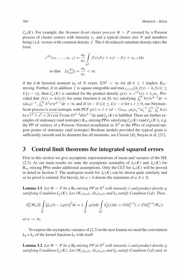
Cg(K ). For example, the Neyman–Scott cluster process � ∼ P covered by a Poissonprocess of cluster centers with intensity λc and a typical cluster size N and membersbeing i.i.d. vectors with common density f . The k-th reduced cumulant density takes theform
c(k)(x1, . . . , xk−1) = αk
α1
∫
Rd
f(y) f(y + x1)· · · f(y + xk−1)dy
so that ‖γ (k)red‖ = αk
α1< ∞
if the k-th factorial moment αk of N exists. ENk < ∞ for all k ≥ 1 implies B∞-mixing. Further, if in addition f is square-integrable and max1≤i≤d
∣∣∂i f(y) − ∂i f(x)∣∣ ≤
L‖y − x‖, then C(K ) is satisfied for the product density (x) = c(2)(x) + λcα1. Pro-vided that f(x) = h(‖x‖) for some function h on [0,∞) satisfying
∫ ∞0 h(r)rd−1dr =
(dωd )−1,∫ ∞
0 h2(r)rd−1dr < ∞ and |h′(t) − h′(s)| ≤ L|t − s| for s, t ≥ 0, our Neyman–Scott process is even isotropic with PCF g(r) = 1 + (d − 1)ωd−1α2λ
−1c α−2
1
∫ ∞0
∫ π
0 h(s)
h(√
r2 + s2 + 2rs cos ϑ)(sin ϑ)d−2dϑsd−1ds and Cg(K ) is fulfilled. There are further ex-amples of stationary (and isotropic) B∞-mixing PPes satisfying C(K ) (and Cg(K )), e.g.the PP of vertices of a Poisson–Voronoi tessellation in Rd or the PPes of exposed tan-gent points of stationary (and isotropic) Boolean models provided the typical grain issufficiently smooth and its diameter has all moments, see Cressie [4], Stoyan et al. [21].
3 Central limit theorems for integrated squared errorsFirst in this section we give asymptotic representations of mean and variance of the ISE(2.3). As our main results we state the asymptotic normality of In(K ) and Jn(K ) forB∞-mixing PPes under additional assumptions. Only the CLT for In(K ) will be provedin detail in Section 5. The analogous result for Jn(K ) can be shown quite similarly andso its proof is omitted. For brevity, let a ∧ b denote the minimum of a, b ∈ R.
Lemma 3.1 Let � ∼ P be a B4-mixing PP in Rd with intensity λ and product density
satisfying Condition C(K ). Let (Wn)n∈N, (bn)n∈N and kd satisfy Condition C(d). Then,
bdn|Wn|E
∫
K
(n(t) − λ(t)
)2dt = λ
∫
K
(t)dt∫
Rd
k2d(x)dx +O(bd∧2
n ) +O(bd+4n |Wn |)
as n → ∞.
To express the asymptotic variance of (2.3) in the next lemma we need the convolutionkd ∗ kd of the kernel function kd with itself.
Lemma 3.2 Let � ∼ P be a B8-mixing PP in Rd with intensity λ and product density
satisfying Condition C(K ). Let (Wn)n∈N, (bn)n∈N and kd satisfy Condition C(d) and, in
CLT for the integrated squared error and goodness-of-fit tests 365
addition, bd+4n |Wn| −−−→
n→∞ 0. Then,
Var(√
bdn|Wn |
∫
K
(n(t) − λ(t)
)2dt)
−−−→n→∞ σ2
with
σ2 := 2λ2(∫
K
2(t)dt +∫
K∩(−K )
2(t)dt
)∫
Rd
(kd ∗ kd)2(t)dt > 0 .
Now we state a CLT for the ISE of the product density estimator in the setting of B∞-mixing PPes. This result will be proved in Section 5 based on the “method of moments”,see Billingsley [2], by showing that the cumulants of order k ≥ 3 of the scaled ISE (2.3)converge to zero.
The notationD−−−→
n→∞ stands for weak convergence and N (μ, σ2) denotes a Gaussian
random variable with mean μ ∈ R and variance σ2 > 0.
Theorem 3.3 Let � ∼ P be a B∞-mixing PP in Rd with intensity λ and product density satisfying Condition C(K ). Let all cumulant densities c(k), k ≥ 2, exist. Let (Wn)n∈N,(bn)n∈N and kd satisfy Condition C(d) and, in addition, bd+4
n |Wn | −−−→n→∞ 0. Then,
√bd
n|Wn|(In(K ) − EIn(K )
) D−−−→n→∞ N (0, σ2)
with variance σ2 > 0 from Lemma 3.2.
To be complete we present an asymptotic expression for the mean of the ISE (2.4)followed by the CLT for the centered and scaled term Jn(K ) revealing its asymptoticvariance τ2.
Lemma 3.4 Let � ∼ P be a B4-mixing and isotropic PP in Rd with intensity λ and PCFg satisfying Condition Cg(K ). Let (Wn)n∈N, (bn)n∈N and k1 satisfy Condition C(1). Then,
bn|Wn |E∫
K
(gn(r) − λ2g(r)
)2dr = 2λ2
∫
K
g(r)
dωdrd−1 dr∫
R
k21(x)dx + O(bn) +O(b5
n |Wn|)
as n → ∞.
Theorem 3.5 Let � ∼ P be a B∞-mixing and isotropic PP in Rd with intensity λ andPCF g satisfying Condition Cg(K ). Let all cumulant densities c(k), k ≥ 2, exist. Let(Wn)n∈N, (bn)n∈N and k1 satisfy Condition C(1) and, in addition, b5
n|Wn | −−−→n→∞ 0. Then,
√bn|Wn|
(Jn(K ) − EJn(K )
) D−−−→n→∞ N (0, τ2)
366 Heinrich -- Klein
with
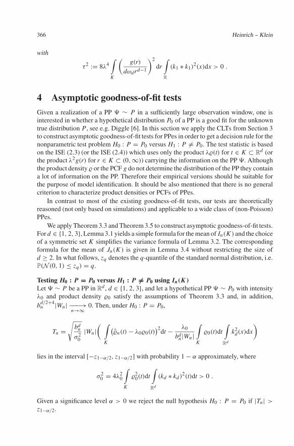
τ2 := 8λ4∫
K
(g(r)
dωdrd−1
)2
dr∫
R
(k1 ∗ k1)2(x)dx > 0 .
4 Asymptotic goodness-of-fit testsGiven a realization of a PP � ∼ P in a sufficiently large observation window, one isinterested in whether a hypothetical distribution P0 of a PP is a good fit for the unknowntrue distribution P, see e.g. Diggle [6]. In this section we apply the CLTs from Section 3to construct asymptotic goodness-of-fit tests for PPes in order to get a decision rule for thenonparametric test problem H0 : P = P0 versus H1 : P �= P0. The test statistic is basedon the ISE (2.3) (or the ISE (2.4)) which uses only the product λ(t) for t ∈ K ⊂ Rd (orthe product λ2g(r) for r ∈ K ⊂ (0,∞)) carrying the information on the PP �. Althoughthe product density or the PCF g do not determine the distribution of the PP they containa lot of information on the PP. Therefore their empirical versions should be suitable forthe purpose of model identification. It should be also mentioned that there is no generalcriterion to characterize product densities or PCFs of PPes.
In contrast to most of the existing goodness-of-fit tests, our tests are theoreticallyreasoned (not only based on simulations) and applicable to a wide class of (non-Poisson)PPes.
We apply Theorem 3.3 and Theorem 3.5 to construct asymptotic goodness-of-fit tests.For d ∈ {1, 2, 3}, Lemma 3.1 yields a simple formula for the mean of In(K ) and the choiceof a symmetric set K simplifies the variance formula of Lemma 3.2. The correspondingformula for the mean of Jn(K ) is given in Lemma 3.4 without restricting the size ofd ≥ 2. In what follows, zq denotes the q-quantile of the standard normal distribution, i.e.P(N (0, 1) ≤ zq) = q.
Testing H0 : P = P0 versus H1 : P �= P0 using In(K )
Let � ∼ P be a PP in Rd , d ∈ {1, 2, 3}, and let a hypothetical PP � ∼ P0 with intensityλ0 and product density 0 satisfy the assumptions of Theorem 3.3 and, in addition,bd/2+4
n |Wn| −−−→n→∞ 0. Then, under H0 : P = P0,
Tn =√
bdn
σ20
|Wn |( ∫
K
(n(t) − λ00(t)
)2dt − λ0
bdn|Wn |
∫
K
0(t)dt∫
Rd
k2d(x)dx
)
lies in the interval [−z1−α/2, z1−α/2] with probability 1 − α approximately, where
σ20 = 4λ2
0
∫
K
20(t)dt
∫
Rd
(kd ∗ kd )2(t)dt > 0 .
Given a significance level α > 0 we reject the null hypothesis H0 : P = P0 if |Tn| >
z1−α/2.
CLT for the integrated squared error and goodness-of-fit tests 367
Testing H0 : P = P0 versus H1 : P �= P0 using Jn(K )
Let � ∼ P be a PP in Rd and let a hypothetical PP � ∼ P0 with intensity λ0 and PCF g0
satisfy the assumptions of Theorem 3.5 and, in addition, b9/2n |Wn | −−−→
n→∞ 0.
Then, under H0 : P = P0,
Tn =√
bn
τ20
|Wn|( ∫
K
(gn(r) − λ2
0g0(r))2dr − 2λ2
0
bn|Wn |∫
K
g0(r)
dωdrd−1 dr∫
R
k21(x)dx
)
belongs in the interval [−z1−α/2, z1−α/2] with probability 1 − α approximately, where
τ20 = 8λ4
0
∫
K
(g0(r)
dωdrd−1
)2
dr∫
R
(k1 ∗ k1)2(x)dx > 0 .
Given a significance level α > 0 we reject the null hypothesis H0 : P = P0 if |Tn| >
z1−α/2.Concerning the applicability of our asymptotic goodness-of-fit tests there are several
issues that have to be studied carefully. Firstly, there is the problem of how to choose thebandwidths, the kernel function, and the set K . The choice of the kernel function is – asknown from probability density estimation – of comparatively minor relevance. The setK should be chosen according to the Conditions C(K ) or Cg(K ) such that “particularfeatures” of the hypothesized product density or PCF are captured. The selection of thebandwidths bn relative to the size of Wn is a delicate problem: So far an optimal bandwidthcan be determined at most up to some constant so that, for a given point pattern, thereis no rule of thumb to find its value. Another question concerns how large has to be thewindow Wn to get a good normal approximation. Answers to these questions may befound through large-scale simulation studies which are subject of further research. Theaccuracy in the CLT can be affected besides window size |Wn | and bandwidth bn byseveral other factors such as the distribution P of �, λ, , kd , and K . Given a hypotheticaldistribution P0 and the associated test problem H0 : P = P0 versus H1 : P �= P0 itis obvious how to investigate the type-I error (that is, the probability of rejecting thenull hypothesis when it is actually true) by simulation studies. The type-II error (thatis, the probability of not rejecting the null hypothesis when the alternative hypothesisis actually true) is difficult to handle since the true distribution P can differ from P0 inmany different ways. Hence the type-II error can only be studied for some special cases.For example, if P = �λ and P0 = �λ0 with λ �= λ0, an investigation of the type-IIerror for different combinations of λ and λ0 is a sensitivity analysis of the test procedurewith respect to the intensity of the underlying Poisson process. Another example of sucha sensitivity analysis is given in Grabarnik and Chiu [8] who consider the null hypothesisof a Poisson process and the alternative hypothesis of a mixture of a conditional StraussPP and Matern’s cluster process.
Note that an unknown intensity λ0 cannot be replaced in In(K ) by an estimator (λ0)nsince the weak limit of
∫K (n(t) − (λ0)n0(t))2dt may differ from that in Theorem 3.3.
However, the intensity λ0 occurring in the mean and the variance of Tn can be replacedby a consistent estimator (λ0)n due to Slutsky’s theorem, see Billingsley [2]. Anotherproblem might arise if the product density 0 of the hypothetical PP �0 is unknown.
368 Heinrich -- Klein
Nevertheless, our tests can be applied if 0 is replaced by an estimator (0)n obtainedfrom simulated realizations of � ∼ P0 in Wn . Analogous considerations apply to thegoodness-of-fit test based on the PCF g.
5 Proofs of the resultsThe normal convergence of the centered and suitably scaled ISE In(K ) is proved byshowing that all cumulants of order k ≥ 3 converge to zero. Lemmas 5.1 and 5.2 yielda representation formula for the cumulants of the ISE (2.3). This representation can alsobe used to obtain the asymptotic variance of (2.3). To begin with we derive the asymptoticrepresentation of the mean EIn(K ).
Proof of Lemma 3.1: By Fubini’s theorem and the definition of Var(n(t)
),
E
∫
K
(n(t) − λ(t)
)2dt =
∫
K
Var(n(t)
)dt +
∫
K
(En(t) − λ(t)
)2dt.
For the second summand it is easily seen that
bdn|Wn|
∫
K
(En(t) − λ(t)
)2dt = bdn|Wn|λ2
∫
K
( ∫
Rd
((t + bnz) − (t)
)kd(z)dz
)2dt.
Using the Taylor expansion of (·) in t = (t1, . . . , td ) with ∂i = ∂∂ti
for brevity, we getthat
(t + bnz) = (t) + bn
d∑
i=1
zi∂i(t) + bn Rn(t, z), (5.1)
where Rn(t, z) = ∑di=1 zi
(∂i(t + θibnz) − ∂i(t)
)for some θi ∈ [0, 1], i = 1, . . . , d.
The symmetry of the kernel function kd and the smoothness condition C(K )(i) on ∂i
entail that∣∣∣∫
Rd
((t + bnz) − (t)
)kd(z)dz
∣∣∣ = bn
∣∣∣∫
Rd
Rn(t, z)(t)kd(z)dz∣∣∣
≤ b2ndL
∫
Rd
‖z‖2|kd(z)|dz.
Therefore,
bdn|Wn |
∫
K
(En(t) − λ(t)
)2dt = O(bd+4n |Wn |) as n → ∞.
Next we prove the asymptotic relation
bdn|Wn|
∫
K
Var(n(t)
)dt = λ
∫
K
(t)dt∫
Rd
k2d(x)dx +O(bd∧2
n ).
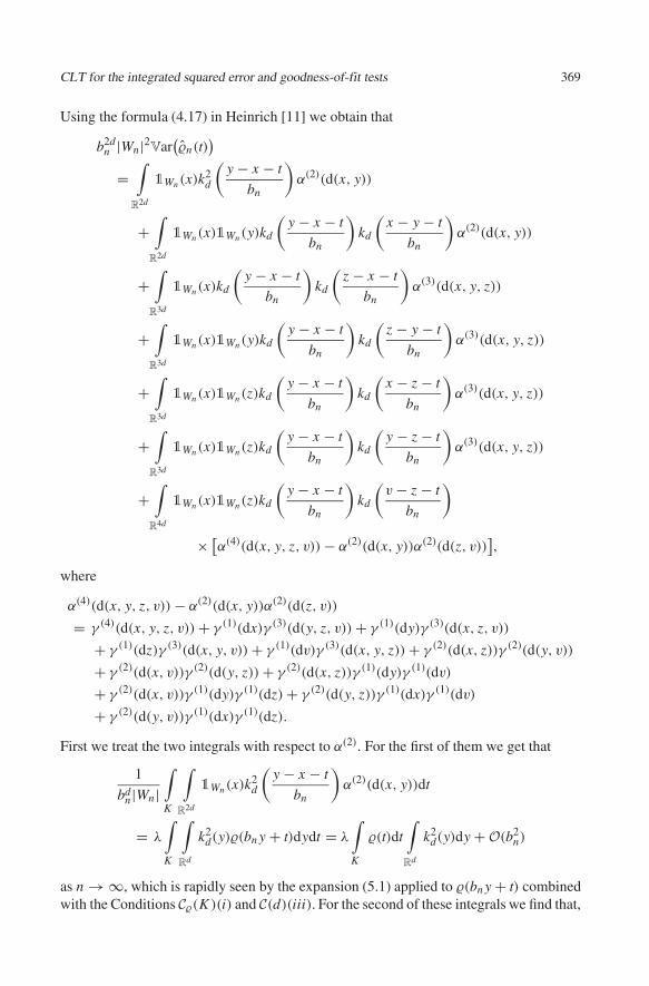
CLT for the integrated squared error and goodness-of-fit tests 369
Using the formula (4.17) in Heinrich [11] we obtain that
b2dn |Wn|2Var
(n(t)
)
=∫
R2d
1Wn(x)k2d
(y − x − t
bn
)α(2)(d(x, y))
+∫
R2d
1Wn(x)1Wn(y)kd
(y − x − t
bn
)kd
(x − y − t
bn
)α(2)(d(x, y))
+∫
R3d
1Wn(x)kd
(y − x − t
bn
)kd
(z − x − t
bn
)α(3)(d(x, y, z))
+∫
R3d
1Wn(x)1Wn(y)kd
(y − x − t
bn
)kd
(z − y − t
bn
)α(3)(d(x, y, z))
+∫
R3d
1Wn(x)1Wn(z)kd
(y − x − t
bn
)kd
(x − z − t
bn
)α(3)(d(x, y, z))
+∫
R3d
1Wn(x)1Wn(z)kd
(y − x − t
bn
)kd
(y − z − t
bn
)α(3)(d(x, y, z))
+∫
R4d
1Wn(x)1Wn(z)kd
(y − x − t
bn
)kd
(v − z − t
bn
)
× [α(4)(d(x, y, z, v)) − α(2)(d(x, y))α(2)(d(z, v))
First we treat the two integrals with respect to α(2). For the first of them we get that
1
bdn|Wn |
∫
K
∫
R2d
1Wn (x)k2d
(y − x − t
bn
)α(2)(d(x, y))dt
= λ
∫
K
∫
Rd
k2d(y)(bn y + t)dydt = λ
∫
K
(t)dt∫
Rd
k2d(y)dy + O(b2
n)
as n → ∞, which is rapidly seen by the expansion (5.1) applied to (bn y + t) combinedwith the Conditions C(K )(i) and C(d)(iii). For the second of these integrals we find that,
370 Heinrich -- Klein
as n → ∞,
1
bdn|Wn |
∫
K
∫
R2d
1Wn(x)1Wn(y)kd
(y − x − t
bn
)kd
(x − y − t
bn
)α(2)(d(x, y))dt
= bdnλ
∫
Rd
∫
Rd
|Wn ∩ (Wn − bn y − bnt)||Wn | kd(y)kd(y − 2t)(bn y + bnt)1K (bnt)dydt
= O(bdn )
The latter relation is justified by the continuity of in Kε if o ∈ K – otherwise the integralvanishes eventually.
Next we consider the integrals with respect to the third-order factorial moment mea-sure α(3). The first of these integrals can be rewritten as follows:
This asymptotic order is seen by applying the dominated convergence theorem and usingthe boundedness of the function kd and of the set K combined with the continuity of c(2)
and supu,v∈Kε|c(3)(u, v)| < ∞ for some ε > 0. By similar arguments we can show the
asymptotic order of the other integrals with respect to the factorial moment measure α(3)
to be O(bdn ), too.
Finally, let us consider the integrals with respect to the factorial cumulant measuresoccurring in the decomposition of α(4) − α(2) × α(2). Due to the finiteness of the totalvariations ‖γ (2)
red‖ and ‖γ (3)red‖ the asymptotic order of the integrals with respect to γ (2) and
γ (3) is easily seen to be O(bdn ). The integral with respect to γ (4) is
1
bdn|Wn |
∫
R5d
1K (t)1Wn (x)1Wn(z)kd
(y − x − t
bn
)kd
(v − z − t
bn
)γ (4)(d(x, y, z, v))dt
= bdnλ
∫
R4d
|Wn ∩ (Wn − z)||Wn | 1K (t)kd(y)kd(v)c
(4)(bn y + t, z, bnv + z + t)dydzdvdt.
CLT for the integrated squared error and goodness-of-fit tests 371
In view of supu,v∈Kε
∫Rd |c(4)(u, w, v + w)|dw < ∞ for some ε > 0 and Condition C(d)
we see that the integral in the last line is bounded as n −−−→n→∞ ∞. Summarizing all above
terms completes the proof of Lemma 3.1. �
The below Lemma 5.1 yields a representation formula for the cumulants of linearcombinations of random multiple sums over the atoms of the PP � ∼ P,
�(pi)( fi) :=∑
x1,...,x pi ∈�
fi(x1, . . . , x pi ) for pi ≥ 1 and i ∈ I = {1, . . . , k}, (5.2)
as sum of so-called “indecomposable” integrals with respect to the cumulant measuresof �. Such integrals do not factorize into two or more integrals. Note that the ISE In(K )
can be rewritten as linear combinations of two multiple sums (5.2) with p1 = 4, p2 = 2,see Lemma 5.2.
To be precise in what follows we give a rigorous definition of decomposability. Letfi : Rdpi → R be Borel-measurable functions such that E
∣∣�(pi )( fi)∣∣k < ∞ for i ∈ I
and define the mixed moment M(�(p1)( f1), . . . ,�
(pk)( fk)) = E[∏k
i=1 �(pi)( fi)].
For any T ⊆ I , q ∈ {1, . . . , pT } with pT = ∑i∈T pi , r ∈ {1, . . . , q}, and for
decompositionsPT = {P1, . . . , Pq} of {1, . . . , pT } andQ = {Q1, . . . , Qr } of {1, . . . , q}we define the integral
IPT ,Q( fi : i ∈ T )
:=∫
Rdq
q∏
b=1
∏
a∈Pb
1{xa=zb} fi1 (x1, . . . , x pi1) fi2 (x pi1 +1, . . . , x pi1 +pi2
)
×· · · × fi#T
(x∑#T−1
j=1 pi j +1, . . . , x pT
) r∏
c=1
γ (#Qc)(d(zq, q ∈ Qc)
),
where {i1, . . . , i#T } = T with 1 ≤ i1 < i2 < · · · < i#T ≤ k. The elements of a setPb are the indices of the arguments of the functions fi1 , . . . , fi#T that are identical anddistinct from all the arguments in every other set Pc �= Pb. In the above-mentionedintegral this is indicated by the term
∏qb=1
∏a∈Pb
1{xa=zb}. In case of T = I , the integralIPI ,Q( f1, . . . , fk) is equal to
∫
Rdq
q∏
b=1
∏
a∈Pb
1{xa=zb} f1(x1, . . . , x p1) × · · ·
× fk(x∑k−1
i=1 pi+1, . . . , x pI
) r∏
c=1
γ (#Qc)(d(zq, q ∈ Qc)
).
The mixed moment M(�(p1)( f1), . . . ,�
(pk)( fk))
can be expressed in terms of factorialmoment measures respectively factorial cumulant measures in following way:
pI∑
q=1
∑
P1∪···∪Pq={1,...,pI }
∫
Rdq
q∏
b=1
∏
a∈Pb
1{xa=zb} f1(x1, . . . , x p1) × · · ·
× fk(x∑k−1
i=1 pi, . . . , x pI
)α(q)(d(z1, . . . , zq))
372 Heinrich -- Klein
=pI∑
q=1
∑
P1∪···∪Pq={1,...,p}
q∑
r=1
∑
Q1∪···∪Qr={1,...,q}
∫
Rdq
q∏
b=1
∏
a∈Pb
1{xa=zb} f1(x1, . . . , x p1) × · · ·
× fk(x∑k−1
i=1 pi+1, . . . , x pI
) r∏
c=1
γ (#Qc)(d(zq, q ∈ Qc)
),
see Krickeberg [19] for explicit relationships between moment measures, factorial mo-ment and factorial cumulant measures of point processes. With the above notation wemay write
M(�(p1)( f1), . . . ,�
(pk)( fk)) =
pI∑
q=1
∑
P1∪···∪Pq={1,...,pI }
q∑
r=1
∑
Q1∪···∪Qr={1,...,q}
IPI ,Q( f1, . . . , fk). (5.3)
Let {T1, T2} be a decomposition of the index set I = {1, . . . , k}. An integralIPI ,Q( f1, . . . , fk) is decomposable with respect to the decomposition {T1, T2} if thereexist a decomposition P(1) of {1, . . . , pT1}, a decomposition P(2) of {1, . . . , pT2}, q1 ∈{1, . . . , pT1} and q2 ∈ {1, . . . , pT2} with q1 + q2 = q, and decompositions Q(1) of{1, . . . , q1} and Q(2) of {1, . . . , q2} such that
IPI ,Q( f1, . . . , fk) = IPT1 ,Q(1)( fi : i ∈ T1) · IPT2 ,Q(2)( fi : i ∈ T2).
An integral is called decomposable if there exists a nontrivial decomposition {T1, T2} ofI (with T1, T2 �= ∅) such that this integral is decomposable with respect to {T1, T2}. Anintegral which is not decomposable with respect to any nontrivial decomposition {T1, T2}is called indecomposable.
The following lemma is the key in applying the “method of moments” to prove CLTsfor random sums taken over p-tuples of atoms of a point process. Whereas cumulantsof simple sums (with p = 1, also known as shot-noise processes) are tightly connectedwith the probability generating functional of � ∼ P, see Heinrich and Schmidt [12],the treatment of the case p ≥ 2 is much more sophisticated, see Jolivet [17]. OurLemma 5.1 generalizes Jolivet’s approach to linear combinations of multiple sums whichlater in Lemma 5.2 leads a representation of the k-th cumulant of In(K ) as sum ofindecomposable integrals. Let �k(X) = Cumk(X, . . . , X) denote the k-th cumulant ofa random variable X, where Cumk(X1, . . . , Xk) denotes the mixed cumulantof the randomvector (X1, . . . , Xk) defined by
Cumk(X1, . . . , Xk) = ∂k
∂s1 · · ·∂sklogE exp{s1 X1 + · · · + sk Xk}
∣∣∣s1=···=sk=0
.
Lemma 5.1 Let the sums �(pi)( fi) defined by (5.2) for some PP � ∼ P on Rd
satisfy max1≤i≤ j E∣∣�(pi )( fi)
∣∣k < ∞ for fixed j, k ∈ N. Then, for any coefficientsc1, . . . , c j ∈ R,
�k
( j∑
i=1
ci�(pi)( fi)
)= k!
∑
k1+···+k j =kk1,...,k j ≥0
ck11 . . . . . c
k jj
k1. . . . . k j ! μ∗k1,...,k j
CLT for the integrated squared error and goodness-of-fit tests 373
with terms μ∗k1,...,k j
that can be expressed by the sum
( p1k1+···+p j k j∑
q=1
∑
P1∪···∪Pq={1,...,p1k1+···+p j k j }
q∑
r=1
∑
Q1∪···∪Qr={1,...,q}
)∗IPI ,Q( f1, . . . , f1︸ ︷︷ ︸
k1
, . . . , f j , . . . , f j︸ ︷︷ ︸k j
),
(5.4)where the summation (· · · )∗ is taken only over the indecomposable integrals.
Proof: By the multi-linearity, symmetry, and homogeneity of the mixed cumulants weget that
, . . . ,�(p j )( f j), . . . ,�(p j )( f j)︸ ︷︷ ︸
k j
)(5.5)
for fixed k1, . . . , k j ≥ 0 with k1 + · · · + k j = k, we use the ideas developed in Jolivet[17] and Leonov and Shiryaev [20]. Next define the sums �i = �(pi)(gi) by
gi =
⎧⎪⎪⎪⎪⎨
⎪⎪⎪⎪⎩
f1 for i ∈ {1, . . . , k1},f2 for i ∈ {k1 + 1, . . . , k1 + k2},
...
f j for i ∈ {k1 + . . . + k j−1 + 1, . . . , k},
and consider the mixed moment M(�1, . . . ,�k) = E[∏k
i=1 �i
]. A well-known rela-
tionship between mixed moments and mixed cumulants, see e.g. Leonov and Shiryaev[20], yields
Cumk(�1, . . . ,�k) = M(�1, . . . ,�k) −k∑
j=2
∑
I1∪···∪I j =I
j∏
i=1
Cum#Ii (�a : a ∈ Ii)
= �indec + �dec − C,
374 Heinrich -- Klein
where∑
I1∪···∪I j =I runs over all decompositions of I = {1, . . . , k} into nonempty setsI1, . . . , I j and the sum �dec stretches over all decomposable integrals in the expansion(5.3) applied to M(�1, . . . ,�k). Further, the sum
is taken over all indecomposable integrals in the expansion (5.3) applied toM(�1, . . . ,�k), and
C =k∑
j=2
∑
I1∪···∪I j =I
j∏
i=1
Cum#Ii (�a : a ∈ Ii) .
For j ∈ {2, . . . , k} and a fixed decomposition {I1, . . . , I j } of I = {1, . . . , k}, a summand∏ j
i=1 Cum#Ii (�a : a ∈ Ii) of C factorizes with respect to a decomposition {T1, T2} of Iif, for each i = 1, . . . , j , we have either Ii ⊆ T1 or Ii ⊆ T2, that is, if the summand canbe written as
j∏
i=1
Cum#Ii (�a : a ∈ Ii) =j∏
i=1Ii ⊆T1
Cum#Ii (�a : a ∈ Ii) ·j∏
i=1Ii⊆T2
Cum#Ii (�a : a ∈ Ii).
Note that due to j ≥ 2 each summand∏ j
i=1 Cum#Ii (�a : a ∈ Ii) factorizes with respectto at least one nontrivial decomposition {T1, T2} of I .
Let PI be the distribution of the vector (�1, . . . ,�k) which is determined by thedistribution P of the PP �. For any J ⊆ I , let PJ be the distribution of the vector (�a)a∈J .Each summand in C that factorizes with respect to a fixed decomposition {T1, T2} of I iscompletely determined by the marginal distributions PT1 and PT2 . The same is true foreach integral term of the sum �dec that is decomposable with respect to {T1, T2}.
Let {T (1)1 , T (1)
2 } be an arbitrarily fixed decomposition of I. The sum over the summands
of �dec that are decomposable with respect to {T (1)1 , T (1)
2 } is denoted by �(1)dec, and the
sum over the summands of C that factorize with respect to {T (1)1 , T (1)
cumulant on the left-hand side of (5.7) disappears and the mixed moment M(�1, . . . , �k),in view of
M(�1, . . . , �k) = E[ k∏
i=1
�i
]= E
[ ∏
i∈T (1)1
�i
]· E
[ ∏
i∈T (1)2
�i
]= �
(1)dec,
is decomposable with respect to the decomposition {T (1)1 , T (1)
2 } so that �indec = 0 and�(1) = 0.
Finally, the independence of(�a : a ∈ T (1)
1
)and
(�a : a ∈ T (1)
2
)implies Cum#J(�a :
a ∈ J ) = 0 for any J ⊆ I with J ∩ T (1)1 �= ∅ and J ∩ T (1)
2 �= ∅. Since each summandin C(1) contains a factor of this type, we obtain that C(1) = 0. This altogether combinedwith equation (5.7) proves (5.6) giving the equality
Cumk(�1, . . . ,�k) = �indec + �(1) − C(1).
Now we go through all possible decompositions of I in this manner. Since every summandof �dec is decomposable with respect to some decomposition of I and every summand ofC factorizes with respect to some decomposition of I , this yields
�dec = C or equivalently Cumk(�1, . . . ,�k) = �indec.
In summary we finally arrive at (5.5) and the proof of Lemma 5.1 is complete. �
The cumulants of the ISE In(K ) can be represented by a sum of indecomposableand irreducible integrals which will be shown in Lemma 5.2. First we give a definitionof an irreducible integral. This definition is closely related to the particular shape of thefunctions
f1(x1, x2, x3, x4) (5.8)
= 1Wn (x1)1Wn(x3)1{x1 �=x2,x3 �=x4}∫
K
kd
( x2 − x1 − t
bn
)kd
( x4 − x3 − t
bn
)dt
and
f2(x1, x2) = 1Wn (x1)1{x1 �=x2}∫
K
kd
( x2 − x1 − t
bn
)λ(t)dt. (5.9)
376 Heinrich -- Klein
An integral IP,Q( f1, . . . , f1︸ ︷︷ ︸k− j
, f2, . . . , f2︸ ︷︷ ︸j
), j = 0, . . . , k − 1, with P = {P1, . . . , Pq}
and Q = {Q1, . . . , Qr}, see (5.4), is reducible if there are indices a, b ∈ {1, . . . , q},c, d ∈ {1, . . . , r}, and an odd number i ∈ {1, . . . , 4k−4 j} such that Pa = {i}, Pb = {i+1},and Qc = {a, b} or Qc = {a} and Qd = {b}. In other words, a reducible integral containsone of the terms
∫
R2d
f1(xi, xi+1, x, y)γ (2)(d(xi, xi+1)),
∫
R2d
f1(x, y, xi, xi+1)γ(2)(d(xi, xi+1)),
∫
R2d
f1(xi, xi+1, x, y)γ (1)(dxi)γ(1)(dxi+1),
or∫
R2d
f1(x, y, xi, xi+1)γ(1)(dxi)γ
(1)(dxi+1),
with x, y �∈ {xi, xi+1}, and the remaining functions contain neither xi nor xi+1. We willcall this term the reducible part of the integral. An integral can have more than onereducible part. An integral that is not reducible is called irreducible. For instance, theintegral
I{{1},{2},{3,5},{4,6}},{{1,2},{3,4}
}( f1, f2)
=∫
R2d
∫
R2d
f1(z1, z2, z3, z4) f2(z3, z4)γ(2)(d(z1, z2))γ
(2)(d(z3, z4))
is reducible with reducible part∫
R2d
f1(z1, z2, z3, z4)γ(2)(d(z1, z2)), whereas the integral
I{{1,5},{2},{3,6},{4}},{{1,2},{3,4}
}( f1, f2)
=∫
R2d
∫
R2d
f1(z1, z2, z3, z4) f2(z1, z3)γ(2)(d(z1, z2))γ
(2)(d(z3, z4))
is irreducible.Now recall the sum of indecomposable integrals μ∗
k− j, j , j = 0, . . . , k defined in(5.4). We denote the sum of irreducible integrals in μ∗
k− j, j by μ∗∗k− j, j , j = 0, . . . , k and
we will write μ∗∗ak−( j+r), j+r with a = 1, . . . , r for the term obtained from μ∗∗
k−( j+r), j+r by
replacing a instances of f2 with f2, where the function f2 is given by
f2(x, y) := 1Wn (x)
∫
K
[kd
(y − x − t
bn
)λ
( ∫
Rd
Rn(t, z)kd(z)dz
)]dt, (5.10)
where Rn(t, z) is defined by (5.1). Thus, μ∗∗ak−( j+r), j+r contains only j + r − a instances
of f2.
CLT for the integrated squared error and goodness-of-fit tests 377
Now we can state the lemma yielding a representation of the k-th cumulant of the ISE(2.3) in terms of indecomposable and irreducible integrals for k ≥ 2.
Lemma 5.2 For fixed k ≥ 2 let � ∼ P be a B4k-mixing PP in Rd with intensity λ > 0and product density . Further, let the conditions C(K )(i) and C(d)(iii) be satisfied. Thenthe k-th cumulant of the ISE (2.3) takes the form
�k(In(K )) =k∑
j=0
(k
j
)2 jb j
n(bdn|Wn |) j−2kμ
∗∗ jk− j, j .
Proof: In the first part of the proof we apply Lemma 5.1 in order to express the k-thcumulant by a sum of indecomposable integrals. Due to the smoothness conditions on theproduct density this representation can be further simplified. This is shown in the secondpart of the proof.
By the semi-invariance of cumulants the k-th cumulant �k(In(K )
)coincides with the
k-th cumulant of the integral∫
K
(2
n(t) − 2λ(t)n(t))dt for k ≥ 2.
I Representation of the k-th cumulant by indecomposable integralsThe integral
∫K
(2
n(t) − 2λ(t)n(t))dt can be rewritten as
∑
x1,x2,x3,x4∈�x1 �=x2,x3 �=x4
(bdn|Wn |)−21Wn(x1)1Wn(x3)
×∫
K
kd
(x2 − x1 − t
bn
)kd
(x4 − x3 − t
bn
)dt
−∑∗
x1,x2∈�
2(bdn|Wn|)−11Wn (x1)
∫
K
kd
(x2 − x1 − t
bn
)λ(t)dt
= c1
∑
x1,x2,x3,x4∈�
f1(x1, x2, x3, x4) + c2
∑
x1,x2∈�
f2(x1, x2),
with functions f1 and f2 given by (5.8) and (5.9), respectively, and coefficients c1 =(bd
n|Wn |)−2 and c2 = −2(bdn|Wn |)−1. By our assumptions the moments
E
∣∣∑x1,x2,x3,x4∈� f1(x1, x2, x3, x4)
∣∣k and E∣∣∑
x1,x2∈� f2(x1, x2)∣∣k are finite. Hence, we
may apply Lemma 5.1 so that �k(In(K )) can be written as sum of indecomposableintegrals
�k(In(K )) =k∑
j=0
(k
j
)(−1) j2 j(bd
n|Wn |) j−2kμ∗k− j, j . (5.11)
II Representation of the cumulants by indecomposable and irreducible integralsThe special form of the functions f1 and f2 allows a further simplification of the rep-resentation for the k-th cumulant given in (5.11). This simplification is based on the
378 Heinrich -- Klein
approximate identity∫
R2d
f1(x1, x2, x3, x4)α(2)(d(x1, x2)) =
∫
R2d
f1(x3, x4, x1, x2)α(2)(d(x1, x2))
≈ bdn|Wn| f2(x3, x4) (5.12)
for x3, x4 �∈ {x1, x2}, which implies the reducible integrals of μ∗k,0 (except for the error
terms) and integrals in μ∗k−�,�, � = 1, . . . , k, to cancel.
More precisely we start by combining two reducible integrals in μ∗k− j, j , j = 0, . . . ,
k − 1. These integrals differ only by their reducible parts, in two possible ways. Eitherthe two integrals’ reducible parts are∫
R2d
f1(xi, xi+1, x, y)γ (2)(d(xi, xi+1)) and∫
R2d
f1(xi, xi+1, x, y)γ (1)(dxi)γ(1)(dxi+1)
or they are∫
R2d
f1(x, y, xi, xi+1)γ(2)(d(xi, xi+1)) and
∫
R2d
f1(x, y, xi, xi+1)γ(1)(dxi)γ
(1)(dxi+1).
The sum of these two reducible integrals in μ∗k− j, j is hence an integral which emerges
from either of the two aforementioned integrals by replacing the respective reducibleparts by
∫
R2d
f1(xi, xi+1, x, y)α(2)(d(xi, xi+1))
or∫
R2d
f1(x, y, xi, xi+1)α(2)(d(xi, xi+1)),
(5.13)
depending on the above distinction. If the integral has more than one reducible part,then we iterate the above procedure, eventually obtaining an irreducible integral. In thefollowing, we will only consider irreducible integrals and integrals which arise from theabove-mentioned combination and summation of reducible integrals. The latter integralsare also called reducible parts. Now we simplify one of the reducible parts in (5.13) ofa reducible integral by disintegration and Taylor expansion, that is,
∫
R2d
1Wn (xi)1Wn(x)
∫
K
kd
(xi+1 − xi − t
bn
)kd
(y − x − t
bn
)dtα(2)(d(xi, xi+1))
= bdn|Wn |1Wn(x)
∫
K
kd
(y − x − t
bn
)λ
( ∫
Rd
kd(xi+1)(bnxi+1 + t)dxi+1
)dt
= bdn|Wn | f2(x, y) + bnbd
n |Wn| f2(x, y)
CLT for the integrated squared error and goodness-of-fit tests 379
with f2(x, y) defined in (5.10). Here we have used the symmetry of the function kd so thatonly (t) and the error term Rn(t, z) remain from the Taylor expansion. In the following wewill refer to the above simplification by disintegration and Taylor expansion as reductionof the integral. Note that the uniform Lipschitz-continuity of the partial derivatives of
yields the upper bound
|Rn(t, z)| ≤d∑
i=1
zi |∂i(t + θibnz) − ∂i(t)| ≤ bndL‖z‖2 . (5.14)
An integral in μ∗k− j, j is called r-reducible if it can be reduced exactly r times (that is,
if reduction as defined above can be applied exactly r times), with r ∈ {0, . . . , k − j}.Reducing an r-reducible integral r times yields a sum of two parts. The first part is anintegral in μ∗∗
k−( j+r), j+r multiplied by (bdn|Wn|)r while the second part is a sum of integrals
containing the error terms from all Taylor expansions performed in the reductions. Notethat within this iterative scheme reductions can also be applied to error terms obtained fromearlier reductions. We illustrate this procedure by an example involving three reductionsof a 3-reducible integral in μ∗
n → ∞. For integrals in μ∗∗02,0 containing an integration with respect to γ (5), γ (6), γ (7) and
γ (8), this is due to the finiteness of these measures’ total variation. For the other integralsone uses the assumptions on the cumulant densities up to order four or the finiteness ofthe total variations
∥∥γ(k)red
∥∥, k = 2, 3, 4. For example, if we do not assume the existenceof the fourth-order cumulant density, the integral
∥∥ < ∞ for k = 2, . . . , 6, the bound(5.14) of the error term Rn(t, z) occurring in the function f2, and the properties ofthe function kd . Plugging in these relations on the right-hand side (5.17) leads to theasymptotic representation
bdn|Wn|2 �2(In(K )) = 2λ2
∫
Rd
(kd ∗ kd)2(t)dt
(∫
K
2(t)dt +∫
K∩(−K )
2(t)dt
)
+O(bd∧2n ) +O((bd
n |Wn|)−1) + O(bd+4n |Wn |),
which together with bd+4n |Wn | −−−→
n→∞ 0 implies the assertion of Lemma 3.2. �
Proof of Theorem 3.3: Together with Lemma 3.2 we prove asymptotic normality byshowing that the k-th cumulant of
√bd
n|Wn |In(K ) converges to zero for all k ≥ 3.In Lemma 5.2 we have shown a representation of the k-th cumulant of In(K ) by
indecomposable and irreducible integrals. Now we will show that the k-th cumulant of√
bdn|Wn |In(K ) is of order O
((bd
n)k/2−1 + b4+ k
2 dn |Wn |) as n → ∞ for k ≥ 2. For this
purpose we have to find the asymptotic order of the terms μ∗∗ jk− j, j for j = 0, . . . , k. It is
essential that the integrals in μ∗∗ jk− j, j are neither decomposable nor reducible.
Consider an integral IP,Q(.) in μ∗∗ jk− j, j , j = 0, . . . , k, see (5.4). Let V be the set of
integration variables occurring in the integral and define the set of argument pairs
V := {{v,w} ⊆ V : the integrand of IP,Q(.) contains
a term f1(v,w, ·, ·), a term f1(·, ·, v,w), or a term f2(v,w)}.
CLT for the integrated squared error and goodness-of-fit tests 383
Now we define a linkage relation on V. Two argument pairs {v,w}, {x, y} ∈ V are said tobe linked (notation: {v,w} � {x, y}) if at least one of the following conditions is satisfied:
(i) The argument pairs {v,w}, {x, y} have a common element, that is, {v,w} ∩ {x, y}�= ∅.
(ii) The integral IP,Q(.) involves an integration γ (i)(d(v1, . . . , vi )) for some i ≥ 2 andsome v1, . . . , vi ∈ V such that {v,w}∩{v1, . . . , vi} �= ∅ and {x, y}∩{v1, . . . , vi } �=∅.
(iii) The integral IP,Q(.) involves an integration γ (1)(dv0)γ(i)(d(v1, . . . , vi)) for some
i ≥ 1 and v0, . . . , vi ∈ V such that {v,w} ∩ {v0, . . . , vi } �= ∅ and {x, y} ∩{v0, . . . , vi} �= ∅.
Note that the relation � is reflexive and symmetric.The maximal asymptotic order of each integration of linked argument pairs with �
arguments isO((bd
n)� �2 �|Wn |). After reduction of the factorial cumulant measures we make
use of the existence of the cumulant densities. There are at least � �2� kernel functions kd. By
substitution of the arguments of the kernel functions kd we get a factor bdn for each function.
Furthermore there is exactly one variable occurring only in the indicator functions 1Wn
(this is due to the integral’s indecomposability and irreducibility). Integration over thisvariable yields the factor |Wn |. Because of the boundedness of the total variations theintegrals over the cumulant densities are also bounded. Therefore we obtain the order
O((bdn )� �
2 �|Wn|) for each integration over � linked argument pairs. Note that withoutthe existence of the cumulant densities one can only derive the order O(|Wn |). Fordetermining the order of the whole integral we also have to take into account that someof the arguments t of the functions 1K (t) can be substituted, where each substitutionproduces a factor bd
n . Thus the highest-order terms are those in which as many argumentpairs as possible are not linked.
We will now use the concept of a cyclic linkage. Consider a product
m∏
i=1
f1(pi, qi)
occurring in the integrand of IP,Q(·) and involving the argument pairs p1, q1, . . . , pm, qm∈ V. (Here f1(p, q) with argument pairs p = {u, v}, q = {x, y} is understood asf1(u, v, x, y).) This product is said to be cyclically linked if there are an enumera-tion r1, . . . , r2m of {p1, q1, . . . , pm, qm} and a permutation π of {1, . . . , m} such that{r2i−1, r2i} = {pπ(i), qπ(i)} for all i = 1, . . . , m and such that
r2i � r2i+1mod2m for all i ∈ {1, . . . , m}is an exhaustive list of the links between the argument pairs p1, q1, . . . , pm, qm .
We will now investigate the highest-order terms in μ∗∗ jk− j, j for j = 0, . . . , k. Let
j = 0. Then the integrands of all highest-order integrals in μ∗∗0k,0 are cyclically linked. As
Taking into account the continuity of the cumulant density c(2) in Kε for some ε > 0we obtain that the above integral has the asymptotic order O
((bd
n )2k−1|Wn |k). Similararguments apply to the other terms in μ∗∗
k,0.
Now let j = 1. Then each integrand of a highest-order term in μ∗∗1k−1,1 is a product
of two parts: First, a cyclically linked product of k − 1 instances of f1, and second, oneinstance of the function f2 whose argument pair is linked to at least one argument pair
CLT for the integrated squared error and goodness-of-fit tests 385
from the first part. One of these highest-order integrals is
By applying disintegration and substitution as above and making use of the bound(5.14) for |Rn(t, z)|, we find the above integral to have the asymptotic orderO(bn(bd
n)2k−2|Wn |k−1). Quite the same arguments apply to the remaining integrals.
Next let j = 2. Then each integrand of a highest-order term in μ∗∗2k−2,2 is a product of
two parts: First, a cyclically linked product of k −2 instances of f1, and second, a productof two instances of the function f2 whose argument pairs are both linked to argumentpairs from the first part. For example, the integral
dn )2k−2|Wn |k−1) and hence one of the highest-order terms
for the case j = 2.For j = 3, . . . , k − 1 one obtains the asymptotic order O(b j
n(bdn )2k− j |Wn|k− j+1) by
analogous considerations.Finally, in the case j = k all integrands of the integrals in μ∗∗k
0,k are products of k
instances of the function f2. Since these integrals are indecomposable the argument pairsoccurring in the integrand can be enumerated as p1, . . . , pk such that pi � pi+1 fori = 1, . . . , k − 1. Hence the term μ∗∗k
0,k is of order O(bkn(bd
n)k|Wn |).Altogether we have
μ∗∗0k,0 = O((bd
n )2k−1|Wn |k), μ∗∗1k−1,1 = O(bn(bd
n)2k−2|Wn|k−1),
andμ
∗∗ jk− j, j = O(b j
n(bdn )2k− j |Wn|k− j+1) for j = 2, . . . , k.
Together with Lemma 5.2 the k-th cumulant hence satisfies
�k(In(K )) = O(b−dn |Wn|−k) + 2kO(b2−d
n |Wn |−k) +k∑
j=2
(k
j
)2 jO(b2 j
n |Wn |1−k).
Hence, we get �k(√
bdn|Wn |In(K )
) = O((bdn)k/2−1 + b
4+ k2 d
n |Wn |) for k ≥ 2. By theassumption bd+4
n |Wn | −−−→n→∞ 0 it follows that �k
(√bd
n |Wn|In(K )) −−−→
n→∞ 0 for k ≥ 3.
This terminates the proof of Theorem 3.3. �
386 Heinrich -- Klein
Acknowledgements. This research has been supported by the Deutsche Forschungsge-meinschaft (grant HE 3055/3-1 and HE 3055/3-2). The authors are grateful to the refereesfor their helpful comments and suggestions.
References[1] Baddeley, A., Turner, R., Møller, J., and Hazelton, M. (2005). Residual analysis for
spatial point processes (with discussion). J. Royal Statist. Soc., Ser. B, 67(5):617–666.
[2] Billingsley, P. (1995). Probability and Measure. 3rd ed. Wiley & Sons, New York.[3] Brillinger, D. R. (1975). Statistical inference for stationary point processes. In
Puri, M. L. (ed.), Stochastic Processes and Related Topics, Vol. 1, pp. 55–99. Aca-demic Press, New York.
[4] Cressie, N. A. C. (1993). Statistics for Spatial Data. Wiley & Sons, New York.[5] Daley, D. J. and Vere-Jones, D. (2008). An Introduction to the Theory of Point
Processes. Vol. II: Genereral Theory and Structure. Springer, New York.[6] Diggle, P. J. (1979). On parameter estimation and goodness-of-fit testing for spatial
point patterns. Biometrics, 35(1):87–101.[7] Diggle, P. J. (2003). Statistical Analysis of Spatial Point Patterns. 2nd ed. Arnold,
London.[8] Grabarnik, P. and Chiu, S. N. (2002). Goodness-of-fit test for complete spatial
randomness against mixtures of regular and clustered spatial point processes.Biometrika, 89(2):411–421.
[9] Guan, Y. (2008). A KPSS test for stationarity for spatial point processes. Biometrics,64(3):800–806.
[10] Hall, P. (1984). Central limit theorem for integrated square error of multivariatenonparametric density estimators. Journal of Multivariate Analysis, 14:1–16.
[11] Heinrich, L. (1988). Asymptotic Gaussianity of some estimators for reduced facto-rial moment measures and product densities of stationary Poisson cluster processes.Statistics, 19:87–106.
[12] Heinrich, L. and Schmidt, V. (1985). Normal convergence of multidimensional shotnoise and rates of this convergence. Advances in Applied Probability, 17:709–730.
[13] Heinrich, L. and Liebscher, E. (1997). Strong convergence of kernel estimatorsfor product densities of absolutely regular point processes. Journal of Nonparam.Statistics, 8(1):65–96.
[14] Ho, L. P. and Chiu, S. N. (2006). Testing the complete spatial randomness by Dig-gle’s test without an arbitrary upper limit. Journal of Statistical Computation andSimulation, 76(7):585–591.
[15] Illian, J., Penttinen, A., Stoyan, H., and Stoyan, D. (2008). Statistical Analysis andModelling of Spatial Point Patterns. Wiley & Sons, Chichester.
[16] Ivanoff, G. (1982). Central limit theorem for point processes. Stochastic Processesand Their Applications, 12:171–186.
CLT for the integrated squared error and goodness-of-fit tests 387
[17] Jolivet, E. (1981). Central limit theorem and convergence of empirical processes forstationary point processes. In Bartfai, P. and Tomko, J. (eds.), Point processes andQueueing Problems, pp. 117–161. North-Holland, Amsterdam.
[18] Jolivet, E. (1984). Upper bounds of the speed of convergence of moment densityestimators for stationary point processes. Metrika, 31:349–360.
[19] Krickeberg, K. (1982). Processus ponctuels en statistique. In Ecole d’Ete de Proba-bilites de Saint-Flour X – 1980, Lecture Notes in Mathematics Vol. 929, pp. 205–313.Springer, Berlin.
[20] Leonov, V. P. and Shiryaev, A. N. (1959). On a method of calculation of semi-invariants. Theory of Probability and its Applications, 4(3):319–329.
[21] Stoyan, D., Kendall, W. S., and Mecke, J. (1995). Stochastic Geometry and Its Ap-plications. 2nd ed. Wiley & Sons, New York.
[22] Stoyan, D. and Stoyan, H. (2000). Improving ratio estimators of second order pointprocess characteristics. Scandinavian Journal of Statistics, 27:641–656.
[23] Takahata, H. and Yoshihara, K. (1987). Central limit theorems for integrated squareerror of nonparametric density estimators based on absolutely regular random se-quences. Yokohama Mathematical Journal, 35:95–111.
[24] Zimmerman, D. L. (1993). A bivariate Cramer–von Mises type of test for spatialrandomness. Applied Statistics, 42(1):43–54.