CENTRAL PALM BEACH COUNTY COMPREHENSIVE...

CENTRAL PALM BEACH COUNTY COMPREHENSIVE EROSION CONTROL PROJECT

REFORMULATED SHORE PROTECTION ALTERNATIVES

PREPARED FOR:

PALM BEACH COUNTY

PREPARED BY:

COASTAL PLANNING & ENGINEERING, INC.

June 2013

i




Executive Summary

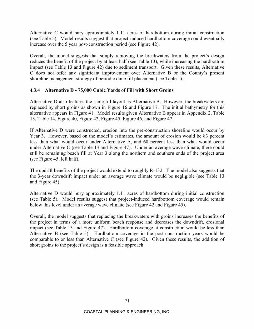
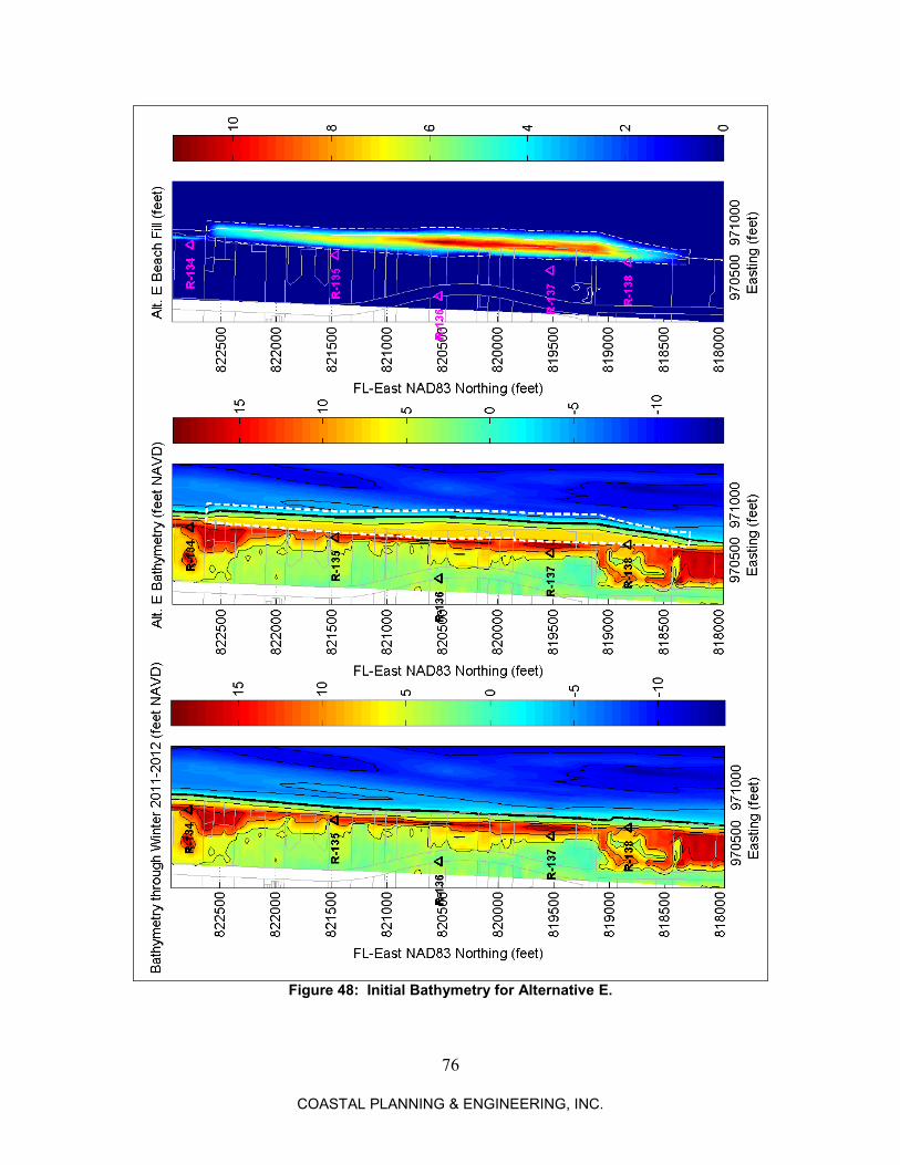
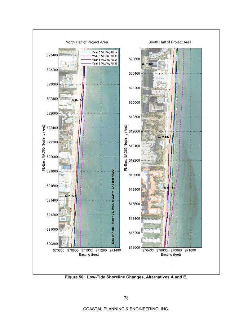
Due to the effects of recent storms and long-term erosion, the shorelines along the Towns of South Palm Beach and Lantana have been categorized as eroded. Although the long term erosional trend is moderate, erosion and shoreline retreat patterns can be highly variable due to the effects of storms, erosion waves, and nearshore hardbottom. To restore the shoreline to a moderate beach width, a shore protection project is being considered for the area between the northern end of South Palm Beach and the Ritz-Carlton hotel in Manalapan. It is anticipated that that the Palm Beach Island Beach Management Agreement (BMA) being developed in coordination with the Florida Department of Environmental Protection (FDEP) will not include an erosion control project for South Palm Beach and Lantana. Due to the extensive hardbottom, seawalls, and narrow beaches in this area, an Environmental Impact Statement (EIS) is expected to be required for projects in the area. Accordingly, Palm Beach County is now seeking a fill design without breakwaters to last 2 to 3 years. To identify the most appropriate shore protection plan, the erosion rates between 2004 and the present were reviewed to assess the present erosion patterns. Seven alternatives were then formulated based on those erosion rates and previous studies of the project area. The Delft3D morphological model was recalibrated from previous studies based on more recent erosion patterns. The performance and impact of each alternative over a 3 year project life was then assessed using the calibrated model. For comparative purposes, the no-action scenario (Alternative A) and original recommended plan (Alternative B: 13 breakwaters with 75,000 cubic yards of fill) (CPE, 2011) were simulated with the recalibrated model and compared to a fill only alternative (Alternative C: 75,000 cubic yards) and an alternative with short low-profile groins with fill (Alternative D: 7 groins with 75,000 cubic yards of fill). If Alternative B was constructed, benefits would be concentrated along the northern third of the project area and a 2,000 foot updrift segment. Benefits along the rest of the project area would be low. If Alternative C was constructed, erosion into the pre-construction beach profile over the first 3 years would likely occur. If Alternative D was constructed, the amount of erosion would be substantially less than the fill-only alternative and provide a more uniform beach due to the benefit of the groins. After 3 years, fill would still remain along the north and south ends of the project area. Based on the results of Alternative D, an erosion control solution with groins and fill was determined to be viable option and was further refined to optimize performance. Based on the initial model simulations and sediment transport analysis, several alternatives were developed using approximately 75,000 cubic yards of sand in varying fill distributions, with and without groins. In addition, a larger, fill-only alternative with 160,600 cubic yards of material was developed based on recent erosion rates to last 3 years without any structures.

ii


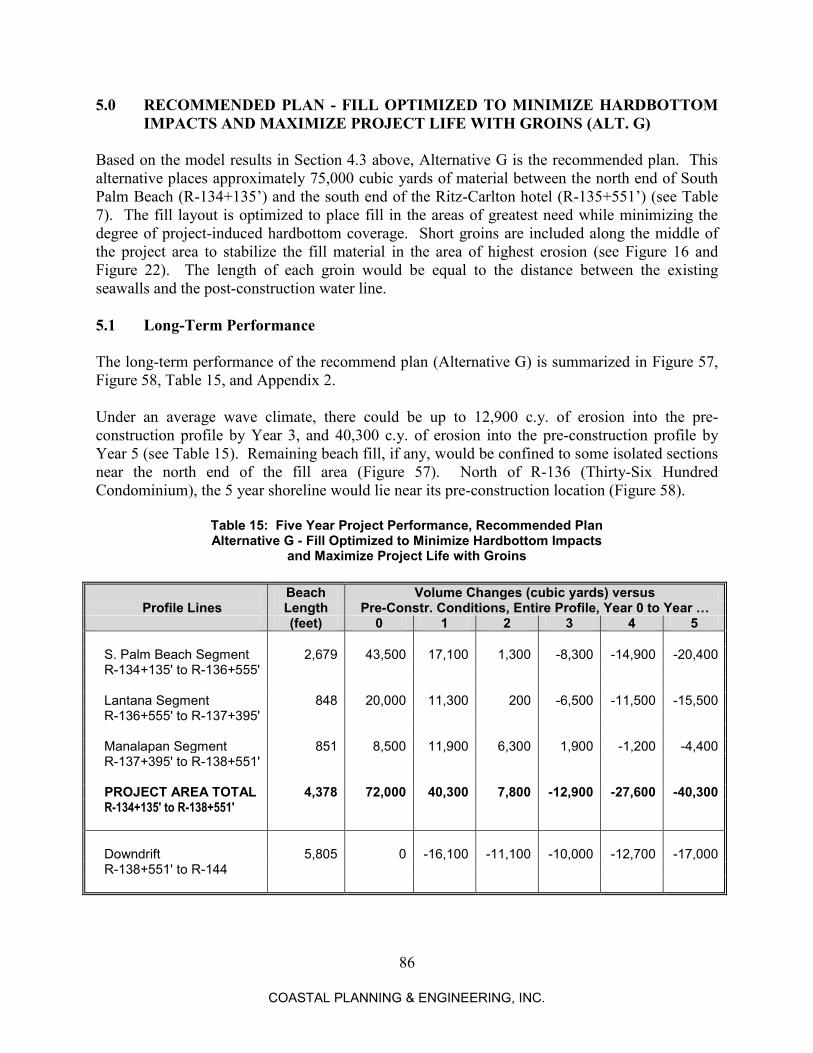
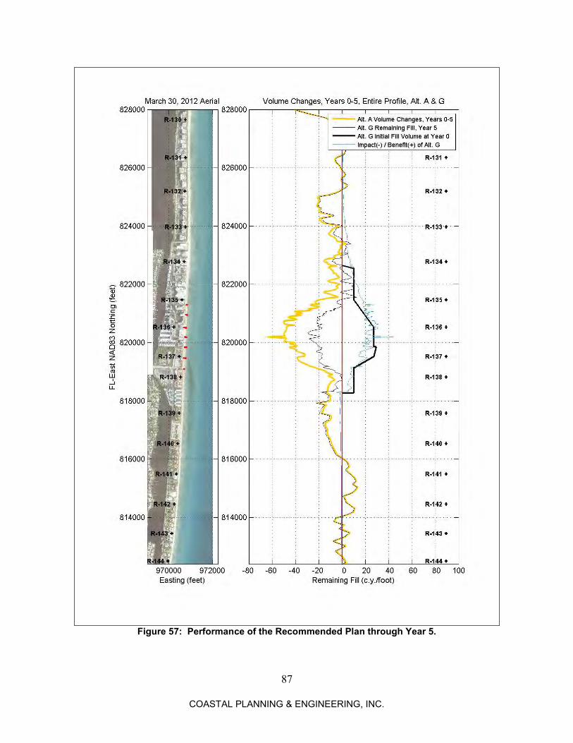
Based the results of the model simulations and analytical analyses, the County’s objective to address erosion with a moderate sized project lasting 2 to 3 years, and the improved performance of the optimized fill distribution with groin stabilization, Alternative G is the recommended plan:

Approximately 75,000 cubic yards of sand in an optimized fill distribution. Seven groins extending from the existing seawalls to the post-construction water line.

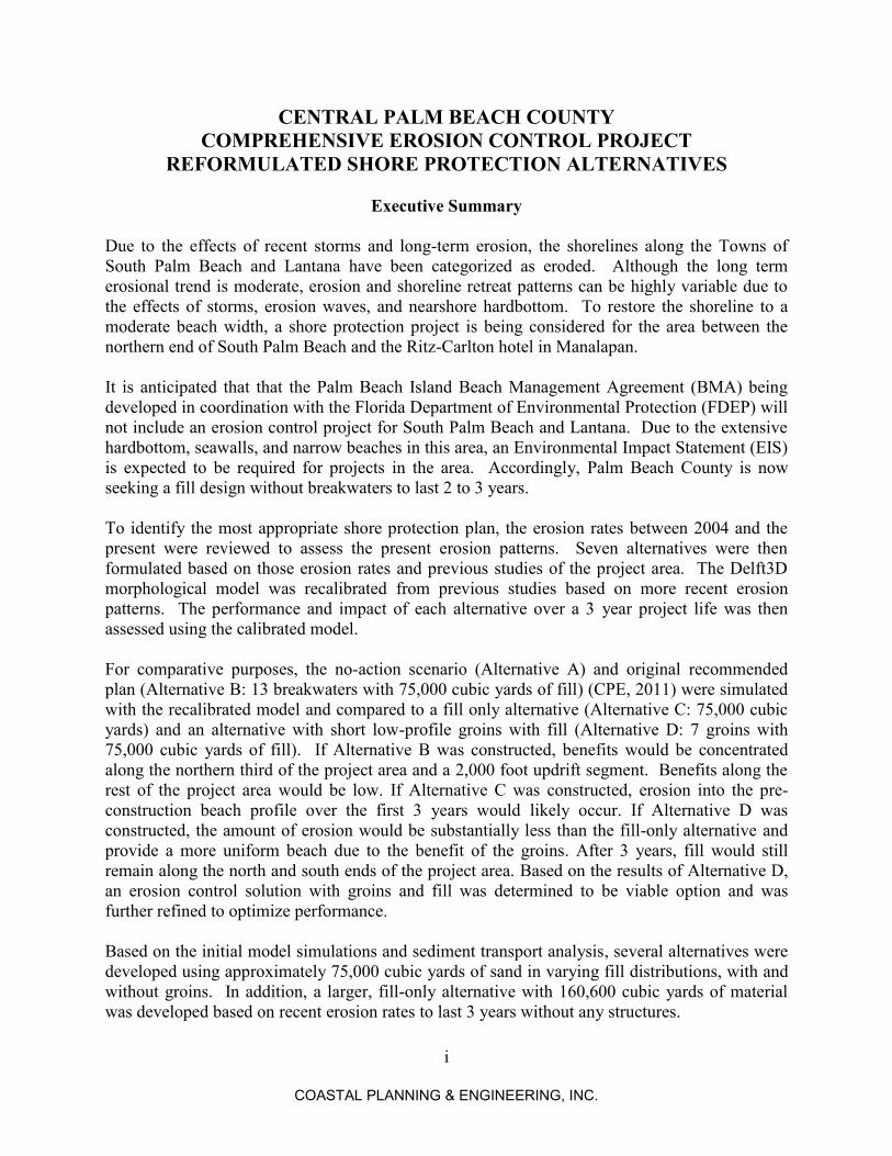
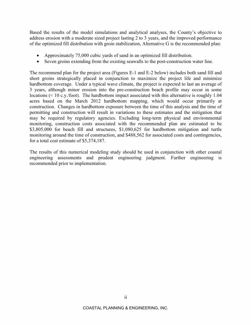
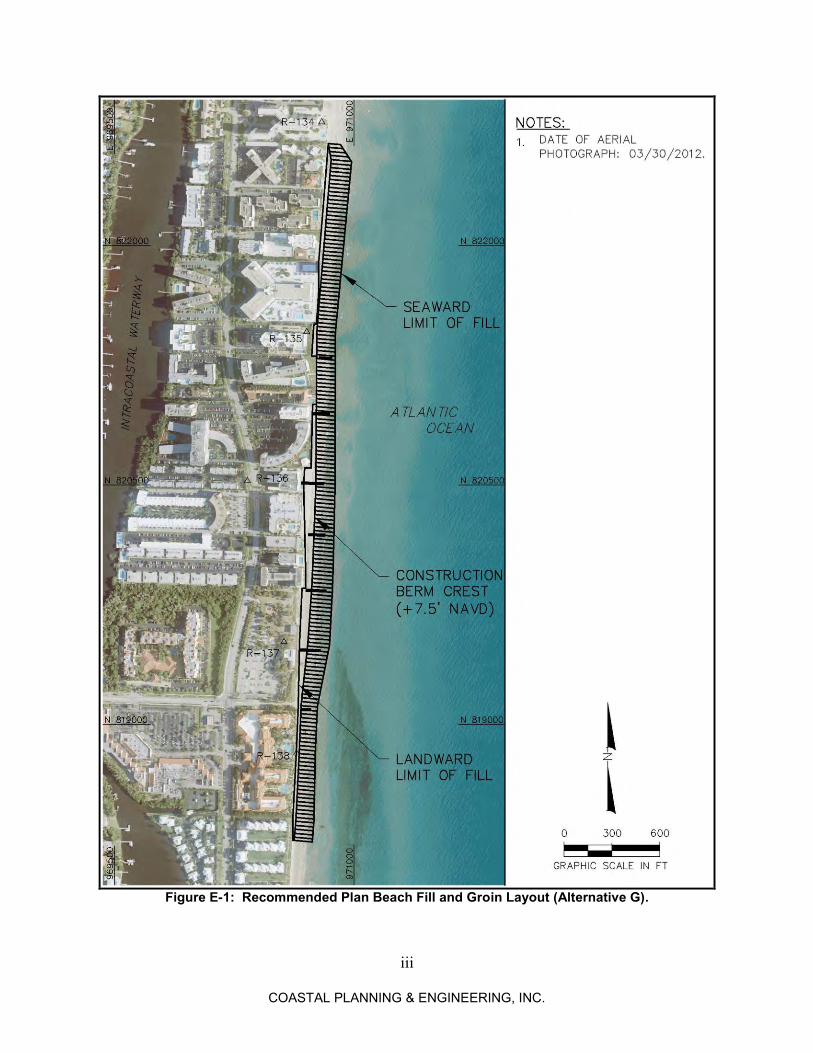
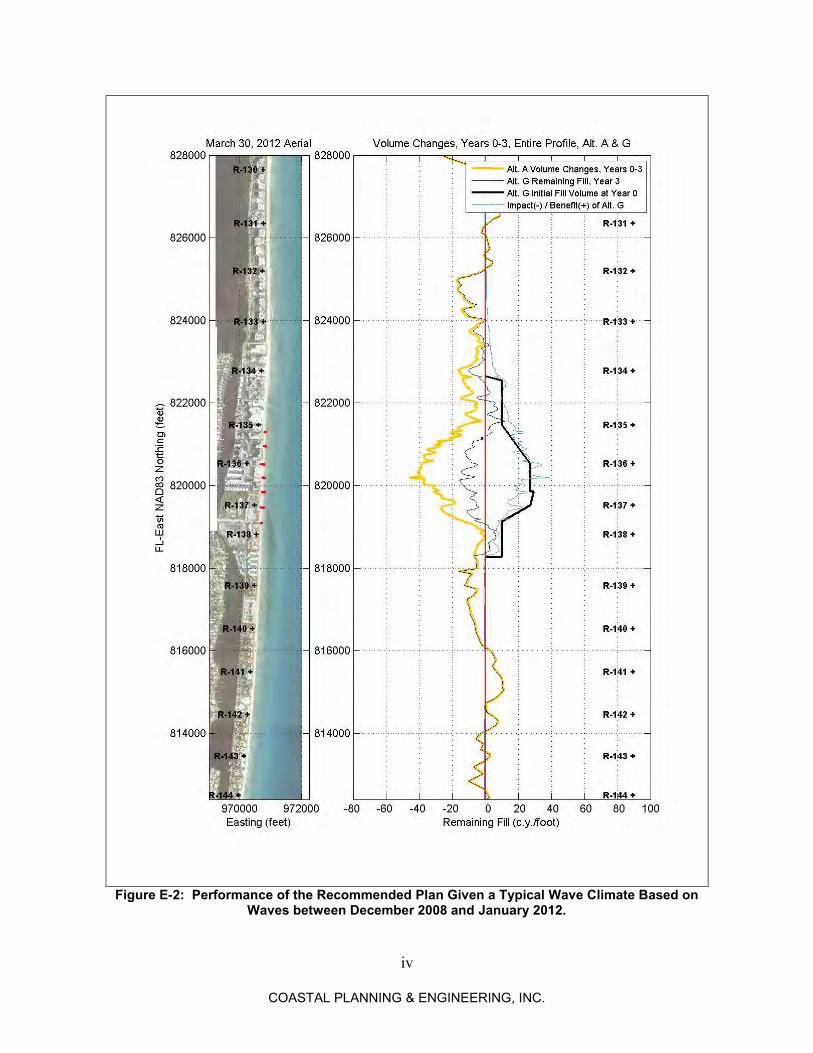
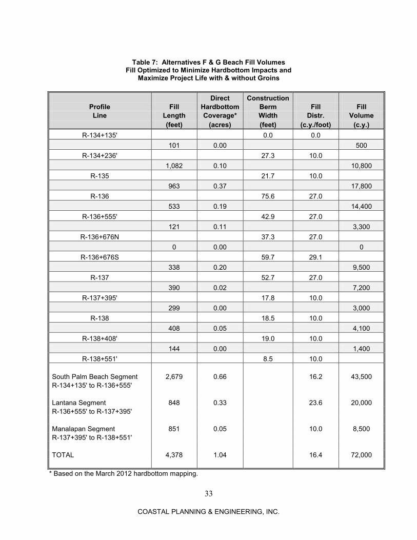
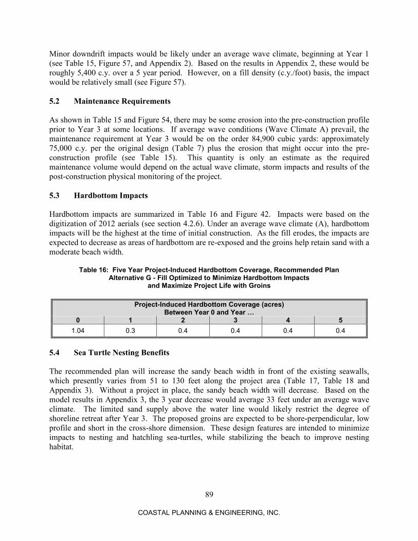
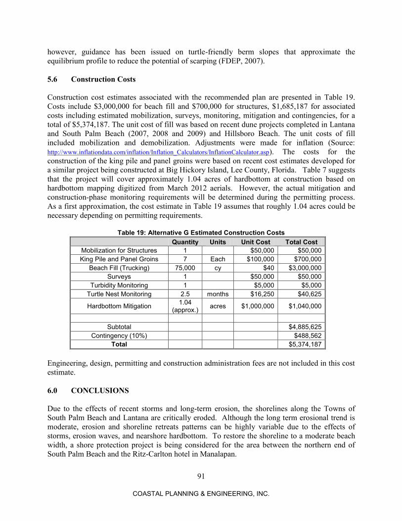
The recommend plan for the project area (Figures E-1 and E-2 below) includes both sand fill and short groins strategically placed in conjunction to maximize the project life and minimize hardbottom coverage. Under a typical wave climate, the project is expected to last an average of 3 years, although minor erosion into the pre-construction beach profile may occur in some locations (< 10 c.y./foot). The hardbottom impact associated with this alternative is roughly 1.04 acres based on the March 2012 hardbottom mapping, which would occur primarily at construction. Changes in hardbottom exposure between the time of this analysis and the time of permitting and construction will result in variations to these estimates and the mitigation that may be required by regulatory agencies. Excluding long-term physical and environmental monitoring, construction costs associated with the recommended plan are estimated to be $3,805,000 for beach fill and structures, $1,080,625 for hardbottom mitigation and turtle monitoring around the time of construction, and $488,562 for associated costs and contingencies, for a total cost estimate of $5,374,187. The results of this numerical modeling study should be used in conjunction with other coastal engineering assessments and prudent engineering judgment. Further engineering is recommended prior to implementation.

iii


Figure E-1: Recommended Plan Beach Fill and Groin Layout (Alternative G).

iv


Figure E-2: Performance of the Recommended Plan Given a Typical Wave Climate Based on

Waves between December 2008 and January 2012.

v




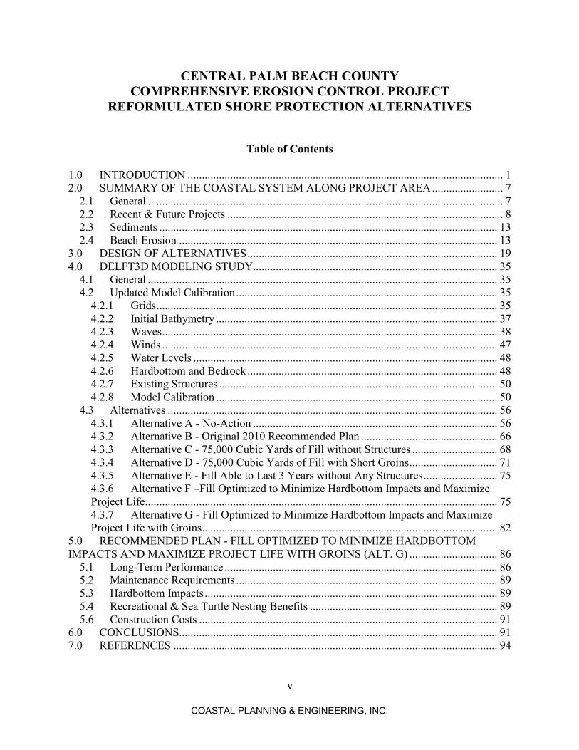
Table of Contents

1.0 INTRODUCTION ............................................................................................................... 1 2.0 SUMMARY OF THE COASTAL SYSTEM ALONG PROJECT AREA ......................... 7

2.1 General ............................................................................................................................. 7 2.2 Recent & Future Projects ................................................................................................. 8 2.3 Sediments ....................................................................................................................... 13 2.4 Beach Erosion ................................................................................................................ 13

3.0 DESIGN OF ALTERNATIVES ........................................................................................ 19 4.0 DELFT3D MODELING STUDY...................................................................................... 35

4.1 General ........................................................................................................................... 35 4.2 Updated Model Calibration ............................................................................................ 35

4.2.1 Grids ........................................................................................................................ 35 4.2.2 Initial Bathymetry ................................................................................................... 37 4.2.3 Waves ...................................................................................................................... 38 4.2.4 Winds ...................................................................................................................... 47 4.2.5 Water Levels ........................................................................................................... 48 4.2.6 Hardbottom and Bedrock ........................................................................................ 48 4.2.7 Existing Structures .................................................................................................. 50 4.2.8 Model Calibration ................................................................................................... 50

4.3 Alternatives .................................................................................................................... 56

4.3.1 Alternative A - No-Action ...................................................................................... 56 4.3.2 Alternative B - Original 2010 Recommended Plan ................................................ 66 4.3.3 Alternative C - 75,000 Cubic Yards of Fill without Structures .............................. 68 4.3.4 Alternative D - 75,000 Cubic Yards of Fill with Short Groins ............................... 71 4.3.5 Alternative E - Fill Able to Last 3 Years without Any Structures .......................... 75 4.3.6 Alternative F –Fill Optimized to Minimize Hardbottom Impacts and Maximize Project Life............................................................................................................................ 75 4.3.7 Alternative G - Fill Optimized to Minimize Hardbottom Impacts and Maximize Project Life with Groins........................................................................................................ 82

5.0 RECOMMENDED PLAN - FILL OPTIMIZED TO MINIMIZE HARDBOTTOM IMPACTS AND MAXIMIZE PROJECT LIFE WITH GROINS (ALT. G) ............................... 86

5.1 Long-Term Performance ................................................................................................ 86

5.2 Maintenance Requirements ............................................................................................ 89

5.3 Hardbottom Impacts ....................................................................................................... 89

5.4 Recreational & Sea Turtle Nesting Benefits .................................................................. 89 5.6 Construction Costs ......................................................................................................... 91

6.0 CONCLUSIONS................................................................................................................ 91 7.0 REFERENCES .................................................................................................................. 94

vi


List of Figures

Figure 1: Project Area Location. .................................................................................................... 2 Figure 2: Damaged Seawall at the Mayfair House Condominium, October 3, 2008. ................... 3 Figure 3: Damaged Sidewalk at Town of Lantana Public Beach, October 29, 2008. ................... 3 Figure 4: CPE (2011) Alternative 1. .............................................................................................. 4 Figure 5: CPE (2011) Alternative 2. .............................................................................................. 5 Figure 6: CPE (2011) Alternative 9. .............................................................................................. 6 Figure 7: Seawall under Construction at Lantana Public Beach, March 4, 2010 Photo. ............... 9 Figure 8: March 30, 2012 Aerial Photograph of Completed Lantana Public Beach Seawall. ...... 9 Figure 9: South End Palm Beach Restoration Plan View. ........................................................... 10 Figure 10: South End Palm Beach Restoration July 27, 2012 Permit Cross-Sections (Coastal Systems, 2012). ............................................................................................................................. 11 Figure 11: Recent Mean High Water (+0.45’ NAVD) Shoreline Changes. ................................ 15

Figure 12: Recent Volume Changes. ........................................................................................... 16 Figure 13: Representative Profiles at Concordia East (R-135) and Lantana Public Beach (R-137). .............................................................................................................................................. 18 Figure 14: Alternative B & C Fill Layout. ................................................................................... 21 Figure 15: Typical Breakwater Cross-Section, Alternative B (CPE, 2009). ............................... 22 Figure 16: Typical Alternative D & G Groin Cross-Section Based on CPE, 2011. .................... 24 Figure 17: Alternative D Groin & Fill Layout. ............................................................................ 25 Figure 18: Comparison of the Discrete and Analytical Solutions for a Triangular Beach Fill. .. 27 Figure 19: Predicted and Observed Performance of the 1995-96 Palm Beach Midtown Beach Nourishment Project. .................................................................................................................... 28 Figure 20: Alternative E Beach Fill Distribution and Performance Estimate Based on the Walton & Chiu (1979) Analytical Method. ............................................................................................... 29 Figure 21: Alternative E Fill Layout. ........................................................................................... 30

Figure 22: Alternatives F & G Fill & Groin Layout. ................................................................... 34 Figure 23: Computational Grids for the SWAN and Delft3D-FLOW Models. .......................... 36 Figure 24: Regional Wave Grid Bathymetry. .............................................................................. 39 Figure 25: Intermediate Wave Grid Bathymetry. ........................................................................ 40 Figure 26: Initial, 2008 Bathymetry over the Local Wave Grid & the Flow & Morphology Grid........................................................................................................................................................ 41 Figure 27: Offshore Directional Wave Statistics from 1999 to 2008 .......................................... 42 Figure 28: Monthly Offshore Wave Statistics. ............................................................................ 43 Figure 29: Monthly Variation of Wave Direction Offshore. ....................................................... 44

Figure 30: Wave Rose Showing Dec. 2008 to Jan. 2012 Wave Cases (numbers) and Wave Records (light-colored dots). ........................................................................................................ 47

Figure 31: January 24, 2009 Aerial Photograph of the Lake Worth Pier. ................................... 52 Figure 32: Typical Survey Profiles (R-133) across the Phipps Ocean Park South Borrow Area.52

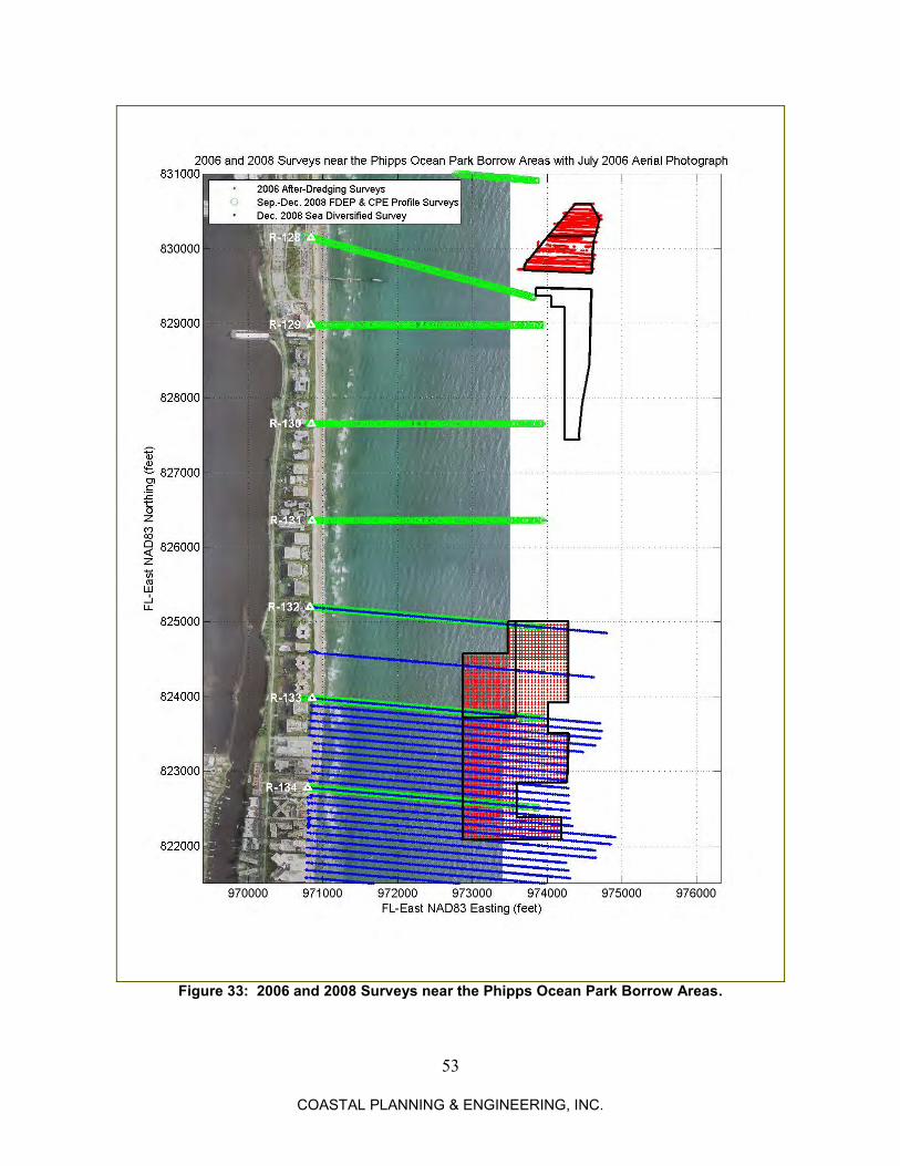
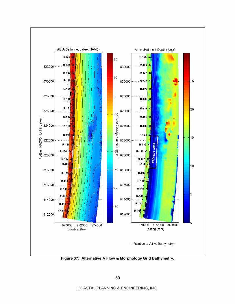
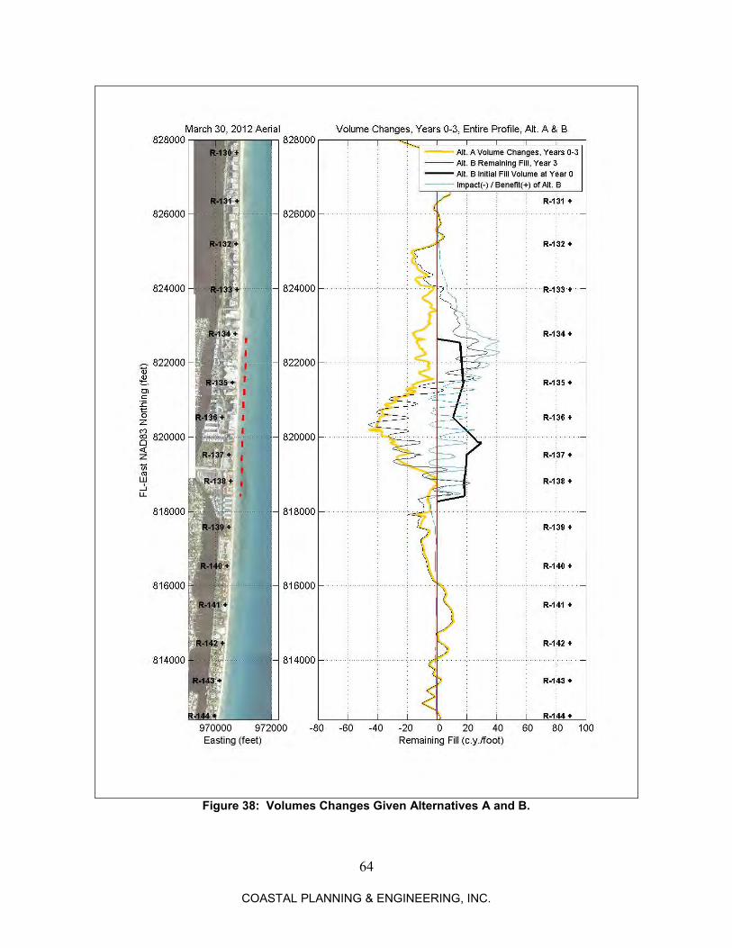
Figure 33: 2006 and 2008 Surveys near the Phipps Ocean Park Borrow Areas.......................... 53 Figure 34: Hardbottom/Bedrock Elevations Used in the Final Calibration Run. ........................ 55 Figure 35: Simulated Volume Changes during the Final Calibration Run. ................................. 57 Figure 36: 2011-2012 and Alternative A Bathymetry Comparison............................................. 59 Figure 37: Alternative A Flow & Morphology Grid Bathymetry................................................ 60 Figure 38: Volumes Changes Given Alternatives A and B. ........................................................ 64

vii


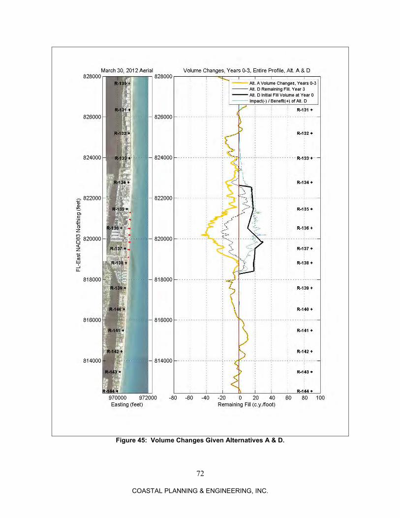
Figure 39: Low-Tide Shoreline Changes, Alternatives A and B. ................................................ 65

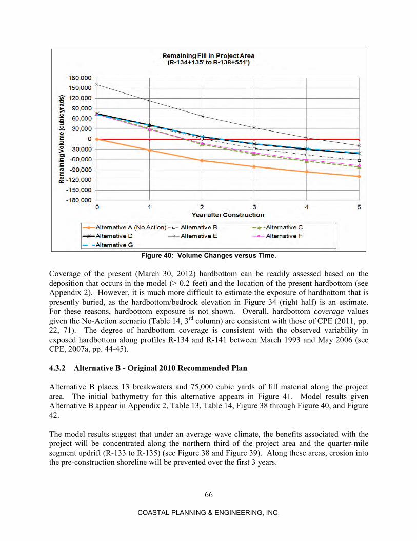
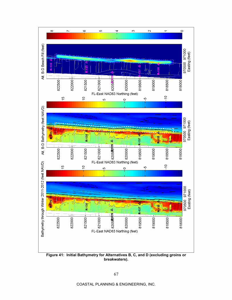
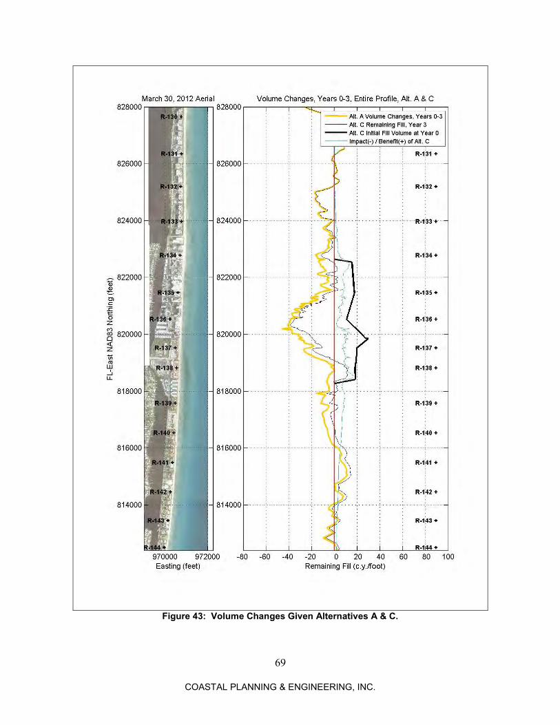
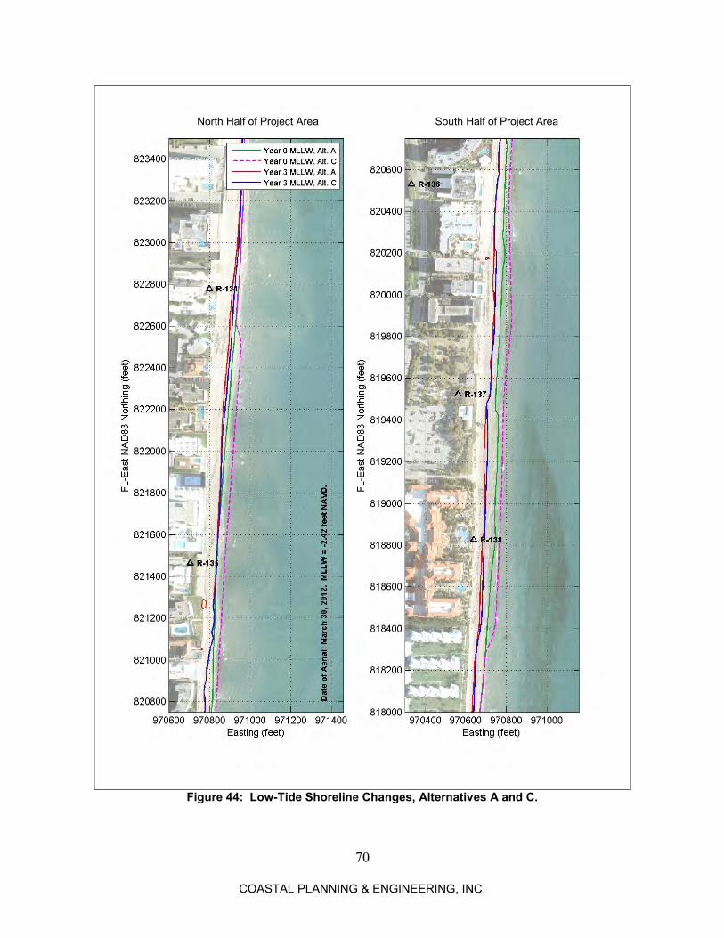
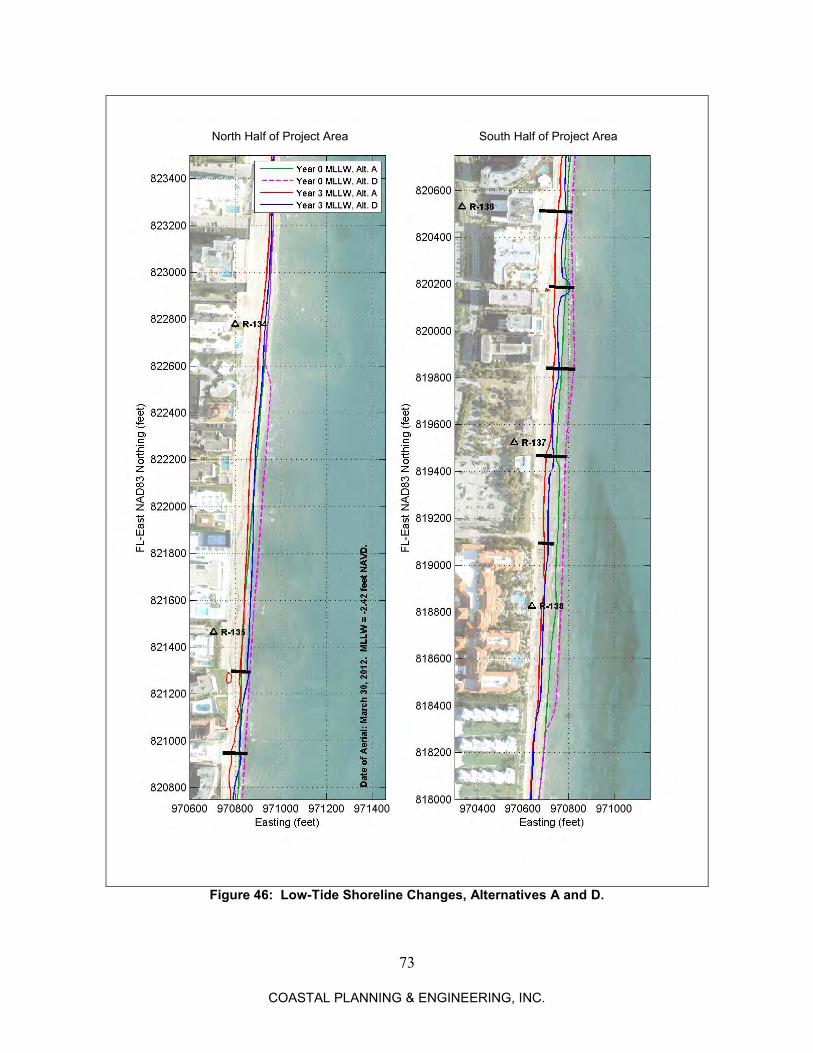
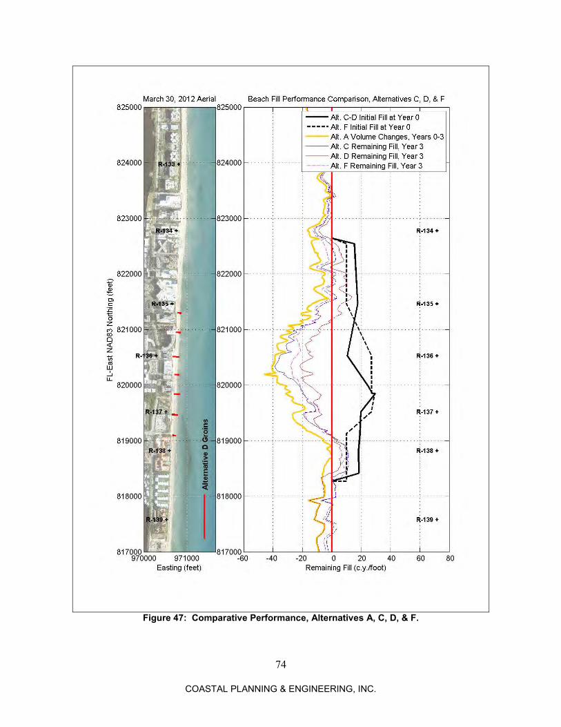
Figure 40: Volume Changes versus Time. ................................................................................... 66 Figure 41: Initial Bathymetry for Alternatives B, C, and D (excluding groins or breakwaters). 67 Figure 42: Project-Induced Hardbottom Coverage versus Time. ................................................ 68 Figure 43: Volume Changes Given Alternatives A & C. ............................................................ 69 Figure 44: Low-Tide Shoreline Changes, Alternatives A and C. ................................................ 70 Figure 45: Volume Changes Given Alternatives A & D. ............................................................ 72 Figure 46: Low-Tide Shoreline Changes, Alternatives A and D. ................................................ 73 Figure 47: Comparative Performance, Alternatives A, C, D, & F. .............................................. 74 Figure 48: Initial Bathymetry for Alternative E. ......................................................................... 76 Figure 49: Volume Changes Given Alternatives A & E.............................................................. 77 Figure 50: Low-Tide Shoreline Changes, Alternatives A and E. ................................................ 78 Figure 51: Initial Bathymetry for Alternatives F & G (excluding groins). .................................. 79 Figure 52: Volume Changes Given Alternatives A & F. ............................................................. 80

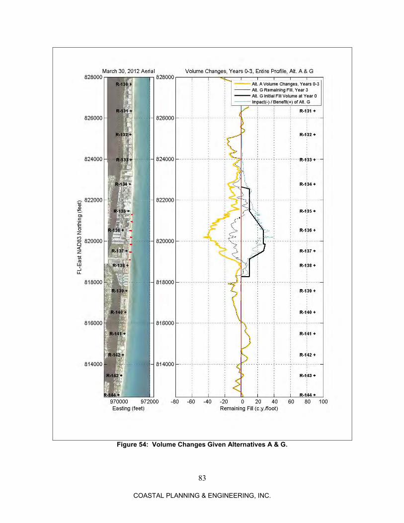
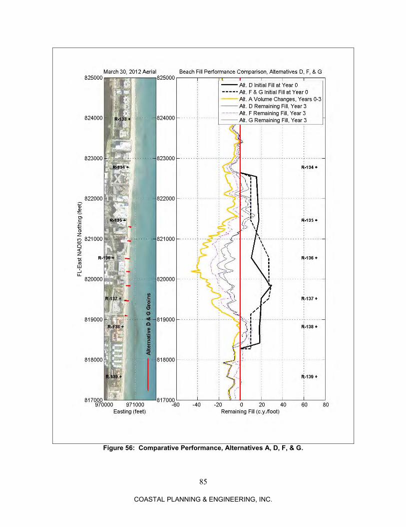
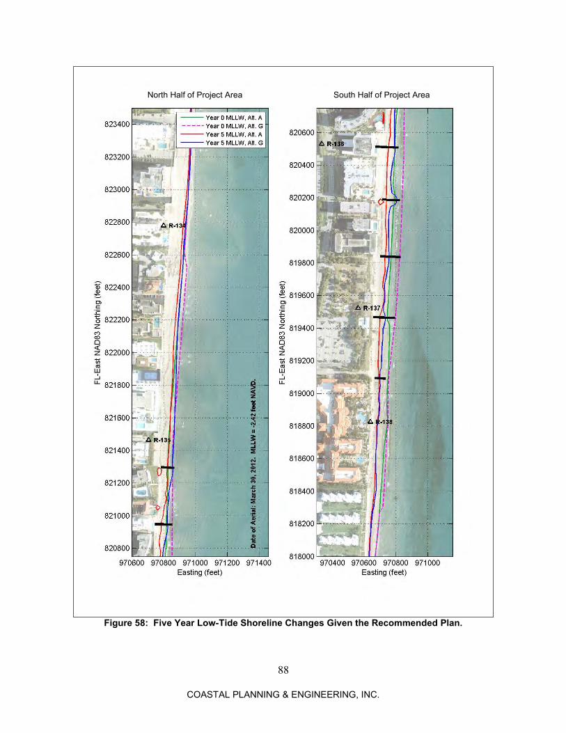
Figure 53: Low-Tide Shoreline Changes, Alternatives A and F. ................................................ 81 Figure 54: Volume Changes Given Alternatives A & G. ............................................................ 83 Figure 55: Low-Tide Shoreline Changes, Alternatives A and G. ................................................ 84 Figure 56: Comparative Performance, Alternatives A, D, F, & G. ............................................. 85 Figure 57: Performance of the Recommended Plan through Year 5. .......................................... 87 Figure 58: Five Year Low-Tide Shoreline Changes Given the Recommended Plan. ................. 88

List of Tables Table 1: South Palm Beach & Lantana Dune Projects .................................................................. 8 Table 2: 2010-2011 Dune Restoration Bid Volumes, Town of Palm Beach (ATM, 2009) ........ 12 Table 3: Bathymetric & Topographic Data Sources .................................................................... 14 Table 4: September-December 2008 to January 2012 Volume Change Rates ............................ 17

Table 5: Alternative B-D Beach Fill Volumes ............................................................................ 20 Table 6: Alternative E Beach Fill Volumes ................................................................................. 31 Table 7: Alternatives F & G Beach Fill Volumes........................................................................ 33 Table 8: Computational Grid Characteristics .............................................................................. 37 Table 9: Dec. 2008 to Jan. 2012 Wave Climate A....................................................................... 46 Table 10: Tidal Datums, Lake Worth Pier (NOAA, 2003).......................................................... 48

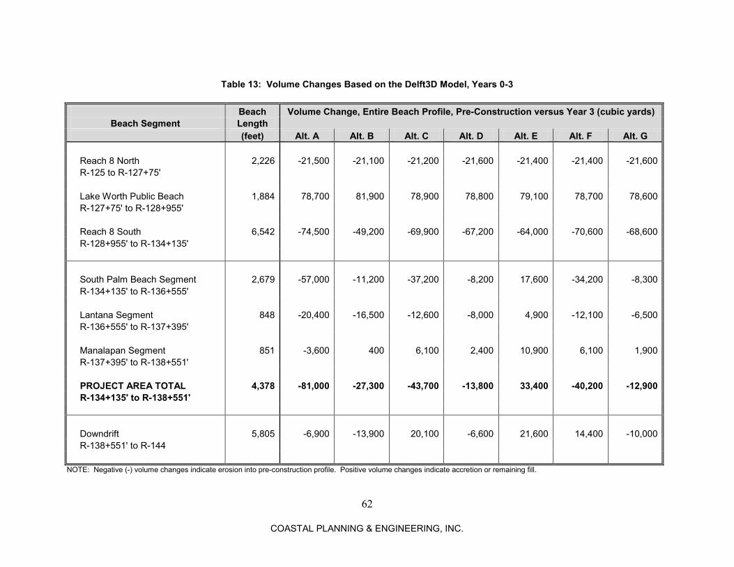
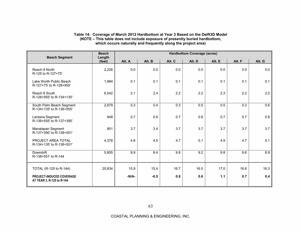
Table 11: Surveys Used to Estimate Hardbottom Outcropping Elevations in Feet NAVD. ....... 49 Table 12: Delft3D Calibration Parameters, South Palm Beach, FL ............................................ 58 Table 13: Volume Changes Based on the Delft3D Model, Years 0-3 ......................................... 62 Table 14: Coverage of March 2012 Hardbottom at Year 3 Based on the Delft3D Model .......... 63 Table 15: Five Year Project Performance, Recommended Plan .................................................. 86

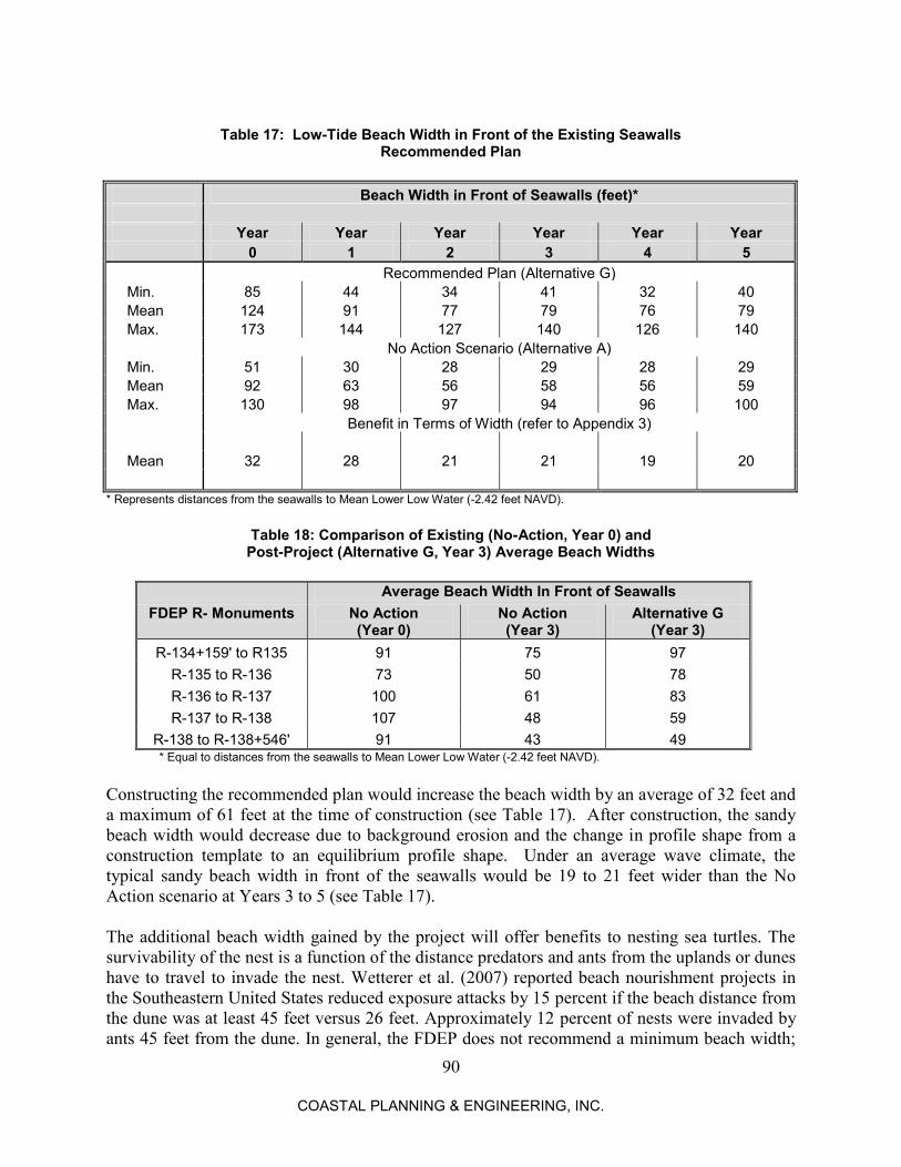
Table 16: Five Year Project-Induced Hardbottom Coverage, Recommended Plan .................... 89 Table 17: Low-Tide Beach Width in Front of the Existing Seawalls .......................................... 90

Table 18: Comparison of Existing (No-Action, Year 0) and Post-Project (Alternative G, Year 3) Average Beach Widths ................................................................................................................. 90 Table 19: Alternative G Estimated Construction Costs ................................................................ 91

viii


List of Appendices Appendix No. 1 Beach Profiles Used to Estimate Observed Erosion Rates 2 Delft3D Model Results Assuming

December 2008 to January 2012 Waves

3 Dry Beach Width in Front of the Existing Seawalls Given the Recommended Plan

1



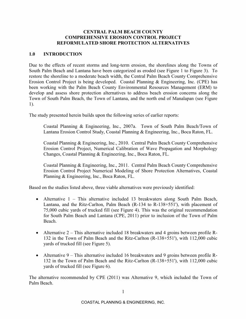
REFORMULATED SHORE PROTECTION ALTERNATIVES 1.0 INTRODUCTION Due to the effects of recent storms and long-term erosion, the shorelines along the Towns of South Palm Beach and Lantana have been categorized as eroded (see Figure 1 to Figure 3). To restore the shoreline to a moderate beach width, the Central Palm Beach County Comprehensive Erosion Control Project is being developed. Coastal Planning & Engineering, Inc. (CPE) has been working with the Palm Beach County Environmental Resources Management (ERM) to develop and assess shore protection alternatives to address beach erosion concerns along the Town of South Palm Beach, the Town of Lantana, and the north end of Manalapan (see Figure 1). The study presented herein builds upon the following series of earlier reports:

Coastal Planning & Engineering, Inc., 2007a. Town of South Palm Beach/Town of Lantana Erosion Control Study, Coastal Planning & Engineering, Inc., Boca Raton, FL. Coastal Planning & Engineering, Inc., 2010. Central Palm Beach County Comprehensive Erosion Control Project, Numerical Calibration of Wave Propagation and Morphology Changes, Coastal Planning & Engineering, Inc., Boca Raton, FL. Coastal Planning & Engineering, Inc., 2011. Central Palm Beach County Comprehensive Erosion Control Project Numerical Modeling of Shore Protection Alternatives, Coastal Planning & Engineering, Inc., Boca Raton, FL.

Based on the studies listed above, three viable alternatives were previously identified:

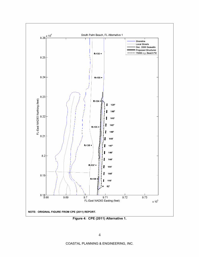
Alternative 1 – This alternative included 13 breakwaters along South Palm Beach, Lantana, and the Ritz-Carlton, Palm Beach (R-134 to R-138+551'), with placement of 75,000 cubic yards of trucked fill (see Figure 4). This was the original recommendation for South Palm Beach and Lantana (CPE, 2011) prior to inclusion of the Town of Palm Beach.

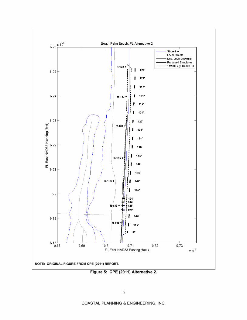
Alternative 2 – This alternative included 18 breakwaters and 4 groins between profile R-132 in the Town of Palm Beach and the Ritz-Carlton (R-138+551'), with 112,000 cubic yards of trucked fill (see Figure 5).

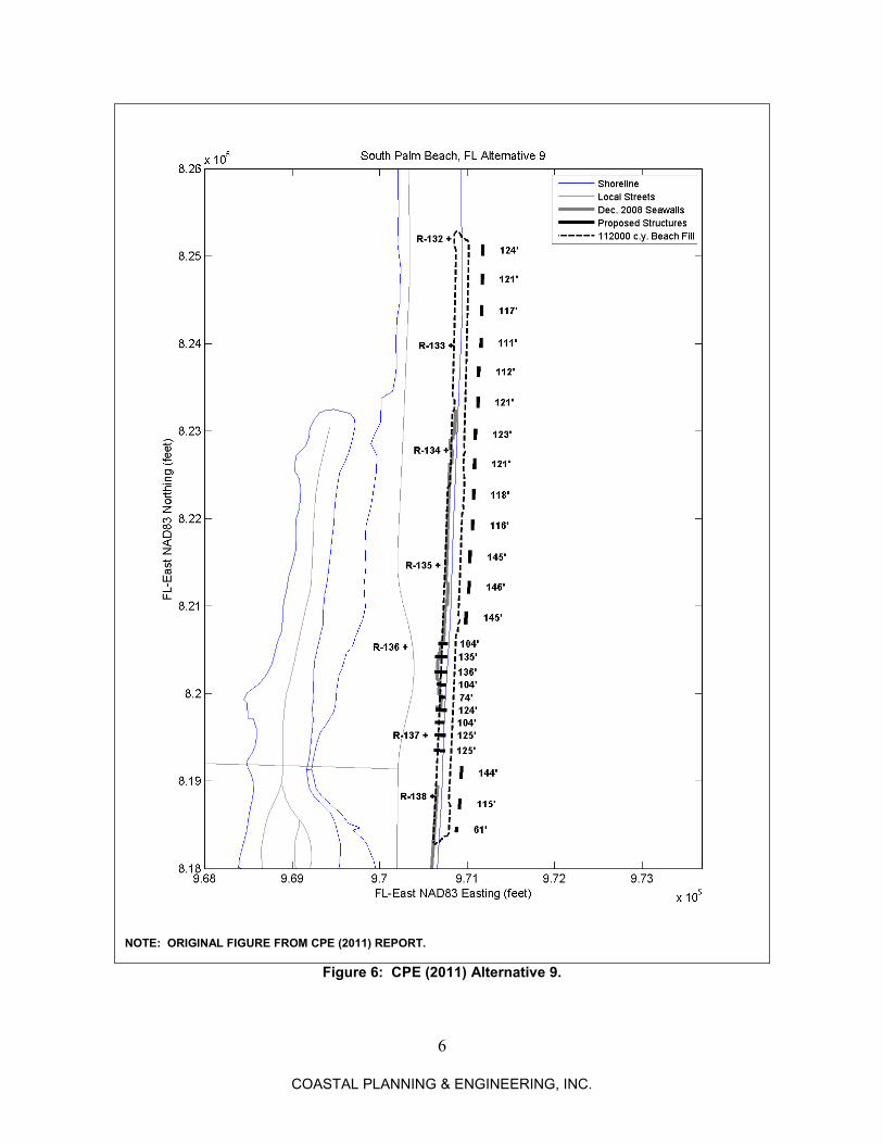
Alternative 9 – This alternative included 16 breakwaters and 9 groins between profile R-132 in the Town of Palm Beach and the Ritz-Carlton (R-138+551'), with 112,000 cubic yards of trucked fill (see Figure 6).

The alternative recommended by CPE (2011) was Alternative 9, which included the Town of Palm Beach.

2


Figure 1: Project Area Location.

City

of L

ake

Wor

th

Town of Palm Beach

Town of Lantana

Town of South Palm Beach

Town of Manalapan

PRO

JEC

T A

REA

3


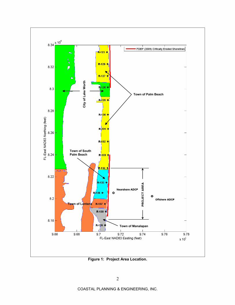
Figure 2: Damaged Seawall at the Mayfair House Condominium, October 3, 2008.

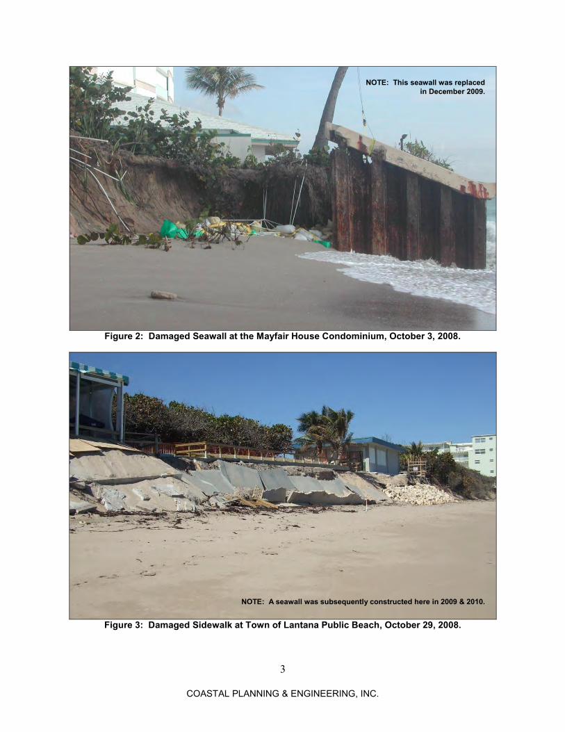
Figure 3: Damaged Sidewalk at Town of Lantana Public Beach, October 29, 2008.

NOTE: This seawall was replaced in December 2009.

NOTE: A seawall was subsequently constructed here in 2009 & 2010.

4


Figure 4: CPE (2011) Alternative 1.

NOTE: ORIGINAL FIGURE FROM CPE (2011) REPORT.

5




6




7


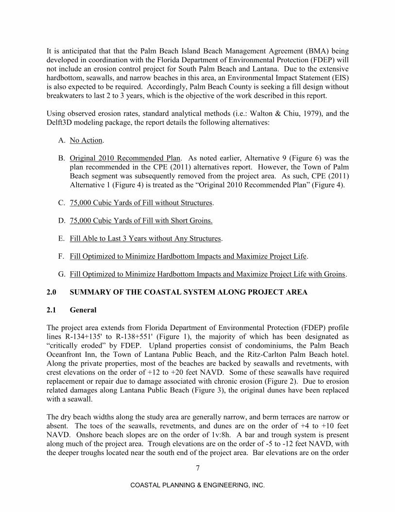
It is anticipated that that the Palm Beach Island Beach Management Agreement (BMA) being developed in coordination with the Florida Department of Environmental Protection (FDEP) will not include an erosion control project for South Palm Beach and Lantana. Due to the extensive hardbottom, seawalls, and narrow beaches in this area, an Environmental Impact Statement (EIS) is also expected to be required. Accordingly, Palm Beach County is seeking a fill design without breakwaters to last 2 to 3 years, which is the objective of the work described in this report. Using observed erosion rates, standard analytical methods (i.e.: Walton & Chiu, 1979), and the Delft3D modeling package, the report details the following alternatives:

A. No Action.

B. Original 2010 Recommended Plan. As noted earlier, Alternative 9 (Figure 6) was the plan recommended in the CPE (2011) alternatives report. However, the Town of Palm Beach segment was subsequently removed from the project area. As such, CPE (2011) Alternative 1 (Figure 4) is treated as the “Original 2010 Recommended Plan” (Figure 4).

C. 75,000 Cubic Yards of Fill without Structures.

D. 75,000 Cubic Yards of Fill with Short Groins.

E. Fill Able to Last 3 Years without Any Structures.

F. Fill Optimized to Minimize Hardbottom Impacts and Maximize Project Life.

G. Fill Optimized to Minimize Hardbottom Impacts and Maximize Project Life with Groins. 2.0 SUMMARY OF THE COASTAL SYSTEM ALONG PROJECT AREA 2.1 General The project area extends from Florida Department of Environmental Protection (FDEP) profile lines R-134+135' to R-138+551' (Figure 1), the majority of which has been designated as “critically eroded” by FDEP. Upland properties consist of condominiums, the Palm Beach Oceanfront Inn, the Town of Lantana Public Beach, and the Ritz-Carlton Palm Beach hotel. Along the private properties, most of the beaches are backed by seawalls and revetments, with crest elevations on the order of +12 to +20 feet NAVD. Some of these seawalls have required replacement or repair due to damage associated with chronic erosion (Figure 2). Due to erosion related damages along Lantana Public Beach (Figure 3), the original dunes have been replaced with a seawall. The dry beach widths along the study area are generally narrow, and berm terraces are narrow or absent. The toes of the seawalls, revetments, and dunes are on the order of +4 to +10 feet NAVD. Onshore beach slopes are on the order of 1v:8h. A bar and trough system is present along much of the project area. Trough elevations are on the order of -5 to -12 feet NAVD, with the deeper troughs located near the south end of the project area. Bar elevations are on the order

8


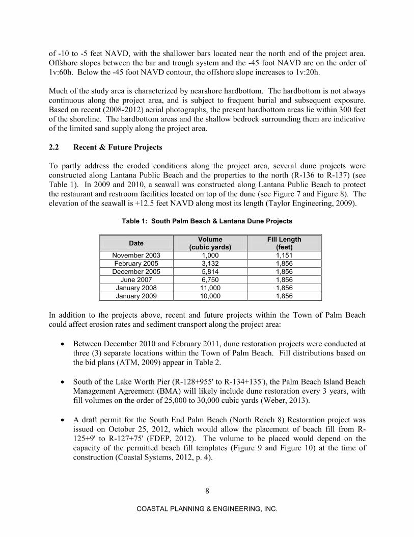
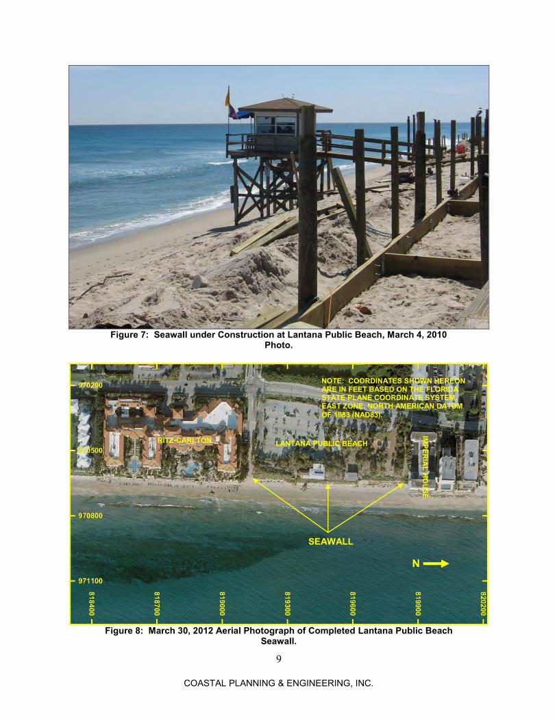
of -10 to -5 feet NAVD, with the shallower bars located near the north end of the project area. Offshore slopes between the bar and trough system and the -45 foot NAVD are on the order of 1v:60h. Below the -45 foot NAVD contour, the offshore slope increases to 1v:20h. Much of the study area is characterized by nearshore hardbottom. The hardbottom is not always continuous along the project area, and is subject to frequent burial and subsequent exposure. Based on recent (2008-2012) aerial photographs, the present hardbottom areas lie within 300 feet of the shoreline. The hardbottom areas and the shallow bedrock surrounding them are indicative of the limited sand supply along the project area. 2.2 Recent & Future Projects To partly address the eroded conditions along the project area, several dune projects were constructed along Lantana Public Beach and the properties to the north (R-136 to R-137) (see Table 1). In 2009 and 2010, a seawall was constructed along Lantana Public Beach to protect the restaurant and restroom facilities located on top of the dune (see Figure 7 and Figure 8). The elevation of the seawall is +12.5 feet NAVD along most its length (Taylor Engineering, 2009).

Table 1: South Palm Beach & Lantana Dune Projects

Date Volume (cubic yards)

Fill Length (feet)

November 2003 1,000 1,151 February 2005 3,132 1,856

December 2005 5,814 1,856 June 2007 6,750 1,856

January 2008 11,000 1,856 January 2009 10,000 1,856

In addition to the projects above, recent and future projects within the Town of Palm Beach could affect erosion rates and sediment transport along the project area:

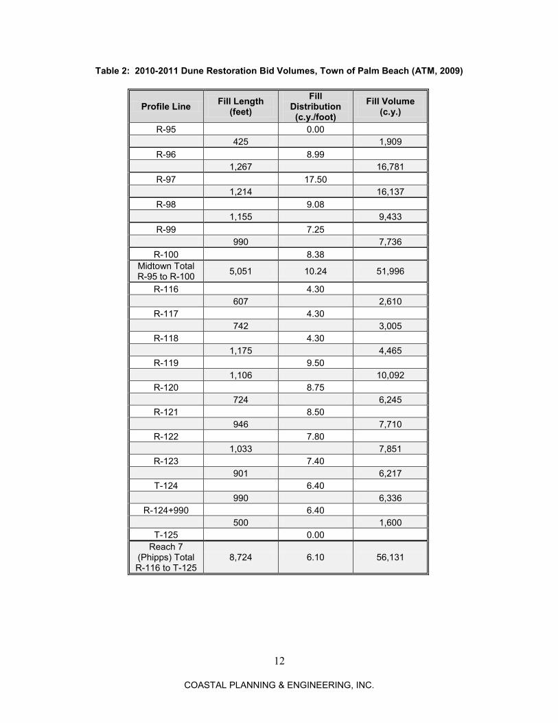
Between December 2010 and February 2011, dune restoration projects were conducted at three (3) separate locations within the Town of Palm Beach. Fill distributions based on the bid plans (ATM, 2009) appear in Table 2.

South of the Lake Worth Pier (R-128+955' to R-134+135'), the Palm Beach Island Beach Management Agreement (BMA) will likely include dune restoration every 3 years, with fill volumes on the order of 25,000 to 30,000 cubic yards (Weber, 2013).

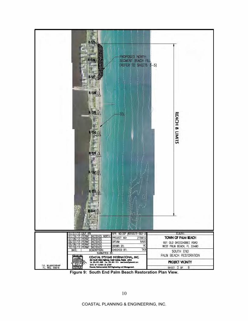
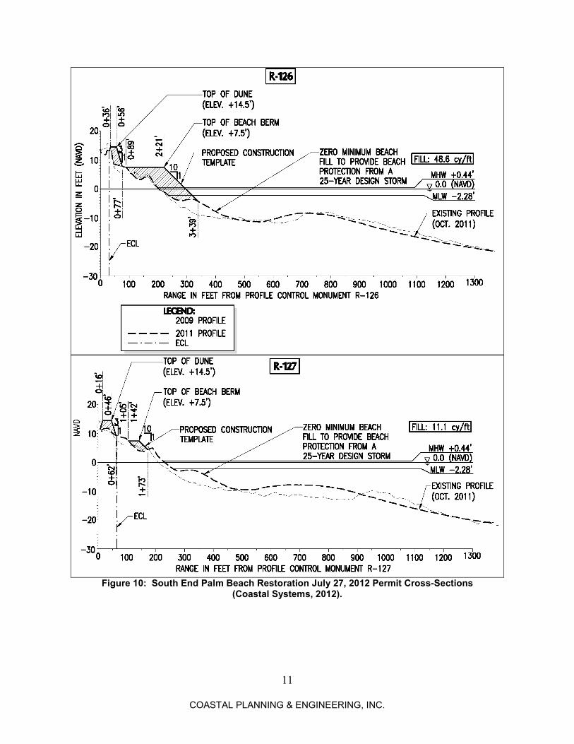
A draft permit for the South End Palm Beach (North Reach 8) Restoration project was issued on October 25, 2012, which would allow the placement of beach fill from R-125+9' to R-127+75' (FDEP, 2012). The volume to be placed would depend on the capacity of the permitted beach fill templates (Figure 9 and Figure 10) at the time of construction (Coastal Systems, 2012, p. 4).

9


Figure 7: Seawall under Construction at Lantana Public Beach, March 4, 2010

Photo.

Figure 8: March 30, 2012 Aerial Photograph of Completed Lantana Public Beach

Seawall.

NOTE: COORDINATES SHOWN HEREON ARE IN FEET BASED ON THE FLORIDA STATE PLANE COORDINATE SYSTEM, EAST ZONE, NORTH AMERICAN DATUM OF 1983 (NAD83).

N

RITZ-CARLTON LANTANA PUBLIC BEACH

IMPER

IAL H

OU

SE

SEAWALL

10


Figure 9: South End Palm Beach Restoration Plan View.

11


Figure 10: South End Palm Beach Restoration July 27, 2012 Permit Cross-Sections

(Coastal Systems, 2012).

12


Table 2: 2010-2011 Dune Restoration Bid Volumes, Town of Palm Beach (ATM, 2009)

Profile Line Fill Length (feet)

Fill Distribution (c.y./foot)

Fill Volume (c.y.)

R-95

0.00 425 1,909

R-96 8.99 1,267 16,781

R-97 17.50 1,214 16,137

R-98 9.08 1,155 9,433

R-99 7.25 990 7,736

R-100 8.38 Midtown Total R-95 to R-100 5,051 10.24 51,996

R-116

4.30 607 2,610

R-117

4.30 742 3,005

R-118

4.30 1,175 4,465

R-119

9.50 1,106 10,092

R-120

8.75 724 6,245

R-121

8.50 946 7,710

R-122

7.80 1,033 7,851

R-123

7.40 901 6,217

T-124

6.40 990 6,336

R-124+990

6.40 500 1,600

T-125

0.00 Reach 7

(Phipps) Total R-116 to T-125

8,724 6.10 56,131

13


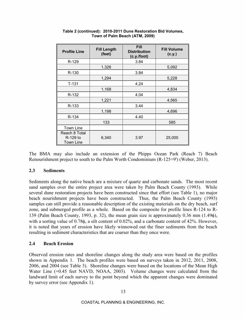
Table 2 (continued): 2010-2011 Dune Restoration Bid Volumes, Town of Palm Beach (ATM, 2009)

Profile Line Fill Length (feet)

Fill Distribution (c.y./foot)

Fill Volume (c.y.)

R-129

3.84 1,326 5,092

R-130 3.84 1,294 5,228

T-131 4.24 1,168 4,834

R-132 4.04 1,221 4,565

R-133 3.44 1,198 4,696

R-134 4.40 133 585

Town Line 4.40 Reach 8 Total

R-129 to Town Line

6,340 3.97 25,000

The BMA may also include an extension of the Phipps Ocean Park (Reach 7) Beach Renourishment project to south to the Palm Worth Condominium (R-125+9') (Weber, 2013). 2.3 Sediments Sediments along the native beach are a mixture of quartz and carbonate sands. The most recent sand samples over the entire project area were taken by Palm Beach County (1993). While several dune restoration projects have been constructed since that effort (see Table 1), no major beach nourishment projects have been constructed. Thus, the Palm Beach County (1993) samples can still provide a reasonable description of the existing materials on the dry beach, surf zone, and submerged profile as a whole. Based on the composite for profile lines R-124 to R-139 (Palm Beach County, 1993, p. 32), the mean grain size is approximately 0.36 mm (1.49), with a sorting value of 0.78, a silt content of 0.02%, and a carbonate content of 42%. However, it is noted that years of erosion have likely winnowed out the finer sediments from the beach resulting in sediment characteristics that are coarser than they once were. 2.4 Beach Erosion Observed erosion rates and shoreline changes along the study area were based on the profiles shown in Appendix 1. The beach profiles were based on surveys taken in 2012, 2011, 2008, 2006, and 2004 (see Table 3). Shoreline changes were based on the locations of the Mean High Water Line (+0.45 feet NAVD, NOAA, 2003). Volume changes were calculated from the landward limit of each survey to the point beyond which the apparent changes were dominated by survey error (see Appendix 1).

14


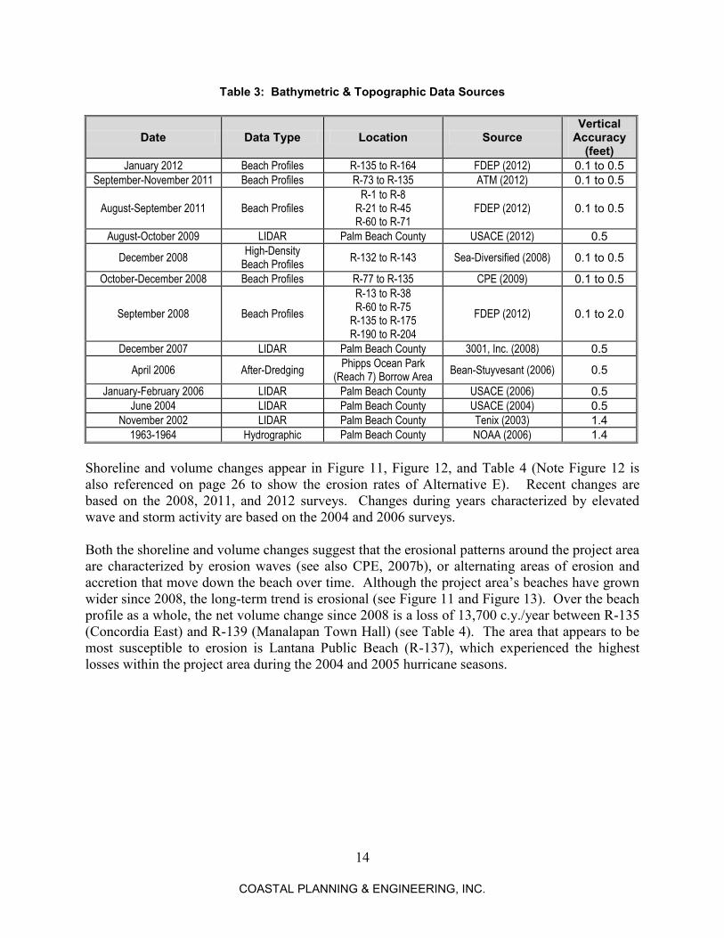
Table 3: Bathymetric & Topographic Data Sources

Date Data Type Location Source Vertical

Accuracy (feet)

January 2012 Beach Profiles R-135 to R-164 FDEP (2012) 0.1 to 0.5 September-November 2011 Beach Profiles R-73 to R-135 ATM (2012) 0.1 to 0.5

August-September 2011 Beach Profiles R-1 to R-8

R-21 to R-45 R-60 to R-71

FDEP (2012) 0.1 to 0.5

August-October 2009 LIDAR Palm Beach County USACE (2012) 0.5

December 2008 High-Density

Beach Profiles R-132 to R-143 Sea-Diversified (2008) 0.1 to 0.5

October-December 2008 Beach Profiles R-77 to R-135 CPE (2009) 0.1 to 0.5

September 2008 Beach Profiles

R-13 to R-38 R-60 to R-75

R-135 to R-175 R-190 to R-204

FDEP (2012) 0.1 to 2.0

December 2007 LIDAR Palm Beach County 3001, Inc. (2008) 0.5

April 2006 After-Dredging Phipps Ocean Park

(Reach 7) Borrow Area Bean-Stuyvesant (2006) 0.5

January-February 2006 LIDAR Palm Beach County USACE (2006) 0.5 June 2004 LIDAR Palm Beach County USACE (2004) 0.5

November 2002 LIDAR Palm Beach County Tenix (2003) 1.4 1963-1964 Hydrographic Palm Beach County NOAA (2006) 1.4

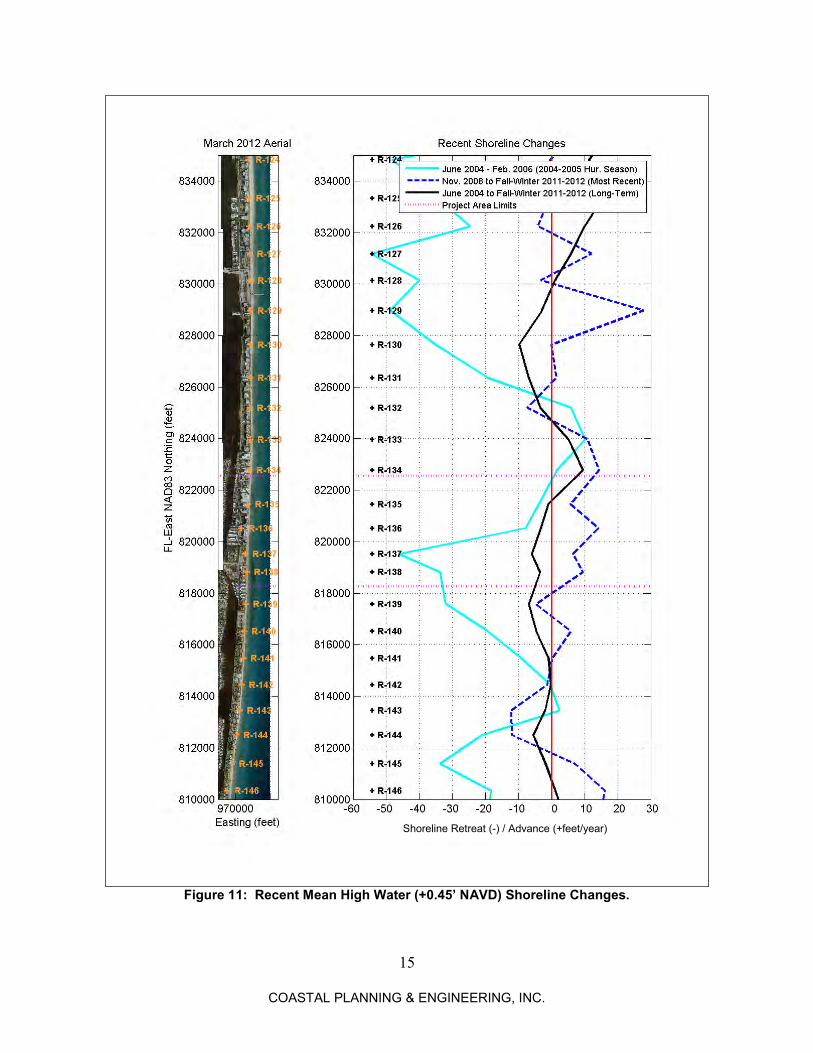
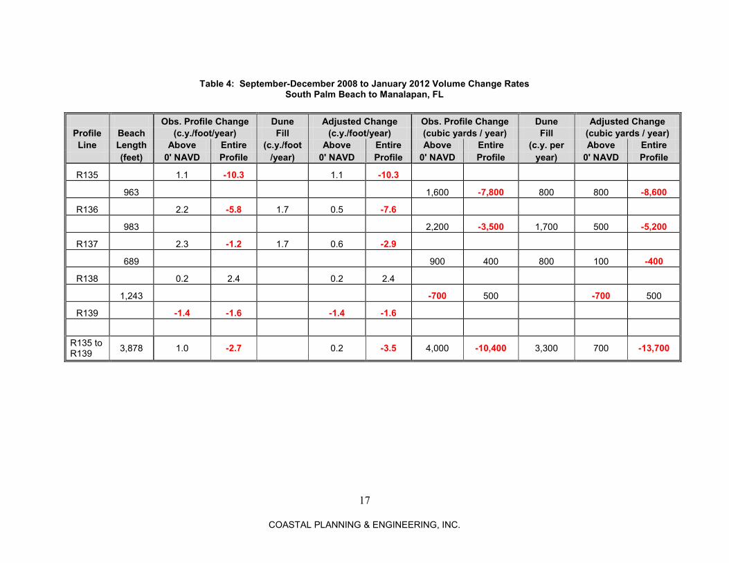
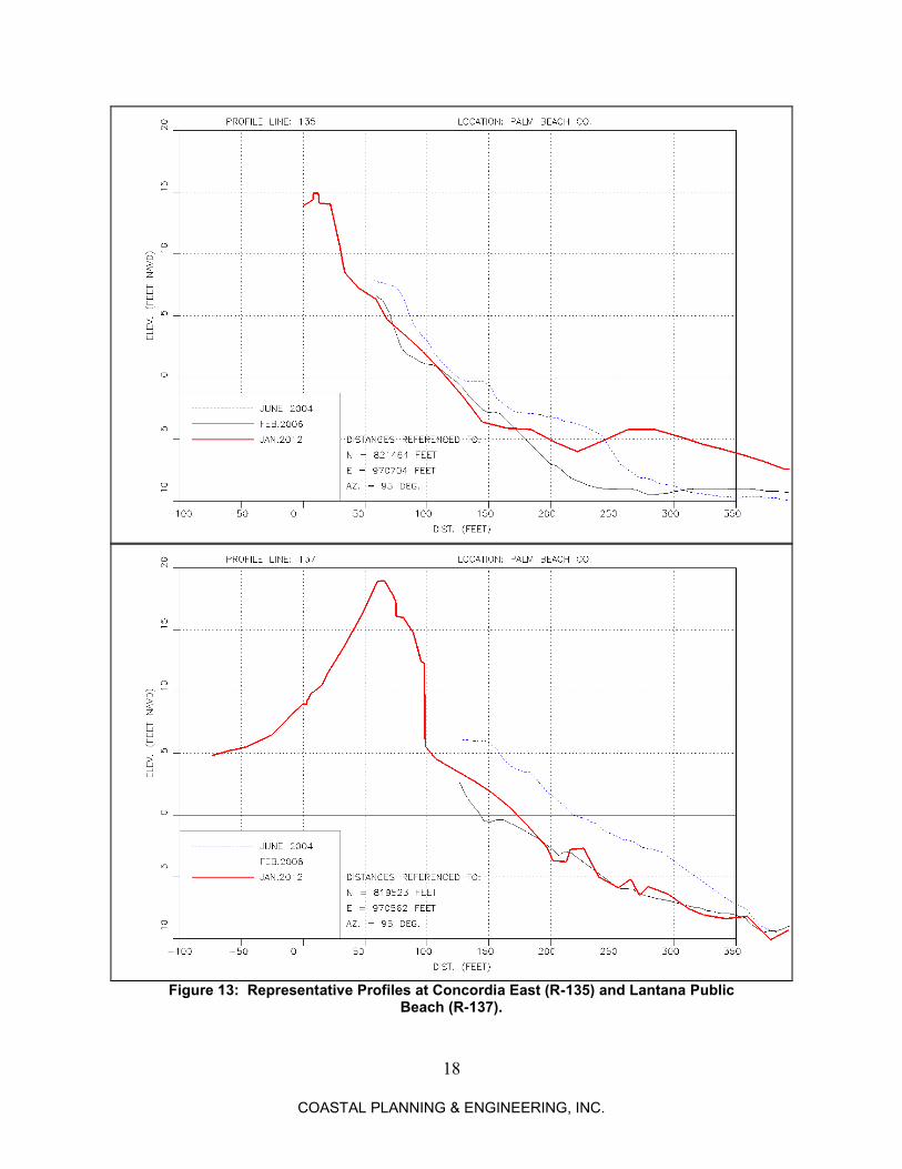
Shoreline and volume changes appear in Figure 11, Figure 12, and Table 4 (Note Figure 12 is also referenced on page 26 to show the erosion rates of Alternative E). Recent changes are based on the 2008, 2011, and 2012 surveys. Changes during years characterized by elevated wave and storm activity are based on the 2004 and 2006 surveys. Both the shoreline and volume changes suggest that the erosional patterns around the project area are characterized by erosion waves (see also CPE, 2007b), or alternating areas of erosion and accretion that move down the beach over time. Although the project area’s beaches have grown wider since 2008, the long-term trend is erosional (see Figure 11 and Figure 13). Over the beach profile as a whole, the net volume change since 2008 is a loss of 13,700 c.y./year between R-135 (Concordia East) and R-139 (Manalapan Town Hall) (see Table 4). The area that appears to be most susceptible to erosion is Lantana Public Beach (R-137), which experienced the highest losses within the project area during the 2004 and 2005 hurricane seasons.

15


Figure 11: Recent Mean High Water (+0.45’ NAVD) Shoreline Changes.

Shoreline Retreat (-) / Advance (+feet/year)

16


Figure 12: Recent Volume Changes.

17


Table 4: September-December 2008 to January 2012 Volume Change Rates

South Palm Beach to Manalapan, FL Obs. Profile Change Dune Adjusted Change Obs. Profile Change Dune Adjusted Change Profile Beach (c.y./foot/year) Fill (c.y./foot/year) (cubic yards / year) Fill (cubic yards / year) Line Length Above Entire (c.y./foot Above Entire Above Entire (c.y. per Above Entire

(feet) 0' NAVD Profile /year) 0' NAVD Profile 0' NAVD Profile year) 0' NAVD Profile

R135

1.1 -10.3

1.1 -10.3

963 1,600 -7,800 800 800 -8,600

R136 2.2 -5.8 1.7 0.5 -7.6

983 2,200 -3,500 1,700 500 -5,200

R137 2.3 -1.2 1.7 0.6 -2.9

689 900 400 800 100 -400

R138 0.2 2.4

0.2 2.4

1,243 -700 500 -700 500

R139 -1.4 -1.6

-1.4 -1.6

R135 to R139 3,878 1.0 -2.7 0.2 -3.5 4,000 -10,400 3,300 700 -13,700

18


Figure 13: Representative Profiles at Concordia East (R-135) and Lantana Public

Beach (R-137).

19


3.0 DESIGN OF ALTERNATIVES A. No-Action

Alternative A, the No-Action Scenario, is the default plan and serves as the basis for comparison with other alternatives. Under the No-Action Scenario, no further projects would be constructed by the County. The project area might benefit from littoral drift out of the various projects to the north (see Section 2.2, Figure 9, Figure 10, and Table 2). However:

Construction of these projects is not certain. In particular, the Phipps Ocean Beach (Reach 7) Beach Renourishment has not entered the Joint Coastal Permitting process.

Excluding the Phipps project, the volumes would be relatively small.

It would take several years for the placed materials to reach the project area. Aside from the project discussed in Section 2.2, protection of the upland properties from erosion-related damages would be provided by the existing seawalls only. The Delft3D model study presented later in this report provides a detailed evaluation of the No-Action Scenario. B. Original 2010 Recommended Plan

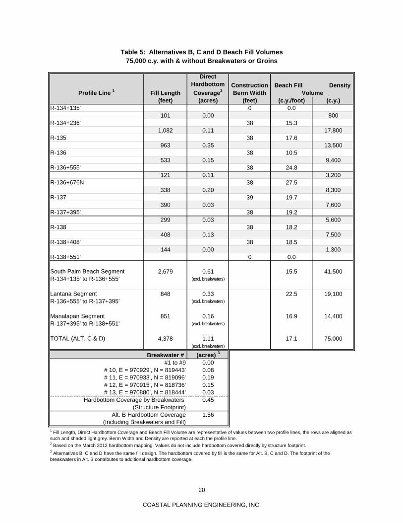
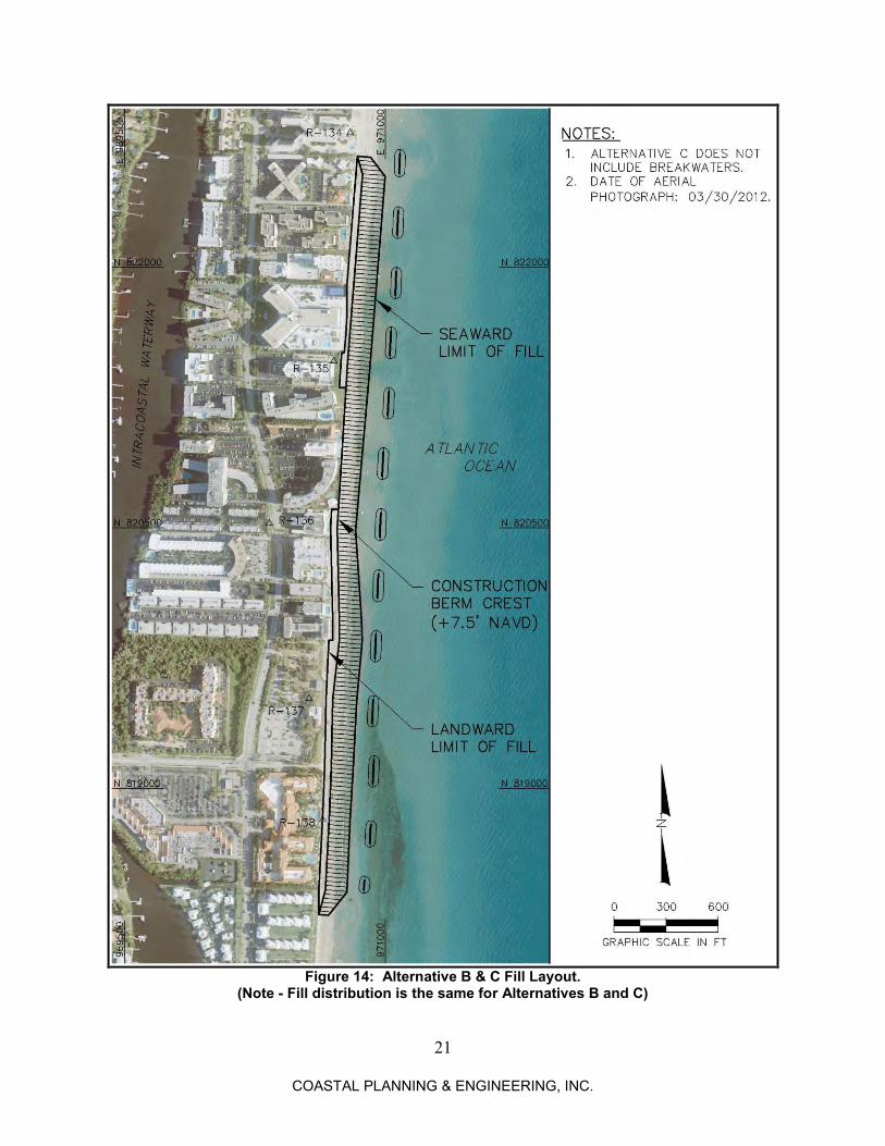
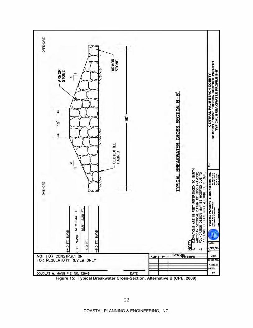
Alternative B includes 13 breakwaters and 75,000 cubic yards of fill material along the project area (see Table 5). A plan view of the alternative appears in Figure 14, with a typical breakwater cross-section appearing in Figure 15. The development of the breakwaters’ dimensions and their layout is discussed in the “South Palm Beach/Lantana Joint Coastal Permit Draft, Appendix A” dated March 9, 2009 (CPE, 2009). This draft document summarizes the methodology by which the breakwaters were designed. Based on the analytical/empirical methods used in the draft permit application (CPE, 2009), the volumetric impact to the beach and dune system resulting from the structures’ salients fill would be 75,000 cubic yards. The amount of fill that would have been placed under this alternative is equal to that volume. As noted earlier, the County is now seeking a fill design without breakwaters to last 2 to 3 years. Thus, the primary purpose of evaluating Alternative B is to compare the performance and impact of the study alternatives to the plan that was originally developed. The Delft3D model study presented later in this report provides a detailed evaluation of Alternative B in comparison to the No-Action Scenario and the other alternatives discussed below.

Table 5: Alternatives B, C and D Beach Fill Volumes75,000 c.y. with & without Breakwaters or Groins

Profile Line 1 Fill Length

Direct Hardbottom

Coverage2Construction Berm Width

Beach Fill Density Volume

(feet) (acres) (feet) (c.y./foot) (c.y.)R-134+135' 0 0.0

101 0.00 800R-134+236' 38 15.3

1,082 0.11 17,800R-135 38 17.6

963 0.35 13,500R-136 38 10.5

533 0.15 9,400R-136+555' 38 24.8

121 0.11 3,200R-136+676N 38 27.5

338 0.20 8,300R-137 39 19.7

390 0.03 7,600R-137+395' 38 19.2

299 0.03 5,600R-138 38 18.2

408 0.13 7,500R-138+408' 38 18.5

144 0.00 1,300R-138+551' 0 0.0

South Palm Beach Segment 2,679 0.61 15.5 41,500R-134+135' to R-136+555' (excl. breakwaters)

Lantana Segment 848 0.33 22.5 19,100R-136+555' to R-137+395' (excl. breakwaters)

Manalapan Segment 851 0.16 16.9 14,400R-137+395' to R-138+551' (excl. breakwaters)

TOTAL (ALT. C & D) 4,378 1.11 17.1 75,000(excl. breakwaters)

Breakwater # (acres) 3

#1 to #9 0.00# 10, E = 970929', N = 819443' 0.08# 11, E = 970933', N = 819096' 0.19# 12, E = 970915', N = 818736' 0.15# 13, E = 970880', N = 818444' 0.03

Hardbottom Coverage by Breakwaters 0.45(Structure Footprint)

Alt. B Hardbottom Coverage 1.56(Including Breakwaters and Fill)

2 Based on the March 2012 hardbottom mapping. Values do not include hardbottom covered directly by structure footprint. 3 Alternatives B, C and D have the same fill design. The hardbottom covered by fill is the same for Alt. B, C and D. The footprint of the breakwaters in Alt. B contributes to additional hardbottom coverage.

1 Fill Length, Direct Hardbottom Coverage and Beach Fill Volume are representative of values between two profile lines, the rows are aligned as such and shaded light grey. Berm Width and Density are reported at each the profile line.

20

COASTAL PLANNING ENGINEERING, INC.

21


Figure 14: Alternative B & C Fill Layout.

(Note - Fill distribution is the same for Alternatives B and C)

22


Figure 15: Typical Breakwater Cross-Section, Alternative B (CPE, 2009).

23


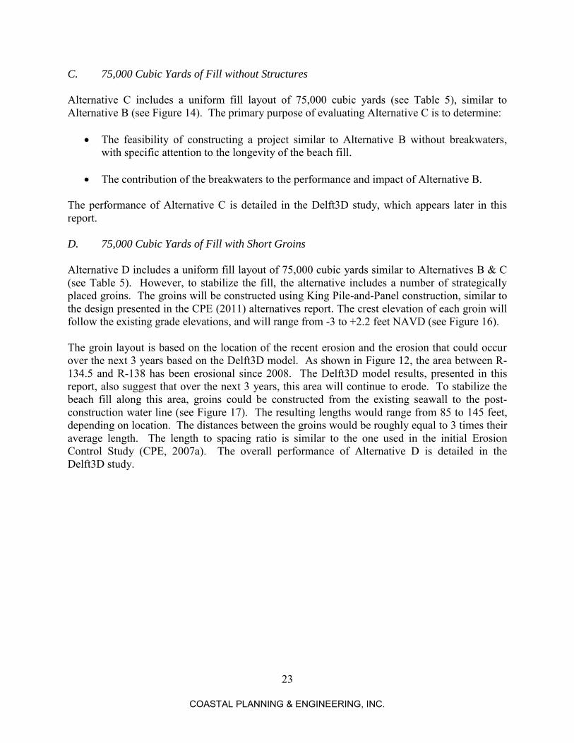
C. 75,000 Cubic Yards of Fill without Structures

Alternative C includes a uniform fill layout of 75,000 cubic yards (see Table 5), similar to Alternative B (see Figure 14). The primary purpose of evaluating Alternative C is to determine:

The feasibility of constructing a project similar to Alternative B without breakwaters, with specific attention to the longevity of the beach fill.

The contribution of the breakwaters to the performance and impact of Alternative B.

The performance of Alternative C is detailed in the Delft3D study, which appears later in this report. D. 75,000 Cubic Yards of Fill with Short Groins

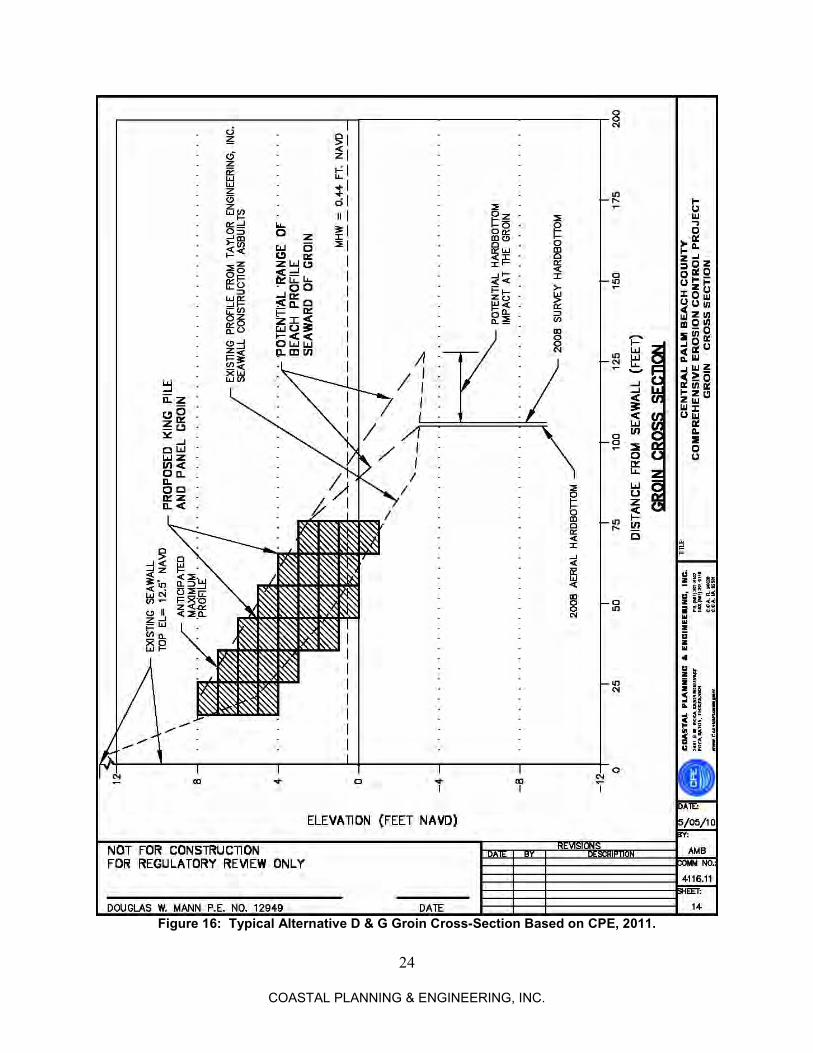
Alternative D includes a uniform fill layout of 75,000 cubic yards similar to Alternatives B & C (see Table 5). However, to stabilize the fill, the alternative includes a number of strategically placed groins. The groins will be constructed using King Pile-and-Panel construction, similar to the design presented in the CPE (2011) alternatives report. The crest elevation of each groin will follow the existing grade elevations, and will range from -3 to +2.2 feet NAVD (see Figure 16). The groin layout is based on the location of the recent erosion and the erosion that could occur over the next 3 years based on the Delft3D model. As shown in Figure 12, the area between R-134.5 and R-138 has been erosional since 2008. The Delft3D model results, presented in this report, also suggest that over the next 3 years, this area will continue to erode. To stabilize the beach fill along this area, groins could be constructed from the existing seawall to the post-construction water line (see Figure 17). The resulting lengths would range from 85 to 145 feet, depending on location. The distances between the groins would be roughly equal to 3 times their average length. The length to spacing ratio is similar to the one used in the initial Erosion Control Study (CPE, 2007a). The overall performance of Alternative D is detailed in the Delft3D study.

24


Figure 16: Typical Alternative D & G Groin Cross-Section Based on CPE, 2011.

25


Figure 17: Alternative D Groin & Fill Layout.

26


E. Fill Able to Last 3 Years without Any Structures

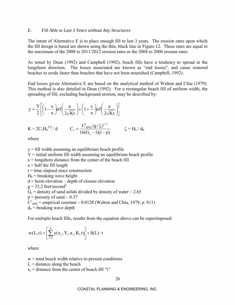
The intent of Alternative E is to place enough fill to last 3 years. The erosion rates upon which the fill design is based are shown using the thin, black line in Figure 12. These rates are equal to the maximum of the 2008 to 2011/2012 erosion rates or the 2004 to 2006 erosion rates. As noted by Dean (1992) and Campbell (1992), beach fills have a tendency to spread in the longshore direction. The losses associated are known as “end losses”, and cause restored beaches to erode faster than beaches that have not been nourished (Campbell, 1992). End losses given Alternative E are based on the analytical method of Walton and Chiu (1979). This method is also detailed in Dean (1992). For a rectangular beach fill of uniform width, the spreading of fill, excluding background erosion, may be described by:

Kt2aerf

ax1

Kt2aerf

ax1

2Yy

K = 2C1Hb5/2 / d

)p1)(1G(16)/g('C

Cs

2/1SPM

1

= Hb / db

where y = fill width assuming an equilibrium beach profile Y = initial uniform fill width assuming an equilibrium beach profile x = longshore distance from the center of the beach fill a = half the fill length t = time elapsed since construction Hb = breaking wave height d = berm elevation – depth of closure elevation g = 32.2 feet/second2 Gs = density of sand solids divided by density of water ~ 2.65 p = porosity of sand ~ 0.37 C’spm = empirical constant ~ 0.0128 (Walton and Chiu, 1979, p. 811) db = breaking wave depth For multiple beach fills, results from the equation above can be superimposed:

t)L(S)t,K,a,Y,x(y)t,L(wN

1iiii

where w = total beach width relative to present conditions L = distance along the beach xi = distance from the center of beach fill “i”

27


Yi = initial fill width of beach fill “i” ai = half the fill length of beach fill “i” S = background shoreline change rate (+ advance / − retreat) For a non-uniform beach fill, the fill layout can be divided into N individual beach fills with an ai value of L/2 and a Yi value of w(L, t=0). Figure 18 illustrates the application of the discrete solution for a triangular beach fill, a layout for which an analytical spreading solution is also available (Walton and Chiu, 1979).

Figure 18: Comparison of the Discrete and Analytical Solutions for a Triangular

Beach Fill. The Walton and Chiu (1979) method utilizes several parameters that are site-specific. The density of the sand solids is based on a typical value for sands, Gs = 2.65. Likewise, a typical porosity value of 37 percent (p = 0.37) is assumed. The berm elevation is set to +8.4 feet MSL (+7.5 feet NAVD), and a -22.6 foot MSL (-23.5 feet NAVD) depth of closure is assumed (see CPE, 2007b, 2000). The breaking wave height and corresponding depth were based on the 1989-1991 measurements at the Lake Worth Pier (USACE, 1991; CPE, 2007b). Given the entire record, the root mean square wave height was 2.2 feet, with a peak period averaging 7.3 seconds and an energy propagation vector averaging 75 degrees (east-northeast). This wave was then refracted from the

(Background shoreline change = 0 feet/year)

28


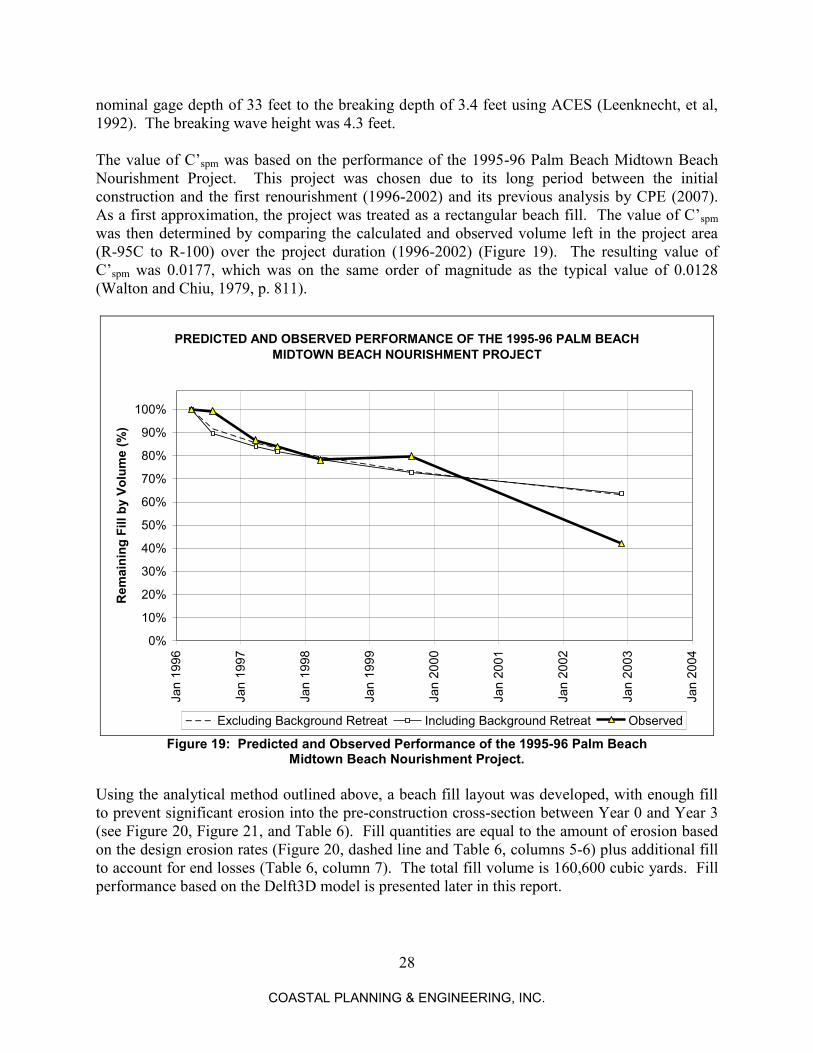
nominal gage depth of 33 feet to the breaking depth of 3.4 feet using ACES (Leenknecht, et al, 1992). The breaking wave height was 4.3 feet. The value of C’spm was based on the performance of the 1995-96 Palm Beach Midtown Beach Nourishment Project. This project was chosen due to its long period between the initial construction and the first renourishment (1996-2002) and its previous analysis by CPE (2007). As a first approximation, the project was treated as a rectangular beach fill. The value of C’spm was then determined by comparing the calculated and observed volume left in the project area (R-95C to R-100) over the project duration (1996-2002) (Figure 19). The resulting value of C’spm was 0.0177, which was on the same order of magnitude as the typical value of 0.0128 (Walton and Chiu, 1979, p. 811).

PREDICTED AND OBSERVED PERFORMANCE OF THE 1995-96 PALM BEACH MIDTOWN BEACH NOURISHMENT PROJECT

0%

10%

20%

30%

40%

50%

60%

70%

80%

90%

100%

Jan

1996

Jan

1997

Jan

1998

Jan

1999

Jan

2000

Jan

2001

Jan

2002

Jan

2003

Jan

2004

Rem

aini

ng F

ill b

y Vo

lum

e (%

)

Excluding Background Retreat Including Background Retreat Observed

Figure 19: Predicted and Observed Performance of the 1995-96 Palm Beach Midtown Beach Nourishment Project.

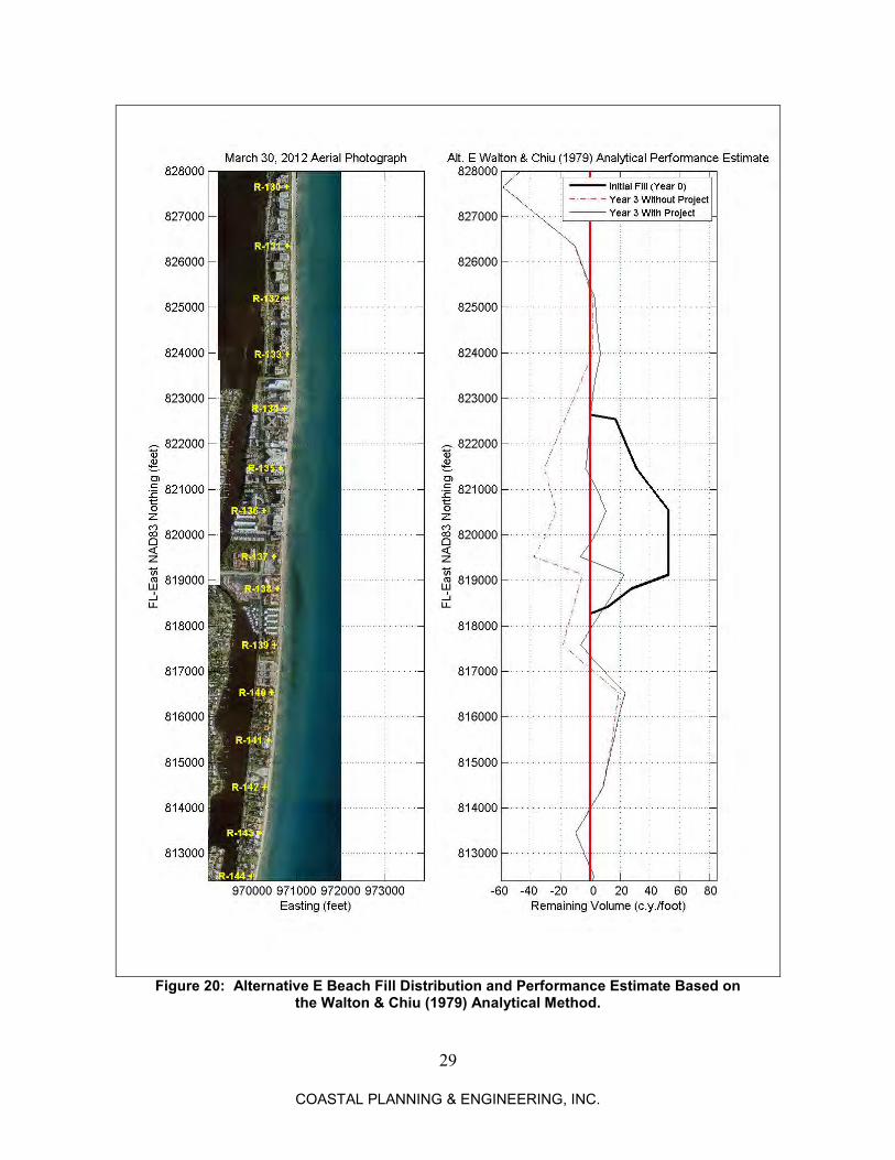
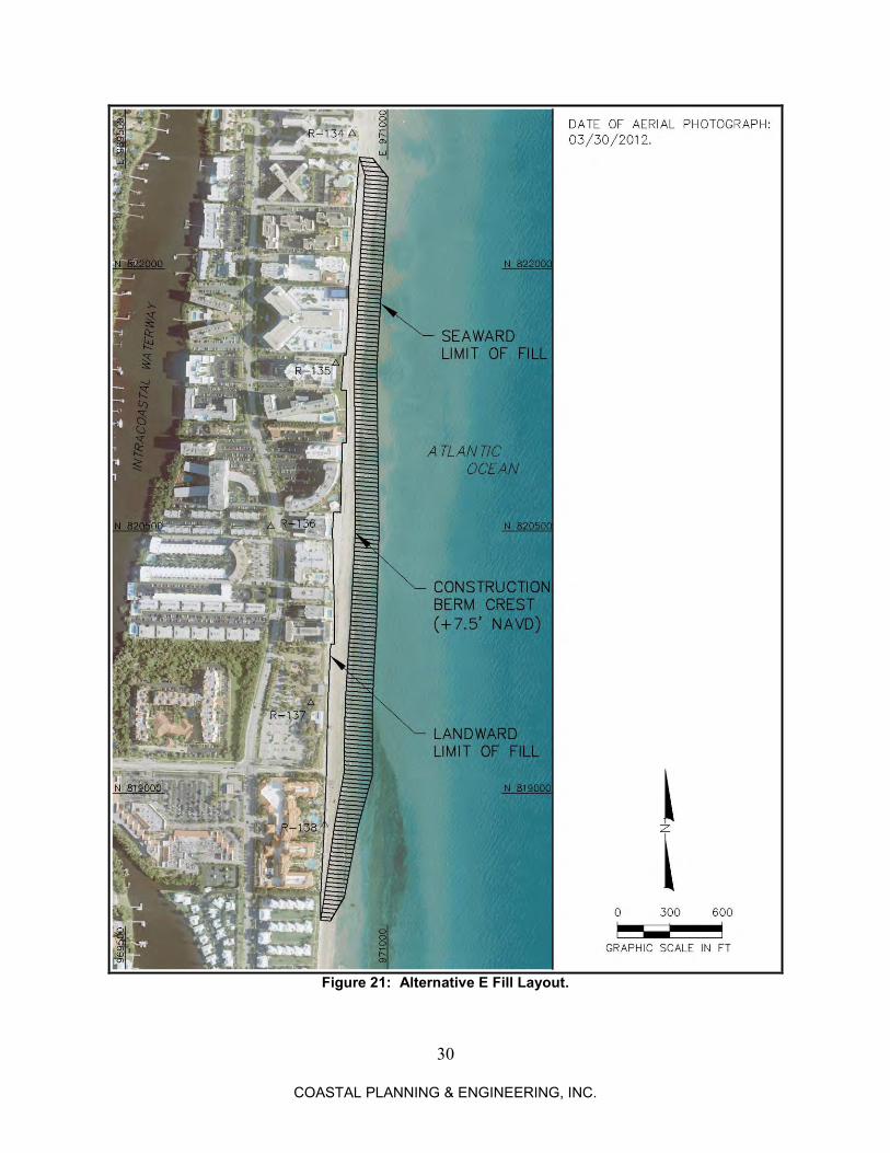
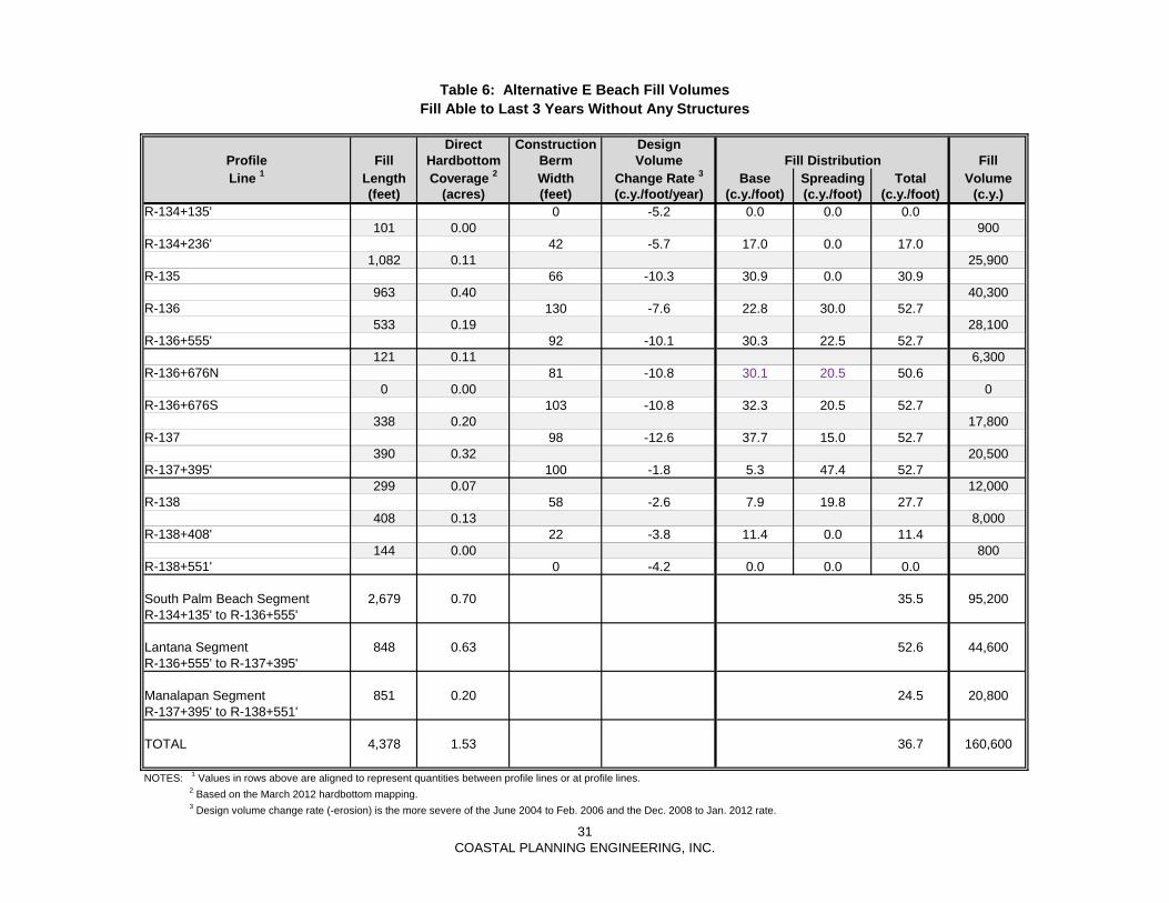
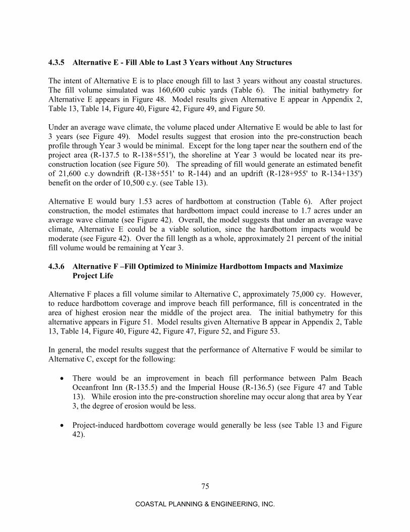
Using the analytical method outlined above, a beach fill layout was developed, with enough fill to prevent significant erosion into the pre-construction cross-section between Year 0 and Year 3 (see Figure 20, Figure 21, and Table 6). Fill quantities are equal to the amount of erosion based on the design erosion rates (Figure 20, dashed line and Table 6, columns 5-6) plus additional fill to account for end losses (Table 6, column 7). The total fill volume is 160,600 cubic yards. Fill performance based on the Delft3D model is presented later in this report.

29


Figure 20: Alternative E Beach Fill Distribution and Performance Estimate Based on

the Walton & Chiu (1979) Analytical Method.

30


Figure 21: Alternative E Fill Layout.

Table 6: Alternative E Beach Fill VolumesFill Able to Last 3 Years Without Any Structures

Direct Construction DesignProfile Fill Hardbottom Berm Volume Fill Distribution FillLine 1 Length Coverage 2 Width Change Rate 3 Base Spreading Total Volume

(feet) (acres) (feet) (c.y./foot/year) (c.y./foot) (c.y./foot) (c.y./foot) (c.y.)R-134+135' 0 -5.2 0.0 0.0 0.0

101 0.00 900R-134+236' 42 -5.7 17.0 0.0 17.0

1,082 0.11 25,900R-135 66 -10.3 30.9 0.0 30.9

963 0.40 40,300R-136 130 -7.6 22.8 30.0 52.7

533 0.19 28,100R-136+555' 92 -10.1 30.3 22.5 52.7

121 0.11 6,300R-136+676N 81 -10.8 30.1 20.5 50.6

0 0.00 0R-136+676S 103 -10.8 32.3 20.5 52.7

338 0.20 17,800R-137 98 -12.6 37.7 15.0 52.7

390 0.32 20,500R-137+395' 100 -1.8 5.3 47.4 52.7

299 0.07 12,000R-138 58 -2.6 7.9 19.8 27.7

408 0.13 8,000R-138+408' 22 -3.8 11.4 0.0 11.4

144 0.00 800R-138+551' 0 -4.2 0.0 0.0 0.0

South Palm Beach Segment 2,679 0.70 35.5 95,200R-134+135' to R-136+555'

Lantana Segment 848 0.63 52.6 44,600R-136+555' to R-137+395'

Manalapan Segment 851 0.20 24.5 20,800R-137+395' to R-138+551'

TOTAL 4,378 1.53 36.7 160,600

NOTES: 1 Values in rows above are aligned to represent quantities between profile lines or at profile lines.

2 Based on the March 2012 hardbottom mapping.

3 Design volume change rate (-erosion) is the more severe of the June 2004 to Feb. 2006 and the Dec. 2008 to Jan. 2012 rate.

31COASTAL PLANNING ENGINEERING, INC.

32


F. Fill Optimized to Minimize Hardbottom Impacts and Maximize Project Life

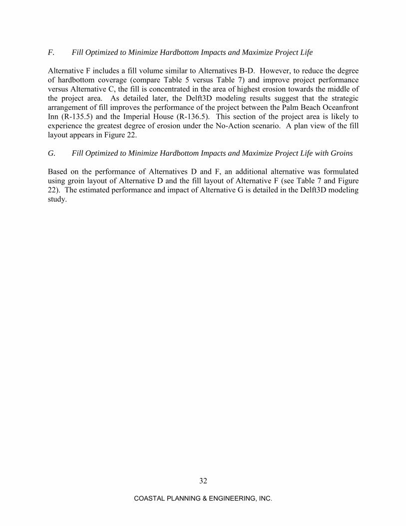
Alternative F includes a fill volume similar to Alternatives B-D. However, to reduce the degree of hardbottom coverage (compare Table 5 versus Table 7) and improve project performance versus Alternative C, the fill is concentrated in the area of highest erosion towards the middle of the project area. As detailed later, the Delft3D modeling results suggest that the strategic arrangement of fill improves the performance of the project between the Palm Beach Oceanfront Inn (R-135.5) and the Imperial House (R-136.5). This section of the project area is likely to experience the greatest degree of erosion under the No-Action scenario. A plan view of the fill layout appears in Figure 22. G. Fill Optimized to Minimize Hardbottom Impacts and Maximize Project Life with Groins

Based on the performance of Alternatives D and F, an additional alternative was formulated using groin layout of Alternative D and the fill layout of Alternative F (see Table 7 and Figure 22). The estimated performance and impact of Alternative G is detailed in the Delft3D modeling study.

33


Table 7: Alternatives F & G Beach Fill Volumes

Fill Optimized to Minimize Hardbottom Impacts and Maximize Project Life with & without Groins

Direct Construction

Profile Fill Hardbottom Berm Fill Fill Line Length Coverage* Width Distr. Volume

(feet) (acres) (feet) (c.y./foot) (c.y.) R-134+135'

0.0 0.0

101 0.00 500 R-134+236' 27.3 10.0

1,082 0.10 10,800 R-135 21.7 10.0

963 0.37 17,800 R-136 75.6 27.0

533 0.19 14,400 R-136+555' 42.9 27.0

121 0.11 3,300 R-136+676N 37.3 27.0

0 0.00 0 R-136+676S 59.7 29.1

338 0.20 9,500 R-137 52.7 27.0

390 0.02 7,200 R-137+395' 17.8 10.0

299 0.00 3,000 R-138 18.5 10.0

408 0.05 4,100 R-138+408' 19.0 10.0

144 0.00 1,400 R-138+551' 8.5 10.0

South Palm Beach Segment 2,679 0.66

16.2 43,500

R-134+135' to R-136+555' Lantana Segment 848 0.33

23.6 20,000

R-136+555' to R-137+395' Manalapan Segment 851 0.05

10.0 8,500

R-137+395' to R-138+551' TOTAL 4,378 1.04

16.4 72,000

* Based on the March 2012 hardbottom mapping.

34


Figure 22: Alternatives F & G Fill & Groin Layout.

(Note - Fill distribution is the same for Alternatives F and G)

35


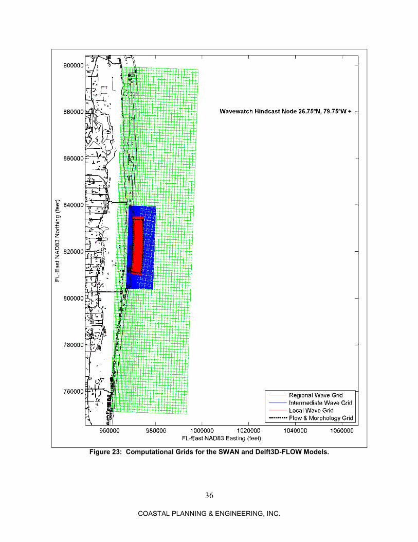
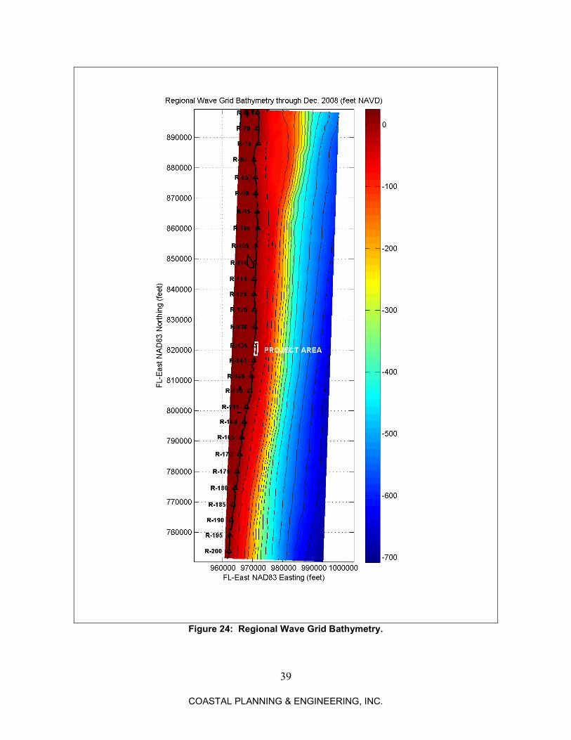
4.0 DELFT3D MODELING STUDY 4.1 General The performance and impact of each alternative was evaluated using the Delft3D morphological model (Deltares, 2011a). This model determines changes in a topographic and bathymetric surface based on the effects of waves, water levels, winds, and currents. Wave transformation from the offshore to the nearshore area is simulated using the SWAN wave transformation model (Booij, et al, 2004). The SWAN model (version 40.72ABCDE) is coupled with the Delft3D-FLOW model (version 4.00.04.757), which simulates currents, water levels, and sediment transport. Based on the sediment transport estimates at each flow time step, the Delft3D-FLOW model calculates the subsequent elevations of the topographic and bathymetric surface. Typical time steps in Delft3D-FLOW range from 1 second to 60 seconds. Water levels, currents, and bottom grade elevations are then sent to the SWAN model at each wave time step, which is on the order of 0.5 to 3 hours. 4.2 Updated Model Calibration Calibration of the SWAN model was performed using wave measurements collected near the project site in 2008. Details regarding the SWAN model calibration appear in CPE (2010). The flow parameters used in the Delft3D-FLOW model were set to the values recommended by Deltares (2011a) as detailed in Appendix 2 of CPE (2010). Sediment transport, erosion, and deposition within Delft3D-FLOW were initially calibrated using bathymetric surveys taken in 2006 and 2008 (CPE, 2010). This phase of the calibration was heavily tied to the hardbottom conditions that existed in 2006 (see CPE, 2010, pp. 36-38). As noted in the initial calibration report and other sources (CPE, 2007b), the extent of the exposed hardbottom near the project area is highly variable. Given these factors, the sediment transport, erosion, and deposition parameters in the model were recalibrated based on the volumetric erosion rates between December 2008 and January 2012 (Figure 12). 4.2.1 Grids Four different computational grids were created for numerical model calibration and production simulations (Figure 23). These grids were created for the following purposes:

Regional Wave Grid. This grid was designed to propagate wave characteristics from deep water to intermediate-shallow water and examine regional wave transformation processes.

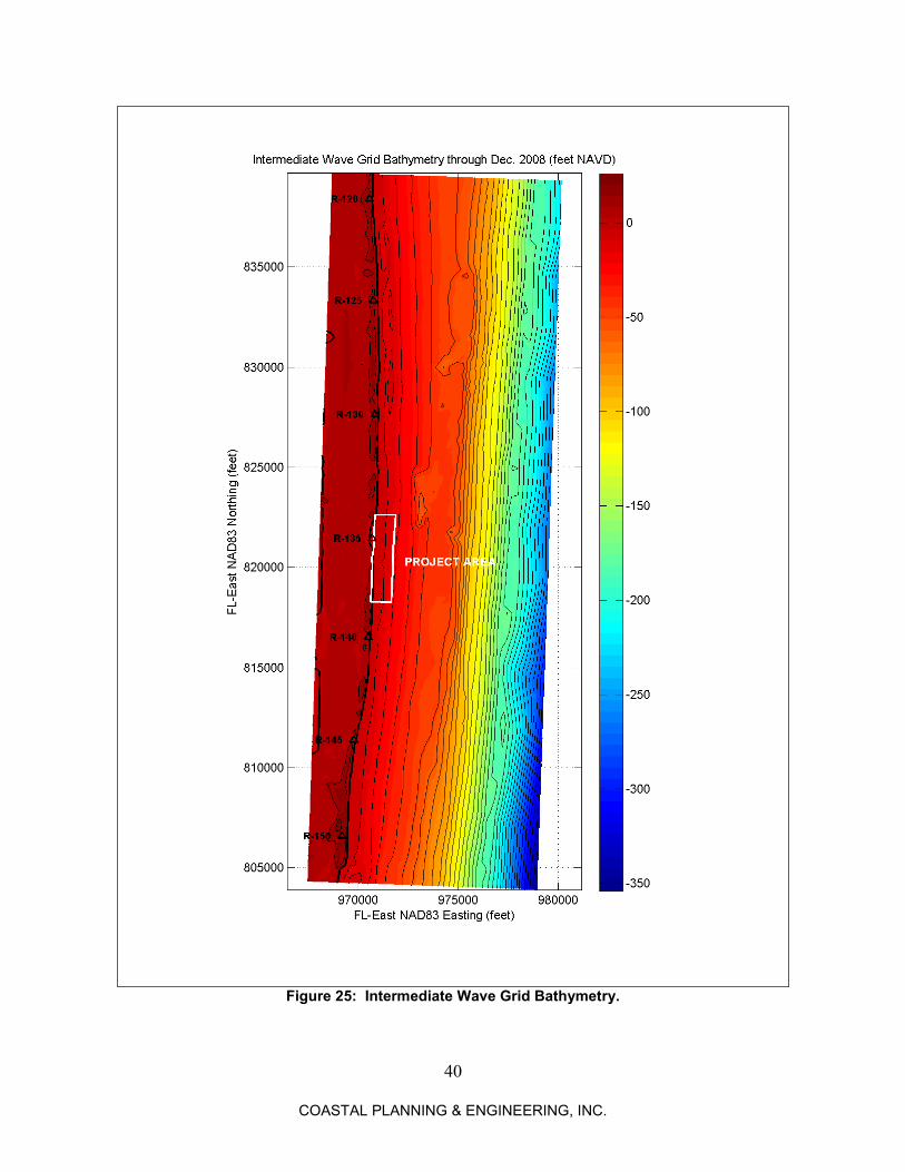
Intermediate Wave Grid. This grid was designed to transform waves between the

coarsely-spaced, Regional Wave Grid and the local, high resolution wave grid. The Intermediate Wave Grid was nested within the Regional Wave Grid.

36


Figure 23: Computational Grids for the SWAN and Delft3D-FLOW Models.

37


Local Wave Grid. This grid was designed to examine detailed, shallow water wave

propagation processes. This nearshore grid was nested within the Intermediate Wave Grid. The central area of this grid was created with sufficient resolution to simulate the refraction, diffraction, and breaking processes near the coastal structures being evaluated. The offshore boundary of the nearshore wave grids followed the -61 foot NAVD depth contour.

Flow & Morphology Grid. This grid was designed to examine circulation patterns and bathymetric changes in the project area and the adjacent beaches. This grid was merged along several rows of grid cells along the northern, southern, and eastern edges of the grid to provide for a stable coupling between the SWAN and Delft3D-FLOW models.

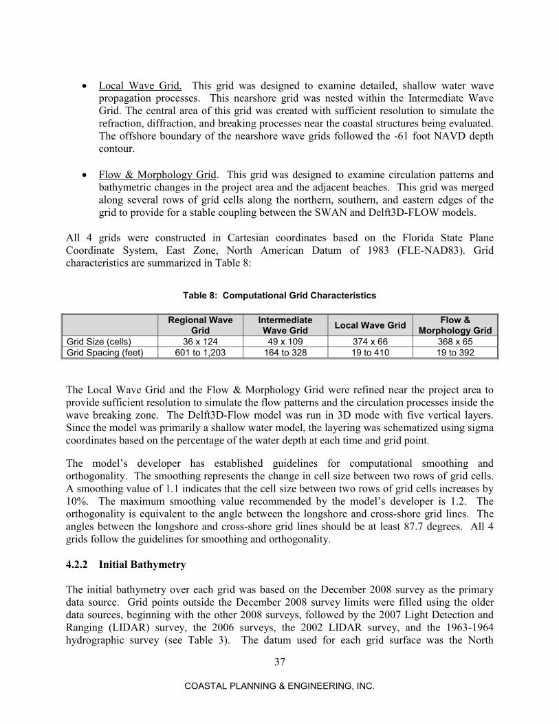
All 4 grids were constructed in Cartesian coordinates based on the Florida State Plane Coordinate System, East Zone, North American Datum of 1983 (FLE-NAD83). Grid characteristics are summarized in Table 8:

Table 8: Computational Grid Characteristics Regional Wave

Grid Intermediate Wave Grid Local Wave Grid Flow &

Morphology Grid Grid Size (cells) 36 x 124 49 x 109 374 x 66 368 x 65 Grid Spacing (feet) 601 to 1,203 164 to 328 19 to 410 19 to 392

The Local Wave Grid and the Flow & Morphology Grid were refined near the project area to provide sufficient resolution to simulate the flow patterns and the circulation processes inside the wave breaking zone. The Delft3D-Flow model was run in 3D mode with five vertical layers. Since the model was primarily a shallow water model, the layering was schematized using sigma coordinates based on the percentage of the water depth at each time and grid point. The model’s developer has established guidelines for computational smoothing and orthogonality. The smoothing represents the change in cell size between two rows of grid cells. A smoothing value of 1.1 indicates that the cell size between two rows of grid cells increases by 10%. The maximum smoothing value recommended by the model’s developer is 1.2. The orthogonality is equivalent to the angle between the longshore and cross-shore grid lines. The angles between the longshore and cross-shore grid lines should be at least 87.7 degrees. All 4 grids follow the guidelines for smoothing and orthogonality. 4.2.2 Initial Bathymetry The initial bathymetry over each grid was based on the December 2008 survey as the primary data source. Grid points outside the December 2008 survey limits were filled using the older data sources, beginning with the other 2008 surveys, followed by the 2007 Light Detection and Ranging (LIDAR) survey, the 2006 surveys, the 2002 LIDAR survey, and the 1963-1964 hydrographic survey (see Table 3). The datum used for each grid surface was the North

38


American Vertical Datum of 1988 (NAVD). Conversions to NAVD were based on the following:

For the 2002 LIDAR survey and the 2006 borrow area survey, the National Geodetic Vertical Datum of 1929 (NGVD) was assumed to be equal to -1.53 feet NAVD (NOAA, 2003).

For the 1963-1964 hydrographic offshore, the average value of the Mean Lower Low Water datum was -2.52 feet NAVD based on the NOAA (2012) VDATUM 3.1 conversion program. The horizontal conversion between latitude/longitude and FLE-NAD83 coordinates was performed using Corpscon 5.11.08.

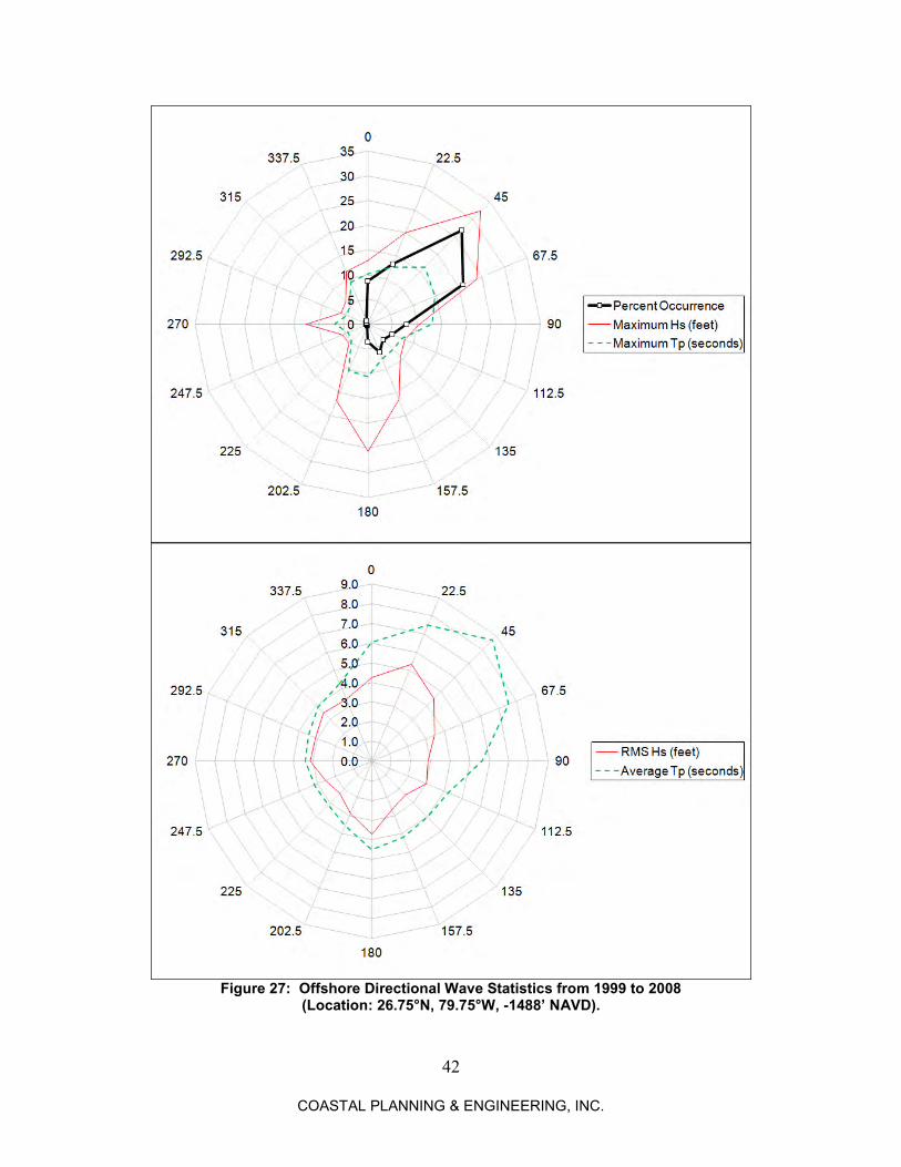
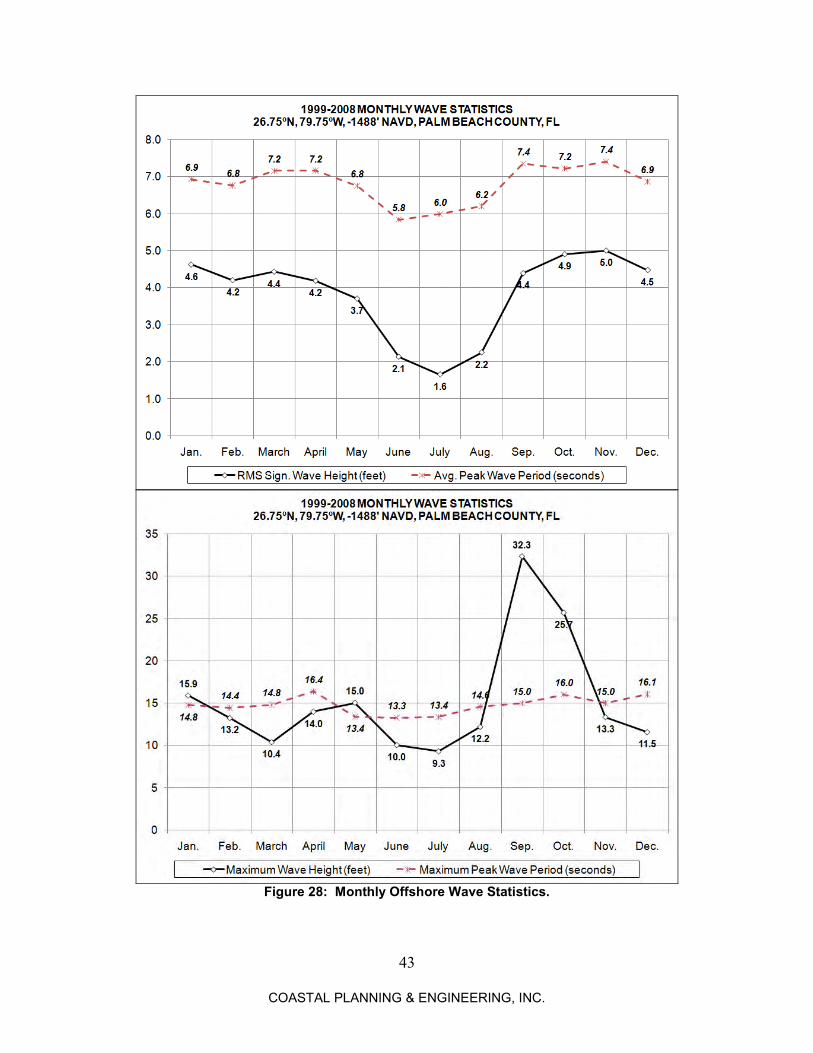
The initial bathymetry over each grid appears in Figure 24 through Figure 26. Bathymetry over the Local Wave Grid and the Flow & Morphology Grid was updated based on the estimated sediment transport. Bathymetry over the Regional Wave Grid and Intermediate Wave Grid was assumed to be constant with time. 4.2.3 Waves Waves in this study were primarily based on the NOAA (2013) WAVEWATCH hindcast for the Western North Atlantic. The hindcast data was provided in the form of grids covering the Atlantic coast of North America from 1999 to 2012. Similar to the original calibration (CPE, 2010), the WAVEWATCH waves used in the Delft3D model were taken from the forecast at 26.50ºN, 79.75ºW (see Figure 23). The depth at this site was -1,488 feet NAVD. The highest and longest waves during average conditions occur between September and January, with the lowest and shortest waves occurring between June and August. Between June and August, waves from the east and east-southeast are common. During the rest of the year, waves typically originate from the northeast. The root-mean-square wave height is on the order of 4.0 feet, with an average peak period of 6.8 seconds and an average direction of 43 degrees (from the NE). Overall, 70 percent of the wave energy originates from the northerly direction bands (0-67.5 degrees), 8 percent of the wave energy originates from the east, and 19 percent of the wave energy originates from the southerly direction bands (112.5 to 180 degrees). Directional wave statistics appear in Figure 27. Monthly wave statistics appear in Figure 28 and Figure 29. Two- and three-dimensional sediment transport and morphology models are computationally intensive. Furthermore, while flows change on an hourly basis, the morphology changes occur on a scale of months to years. For this reason, it is not practical to simulate 3-4 years of volume changes using a 3-4 year time series of offshore water levels and waves to drive the model. Instead, the Delft3D model is typically run for a shorter period of time, using 10-30 wave cases to approximate the general wave climate during the period of interest (i.e.: Lesser, et al., 2004; Benedet and List, 2008). The number of wave cases, and their characteristics, are chosen to produce sediment transport patterns that would be similar to those based on the full time series of offshore waves (i.e. 3-4 years).

39


Figure 24: Regional Wave Grid Bathymetry.

40


Figure 25: Intermediate Wave Grid Bathymetry.

41


Figure 26: Initial, 2008 Bathymetry over the Local Wave Grid & the Flow &

Morphology Grid.

PHIPPS OCEAN PARK BORROW AREAS

42


Figure 27: Offshore Directional Wave Statistics from 1999 to 2008

(Location: 26.75°N, 79.75°W, -1488’ NAVD).

43


Figure 28: Monthly Offshore Wave Statistics.

44


Figure 29: Monthly Variation of Wave Direction Offshore.

The offshore wave climate during the calibration period was based on the time series of WAVEWATCH waves at 26.75°N, 79.75°W between December 2008 and January 2012. The primary wave cases were selected from the waves originating from the seaward direction bands (0 to 180°), which covered 82 percent of the wave record by time. These wave records were divided into wave height and direction classes, with each wave class containing an equal amount of wave energy (in KW-Hours/m or Joules/m). This method, known as the Energy Flux Method, characterized each wave record based on the energy flux:

P = ECg = wave energy in watts per m Energy per wave record (Joules per m) = Pt where:

E = gHs2 = wave energy in Joules per m2

(3,600,000 Joules = 1 KW-hour)

Cgn = (1/2) (L/Tp){ 1 + [(4d/L)/sinh(4d/L)] } = group wave velocity in m/s

45


L = [gTp2/(2)] tanh(2d/L) = wavelength in m

and:

= seawater density = 1,025 kg/m3 (63.99 lbm/foot3) g = gravity = 9.81 m/s2 (32.2 feet/s2)

Hs = significant wave height in m Tp = peak wave period in seconds d = depth = 453 m (1,488 feet) t = interval between wave records = 10,800 seconds (3 hours)

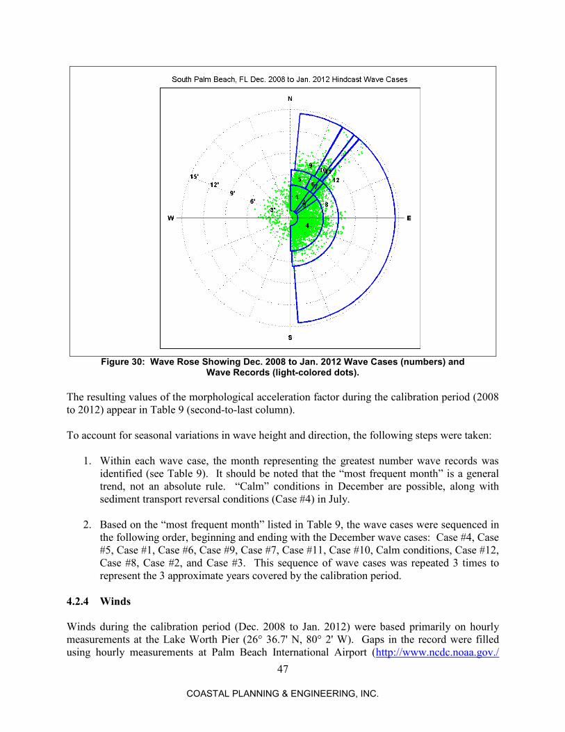
Based on the energy estimates above, the offshore waves (0 to 180°) were divided into 3 height classes with roughly equal amounts of wave energy in KW-Hours/m. Each height class was then divided into 4 direction bands representing equal amounts of wave energy, for a total of 12 wave cases (see Table 9 and Figure 30). To account for periods during which the offshore waves were propagating from the landward directions (180 to 360°), a 13th wave case was added, representing calm conditions. Excluding the calm case, each wave case at 26.75°N, 79.75°W represented a nearly equal amount of wave energy. However, since higher, more energetic waves occurred less often than lower waves, the various wave cases did not represent an equal portion of the wave record with respect to time (% occurrence). Directional spreading values offshore were assumed to be equal to the model’s default value of 25 degrees. The wave measurements taken in 2008 did not support the use of narrower directional spreading values for medium or long-period (Tp > 5 sec.) waves. To decrease the time needed for the morphological computation, morphological acceleration factors were used, as described in Lesser et al (2004) and Benedet and List (2008). The morphological acceleration factor M was estimated according to the following:

M = Tstudy period / Tmodel period

where

Tstudy period = (length of the study period) x (percent occurrence for each wave case) Tmodel period = duration of the wave case in the model simulation

For example, a wave case that occurs 14 days a year can be simulated over 24 hours with an M value of 14. With the Delft3D modeling community, it is common practice to use lower M values for high wave cases, when the most significant morphological changes occur, and higher M values for smaller wave cases, where little change takes place. Over the calibration period, the values of Tmodel period were equal to the following:

Calm Case and Wave Cases #1 to #4: 9 tide cycles (3 per year), 111.6 hours. Wave Cases #5 to #8: 6 tide cycles (3 per year), 74.4 hours. Wave Cases #9 to #12: 3 tide cycles (1 per year), 37.2 hours.

46


Table 9: Dec. 2008 to Jan. 2012 Wave Climate A 26.75ºN, 79.75ºW, -1,488 feet NAVD

Central Palm Beach County, FL

Case #

RMS Sign. Wave Height (feet)

Avg. Peak Wave Period (sec.)

Avg. Peak Wave

Direction (deg.)

Avg. Wind

Speed (mph)

Avg. Wind Direction

(deg.)

% Occur- rence

Height Class (feet)

Direction Band (deg.)

Month Freq.

Month

Dec. 2008 to Jan. 2012 Morpho- logical Accel. Factor

5-Year Morpho- logical Accel. Factor

1 3.1 6.6 19 11.5 1 13.1% 1.0 to 4.6 0 to 35 Dec. 31.8 30.8 2 2.9 8.8 40 10.5 189 11.3% 1.0 to 4.6 35 to 44 Dec. 27.6 26.7 3 2.7 9.6 48 10.4 111 12.3% 1.0 to 4.6 44 to 55 Dec. 29.9 28.9 4 2.6 4.7 113 14.8 153 27.1% 1.0 to 4.6 55 to 180 Dec. 65.8 63.8

5 5.5 7.3 14 12.4 352 3.7% 4.6 to 6.7 1 to 27 Dec. 13.4 13.0 6 5.6 8.8 34 12.4 67 2.9% 4.6 to 6.7 27 to 37 Jan. 10.7 10.4 7 5.6 9.5 40 13.4 96 2.7% 4.6 to 6.7 37 to 43 Feb. 9.8 9.5 8 5.4 7.0 70 17.4 96 4.1% 4.6 to 6.7 44 to 178 Dec. 14.8 14.4

9 7.8 8.3 21 15.9 26 1.6% 6.7 to 14.5 5 to 30 Jan. 11.5 11.2 10 8.0 9.3 35 15.7 65 1.3% 6.7 to 14.5 30 to 38 April 9.4 9.1 11 8.3 10.5 39 14.2 72 1.1% 6.7 to 14.5 38 to 41 March 7.7 7.5 12 8.2 8.8 50 20.6 61 1.3% 6.7 to 14.5 41 to 176 Nov. 9.4 9.1

CALM 1.6 7.2 58 9.8 253 17.6% All Remaining Waves July 42.9 41.6

47


Figure 30: Wave Rose Showing Dec. 2008 to Jan. 2012 Wave Cases (numbers) and

Wave Records (light-colored dots). The resulting values of the morphological acceleration factor during the calibration period (2008 to 2012) appear in Table 9 (second-to-last column). To account for seasonal variations in wave height and direction, the following steps were taken:

1. Within each wave case, the month representing the greatest number wave records was identified (see Table 9). It should be noted that the “most frequent month” is a general trend, not an absolute rule. “Calm” conditions in December are possible, along with sediment transport reversal conditions (Case #4) in July.

2. Based on the “most frequent month” listed in Table 9, the wave cases were sequenced in the following order, beginning and ending with the December wave cases: Case #4, Case #5, Case #1, Case #6, Case #9, Case #7, Case #11, Case #10, Calm conditions, Case #12, Case #8, Case #2, and Case #3. This sequence of wave cases was repeated 3 times to represent the 3 approximate years covered by the calibration period.

4.2.4 Winds Winds during the calibration period (Dec. 2008 to Jan. 2012) were based primarily on hourly measurements at the Lake Worth Pier (26° 36.7' N, 80° 2' W). Gaps in the record were filled using hourly measurements at Palm Beach International Airport (http://www.ncdc.noaa.gov./

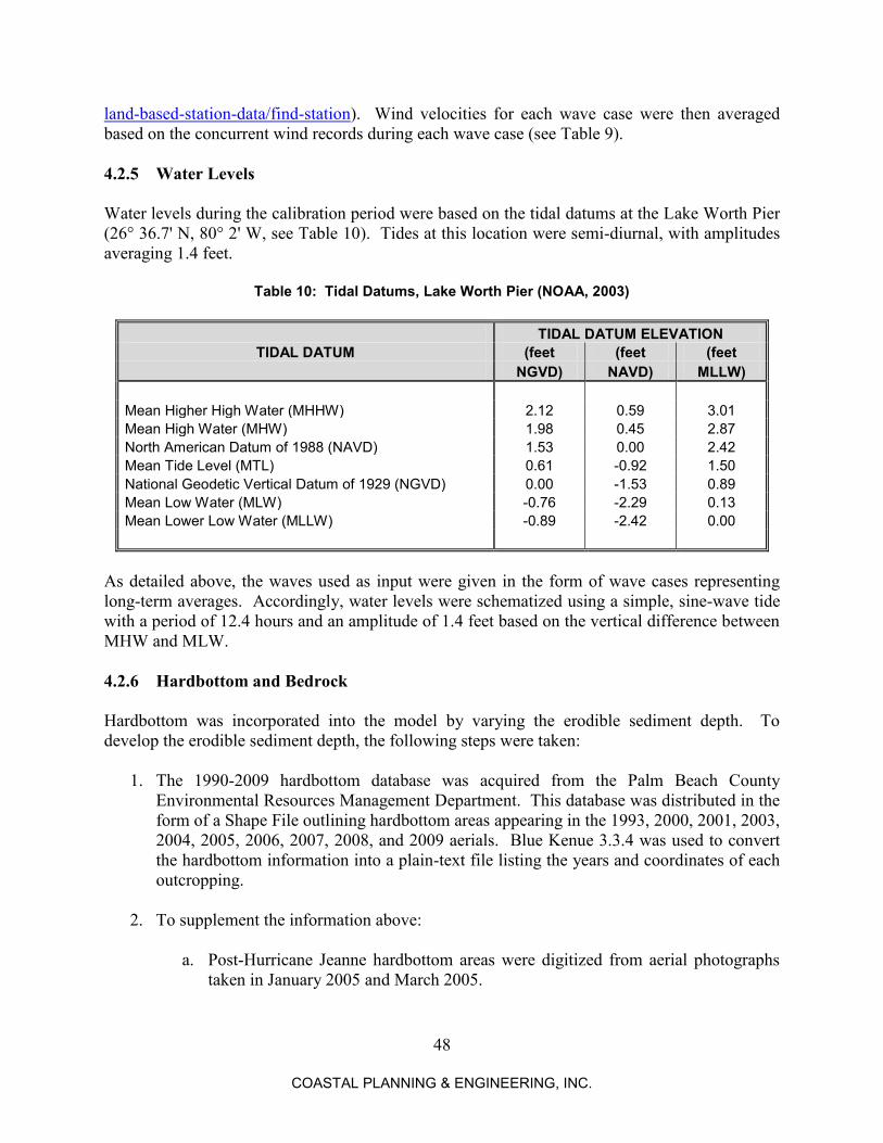
http://www.ncdc.noaa.gov./%20land-based-station-data/find-station

48


land-based-station-data/find-station). Wind velocities for each wave case were then averaged based on the concurrent wind records during each wave case (see Table 9). 4.2.5 Water Levels Water levels during the calibration period were based on the tidal datums at the Lake Worth Pier (26° 36.7' N, 80° 2' W, see Table 10). Tides at this location were semi-diurnal, with amplitudes averaging 1.4 feet.

Table 10: Tidal Datums, Lake Worth Pier (NOAA, 2003)

TIDAL DATUM ELEVATION TIDAL DATUM (feet (feet (feet

NGVD) NAVD) MLLW) Mean Higher High Water (MHHW) 2.12 0.59 3.01 Mean High Water (MHW) 1.98 0.45 2.87 North American Datum of 1988 (NAVD) 1.53 0.00 2.42 Mean Tide Level (MTL) 0.61 -0.92 1.50 National Geodetic Vertical Datum of 1929 (NGVD) 0.00 -1.53 0.89 Mean Low Water (MLW) -0.76 -2.29 0.13 Mean Lower Low Water (MLLW) -0.89 -2.42 0.00

As detailed above, the waves used as input were given in the form of wave cases representing long-term averages. Accordingly, water levels were schematized using a simple, sine-wave tide with a period of 12.4 hours and an amplitude of 1.4 feet based on the vertical difference between MHW and MLW. 4.2.6 Hardbottom and Bedrock Hardbottom was incorporated into the model by varying the erodible sediment depth. To develop the erodible sediment depth, the following steps were taken:

1. The 1990-2009 hardbottom database was acquired from the Palm Beach County Environmental Resources Management Department. This database was distributed in the form of a Shape File outlining hardbottom areas appearing in the 1993, 2000, 2001, 2003, 2004, 2005, 2006, 2007, 2008, and 2009 aerials. Blue Kenue 3.3.4 was used to convert the hardbottom information into a plain-text file listing the years and coordinates of each outcropping.

2. To supplement the information above:

a. Post-Hurricane Jeanne hardbottom areas were digitized from aerial photographs taken in January 2005 and March 2005.

http://www.ncdc.noaa.gov./%20land-based-station-data/find-station

49


b. Nearshore hardbottom areas were digitized from December 2002 aerials provided by the U.S. Geological Survey (USGS) Earth Explorer. These hardbottom areas were combined with 2002 offshore hardbottom mapping provided by the Florida Fish and Wildlife Conservation Commission (FFWCC, http://ocean.floridamarine.org/mrgis/Description_Layers_Marine.htm).

c. The 1993 hardbottom mapping from FFWCC was combined with the 1993 hardbottom mapping from the Palm Beach County database.

d. The March 2012 hardbottom mapping was digitized from March 2012 aerial

photographs flown by Aerial Cartographics of America on behalf of the Town of Palm Beach and FDEP. The quality of the photographs and the water clarity during the flight date was sufficient for this purpose (for example, see Figure 14). Although the Town of Palm Beach was the sponsor of these photographs, they provided full coverage of the model grids shown in Figure 26, including the project area.

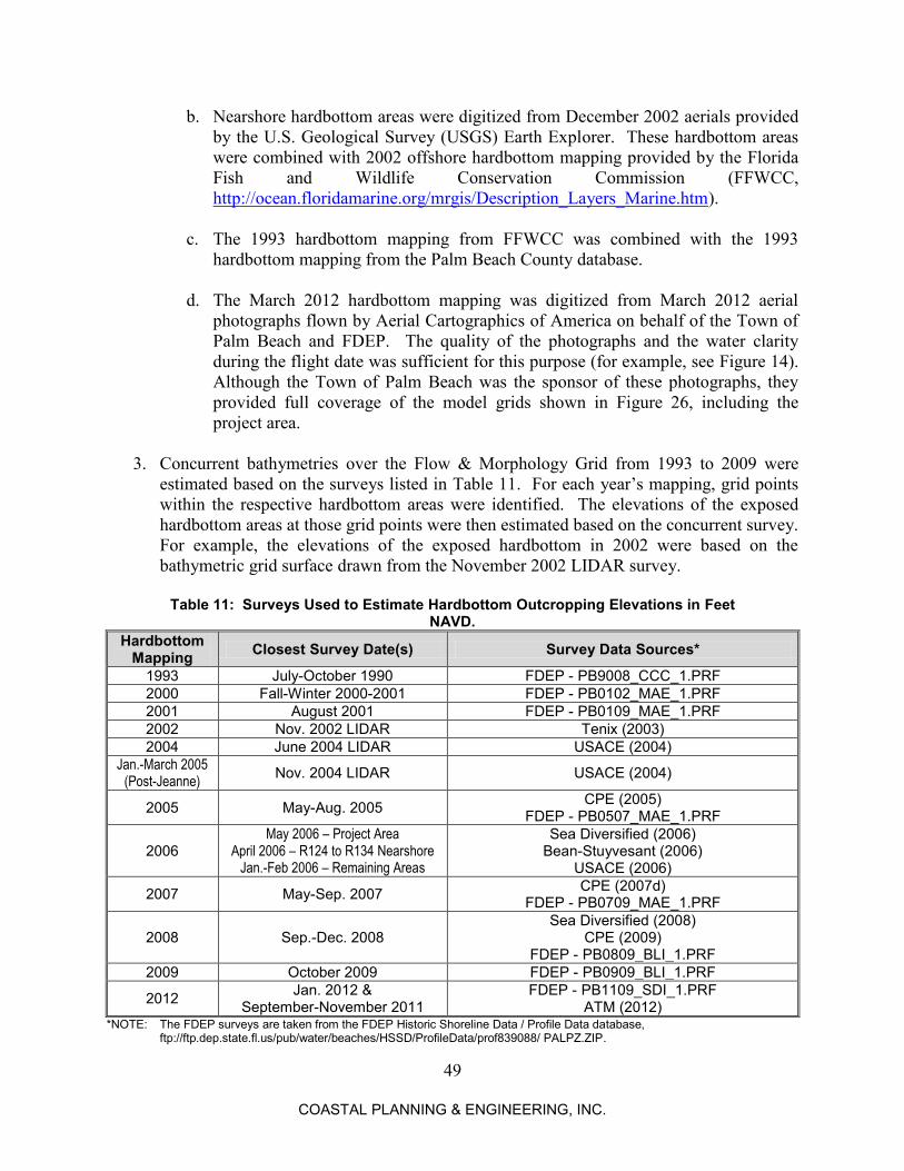
3. Concurrent bathymetries over the Flow & Morphology Grid from 1993 to 2009 were

estimated based on the surveys listed in Table 11. For each year’s mapping, grid points within the respective hardbottom areas were identified. The elevations of the exposed hardbottom areas at those grid points were then estimated based on the concurrent survey. For example, the elevations of the exposed hardbottom in 2002 were based on the bathymetric grid surface drawn from the November 2002 LIDAR survey.

Table 11: Surveys Used to Estimate Hardbottom Outcropping Elevations in Feet

NAVD. Hardbottom

Mapping Closest Survey Date(s) Survey Data Sources*

1993 July-October 1990 FDEP - PB9008_CCC_1.PRF 2000 Fall-Winter 2000-2001 FDEP - PB0102_MAE_1.PRF 2001 August 2001 FDEP - PB0109_MAE_1.PRF 2002 Nov. 2002 LIDAR Tenix (2003) 2004 June 2004 LIDAR USACE (2004)

Jan.-March 2005 (Post-Jeanne)

Nov. 2004 LIDAR USACE (2004)

2005 May-Aug. 2005 CPE (2005) FDEP - PB0507_MAE_1.PRF

2006 May 2006 – Project Area

April 2006 – R124 to R134 Nearshore Jan.-Feb 2006 – Remaining Areas

Sea Diversified (2006) Bean-Stuyvesant (2006)

USACE (2006)

2007 May-Sep. 2007 CPE (2007d) FDEP - PB0709_MAE_1.PRF

2008 Sep.-Dec. 2008 Sea Diversified (2008)

CPE (2009) FDEP - PB0809_BLI_1.PRF

2009 October 2009 FDEP - PB0909_BLI_1.PRF

2012 Jan. 2012 & September-November 2011

FDEP - PB1109_SDI_1.PRF ATM (2012)

*NOTE: The FDEP surveys are taken from the FDEP Historic Shoreline Data / Profile Data database, ftp://ftp.dep.state.fl.us/pub/water/beaches/HSSD/ProfileData/prof839088/ PALPZ.ZIP.

http://ocean.floridamarine.org/mrgis/Description_Layers_Marine.htm

50


4. In many areas, hardbottom outcroppings were visible in 2 or more sets of aerial

photographs. As a result, many grid points had several values associated with the hardbottom elevation, not just one. Thus, two different variations of the bedrock elevation were estimated in feet NAVD – one based on the average, estimated hardbottom elevations, and a second based on the highest hardbottom elevations. The second hardbottom elevation mapping based on the highest hardbottom elevations was eventually selected for further refinement during the model calibration process.

5. To further extend the bedrock surfaces developed above, two additional data sources were used:

a. The first reflector (seismic) mapping developed for the 2007 Town of Palm Beach borrow area investigation (Finkl, et al., 2008).

b. The minimum beach profile envelope on FDEP profiles R-124 to R-137. This was used to estimate erodible depth elevations where neither hardbottom information nor seismic data (Finkl, et al., 2008) was available. The minimum beach profile elevation was developed using the surveys in Table 3 and Table 11 and the Average Profile tool in Beach Morphology Analysis Package 2.0.

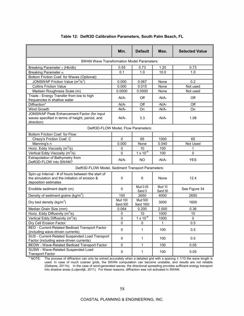
Using the methods and data sources listed above, several versions of the hardbottom/bedrock surface were developed as a calibration parameter, similar to CPE (2010). Further details regarding the variation of the hardbottom/bedrock surface are discussed in the next section. 4.2.7 Existing Structures The locations and elevations of the existing seawalls were verified based on the March 2012 aerial photograph, the Town of Lantana Seawall drawings by Taylor Engineering (2009), and the beach profile surveys listed in Table 3. In the SWAN model, the seawalls were treated as vertical walls with finite heights (“dams”) ranging from +12.4 to +18.7 feet NAVD. The overtopping coefficients = 1.8 and = 0.1 were equal to the recommended values for vertical walls (Deltares, 2011b). Reflection coefficients were assumed to be equal to 20%, similar to CPE (2010, 2011). In the Delft3D-FLOW model, the seawalls were treated as “thin-dams” that prevented flow from occurring through or over the structures regardless of water level. The representation of the Lake Worth Pier and the proposed structures under Alternatives B, D, and G is described in the next sections. 4.2.8 Model Calibration Sediment transport, erosion, and deposition parameters in the Delft3D-FLOW model were recalibrated based on the volumetric erosion rates between December 2008 and January 2012 (Figure 12). A total of 68 test simulations and calibration runs were conducted to identify the parameters best suited to simulating the general erosion pattern along the study area. Beginning with the model setup used in the 2011 alternatives report (CPE, 2011), the following model parameters were calibrated:

51


BED and SUS. These two parameters control the magnitude of the large-scale bedload

(BED) and suspended sediment (SUS) transport by currents, including longshore currents. These parameters have a default value of 1.0, but typically range from 0.5 to 1.5. In the original modeling study (CPE, 2010; 2011), the values of these parameters were BED = SUS = 0.6. The final values of these two parameters in this study were BED = SUS = 0.5.

BEDW and SUSW. These two parameters control the magnitude of the bedload (BEDW) and suspended sediment (SUSW) transport associated with the wave-driven orbital velocities. These parameters have a default value of 0, but usually range from 0 to 10% of BED and SUS. In the original modeling study (CPE, 2010, 2011), the values of these parameters were BEDW = SUSW = 0.125. The final values of these two parameters in this study were BEDW = SUSW = 0.05.

Grain Size. As noted in Section 2.3, the mean grain size for profiles R-124 to R-139 was

approximately 0.36 mm (1.49), based on samples collected by Palm Beach County (1993). However, this value represents an average of multiple samples. To examine the sensitivity of the model to grain size, a number of simulations were conducted using a mean grain size of 0.42 mm (1.26), which was based on the samples collected above −7.5 feet NAVD (−6 feet NGVD) only. Since this change did not affect the model results significantly, final value of the grain size was the value used in the original modeling study (CPE, 2010; 2011): 0.36 mm (1.49).

Lake Worth Pier Schematization. As shown in Figure 31, the Lake Worth Pier has a localized influence on the shoreline shape. Accordingly, several representations of the Lake Worth Pier in the model were examined:

Option 1. Negligible Influence: The pier was not used in the SWAN and Delft3D-FLOW models. In the original model study (CPE, 2010; 2011), the effects of the Lake Worth Pier were shown to be negligible.

Option 2. Permeable Structure: In the SWAN model, the pier was treated as a “sheet” of infinite height with transmission coefficients of 0.75, 0.85, and 0.93. In the Delft3D-FLOW model, the pier was treated as a “porous plate”, or a partially transparent structure that extends into the flow along one of the grid directions, with a thickness that is much smaller than the grid size in the direction normal to the porous plate. Unlike other types of structures in the Delft3D-FLOW model, mass and momentum can be exchanged through the porous plate. The porosity of the plate is controlled using a quadratic friction term, or “loss coefficient”, that is an input to the Delft3D-Flow model. Given permeabilities of 75 percent, 85 percent, and 93 percent, the equivalent loss factors for a 0.2 m/s (0.66 feet/second) longshore current would be 1.36, 0.65, and 0.28, respectively.

The final calibration run identified the Lake Worth Pier as a structure with a permeability of 85 percent for modeling purposes.

52


Phipps Ocean Park Borrow Area Representation. The Phipps Ocean Park Borrow Areas

were the most prominent bathymetric features near the project area (see Figure 26). Following the construction of the Phipps Ocean Park (Reach 7) Beach Restoration project in 2006, some slumping of the borrow areas occurred (see Figure 32).

Figure 31: January 24, 2009 Aerial Photograph of the Lake Worth Pier.

Figure 32: Typical Survey Profiles (R-133) across the Phipps Ocean Park South

Borrow Area.

NOTE SLUMPING ALONG THE SIDE OF THE BORROW AREA.

53


Figure 33: 2006 and 2008 Surveys near the Phipps Ocean Park Borrow Areas.

54


However, the coverage and resolution of the more recent surveys was not as good as the After-Dredging surveys performed by Bean-Stuyvesant (2006) (see Figure 33). To better resolve the bathymetry near the borrow areas, the initial condition was modified by using the 2006 After-Dredging surveys as the primary data sources offshore, instead of the 2008 surveys (see Figure 33). However, this change to the initial conditions did not improve the model’s results. Accordingly, the final calibration run used the more recent 2008 surveys as the initial bathymetry’s primary data sources (see Figure 26).

Activation of Wind Stress in the SWAN Model. In the present calibration effort, wind stress was activated in the majority of simulations, with a smaller number of simulations not including wind stress. As whole, the various test runs suggested that the model results could be improved by activating the default wind stress formulations in both SWAN and Delft3D-FLOW. Accordingly, the final calibration run included wind stress in both the SWAN and Delft3D-FLOW models.

Extrapolation of the Bathymetry from the Flow & Morphology Grid at the Northern and Southern Ends of the Local Wave Grid in the SWAN Model. To provide for a stable coupling between the SWAN and Delft3D-FLOW models, the Local Wave Grid is slightly longer than the Flow & Morphology Grid (see Figure 23). The SWAN model allows the bathymetry on the upcoast and downcoast edges of the Local Wave Grid to be:

1. Taken from the initial condition (see Figure 26), or 2. Extrapolated based on the updated bathymetry over the Flow & Morphology Grid.

In preliminary simulations, utilizing the first option led to unrealistic accretion near the north end of the Flow & Morphology Grid. Accordingly, the second option was utilized in subsequent simulations, including the final calibration run (see also CPE, 2010; 2011).

Erodible Sediment Depth. As noted earlier, several versions of the hardbottom/bedrock

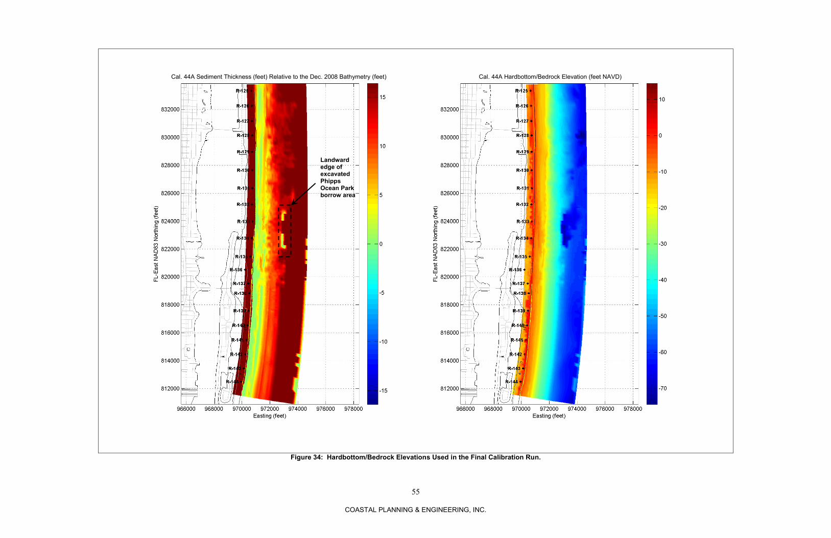
surface were developed as a calibration parameter. The hardbottom/bedrock surface was based on hardbottom outlines from various years, concurrent surveys (Table 11), seismic data (Finkl, et al., 2008), and the observed beach profile envelope. Nevertheless, due to the sampling of the survey and seismic data, the maximum elevations of the hardbottom/bedrock were strictly estimates. In some areas, it was necessary to eliminate small variations in the hardbottom/bedrock surface to improve the fit between the observed, 2008-2012 volume changes (see Figure 12) and the simulated volume changes. In addition, to moderate scour at the various seawalls, the erodible bed depth at the grid cells in front of them was set to 4.2 feet based on observed profile changes between December 2008 and January 2012, along with methods appearing in Fowler (1992). The final hardbottom/bedrock elevation based on the historical data review, the anomaly removal, and the scour limitation appears in Figure 34.

55


Figure 34: Hardbottom/Bedrock Elevations Used in the Final Calibration Run.

Cal. 44A Sediment Thickness (feet) Relative to the Dec. 2008 Bathymetry (feet) Cal. 44A Hardbottom/Bedrock Elevation (feet NAVD)

Landward edge of excavated Phipps Ocean Park borrow area

56


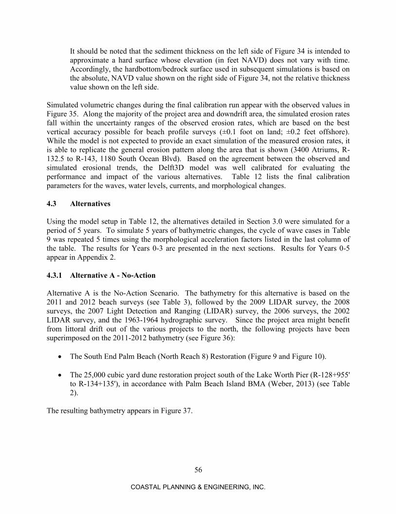
It should be noted that the sediment thickness on the left side of Figure 34 is intended to approximate a hard surface whose elevation (in feet NAVD) does not vary with time. Accordingly, the hardbottom/bedrock surface used in subsequent simulations is based on the absolute, NAVD value shown on the right side of Figure 34, not the relative thickness value shown on the left side.

Simulated volumetric changes during the final calibration run appear with the observed values in Figure 35. Along the majority of the project area and downdrift area, the simulated erosion rates fall within the uncertainty ranges of the observed erosion rates, which are based on the best vertical accuracy possible for beach profile surveys (±0.1 foot on land; ±0.2 feet offshore). While the model is not expected to provide an exact simulation of the measured erosion rates, it is able to replicate the general erosion pattern along the area that is shown (3400 Atriums, R-132.5 to R-143, 1180 South Ocean Blvd). Based on the agreement between the observed and simulated erosional trends, the Delft3D model was well calibrated for evaluating the performance and impact of the various alternatives. Table 12 lists the final calibration parameters for the waves, water levels, currents, and morphological changes. 4.3 Alternatives Using the model setup in Table 12, the alternatives detailed in Section 3.0 were simulated for a period of 5 years. To simulate 5 years of bathymetric changes, the cycle of wave cases in Table 9 was repeated 5 times using the morphological acceleration factors listed in the last column of the table. The results for Years 0-3 are presented in the next sections. Results for Years 0-5 appear in Appendix 2. 4.3.1 Alternative A - No-Action Alternative A is the No-Action Scenario. The bathymetry for this alternative is based on the 2011 and 2012 beach surveys (see Table 3), followed by the 2009 LIDAR survey, the 2008 surveys, the 2007 Light Detection and Ranging (LIDAR) survey, the 2006 surveys, the 2002 LIDAR survey, and the 1963-1964 hydrographic survey. Since the project area might benefit from littoral drift out of the various projects to the north, the following projects have been superimposed on the 2011-2012 bathymetry (see Figure 36):

The South End Palm Beach (North Reach 8) Restoration (Figure 9 and Figure 10).

The 25,000 cubic yard dune restoration project south of the Lake Worth Pier (R-128+955' to R-134+135'), in accordance with Palm Beach Island BMA (Weber, 2013) (see Table 2).

The resulting bathymetry appears in Figure 37.

57


Figure 35: Simulated Volume Changes during the Final Calibration Run.

58


Table 12: Delft3D Calibration Parameters, South Palm Beach, FL

Min. Default Max. Selected Value

SWAN Wave Transformation Model Parameters:

Breaking Parameter (Hb/db) 0.55 0.73 1.20 0.73 Breaking Parameter 0.1 1.0 10.0 1.0 Bottom Friction Coef. for Waves (Optional):

JONSWAP Friction Value (m2/s3) 0.000 0.067 None 0.2 Collins Friction Value 0.000 0.015 None Not used Madsen Roughness Scale (m) 0.0000 0.0500 None Not used

Triads - Energy Transfer from low to high frequencies in shallow water -N/A- Off -N/A- Off

Diffraction* -N/A- Off -N/A- Off Wind Growth -N/A- On -N/A- On JONSWAP Peak Enhancement Factor (for input waves specified in terms of height, period, and direction)

-N/A- 3.3 -N/A- 1.08

Delft3D-FLOW Model, Flow Parameters:

Bottom Friction Coef. for Flow: Chezy's Friction Coef. C 0 65 1000 65 Manning's n 0.000 None 0.040 Not Used

Horiz. Eddy Viscosity (m2/s) 0 10 100 1 Vertical Eddy Viscosity (m2/s) 0 1 x 10-6 100 0 Extrapolation of Bathymetry from Delft3D-FLOW into SWAN? -N/A- NO -N/A- YES

Delft3D-FLOW Model, Sediment Transport Parameters:

Spin-up Interval - # of hours between the start of the simulation and the initiation of erosion & deposition estimates

0 6 None 12.4

Erodible sediment depth (m) 0 Mud 0.05 Sand 5

Mud 10 Sand 50 See Figure 34

Density of sediment grains (kg/m3) 100 2650 4000 2650

Dry bed density (kg/m3) Mud 100 Sand 500

Mud 500 Sand 1600

3000 1600

Median Grain Size (mm) 0.064 0.200 2.000 0.36 Horiz. Eddy Diffusivity (m2/s) 0 10 1000 10 Vertical Eddy Diffusivity (m2/s) 0 1 x 10-6 1000 0 Dry Cell Erosion Factor 0 0 1 0.5 BED - Current-Related Bedload Transport Factor (including wave-driven currents) 0 1 100 0.5

SUS - Current-Related Suspended Load Transport Factor (including wave-driven currents) 0 1 100 0.5

BEDW - Wave-Related Bedload Transport Factor 0 1 100 0.05 SUSW - Wave-Related Suspended Load Transport Factor 0 1 100 0.05

* NOTE: The process of diffraction can only be solved accurately when a detailed grid with a spacing ≤ 1/10 the wave length is used. In case of much coarser grids, the SWAN computation can become unstable, and results are not reliable (Deltares, 2011b). In the case of wind-generated waves, the directional spreading provides sufficient energy transport into shadow areas (Luijendijk, 2011). For these reasons, diffraction was not activated in SWAN.

59


Figure 36: 2011-2012 and Alternative A Bathymetry Comparison.

60


Figure 37: Alternative A Flow & Morphology Grid Bathymetry.

61


The initial sediment thickness for Alternative A is based on the difference between the bathymetry shown in Figure 37 (left side) and the hardbottom/bedrock elevation shown in Figure 34 (right side). The resulting sediment thickness appears on the right side of Figure 37. It should be noted since the 2008 and 2011-2012 bathymetries are not the same, there are slight differences between the sediment thickness in Figure 34 (left side) and the sediment thickness in Figure 37 (right side). Model results given Alternative A appear in Appendix 2, Table 13, Table 14, and Figure 38 through Figure 40. Over the next 3 years, the model suggests that the project area (R-134+135' to R-138+551') could lose 81,000 c.y. These erosion rates are higher than the one shown in Table 4 (last column). However, the following must be noted:

The volume changes estimated by the model generally fall within the uncertainty ranges of the observed volume changes (see Figure 35).

Shoreline and volume changes along the project area and the adjacent beaches vary with respect to time, location, and magnitude (see Figure 11 and Figure 12).

Given these considerations, the estimated volume changes are reasonable. Within the project area, the model suggests that middle of the project area (R-135 to R-137) will experience the highest erosion rates under either wave climate. The observed volume changes between 2008 and 2012 indicated higher erosion along the northern half of the project area (see Table 4). However, an erosion hotspot centered further to the south is consistent with the 2004-2006 erosion rates (see Figure 11 and Figure 12) and the 2008 sidewalk collapse at Lantana Public Beach (see Figure 3). Low-tide shoreline changes appear in Figure 39. The model suggests that under the average Wave Climate A, the shoreline might be stable along a small section of the project area (R-135). However, most of the project area would experience shoreline retreat. At the Mayfair House (R-135.5), the model suggests that retreat could occur back to existing seawall. At other locations, the amount of dry beach width at Year 3 would be very small. Hardbottom coverage is detailed in Appendix 2 and summarized in Table 14. The values shown therein include hardbottom coverage only. CPE (2007a, pp. 44-45) notes that hardbottom exposure along the project area and the adjacent beaches varies widely over time, with hardbottom being covered and uncovered due to natural processes. The natural variability in hardbottom exposure is one of the primary reasons that Palm Beach County compiles hardbottom mapping information on a frequent basis (see Section 4.2.6 above).

62


Table 13: Volume Changes Based on the Delft3D Model, Years 0-3

Beach Volume Change, Entire Beach Profile, Pre-Construction versus Year 3 (cubic yards)

Beach Segment Length (feet) Alt. A Alt. B Alt. C Alt. D Alt. E Alt. F Alt. G

Reach 8 North 2,226 -21,500 -21,100 -21,200 -21,600 -21,400 -21,400 -21,600 R-125 to R-127+75' Lake Worth Public Beach 1,884 78,700 81,900 78,900 78,800 79,100 78,700 78,600 R-127+75' to R-128+955' Reach 8 South 6,542 -74,500 -49,200 -69,900 -67,200 -64,000 -70,600 -68,600 R-128+955' to R-134+135'

South Palm Beach Segment 2,679 -57,000 -11,200 -37,200 -8,200 17,600 -34,200 -8,300 R-134+135' to R-136+555' Lantana Segment 848 -20,400 -16,500 -12,600 -8,000 4,900 -12,100 -6,500 R-136+555' to R-137+395' Manalapan Segment 851 -3,600 400 6,100 2,400 10,900 6,100 1,900 R-137+395' to R-138+551' PROJECT AREA TOTAL 4,378 -81,000 -27,300 -43,700 -13,800 33,400 -40,200 -12,900 R-134+135' to R-138+551'

Downdrift 5,805 -6,900 -13,900 20,100 -6,600 21,600 14,400 -10,000 R-138+551' to R-144

NOTE: Negative (-) volume changes indicate erosion into pre-construction profile. Positive volume changes indicate accretion or remaining fill.

63


Table 14: Coverage of March 2012 Hardbottom at Year 3 Based on the Delft3D Model

(NOTE – This table does not include exposure of presently buried hardbottom, which occurs naturally and frequently along the project area)

Beach Hardbottom Coverage (acres)

Beach Segment Length (feet) Alt. A Alt. B Alt. C Alt. D Alt. E Alt. F Alt. G

Reach 8 North 2,226 0.0 0.0 0.0 0.0 0.0 0.0 0.0 R-125 to R-127+75' Lake Worth Public Beach 1,884 0.1 0.1 0.1 0.1 0.1 0.1 0.1 R-127+75' to R-128+955' Reach 8 South 6,542 2.1 2.4 2.2 2.2 2.3 2.2 2.2 R-128+955' to R-134+135' South Palm Beach Segment 2,679 0.3 0.4 0.3 0.5 0.5 0.3 0.6 R-134+135' to R-136+555' Lantana Segment 848 0.7 0.6 0.7 0.8 0.7 0.7 0.8 R-136+555' to R-137+395' Manalapan Segment 851 3.7 3.4 3.7 3.7 3.7 3.7 3.7 R-137+395' to R-138+551' PROJECT AREA TOTAL 4,378 4.8 4.5 4.7 5.1 4.9 4.7 5.1 R-134+135' to R-138+551' Downdrift 5,805 8.9 8.4 9.8 9.2 9.8 9.6 8.9 R-138+551' to R-144 TOTAL (R-125 to R-144) 20,834 15.9 15.4 16.7 16.5 17.0 16.6 16.3 PROJECT-INDUCED COVERAGE -N/A- -0.5 0.8 0.6 1.1 0.7 0.4 AT YEAR 3, R-125 to R-144

64


Figure 38: Volumes Changes Given Alternatives A and B.

65


Figure 39: Low-Tide Shoreline Changes, Alternatives A and B.

North Half of Project Area South Half of Project Area

66


Figure 40: Volume Changes versus Time.

Coverage of the present (March 30, 2012) hardbottom can be readily assessed based on the deposition that occurs in the model (> 0.2 feet) and the location of the present hardbottom (see Appendix 2). However, it is much more difficult to estimate the exposure of hardbottom that is presently buried, as the hardbottom/bedrock elevation in Figure 34 (right half) is an estimate. For these reasons, hardbottom exposure is not shown. Overall, hardbottom coverage values given the No-Action scenario (Table 14, 3rd column) are consistent with those of CPE (2011, pp. 22, 71). The degree of hardbottom coverage is consistent with the observed variability in exposed hardbottom along profiles R-134 and R-141 between March 1993 and May 2006 (see CPE, 2007a, pp. 44-45). 4.3.2 Alternative B - Original 2010 Recommended Plan Alternative B places 13 breakwaters and 75,000 cubic yards of fill material along the project area. The initial bathymetry for this alternative appears in Figure 41. Model results given Alternative B appear in Appendix 2, Table 13, Table 14, Figure 38 through Figure 40, and Figure 42. The model results suggest that under an average wave climate, the benefits associated with the project will be concentrated along the northern third of the project area and the quarter-mile segment updrift (R-133 to R-135) (see Figure 38 and Figure 39). Along these areas, erosion into the pre-construction shoreline will be prevented over the first 3 years.

67


Figure 41: Initial Bathymetry for Alternatives B, C, and D (excluding groins or

breakwaters).

68


Figure 42: Project-Induced Hardbottom Coverage versus Time.

Within the northern third of the project area, salients are shown to form along the shoreline. The model results also suggest that under an average wave climate, the breakwaters would have a minor impact on the downdrift segment between R-138+551' and R-139, along with the beaches facing the gaps between the structures (see Figure 38). Alternative B would bury approximately 1.56 acres of hardbottom during initial construction (see Table 5). This includes hardbottom covered directly by fill (1.11 acres) and the footprint of the structures (0.45 acres). However, the model suggests that after construction, the amount of additional hardbottom coverage that would occur would be less than the No Action scenario (Alternative A) due to the erosion and deposition patterns around the breakwaters (see Table 14 and Figure 42). 4.3.3 Alternative C - 75,000 Cubic Yards of Fill without Structures Alternative C features the same fill layout as Alternative B. However, breakwaters are not included. The initial bathymetry for this alternative appears in Figure 41. Model results given Alternative B appear in Appendix 2, Table 13, Table 14, Figure 40, and Figure 42 to Figure 44. In general, the model results show that there would be considerable spreading of fill given the construction of Alternative C (see Figure 43). In most areas, erosion into the pre-construction beach profile over the first 3 years would not be reduced substantially. The only exceptions might be the northern and southern ends of the project area (see Figure 43).

Project-Induced Hardbottom Coverage R-125 to R-144

69


Figure 43: Volume Changes Given Alternatives A & C.

70


Figure 44: Low-Tide Shoreline Changes, Alternatives A and C.


71


Alternative C would bury approximately 1.11 acres of hardbottom during initial construction (see Table 5). Model results suggest that project-induced hardbottom coverage could eventually increase over the 5 year post-construction period (see Figure 42). Overall, the model suggests that simply removing the breakwaters from the project’s design reduces the benefit of the project by at least half (see Table 13), while increasing the hardbottom impact (see Table 13 and Figure 42) due to sediment transport. Given these results, Alternative C does not offer any significant improvement over Alternative B or the County’s present shoreline management strategy of periodic dune fill placement (see Table 1). 4.3.4 Alternative D - 75,000 Cubic Yards of Fill with Short Groins Alternative D also features the same fill layout as Alternative B. However, the breakwaters are replaced by short groins as shown in Figure 16 and Figure 17. The initial bathymetry for this alternative appears in Figure 41. Model results given Alternative B appear in Appendix 2, Table 13, Table 14, Figure 40, Figure 42, Figure 45, Figure 46, and Figure 47. If Alternative D were constructed, erosion into the pre-construction shoreline would occur by Year 3. However, based on the model’s estimates, the amount of erosion would be 83 percent less than what would occur under Alternative A, and 68 percent less than what would occur under Alternative C (see Table 13 and Figure 47). Under an average wave climate, there could still be remaining beach fill at Year 3 along the northern and southern ends of the project area (see Figure 45, left half). The updrift benefits of the project would extend to roughly R-132. The model also suggests that the 3-year downdrift impact under an average wave climate would be negligible (see Table 13 and Figure 45). Alternative D would bury approximately 1.11 acres of hardbottom during initial construction (see Table 5). Model results suggest that project-induced hardbottom coverage would remain below this level under an average wave climate (see Figure 42 and Figure 45). Overall, the model suggests that replacing the breakwaters with groins increases the benefits of the project in terms of a more uniform beach response and decreases the downdrift, erosional impact (see Table 13 and Figure 47). Hardbottom coverage at construction would be less than Alternative B (see Table 5). Hardbottom coverage in the post-construction years would be comparable to or less than Alternative C (see Figure 42). Given these results, the addition of short groins to the project’s design is a feasible approach.

72


Figure 45: Volume Changes Given Alternatives A & D.

73


Figure 46: Low-Tide Shoreline Changes, Alternatives A and D.


74


Figure 47: Comparative Performance, Alternatives A, C, D, & F.

75


4.3.5 Alternative E - Fill Able to Last 3 Years without Any Structures The intent of Alternative E is to place enough fill to last 3 years without any coastal structures. The fill volume simulated was 160,600 cubic yards (Table 6). The initial bathymetry for Alternative E appears in Figure 48. Model results given Alternative E appear in Appendix 2, Table 13, Table 14, Figure 40, Figure 42, Figure 49, and Figure 50. Under an average wave climate, the volume placed under Alternative E would be able to last for 3 years (see Figure 49). Model results suggest that erosion into the pre-construction beach profile through Year 3 would be minimal. Except for the long taper near the southern end of the project area (R-137.5 to R-138+551'), the shoreline at Year 3 would be located near its pre-construction location (see Figure 50). The spreading of fill would generate an estimated benefit of 21,600 c.y downdrift (R-138+551' to R-144) and an updrift (R-128+955' to R-134+135') benefit on the order of 10,500 c.y. (see Table 13). Alternative E would bury 1.53 acres of hardbottom at construction (Table 6). After project construction, the model estimates that hardbottom impact could increase to 1.7 acres under an average wave climate (see Figure 42). Overall, the model suggests that under an average wave climate, Alternative E could be a viable solution, since the hardbottom impacts would be moderate (see Figure 42). Over the fill length as a whole, approximately 21 percent of the initial fill volume would be remaining at Year 3. 4.3.6 Alternative F –Fill Optimized to Minimize Hardbottom Impacts and Maximize

Project Life Alternative F places a fill volume similar to Alternative C, approximately 75,000 cy. However, to reduce hardbottom coverage and improve beach fill performance, fill is concentrated in the area of highest erosion near the middle of the project area. The initial bathymetry for this alternative appears in Figure 51. Model results given Alternative B appear in Appendix 2, Table 13, Table 14, Figure 40, Figure 42, Figure 47, Figure 52, and Figure 53. In general, the model results suggest that the performance of Alternative F would be similar to Alternative C, except for the following:

There would be an improvement in beach fill performance between Palm Beach Oceanfront Inn (R-135.5) and the Imperial House (R-136.5) (see Figure 47 and Table 13). While erosion into the pre-construction shoreline may occur along that area by Year 3, the degree of erosion would be less.

Project-induced hardbottom coverage would generally be less (see Table 13 and Figure 42).

76


Figure 48: Initial Bathymetry for Alternative E.

77


Figure 49: Volume Changes Given Alternatives A & E.

78


Figure 50: Low-Tide Shoreline Changes, Alternatives A and E.


79


Figure 51: Initial Bathymetry for Alternatives F & G (excluding groins).

80


Figure 52: Volume Changes Given Alternatives A & F.

81


Figure 53: Low-Tide Shoreline Changes, Alternatives A and F.


82


As a whole, the model results suggest that Alternative F offers slightly more benefits and somewhat less hardbottom impacts than Alternative C. However, the comparison of results between Alternatives C, D, and F suggests that adding groins (Alt. D) to a revised fill layout (Alt. F) could further improve project performance (see Figure 47). Based on that concept, an additional alternative was developed by combining the fill layout of Alternative F with the structural layout of Alternative D, resulting in Alternative G described below. 4.3.7 Alternative G - Fill Optimized to Minimize Hardbottom Impacts and Maximize

Project Life with Groins Alternative G included the optimized fill layout of Alternative F with the groin layout of Alternative D. The initial bathymetry for this alternative appears in Figure 51. Model results given in Alternative B appear in Appendix 2, Table 13, Table 14, Figure 40, Figure 42, Figure 54, Figure 55, and Figure 56. If Alternative G were constructed, erosion into the pre-construction shoreline would occur by Year 3 at some locations. However, under an average wave climate, the degree of erosion as estimated by the model would be manageable (see Figure 54), and it would be less than Alternatives D or F (see Figure 56). Based on the model’s estimates, the Year 3 shoreline north of the public beach (R-135+135’ to R-136+555’) would be located near its pre-construction location (see Figure 55). The updrift benefit of the project would extend to roughly R-132.5. Under an average wave climate, there would be a small downdrift impact (3,100 c.y., Table 13). However, since it would be spread over a long area (R-138+551’ to R-144), the effect in terms of fill density (c.y./foot) would be relatively small (see Figure 54). Alternative G would bury approximately 1.04 acres of hardbottom during initial construction (see Table 7). Under an average wave climate, the post-project hardbottom coverage would remain at or below this level based on the model’s estimates (see Figure 42). Overall the model results suggest that Alternative G achieves the best balance between beach fill performance and hardbottom impact. Although it does not prevent erosion into the pre-construction shoreline along the entire length of the project for 3 years, it reduces the average erosion to a manageable level under a typical wave climate (see Figure 54). Hardbottom impacts would be low to moderate (see Figure 42). Based the results of the model simulations and analytical analyses, the County’s objective to address erosion with a moderate sized project lasting 2 to 3 years, and the improved performance of the optimized fill distribution with groin stabilization, Alternative G is the recommended plan:

Approximately 75,000 cubic yards of sand in an optimized fill distribution. Seven groins extending from the existing seawalls to the post-construction water line.

83


Figure 54: Volume Changes Given Alternatives A & G.

84


Figure 55: Low-Tide Shoreline Changes, Alternatives A and G.


85


Figure 56: Comparative Performance, Alternatives A, D, F, & G.

86


5.0 RECOMMENDED PLAN - FILL OPTIMIZED TO MINIMIZE HARDBOTTOM IMPACTS AND MAXIMIZE PROJECT LIFE WITH GROINS (ALT. G)

Based on the model results in Section 4.3 above, Alternative G is the recommended plan. This alternative places approximately 75,000 cubic yards of material between the north end of South Palm Beach (R-134+135’) and the south end of the Ritz-Carlton hotel (R-135+551’) (see Table 7). The fill layout is optimized to place fill in the areas of greatest need while minimizing the degree of project-induced hardbottom coverage. Short groins are included along the middle of the project area to stabilize the fill material in the area of highest erosion (see Figure 16 and Figure 22). The length of each groin would be equal to the distance between the existing seawalls and the post-construction water line. 5.1 Long-Term Performance The long-term performance of the recommend plan (Alternative G) is summarized in Figure 57, Figure 58, Table 15, and Appendix 2. Under an average wave climate, there could be up to 12,900 c.y. of erosion into the pre-construction profile by Year 3, and 40,300 c.y. of erosion into the pre-construction profile by Year 5 (see Table 15). Remaining beach fill, if any, would be confined to some isolated sections near the north end of the fill area (Figure 57). North of R-136 (Thirty-Six Hundred Condominium), the 5 year shoreline would lie near its pre-construction location (Figure 58).

Table 15: Five Year Project Performance, Recommended Plan Alternative G - Fill Optimized to Minimize Hardbottom Impacts

and Maximize Project Life with Groins

Beach Volume Changes (cubic yards) versus Profile Lines Length Pre-Constr. Conditions, Entire Profile, Year 0 to Year …

(feet) 0 1 2 3 4 5 S. Palm Beach Segment 2,679 43,500 17,100 1,300 -8,300 -14,900 -20,400 R-134+135' to R-136+555' Lantana Segment 848 20,000 11,300 200 -6,500 -11,500 -15,500 R-136+555' to R-137+395' Manalapan Segment 851 8,500 11,900 6,300 1,900 -1,200 -4,400 R-137+395' to R-138+551' PROJECT AREA TOTAL 4,378 72,000 40,300 7,800 -12,900 -27,600 -40,300 R-134+135' to R-138+551' Downdrift 5,805 0 -16,100 -11,100 -10,000 -12,700 -17,000 R-138+551' to R-144

87


Figure 57: Performance of the Recommended Plan through Year 5.

88


Figure 58: Five Year Low-Tide Shoreline Changes Given the Recommended Plan.


89


Minor downdrift impacts would be likely under an average wave climate, beginning at Year 1 (see Table 15, Figure 57, and Appendix 2). Based on the results in Appendix 2, these would be roughly 5,400 c.y. over a 5 year period. However, on a fill density (c.y./foot) basis, the impact would be relatively small (see Figure 57). 5.2 Maintenance Requirements As shown in Table 15 and Figure 54, there may be some erosion into the pre-construction profile prior to Year 3 at some locations. If average wave conditions (Wave Climate A) prevail, the maintenance requirement at Year 3 would be on the order 84,900 cubic yards: approximately 75,000 c.y. per the original design (Table 7) plus the erosion that might occur into the pre-construction profile (see Table 15). This quantity is only an estimate as the required maintenance volume would depend on the actual wave climate, storm impacts and results of the post-construction physical monitoring of the project. 5.3 Hardbottom Impacts Hardbottom impacts are summarized in Table 16 and Figure 42. Impacts were based on the digitization of 2012 aerials (see section 4.2.6). Under an average wave climate (A), hardbottom impacts will be the highest at the time of initial construction. As the fill erodes, the impacts are expected to decrease as areas of hardbottom are re-exposed and the groins help retain sand with a moderate beach width.

Table 16: Five Year Project-Induced Hardbottom Coverage, Recommended Plan Alternative G - Fill Optimized to Minimize Hardbottom Impacts

and Maximize Project Life with Groins

Project-Induced Hardbottom Coverage (acres) Between Year 0 and Year …

0 1 2 3 4 5 1.04 0.3 0.4 0.4 0.4 0.4

5.4 Sea Turtle Nesting Benefits The recommended plan will increase the sandy beach width in front of the existing seawalls, which presently varies from 51 to 130 feet along the project area (Table 17, Table 18 and Appendix 3). Without a project in place, the sandy beach width will decrease. Based on the model results in Appendix 3, the 3 year decrease would average 33 feet under an average wave climate. The limited sand supply above the water line would likely restrict the degree of shoreline retreat after Year 3. The proposed groins are expected to be shore-perpendicular, low profile and short in the cross-shore dimension. These design features are intended to minimize impacts to nesting and hatchling sea-turtles, while stabilizing the beach to improve nesting habitat.

90


Table 17: Low-Tide Beach Width in Front of the Existing Seawalls

Recommended Plan Beach Width in Front of Seawalls (feet)*

Year Year Year Year Year Year 0 1 2 3 4 5 Recommended Plan (Alternative G)

Min. 85 44 34 41 32 40 Mean 124 91 77 79 76 79 Max. 173 144 127 140 126 140 No Action Scenario (Alternative A) Min. 51 30 28 29 28 29 Mean 92 63 56 58 56 59 Max. 130 98 97 94 96 100 Benefit in Terms of Width (refer to Appendix 3) Mean 32 28 21 21 19 20

* Represents distances from the seawalls to Mean Lower Low Water (-2.42 feet NAVD).

Table 18: Comparison of Existing (No-Action, Year 0) and Post-Project (Alternative G, Year 3) Average Beach Widths

Average Beach Width In Front of Seawalls

FDEP R- Monuments No Action (Year 0)

No Action (Year 3)

Alternative G (Year 3)

R-134+159' to R135 91 75 97 R-135 to R-136 73 50 78 R-136 to R-137 100 61 83 R-137 to R-138 107 48 59

R-138 to R-138+546' 91 43 49 * Equal to distances from the seawalls to Mean Lower Low Water (-2.42 feet NAVD).

Constructing the recommended plan would increase the beach width by an average of 32 feet and a maximum of 61 feet at the time of construction (see Table 17). After construction, the sandy beach width would decrease due to background erosion and the change in profile shape from a construction template to an equilibrium profile shape. Under an average wave climate, the typical sandy beach width in front of the seawalls would be 19 to 21 feet wider than the No Action scenario at Years 3 to 5 (see Table 17). The additional beach width gained by the project will offer benefits to nesting sea turtles. The survivability of the nest is a function of the distance predators and ants from the uplands or dunes have to travel to invade the nest. Wetterer et al. (2007) reported beach nourishment projects in the Southeastern United States reduced exposure attacks by 15 percent if the beach distance from the dune was at least 45 feet versus 26 feet. Approximately 12 percent of nests were invaded by ants 45 feet from the dune. In general, the FDEP does not recommend a minimum beach width;

91


however, guidance has been issued on turtle-friendly berm slopes that approximate the equilibrium profile to reduce the potential of scarping (FDEP, 2007). 5.6 Construction Costs Construction cost estimates associated with the recommended plan are presented in Table 19. Costs include $3,000,000 for beach fill and $700,000 for structures, $1,685,187 for associated costs including estimated mobilization, surveys, monitoring, mitigation and contingencies, for a total of $5,374,187. The unit cost of fill was based on recent dune projects completed in Lantana and South Palm Beach (2007, 2008 and 2009) and Hillsboro Beach. The unit costs of fill included mobilization and demobilization. Adjustments were made for inflation (Source: http://www.inflationdata.com/inflation/Inflation_Calculators/InflationCalculator.asp). The costs for the construction of the king pile and panel groins were based on recent cost estimates developed for a similar project being constructed at Big Hickory Island, Lee County, Florida. Table 7 suggests that the project will cover approximately 1.04 acres of hardbottom at construction based on hardbottom mapping digitized from March 2012 aerials. However, the actual mitigation and construction-phase monitoring requirements will be determined during the permitting process. As a first approximation, the cost estimate in Table 19 assumes that roughly 1.04 acres could be necessary depending on permitting requirements.

Table 19: Alternative G Estimated Construction Costs

Quantity Units Unit Cost Total Cost

Mobilization for Structures 1 $50,000 $50,000 King Pile and Panel Groins 7 Each $100,000 $700,000

Beach Fill (Trucking) 75,000 cy $40 $3,000,000 Surveys 1 $50,000 $50,000

Turbidity Monitoring 1 $5,000 $5,000 Turtle Nest Monitoring 2.5 months $16,250 $40,625

Hardbottom Mitigation 1.04 (approx.) acres $1,000,000 $1,040,000

Subtotal $4,885,625

Contingency (10%) $488,562 Total $5,374,187

Engineering, design, permitting and construction administration fees are not included in this cost estimate. 6.0 CONCLUSIONS Due to the effects of recent storms and long-term erosion, the shorelines along the Towns of South Palm Beach and Lantana are critically eroded. Although the long term erosional trend is moderate, erosion and shoreline retreats patterns can be highly variable due to the effects of storms, erosion waves, and nearshore hardbottom. To restore the shoreline to a moderate beach width, a shore protection project is being considered for the area between the northern end of South Palm Beach and the Ritz-Carlton hotel in Manalapan.

http://www.inflationdata.com/inflation/Inflation_Calculators/InflationCalculator.asp

92


To identify the most appropriate shore protection plan, the erosion rates between 2004 and the present were reviewed to assess the present erosion patterns. Seven alternatives were then formulated based on those erosion rates and previous studies of the project area. The Delft3D morphological model was recalibrated from previous studies based on more recent erosion patterns. The performance and impact of each alternative over a 3 year project life was then assessed using the calibrated model. The key findings of the engineering and numerical model study are:

A project including breakwaters is no longer considered a preferred means of addressing the project area’s erosion problem by Palm Beach County. However, the breakwater alternative was simulated with 75,000 cubic yards of fill for comparison with non-breakwater options. Benefits associated with breakwaters would be concentrated along the northern third of the project area and a 2,000 foot, updrift segment. Benefits along the rest of the project area would be low due to the effects of the breakwaters along the northern end.

Placing a uniform-width, 75,000 cubic yard beach fill without structures reduces the benefits of the project. It also results in hardbottom impacts beyond those expected to occur as direct impact at the time of construction. For this reason, a low-volume beach fill project without additional structures does not achieve the County’s objective for a project to last 2 to 3 years.

Adding short groins to a uniform-width and 75,000 cubic yard beach fill improves project performance with less impact to hardbottom than a similar project without structures.

Under an average wave climate, a larger fill project with 160,600 cubic yards would be able to prevent erosion into the existing beach for 3 years without new structures. However, the associated hardbottom impact would be greater. For this reason, a fill-only project with 160,600 cubic yards (or more) does not achieve the County’s objective for minimizing hardbottom impacts.

The strategic placement of 72,000 to 75,000 cubic yards based on the present erosion rates performs better than a similar-sized project with a uniform beach width. When short groins are added to the area of highest erosion, the combined fill and groin project becomes a viable means of offering short-term (3 year) shore protection under an average wave climate.

The recommend plan for the project area includes both sand fill and short groins strategically placed in conjunction to maximize the project life and minimize hardbottom coverage. Under a typical wave climate, the project is expected to last an average of 3 years, although minor erosion into the pre-construction beach profile may occur in some locations (< 10 c.y./foot). The hardbottom impact associated with this alternative is roughly 1.04 acres based on the March 2012 hardbottom mapping, which would occur primarily at construction. Changes in hardbottom exposure between the time of this analysis and the time of permitting and construction will result

93


in variations to these estimates and the mitigation that may be required by regulatory agencies. Excluding long-term physical and environmental monitoring, construction costs associated with the recommended plan are estimated to be $3,805,000 for beach fill and structures, $1,080,625 for hardbottom mitigation and turtle monitoring around the time of construction, and $488,562 for associated costs and contingencies, for a total cost estimate of $5,374,187. The results of this numerical modeling study should be used in conjunction with other coastal engineering assessments and prudent engineering judgment. Further engineering is recommended prior to implementation.

94


7.0 REFERENCES 3001, Inc. The Geospatial Company, 2008. Ground Control Survey Report, Ground Truth

Survey, for LIDAR Control, Professional Management and LiDAR Data Collection and Processing Services, Block 7, 3001, Inc. The Geospatial Company, Slidell, LA.

Aerial Cartographics of America, Inc., 2012. Town of Palm Beach Imagery (11706_2012),

Aerial Cartographics of America, Inc., Orlando, FL. Applied Technology & Management, 2009. 2010-2011 Dune Restoration, Town of Palm Beach

Florida, Applied Technology & Management, West Palm Beach, FL. Applied Technology & Management, 2012. Town of Palm Beach Town‐Wide 2011 Physical

Monitoring Report, Applied Technology & Management, West Palm Beach, FL. Bean-Stuyvesant, 2006. Town of Palm Beach, Phipps Ocean Park (Reach 7) Beach Nourishment

Project, After-Dredging Surveys, Bean-Stuyvesant, LLC, Belle Chasse, LA. Benedet, L., List, J.H., 2008. Evaluation of the Physical Process Controlling Beach Changes

Adjacent to Nearshore Dredge Pits, Coastal Engineering volume 55(12). 1224-1236. Campbell, Thomas J., 1992. The Beach Restoration Process in Florida, Short Course on

Principles and Applications of Beach Nourishment, University of Florida, Gainesville, Chapter 5.

Coastal Planning & Engineering, Inc., 2000. Palm Beach County, Florida, Shore Protection

Project, Ocean Ridge Segment, 1999 Monitoring Study, Coastal Planning & Engineering, Inc., Boca Raton.

Coastal Planning & Engineering, Inc., 2007a. Town of South Palm Beach/Town of Lantana

Erosion Control Study, Coastal Planning & Engineering, Inc., Boca Raton, FL. Coastal Planning & Engineering, Inc., 2007b. Town of Palm Beach, Florida Reach 8 Beach

Nourishment Project Engineering Design Development Report, Coastal Planning & Engineering, Inc., Boca Raton, FL.

Coastal Planning & Engineering, Inc., 2007c. Request for Additional Information (RAI #2)

Response, 0250572-001-JC, Palm Beach County, Town of Palm Beach, Reach 8 Beach Restoration, Coastal Planning & Engineering, Inc., Boca Raton, FL.

Coastal Planning & Engineering, Inc., 2007d. Coastal Construction Control Line Permit

Application for Town of Palm Beach Southern Dune Repair Project, Coastal Planning & Engineering, Inc., Boca Raton, FL.

95


Coastal Planning & Engineering, Inc., 2009. 2008 Town of Palm Beach Annual Monitoring, Topographic and Hydrographic Survey Report, Coastal Planning & Engineering, Inc., Boca Raton, FL.

Coastal Planning & Engineering, Inc., 2010. Central Palm Beach County Comprehensive

Erosion Control Project, Numerical Calibration of Wave Propagation and Morphology Changes, Coastal Planning & Engineering, Inc., Boca Raton, FL.

Coastal Planning & Engineering, Inc., 2011. Central Palm Beach County Comprehensive

Erosion Control Project Numerical Modeling of Shore Protection Alternatives, Coastal Planning & Engineering, Inc., Boca Raton, FL.

Coastal Systems International, Inc., 2012. Response to Request for Additional Information

(RAI) for the Proposed Truck Haul Beach Nourishment of Reach 8, Town of Palm Beach, Palm Beach County, Florida – JCP File No. 0250572-003, Coastal Systems International, Inc., West Palm Beach, FL.

Dean, Robert G., 1992. Engineering Design Principles: Part I – Design, Short Course on

Principles and Applications of Beach Nourishment, University of Florida, Gainesville, Chapter 2.

Deltares, 2011a. Delft3D-FLOW Simulation of Multi-Dimensional Hydrodynamic Flows and

Transport Phenomena, Including Sediments, User Manual, Part of Hydro-Morphodynamics, Deltares, Delft, the Netherlands.

Deltares, 2011b. Delft3D-WAVE, Simulation of Short-Crested Waves with SWAN, User

Manual, Part of Hydro-Morphodynamics, Deltares, Delft, the Netherlands. Finkl, C.W., Andrews, J.L., Forrest, B.M., Larenas, M.L., 2008. 2007 Geotechnical

Investigations to Identify Sand Resources Offshore of the Town of Palm Beach, Palm Beach County, Florida, Coastal Planning & Engineering, Inc., Boca Raton, FL.

Florida Department of Environmental Protection. 2007. Assessment of alternative construction

template for beach nourishment projects. Bureau of Beaches and Coastal Systems. Tallahassee, Florida.

Florida Department of Environmental Protection, 2013. Beaches and Coastal Systems Data,

Historic Shoreline Database, ftp://ftp.dep.state.fl.us/pub/water/beaches/HSSD/ProfileData. Fowler, J.E., 1993. Coastal Scour Problems and Methods for Prediction of Maximum Scour.

Technical Report CHL 93-8, U.S. Army Corps of Engineers Waterways Experiment Station, Coastal Engineering Research Center, Vicksburg, MS.

96


Leenknecht, D.A.; Szuwalski, A., and Sherlock A.R., 1992. Automated Coastal Engineering System Technical Reference. U.S. Army Corps of Engineers, Coastal Engineering Research Center, Vicksburg, MS.

Lesser G.R., Roelvink J.A., Van Kester J.A.T.M., Stelling G.S. 2004. Development and

Validation of a Three-Dimensional Morphological Model. Coastal Engineering 51 (2004), 883– 915.

Luijendijk, Arjen, 2011. E-mail to Christopher Day, Re: Input-Output problem(?) in Delft3D-

WAVE / SWAN - further info, November 25, 2011. National Oceanographic and Atmospheric Administration, 2003. Bench Mark Data Sheets, Lake

Worth Pier, FL, Station ID: 8722670, http://tidesandcurrents.noaa.gov/. National Oceanographic and Atmospheric Administration, 2006. GEODAS Software for

Windows, http://www.ngdc.noaa.gov/mgg/gdas/gx_announce.Html. National Oceanographic and Atmospheric Administration, 2013. WAVEWATCH III Model

Data Access, http://polar.ncep.noaa.gov/waves/download.shtml?. Palm Beach County, 1993. Environmental Assessment of Coastal Resources in Palm Beach,

Lake Worth, South Palm Beach, Lantana, and Manalapan, Palm Beach County, Florida, Palm Beach County, West Palm Beach, FL.

Palm Beach County, 2009. Approximate South Palm Beach/Lantana Project Timeline,

http://www.pbcgov.com/erm/coastal/shoreline/beach/pdf/South_Palm_Beach_Timeline_2009.pdf.

Palm Beach County, 2012. Palm Beach County Enterprise GIS Data Catalog, Sp_Hardbottom,

http://www.pbcgov.com/iss/itoperations/cwgis/GISdatasearch/ and ftp://pbcgis:sigcbp@ ftp.co.palm-beach.fl.us/ERM/SP_HARDBOTTOM.zip.

Sea Diversified Inc., 2006. Sea Diversified, Inc. Survey No. 05-784, May 22-26, 2006. Sea Diversified Inc., 2008. Sea Diversified, Inc. Survey No. 08-1344, December 2008. Taylor Engineering, 2009. Town of Lantana Phase II – Seawall Drawings, Taylor Engineering,

Jacksonville, FL. Tenix LADS Corporation, 2003. Data Acquisition and Processing Report, High Resolution

Hydrographic Survey of the Atlantic Coast of Dade and Palm Beach County, Florida Using Airborne Laser Technology, Tenix LADS Corporation, Biloxi, MS.

U.S. Army Corps of Engineers, 1991. Measurements for Lake Worth, FL,

http://sandbar.wes.army.mil/public_html/pmab2web/htdocs/florida/lakeworth/lakeworth.html.

97


U.S. Army Corps of Engineers, 2004. 2004 U.S. Army Corps of Engineers (USACE)

Topo/Bathy Lidar: Alabama, Florida, Mississippi and North Carolina, U.S. Army Corps of Engineers Joint Airborne LiDAR Bathymetry Technical Center of Expertise (JALBTCX), Mobile, AL, http://www.csc.noaa.gov/digitalcoast/data/coastallidar.

U.S. Army Corps of Engineers, 2006. USACE 2006 East Coast Topo/Bathy Mapping project,

U.S. Army Corps of Engineers Joint Airborne LiDAR Bathymetry Technical Center of Expertise (JALBTCX), Mobile, AL,

http://www.csc.noaa.gov/digitalcoast/data/coastallidar. U.S. Army Corps of Engineers, 2006. 2009 US Army Corps of Engineers (USACE) Joint

Airborne Lidar Bathymetry Technical Center of Expertise (JALBTCX) Lidar: East Coast of Florida, U.S. Army Corps of Engineers Joint Airborne LiDAR Bathymetry Technical Center of Expertise (JALBTCX), Mobile, AL, http://www.csc.noaa.gov/digitalcoast/data/coastallidar.

U.S. Geological Survey, 2002. Miami Dec-02 Aerial Photographs, USGS DOQs,

http://earthexplorer.usgs.gov/. Walton, Todd L., Chiu, T.Y., 1979. A Review of Analytical Solutions to Solve the Sand

Transport Equation and Some Simplified Solutions, Coastal Structures 79, American Society of Civil Engineers, New York.

Weber, Robert, 2013. E-mail to Thomas Pierro, Re: Town Projects, January 7, 2013. Wetterer, J.K., Wood, L.D., Johnson, C., Krahe, H., Fitchett, S. 2007. Predaceous ants, beach

replenishment, and nest placement by sea turtles. Entomological Society of America. Reference No. 0046-225X/07/1084Ð1091$04.00/0

P:\Palm Beach\South Palm Beach\142446 South Palm Beach Lantana

Revision\Report\South_Palm_Beach_2013_Alternatives_Modeling_draft_1.doc


APPENDIX 1

BEACH PROFILES USED TO ESTIMATE OBSERVED EROSION RATES


APPENDIX 2

DELFT3D MODEL RESULTS ASSUMING DECEMBER 2008 TO JANUARY 2012 WAVES

Notes:

1. This Appendix is provided in PDF format only.

2. The thin, magenta lines on the Erosion & Deposition and Impacts &

Benefits plots are the outlines of the March 2012 hardbottom mapping.


APPENDIX 3

DRY BEACH WIDTH IN FRONT OF THE EXISTING SEAWALLS GIVEN THE RECOMMENDED PLAN

Date post:	01-Apr-2018
Category:	Documents
Upload:	dokhanh
View:	219 times
Download:	4 times

CENTRAL PALM BEACH COUNTY COMPREHENSIVE...

Documents