9 Centralized Production of Hydrogen using a Coupled Water Electrolyzer-Solar Photovoltaic System James Mason 1 and Ken Zweibel 2 1 Hydrogen Research Institute, Farmingdale, NY 2 Primestar Solar Co., Longmont, CO 1 Introduction This study investigates the centralized production of hydrogen gas (H2) by electroly- sis of water using photovoltaic (PV) electricity. H2 can be used to power all modes of transportation. The logical first large-scale application of H2 is as a replacement fuel for light-duty vehicles, light commercial trucks, and buses. Since H2 is an expensive fuel compared to gasoline, consumer acceptance of H2 is contingent on its use in advanced fuel economy vehicles such as fuel cell vehicles (FCVs), which lowers the cost of H2 relative to the cost of gasoline used by conventional fuel economy ve- hicles. * The purpose of the study is to provide baseline projections of capital invest- ments, levelized H2 prices, and fuel cycle greenhouse gas (GHG) emissions of a centralized PV electrolytic H2 production and distribution system. This is important in order to evaluate the economic and environmental impacts of utilizing PV electro- lytic H2 as a fuel source. The use of PV electricity for electrolytic H2 production is a means of storing solar energy and overcoming its limitations as an intermittent power source. However, the intermittency of solar energy reduces the utilization capacity factor of electrolysis plants, which increases H2 production cost. The relevant question is whether the * Examples of advanced fuel economy vehicles are fuel cell vehicles (FCV), hybrid electric vehicles (HEV), and plug-in hybride electric vehicles. Fuel cell vehicles (FCVs) are on the verge of being ready for mass production. 2 FCVs are an attractive first application of H2 due to their enhanced fuel economy and superior driving per- formance. FCVs have powerful electric engines but do not require batteries to re- charge since the H2 running through the fuel cells produces electricity. The average fuel efficiency of FCVs is a factor of 2.2 greater than the fuel efficiency of conven- tional gasoline powered ICE vehicles.
Transcript
9
Centralized Production of Hydrogen using a Coupled Water Electrolyzer-Solar Photovoltaic System
James Mason1 and Ken Zweibel2
1Hydrogen Research Institute, Farmingdale, NY 2Primestar Solar Co., Longmont, CO
1 Introduction
This study investigates the centralized production of hydrogen gas (H2) by electroly-sis of water using photovoltaic (PV) electricity. H2 can be used to power all modes of transportation. The logical first large-scale application of H2 is as a replacement fuel for light-duty vehicles, light commercial trucks, and buses. Since H2 is an expensive fuel compared to gasoline, consumer acceptance of H2 is contingent on its use in advanced fuel economy vehicles such as fuel cell vehicles (FCVs), which lowers the cost of H2 relative to the cost of gasoline used by conventional fuel economy ve-hicles.* The purpose of the study is to provide baseline projections of capital invest-ments, levelized H2 prices, and fuel cycle greenhouse gas (GHG) emissions of a centralized PV electrolytic H2 production and distribution system. This is important in order to evaluate the economic and environmental impacts of utilizing PV electro-lytic H2 as a fuel source.
The use of PV electricity for electrolytic H2 production is a means of storing solar energy and overcoming its limitations as an intermittent power source. However, the intermittency of solar energy reduces the utilization capacity factor of electrolysis plants, which increases H2 production cost. The relevant question is whether the
* Examples of advanced fuel economy vehicles are fuel cell vehicles (FCV), hybrid electric vehicles (HEV), and plug-in hybride electric vehicles. Fuel cell vehicles (FCVs) are on the verge of being ready for mass production.2 FCVs are an attractive first application of H2 due to their enhanced fuel economy and superior driving per-formance. FCVs have powerful electric engines but do not require batteries to re-charge since the H2 running through the fuel cells produces electricity. The average fuel efficiency of FCVs is a factor of 2.2 greater than the fuel efficiency of conven-tional gasoline powered ICE vehicles.
272 James Mason and Ken Zweibel
production of electrolytic H2 using PV electricity is economically viable. This study attempts to provide insight into this question.
In all cases, the analysis draws on the perspective of the Terawatt Challenge for Thin Film PV in terms of PV costs, efficiencies, reliability, and progress towards these goals.1 The study assumes progress in PV technologies will occur. Then the important questions to be examined are: Does it matter? Will PV electricity be inex-pensive enough to make electrolytic H2 production practical? The study will answer these in the positive.
The organization of the study is as follows. In the first Section, a H2 production and distribution system is described. Secondly, capital and levelized H2 price esti-mates are investigated for each of the H2 system components. Thirdly, a life cycle evaluation of primary energy and GHG emissions in the H2 fuel cycle is performed. Sensitivity analyses are performed for the H2 price and the life cycle energy and GHG emissions estimates. The study concludes with a summary of findings and suggestions for future research.
2 Description of a PV Electrolytic H2 Production and Distribution System
The H2 production and distribution system analyzed in this study is scaled to a quan-tity of H2 for one-million FCVs. The components of the centralized H2 system are: a PV power plant; an electrolysis plant; a pipeline compression station; 621 miles (1,000 km) of long-distance pipeline with nine booster compressors sited at 60 mile intervals; four city gate distribution centers; and 1,000 local filling stations. The local distribution of H2 is by truck with metal hydride (MH) storage containers.* The H2 system is completed with the inclusion of regional underground H2 storage facilities designed to level seasonal variations in H2 supply and demand.
Each PV electrolysis plant produces 216-million kilograms of H2 per year. This H2 production level is sufficient to support the annual H2 consumption of one-million FCVs. In addition, the H2 production level takes into account 3% H2 distribution losses and the use of H2 to power pipeline booster compressors, city gate compres-sors, and city gate distribution trucks.† One-million FCVs consume 202-million kilograms of H2 per year, which is based on an average FCV fuel economy of 54.5
* A H2 system requires a H2 storage medium for delivery trucks, filling stations, and vehicles. The near-term choices for H2 storage are metal hydrides, compression at 10,000 psia, and liquid at extreme low temperatures. This study chooses to use a metal hydride H2 storage system as a baseline model because it is the least energy intensive means of storing H2. Collaborative DOE and industry metal hydride re-search goals are to achieve 6% H2/MH by weight storage ratio, a three minute re-charging time, thousands of recharging cycles, and low cost by 2010.
† The projection of 3%-H2 distribution losses is twice the natural gas distribution loss rate.10
Centralized Production of Hydrogen 273 mi/kg of H2 and an average annual travel distance of 11,000 miles over the range of all FCV light-duty vehicles and light commercial trucks.
The H2 from each PV electrolysis plant is transported to city gate distribution centers by pipeline. At the city gate distribution centers, the pipeline H2 is stored in metal hydride (MH) containers, which contain 2,000 kg of H2 at a H2/MH storage ratio of 6% by mass, and the MH containers are loaded onto tractor-trailer trucks and delivered to 1,000 local filling stations. At filling stations, the MH containers are stored in above-ground, cast-iron frames for fast replacement by tractor-trailer, con-tainer trucks. With an average FCV fill-up rate of 4.5 kg H2 per refueling stop, 330 FCVs can be refueled by one MH container with the MH container having a 75% of capacity discharge factor. The filling station MH containers are replaced on a two to four day cycle, and the empty MH containers are replaced and returned to the city gate distribution centers to be refilled with H2.
Cost estimates, performance parameters, and operating life of the central compo-nents of a PV electrolytic H2 system are listed in Table 1. All component cost esti-mates are based on an optimized manufacturing scale. PV cost estimates are from Zweibel1 and Keshner and Arya.3 The PV performance parameters of PV electrolysis plants are informed by studies of the solar hydrogen project at Neunburg vorm Wald, Germany.4,5 The performance parameters of electrolysers are from the collaborative study of large, grid-connected electrolyser plants by Norsk Hydro and Electricité de France.6* The cost estimates for H2 compressors are from Amos.7 The energy con-sumption of compressors used to transport and distribute H2 is estimated with an adiabatic compression energy formula provided by a Praxair representative8 and includes Redlich-Kwong H2 compressibility factors.9 Land costs, site preparation work, engineering and design, labor, and dismantling costs are factored into the component cost estimates.
The pipeline cost of $2.0-million per mile is based on an average natural gas pipeline cost of $1.5-million per mile, without compressor cost, with the addition of a 33% premium to take into account the cost for extra-secure pipe welds. More re-search is needed to accurately assess the capital costs of an integrated long-distance pipeline design for large regions such as the U.S., Europe, etc. The metal-hydride (MH) H2-storage container estimates are original to this study and are based on the assumption that some combination of metals such as magnesium, lithium, and boron
* The Cloumann et al.6 study of electrolytic H2 production is based on the use of grid-distributed electricity and the cost estimates include AC to DC rectifier/transformer units, which are not needed for electrolysis plants using dc electricity from PV power plants. The cost estimates also include compressors, H2 drying/purification units, and pumps for water and KOH circulation. The electrolysis performance efficiency of 61%, lower heat value, from the Cloumann et al. study is a global efficiency and includes the energy to compress H2 to a pressure of 33 bar, H2 losses in the dry-ing/purification phases, and the energy for pumping water and KOH. In contrast, this study models compression and pumping energy separately and assumes an electroly-sis efficiency of 64.2%. Separate PV installations are dedicated to provide electricity for H2 compression and water distillation and pumping. The assumed electrolyser efficiency of 64.2% is a conservative estimate and may prove to be closer to 66%.
274 James Mason and Ken Zweibel Table 1. Cost and performance assumptions for future PV electrolysis H2 systems.
Parameters Operating life (years)
A. PV power plant 1. PV area cost ($/m2) $60/m2 20, 30, 60
a. 2nd-generation PV area cost ($/m2) $50/m2 30 b. Freight charges @ $142/short ton $ 2/m2
3. PV balance of system (BOS) costs $50/m2 60 a. 2nd-generation BOS (only labor costs) $20/m2 30 b. Freight charges @ $100/short ton $ 2/m2
4. DC/DC converters $75/kWdc-in 30 5. PV system net efficiency (dc output per Wp installed) 85%
a. losses from wiring, ambient heat, module mismatch, etc.
– 11%
b. losses from dc/dc converters and coupling to electrolyzers
– 4%
6. PV system availability (included in PV-system efficiency)
99%
7. Average hours/day of peak insolation @ 271 W/m2 insolation
6.5 hours/day
8. O&M expenses including PV additions (% of capital) 1.0% 9. Land cost ($/acre) $1,000 10. Insurance (% of Capital) 0.0% 11. Property taxes (% of Capital) 0.5%
B. Electrolysis plant 1. Electrolysers (including dc-dc power conditioning) $ 425/kWdc-in 60 2. Electrolyser energy efficiency (H2 out/electricity in,
LHV) 64.2%
3. Electrolyser availability 98% 4. Electrolyser capacity factor 26.2% 5. Compressors (low pressure, water injected, screw type) $ 340/hp 30 a. compressor efficiency 70% b. energy to compress H2 from 14.7 psi to 116 psi 1.37 kWh/kg H2 6. Water system (collection, pumping, purification) $ 5,000,000 60 7. Administration, maintenance, and security buildings $10,000,000 60 8. O&M expenses (% of capital) 2.0% 9. Insurance (% of capital) 0.5%
10. Property taxes (% of capital) 0.5%
C. Other H2 system componentsa 1. Pipeline $2,000,000/mile 60 2. Pipeline compressors (reciprocating) $ 670/hp 40 3. Pipeline booster compressors (intervals) 60 miles 60 4. Metal-hydride (MH) H2 storage capital cost $ 30/kg MH 30 5. Insurance (% of capital) 0.5% 6. Property taxes (% of capital) 1.5%
aOther costs such as site preparation, engineering, legal, electrolyte replacement, etc. are included.
Centralized Production of Hydrogen 275 will be able to meet the assumed 6% H2 by weight storage capacity standard. The assumed MH cost of $30/kg is believed reasonable since magnesium production costs are < $4/kg, lithium production costs are < $2/kg, and boron production costs are < $1/kg.11 However, it needs to be emphasized that the MH cost and performance estimates are speculative and require additional analysis. The performance data for MH containers are from Chao et al.12
At present, the only PV technology clearly demonstrating the potential to meet the module cost ($60/m2) and minimum performance (10% PV module efficiency) projections of this study is thin film PV.1* Other combinations of module perfor-mance and cost (e.g., those of wafer silicon) are not as economical at the system level. Over time, additional PV technologies are expected to meet the PV cost and performance projections, and existing ones are expected to continue their cost reduc-tions and efficiency improvements. The baseline projections of this study assume a thirty-year PV module operating life. However, it is quite plausible, but not verifia-ble with present data, that the operating life of thin film PV will be sixty years with a 1%-annual degradation rate. Therefore, an analysis of H2 production costs with sixty year PV module operating life is performed and the results presented in the sensitivi-ty analysis section to provide a range in what can be realistically expected with fu-ture developments in thin film PV. A multi-MWp PV installation demonstrating the potential to achieve $50/m2 BOS costs, which includes land preparation, wiring conduit, electrical connection stations, PV system grounding, PV mounting hardware and installation, and union-scale labor, has been documented.13† The cost for dc/dc power conditioning equipment is categorized separately.
While a variety of electrolyser technologies are currently marketed, the type of electrolyser with a demonstrated ability to meet the cost and performance projections of this study are atmospheric, bi-polar, alkaline electrolysers.4 Alkaline electrolysers have a long track record for dependability, low-cost maintenance, and long operating life. The operating life of electrolysers is affected by the utilization rate.6 With a 26%
* It is assumed that 10% efficient thin film PV modules will be available for the near-term application of PV for large-scale electrolytic H2 production. At present, the best efficiency for a thin film PV module being produced at the > 50 MWp/year scale is 9.4%. While some thin film PV modules with efficiencies > 12% have been pro-duced on a small scale, there are numerous technical challenges in maintaining high efficiency levels while scaling-up PV manufacturing capacity. Therefore, it is as-sumed that 10% efficient PV modules will be available for the first large PV electro-lysis plants, and over time PV modules with higher efficiencies will become availa-ble. In addition, reaching module costs in the $50/m2 range requires further innovation and economies of scale.
† Tucson Electric Power at the Springerville PV plant has achieved $64/m2-BOS costs for MWp scale PV installations. With an increase to the multi-GWp scale in-stallation, it is reasonable to believe that a 25% reduction in BOS costs can be achieved through the mass manufacture and purchase of standardized BOS compo-nents and through efficiency gains in the allocation of labor/machinery for PV plant installation.
276 James Mason and Ken Zweibel
capacity factor of PV electrolysis plants, the electrolyser operating life is 60 years.14 At the low capacity factor of PV electrolysis plants, electrolyser maintenance will require nickel replating of electrolyser cells and electrodes only every twelve years rather than the normal seven year replating cycle with electrolyser capacity factors of 80% or greater. This reduction in maintenance cost almost entirely offsets the higher cost of low utilization factor electrolyser plants; an analysis that is expanded further in a later Section (see especially Fig. 3).
From the performance parameters in Table 1, the size of the electrolysis plant is 5.12 GWdc-in of electrolysers coupled to a 5.69 GWp PV power plant. An additional 0.15 GWp of PV is required for the electrolysis plant compressors, water pumps, and water distillation plant. The compressors and water pumps at the pipeline compres-sion station require another 0.13 GWp of PV. The cumulative size of the PV power plant is 5.97 GWp.
This study categorizes the costs of a PV power plant into:
1. PV modules; 2. dc/dc converters; and 3. balance of system (BOS) components, which include site preparation, PV
mounting frames, wiring, and labor.
The operating life of a PV power plant has two distinct generations. The first genera-tion is the initial construction of the PV power plant. While PV modules and dc/dc converters have a thirty-year operating life, many of the BOS components such as site preparation, mounting frames, underground wiring conduits, and PV array con-nection stations have a sixty-year operating life. With properly standardized module and BOS designs, capital investments in second generation PV power plants consists only in the costs of removing first generation PV modules and dc/dc converters and replacing them with new, second generation units without incurring the full range of BOS costs. Second generation BOS cost is reduced to labor for PV module mounting and inter-module wiring connection and is estimated at forty percent of first genera-tion BOS cost. This study also investigates the economic impacts of second genera-tion PV power plants with sixty-year PV module operating life.
The design of the PV power plant includes the annual addition of new PV to compensate for PV electricity output losses attributable to factors such as module soiling, PV module output degradation, and catastrophic PV module failures. The purpose of the PV additions is to maintain a constant level of electricity output to the electrolysers and compressors. Electricity losses from PV module soiling are as-sumed to be a constant 1.0% from year four to the end of the module operating life. The PV module degradation rate is assumed to be 1.0% per annum throughout the operating life of the PV modules. Catastrophic PV module failure, caused by factors such as manufacturing defects, glass stress fractures, and lightning strikes, is as-sumed to be 0.01% (1/10000) per annum. The financial accounting for the annual PV additions is treated as a normal O&M expense rather than as a capital investment.
To maximize the utilization capacity factor of PV electrolysis plants, it is as-sumed that PV electrolysis plants will be located at sites receiving high insolation (solar radiation) levels. Areas of the world with high insolation levels are presented in Fig. 1. This analysis assumes that PV electrolysis plants will be built at locations
Centralized Production of Hydrogen 277
Fig. 1. Areas of world with high average solar radiation levels (boxes). Copyright permission granted by Encyclopedia Britannica.
with a minimum average insolation level of 271 W/m2. This insolation level trans-lates into 6.5 hours of average daily peak PV electricity and electrolyser H2 produc-tion. PV installations are mounted at a fixed angle equaling the site’s latitude. The application of tracking systems for large field PV plants has not yet demonstrated cost effectiveness. The rows of the PV arrays are spaced to prevent cross-shading of modules when the sun is low in the sky from 9:00 am through 3:30 pm on December 21. The total area of the PV installation is approximately a factor of 3.0 greater than the area of the PV modules, which provides a small safety margin for installation variances.* The actual spacing of PV array rows to prevent module cross-shading will vary according to the site’s latitude.
The land area of a PV electrolysis plant to produce 216-million kg of H2/year is a function of insolation level, PV module efficiency, the spacing between the rows of the PV arrays, and the land required for electrolyser, compressor, administra-tion/maintenance/security buildings, water storage, water pumping and distillation facilities, PV for the pipeline compression station, and PV additions to compensate for PV degradation losses. A land area of 4 mi2 is allocated for electrolysers, com-pressors, administration buildings and water storage, pumping and distillation facili-ties. The total land area for the 5.97-GWp PV power plant is 94 mi2 for 10% efficient PV modules, 79 mi2 for 12% efficient PV modules, and 68 mi2 for 14% efficient PV modules. The land area includes the addition of 1.9 GWp of PV to compensate for PV output degradation losses. While this is a substantial land area, it is not prohibi-
* The row spacing estimate is based on 33o latitude and a sun altitude of 14.9o above the horizon at 9:00 am. The actual row spacing is a factor of 2.88 greater than the length of the modules and 0.12 is added as a safety buffer.
278 James Mason and Ken Zweibel
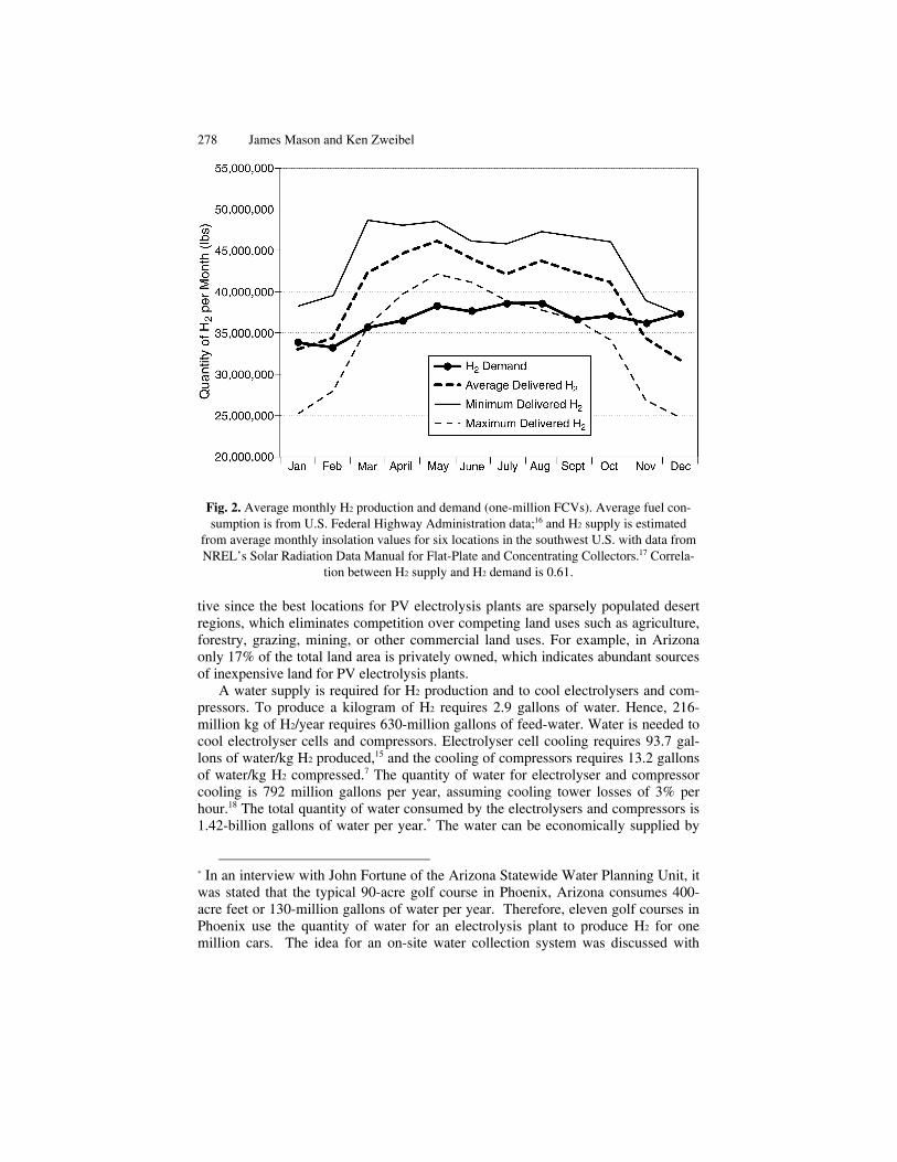
Fig. 2. Average monthly H2 production and demand (one-million FCVs). Average fuel con-sumption is from U.S. Federal Highway Administration data;16 and H2 supply is estimated
from average monthly insolation values for six locations in the southwest U.S. with data from NREL’s Solar Radiation Data Manual for Flat-Plate and Concentrating Collectors.17 Correla-
tion between H2 supply and H2 demand is 0.61.
tive since the best locations for PV electrolysis plants are sparsely populated desert regions, which eliminates competition over competing land uses such as agriculture, forestry, grazing, mining, or other commercial land uses. For example, in Arizona only 17% of the total land area is privately owned, which indicates abundant sources of inexpensive land for PV electrolysis plants.
A water supply is required for H2 production and to cool electrolysers and com-pressors. To produce a kilogram of H2 requires 2.9 gallons of water. Hence, 216-million kg of H2/year requires 630-million gallons of feed-water. Water is needed to cool electrolyser cells and compressors. Electrolyser cell cooling requires 93.7 gal-lons of water/kg H2 produced,15 and the cooling of compressors requires 13.2 gallons of water/kg H2 compressed.7 The quantity of water for electrolyser and compressor cooling is 792 million gallons per year, assuming cooling tower losses of 3% per hour.18 The total quantity of water consumed by the electrolysers and compressors is 1.42-billion gallons of water per year.* The water can be economically supplied by
* In an interview with John Fortune of the Arizona Statewide Water Planning Unit, it was stated that the typical 90-acre golf course in Phoenix, Arizona consumes 400-acre feet or 130-million gallons of water per year. Therefore, eleven golf courses in Phoenix use the quantity of water for an electrolysis plant to produce H2 for one million cars. The idea for an on-site water collection system was discussed with
Centralized Production of Hydrogen 279 either on-site water collection and storage systems or imported by train or truck. The quantity of water is one inch of rainfall over the PV plant area. Under no condition should the PV electrolysis plant draw water from underground aquifers, lakes, or rivers.
The effects of seasonal variation in insolation levels on seasonal H2 supply/demand balances are presented in Fig. 2. The seasonal H2 production profile is well suited to meet seasonal H2 demand. The positive 0.61 correlation between monthly H2 production levels by PV electrolysis plants and monthly H2 demand reduces the required capacity of underground storage facilities.
The high H2 output in the spring months insures that the underground H2 storage facilities will have sufficient H2 capacity to meet summer peak demand. The mini-mum and maximum H2 production curves are based on the minimum and maximum insolation levels recorded for each month over a ten year record of insolation levels for six locations in the southwest U.S. from west Texas to east California. The curves for the minimum and maximum insolation levels represent the extreme case where all locations receive the historical minimum or maximum insolation level in the same month. It is highly unlikely that minimum or maximum insolation levels will occur in the same month at each of the locations distributed over such a large area. But the minimum H2 production level estimate is useful as a yardstick in assessing the quan-tity of H2 that should be stored in underground storage facilities as reserves to insure adequate H2 supplies in the event of a variety of contingencies that could disrupt H2 supply.
The pipeline transport of H2 requires compression. The electrolysis plant uses low-pressure, water injected, screw-type compressors to compress H2 from 1.02 bar to 8.0 bar to transport the H2 a short distance (~ 10 miles) to a pipeline compression station. The energy to compress H2 from 1.02 bar to 8.0 bar is 1.37 kWh/kg of H2. There is no need for H2 storage at the electrolysis plant. At the pipeline compression station, the H2 is compressed from 8.0 bar to a pipeline pressure of 69.0 bar by high-pressure reciprocating compressors. The energy to compress H2 from 8.0 bar to a pipeline pressure of 69.0 bar is 1.17 kWh/kg of H2. PV electricity is used to power the compressors and water pumps at the compression station.
3 Capital Investment and Levelized Price Estimates
Capital cost estimates for the H2 system are presented in Table 2. The PV power plant is the largest capital component. With 10% efficient PV modules, the PV pow-er plant accounts for 59% of total capital investments. With cost reductions achieved by PV module efficiency gains, the proportion of capital for 14% efficient PV mod-ules is reduced to 51%. The second largest capital investment component is the elec-trolysis plant. The electrolysis plant accounts for 18–22% of total capital for
Fortune. Fortune stated that Arizona is willing to work closely with companies and developers who build rain-runoff water collection and storage systems, and he stated that he believes an on-site rain-runoff water collection and storage system for elec-trolysis plants is feasible.
280 James Mason and Ken Zweibel
Table 2. Capital estimates for future PV electrolytic H2 systemsa (scaled to serve 1-million fuel cell vehicles).
1. PV power plant (5.972-GWp) A. PV cost 3,702,390,460 3,085,325,383 2,644,564,614 B. PV BOS cost 3,105,230,708 2,587,692,257 2,218,021,935 C. DC/DC power conditioning 429,955,021 429,955,021 429,955,021
2. Electrolysis plant (5.121-GWp) A. Electrolyser cost 2,176,288,879 2,176,288,879 2,176,288,879 B. Compressor cost 60,738,708 60,738,708 60,738,708 C. Water system cost 5,000,000 5,000,000 5,000,000 D. Administration buildings 10,000,000 10,000,000 10,000,000
4. City Gate Distribution Centers (4) A. City Gate Distribution Centers 26,500,000 26,500,000 26,500,000 B. City Gate Compressors 28,957,500 28,957,500 28,957,500 C. H2 Delivery Trucks 22,500,000 22,500,000 22,500,000 D. MH Containers 1,300,000,000 1,300,000,000 1,300,000,000
5. Refueling Stations (1,000) A. MH Container Stands 10,000,000 10,000,000 10,000,000 B. Filling Station Compressors 12,300,000 12,300,000 12,300,000 C. Filling Station Dispensers 30,000,000 30,000,000 30,000,000
Subtotal 52,300,000 52,300,000 52,300,000 Total Capital Costs of H2 System 12,367,382,820 11,232,480,149 10,422,049,057
the 10% and 14% efficient PV module cases respectively. The pipeline system and city gate distribution centers are the next largest capital components and account for 12% and 11% of total capital respectively. The metal hydride H2 storage containers are 94% of the capital investments for the city gate distribution centers. The remain-ing capital component is the local filling stations, which is less than 1% of total capi-tal investments.
Hydrogen production and PV electricity prices are presented in terms of levelized prices. Levelized price is the constant revenue stream that recovers all capital in-vestments (equity and debt) at the required rates of return and covers annual O&M expenses, insurance, property tax, and income taxes over the assigned capital recov-
Centralized Production of Hydrogen 281 ery period. The levelized H2 price estimates are based on a thirty-year capital recov-ery period and a 6.0% discount rate.
The discount rate is a weighted average cost of capital (WACC) and takes into account the capital structure of firms, cost of equity and debt, and income taxes. The capital structure of firms is assumed to be 30% equity and 70% debt. The cost of equity capital is 10%, the cost of debt is 7%, and the effective income tax rate is 39%. The debt instrument is assumed to be a 20-year, 7% coupon bond. The calcula-tion of the discount rate is
The levelized prices of PV electricity and H2 are derived by net present value cash flow analysis. The net present value cash flow method is described in Appendix A.1. A straight-line, ten-year depreciation schedule is applied with an annual depre-ciation rate of 9% of capital. The levelized PV electricity and H2 prices are derived by choosing PV electricity and H2 prices to generate a revenue level that results in a cumulative, net cash flow stream with a $0-net present value over the thirty-year capital recovery period. The annual net cash flow streams are discounted at the present value of the 6%-discount rate. Investment funds are allocated in year 1; con-struction occurs in year 2; and H2 cash flow begins in year 3. The modular design of PV electrolysis plants and H2 distribution systems enables the rapid initiation of H2 marketing and cash flow.
The levelized H2 and PV electricity price estimates are presented in Table 3. The PV electrolysis plant dominates H2 production cost. The PV electrolysis plant com-ponent of the levelized H2 pump price ranges from $3.75–$4.67 per kg H2 contingent on PV module efficiency and PV area cost. The total levelized H2 pump price ranges from $5.53–$6.48 per kg H2.* The levelized H2 pump price estimates do not include fuel use taxes. In the U.S., fuel use taxes typically range from $0.40–0.50/gallon of gasoline, which translates into a H2 pump price of $6.52–$7.47/kg with tax.
While a kilogram of H2 is a gallon of gasoline equivalent in terms of energy con-tent, it is not a gallon of gasoline equivalent in terms of fuel cost when the H2 is consumed by fuel cell vehicles (FCVs). The fuel efficiency of FCVs with their po-werful electric engines is much greater than the fuel efficiency of internal combus-tion engines (ICE) vehicles. The average fuel economy of FCVs is 54.5-mi/kg H2, whereas the average fuel economy of conventional ICE vehicles is 23.5-mi/gal gaso-line. When H2 is used to power FCVs, the gallon of gasoline equivalent price is $2.81–$3.22, which is comparable to high-end 2005–2006-U.S. gasoline prices.
The PV electrolysis plant cost components account for 68–72% of the levelized H2 pump price. This can be seen by comparing the H2 production costs listed in Ta-ble 3.B.1 to the levelized H2 pump prices listed in Table 3.C. Of the PV electrolysis plant cost factors, the price of PV electricity is the dominant factor on H2 production costs. The large effect of PV module efficiency on H2 production costs is apparent by
* In terms of work energy, the energy content of a kilogram of H2 is approximately equivalent to the energy content of a gallon of gasoline. Therefore, a kilogram of H2 is considered to be a gallon of gasoline equivalent (gge) metric.
282 James Mason and Ken Zweibel
Table 3. Financial overview of a PV electrolytic H2 system (scaled to serve 1-million fuel cell vehicles).
Electricity price
($/kWh)
Capital investments (million $)
Annual revenues
(million $)
PV additions expense
(million $)
O&M expense
(million $)
A. PV power plant with 10% Efficient PV 0.064 7,238 769 72 5 with 12% Efficient PV 0.054 6,103 649 60 5 with 14% Efficient PV 0.047 5,293 562 52 5
H2 price ($/kg)
Capital investments (million $)
Annual revenues
(million $)
Electricity expense
(million $)
O&M expense
(million $)
B. H2 production and distribution 1. Electrolysis Plant 2,252 56
with 10% Efficient PV 4.67 1,013 753 with 12% Efficient PV 4.12 894 635 with 14% Efficient PV 3.75 813 553
2. Pipeline Transport 1,448 54 with 10% Efficient PV 0.97 104 16 with 12% Efficient PV 0.97 104 13 with 14% Efficient PV 0.95 104 12
3. City Gate Distribution Centers (4) 0.77 1,378 162 0 39
4. Local Filling Stations (1000) 0.07 52 11 6 1
C. Totals with 10% Efficient PV 6.48 12,367 2,059 775 144 with 12% Efficient PV 5.93 11,232 1,820 654 144 with 14% Efficient PV 5.53 10,422 1,652 571 144
reviewing Table 3. An increase in PV module efficiency, from 10% to 14%, lowers H2 production costs by 20% and the levelized H2 pump price by 15%.
The large effect of electricity price on H2 production costs is readily apparent in Fig. 3, which breaks down H2 production cost by electrolysis plant cost factors. The cost of electricity accounts for greater than 80% of H2 production costs across the range of electrolyser capacity factors. One of the criticisms to the application of PV electricity to electrolytic H2 production is its intermittent supply, which lowers the utilization capacity factor of electrolysers and increases H2 production cost. The low electrolyser capacity factor cost penalty is evaluated in Fig. 3. Over the 25–95% range in electrolyser capacity factors presented in Fig. 3, the H2 production cost of an electrolysis plant with a 25% capacity factor is approximately 11% higher than the H2 production cost of an electrolysis plant with a 95% capacity factor.* In other
*From Fig. 3, it is obvious that the relationship between electrolyser cost and H2 production cost across a 25–95% capacity factor range is non-linear. In this case, the appropriate method to evaluate the effect of electrolyser cost on H2 production cost
Centralized Production of Hydrogen 283
Fig. 3. Levelized H2 production price as a function of electrolyser capacity factor.
words, the utilization rate of electrolysers is not a particularly important issue in terms of H2 production cost because of the impact of offsetting factors such as elec-trolyser O&M expense and electrolyser operating life.
The critical element affecting the production cost of electrolytic H2, over the range of electrolyser capacity factors, is electricity cost. While the 11%-H2 cost pe-nalty for the low electrolyser capacity factor from the use of PV electricity is signifi-cant, it is hardly prohibitive. In conclusion, based on the assumed progress in PV cost reduction, PV electricity can be an economically viable source of electricity for electrolytic H2 production.
4 Sensitivity Analysis: H2 Production and PV Electricity Prices
Sensitivity analyses are performed to evaluate the effect of changes in cost factor values on H2 production and PV electricity prices. The cost factors for H2 production are: PV electricity; electrolysers; electrolyser operating capacity factor; electrolyser efficiency (in terms of converting electricity energy input into H2 energy output); electrolyser O&M expense; and the discount rate. The cost factors for PV electricity
across the range of electrolyser capacity factors is a log-linear regression model. A log-linear regression model transforms the non-linear dependent variable, H2 produc-tion cost, into a linear variable by using its natural logarithm value. The log-linear regression result indicates that a 1% increase in electrolyser capacity factor reduces H2 production cost by 0.16%. Hence, a 70% increase in electrolyser capacity factor decreases H2 production cost by only 11.2% (0.16% x 70).
284 James Mason and Ken Zweibel
production are: PV modules; PV BOS; PV module efficiency (rated PV module conversion of sunlight into dc electricity under standard test conditions); average insolation level; and the discount rate. The assigned range of values for the electroly-sis plant and PV power plant cost factors are presented in Table 4. The mean value for each of the cost factors is the value used to generate the baseline H2 production and PV electricity price estimates reported in this study.
The sensitivity estimates for the effect of changes in cost factor values on leve-lized H2 production and PV electricity prices are estimated by the least-squares, linear regression method. The regression results provide an estimate of the effect of unit changes in cost factor values on H2 production and PV electricity prices. The sensitivity results are presented in Table 5, Fig. 4, and Fig. 5.
The appropriate unit change for each of the cost factors are presented in paren-thesis in Table 5. The results in Table 5 report the increase/decrease (+/–) in H2 pro-duction price (¢/kg) and in PV electricity price (¢/kWh) caused by a unit increase in cost factor values. The interpretation of the effect of a unit decrease in cost factor values requires changing the sign (+/–) of the estimated change in H2 production and PV electricity price. Also, note that the regression sensitivity results can be applied to component values outside the range of component values presented in Table 4.
The sensitivity results reported in Table 5 for H2 production price are as follows. A $0.01/kWh increase in electricity cost causes H2 production price to increase by $0.55/kg. A $25 increase in electrolyser cost ($/kWdc-in) causes H2 production price to increase by $0.04/kg. A 1% increase in electrolyser capacity factor causes H2 pro-duction price to decrease by $0.02/kg. A 1% increase in electrolyser efficiency (LHV) causes H2 production price to decrease by $0.04/kg. A 1% increase in electro-lysis plant O&M expenses, which includes water system and compressors, causes H2 production price to increase by $0.09/kg.* A 1% increase in the discount rate causes H2 production price to increase by $0.09/kg. To evaluate the effect of a decrease in cost factor values simply reverse the sign, positive or negative, for the change in H2 production price.
The sensitivity results for PV electricity prices are as follows. A $5/m2 increase in the area cost of PV modules causes PV electricity price to increase by $0.002/kWh. A $5/m2 increase in the area BOS cost causes PV electricity price to increase by $0.002/kWh. A 1% increase in PV module efficiency causes PV electric-ity price to decrease by $0.004/kWh. A 42 W/m2 increase in the average insolation level, which represents a 1.0 hour increase in the average daily peak insolation
* The linear regression estimates that evaluate the effect of electrolyser capacity factor on H2 production cost need to be qualified. As previously noted in the foot-note on page 275, the relationship between electrolyser cost and H2 production cost over the full 25–95% range of capacity factors is non-linear. However, over the 25–29% range of electrolyser capacity factors applicable for PV power plants the rela-tionship is approximately linear. Also, it should be noted that over the 25–29% capacity factor range the effect of change in capacity factor is greater than over the 25–95% range because the curve is steeper (greater change) at the low-end of the capacity factor range as can be seen in Fig. 3.
Centralized Production of Hydrogen 285
Table 4. Descriptive statistics: value ranges to generate regression estimates.
B. Effect of change in H2 distribution values - Pipeline (per $250,000/mile) 7.7 - Metal hydride containers (per $5/kg) 9.9
C. Effect of Change in PV Power Plant Values on Electricity Price - PV Cost $/m2 (per $5/m2) 0.2 - BOS Cost $/m2 (per $5/m2) 0.2 - PV Efficiency (per 1.0 %) – 0.4 - Insolation Level (per 0.5 average peak hours/day) – 0.4 - Discount Rate (per 0.5 %) 0.2
286 James Mason and Ken Zweibel
Fig. 4. Effect of change in electrolysis plant values on levelized H2 production cost.
Fig. 5. Effect of change in PV plant values on levelized PV electricity price.
Centralized Production of Hydrogen 287 level, causes PV electricity price to decrease by $0.008/kWh. A 1% increase in the discount rate causes PV electricity price to increase by $0.004/kWh. And as pre-viously stated, to evaluate the effect of a decrease in cost factor values simply re-verse the sign, positive or negative, for the change in PV electricity price.
The slopes of the lines in Fig. 4 are a good demonstration of the relative impact of change in the cost factor values on H2 production price. Consistent with previous findings, the sensitivity results clearly indicate the dominance of electricity cost on electrolytic H2 production price. In decreasing order of effect are electrolyser effi-ciency, electrolyser O&M, and electrolyser cost. A degree of uncertainty exists re-garding the cost of electrolysers. At present, large electrolysers are manufactured in small numbers and include ac/dc power conditioning equipment. It is possible that the cost of mass produced electrolysers (thousands of units per year) without power conditioning equipment will be lower than the $425/kWdc-in cost estimate.
For PV electricity price, PV module efficiency and insolation level have the greatest impact. The variables having the next largest effect on PV electricity price are PV area cost and BOS area cost. A PV electricity price decrease associated with an increase in PV efficiency is contingent on holding area related PV manufacturing cost constant while achieving PV module efficiency gains.
Due to the large impact of insolation levels on PV electricity prices, a map of in-solation levels for the U.S. is presented in Fig. 6. The map clearly indicates that the U.S. is endowed with a large land area with high insolation levels, i.e., insolation levels ≥ 271 W/m2.
It is highly probable that PV module efficiencies will increase above the near-term 10% module efficiency, which implies that over time H2 production price will decrease. A decrease in BOS cost is contingent on scale economies achieved through the bulk purchase of standardized BOS components and strict attention to the man-agement of labor costs, i.e., design of tasks to maximize labor-time synergies and mechanization. In conclusion, it can be stated with a relatively high degree of confi-dence that the baseline cost estimates of this study are conservative and that over the long-term there is a reasonable expectation of decreases in PV electricity price, which translate into lower H2 prices.
5 Economic Analysis of Second Generation (Year 31–Year 60) H2 Systems
Many of the PV electrolytic H2 production and distribution system components have an operating life that will exceed the assigned thirty-year capital recovery period. With the amortization of debt capital and the depreciation of equity capital assets, post-year-thirty H2 production and distribution costs will decline. With the capital amortization of system components, H2 production cost is reduced to O&M expenses for those system components. Therefore, it makes sense to evaluate both first and second generation H2 production costs. First generation H2 production is defined as the initial thirty-year capital recovery period, and second generation H2 production is defined as the post-amortization, Year 31–Year 60 H2 production period.
288 James Mason and Ken Zweibel
Fig. 6. Map of average U.S. insolation levels on a flat surface, tilted south at an angle equal to the site’s latitude. The 250–290 W/m2 range in insolation levels for the sensitivity analysis corresponds to solar radiation levels of 6–7 kWh/m2/day. This map was developed from the Climatological Solar Radiation (CSR) Model, developed by the National Renewable Energy
Laboratory for the U.S. Department of Energy.
The system components with an operating life greater than thirty years are PV BOS infrastructure components, electrolysers, pipeline, underground H2 storage facilities, and all buildings. Each of these system components has an operating life of sixty years. It is assumed that the pipeline reciprocating compressors will have a forty-year operating life since natural gas pipeline compressors have an operating life of forty or more years.
Because thin film PV is a relatively recent technology, there is a lack of data on long-term PV electricity production levels. The assignment of a twenty or thirty year operating life for PV is the standard method of economic analysis of PV power plants. However, it is plausible that PV modules will produce electricity for sixty years at a 1% average annual degradation rate. Because of uncertainty regarding the electricity production profile of thin film PV modules, three second generation PV scenarios are evaluated:
1. a 20-year PV module operating life model with PV module replacement at
the end of twenty and forty years;
Centralized Production of Hydrogen 289 2. a 30-year PV module operating life model with PV module replacement at
the end of thirty years; and 3. a sixty-year PV module operating life model with the PV modules left in
place to degrade at an assumed 1%/year rate through Year 60.
It should be noted that the appropriate method to evaluate PV economic life is output degradation, and a greater than 30-year economic life is highly probable based on the observed life of silicon PV.
The twenty-year PV life model, which is the least probable model and is pre-sented for comparison to other studies, provides the high case H2 price estimates. The thirty-year PV life model supplies the intermediate case H2 price estimates. The sixty-year PV life model gives the low case, second generation (Year 31-60), H2 price estimates. The sixty-year PV life model is important, because unlike almost any other source of electricity, flat-plate, non-tracking PV has the unique attribute of very long life and very low O&M. For example, even a concentrating solar thermal system would not have this attribute. The closest parallel is hydroelectricity, which has demonstrated the clear value of a large initial investment followed by decades of low-cost generation.
The central financial assumption for the calculation of second generation leve-lized PV electricity and H2 prices is the assignment of the depreciated 10% value of first generation assets as the second generation investment value for equity holders. All other second generation capital investments, revenues, expenses, depreciation, and taxes are entered into the net present value cash flow model in exactly the same manner as the first generation model. The capital structure of H2 production and distribution firms is assumed to remain 30% equity and 70% debt. The rate of return on equity remains 10%, the rate of return on debt remains 7%, the income tax rate remains 39%, and the discount rate remains 6%.
The levelized H2 pump price estimates for the second generation, thirty-year PV module life model are presented in Table 6.B. There is a 40% reduction in the leve-lized H2 pump price of second generation H2 compared to first generation H2 pump price. The levelized H2 pump price reduction is attributable to reductions in capital investments required for second generation H2 production and distribution compo-nents. Second generation capital investments are 61% less than those for first genera-tion H2 systems. Three factors account for the large capital investment reduction of second generation H2 production systems; reduced capital investments for the PV power plant and zero capital investments for electrolysers and pipelines. Two factors account for the reduction in capital investments for the PV power plant. First, the electricity output from the first generation PV additions reduces the quanti-ty of replacement PV from 5.971-GWp to 4.423-GWp.* And secondly, the cost of
* The total quantity of PV additions to the first generation PV power plant is 1.888-GWp. The weighted average PV output of the first generation PV additions is 82% of the rated output of the PV modules in Year 31. The de-rating of the first genera-tion PV additions to 82% of rated output accounts for electricity output losses from PV module soiling, degradation, and catastrophic losses. Hence, the dc electricity output of the first generation PV additions is equivalent to 1.548-GWp of PV and reduces the quantity of PV replacements for the second generation PV power plant.
290 James Mason and Ken Zweibel
second generation PV modules is reduced by PV area cost reductions from $60/m2 to $50/m2, and BOS costs are reduced from $50/m2 to $20/m2. The BOS cost reduction is attributable to the sixty-year life of the BOS infrastructure components.
The levelized H2 pump price estimates for the second generation, sixty-year PV module operating life model are presented in Table 6.C. Because the post-Year 30 electricity production profile of thin film PV is speculative at present, these findings are presented to establish the potential, low-end H2 prices with future developments in thin film PV. The levelized H2 pump price is 53% lower than the first generation levelized H2 pump price for the sixty-year PV module operating life model. The capital investments for the second generation, sixty-year PV module operating life model are 83% less than the capital investments for first generation H2 systems.
Another most important finding from the sixty-year PV module life model is the 59% reduction in the levelized electricity price. The levelized PV electricity price for the second generation, 60-year PV module life model is 35% less than the levelized PV electricity price for the second generation, 30-year PV module life model. At the low price of PV electricity produced by second generation, 60-year PV module life PV power plants, the levelized H2 pump price is very attractive.
The findings for the 60-year PV module operating life model call attention to the importance of research into the factors that affect thin film PV module operating life with the goal to manufacture thin film PV modules with a sixty-year operating life. For example, it is currently the opinion that crystalline PV modules will produce electricity at an acceptable level for sixty years. Standard assessments of PV systems call attention to its high capital cost and low annual operating expense profile. With the development of 60-year PV life systems, second generation PV power plants will introduce a low capital cost and low annual operating expense model.
With the substantial price reduction for second generation H2, it is interesting to investigate the application of H2 as a fuel source for centralized, electricity produc- tion by combined-cycle steam turbine power plants. In essence, the use of H2 pro-duced by PV electrolysis to generate electricity at combined-cycle electricity gene- rating plants is the transformation of PV electricity from an intermittent to a dispat-chable source of electricity. This is an interesting case to explore because by the time that second generation PV electrolytic H2 becomes available, 2040–2050 at the earli-est, there are indications that the availability of fossil fuels for electricity generation will begin to be in short supply.
By 2040–2050, natural gas reserves will be in very short supply, and the produc-tion of coal will quite likely be approaching peak production levels.19. While nuclear power plants are a source of large-scale electricity generation, there exist major con-cerns regarding uranium supply (without breeder reactors), safety, waste disposal, and nuclear weapon proliferation. Therefore, it is prudent to explore the economic feasibility of other fuel sources such as PV electrolytic H2 for centralized, electricity generating plants.
Therefore, only 4.423-GWp of PV is required to replace the first generation 5.971-GWp of PV.
Centralized Production of Hydrogen 291
Table 6. Levelized H2 and PV electricity prices for first-generation (year 1–year 30) and second-generation (year 31–year 60) H2 systems with 20-, 30-, and 60-year PV life.
A. First Generation H2 Production
10% eff. PV
($/kg H2) 12% eff. PV
($/kg H2) 14% eff. PV
($/kg H2) a. PV electrolysis plant (20-year PV life) 4.89 4.34 3.95 b. PV electrolysis plant (30-year PV life) 4.67 4.12 3.75 Pipeline and compressors 0.97 0.97 0.95 City gate distribution center 0.02 0.02 0.02 City gate H2 delivery trucks 0.13 0.13 0.13 City gate metal hydride containers 0.62 0.62 0.62 Filling station dispensing 0.07 0.07 0.07
C. Second generation H2 production (60-year PV life model)
12% eff. PV
($/kg H2) 14% eff. PV
($/kg H2) 16% eff. PV
($/kg H2) PV electrolysis plant 1.83 1.68 1.50 Pipeline and compressors 0.40 0.40 0.40 City gate distribution center 0.15 0.15 0.15 City gate metal hydride containers 0.62 0.62 0.62 Filling station dispensing 0.07 0.07 0.07
Levelized Pump Price of H2 3.06 2.91 2.73
D. Levelized PV DC electricity prices $/kWh $/kWh $/kWh a. First generation H2 system (20-year PV life) 0.072 0.061 0.053 b. First generation H2 system (30-year PV life) 0.064 0.054 0.047
a. Second generation H2 System (20-year PV life) 0.043 0.038 0.033 b. Second generation H2 system (30-year PV life) 0.040 0.035 0.031
E. H2 system capital investments $ billion $ billion $ billion a. First generation H2 system (20-year PV life) 12.367 11.232 10.422 b. First generation H2 system (30-year PV life) 12.367 11.232 10.422
a. Second generation H2 system (20-year PV life) 7.893 7.135 6.565 b. Second generation H2 system (30-year PV life) 4.809 4.430 4.145
-- Second generation H2 system (60-year PV life) 2.088 2.088 2.088
292 James Mason and Ken Zweibel
The delivered price of H2 to centralized, electricity generating plants is lower than the delivered price of H2 to filling stations. The lower delivered price of H2 to centralized electricity generating plants is attributable to the fact that the H2 can be transported by pipeline directly to the power plants, which eliminates city gate distri-bution and filling station costs. The levelized prices of grid-distributed electricity produced by H2 fueled combined-cycle electricity generating plants are presented in Table 7. The assumed efficiency of combined-cycle, steam turbine, electricity gene-rating plants is 55% in terms of converting H2 energy into electricity.
From the results presented in Table 7.A, the levelized electricity price for elec-tricity produced by combined-cycle power plants fueled with first generation H2 is too expensive to be considered economically feasible. However, if the 60-year PV module operating life model proves relevant, then the levelized price of electricity generated by combined-cycle power plants using second generation H2 as a fuel source could be as low as $0.15–0.17/kWh. These electricity prices provide some assurance that if other options fail to meet electricity demand in the post-2040 pe-riod, dispatchable PV electricity will be a feasible option. Clearly, further progress in PV cost reduction, a near certainty by 2040, will reduce the price of electricity gen-erated by H2 fueled power plants.
6 Life Cycle Energy and GHG Emissions Analyses
6.1 Life Cycle Analysis Methods
This Section investigates life cycle energy and GHG emissions of a PV electrolytic H2 system. The boundaries of the life cycle energy and GHG emissions analyses are cradle to grave. Five life cycle stages are evaluated:
Stage 1: materials production, which includes ore extraction, milling, part casting and machining, and transportation;
Stage 2: product manufacture and assembly; Stage 3: product distribution; Stage 4: product utilization; and Stage 5: product disposal.
Construction, office facility utilization and employee travel to and from work are included. All components are scaled to a thirty-year operating life.
Life cycle primary energy estimation parameters are derived from published stu-dies.13,20,21,22 Recycling credits are allocated to the material production life cycle estimation parameters on the basis that 80% of materials are recycled at their end-of-life. The GHG emissions estimation parameters are generated with the energy soft-ware GREET1.6.23 All energy values are reported in terms of Btuprim/kg of delivered H2, where prim is primary energy, and at the low heating value.
Primary energy is defined in this study as the total fuel cycle energy input per kg of H2 energy delivered for consumption and accounts for the energy expended to extract, refine and deliver fuels. The primary energy estimates only include the fossil fuel energy from the use of system H2 and PV energy. Electricity generation is based
Centralized Production of Hydrogen 293
Table 7. H2 for electricity generation by combined-cycle power plants (efficiency = 55%).a
aThe data source for levelized costs for combined-cycle electricity generating plants is EIA, Annual Energy Outlook 2005, Market Trends – Electricity Demand and Supply, Fig. 71 – Data Table.
on a U.S. average fuel mix and power plant efficiency. Energy values are reported at the lower heating value. The GHG emissions are carbon dioxide, nitrous oxide and methane and are reported in grams of CO2 equivalencies per kg of H2 combusted.
A generalized analysis such as this produces only approximate life cycle energy and GHG emissions estimates because of cross-sectional variation in product and material production processes and local energy sources. Sensitivity analysis is an analytical tool to evaluate the effect of variances in life cycle estimation parameters on results. The sensitivity analysis performed in this study applies a 25% variance to each of the life cycle estimation parameters.
Energy and GHG emissions payback times are calculated to estimate the time it takes to recover the energy and GHG emissions embodied in the H2 fuel cycle of FCVs compared to the energy and GHG emissions embodied in the gasoline fuel cycle of conventional internal combustion engine (ICE) vehicles. Payback time cal-culations are based on an average fuel economy for conventional ICE vehicles of 23.5 miles/gallon of gasoline and an average travel distance of 11,000 miles/year.
The primary energy content of a gallon of gasoline is 143,220 Btu, which is a factor of 1.24 greater than the 115,500 Btu energy content of a gallon of gasoline that is combusted in vehicle engines.23 The fuel cycle GHG emissions from the combus-tion of a gallon of gasoline are 12.16-kg CO2 equivalent. In comparison, FCVs have a fuel economy of 54.5 mi/kg of H2 and an average travel distance of 11,000 miles/year.
Material resource issues associated with multi-GWp scale PV manufacturing are evaluated by Zweibel24 Material resource consumption for the other H2 system com-ponents appears to be within sustainable bounds. The predominant resources for H2 system components are iron, copper, and aluminum. The estimated 530,000-million metric tons of steel required for H2 system components is only 0.1% of world annual
294 James Mason and Ken Zweibel
steel production; the estimated 36,500-million metric tons of copper is only 0.3% of world annual copper production; and the 9,200-million metric tons of aluminum is less than 0.1% of world annual aluminum production.
6.2 Life Cycle Energy and GHG Emissions Analyses Results
The life cycle energy and GHG emissions findings are presented in Table 8. The total primary energy embodied in the life cycle of the H2 production and distribution system is 35.8 MJprim/kg of delivered H2. Of the total life cycle energy, the PV power plant accounts for 50%, filling stations account for 22%, the pipeline system ac-counts for 19%, the electrolysis plant accounts for 5%, and the city gate distribution centers account for 4%.
The total life cycle GHG emissions are 2.6-kg CO2 Eq/kg of delivered H2. The use of PV electricity to power the electrolysis plant compressors and pipeline com-pression station compressors, and system produced H2 to power all other compres-sors significantly reduces H2 fuel cycle CO2 emissions. The high life cycle CO2 emissions and primary energy use from the operation of filling station compressors, which are modeled to be powered by grid-distributed electricity with a U.S. average fuel mix, is one point in the H2 system with potential for reductions in life cycle CO2 emissions and primary energy consumption through the use of system H2 or PV electric systems.
The primary energy payback time is 3.1 years, and the GHG emissions payback time is 3.1 years. With a thirty-year life cycle for all system components and the replacement of gasoline ICE vehicles with H2 FCVs, the payback time estimates translate into vehicle operation with ~ 27 years of fossil fuel free energy use and zero-GHG emissions. The sensitivity results indicate that a ± 25% change in all life cycle estimation parameters change the primary energy payback time by ± 0.80 years and the GHG emissions payback time by ± 0.81 years. The operation of H2 powered vehicles results in energy savings of 90% and GHG emissions reductions of 90%. The analysis can be extended by including life cycle energy and GHG emissions embodied in the manufacture of FCVs and ICE vehicles. Research indicates that the life cycle energy and GHG emissions embodied in the manufacture of FCVs is basically the same as those embodied in the manufacture of current conventional gasoline ICE vehicles.21 This finding lends support to the con-clusion that H2 powered FCVs reduce primary energy use and GHG emissions by 90%. Future growth in the quantity of renewable energy employed in the production of H2 system components will lead to even greater reductions in the primary energy and GHG emissions profile of H2 systems.
7 System Energy Flow/Mass/Balance Analysis
The compression energy estimates for electrolysis plant, pipeline, city gate, and filling station compression points are presented in Table 9. Total compression energy is 975 GWh, which is 13.5% of the energy content of gross H2 production. However, the quantity of primary energy consumed for compression is less since the energy for
Centralized Production of Hydrogen 295
Table 8. Life cycle primary energy and CO2 equivalent emissions.a,b
System components Primary energy (MJprim/kg H2)
CO2 eq emissions (kg CO2/kg H2)
Payback sensitivity of
energy to +/– 25% (Years)
Payback sensitivity of
GHG emissions +/– 25% (Years)
PV power plant 21.26 1.5 0.48 0.47 Water system 1.01 0.1 0.02 0.02 Electrolysis plant 1.40 0.1 0.03 0.03 Pipeline 1.56 0.1 0.03 0.04 City gate distribution 1.35 0.1 0.03 0.03 Filling stations 9.25 0.7 0.21 0.22
aLife cycle results are based on annual H2 consumption of 203,613,391 kg H2. bThe H2 system payback times and % reductions are derived from the operation of one million-conventional ICE vehicles with a fuel economy of 23.5 miles/gal gasoline. The primary energy value of gasoline is 152 MJprim/gallon (LHV), and gasoline combustion carbon dioxide equivalent emissions are 10.83-kg CO2 Eq per gallon gasoline.23
compressors is provided by PV electricity and H2 from the pipeline. The total prima-ry energy for all compression points is 706 GWh, which is 9.8% of the energy value of gross H2 production. While the electrolysis plant and the pipeline compressors use the most energy, 58% of total compression energy, their contribution to primary energy consumption is only 6% because of the use of PV electricity and H2 as the energy source to power the compressors. While filling stations account for only 20% of total compression energy, they contribute 84% of total primary energy because of the use of grid-distributed electricity.
(MWh)a Electrolysis plant compressors 216,815,961 296,312 23,705 Pipeline compressor station 216,815,961 271,767 21,741 Pipeline booster compressors (9) 216,815,961 117,081 39,736 City gate compressors 210,311,614 90,422 30,688 Filling station compressors 202,006,772 198,959 590,112 Total compression energy 974,541 705,983 % of gross H2 energy 13.5% 9.8%
296 James Mason and Ken Zweibel
A system energy flow chart is presented in Fig. 7, and energy mass and balance ratios are presented in Table 10. The mass efficiency is 94% and means that 94% of the H2 produced at the electrolysis plant is available to vehicles at filling stations. The system energy efficiency is 77% in terms of H2 energy output to total system energy inputs including H2 and total primary energy inputs. Total system energy use is 44 MJ per kg of delivered H2 of which 39 MJ is fossil fuel energy. The net energy ratio result indicates that 3.3 units of H2 energy are produced for each unit of fossil fuel energy.
8 Conclusions: Summary of Results and Suggestions for Future Analysis
A summary of levelized H2 pump prices, system capital investments, and levelized PV electricity prices are presented in Figs. 8–11 A summary of results for first gen-eration (Year 1–Year 30) H2 production are as follows. The levelized H2 pump price, which does not include fuel use taxes, ranges from $6.48–$5.53/kg for 10% and 14% efficient PV modules respectively. With fuel tax, the H2 pump price is $7.47–$6.52/kg, which is comparable to high-end 2005–2006 U.S. gasoline prices when the H2 is for FCVs with a fuel economy 2.2-times greater than conventional ICE ve-hicles.
The capital investment for a PV electrolytic H2 system to support one-million FCVs ranges from $12.4 billion for systems using 10% efficient PV modules to $10.4 billion for systems using 14% efficient PV modules. The PV power plant ac-counts for 59–51% of total H2 system capital investments. The levelized PV elec-tricity price ranges from $0.064/kWh to $0.047/kWh for 10% and 14% efficient PV modules respectively. The most important findings of this study relate to the large price and capital invest-ment reductions for second generation, Year 31–Year 60, PV electricity and H2 pro-duction. Since electricity cost accounts for 80% of H2 production cost, the reduction in Year 31–Year 60 PV electricity prices are summarized first. The long operating life of PV power plant BOS components causes a significant decrease in PV electric-ity prices and capital investments for Year 31–Year 60 PV electricity production. Second generation PV electricity prices are reduced to $0.040–$0.031/kWh for 10% to 14% efficient PV modules respectively in the case of a thirty-year PV module operating life and to $0.026–$0.021/kWh for 10% to 14% efficient PV modules respectively in the case of a sixty-year PV module operating life with 1% annual electricity output degradation. An overview of levelized PV electricity prices is pre-sented in Fig. 8, and PV plant capital costs are presented in Fig. 9.
Hydrogen pump prices for second generation, Year 31–Year 60, electrolytic H2 production are reduced to $3.90–$3.40/kg for 10% to 14% efficient PV modules respectively in the case of a thirty-year PV module operating life and to $3.06–$2.73/kg for 10% to 14% efficient PV modules respectively in the case of a sixty-year PV module operating life. A summary of H2 pump prices is presented in Fig. 10.
Centralized Production of Hydrogen 297
Fig. 7. H2-system energy flow chart (lower heating values). Energy inputs in the right column are primary energy estimates for the system components.
298 James Mason and Ken Zweibel
Table 10. H2 system energy mass and balance ratios (LHV).
Total 93.9% 77.0% 43.6 3.3 35.8 a. Mass efficiency = H2 out/H2 in (does not include life cycle primary energy use). b. System energy efficiency = H2 energy out/H2 in + fuel cycle primary energy. c. System energy use = system energy use - H2 use + primary energy (MJ) / kg H2 out. d. Net energy ratio = H2 energy out/fossil fuel (primary energy) energy consumed in system. e. Fossil fuel energy use = MJ fossil fuel (primary energy) energy/kg H2 out.
Centralized Production of Hydrogen 299
Fig. 8. Summary of levelized PV electricity prices ($/kWh).
Fig. 9. Summary of PV power plant capital investments.
300 James Mason and Ken Zweibel
Fig. 10. Summary of levelized H2 pump prices ($/kg H2 = gallon of gasoline equivalent price).
Second generation H2 system capital investments are reduced to $4.81–$4.15 bil-lion for 10% to 14% efficient PV modules respectively in the case of a thirty-year PV module operating life and to $2.09 billion in the case of a sixty-year PV module operating life. A summary of H2 system capital investments is presented in Fig. 11.
Since PV electrolysis plants are modular in design, it is possible to couple the ex-pansion of PV electrolysis plants to growth in the FCV market. The creation of a H2 production and distribution system is contingent on the development of a working partnership between PV, electrolyser, automobile, pipeline, metal mining and retail fuel companies. The capital investments required for the construction of a PV elec-trolytic H2 production and distribution system is comparable to the capital invest-ments in the construction of the cable and satellite infrastructure for the information technology industries in the latter part of the 20th century.
The total land area of the PV electrolysis plant ranges from 94 mi2 to 68 mi2 for 10% and 14% efficient PV respectively. The land area is not a problem since PV electrolysis plants will be located in sparsely populated desert regions. Annual water consumption is 1.47-billion gallons, which is a relatively small quantity of water and is easily supplied by either on-site, rain-runoff, collection and storage systems or water importation by train or truck.
The total life cycle primary energy is 35.8 MJprim/kg of delivered H2. The life cycle GHG emissions are 2.6-kg CO2 Eq/kg of delivered H2. The primary energy and CO2 payback times are 3.1 years respectively. The replacement of gasoline powered ICE vehicles with H2 powered FCVs reduces primary energy consumption by 90% and GHG emissions by 90%.
Centralized Production of Hydrogen 301
Fig. 11. Summary of capital investments (year 1–30 and year 31–60) H2 production.
The PV manufacturing capacity to support the production of H2 to power 250-million FCVs over a thirty-year timeframe, which is approximately 25% of the pro-jected world fleet of light-duty vehicles and light commercial trucks, is presented in Table 11. The H2 to power 250-million FCVs is 0.24-TW of energy, which replaces 0.52-TW of energy consumed by gasoline powered ICE vehicles. This level of H2 production from PV electrolysis plants will require the annual manufacture of 50-GWp of PV. The thirty-year cumulative quantity of installed PV is 1.735-TWp.
The total capital investment for a PV electrolytic H2 production and distribution system to deliver H2 for 250-million FCVs ranges from $3.09-trillion to $2.60-trillion for H2 systems with 10% and 14% efficient PV modules respectively. The annual capital investment to construct the H2 system over thirty years is $103–$87 billion with 10% and 14% efficient PV modules respectively.
The PV technologies that currently demonstrate the potential to meet the cost and performance projections of this study are thin film CdTe and CIS PV, which raises questions regarding the resource availability of tellurium and indium to meet the required scale of PV production. The tellurium and indium production estimates of Zweibel1,24 indicate that the tellurium and indium resource bases are likely sufficient to support the manufacture of 50-GWp/year of CdTe and CIS PV. This conclusion is highly sensitive to assumptions about layer thickness and the availability and price of tellurium and indium. It needs to be emphasized that the tellurium and indium re-source production projections are based on soft resource data analysis and substantial variation in assumed layer thicknesses and module efficiencies. An important devel-
302 James Mason and Ken Zweibel
Table 11. Installed PV and capital cost to produce H2 for 250-million FCVs (with thirty-year PV life and first generation H2 production assumptions).
Annual capital costs (billion $) 103 94 87 Total 30-year capital costs (billion $) 3,089 2,805 2,603
aIncludes PV for electrolysers, compressors, water pumps, water distillation, and the pipeline compression station. bThe PV additions for the 49.76 GWp of PV installed in the first year are 0.52 GWp per year for thirty years. The PV additions increase each year by 0.52 GWp. In the thirtieth year, the total quantity of PV additions is 15.73 GWp. The PV manufacturing capacity of five PV manufacturing plants will be needed to supply the PV additions. A total of twenty-three PV manufacturing plants with an annual PV production capacity of 3 GWp each is required in year 30.
opment is the discovery of a very large source of economically recoverable tellurium in seabed ferromanganese crusts,25 which will become available with growth in seabed mining in coming decades. On a final note, other analyses project that tellu-rium and indium resource constraints impose limits on PV production levels ranging from 20 GWp/year to more than a 1,000 GWp/year.
The primary challenges are: continued progress in thin film PV module efficien-cies and cost reduction; the scale-up in the manufacturing capacity of PV and elec-trolyser components; and increasing the production of rare semiconductor metals.1 The increase in tellurium and indium production will require timely investments for the addition of secondary metal production facilities, which will require coordination between PV manufacturers and metal mining and refining companies. Recycling processes for the full recovery of materials from retired PV modules need adopted to extend the long-term supply of rare semi-conductor metals. To hedge against the possibility that the supply of tellurium and indium falls short, further research on silicon based PV as well as new compound semiconductor thin films is important. Since the future supply of indium and tellurium is unpredictable, this research em-phasis in PV is a necessary component of any strategy for the terawatt-scale applica-tion of PV.
The development of a PV electrolytic H2 production and distribution system will provide substantial economic benefits. Growth in the PV, electrolyser, compressor and metal hydride industries will create millions of new jobs worldwide, which in turn will stimulate economic growth. The number of jobs created in the PV and elec-trolyser manufacturing industries will be many times the number of jobs lost in the gasoline production industry. The greatest economic benefits are the mitigation of global warming consequences and the development of sustainable energy systems to
Centralized Production of Hydrogen 303 support global economic growth when fossil fuel production levels begin to decline over the course of the next several decades.
Areas for additional analysis are:
1. An economic evaluation of expanding secondary metal production facilities to support the timely growth in tellurium and indium production. This should al-so include further assessments of the economically recoverable tellurium and indium resource bases.
2. Analysis of the technical, material, and economic production parameters to manufacture PV modules with a 60-year operating life.
3. An evaluation of the daily PV electricity output profile to evaluate whether it matches the power requirements of H2 compressors at the electrolysis plant and the pipeline compression station. In other words, can PV electricity be the sole source of power for electrolysis plant and pipeline compression station compressors?
4. Macro-economic analysis of labor market dynamics of multi-GWp PV manu-facturing plants.
In conclusion, the biggest challenge facing the use of PV for hydrogen produc-tion remains the carrying out of the research program to develop higher efficiency, lower cost PV; and assuring the interim market subsidies needed to keep investment in PV strong so that manufacturing scale-up continues. But the important conclusion of this paper is that the achievement of low-cost PV will then lead to cost-effective production of hydrogen for vehicular markets.
Appendices
Appendix 1. Energy Units and CO2 Equivalent Emissions Estimates
See Table 12.
Appendix 2. Levelized Price Estimates Derived by Net Present Value Cash Flow Analysis
The levelized price of a product is the constant revenue stream that recovers all capi-tal investments and covers all variable and fixed costs and taxes over the investment period. Therefore, the levelized electricity and H2 prices presented in this study are derived by finding the electricity and H2 price that generates a net cash flow resulting in a zero net present value for the sum of discounted annual net cash flows over the investment period. The net present value formula is
( ) 01
t
1NCFNPV Ik
N
tt −+
=∑=
(2)
304 James Mason and Ken Zweibel
Table 12. Energy units and CO2 equivalent emissions estimatesa
A. Energy units Low heat value High heat value Hydrogen (Btu/kg) 113,607 134,484 Conventional gasoline (Btu/gal) 115,500 125,000 Conventional diesel (Btu/gal) 128,500 138,700 Natural gas (Btu/scf) 928 1,031 Coal (Btu/short ton) 18,495,000 20,550,000
aThe data source is GREET1.6 23 except for the PV electricity and hydrogen by PV electrolysis primary energy and CO2 equivalent emissions estimates, which are original to this study. The CO2 equivalent emissions are carbon dioxide, nitrous oxide, and methane.
where NPV = net present value of the investment project, NCFt = net cash flows per year for the project, k = cost of capital, which is a weighted average cost of capital (WACC), (1 + k)t = the discount rate to convert annual net cash flows to their present value, N = number of years, I0 = shareholder investment in the project.
The definition of net cash flow (NCF) for capital budgeting purposes is after-tax cash flows from operations discounted at the present value of the cost of capital.26 In net present value analysis the cost of capital is a pre-determined value based on the opportunity cost of capital. The cost of capital is defined as a weighted average cost of capital (WACC) and takes into account the firm’s capital structure, the cost of equity and debt capital, and tax rates. The formula for the weighted average cost of capital (WACC) is
where % equity is the percentage of the market value of the firm’s market value owned by shareholders, k equity is the cost of equity capital, % debt is the percentage of firm’s market value owned by creditors, k debt is the cost of debt, and τ is the tax rate.
Operating cash flows are revenues (Rev) minus direct costs that include variable costs (VC) and fixed cash costs (FCC):
Operating Cash Flows = Rev – VC – FCC (4)
Since net cash flows are defined as the after-tax cash flows from operations, taxes have to be included:
Centralized Production of Hydrogen 305 Depreciation is defined as a non-cash charge against revenues in the calculation of net cash flows. Interest expenses and their tax shield are not included in the defini-tion of cash flows for capital budgeting purposes. The reason is that when we dis-count at the weighted average cost of capital we are implicitly assuming that capital budgeting projects will return the expected interest payments to creditors and the expected dividends to shareholders. Meanwhile, the reduction in expenses from the tax shield is already counted in the term for the tax rate. Hence, the inclusion of interest payments or dividends as a cash flow to be discounted is double-counting.
Putting all of this together, the operational expression for the calculation of the net present value (NPV) of net cash flows is
NPV = ( ) ( )
( ) 01 1
1depFCCVCRevI
k
N
tt
tt −⎥⎥⎦
⎤
⎢⎢⎣
⎡
+
τ−−−−∑=
(6)
which is equivalent to Eq. 2. The levelized PV electricity and H2 prices presented in this study are derived
from Eq. 6 by choosing the electricity or H2 price level for the revenue component that produces a zero net present value for the net cash flow streams over the invest-ment period, which in this case is equivalent to the internal rate of return. The esti-mation of levelized PV electricity and H2 prices by the net present value cash flow method insures that all creditors and shareholders receive their expected rates of return.
For this study it is assumed that the effect of inflation will be the same for cash inflows and outflows and rates of return. This inflation assumption implies that the inflation factor in Eq. 2 is the same in both the numerator and denominator, and hence, cancels out. Therefore, the net present value is both a nominal and real value. However, if the expected inflation rate for cash inflows, cash outflows, or rates of return are different, then inflation factors need to be added to the appropriate factors in Eq. 2 or equivalently in Eq. 6.
The application of net present value cash flow analysis to estimate levelized energy prices tends to provide estimates that are more conservative than almost any other estimation method, thereby making the analysis more robust.
Appendix 3. Adiabatic Compression Formula
Hydrogen compression energy is estimated with the adiabatic compression energy formula:
( ) ( )[ ]efficiency
21/
1 1
21/11211
J/kgZZZPPVP
yy
W
yy +−
−=
−
(7)
where WJ/kg = specific compression work; y = specific heat ratio (adiabatic coeffi-cient); P1 = initial pressure (PaA); P2 = final pressure (PaA); V1 = initial specific volume (m3/kg); Z1 = gas compressibility factor for initial pressure; Z2 = gas com-
306 James Mason and Ken Zweibel
pressibility factor for final pressure; and efficiency = efficiency of the compressors.8 The gas compressibility factors are calculated by the Redlich-Kwon equation of state.9 An average compressor efficiency of 70% is assumed over the 0.8–11.72-MPa range of pressures used in this study.
Appendix 4. Deviations from DOE H2A Assumptions
The U.S. Department of Energy’s Hydrogen Program has developed a DOE H2 Analysis tool for H2 systems research. Researchers from the National Renewable Energy Laboratory and Argonne National Laboratory have constructed a techno-economic database known as the H2A guidelines to assist in the economic evaluation of a variety of H2 delivery and forecourt scenarios.27,28 Due to the widespread use of H2A guidelines it is believed appropriate to address some of the areas where the assumptions and methods underlying the results of this study deviate from the H2A default assumptions and values.
There are several differences in the financial assumptions. The H2A real after-tax discount rate is 10%, whereas in this study the real after-tax discount rate is 6%. The variation is attributable to differences in the capital structure for investments. The H2A uses a 100%-equity capital structure, whereas this study uses a capital structure of 30% equity capital and 70%-debt capital. The cost of debt is 10% for the H2A default value for 7% (30-year coupon bond) for this study. The tax rate is the same in both studies. The H2A assumptions include an inflation factor of 1.29%, while this study does not include an inflation factor, which is explained in Appendix 2. The net effect of these differences in financial assumptions is a lower levelized H2 pump price estimate for this study compared to the levelized H2 pump price under the H2A financial assumptions.
The assumptions of this study are premised on the commitment to a multi-trillion dollar, centralized H2 production and delivery system in the U.S. over a thirty-year time period. Therefore, it is believed that the capital structure assumptions of 30%-equity capital and 70% debt are more realistic for the assumed scale of capital in-vestments. In addition, there are cash flow benefits to financing capital budgeting projects with debt capital rather than equity capital because interest on debt is tax deductible whereas dividends payments are not. The 7% interest rate for 30-year coupon bonds is a reasonable assumption for the assumed scale of investments, par-ticularly so if a national H2 plan is adopted with government regulation and guaran-teed bond issues.
Another major difference between this study and the H2A scenarios is the speci-fication of a H2 delivery and storage system based on metal hydride (MH) H2 storage in this study, which is not included in the H2A scenarios. In the default H2A scena-rio for a compressed H2 system, terminal and forecourt H2 costs are estimated at $3.88/kg of H2, whereas in this study city gate delivery and filling station costs are estimated at $0.84/kg of H2. A review of the H2A database provides some answers as to why the H2A H2 price estimates are higher than this study.
For one, the difference in financial assumptions explains part of the difference. Possibly the largest factor is a difference in the assumption regarding operating life of H2 storage containers. H2 storage containers, composite tube trailers for com-
Centralized Production of Hydrogen 307 pressed H2 storage or MH, are one of the most costly components in the H2 delivery system. The default value for the H2A database is a ten-year operating life, whereas this study assumes a thirty-year operating life for MH containers. Also, the H2A compressed H2 delivery and dispensing entails higher energy expenditures for H2 storage and dispensing compared to MH systems. The compression energy for the H2A compressed H2 delivery system is a factor of > 2.0 greater than for the MH system of this study, which translates into higher O&M expense for the H2A com-pressed H2 scenarios. The higher energy levels for compression also mean larger compressors at higher capital investments per compressor.
Appendix 5. Summary of Reviewer Comments with Responses
The report was submitted to reviewers for comments. The comments addressed a variety of issues. A brief summary of the comments is provided and addressed by these categories:
1. PV power plant assumption; 2. the problem of creating a national H2 supply sufficient to support the mass
marketing of H2 powered vehicles and the need for distributed H2 production to address the short-term national H2 problem problem; and
3. why the choice of a metal hydride H2 storage system when an effective metal hydride storage system does not at present exist.
Responses to the reviewers’ comments are offered in this Section.
(i) PV power plant assumptions
Reviewers state that while the PV power plant cost and performance estimates are optimistic, they are achievable based on the historical trajectory of PV develop-ment. The authors believe that the 10%-thin film PV power plant cost estimates are a legitimate baseline model to evaluate the near-term economic feasibility of using PV electricity for electrolytic H2 production. 10%-thin film PV will be available for the near-term construction of the first 6-GWp PV electrolysis plant. The projected PV cost of $60/m2 is premised on the assumption that the PV is manufactured at an op-timized PV manufacturing plant with an annual production capacity of a 2–3-GWp of PV. The size of the optimized PV manufacturing factory is based on the size of an optimized glass production facility, which is the single largest component of a PV module. Over time, PV electrolytic H2 production costs will decline as PV technolo-gy advances to the 12% and eventually 14% efficiency levels.
Reviewers express some confusion regarding the thirty-year and sixty-year PV module operating life models for post-amortization second generation, Year 31–Year 60, H2 production. The second generation H2 production model is one of the most important concepts developed in this paper and is an area that deserves greater atten-tion and research. If PV modules can achieve a sixty-year operating life, then PV will truly be an important technology. However, as the analysis demonstrates, even with a thirty-year PV module operating life, the sixty-year life of PV plant BOS infrastructure and the sixty-year operating life of electrolysers results in a 44% re-
308 James Mason and Ken Zweibel
duction in the second generation, Year 31–Year 60, H2 production costs, which also is highly significant.
One reviewer raised the issue of the DOE target goal of $0.04/kWh-electricity cost for the economic production of H2 by electrolysis. While this is an achievable long-term goal for PV power plants, this analysis demonstrates that economical H2, when used by advanced fuel economy vehicles such as fuel cell vehicles, can be produced by electrolysis with electricity costs as high as $0.064 kWh. Electrolytic H2 produced at this electricity price is comparable to 2006-gasoline prices when the H2 is used by advanced fuel economy vehicles. This is a particularly attractive fuel price when the near-zero greenhouse gas emissions profile of PV electrolytic H2 is fac-tored into the cost assessment. With the likely near-term institution carbon taxes and increasing concern over the consequences of global warming, the near-term price of PV electrolytic H2 is perceived as economical. And as the study indicates, the price of PV electrolytic H2 will go down over time with the assumed progress in thin film PV technologies.
(ii) Questions related to national H2 production and distribution issues
Reviewers asked why we did not consider distributed PV electrolytic H2 produc-tion systems. For one, Ivy29 conducted an excellent review of distributed PV electro-lytic H2 systems. But the most important reason is that the central issue to this study is the production and distribution of a sufficient quantity of H2, which is to be widely distributed simultaneously and continuously to local markets throughout the nation, to support the mass marketing of H2 powered vehicles in terms of millions of addi-tional H2 vehicles per year. This study attempts to establish the parameters for cen-tralized PV electrolytic H2 production and distribution to provide this scale of na-tional H2 production and distribution.
If the goal is to eliminate CO2 emissions in the transportation energy use sector by mid-century, then this is the scale it will take. Two-hundred million vehicles consume approximately two-billion barrels of oil equivalent energy per year. By 2050, this will grow to more something on the order of three-hundred million ve-hicles. Today, we have approximately 150-oil refineries and a highly centralized oil production, refining, and distribution system. The development of a H2 system to effectively replace oil use for transportation will also have to be highly centralized to produce and distribute the volume of H2 required to make the replacement in a timely manner.
The logical solution to the national distribution of H2 produced by centralized PV electrolysis plants in the southwest U.S. is to build an integrated national H2 pipeline
Centralized Production of Hydrogen 309
Fig. 12. H2 pipeline system: trunk, regional lateral, and local spur pipelines.
with H2 trunk pipelines built for the southern and south-central tier of the U.S. The national H2 pipeline system can be augmented with trunk H2 pipelines for the north-ern and north-central tier of the U.S. for the distribution of wind electrolytic H2 pro-duced in the upper Midwest (North Dakota, Wyoming). In addition, H2 production by hundreds of gasification plants using biomass feedstocks can be distributed throughout the country to provide H2 supplies to regions not readily served by either PV or wind electrolytic H2 production.
The PV electrolytic H2 model used in this study allocates 621 miles (1,000 km) of pipeline to each incremental increase in H2 production to support one-million FCVs. In the first three plants are built in El Paso, Albuquerque, and CA/NV/AZ border, then 621 miles of pipeline in each location will transport H2 to Houston, San Antonio, Austin, and El Paso from the El Paso plant; Los Angeles, Phoenix, San Diego, Las Vegas, San Bernardino, and Riverside from the CA/NV/AZ plant; and Albuquerque, Santa Fe, Colorado Springs, Denver, and Fort Collins from the Albu-querque plant. From there the pipeline networks keep extending with the construc-tion of each additional PV electrolysis plant. The construction of five additional plants in west Texas enables the pipeline to reach markets on the East Coast and in the south-central U.S. The construction of five additional PV electrolytic H2 plants on the CA/NV/AZ border enable the extension of H2 pipelines throughout California and into the Pacific Northwest.
Two trunk pipelines can be constructed in existing pipeline corridors correspond-ing to the interstate highways I-10, I-20, and 1-40. Figure 12 presents a schematic of a trunk pipeline with lateral regional and local spur pipelines, which terminate at city gate distribution centers.
(iii) The choice of a metal hydride H2 storage system
The authors acknowledge that metal hydride H2 storage systems are still in the development stage, and a decision has not yet been made as to whether or not metal hydrides will be the final H2 storage medium. Automobile manufacturers repeatedly
310 James Mason and Ken Zweibel
state that low pressure, solid state H2 storage is the preferred means for H2 storage if the cost and performance criteria can be met. Therefore, it is important that H2 sys-tems research evaluate MH storage and delivery systems.
Also, to provide completeness to this study a H2 storage medium is needed. It is beyond the scope of this study to evaluate all possible H2 storage systems. The in-corporation of a metal hydride system provides one legitimate model for the assess-ment of downstream H2 distribution systems. By incorporating a MH storage and delivery system in this, two significant issues requiring additional research have been identified in the review process:
1. the need for a detailed comparative analysis of compression energy consump-tion and H2 cost effects; and
2. determination of the operating life of MH storage containers since a 15,000-cycling life implies a thirty-year operating life.
References
1. K. Zweibel. The terawatt challenge for thin film PV, in Thin Film Solar Cells: Fabrica-tion, Characterization and Applications, Jef Poortmans and Vladimir Archipov, eds., John Wiley, Hoboken, NJ (2005).
2. J. Motavalli, Commentary: hydride hurdles on the hydrogen highway. Our Planet, a week-ly newsletter supplement to E Magazine, March 15, (2005).
3. M. S. Keshner and R. Arya, Study of Potential Cost Reductions Resulting from Super-Large-Scale Manufacturing of PV Modules, National Renewable Energy Laboratory, U.S. Department of Energy, Golden, CO. Final Subcontract Report, NREL/SR–520–36846, October (2004). http//:www.nrel.gov/docs/fy05osti/36846.pdf
4. A. Szyszka, Ten years of solar hydrogen demonstration project at neunburg vorm wald, Germany, International Journal of Hydrogen Energy 23, 849-860, (1998).
5. T. Dietsch, Photovoltaics of the neunburg vorm wald solar hydrogen project, Power Engi-neering Journal 10, 17–26, (1996).
6. A. Cloumann, P. d’Erasmo, M. Nielsen, B. G. Halvorsen, and P. Stevens, Analysis and Optimisation of Equipment Cost to Minimise Operation and Investment for a 300 MW Electrolysis Plant. A collaborative report prepared by Norsk Hydro Electrolysers AS and Electricité de France, Direction des Etudes et Recherches, Notodden, Norway and Moret sur Loing, France, (1994).
7. W. A. Amos, Costs of Storing and Transporting Hydrogen. National Renewable Energy Laboratory, NREL/TP-570-25106, US Department of Energy, Golden, CO, (1998).
8. Personal communication with Joseph Schwartz of Praxair (2004). 9. J. Peress, Working with non-ideal gases: here are two proven methods for predicting gas
compressibility factors, CEP Magazine March, 39–41, (2003). 10. M. R. Harrison, T. M. Shires, J. K. Wessels, and R. M. Cowgill, Methane Emissions from
the Natural Gas Industry. Project Summary. United States Environmental Protection Agency, Report No. 600/SR-96/080. National Risk Management Research Laboratory, Research Triangle Park, NC, 1997.
11. USGS, Minerals Information, United States Geological Survey (USGS), U.S. Department of the Interior, Reston, VA, 2006.
12. B. S. Chao, R. C. Young, V. Myasnikov, Y. Li, B. Huang, F. Gingl, P. D. Ferro, V. Sobo-lev, and S. P. Ovshinsky, Recent Advances in Solid Hydrogen Storage Systems, Texaco Ovonic Hydrogen Systems, LLC, Rochester Hills, MI, 2004.
Centralized Production of Hydrogen 311 13. J. E. Mason, V. M. Fthenakis, T. Hansen, and H. C. Kim. Energy payback and life-cycle
CO2 emissions of the bos in an optimized 3.5-mw PV installation, Progress in Photovol-taics: Research and Applications 14(2) 179–190 (2006).
14. Norsk Hydro, personal communications with Harry Tobiassen. Norsk Hydro Electrolysers AS, Notodden, Norway, 2004.
15. J. M. Ogden, Renewable Hydrogen Energy System Studies. Center for Energy and Envi-ronmental Studies, Princeton University. Report prepared for National Renewable Energy Laboratory, DOE Contract No. XR-2-11265-1, Golden, CO, (1993).
16. Federal Highway Administration, Highway Miles Traveled (Urban and Rural). United States Department of Transportation, 2003.
17. W. Marion and S. Wilcox, Solar Radiation Data Manual for Flat-Plate and Concentrating Collectors, Manual Produced by the National Renewable Energy Laboratory’s Analytic Studies Division. Contract No. NREL/TP-463-5607, DE93018229, April, 1994.
18. Portland, Cooling Water Efficiency Guidebook, Bureau of Water Works, City of Portland, Portland, OR, 2005.
19. J. E. Mason, World energy analysis: H2 now or later? Energy Policy 35(2) 841–853(2007). 20. V. Fthenakis and E. Alsema, Photovoltaic energy payback times, greenhouse gas emis-
sions and external costs, Progress in Photovoltaics: Research and Applications 14 275–280 (2006).
21. M. A. Weiss, J. B. Heywood, E. M. Drake, A. Schafer, and F. F. AuYeung, On the Road in 2020: A Life Cycle Analysis of New Automobile Technologies, Energy Laboratory, Massa-chusetts Institute of Technology, Cambridge, MA. Energy Laboratory Report # MIT EL 00-003, 2000.
22. L. Wibberley, LCA in Sustainable Architecture (LISA), Developed by Sustainable Tech-nology, BHP Billiton Technology, BlueScope Steel, Melbourne, Australia, 2002.
23. M. Wang, GREET Version 1.6 (Excel Interactive Version), Center for Transportation Research, Argonne National Laboratory, University of Chicago, Chicago, IL., 2001.
24. K. Zweibel, The Terawatt Challenge for Thin-Film PV: A Work in Progress (January 2006 version). NREL Thin Film Partnership, National Renewable Energy Laboratory, Golden, CO, (2006).
25. J. R. Hein, A. Koschinsky, and A. N. Holliday, Global occurrence of tellurium-rich ferro-manganese crusts and a model for the enrichment of tellurium, Geochimica et Cosmochi-mica Acta, 67(6) 1117–1127 (2003).
26. T. E. Copeland, J. F. Weston, and K. Shastri, Financial Theory and Corporate Policy, 4th Ed., Addison-Wesley, Boston, MA, 2005.
27. M. Ringer, Hydrogen Delivery Component Model, National Renewable Energy Laboratory, Golden, CO, 2006. 28. M. Mintz, J. Gillette, A. Elgowainy, and J. Molberg, Hydrogen Delivery Scenario Analysis
Model (HDSAM), Argonne National Laboratory, University of Chicago, Chicago, IL, 2006.
29. J. Ivy, Summary of Electrolytic Hydrogen Production. Milestone report for the U.S. De-partment of Energy’s Hydrogen, Fuel Cells, and Infrastructure Technologies Program, March 19, 2004. National Renewable Energy Laboratory, Golden, CO, 2004.