Centre for Efficiency and Productivity Analysis Working Paper Series No. WP06/2006 Title Construction of Consistent Panels of Purchasing Power Parities (PPPs) for Comparisons of Real Incomes across Countries: A State-Space Approach Authors Howard E. Doran School of Economics University of New England Armidale, Australia Alicia N. Rambaldi D.S. Prasada Rao School of Economics University of Queensland Brisbane, Australia Date: December, 2007 School of Economics University of Queensland St. Lucia, Qld. 4072 Australia ISSN No. 1932 - 4398
Transcript
Centre for Efficiency and Productivity Analysis
Working Paper Series No. WP06/2006
Title Construction of Consistent Panels of Purchasing Power Parities (PPPs) for Comparisons
of Real Incomes across Countries: A State-Space Approach
Authors Howard E. Doran
School of Economics University of New England
Armidale, Australia
Alicia N. Rambaldi D.S. Prasada Rao
School of Economics University of Queensland
Brisbane, Australia
Date: December, 2007
School of Economics University of Queensland
St. Lucia, Qld. 4072 Australia
ISSN No. 1932 - 4398
Construction of Consistent Panels of Purchasing Power Parities (PPPs) for Comparisons of Real Incomes across Countries: A State-Space Approach
Howard E. Doran School of Economics
University of New England Armidale, Australia
Alicia N. Rambaldi(*)
D.S. Prasada Rao School of Economics
University of Queensland Brisbane, Australia
December, 2007 (*) School of Economics, University of Queensland, Brisbane, Australia 4072. Email: [email protected] The authors gratefully acknowledge the support of the Australian Research Council (DP0557606) to pursue research on this topic. The authors are thankful to comments from the members of the Technical Advisory Group on ICP at the World Bank, participants of the EUROSTAT Workshop on Frontiers in Benchmarking Techniques and their Application to Official Statistics held in Luxembourg in 2005, and seminar participants at the University of Maastricht, the Australian National University and the University of Queensland. Expert research assistance from Kirk Bailey and Derek Headey is gratefully acknowledged.
2
Construction of Consistent Panels of Purchasing Power Parities (PPPs) for Comparisons of Real Incomes across Countries: A State-Space Approach
Abstract Purchasing power parities (PPPs) are necessary for the conversion of nominal incomes into real incomes for purposes of comparison across countries. The International comparison Program (ICP) is the main source of PPPs but PPPs are compiled only for a few benchmark years with coverage limited to participating countries. Consequently, the Penn World Tables (PWT) has become the main source of PPPs and real income data for growth studies. Despite the popularity of the PWT over the last two decades, the methodology underlying PWT construction has received little attention. The main objective of the paper is to propose a method for the compilation of a consistent panel of PPPs, and real incomes, using an econometric framework that integrates various steps involved in the compilation of the PWT and also uses all the PPP benchmark data from various phases of the ICP. The new approach proposed allows us to compute PPP predictors with standard errors for both ICP- participating and non-participating countries and non-benchmark years that are consistent with observed trends in national prices. The econometric approach suggested utilises a state-space formulation of a model with errors spatially correlated across countries. The new method is illustrated using an OECD data set for the period 1970 to 2000. JEL Classification: C53, C33 Keywords: purchasing power parities, ICP, state-space
3
Construction of Consistent Panels of Purchasing Power Parities (PPPs) for Comparisons of Real Incomes across Countries: A State-Space Approach
1. Introduction
In a globalised world there is an ever increasing demand for internationally
comparable data on major economic aggregates such as gross domestic product
(GDP), private and government consumption, and gross fixed capital formation. Over
the last four decades, there has been a consensus that market exchange rates are not
suitable for converting economic aggregate data from different countries expressed in
respective national currency units1. Instead, purchasing power parities (PPPs) of
currencies which measure price level differences across countries are widely used for
purposes of converting nominal aggregates into real terms.2 PPP-converted real per
capita incomes are used in influential publications like the World Development
Indicators of the World Bank (World Bank, 2006 and other years) and the Human
Development Report (UNDP 2006) which publishes values of the Human
Development Index (HDI) for all countries in the world. The PPPs are also used in a
variety of areas including: the study of global and regional inequality (Milanovic,
2002); measurement of regional and global poverty using international poverty lines
like $1/day and $2/day (regularly published in WDI, World Bank, 2006); the study of
convergence and issues surrounding carbon emissions and climate change (Castles
and Henderson, 2003; McKibbin and Stegman, 2005); and in the study of catch-up
and convergence in real incomes (Durlauf et al, 2005; Sal-i-Martin, 2002; Barro and
Sal-i-Martin, 2004).
What are the main sources of PPP data? The PPP data are compiled under the
International Comparison Program which began as a major research project by Kravis
and his associates at the University of Pennsylvania in 1968 and more recently
conducted under the auspices of the UN Statistical Commission. Due to the complex
1 For a detailed discussion of the issues relating to the use of exchange rates, the reader is referred to Kravis et al (1982) as well as the ICP Handbook available on the World Bank website. In addition the most recent publication from the Asian Development Bank on the 2005 comparisons in the Asia Pacific (http://adb.org/Documents/Reports/ICP-Purchasing-Power-Expenditures/default.asp ) also provides an in-depth discussion on the use of exchange rates and purchasing power parities. 2 Nominal values refer to aggregates expressed in national currency units, and, in contrast, real aggregates are obtained by converting nominal values using PPPs. These are termed “real’ since the use of PPPs eliminates price level differences.
4
nature of the project and the underlying resource requirements, the project has been
conducted roughly every five years beginning in 1970. The latest round of the ICP for
the 2005 benchmark year has just been completed. In the more recent years, beginning
from early 1990’s, the OECD and EUROSTAT have been compiling PPPs roughly
every three years. The country coverage of the ICP in the past marks has been limited
with 64 countries participating in the 1993 benchmark comparisons. However this
coverage has increased dramatically to 147 for the 2005 benchmark year. Details of
the history of the ICP and its coverage are well documented in the recent report of the
Asian Development Bank (http://adb.org/Documents/Reports/ICP-Purchasing-Power-
Expenditures/default.asp).
Generally the coverage of countries in various ICP benchmarks has been limited3.
However, international organizations such as the World Bank and the United Nations,
as well as economists and researchers, seek PPP data for countries not covered by the
ICP and also for the non-benchmark years. For most analytical and policy purposes
there is a need for PPPs covering all the countries and a three to four-decade period4.
The Penn World Tables has been the main source of such data. Summers and Heston
are pioneers in this field. Summers and Heston (1991) provides a clear description of
the construction of the earlier versions of the Penn World Tables. The most recent
version, PWT 6.2, is available on URL: http://pwt.econ.upenn.edu, covers 170
countries and a period in excess of five decades starting from 1950. In addition to the
PWT, there are real gross domestic product (GDP) series constructed by Angus
Maddison (Maddison, 1995; 2007). The Maddison series are available on Groningen
Growth and Development Centre website: www.ggdc.net/dseries/totecon.html) and
the series constructed by the World Bank. The Maddison series make use of a single
benchmark and national growth rates to construct panel data of real GDP and no
estimates are available for non-benchmark countries. The World Bank series are
based on the methodology described in Ahmad (1996) and the series make use of a
single benchmark year for which extrapolations to non-benchmark countries are
3 A notable exception is the current 2005 Round of the ICP which has an impressive coverage of 146 countries. It covers the People’s Republic of China for the first time and India participated in 2005 only for the second time in history (its last participation was in 1985). 4 For example, the Human Development Index is computed and published on an annual basis. Similarly, the World Development Indicators publication provides PPP converted real per capita incomes for all the countries in the world for every year.
5
derived using a regression-based approach. The benchmark and non-benchmark
comparisons are extrapolated using national growth rates5.
The current method for the construction of time series of PPPs, PWT, for a large
number of countries is a two-step method: (i) extrapolation of PPPs to non-benchmark
countries in an ICP benchmark year using ICP benchmark data (normally from the
most recent available exercise) and national level data through the use of cross-
sectional regressions; and (ii) extrapolation to non-benchmark years. The second step
combines the information from step (i) with GDP deflators from national accounts
data, to produce the tables. Details of the PWT methodology can be found in
Summers and Heston (1991) and Heston, Summers and Aten (2002).6
There are several important issues associated with the PWT methodology. First and
foremost is the problem of time-space consistency of the data produced from different
benchmarks. It is quite clear that a set of time-space comparisons can be derived using
PPPs from just one benchmark and that such comparisons are not invariant to the
choice of the benchmark data used. For example, use of 1990 benchmark data may
result in one set of tables and the use of 1996 or 1999 may result in a very different set
of tables of PPPs, real incomes and other aggregates. In solving this problem, the PPP
data from the most recent benchmark comparison from the ICP is taken as the
preferred starting point and the extrapolations across space and over time are derived
using country-specific growth rates. This choice of a single benchmark to construct
PWT means that a large body of data from other benchmarks are not utilised. Even
when attempts are made to make use of information from several benchmarks, no
clear methodology for combining information from different benchmarks is currently
available.
A related problem associated with the use of PWT and other available series is the
absence of any measures of reliability such as standard errors. Most researchers using
PWT data consider them to be similar to data from national accounts or other national
5 We define “national growth rates” in the next section. 6 A description of the earlier attempts to construct panels of PPPs can be found in Summers and Heston (1988).
6
or international sources. There is no general recognition that the data presented in the
Penn World Tables are indeed based on predictions from regression models and that
they are also projections over time. Thus the PWT data should be treated as
predictions with appropriate standard errors. Though the PWT data provide an
indication of the quality of data for different countries, there are no quantitative
indicators of reliability in terms of confidence intervals for predictions.
The main objective of this paper is to propose a methodology that will allow the joint
use of all benchmark PPP data with data on national price deflators available for
purposes of extrapolations and projections. The methodology makes efficient use of
all the information available and obtains optimal predictors of PPPs for all the
countries and time periods, as well as making possible the derivation of standard
errors associated with the PPPs thereby providing measures of errors in predictions
for various macroeconomic aggregates.
The paper proposes and econometric model and uses a state-space formulation of the
model that can generate predictions for non-participating countries in different
benchmark years and at the same time provides projections of PPPs over time that are
consistent with country-specific temporal movements in prices. As an illustration, we
develop a fairly general econometric model that allows for cross-sectional correlations
through an appropriately specified spatially correlated error structure. The feasibility
and performance of the method is demonstrated using data from 23 OECD countries.
The structure of the paper is as follows. Section 2 describes the basic framework
underlying the econometric model proposed in the paper. This section provides a brief
description of the economic theoretic foundations for the extrapolation of PPPs to
non-benchmark countries in any ICP benchmark year. Section 3 provides an
econometric formulation of the problem of construction of a consistent panel of
purchasing power parities. The basic econometric model and its state-space
formulation are also presented. Section 4 discusses the estimation strategy adopted in
the paper. An empirical application based on data for 23 OECD countries is presented
in Section 5. The paper concludes with a few remarks in Section 6.
7
2. Combining Economic Theory with Available Data
The econometric methodology proposed is designed to make optimal use of all the
information available for the purpose of constructing a panel of PPPs. There are four
principal sources of data available from national and international sources. First and
foremost are the PPPs for the currencies of all the countries participating in various
benchmarks of the ICP since its inception, i.e., from the first benchmark comparison
in 1970 till to date. Due to differing degrees of participation of countries in different
benchmarks and due to the fact that the benchmark comparisons are conducted
roughly once in five years, we have an incomplete panel of PPPs. By definition, PPPs
are determined only when currency of a country is chosen as the base or reference
currency.7 Therefore, by definition the PPP of the reference currency is always equal
to unity in all periods. So if country k is chosen as the base currency, then PPPk is
equal to 1 in all periods. This is the second source of information available. The third
source of data is in the form of implicit GDP deflators which provide a measure of
movements in prices in different countries over time. These deflators provide critical
information on country-specific temporal movements in prices. The main source of
data on deflators are the national accounts published by countries, generally on an
annual basis. The fourth type of data is in the form of information on various socio-
economic variables that are used in modeling national price levels or deviations of
PPPs from the market exchange rates.
The variable of interest will be denoted by ln( )it itp PPP= for country i= 1,. . . N and
time t = 1, . . ., T where PPPit represents the purchasing power parity of the currency
of country i with respect to a reference country currency. Although it is directly
unobservable, we can identify four noisy sources of information that can be combined
to obtain an optimal prediction8, *itp . They are: theory of national price levels, derived
growth rates, ICP benchmark exercises, and reference country identification. We
discuss each source in turn and formally develop an econometric model in the next
section. 7 PPP of currency of country j with respect to the currency of country k is defined as the number of currency units of country j required to purchase the amount of goods and services purchased with one unit of currency of country k. Therefore, PPPs are always defined relative to the currency of a reference country. 8 We return to the optimality of the prediction in Section 3.3
8
2.1 A model derived using the theory of national price levels
There is considerable literature focusing on the problem of explaining the national
price levels. If ERit denotes the exchange rate of currency of country i at time t, then
the national price level for country i (also referred to as the exchange rate deviation
index) is defined by the ratio:
itit
it
PPPRER
= (1)
For example, if the PPP and ER for Japan, with respect to one US dollar, are 155 and
80 yen respectively, then the price level in Japan is 1.94 indicating that prices in Japan
are roughly double to that in the United States.
Most of the explanations of price levels are based on productivity differences in
traded and non-traded goods across developed and developing countries. A value of
this ratio greater than one implies national price levels in excess of international levels
and vice versa. Much of the early literature explaining national price levels (Kravis
and Lipsey, 1983, 1986) has relied on the structural characteristics of countries such
as the level of economic development, resource endowments, foreign trade ratios,
education levels. More recent literature has focused on measures like openness of the
economy, size of the service sector reflecting the size of the non-tradeable sector and
on the nature and extent of any barriers to free trade (Clague, 1988; Bergstrand, 1991,
1996; Ahmad, 1996).
It has been found that for most developed countries the price levels are around unity
and for most developing countries these ratios are usually well below unity. In general
it is possible to identify a vector of regressor variables and postulate a regression
relationship:
0 it it it sit itr uβ ′= + +x β (2)
where,
ln( / )it it itr PPP ER=
it′x a set of conditioning variables
9
0itβ intercept parameter
sitβ a vector of slope parameters
itu a random disturbance with specific distributional characteristics.
Equation (2) is clearly not identified as it stands and identifying assumptions about the
parameters will be made subsequently.
Provided estimates of 0 and it sitβ β are available, model (2) can provide a prediction of
the variable of interest consistent with price level theory.
0ˆ ˆˆ = β + ln( )it it it sit itp ER′+ x β (3)
Thus, (3) states that price level theory provides a prediction, ˆ itp of the variable of
interest. We return to the estimation of 0 and it sitβ β in Section 4.
2.2 The derived growth rates of PPPs
The movements in national price level, PPPit/ERit, can be measured through the gross
domestic product deflator (or the GDP deflator) for period t relative to period t-1 and
through exchange rate movements. This is due to the fact that PPPs from the ICP refer
to the whole GDP. GDP deflators are used to measure changes in PPP and the
national price level. If the US dollar is used as the reference currency to measure PPPs
and exchange rates, PPP of country i in period t can be expressed as:
,[ 1, ], , 1
,[ 1, ]
i t ti t i t
US t t
GDPDefPPP PPP
GDPDef−
−−
= × (4)
Equation (4) defines the growth rate of PPPit.9 GDP Deflators are computed from
national accounts. The availability of resources to national statistical offices is likely
to be positively related to the level of resources (technical and human) available in
9 Equation (4) simply updates PPPs using movements in the GDP deflator of the country concerned. Equation (4) would be a simple identity if PPPs were based on price of a single commodity. However in the case of PPPs at the GDP level, the same argument holds if GDP is treated as a composite commodity.
10
individual countries. Thus, we assume growth rates are measured with error. Taking
logarithm of (4) and accounting for the measurement error:
, -1it i t it itp p c η= + + (5)
where,
,[ , 1]
,[ , 1]
c ln i t tit
US t t
GDPDefGDPDef
−
−
⎛ ⎞= ⎜ ⎟⎜ ⎟
⎝ ⎠
ηit is a random error accounting for measurement error in the growth rates
2.3 PPPs computed by the ICP for each benchmark year.
Due to the complexity in the design and collection of the ICP benchmark data (see
Chapters 4-6 of the ICP Handbook which can be found on the World Bank ICP
website: www.worldbank.org/data/ICP), the observed PPPs are likely to be
contaminated with some measurement error. As the surveys for these benchmark
exercises are conducted by national statistical offices, the argument made above in
relation to measurement errors applies here also. Thus, ICP benchmark observations
are given by
1it it itp p ξ= +% (6)
where,
itp% is the ICP benchmark observation for participating country i at time t
1itξ is a random error accounting for measurement error and 1( ) 0it itE η ξ =
2.4 Reference Country Definition
The definition of PPP requires a choice of reference country. The reference country is
defined to have a PPP of one for all time periods.10 Thus, we know the value of the
variable of interest for the reference country for all time periods. As the USA is taken
as the reference country, it then follows that for all t
, = 0US tp (7)
10 PPPs between currencies of two countries are invariant to the choice of the base country. In the current study, we use US dollar as the reference currency which, in turn, gives equation (7). The method proposed here is invariant to the choice of the reference currency. This invariance result is available from the authors upon request.
11
3. Econometric formulation of the problem
The objective is to produce a panel of predictions of itp (denoted by *itp )
accompanied by standard errors which optimally uses all relevant available data, and
is internally consistent in a sense to be defined subsequently.
As a matter of notation, for any quantity ita we define the N-vector ta as
),...,,( 21 ′= Ntttt aaaa .
This notation will be used throughout without further definition. Matrices will be
defined in upper case and bold face.
3.1 Assumptions
a) The errors itu in the regression relationship (2) are assumed to be spatially
correlated. We assume an error structure of the form
=t t tφ +u Wu e (8)
where 1φ < and ( )N N×W is a spatial weights matrix.
It follows that E( )t t′u u is proportional to Ω , where ( )( )1
= - -φ φ−
⎡ ⎤′⎢ ⎥⎣ ⎦
Ω I W I W
b) The measurement errors in the observation of ln(PPPit) during benchmark
years, equation (6), are assumed spatially uncorrelated, but might be
heteroskedastic. Thus, if 1itξ is a measurement error associated with
country i at time t, then
1( ) 0itE ξ =
2 2
1( ) it itE Vξξ σ= (9) 2 2
1 1( ) 0it jtE ξ ξ = j ≠ i
where 2ξσ is a constant of proportionality11.
11 In the empirical section we model itV as inversely related to itGDP . This means that reliability of an observed PPP is lower for low-income countries.
12
c) The measurement error in the growth rates are assumed spatially
uncorrelated, but might be heteroskedastic. Thus, itη in (5) is assumed
( ) 0itE η =
( )2 2it itE Vηη σ= (10)
( ) 0it jtE j iη η = ≠
where 2ησ is a constant of proportionality12.
3.2 An Econometric Model
The econometric problem is one of signal extraction. That is, we need to combine all
sources of “noisy” information and extract the signal from the noise. A state-space
(SS) is a highly suitable representation for this type of problem. We start by
extending equation (5) to define the ‘transition equation’ of the SS:
-1t t t t t= + + +p p c a η (11)
where,
ct is the observed growth rate of pt (see Section 2.2)
at is an unobserved shift in the level of pt due to (possible) structural changes,
and
ηt is an error with ( )=0tE η and ( ) 2t =t t tE ησ′ ≡η η Q V
Equation (11) allows for the structural change in the level of the variable of interest.
These changes are likely to be country specific and would reflect substantial changes
in economic policy. An example of such a change would be the floating of the
exchange rate.
Furthermore, we assume at can be written in the form
=t ta A γ (12)
where tA is a matrix of appropriately defined intervention dummy variables and γ is
an unknown parameter vector. Thus,
-1t t t t t= + + +p p c A γ η (13)
12 See footnote 2.
13
Also, as previously discussed, noisy observations of tp are given by (3), a prediction
from the regression model, and (6) a measurement by the ICP. Equations (2) and (3)
relate the conditioning variables, Xt, to the price level ratio. As we wish to relate the
conditioning variables to the variable of interest, pt, re-writing of (2) and (3) to
eliminate ln( )itER is necessary.
From equation (2)
0- ln( ) + it it it it it sit itr p ER u′= = +β x β
and if ˆ itp denotes the prediction of pit, then
0 0ˆ ˆˆ ( ) ( )it it it it it sit sit itp p uβ β ′= + − + − −x β β (14)
Throughout the paper we will reserve the symbol θ to represent the error in a current
estimate of a parameter β .
Thus,
0 0 0ˆ ˆ
it it itθ β β= − and ˆ ˆsit sit sit= −θ β β (15)
it is always possible to write equation (14) in the form
ˆ t t t t= + +p p X θ v (16)
where,
1[ ,..., ]T′ ′ ′=θ θ θ
it itv u= −
Because the explicit form of tX depends on the particular identifying restrictions
imposed on 0itβ and itβ , we will define it later in the context of particular cases.
Finally, in order to express these different observations as a single equation, it is
convenient to define three ‘selection matrices’,
[ ]1 1 = 1, N −′S 0 (selects the reference country i =1)13
13 The selection matrix can be appropriately amended if a country other than country 1 is selected as the numeraire country.
14
[ ]1 -1 = 0, NS I (selects countries i = 2, 3,…., N)
tS , is a known [ ]( -1)tN N× matrix which selects Nt participating countries
(excluding the reference country) in the benchmark year t.
We are now able to consolidate these sources of information into a single equation on
an ‘observation vector’ ty , viz
= + + t t t t t ty Z p B X θ ξ (17)
with variables defined as follows:
i) Non-benchmark years:
1
11 11
0 00= , = , , =
ˆt t t tt t
⎡ ⎤⎡ ⎤ ⎡ ⎤⎡ ⎤=⎢ ⎥⎢ ⎥ ⎢ ⎥⎢ ⎥⎣ ⎦⎣ ⎦ ⎣ ⎦⎣ ⎦
Sy Z B ξ
SS p S vS (18)
2
1 1
0E( ) = t t t
uσ
′⎡ ⎤′ ≡ ⎢ ⎥
′⎢ ⎥⎣ ⎦
0ξ ξ H
0 S ΩS (19)
with 2uσ a constant of proportionality, and in (18) the countries are
ordered so that the reference country is the first row14
tp% is an Nt × 1 vector of benchmark observations.
Again, 2
uσ and 2ξσ are constants of proportionality and the first row is the
reference country.
14 The inclusion of the reference country constraint is a necessary condition for invariance of the results to the chosen reference country.
15
3.3 A State-Space Representation
Equations (13) and (17), together with the matrix definitions (18) to (21), constitute
the ‘transition’ and ‘observation’ equations, respectively of a state space model for the
unobservable ‘state vector’ tp .
However, it is necessary for estimation with the Kalman filter to remove the
unobserved term tA γ from (13). To this end, we define a new state variable tα by
*= - ,t t tα p A γ (22)
where
*
1= ,
t
t ii=∑A A (23)
It then follows that
-1= + + t t t tα α c η (24)
and the observation equation (17) becomes
( )*
t
*
= + + +
=t t t t t t
t t t t+ +
y Z α A γ B X θ ξ
Z α X δ ξ (25)
where, * * t t t t t⎡ ⎤= ⎣ ⎦X Z A B X
[ ]′ ′ ′=δ γ θ
Given the unknown parameters, 2 2 2, and hyperparameters , , ,u η ξφ σ σ σθ γ and the
distribution of the initial vector, 0α , under Gaussian assumptions15, the Kalman filter
computes the conditional (on the information available at time t) mean tα , and
covariance matrix, tΨ , of the distribution of tα . Further, tα is a minimum mean
square estimator (MMSE) of the state vector tα . When Gaussian assumptions are
dropped, the Kalman filter is still the optimal estimator in the sense that it minimizes
the mean square error within the class of all linear estimators (see Harvey 1990, 100-
112, Durbin and Koopman 2001, Sections 4.2 and 4.3).
15 The disturbances and initial state vector are normally distributed.
16
4. Estimation
In order for the Kalman filter to deliver an estimate of the state vector and its
covariance matrix, we require estimates of the unknown parameters and a distribution
of the initial state vector. The estimation of the parameters of a state-space system
can be handled with likelihood based methods (Harvey 1990 125-146) or Bayesian
methods (see for instance Durbin and Koopman (2002), Koop and van Dijk (2000),
and Harvey et al. (2005)). The results presented in this paper are obtained using
likelihood based methods. The distribution of the initial state vector, oα , is assumed
centered at zero and its covariance is assumed to be a diffuse prior unless genuine
information is available16. We return to this issue in Section 5.
We note that under normality of the disturbances, the conditional distribution of the
observation vector ty is given directly by the Kalman filter17 (we refer the reader to
Harvey 1990 for details).
The unknown parameters of the state-space model given by (24) and (25) cannot be
estimated as they stand. Specifically, the vector θ is not identified without further
structure. For the purpose of estimation alternative identifying assumptions could be
made. We present three such possible assumptions as follows:
Case 1: Time Varying Intercept and Slopes Invariant
, with 0 when 1oit o ot ot
sit s
tβ β β β= + = =
=β β (26)
Then,
0
02 0
1
1
[ ][ ... ][ ( ... ) ]
is a vector of ones1
(0,...,1,..,0) 1 (1 is in the -1 position)
o s
o T
t N t N t Nt
N
t T tt t
θθ θ
−
′ ′ ′=′=
′ ′= ⊗
′ ′= == >
θ θ θθX j e j x xje 0
16 See Harvey 1990 pp 120-124. 17 The log likelihood is written in prediction error decomposition form
17
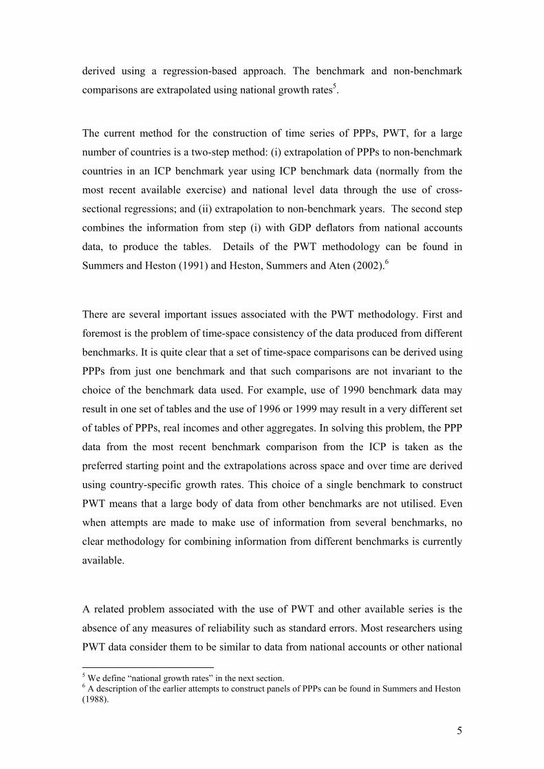
Case 2: Time Varying Intercept and Slopes (non-stochastic)
, with 0 when 1oit o ot ot
sit st
tβ β β β= + = ==β β
(27)
here,
0
02 0
1
1
[ ][ ... ][ ... ][ ( ... ) ]
o s
o T
s s sT
t N t N t Nt tj
θ θθ θ
′ ′ ′=′=
′ ′ ′=′ ′= ⊗
θ θθθ θ θX j e x x E
[ ... ... ] where, are K K zeros and is in the positiontht K K K K K t= ×E 0 I 0 0 I
Case 3: Time Varying Intercept and Slopes (stochastic)
, 1
, with 0 when 1oit o ot ot
sit st
st s t t
tβ β β β
−
= + = =
== +
β ββ β ε
(28)
In this case both the intercept and slopes are assumed to be time varying, and in
addition the evolution of the slopes follows a random walk. We incorporate stβ into
the state vector
* * * *1t t t t−= + +α α c η
where, * * *[ ] ; [ ] ; [ ]t t st t t t t t′ ′ ′ ′ ′ ′ ′ ′ ′= = =α α β c c 0 η η ε
* * *
*1
0 0
[ ( ... ) ]
[ ][ ]
t t t t t
t t t Nt
t N t N
θ
= + +
′=
′= ⊗
′ ′=
y Z α X δ ξ
Z Z x x
X j e jθ θ
18
Algorithm
There are two types of parameters to be estimated in the SS, namely,
hyperparameters, and coefficients associated with explanatory variables and the level
shifts. Hyperparameters are those associated with the covariance structure. In our
case these are: 2 2 2, , ,u η ξφ σ σ σ 18. These parameters must be estimated by numerical
maximization of the likelihood function (in a likelihood based estimation). The other
parameters, ,θ γ in our case, can be estimated by a generalised least squares procedure
in conjunction with the numerical maximization of the likelihood function (see
Harvey 1990 pp.130-133)19, or placed in the transition equation and estimated with
the state vector20.
Independently of which assumptions are made to identify itβ , the algorithm we use
can be described in 5 steps.
Step 1: Obtain an initial estimate of itβ , 0ˆitβ , by regressing tr on tX and construct an
initial prediction, 0ˆ itp , using equation (3).
Step 2: Run SS through KF (or KF/GLS) to obtain estimates of the hyperparameters
and ,θ γ .
Step 3: Use updated estimate of itβ , 00 0
ˆ ˆ ˆt t tβ β θ= − 0ˆ ˆ ˆ
sit sit sit= −β β θ , to obtain an
updated ˆ itp
Step 4: Repeat 2 and 3 until θ are sufficiently close to zero.
Step 5: Run KF and smoother one more time to obtain *ˆ itp and standard errors.
A prediction of PPPit is given by:
*
/ˆˆ it TpitPPP e= (29)
where,
18 and 2
εσ if Case 3 is used. 19 The SS in Cases 1 and 2 are set up for the use of the KF/GLS approach 20 The SS in Case 3 is set up to use this approach
19
*/ˆ it Tp is the corresponding element of * *
/ /ˆ ˆ= + t T t T tp α A γ , and
/t Tα is the smoothed estimate of the state-vector
The standard errors for the predicted PPP are computed as follows:
*
, ,/ ˆ ˆˆ2ˆ( ) ( 1)ii t ii tit Tpitse PPP e e eψ ψ= − (30)
where,
, /ˆ ˆis the diagonal element of the estimated covariance of the state vector, ii t t Tithψ α .
The next section presents an illustration of our proposed method.
5. An Empirical Application
In this section we present the results from the empirical implementation of our state-
space approach to construct a complete panel of PPPs for 23 OECD countries for the
period 1971 to 2000. We have accessed data for the OECD countries through the
OECD and World Bank sites. Several of the countries in the OECD were participants
in the ICP project since its first benchmark year. We include 23 countries in this
empirical illustration using the US as the reference country.
The sample used provides a unique opportunity to illustrate our method in that there
are a reasonable number of benchmark PPPs observations of the state variable for
most of these countries. In such a case it might be argued that a simple system
combining the benchmark data with the derived growth rates (equations (5) and (6))
should suffice to complete a panel of PPPs without requiring the predictions from the
national price level model. We construct such a panel by running the following
simplified state-space system (estimates and predictions from this model are labeled
as naïve model below):
Observation equations:
Non-benchmark years:
1= 0, = , = 0t t ty Z S ξ , E( ) =0t t t′ ≡ξ ξ H (31)
Benchmark years
20
11
0= , = , =t t t t
t t
⎡ ⎤⎡ ⎤⎢ ⎥⎢ ⎥
⎣ ⎦ ⎣ ⎦
Sy Z ξ ξ
p S%
( ) 2
0t t t
t t t
Eξσ
⎡ ⎤′ ≡ = ⎢ ⎥′⎣ ⎦
0ξ ξ H
0 S V S
Transition equations:
-1t t t t= + +p p c η
We then estimate the complete system under two alternatives. First, the state-space
model is estimated under the restriction that ICP benchmark data do not suffer from
any measurement error (we fix 2 1 10Eξσ = − , see equation (9)). However,
measurement error is allowed in the transition equations and spatial correlation in the
model of national price levels, and the results are labeled constrained model. Second,
the full state-space model is estimated allowing for measurement errors in the
benchmark and transition equations and spatial correlation in the model of national
price levels (results are labeled unconstrained model).
The data for the empirical example are for the period 1970 to 2000, annual, and we
discuss next the dependent, explanatory, and covariance related variables.
Dependent Variable
Benchmark PPP information, GDP Deflators, and exchange rates were collected from
the OECD website. Benchmark years were: 1980, 1985, 1990, 1993, 1996 and
199921. Table 1 lists the countries included in the analysis, the currency used and the
status of participation of each of the countries in various ICP Benchmark exercises of
the past.
21 We are indebted to Ms Francette Koechlin (OECD) for providing the ICP Benchmark data.
21
Explanatory Variables
The following variables were included as explanatory variables in the national price
level model:
Euro Dummy: Takes the value of 1 from 1993 onwards for the countries that joined
the euro currency by 2000.
FDI%: Foreign direct investment, net inflows (% of GDP)
LE: Life Expectancy in years
SERV%: Services, value added (% of GDP)
OPEN%: Trade (% of GDP)
CPIit/CPIUS,t, for i= 1, …, N
Labour Productivity = (Population × per capita GDP)/ Labour Force
The choice of conditioning variables is based on national price level theory and data
availability. The data were obtained from the OECD website and from various issues
of the World Development Indicators published by the World Bank on a regular basis
The statistical model and the variables included in the regression equation are adapted
from those used in the literature to suit the nature and scope of the current study. In
particular, since the model is only illustrative and is applied only to OECD countries,
a variable like education has not been included. The effect of productivity differentials
on national price levels is captured through the inclusion of a labour productivity
measure. The model is a first approximation and further work and refinements are
planned for the next stage of this project.
Identifying Assumptions
The illustration has been obtained using the identifying assumptions presented in Case
1 (See equation (26)). Additionally, for the purpose of this illustration γ (see equation
(12)) is assumed to be zero.
Covariance related Variables
a) Measuring spatial correlation
22
A contiguity matrix was constructed using volumes of bilateral trade in 1990.
This is the matrix W (see equation (8)).
b) Capturing accuracy of benchmark data collection and National Accounts’
computation of the national price level.
We assume that the measurement error in the collection of PPP benchmark data and in
the growth rate on the GDP deflator are uncorrelated. However, in both cases they are
assumed to be distributed with a zero mean and heteroskedastic with a diagonal
covariance which is inversely related to the real per capita (measured in constant US$
of 1995) of the country.
Distribution of the Initial State Vector
We note that under the assumption =γ 0 , the state vector simplifies to (see equation
(22):
= t tα p
For this specification we can derive a non-diffuse covariance for the initial state
vector, = o oα p by making use of equation (3). Suppose at t = 0 we have socio-
economic data, Xo. Then we can define,
ln( )o o o o= + +p X β ER u (32)
where,
[ ]oo so ′=β β β
(1)
(2)o
oo
⎡ ⎤= ⎢ ⎥⎣ ⎦
pp
p
(1)
(2)o
oo
⎡ ⎤= ⎢ ⎥⎣ ⎦
XX
X
(1)oX and (1)
op are the corresponding partition containing the observations from
participating countries.
Then a prediction of op and its associated covariance are given by
ˆˆ ln( )o o o= +p X β ER (33)
23
2 (1) (1) 1ˆcov( ) ( )o o o o o oσ −′ ′= =p Ψ X X X X (34)
We use the expression in (34) to obtain an estimate of the covariance of the initial
state vector for the constrained and unconstrained models. For the naïve model we
use a diffuse prior.
5.1 Model Estimates
Table 2 presents the parameter estimates with standard errors. Data for 1970 were
used to create growth rates where needed, data for 1971-2000 were used for
estimation. The years 1971 and 1972 are used as burning off periods22, and therefore
not reported in the predictions.
The computed likelihood ratio test for the null hypothesis that the constrained model
is correct (Table 2) is statistically significant at the 1% level and therefore the
restriction that benchmark data do not suffer from measurement error is rejected by
the data (we still present both sets of predictions in the next section for comparison).
The time varying intercept shows a slight downward trend over time. All slope
parameters are statistically significant and with expected signs with the exception of
FDI.
5.2 Predictions of PPP
The methodology proposed generates a complete matrix of PPPs for all the 23
countries and for all the years. In order to facilitate presentation and discussion, we
have chosen three countries, Australia, Spain and Turkey. These countries have been
chosen for illustrating the PPP predictions obtained, and for the purpose of comparing
to alternative predictions from other approaches. The reason for this choice is that
Australia floated its exchange rate in 1984, providing an excellent opportunity to test
our approach during a volatile exchange rate period. Spain is chosen to represent the
countries that joined the euro-zone and have participated in all ICP benchmark
exercises to date. Finally, Turkey is chosen as it is a country exhibiting hyperinflation 22 This is particularly important when the covariance of the initial state vector is diffuse.
24
during the sample period providing a challenge to any modeling approach23.
Therefore, selection of Turkey is designed to assess the performance of the method
when the country under consideration exhibits extreme price movements.
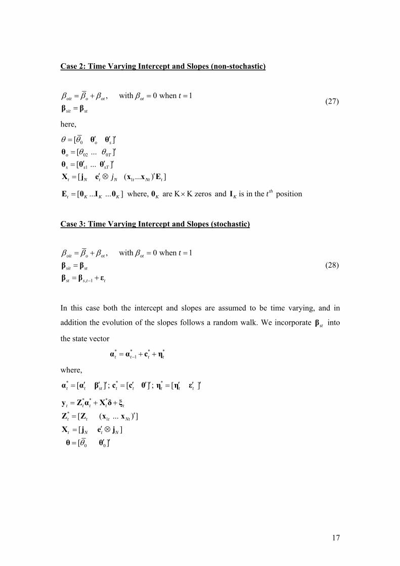
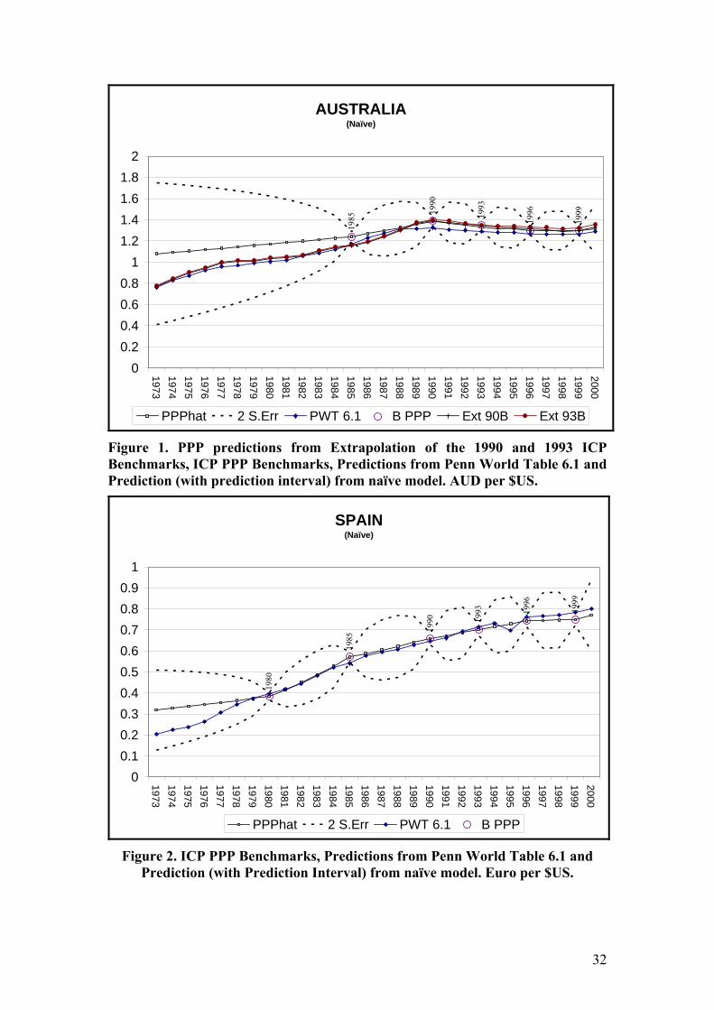
The results are presented in graphical (for Australia and Spain) and table format (for
Turkey). Figures 1 and 2 present the predictions from the naïve model for Australia
and Spain, respectively. Figures 3 and 4 present the predictions from the constrained
model, and Figures 5 and 6 those from the unconstrained model for Australia and
Spain, respectively. Table 3 presents the results for Turkey.
All figures for Australia include PPP predictions computed under three alternative
approaches. The first type is the time series of PPPs that can be computed by
extrapolating a given benchmark ICP value using the implied growth rate (see
equation (4)). One such series can be produced for each country and benchmark year.
We present only two of those for illustration, labeled EXT 93B and EXT 90B. They
are the extrapolations obtained using the 1990 and 1993 ICP benchmark values,
respectively. The second type of predictions is that produced by the Penn World
Tables (PWT 6.1). These are presented so that our results can be benchmarked
against what is currently commonly used. They are plotted for Australia and Spain
and included in Table 3 for Turkey to offer a comparison. Finally, the predictions
computed using our approach are presented for all three countries (including a
±2×Standard Error interval for Australia and Spain and the standard errors for
Turkey).
From the results we note that prediction intervals increase in size when the time
period under consideration is away from a benchmark year, and reduce significantly at
the benchmarks even for models that are unrestricted. The naïve model’s prediction
interval is useful in highlighting this issue. For the early years of the sample, when no
observations on the state variable are available through ICP benchmarking, prediction
intervals are extremely wide. The inclusion of predictions from the national price
level model becomes crucial in reducing uncertainty. Comparing Figures 1 to 3 and 5,
or Figures 2 to 4 and 6 this can be observed. Further, for the case of Turkey, see Table
23 A complete tableau is available from the authors.
25
3, it is clear that the absence of ICP benchmarks and predictions from the national
price level model for the early period results in implausible PPPs predictions from the
naïve model. The estimates are much larger than the exchange rate when they would
be expected to be smaller so the resulting ratio PPP/ER is less than one. This is the
case for the estimates produced by the two full models. That is, when comparing
predictions and standard errors of the naïve model to those of the full system for all
three countries it is evident that the full models are superior to the naïve model. As
stated in the introduction, most countries in the world have participated in the current
round of the ICP benchmarking for the first time24. Thus, the inclusion of the national
price level model in the state-space formulation is crucial to both the prediction of the
mean value of PPPs as well as its variance.
Concentrating now on the predictions from the full state-space, we note that the
prediction interval for benchmark years is much wider in the unconstrained than the
constrained case (this can be easily observed from Table 3), while the PPP point
prediction for the benchmark value differs minimally from the actual benchmark PPPs
for Australia and Spain. These are predictions that quantify and weigh the
measurement error from all sources of information.
Figures 1, 3, 5, and 7 present results for Australia. Figure 7 superimposes the
movements of the exchange rate over the sample period (ER) on the PPP series
produced by the PWT and our unconstrained model. This figure is included to
demonstrate that PPP predictions are a smoother series than the exchange rate as
expected. After the floating of the AUD in 1984, the ER experienced some highly
volatile periods. This structural change in the ER is reflected in the movement of the
PPPs. The volatility of the exchange rates combined with the absence of benchmark
information before 1985 result in a wider prediction intervals (Figures 1, 3 and 5),
although much narrower than those of the naïve model. The extrapolated series (from
1990 and 1993 benchmarks) plotted in Figures 1, 3 and 5 demonstrate how difficult it
is to produce point predictions in this situation, given the inconsistency across
observation sources and time. Thus, the use of an interval estimate, similar to that
24 Preliminary estimates from the current ICP round, carried out in 2005, have still not been released at the time of submission of this manuscript.
26
provided by our method, should provide users of the panel with a way of assessing
“best” and “worse” case scenario in further applied work.
The predictions for Spain are very representative of most of the “core” OECD group
of countries that participated in the ICP from the beginning and are mostly European
Union members. Predictions from our model are very close to those produced by the
Penn World Table and the later is inside our computed prediction interval for most
periods.
Turkey exhibited hyperinflation during most of the sample period. Table 3 shows the
explosive increase in the market exchange rate which is reflected in the Benchmark
estimates of the ICP. We note the accuracy of our predictions in following this trend,
and as mentioned before, the much wider prediction interval estimates for benchmark
years obtained from the naïve model.
6. Conclusions
The main objective of the paper is to propose an econometric model using the state-
space approach which can be employed in the estimation of a panel of purchasing
power parities necessary for constructing a consistent set of internationally
comparable real income aggregates. The methodology described here successfully
combines data drawn from a number of national and international sources in
estimating PPPs. It offers several improvements over the existing PWT approach,
which is the only source of such data at the present time. These improvements include
a method that: (i) can make use of all the PPP data from the ICP for all the
benchmark years since 1970; (ii) can provide optimal predictors for PPPs for ICP-
non-participating countries and for non-benchmark years; (iii) produces PPPs that are
consistent with observed movements in prices in different countries; and (iv) provides
standard errors associated to the PPPs and, therefore, for the estimates of real per
capita incomes. To achieve these objectives the paper proposes the use of an
econometric model with errors that are spatially correlated cross-sectionally and
accounts for measurement error in the available sources of data. The econometric
model is re-formulated in a state-space form and estimated using Kalman filtering
techniques. The new methodology is applied to an illustrative data set of 23 OECD
27
countries for the period 1970 to 2000. The results from the illustrative application
demonstrate the feasibility of using the model for consistent space-time extrapolation.
The main conclusion from the paper is that it is feasible to develop a more
comprehensive econometric approach to the construction of a panel of PPPs than the
current practice in constructing extrapolations of PPPs. It is also important to note that
the approach proposed here makes optimal use of relevant information from diverse
sources and the methodology provides standard errors and, therefore, measures of
reliability of predicted values of PPPs.
28
References Ahmad, S. (1996), "Regression Estimates of per Capita GDP Based on Purchasing
Power Parities", in International Comparisons of Prices, Output and Productivity, in Salazar-Carrillo and D.S. Prasada Rao (eds.), Contributions to Economic Analysis Series, North Holland.
Barro, R J, and X Sala-i-Martin (2004) Economic Growth (Second ed.). Cambridge MA: MIT Press.
Bergstrand, J.H, (1991), “Structural determinants of real exchange rates and national price levels”, American Economic Review, 81, 325-334.
Bergstrand, J.H. (1996), “ Productivity, Factor Endowments, Military Expenditures, and National Price Levels” in International Comparisons of Prices, Ouput and Productivity, D.S. Prasada Rao and J. Salazar-Carrillo (eds.), Elsevier Science Publishers B.V. North Holland.
Castles, I. and D. Hendersen (2003), IPPC Issues: A Swag of Documents, URL: http://www.lavoisier.com.au/papers/articles/IPPCissues.html (as on 14 December, 2007).
Clague, C.K.(1988) “Explanations of National Price Levels,” in World Comparison of Incomes, Prices and Product, J. Salazar-Carrillo and D.S. Prasada Rao (eds.), Elsevier Science Publishers B.V, North Holland.
Durbin, J and S. J. Koopman (2001) Time Series Analysis by State Space Methods. Oxford University Press.
(2002) “A Simple and Efficient Simulation Smoother for State Space Time Series Analysis”. Biometrika 89, 603-616.
Durlauf, S N, et al. (2005) 'Growth Econometrics. In Aghion, P and S N Durlauf (Eds.), Handbook of Economic Growth (Vol. 1, pp. 555-677). Amsterdam: Elselvier.
Harvey, A. C. (1990), Forecasting, Structural Time Series Models and the Kalman Filter, Cambridge Univ. Press. Cambridge.
Harvey, A.C., Thomas M. Trimbur, and Herman K. van Dijk (2005) “Trends and Cycles in Economic Time Series: A Bayesian Approach” manuscript.
Heston, A., R. Summers and B. Aten, Penn World Table Version 6.1, Center for International Comparisons at the University of Pennsylvania (CICUP), October 2002.
Koop, G. and H.K. van Dijk (2000) “Testing For Integration Using Evolving Trend and Seasonal Models: A Bayesian Approach” Journal of Econometrics 97, 261-91.
Kravis, Irving B., and R E. Lipsey (1983) “Toward an Explanation of National Price Levels,” Princeton Studies in International Finance, No 52 Princeton, N.J.: Princeton University, International Finance Section.
Kravis, Irving B., and R E. Lipsey (1986), “The Assessment of National Price Levels,” Paper presented at Eastern Economic Association Meetings, Philadelphia, April.
Kravis I.G., Summers, R. and A.W. Heston (1982), World Product and Income, Johns Hopkins University Press, Baltimore.
McKibbin, W.J., and A. Stegman, 2005, “Convergence and Per Capita Carbon Emissions”, Working Paper No. 04.05, Lowey Institute for International Policy, Sydney, Australia.
Maddison, A. (1995), Monitoring the World Economy, 1820-1992, OECD, Paris.
29
Maddison, A. (2007), Contours of the World Economy 1—2030 AD: Essays in Macro-
Economic History, Oxford, U.K. Milanovic, B. (2002), “True World Income Distribution, 1988 and 1993: First
Calculation Based on Household Surveys Alone,” The Economic Journal, 112, 51-92.
Sala-i-Martin, X. X. (2002). 15 Years of New Growth Economics: What have we learnt? Unpublished manuscript.
Summers, R. and A. Heston (1988), "Comparing International Comparisons", in World Comparisons of Incomes, Prices and Product, (eds.) Salazar-Carrillo and D.S. Prasada Rao, Contributions to Economic Analysis Series, North-Holland. Summers, R. and A. Heston (1991), “The Penn World Tables (Mark 5): An expanded set of international comparisons, 1950-88”, Quarterly Journal of Economics, 2, 1-45.
UNDP (2006), Human Development Report 2006, United Nations Development Program, New York, USA.
World Bank (2006), World Development Indicator 2006s, World Bank, 2006 and other years, Washington DC.
30
Table 1. Countries, Currency and their status of the ICP Participation
COUNTRY CURRENCY ICP PARTICIPATION
Australia AUS Australian dollar 1985, 1990, 1993, 1996, 1999
Austria AUT Euros (1999 ATS euro)a 1980, 1985, 1990, 1993, 1996, 1999
Canada CAN Canadian dollar 1980, 1985, 1990, 1993, 1996, 1999
United States US US dollars Reference country a Pre-Euro domestic currencies were converted using the 1999 Irrevocable Conversion Rate (Source: http://www.ecb.int/press/pr/date/1998/html/pr981231_2.en.html) b The irrevocable conversion rate of the drachma vis à vis the euro was set at GRD 340.750. Source: http://www.bankofgreece.gr/en/euro/
Figure 1. PPP predictions from Extrapolation of the 1990 and 1993 ICP Benchmarks, ICP PPP Benchmarks, Predictions from Penn World Table 6.1 and Prediction (with prediction interval) from naïve model. AUD per $US.
Figure 3. PPP predictions from Extrapolation of the 1990 and 1993 ICP Benchmarks, ICP PPP Benchmarks, Predictions from Penn World Table 6.1 and Prediction (with Prediction Interval) from constrained model. AUD per $US.
Figure 5. PPP predictions from Extrapolation of the 1990 and 1993 ICP Benchmarks, ICP PPP Benchmarks, Predictions from Penn World Table 6.1 and Prediction (with Prediction Interval) from unconstrained model. AUD per $US.