Centrifugal Compressor Modelling with a Particle Filter ... · 1.2 ABB turbocharger structure ... a...

POLITECNICO DI MILANO

Master Degree in Automation and Control Engineering

School of Industrial and Information Engineering

Centrifugal Compressor Modelling with a Particle

Filter Application for Optimal Estimation in

Turbochargers

Supervisor :

Prof. Sergio Bittanti

Co-supervisors:

Ing. Antonio De Marco

Ing. Diego Pareschi

Author :

Mirko Casnedi

r.n. 804751

Academic year 2015-2016

Sommario

Negli ultimi decenni i turbocharger hanno trovato ampia diffusione e inno-

vazione tecnologica in diversi tipi di applicazioni e settori, tra i quali ricopre

un ruolo di primaria importanza quello della sovralimentazione di motori

Diesel. E importante per il corretto funzionamento di un turbocharger che

il compressore centrifugo e la turbina, le due turbomacchine che lo costituis-

cono, lavorino in condizioni di alta efficienza, cioe lontano da punti di lavoro

con perdite elevate o addirittura instabili. Per questa ragione risulta chiara

l’utilita di disporre di un sistema di monitoraggio al fine di stabilire in ogni

istante di tempo il punto di lavoro di entrambe le turbomacchine. In certe

situazioni alcune misure utili per il monitoraggio possono essere non disponi-

bili per varie ragioni, come punti difficilmente raggiungibili all’interno della

macchina o soggetti a forti sollecitazioni meccaniche e termiche, motivo da

cui nasce la necessita di impostare una procedura di stima atta a compensare

questa mancanza. Il presente lavoro di tesi, sviluppato in collaborazione con

ABB S.p.a (Sesto San Giovanni), si compone di due parti principali. Nella

prima parte viene presentata la teoria e la filosofia per la modellistica fisica di

un compressore centrifugo, nella quale la macchina e pensata come costituita

da diversi stadi in cui possono essere applicate le leggi della termodinamica

e della fluidomeccanica al fine di ricavare l’andamento delle variabili che de-

scrivono il flusso del fluido al suo interno. Il modello e quindi validato ed

utilizzato per l’analisi di alcuni tipi di perdite caratteristiche dei compressori.

Successivamente viene ricavato un modello alternativo a partire dalla mappa

caratteristica del compressore, utile ogniqualvolta i parametri geometrici del

compressore fossero sconosciuti. Nella seconda parte viene invece presentata

la teoria del Particle Filtering, tecnica di filtraggio appartenente alla classe

dei filtri bayesiani non lineari. Tale metodo di filtraggio e quindi applicato,

insieme al modello del compressore, per ricavare delle stime ottime della

portata volumetrica, pressioni e temperature non misurate nel turbocharger

del caso in esame. Infine viene presentato un modello semplificato per la

turbina assiale ed una possibile procedura di stima con il Particle Filter.

Abstract

In the last decades turbochargers have seen a huge spreading and techno-

logical innovation in several fields and applications, most of all in Diesel

combustion engine supercharging. It is important for the correct operation

of turbochargers that the centrifugal compressor and turbine, the two tur-

bomachines by which it is constituted, work at high efficiency condition, i.e.

far enough from regions with high losses or even unstable. For this reasons

is clear the necessity for turbochargers monitoring, in order to establish at

each time the working point of both the turbomachines. Sometimes some

measures necessary for a correct monitoring may be not available for sev-

eral reasons, such as points difficult to reach or subject to high mechanical

and thermal stresses, from which arises the need to derive an estimation

procedure to counteract this lack. This thesis, developed in collaboration

with ABB S.p.a (Sesto San Giovanni), consists of two main parts. The

first part presents the theory and the philosophy for centrifugal compressors

modelling, in which the turbomachine is thought as constituted by a series

of ducts where the fundamental laws of termodynamics and fluid mechanics

can be applied to infer the flow conditions. The model is applied, validated

and utilized to analyse some kind of losses occurring in the compressor. Next

an alternative model, useful when geometrical data are not available, is built

interpolating some points extracted from an experimental map provided by

ABB. In the second part, the theory of non-linear Bayesian Particle Filter

is presented. Next a statistical analysis of the available experimental data

is made. The particle filter is then employed together with the compressor

model to optimally estimate non-measured flow rates, pressures and temper-

atures in the turbocharger. Lastly a simplified model for the axial turbine

is introduced and a possible filtering procedure is outlined.

a Mamma e Papa

Contents

1 Introduction 1

1.1 Operation principles of turbochargers . . . . . . . . . . . . . 1

1.2 Turbocharger structure . . . . . . . . . . . . . . . . . . . . . . 3

1.3 Types of turbocharging . . . . . . . . . . . . . . . . . . . . . 4

1.3.1 Constant pressure turbocharging . . . . . . . . . . . . 4

1.3.2 Pulse system turbocharging . . . . . . . . . . . . . . . 4

1.4 Problem statement and motivation . . . . . . . . . . . . . . . 5

1.4.1 Case study: Marseglia generation plant . . . . . . . . 5

1.4.2 Monitoring system . . . . . . . . . . . . . . . . . . . . 6

1.4.3 Sensoring layout . . . . . . . . . . . . . . . . . . . . . 7

1.5 Structure of the thesis . . . . . . . . . . . . . . . . . . . . . . 8

2 Centrifugal Compressor Modelling 11

2.1 Motivation for physical compressor modelling . . . . . . . . . 11

2.1.1 1D Modelling . . . . . . . . . . . . . . . . . . . . . . . 12

2.2 Compressor structure . . . . . . . . . . . . . . . . . . . . . . 12

2.3 Preliminary tools and conventions . . . . . . . . . . . . . . . 14

2.3.1 Coordinate system . . . . . . . . . . . . . . . . . . . . 14

2.3.2 Absolute and relative velocities . . . . . . . . . . . . . 14

2.3.3 Sign convention . . . . . . . . . . . . . . . . . . . . . . 16

2.4 Isentropic modelling . . . . . . . . . . . . . . . . . . . . . . . 16

2.4.1 The stagnation state . . . . . . . . . . . . . . . . . . . 16

2.4.2 The relative stagnation state and Rothalpy . . . . . . 18

2.4.3 Adimensional Mass Flow Rate Equation . . . . . . . . 18

2.4.4 Use AME to calculate fluid flow process . . . . . . . . 19

2.4.5 Slip factor . . . . . . . . . . . . . . . . . . . . . . . . . 20

2.4.6 Non-guided swirling flow . . . . . . . . . . . . . . . . . 21

2.5 Compressor losses . . . . . . . . . . . . . . . . . . . . . . . . 22

2.5.1 Compressor efficiency . . . . . . . . . . . . . . . . . . 22

2.5.2 Physics of loss mechanisms . . . . . . . . . . . . . . . 24

iii

2.5.3 Loss coefficients . . . . . . . . . . . . . . . . . . . . . . 26

2.6 Model structure . . . . . . . . . . . . . . . . . . . . . . . . . . 28

2.6.1 Isentropic flow . . . . . . . . . . . . . . . . . . . . . . 30

2.6.2 Loss coefficients calculations . . . . . . . . . . . . . . . 32

2.6.3 Correction step for actual flow . . . . . . . . . . . . . 32

3 Model Validation and Losses Analysis 35

3.1 Compressor map . . . . . . . . . . . . . . . . . . . . . . . . . 35

3.2 Validation of the model . . . . . . . . . . . . . . . . . . . . . 37

3.3 Geometrical parameters identification . . . . . . . . . . . . . 39

3.4 Isentropic and actual maps . . . . . . . . . . . . . . . . . . . 40

3.5 Loss analysis . . . . . . . . . . . . . . . . . . . . . . . . . . . 41

3.5.1 Impeller skin friction loss . . . . . . . . . . . . . . . . 41

3.5.2 Impeller incidence loss . . . . . . . . . . . . . . . . . . 43

3.5.3 Blade loading loss . . . . . . . . . . . . . . . . . . . . 45

3.6 Conclusion on physical compressor modelling . . . . . . . . . 45

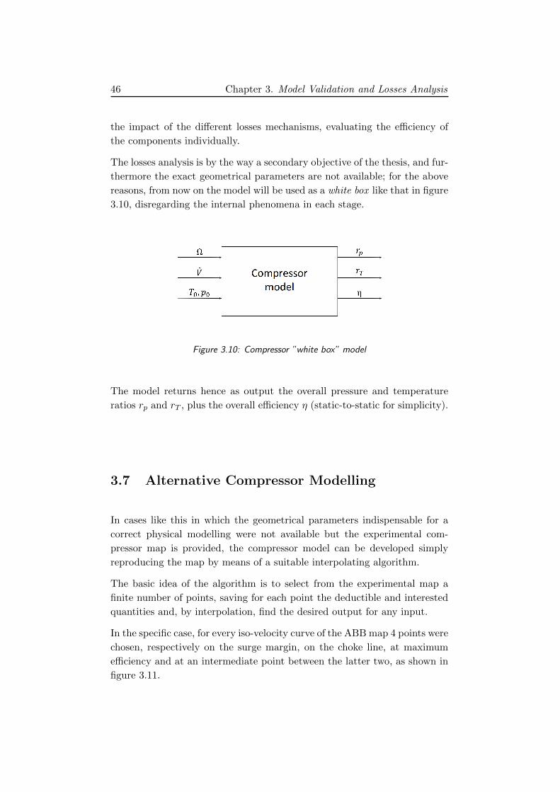
3.7 Alternative Compressor Modelling . . . . . . . . . . . . . . . 46

3.7.1 Results . . . . . . . . . . . . . . . . . . . . . . . . . . 48

4 Theory of Particle Filtering 49

4.1 Models and notation . . . . . . . . . . . . . . . . . . . . . . . 49

4.2 Optimal estimation . . . . . . . . . . . . . . . . . . . . . . . . 50

4.3 Particle Filter Theory . . . . . . . . . . . . . . . . . . . . . . 51

4.3.1 A priori distribution approximation . . . . . . . . . . 52

4.3.2 A posteriori distribution approximation . . . . . . . . 53

4.3.3 Conditional expectation . . . . . . . . . . . . . . . . . 54

4.4 Particle Filter Algorithm summary . . . . . . . . . . . . . . . 55

5 Particle Filter Application 57

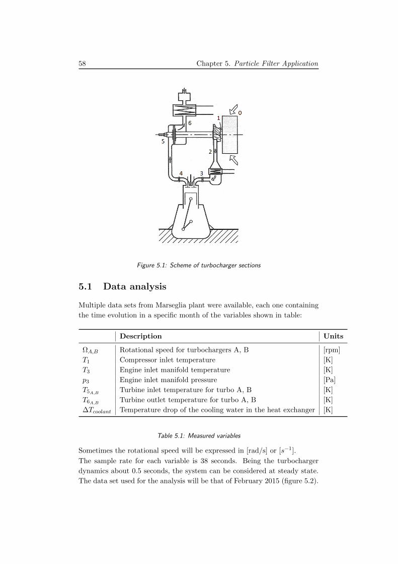
5.1 Data analysis . . . . . . . . . . . . . . . . . . . . . . . . . . . 58

5.1.1 Filtering and normalization . . . . . . . . . . . . . . . 60

5.1.2 Principal Component Analysis . . . . . . . . . . . . . 61

5.2 Compressor Filtering . . . . . . . . . . . . . . . . . . . . . . . 62

5.2.1 Model and prior pdfs . . . . . . . . . . . . . . . . . . . 62

5.2.2 Normalization . . . . . . . . . . . . . . . . . . . . . . . 66

5.2.3 Filtering for t > 0 . . . . . . . . . . . . . . . . . . . . 66

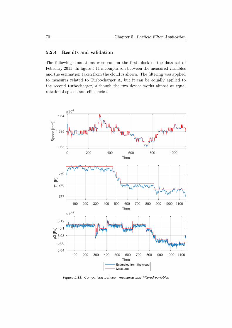
5.2.4 Results and validation . . . . . . . . . . . . . . . . . . 70

5.3 Turbine Filtering overview . . . . . . . . . . . . . . . . . . . . 75

6 Conclusions 79

Appendices 81

A Fluid mechanics and thermodynamics equations 83

A.1 Thermodynamic properties of perfect gas . . . . . . . . . . . 83

A.2 Continuity equation . . . . . . . . . . . . . . . . . . . . . . . 83

A.3 First law of thermodynamics . . . . . . . . . . . . . . . . . . 84

A.4 Second law of thermodynamics . . . . . . . . . . . . . . . . . 85

A.5 Moment of momentum - Euler’s turbomachinery equation . . 85

A.6 Compressible flow relations for perfect gases . . . . . . . . . . 86

B Probability and Statistics 87

B.1 Probability density function . . . . . . . . . . . . . . . . . . . 87

B.2 Conditional density (of x given y) . . . . . . . . . . . . . . . . 88

B.3 Bayes update recursion . . . . . . . . . . . . . . . . . . . . . . 88

C Centrifugal compressor data set for validation 91

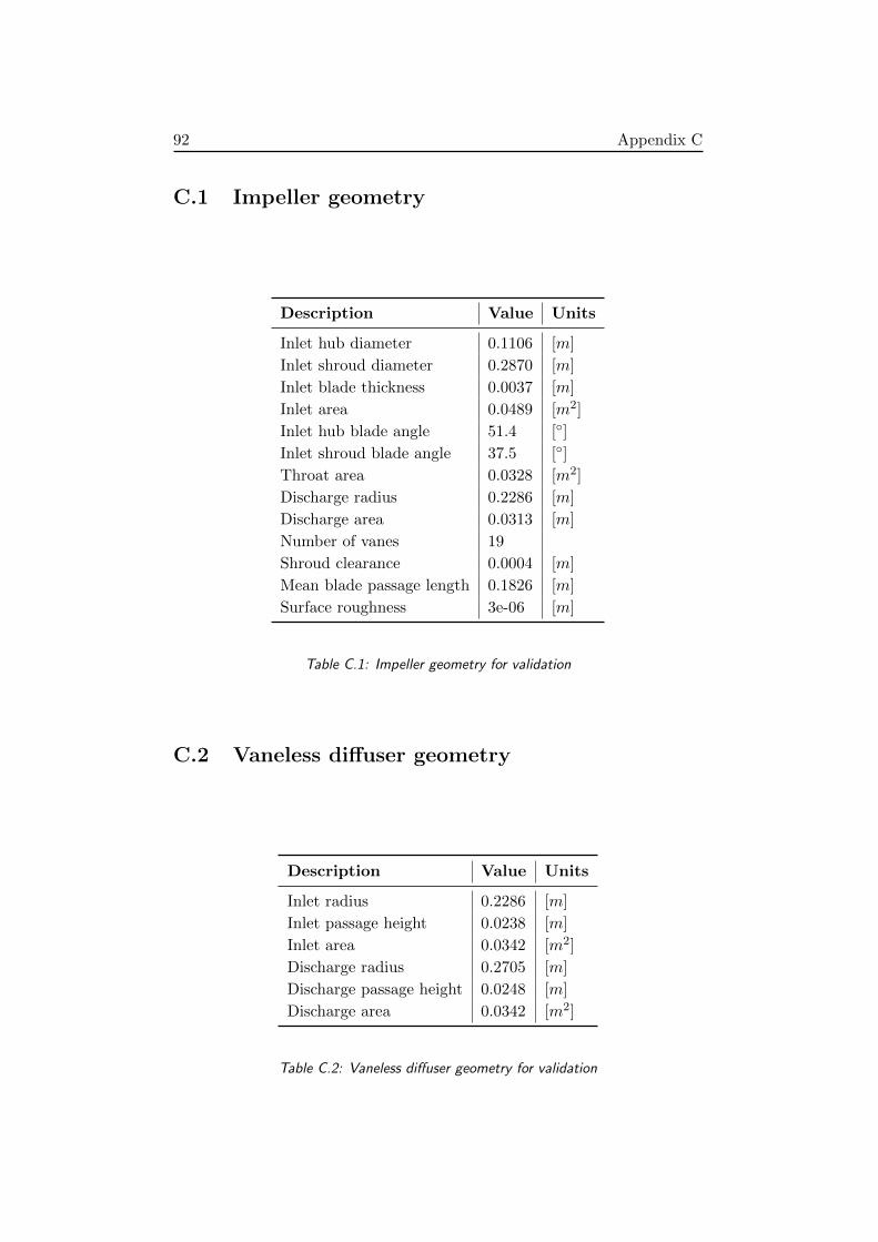
C.1 Impeller geometry . . . . . . . . . . . . . . . . . . . . . . . . 92

C.2 Vaneless diffuser geometry . . . . . . . . . . . . . . . . . . . . 92

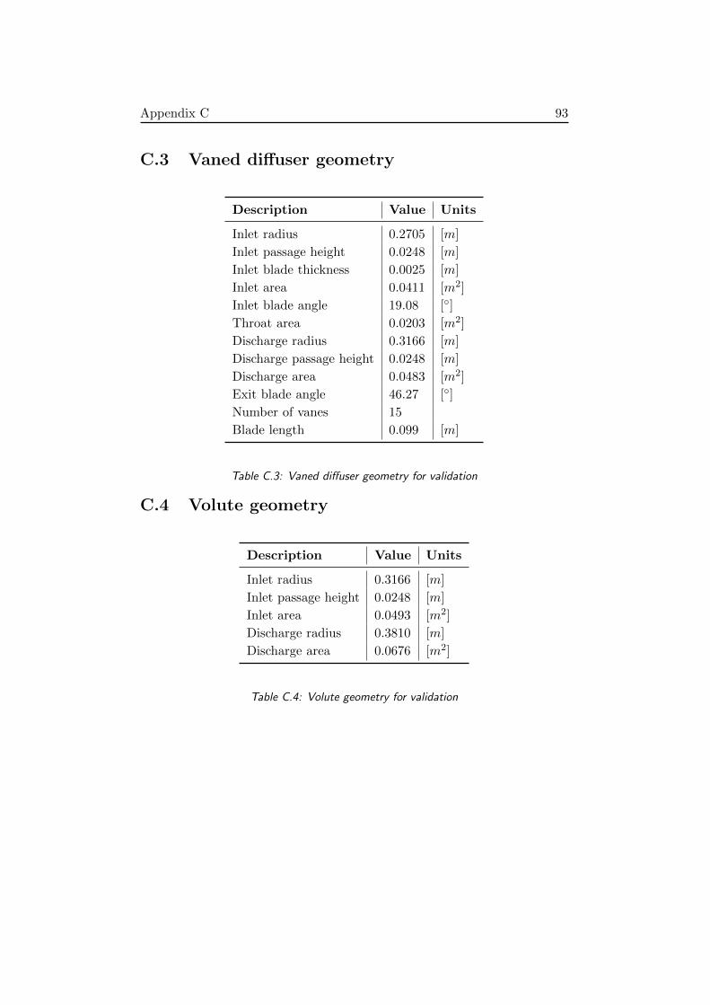
C.3 Vaned diffuser geometry . . . . . . . . . . . . . . . . . . . . . 93

C.4 Volute geometry . . . . . . . . . . . . . . . . . . . . . . . . . 93

List of Figures

1.1 Comparison between p-V diagrams of naturally aspirated and

supercharged engine . . . . . . . . . . . . . . . . . . . . . . . 2

1.2 ABB turbocharger structure . . . . . . . . . . . . . . . . . . . 3

1.3 Engine room overview . . . . . . . . . . . . . . . . . . . . . . 5

1.4 Turbocharged engine control loop . . . . . . . . . . . . . . . 6

1.5 Sensoring layout . . . . . . . . . . . . . . . . . . . . . . . . . 8

2.1 ABB TPL-77 impeller . . . . . . . . . . . . . . . . . . . . . . 13

2.2 Cross-sectional view of centrifugal compressor . . . . . . . . . 13

2.3 Cross-sectional view with inlet and outlet velocity triangles [1] 15

2.4 Coordinate system and flow velocities within a turbomachine.

a) Meridional or side view b) Axial view c) Vie looking down

onto a stream surface [1] . . . . . . . . . . . . . . . . . . . . . 16

2.5 AME diagram . . . . . . . . . . . . . . . . . . . . . . . . . . . 19

2.6 Velocity triangles with and without slip . . . . . . . . . . . . 21

2.7 Mollier diagram for compression process in the impeller . . . 23

2.8 Jet and wake velocity profiles at impeller discharge . . . . . . 26

2.9 Model structure . . . . . . . . . . . . . . . . . . . . . . . . . . 28

2.10 Isentropic model diagram . . . . . . . . . . . . . . . . . . . . 29

2.11 Scheme for actual flow computation . . . . . . . . . . . . . . 33

3.1 ABB Compressor characteristic map . . . . . . . . . . . . . . 36

3.2 Isentropic model and experimental data comparison . . . . . 37

3.3 Model with losses and experimental data comparison . . . . . 38

3.4 Compressor isentropic map . . . . . . . . . . . . . . . . . . . 40

3.5 Comparison between model output and experimental maps . 41

3.6 Entropy variation due to skin friction loss for different rota-

tional speeds . . . . . . . . . . . . . . . . . . . . . . . . . . . 43

3.7 Entropy variation due to incidence loss for different rotational

speeds . . . . . . . . . . . . . . . . . . . . . . . . . . . . . . . 44

vii

3.8 Comparison between relative inlet flow angle and inlet blade

angle for different rotational speeds . . . . . . . . . . . . . . . 44

3.9 Entropy variations in blade loading loss . . . . . . . . . . . . 45

3.10 Compressor ”white box” model . . . . . . . . . . . . . . . . . 46

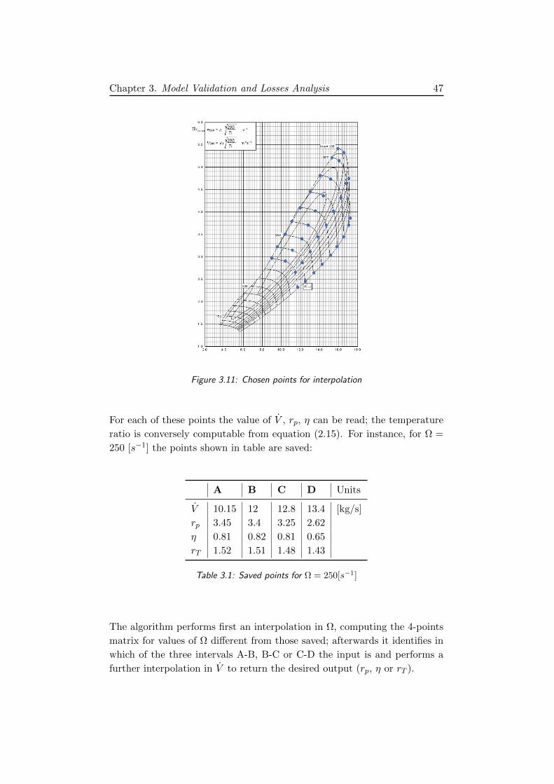
3.11 Chosen points for interpolation . . . . . . . . . . . . . . . . . 47

3.12 Efficiency, pressure ratio and temperature ratio functions . . 48

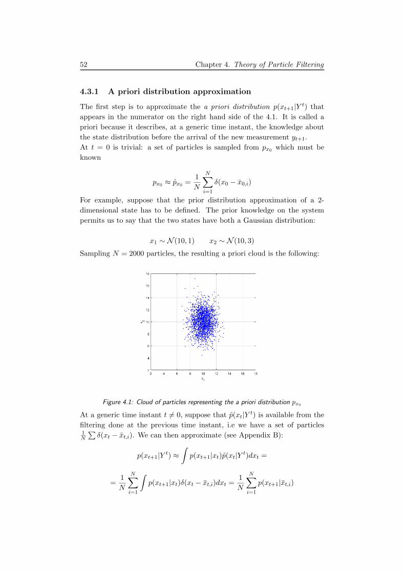
4.1 Cloud of particles representing the a priori distribution px0 . 52

5.1 Scheme of turbocharger sections . . . . . . . . . . . . . . . . 58

5.2 Set of measures available . . . . . . . . . . . . . . . . . . . . . 59

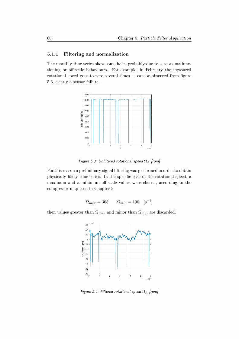
5.3 Unfiltered rotational speed ΩA [rpm] . . . . . . . . . . . . . . 60

5.4 Filtered rotational speed ΩA [rpm] . . . . . . . . . . . . . . . 60

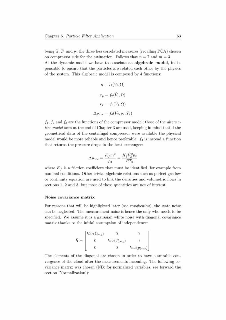
5.5 Prior density of input variables . . . . . . . . . . . . . . . . . 64

5.6 Prior density of input variables after the elimination of un-

feasible particles . . . . . . . . . . . . . . . . . . . . . . . . . 65

5.8 Scheme of normalization/denormalization procedure . . . . . 66

5.7 Projections of 7-dimensional cloud on some relevant planes . 67

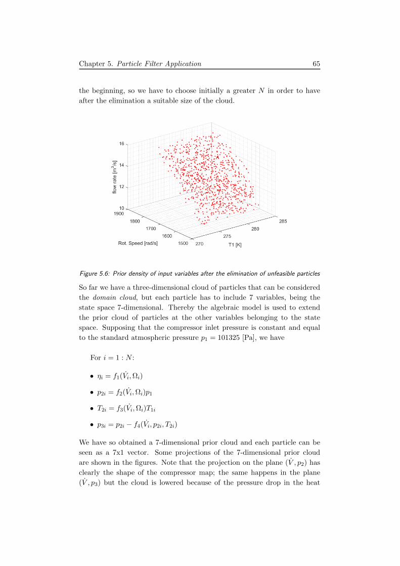
5.9 Sample impoverishmentin in 4 iterations . . . . . . . . . . . . 68

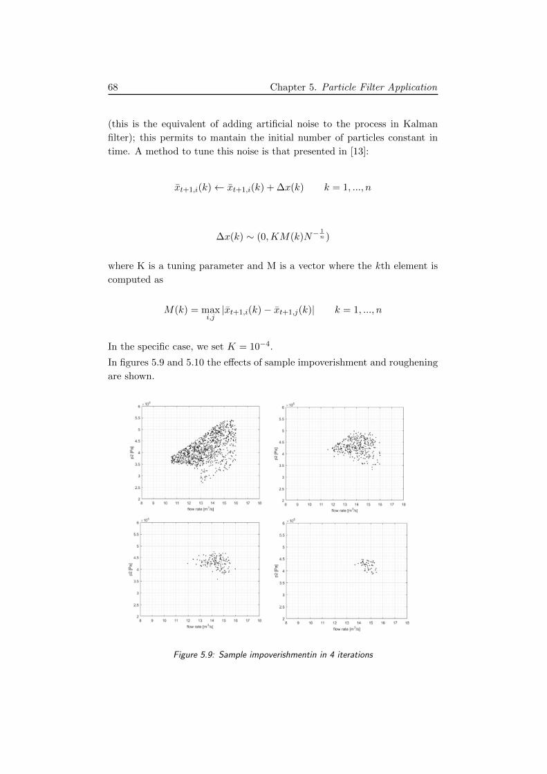
5.10 Effect of roughening . . . . . . . . . . . . . . . . . . . . . . . 69

5.11 Comparison between measured and filtered variables . . . . . 70

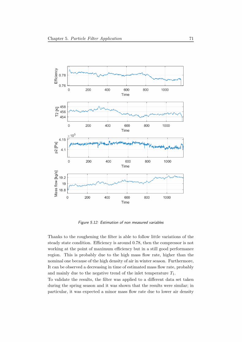
5.12 Estimation of non measured variables . . . . . . . . . . . . . 71

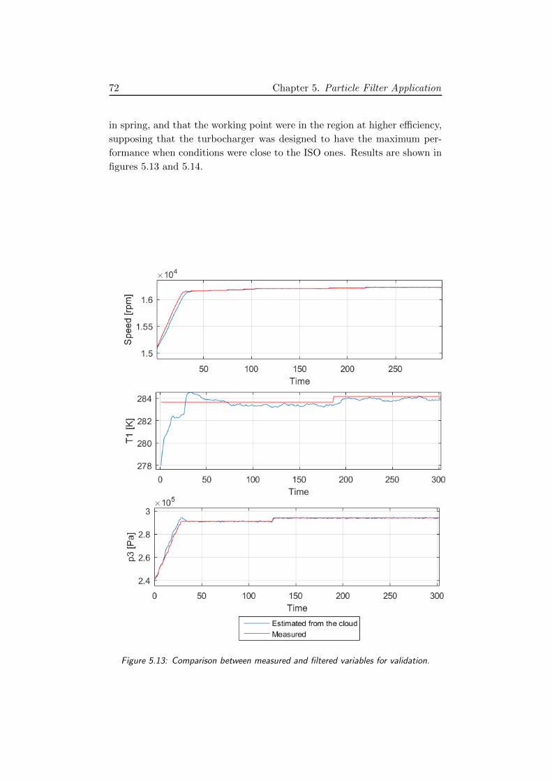
5.13 Comparison between measured and filtered variables for val-

idation. . . . . . . . . . . . . . . . . . . . . . . . . . . . . . . 72

5.14 Estimation of non measured variables for validation. . . . . . 73

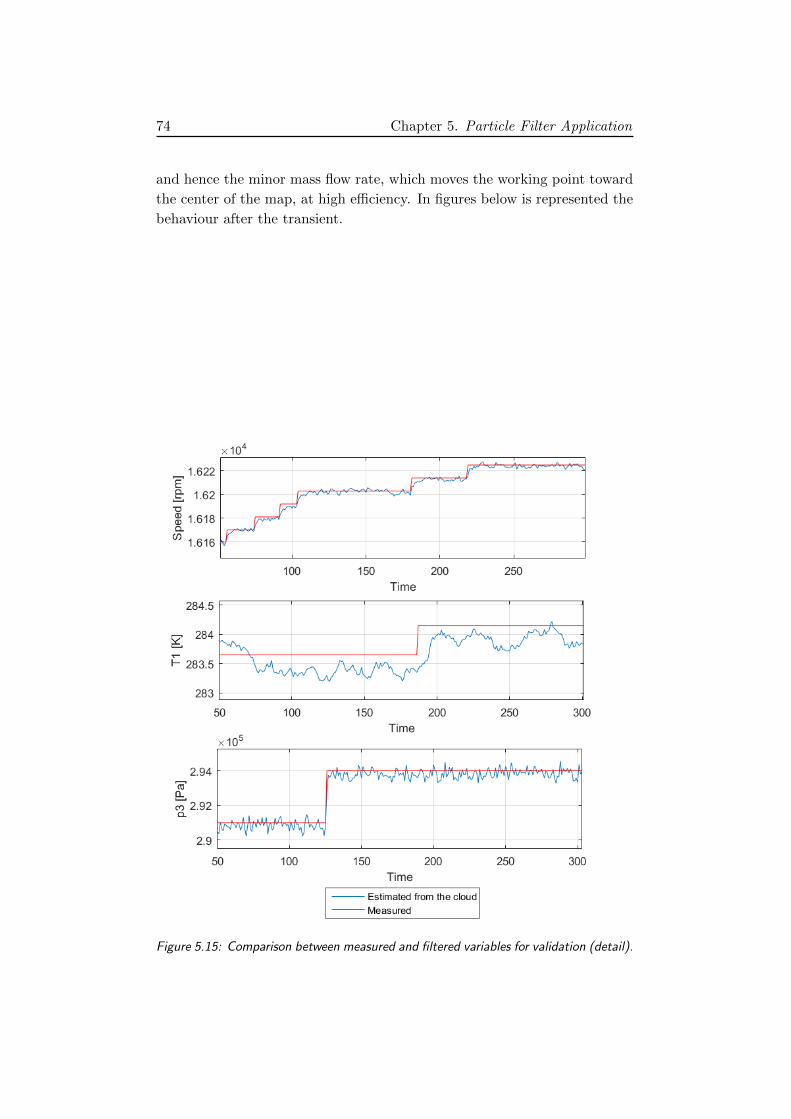
5.15 Comparison between measured and filtered variables for val-

idation (detail). . . . . . . . . . . . . . . . . . . . . . . . . . . 74

5.16 Estimation of non measured variables for validation (detail). . 75

List of Tables

3.1 Saved points for Ω = 250[s−1] . . . . . . . . . . . . . . . . . 47

5.1 Measured variables . . . . . . . . . . . . . . . . . . . . . . . . 58

5.2 Normalized percent eigenvalues for different data blocks . . . 62

C.1 Impeller geometry for validation . . . . . . . . . . . . . . . . 92

C.2 Vaneless diffuser geometry for validation . . . . . . . . . . . . 92

C.3 Vaned diffuser geometry for validation . . . . . . . . . . . . . 93

C.4 Volute geometry for validation . . . . . . . . . . . . . . . . . 93

ix

Chapter 1

Introduction

A turbocharger is a turbine-driven forced induction device that increases

an internal combustion engine’s efficiency and power output by forcing ex-

tra air into the combustion chamber [17]. More in general, a supercharger

is a mechanical device whose purpose is to increase the inlet air density,

or charge, of an internal combustion engine. The idea dates back to last

years of the nineteenth century, when combustion engine pioneers Diesel

and Daimler recognized the advantage of compressing inlet air of cylinders.

The first publication was yet released in 1905 by Buchi, in which the idea

of drive a turbine with the engine exhaust gases to power the compressor

was shown; however the idea was complex and not followed immediately

by a practical realization. The first commercial turbocharged diesel engine

appeared in 1924, after years of development leaded by Buchi, his employer

Sulzer Brothers and Brown-Boveri & Co. Ltd. The second World War was

the impetus to major developments in engines and turbomachinery, conse-

quently promoting the spreading of turbochargers. In the following years

more and more engines were turbocharged, and turbocharging was even in-

troduced in power generation and locomotive applications. To see turbo also

in automotive market was necessary to wait until 1970’s, when the oil crisis

and increasing stringent emission tresholds forced the industry to turn to

turbocharging. Nowadays, turbocharging finds application even in areas like

spark ignition engines and fuel cells, and non-turbocharged Diesel engines

are nearly obsolete.

1.1 Operation principles of turbochargers

The introduction of air into an engine cylinder at a density greater than

ambient allows a proportional increase of the fuel that can be burnt, thereby

1

2 Chapter 1. Introduction

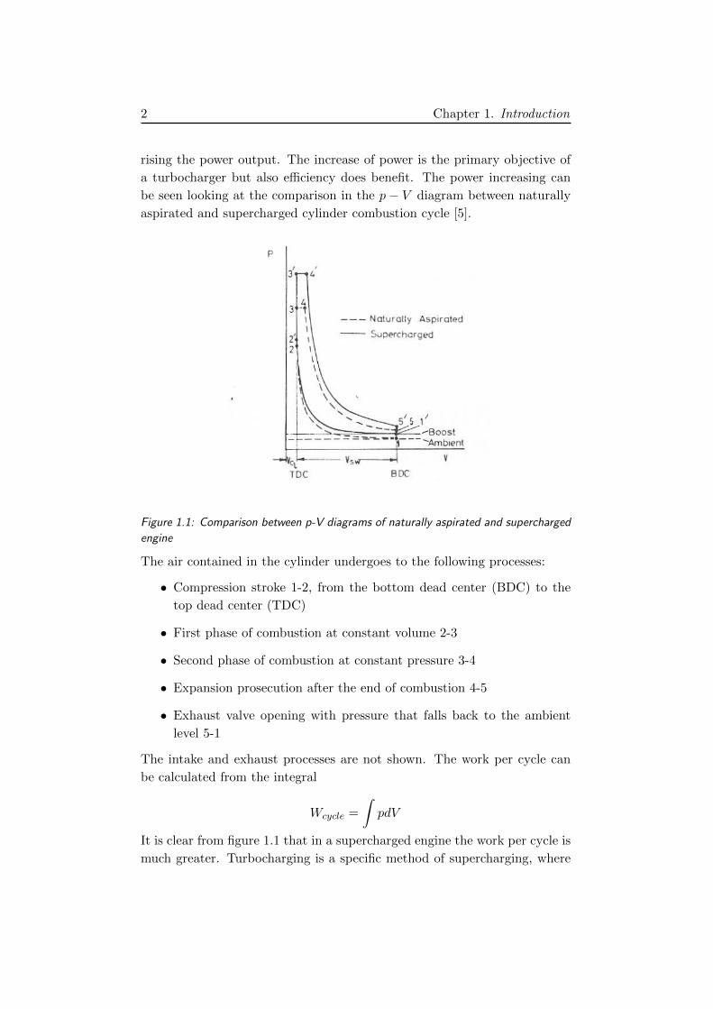
rising the power output. The increase of power is the primary objective of

a turbocharger but also efficiency does benefit. The power increasing can

be seen looking at the comparison in the p− V diagram between naturally

aspirated and supercharged cylinder combustion cycle [5].

Figure 1.1: Comparison between p-V diagrams of naturally aspirated and supercharged

engine

The air contained in the cylinder undergoes to the following processes:

• Compression stroke 1-2, from the bottom dead center (BDC) to the

top dead center (TDC)

• First phase of combustion at constant volume 2-3

• Second phase of combustion at constant pressure 3-4

• Expansion prosecution after the end of combustion 4-5

• Exhaust valve opening with pressure that falls back to the ambient

level 5-1

The intake and exhaust processes are not shown. The work per cycle can

be calculated from the integral

Wcycle =

∫pdV

It is clear from figure 1.1 that in a supercharged engine the work per cycle is

much greater. Turbocharging is a specific method of supercharging, where

Chapter 1. Introduction 3

energy contained in the exhaust gases of the engine is employed to drive a

gas turbine, which in turn drives a centrifugal compressor to feed the engine

cylinders.

1.2 Turbocharger structure

The main components of a turbocharger are the following:

• Compressor

• Turbine

• Charge cooler

• Center housing hub rotating assembly (CHRA)

• Filter/Silencer

Figure 1.2: ABB turbocharger structure

The compressor is almost universally of the radial outflow type (i.e. cen-

trifugal). Nowadays it is preferred to the axial one because of its convenient

combination of delivered pressure ratio, size and production costs.

The turbine is usually radial in compact and low power applications, such

as in automotive field. For high power application in general a single stage

axial turbine is preferred.

The charge cooler aim is to further increase the air density after the com-

pression. In fact the compression is accompanied by a temperature rise, and

looking at the perfect gas law


ρ =p

RT

it is possible to notice that a decrease in temperature causes an increase

in density, permitting then to send more mass of air in the cylinders and

to burn more fuel per cycle. Across the cooler there is a pressure drop,

which however is not relevant and do not undermines the utility of such

device. Usually an air-to-water heat exchanger is employed, and since it is

positioned between the compressor and the engine the device often it takes

the name of intercooler.

The CHRA is the structure in which the shaft connecting compressor and

turbine, the bearings and the lubricating/cooling systems are contained.

The silencer is necessary because of the huge amount of noise produced by

the compressor side, which insulating material cannot absorb completely.

It acts also as a filter for the air and for this reason it is mounted before

the compressor intake. Its operation is based on the principle of sound

absorption, sound waves arising in the compressor are reflected and damped.

1.3 Types of turbocharging

1.3.1 Constant pressure turbocharging

In this configuration, that was the first developed, gases exiting from the

engine cylinders are damped in a large exhaust manifold in order to deliver

a steady flow to the turbine. In fact turbines work better with steady flows,

while the gas coming from cylinders is inherently unstable, then damping

them in a large chamber makes the turbine work at higher efficiency.

1.3.2 Pulse system turbocharging

The disadvantage of the constant pressure system is that the high kinetic

energy of gases leaving the engine is not employed by the turbine. The

pulse system by contrary connects the engine with the turbine by means

of short narrow exhaust manifolds, making possible the transfer of kinetic

energy in form of pressure waves. As already said the flow leaving the

engine is highly unsteady, so that to ensure a correct energy recovery by the

turbine a shrewdness must be implemented, that is connecting the narrow

exhaust pipes from several cylinders in order to obtain an average overall

steady turbine flow. This method is in general preferable since it increases

available energy and turbine efficiency, but has the cons of a more difficult

design.


1.4 Problem statement and motivation

1.4.1 Case study: Marseglia generation plant

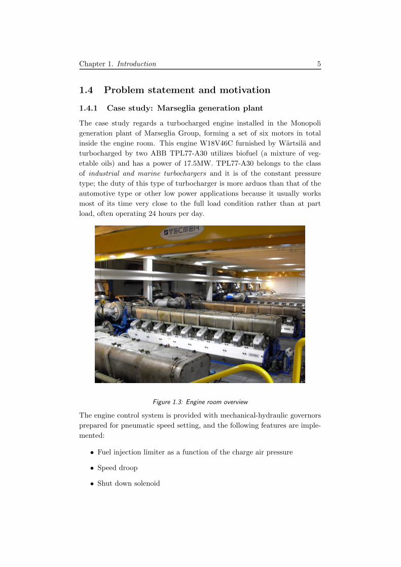
The case study regards a turbocharged engine installed in the Monopoli

generation plant of Marseglia Group, forming a set of six motors in total

inside the engine room. This engine W18V46C furnished by Wartsila and

turbocharged by two ABB TPL77-A30 utilizes biofuel (a mixture of veg-

etable oils) and has a power of 17.5MW. TPL77-A30 belongs to the class

of industrial and marine turbochargers and it is of the constant pressure

type; the duty of this type of turbocharger is more arduos than that of the

automotive type or other low power applications because it usually works

most of its time very close to the full load condition rather than at part

load, often operating 24 hours per day.

Figure 1.3: Engine room overview

The engine control system is provided with mechanical-hydraulic governors

prepared for pneumatic speed setting, and the following features are imple-

mented:

• Fuel injection limiter as a function of the charge air pressure

• Speed droop

• Shut down solenoid


The present work is most oriented on identification and monitoring on tur-

bochargers’ variables, using the engine features as boundary conditions for

the problem. For this reason the engine control system will not be taken in

consideration, making the assumption that the turbocharged engine is well

controlled.

1.4.2 Monitoring system

In a turbocharged Diesel engine, the turbocharger performance is very criti-

cal in the overall system: a 1% decrease of turbocharger performance corre-

sponds about to a 5% decrease of the engine performance. The turbocharger

efficiency can be calculated with the following expression [4] [6]

ηTC = ηmηT ηc (1.1)

where:

• ηm mechanical efficiency at the shaft

• ηT turbine efficiency

• ηc compressor efficiency

The major losses in a turbocharger occur in the compressor, rather than

in the turbine or at the shaft, making the estimation of the compressor

efficiency a fundamental point for the monitoring system. This estimation

algorithm will be incorporated in the supervision unit of the engine control

loop:

Figure 1.4: Turbocharged engine control loop


1.4.3 Sensoring layout

In figure 1.5 it is shown what should be the layout of sensors in the tur-

bocharged engine; actually the turbochargers are two, let us call them A

and B. Each turbocharger is equipped with a magnetic pick-up measuring

the rotational speed, plus temperature and pressure sensors located in dif-

ferent points of the engine. In the specific case, not all of these sensors are

mounted; in particular, only the following measures are available:

• Speed of both turbochargers A and B

• Temperatures at compressors inlet A and B

• Temperature and pressure at the engine inlet manifold

• Temperatures before and after the turbines

The unavailability of some sensors is due to critical issues typical of these

type of installations, which discourages the employment of the full layout of

figure 1.5. For example, while in process compressors the flow rate is usually

measured, in turbochargers great vibrations take place making the place-

ment of a sensor very difficult. The same problem arise when talking about

pressure and temperature ratio, which need to be located is safe points, far

enough from vibration, impervious zones or points subject to fouling. It is

then clear how arises the necessity to estimate the non-measured variables

to keep monitored the working points of the 4 turbomachines involved in

the plant, in particular their efficiencies. For each of them, centrifugal com-

pressors in particular, efficiency should always be close to the optimal one

in order to minimize the losses, maximize the supercharging of the engine

and consequently maximizing the power production.


Figure 1.5: Sensoring layout

1.5 Structure of the thesis

This Master’s thesis is composed of two main parts. In the first a physical

model for the centrifugal compressor is developed, validated and applied to

analyze some typical loss mechanisms of this machine. In the second part,

the theory of Particle Filtering is presented and applied together with the

model to optimally estimate some non-measured variables in the compressor.

In detail, chapters are organized in the following way:

• Chapter 1 introduces the topic of turbochargers, describing the struc-

ture and the operation principles. Next an introduction to the problem

is presented, together with the description of the case study plant.

• Chapter 2 treats the theory and the philosophy for centrifugal com-

pressors modelling. The notions of loss and efficiency are introduced,

with a description of most common kinds of losses.

• Chapter 3 provides the validation of the physical model and shows

how it can be applied to infer the flow conditions and to analyze some

of the losses described in the previous chapter.


• Chapter 4 introduces to Bayesian inference problem and presents in

detail the theory of non-linear Particle Filtering.

• Chapter 5 shows how the analysis of the available experimental data

was performed. Next, it describes how the Particle Filter can be ap-

plied to optimally estimate non measured variables in turbocharger’s

compressor and turbine.

• Chapter 6 outlines the conclusions of the work and proposes possible

future perspectives and enhancements.

• Appendix A introduces fundamental equations of thermodynamics and

fluid mechanics, on which the compressor modelling theory is based.

• Appendix B provides some notions of probability theory and statistics,

introductory to the non-linear Bayesian filtering.

• Appendix C furnishes the data set used for the validation of the com-

pressor model.

Chapter 2

Centrifugal Compressor

Modelling

In commercial turbochargers, the charging device universally adopted is the

centrifugal compressor. With respect to the axial compressor, it is more

compact, efficient, inexpensive and rotates at very high speed so that it

can be directly coupled to the gas turbine. The charging device has the

task to deliver to the inlet manifold of the engine a suitable boost pressure,

greater than the atmospheric one. Centrifugal compressor carries out this

task by whirling the fluid outward, thereby rising its angular momentum

and consequently, as will be seen, increasing its pressure and density.

2.1 Motivation for physical compressor modelling

Usually in industrial applications, variables such as fluid temperatures, pres-

sures and flow rates (from which the compressor behaviour, stability and

efficiency can be monitored) are measured only at the compressor inlet and

outlet, almost nothing can then be deduced about what is happening inside

the compressor and in each component. Physical modelling permits to work

out this problem, allowing to build a procedure with which the trend of

internal compressor variables and efficiencies in different sections can be in-

ferred. In the turbochargers field, compressor modelling has a primary role

in the overall turbocharged engine simulator. It finds application even in

the design phase of centrifugal compressors, where a performance prediction

procedure is necessary to ensure that the designed geometry is suitable for

a future correct operation of the machine or to compare and assess some

possible optimizations of mechanical features.

Compressor modelling can be faced in different manners. Typically the

11

12 Chapter 2. Centrifugal Compressor Modelling

physical modelling strategies are distinguished in three main categories, de-

pending on the number of dimensions in which the analysis is carried out:

• 0D-1D modelling, that use the fundamental equations of the ther-

modynamics and other first engineering principles, where the chosen

coordinate is the principal direction of the fluid.

• 2-dimensional modelling.

• 3-dimensional modelling, realized by means of CFD.

Computational FluidDynamics is obviously the most accurate and physically

reliable modelling technique, but often the huge required computational

effort discourages its employment in favour of a simplified and almost equally

reliable 1D modelling.

2.1.1 1D Modelling

In this work the one-dimensional modelling technique is used. It comprises

a mix of one-dimensional gas thermodynamics, empirical flow models and

loss correlations, used to analyze the gas flow process across the different

components of the centrifugal compressor. The procedure consists, as will

be seen in detail, in separately considering the compressor’s components

and to calculate for each of them the discharge conditions from available

inlet conditions, and then to use the former as inlet conditions in the next

component.

2.2 Compressor structure

The centrifugal compressor is constituted by stationary and dynamic com-

ponents. Usually it is modelled as the series of 5 elements:

• The compressor intake (inlet section 0 - outlet section 1), that is the

converging duct in which the fluid is drawn and axially directed toward

the eye of the impeller; in some applications, at its end inlet guided

vanes are mounted in order to minimize dynamically the incidence loss

at impeller inlet.

• The impeller (1-2), the rotating part where the work is transferred

from the blades to the fluid; the initial part is called inducer and its

function is to smoothly draw the entering distorted flow and to provide

as uniform a flow profile as possible. The surface closest to the axis

of rotation is called hub, while the shroud is the farthest. Usually in

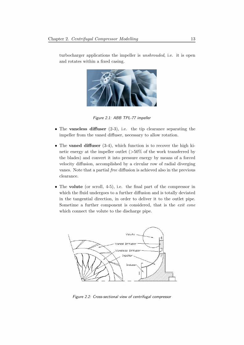
Chapter 2. Centrifugal Compressor Modelling 13

turbocharger applications the impeller is unshrouded, i.e. it is open

and rotates within a fixed casing.

Figure 2.1: ABB TPL-77 impeller

• The vaneless diffuser (2-3), i.e. the tip clearance separating the

impeller from the vaned diffuser, necessary to allow rotation.

• The vaned diffuser (3-4), which function is to recover the high ki-

netic energy at the impeller outlet (>50% of the work transferred by

the blades) and convert it into pressure energy by means of a forced

velocity diffusion, accomplished by a circular row of radial diverging

vanes. Note that a partial free diffusion is achieved also in the previous

clearance.

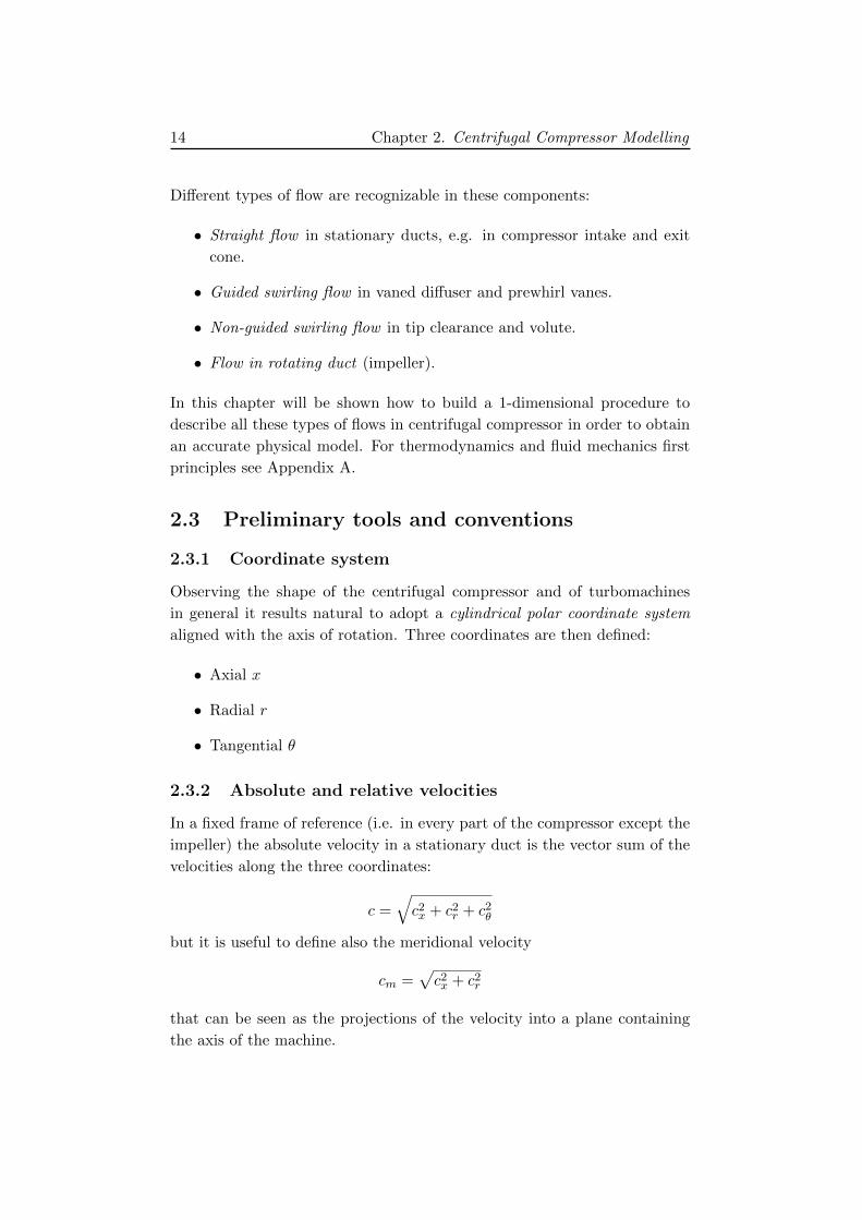
• The volute (or scroll, 4-5), i.e. the final part of the compressor in

which the fluid undergoes to a further diffusion and is totally deviated

in the tangential direction, in order to deliver it to the outlet pipe.

Sometime a further component is considered, that is the exit cone

which connect the volute to the discharge pipe.

Figure 2.2: Cross-sectional view of centrifugal compressor


Different types of flow are recognizable in these components:

• Straight flow in stationary ducts, e.g. in compressor intake and exit

cone.

• Guided swirling flow in vaned diffuser and prewhirl vanes.

• Non-guided swirling flow in tip clearance and volute.

• Flow in rotating duct (impeller).

In this chapter will be shown how to build a 1-dimensional procedure to

describe all these types of flows in centrifugal compressor in order to obtain

an accurate physical model. For thermodynamics and fluid mechanics first

principles see Appendix A.

2.3 Preliminary tools and conventions

2.3.1 Coordinate system

Observing the shape of the centrifugal compressor and of turbomachines

in general it results natural to adopt a cylindrical polar coordinate system

aligned with the axis of rotation. Three coordinates are then defined:

• Axial x

• Radial r

• Tangential θ

2.3.2 Absolute and relative velocities

In a fixed frame of reference (i.e. in every part of the compressor except the

impeller) the absolute velocity in a stationary duct is the vector sum of the

velocities along the three coordinates:

c =√c2x + c2

r + c2θ

but it is useful to define also the meridional velocity

cm =√c2x + c2

r

that can be seen as the projections of the velocity into a plane containing

the axis of the machine.


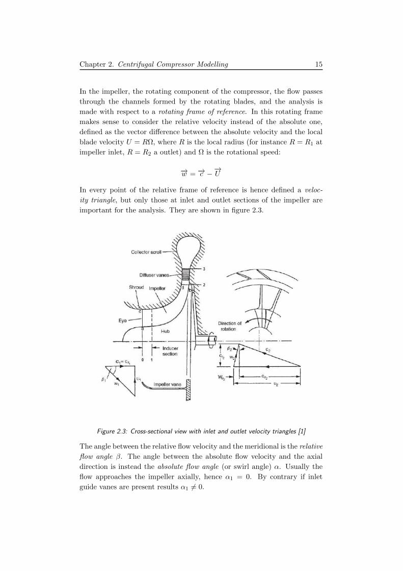
In the impeller, the rotating component of the compressor, the flow passes

through the channels formed by the rotating blades, and the analysis is

made with respect to a rotating frame of reference. In this rotating frame

makes sense to consider the relative velocity instead of the absolute one,

defined as the vector difference between the absolute velocity and the local

blade velocity U = RΩ, where R is the local radius (for instance R = R1 at

impeller inlet, R = R2 a outlet) and Ω is the rotational speed:

−→w = −→c −−→U

In every point of the relative frame of reference is hence defined a veloc-

ity triangle, but only those at inlet and outlet sections of the impeller are

important for the analysis. They are shown in figure 2.3.

Figure 2.3: Cross-sectional view with inlet and outlet velocity triangles [1]

The angle between the relative flow velocity and the meridional is the relative

flow angle β. The angle between the absolute flow velocity and the axial

direction is instead the absolute flow angle (or swirl angle) α. Usually the

flow approaches the impeller axially, hence α1 = 0. By contrary if inlet

guide vanes are present results α1 6= 0.


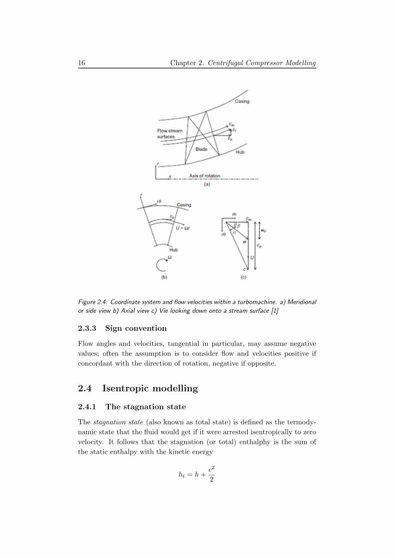
Figure 2.4: Coordinate system and flow velocities within a turbomachine. a) Meridional

or side view b) Axial view c) Vie looking down onto a stream surface [1]

2.3.3 Sign convention

Flow angles and velocities, tangential in particular, may assume negative

values; often the assumption is to consider flow and velocities positive if

concordant with the direction of rotation, negative if opposite.

2.4 Isentropic modelling

2.4.1 The stagnation state

The stagnation state (also known as total state) is defined as the termody-

namic state that the fluid would get if it were arrested isentropically to zero

velocity. It follows that the stagnation (or total) enthalphy is the sum of

the static enthalpy with the kinetic energy

ht = h+c2

2


In centrifugal compressors it is usually considered h = cpT , where cp is the

specific heat at constant pressure. Hence the stagnation temperature, or

total temperature, can be expressed as

Tt = T +c2

2cp

Recalling now the relationships linking the specific heats and the isentropic

exponent γ (appendix A), cp can be expressed as

cp =γR

γ − 1

Then we have

Tt = T(

1 +γ − 1

2

c2

γRT

)Introducing the Mach number, as the ratio between the local absolute ve-

locity and the velocity of sound

M =c

cso=

c√γRT

(2.1)

we obtain finally the expression of the stagnation temperature as a function

of the static temperature and Mach number only

Tt = T(

1 +γ − 1

2M2)

(2.2)

The definition of stagnation pressure and density is straightforward (see

appendix A):

pt = p(

1 +γ − 1

2M2) γγ−1

(2.3)

ρt = ρ(

1 +γ − 1

2M2) 1γ−1

(2.4)

In the rotating frame of reference it is defined also the relative Mach number

M ′ =w√γRT

(2.5)

The first law of thermodynamics for turbomachines treating gas is usu-

ally expressed in the following form

Pcm

= ht2 − ht1 (2.6)


where Pcm is the power absorbed by the compressor per unit of mass flow rate.

It can be observed that if the work transfer to or from the fluid is zero, as

happens in stationary ducts, the stagnation enthalpy and consequently the

stagnation temperature is constant, no care if the flow is isentropic or not.

We will refer to this property as stagnation enthalpy conservation. If the

flow is even isentropic, the stagnation pressure and density are also constant.

2.4.2 The relative stagnation state and Rothalpy

In the impeller the work transfer is different from zero, then it is necessary

to find a property similar to total enthalpy that is conserved through the

flow path. Defining the relative stagnation enthalpy as the sum of the static

enthalpy with the relative kinetic energy

h′t = h+w2

2(2.7)

it is possible to demonstrate that the quantity that remains constant across

the impeller is the so called rothalpy, which is defined as

I = h′t −U2

2= cpT +

w2

2− U2

2= constant (2.8)

2.4.3 Adimensional Mass Flow Rate Equation

In this section the fundamental adimensional mass flow rate equation, on

which the solving procedure of each duct is based, is derived and discussed.

From now on we will refer to it as AME.

We start from the continuity equation m = ρcA.

Using the (2.1) and the perfect gas law:

m

A=

p

RTM√γRT

Now invert the stagnation relationships (2.2)(2.3) and substitute to p and

T . Rearranging, the first form of the AME is obtained:

m√

RTtγ

Apt= M

(1 +

γ − 1

2M2)− γ+1

2(γ−1)(2.9)

The term on the left hand side is a function of the mass flow, flow area and

stagnation state; the right hand side is instead a function f(M) of the Mach

number only, having the shape of figure 2.5.

As can be observed, ifM < 1 the function has a behaviour such that it can be

solved for the Mach number, usually iteratively with the Newton-Raphson


Figure 2.5: AME diagram

method (about 4-5 steps to convergence). When the flow reaches the sonic

speed (M = 1) at the minimum flow area of the flow path (throat) it is

said to be choked and the mass flow rate cannot further increase. In choked

flow conditions, depending on the geometry of the compressor, subsonic or

supersonic speed flow may occur in some section of the compressor; having

the AME two solutions (a subsonic and a supersonic one), the correct one

must be chosen accordingly, observing that a supersonic flow (M > 1) can

only be achieved in an expanding area downstream of the throat.

2.4.4 Use AME to calculate fluid flow process

Consider the compressor intake, i.e. the converging duct previous to the

impeller, with inlet and outlet sections respectively 0 and 1. Suppose it is

adiabatic and isentropic: then Tt and pt are constant along the duct and

equal to the respective inlet stagnation conditions, which are supposed to

be known (usually the atmospheric ones)

Tt = Tt0 pt = pt0

Equation (2.9) holds in every point of the duct, in particular at the outlet

section, thus the Mach number at the outlet M1 can be calculated by solving

iteratively:

m√

RTt0γ

A1pt0= M1

(1 +

γ − 1

2M2

1

)− γ+12(γ−1)


We’ve done this for the compressor intake but the same procedure is adopted

for any duct.

If the considered component for which we want to solve the flow process is

the impeller (namely inlet section 1 and outlet section 2), we have to replace

absolute quantities with relative ones:

m√

RT ′t2γ

A2p′t1= M ′2

(1 +

γ − 1

2M ′22

)− γ+12(γ−1)

(2.10)

But now the relative stagnation temperature is no more constant and the

equation to solve must be slightly modified. From (2.8) the following relation

between inlet and outlet relative enthalpies holds:

h′t2 − h′t1 =1

2(U2

2 − U21 ) (2.11)

from which the relation between inlet and outlet relative stagnation tem-

peratures is obtained:

T ′t2 = T ′t1 +1

2cp(U2

2 − U21 ) (2.12)

Substituting in (2.10), results that for the impeller AME has to be solved

in the following form:

m√

RT ′t1γ

A2p′t1= M2

(1 +

γ − 1

2M2

2

)− γ+12(γ−1)

(1− U2

1 − U22

2cpT ′t1

) γ+12(γ−1)

(2.13)

2.4.5 Slip factor

Suppose that impeller is of the backward swept blades type, i.e. with blades

exit angle opposite to the direction of rotation. This is in general a preferable

configuration with respect to the purely radial blades configuration because

it allows to reduce the Mach number at impeller exit, then making difficult

to reach the choking condition in vaned diffuser throat. If the flow at the

impeller outlet were perfectly guided by the blades, the following relations

would hold:

cθ2 = U2 + cm2 tanβB2

where βB2 is the exit geometric blade angle of impeller.

But because of the finite number of blades, the flow it is said to slip, with

the effect of modifying the exit velocity triangle and leading to a smaller

tangential velocity cθ2 , hence reducing the delivered pressure ratio. Note


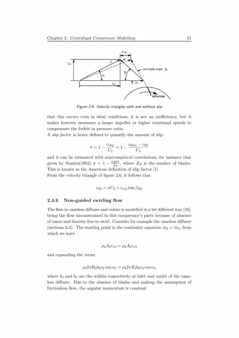
Figure 2.6: Velocity triangles with and without slip

that this occurs even in ideal conditions, it is not an inefficiency, but it

makes however necessary a larger impeller or higher rotational speeds to

compensate the forfeit in pressure ratio.

A slip factor is hence defined to quantify the amount of slip:

σ = 1−cslipU2

= 1− cθ2∞ − cθ2U2

and it can be estimated with semi-empirical correlations, for instance that

given by Stanitz(1952) σ = 1 − 0.63πZB

, where ZB is the number of blades.

This is known as the American definition of slip factor [1].

From the velocity triangle of figure 2.6, it follows that

cθ2 = σU2 + cm2 tanβB2

2.4.6 Non-guided swirling flow

The flow in vaneless diffuser and volute is modelled in a bit different way [16],

being the flow unconstrained in this compressor’s parts because of absence

of vanes and thereby free to swirl. Consider for example the vaneless diffuser

(sections 2-3). The starting point is the continuity equation m2 = m3, from

which we have

ρ2A2cr2 = ρ3A3cr3

and expanding the terms

ρ22πR2b2c2 cosα2 = ρ32πR3b3c3 cosα3

where b2 and b3 are the widths respectively at inlet and outlet of the vane-

less diffuser. Due to the absence of blades and making the assumption of

frictionless flow, the angular momentum is constant


R2cθ2 = R3cθ3

Combining the two previous equations, under the further assumption of

parallel walled vaneless diffuser (b2 = b3) we have

tanα2

ρ2=

tanα3

ρ3(2.14)

The exit absolute flow angle can be found iteratively, initially giving a rea-

sonable value to ρ3 and iterating until converging. Then c3 can be calculated

from the continuity equation and T3 from stagnation temperature conserva-

tion.

2.5 Compressor losses

The work transfer in actual conditions is always less than the ideal work, due

to dissipation phenomena involved in the fluid process. In this section, first

the compressor efficiency will be defined, then the main loss mechanisms

will be introduced showing later how flow equations modifies to take losses

into account.

2.5.1 Compressor efficiency

The compressor efficiency is defined in the following intuitive form:

ηc :=work input in ideal process

actual work input

but to avoid confusion we have to define it more clearly. In particular, this

definition of efficiency requires to specify 3 items:

• the inlet and outlet states, if static or stagnation.

• the reference ideal process.

• whether external (or parasitic) losses are included or not.

Inlet and exit states

Usually to compute efficiency the stagnation state is chosen as inlet state

because also the kinetic energy has a role in the compressor dynamics. The

exit state is by contrast more arguable, but the following criterion is usually

adopted:


• if the outlet kinetic energy can be used in some way, stagnation state

is chosen.

• if the exit kinetic energy is almost completely wasted, exit static pres-

sure is adopted.

The latter could be the case of turbocharger’s compressors, where the exit

kinetic energy is very little used, only to partially aid scavenging (i.e. the

stroke period in which discharge gases are ejected from the engine cylinders).

The ideal process

The isentropic (or adiabatic) process is almost always considered as reference

ideal process. As already discussed, the work transfer per unit of mass flow

equals the change in total enthalpy. Considering for example the impeller:

Pcm

= ht2 − ht1

The total-to-total efficiency expression takes then the following form:

ηtt =ht2s − ht1ht2 − ht1

Figure 2.7: Mollier diagram for compression process in the impeller


But this expression is unusable because the state 2s does not have a real

physical meaning; then substituting the total enthalpy with the total tem-

perature (i.e. simplifying cp) and using the thermodynamic relationship

Tt2Tt1

= (pt2pt1

)γ−1γ

the total-to-total efficiency results in:

ηtt =(pt2pt1 )

γ−1γ − 1

Tt2Tt1− 1

being pt2 = pt2s.

Likewise, the static-to-static efficiency is:

ηss =(p2

p1)γ−1γ − 1

T2T1− 1

(2.15)

Under the assumption that the inlet and the exit velocities are similar,

follows that ηtt ' ηss. The other isentropic efficiency commonly used is the

total-to-static, defined as

ηts =( p2

pt1)γ−1γ − 1

Tt2Tt1− 1

External losses

External losses, or parasitic losses, are associated with losses originating

from minor flows leaking away from the main flow through the compressor;

they account for mechanisms such as the recirculation at the eye of the

impeller and leakage through the space between the shroud and the casing.

Parasitic losses produce an enthalpy rise without any change in the pressure

ratio, so the choice to include them or not in the compressor efficiency is

arbitrary. Usually in turbocharger applications they are supposed to be part

of the turbine losses.

2.5.2 Physics of loss mechanisms

In this work 11 different types of losses has been considered:

• Skin friction loss: the loss generating from the contact of the fluid

with the blades or duct surface.


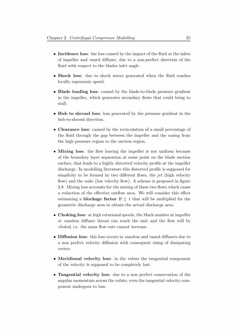
• Incidence loss: the loss caused by the impact of the fluid at the inlets

of impeller and vaned diffuser, due to a non-perfect direction of the

fluid with respect to the blades inlet angle.

• Shock loss: due to shock waves generated when the fluid reaches

locally supersonic speed.

• Blade loading loss: caused by the blade-to-blade pressure gradient

in the impeller, which generates secondary flows that could bring to

stall.

• Hub to shroud loss: loss generated by the pressure gradient in the

hub-to-shroud direction.

• Clearance loss: caused by the recirculation of a small percentage of

the fluid through the gap between the impeller and the casing from

the high pressure region to the suction region.

• Mixing loss: the flow leaving the impeller is not uniform because

of the boundary layer separation at some point on the blade suction

surface, that leads to a highly distorted velocity profile at the impeller

discharge. In modelling literature this distorted profile is supposed for

simplicity to be formed by two different flows, the jet (high velocity

flow) and the wake (low velocity flow). A scheme is proposed in figure

2.8. Mixing loss accounts for the mixing of these two flows which cause

a reduction of the effective outflow area. We will consider this effect

estimating a blockage factor B ≤ 1 that will be multiplied for the

geometric discharge area to obtain the actual discharge area.

• Choking loss: at high rotational speeds, the Mach number at impeller

or vaneless diffuser throat can reach the unit and the flow will be

choked, i.e. the mass flow rate cannot increase.

• Diffusion loss: this loss occurs in vaneless and vaned diffusers due to

a non perfect velocity diffusion with consequent rising of dissipating

vortex.

• Meridional velocity loss: in the volute the tangential component

of the velocity is supposed to be completely lost.

• Tangential velocity loss: due to a non perfect conservation of the

angular momentum across the volute, even the tangential velocity com-

ponent undergoes to loss.


Figure 2.8: Jet and wake velocity profiles at impeller discharge

2.5.3 Loss coefficients

As we have seen, losses in centrifugal compressor are several and acting with

very different mechanisms, making any attempt to describe all of them with

a detailed mathematical analysis incredibly difficult.

The historical and standard approach in centrifugal compressors modelling

and analysis is to calculate the isentropic flow with the equations previously

introduced and later correct the results in order to take into consideration

the effect of the losses.

This can be done by the definition of loss coefficients, one for each type of loss

mechanism, calculable by means of semi-empirical correlations which give

an estimation of the entropy change ∆s in the flow process. These empirical

correlations are the result of the accumulation of many years’ experience by

designers and researchers. It must be clear that a loss coefficient is basically

a device used to simplify the computing of actual conditions, therefore it

has only a limited physical validity; if it had an exact physical validity it

would become integral part of the model.

In order to be able to compare different types of losses, a common defini-

tion of loss coefficient is necessary. We will use the static enthalpy loss

coefficient, defined as

ξ =∆hy12c

2y

(2.16)

where with y we have indicated the exit section of the generic duct for which

the loss coefficient has to be computed. ∆hy = hy − hys is the enthalpy


difference between the isentropic-isobaric (ideal) case and the actual case:

loss coefficients aim is then to estimate this enthalpy difference, normalized

with respect to the outlet isentropic kinetic energy. For example, a loss

coefficient to model skin friction loss was suggested by Aungier (1995):

ξsf = 4Cfw2

c22

LBDH

where Cf is the impeller skin friction coefficient, depending on the impeller

construction material, w = w1+w22 , LB the mean camberline length of im-

peller blades, DH the hydraulic diameter of impeller channels. Observe that

loss coefficients depend on:

• Inlet and discharge isentropic conditions of the considered duct (e.g.

w1 and w2).

• Geometry of the considered duct.

this means that they are calculable only after that isentropic conditions have

been found.

It is possible to demonstrate [2] that the isentropic AME in presence of losses

simply modifies in:

• For stators:

m√

RTt0γ

A1pt0= e−

∆sR M1

(1 +

γ − 1

2M2

1

)− γ+12(γ−1)

(2.17)

• For impeller (1-2):

m√

RT ′t1γ

A2p′t1= e−

∆sR M2

(1 +

γ − 1

2M2

2

)− γ+12(γ−1)

(1− U2

1 − U22

2cpT ′t1

) γ+12(γ−1)

(2.18)

where the term e−∆sR includes the effect of entropy variation ∆s due to

losses, for simplicity of notation let us call it µ. This term is computable

once the loss coefficients have been obtained by means of the empirical cor-

relations. For the static enthalpy loss coefficient it is possible to demonstrate

the following relation:

µ =(

1 +γ − 1

2ξovM

22

) γγ−1

(2.19)

where ξov is the overall loss coefficient, obtained summing all coefficients of

each loss mechanism.


2.6 Model structure

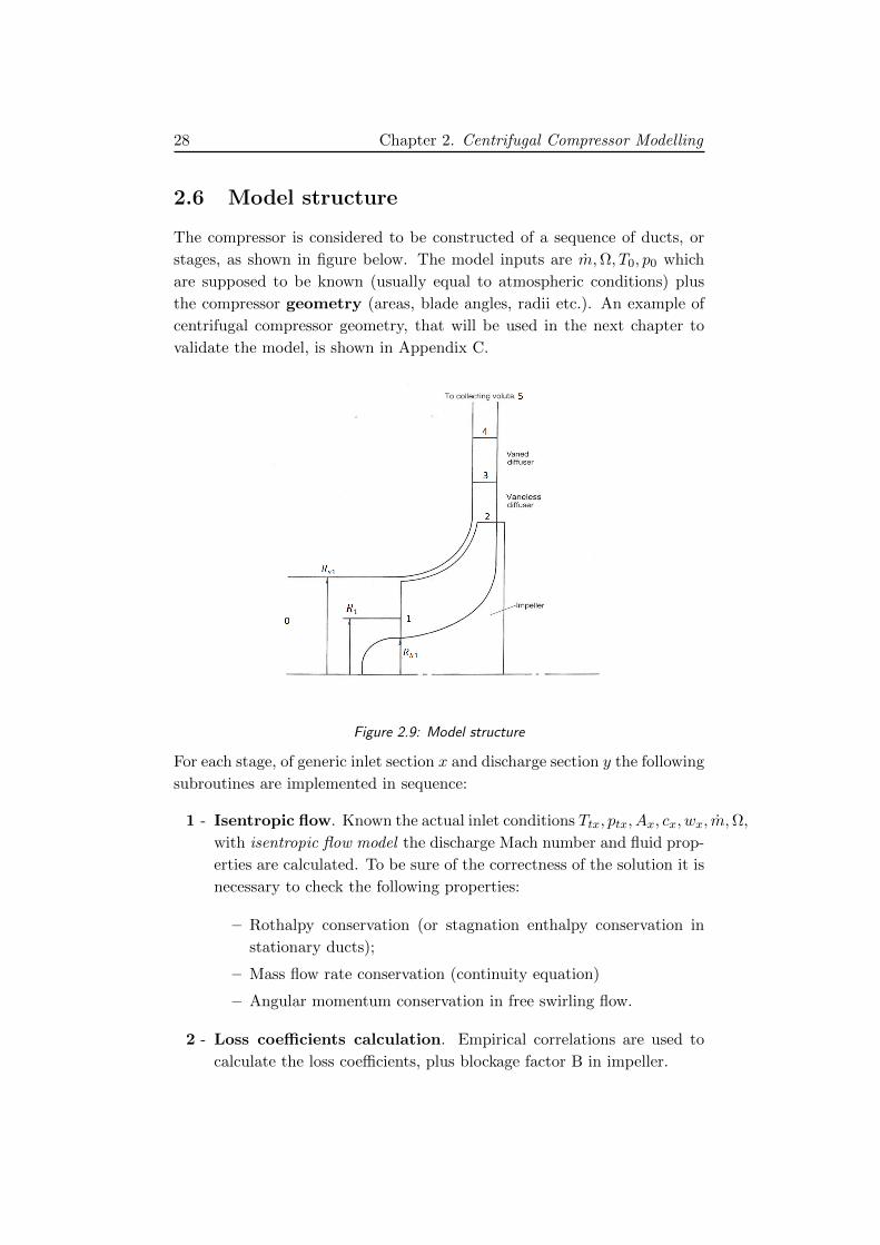
The compressor is considered to be constructed of a sequence of ducts, or

stages, as shown in figure below. The model inputs are m,Ω, T0, p0 which

are supposed to be known (usually equal to atmospheric conditions) plus

the compressor geometry (areas, blade angles, radii etc.). An example of

centrifugal compressor geometry, that will be used in the next chapter to

validate the model, is shown in Appendix C.

Figure 2.9: Model structure

For each stage, of generic inlet section x and discharge section y the following

subroutines are implemented in sequence:

1 - Isentropic flow. Known the actual inlet conditions Ttx, ptx, Ax, cx, wx, m,Ω,

with isentropic flow model the discharge Mach number and fluid prop-

erties are calculated. To be sure of the correctness of the solution it is

necessary to check the following properties:

– Rothalpy conservation (or stagnation enthalpy conservation in

stationary ducts);

– Mass flow rate conservation (continuity equation)

– Angular momentum conservation in free swirling flow.

2 - Loss coefficients calculation. Empirical correlations are used to

calculate the loss coefficients, plus blockage factor B in impeller.


3 - Correction step. Loss coefficients are employed to correct the ideal

discharge conditions found in step 1 and obtain the actual onesMy, py, Ty, Ay, cy, wy.

Again a check of mass and rothalpy/stagnation enthalpy conservation

is required.

4 - Proceed to next duct. The actual discharge quantities calculated

are the input of the next duct and the procedure is repeated from step

1.

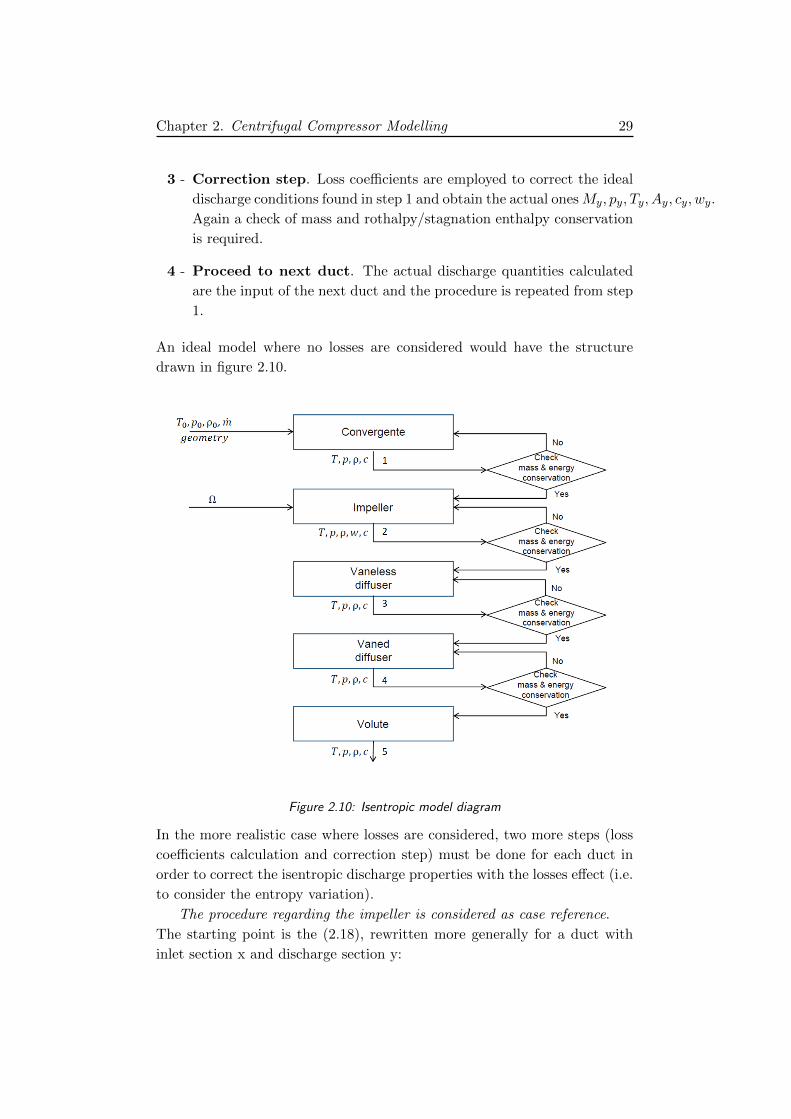
An ideal model where no losses are considered would have the structure

drawn in figure 2.10.

Figure 2.10: Isentropic model diagram

In the more realistic case where losses are considered, two more steps (loss

coefficients calculation and correction step) must be done for each duct in

order to correct the isentropic discharge properties with the losses effect (i.e.

to consider the entropy variation).

The procedure regarding the impeller is considered as case reference.

The starting point is the (2.18), rewritten more generally for a duct with

inlet section x and discharge section y:


m√

RT ′txγ

Ayp′tx= µMy

(1 +

γ − 1

2M2y

)− γ+12(γ−1)

(1−

U2x − U2

y

2cpT ′tx

) γ+12(γ−1)

(2.20)

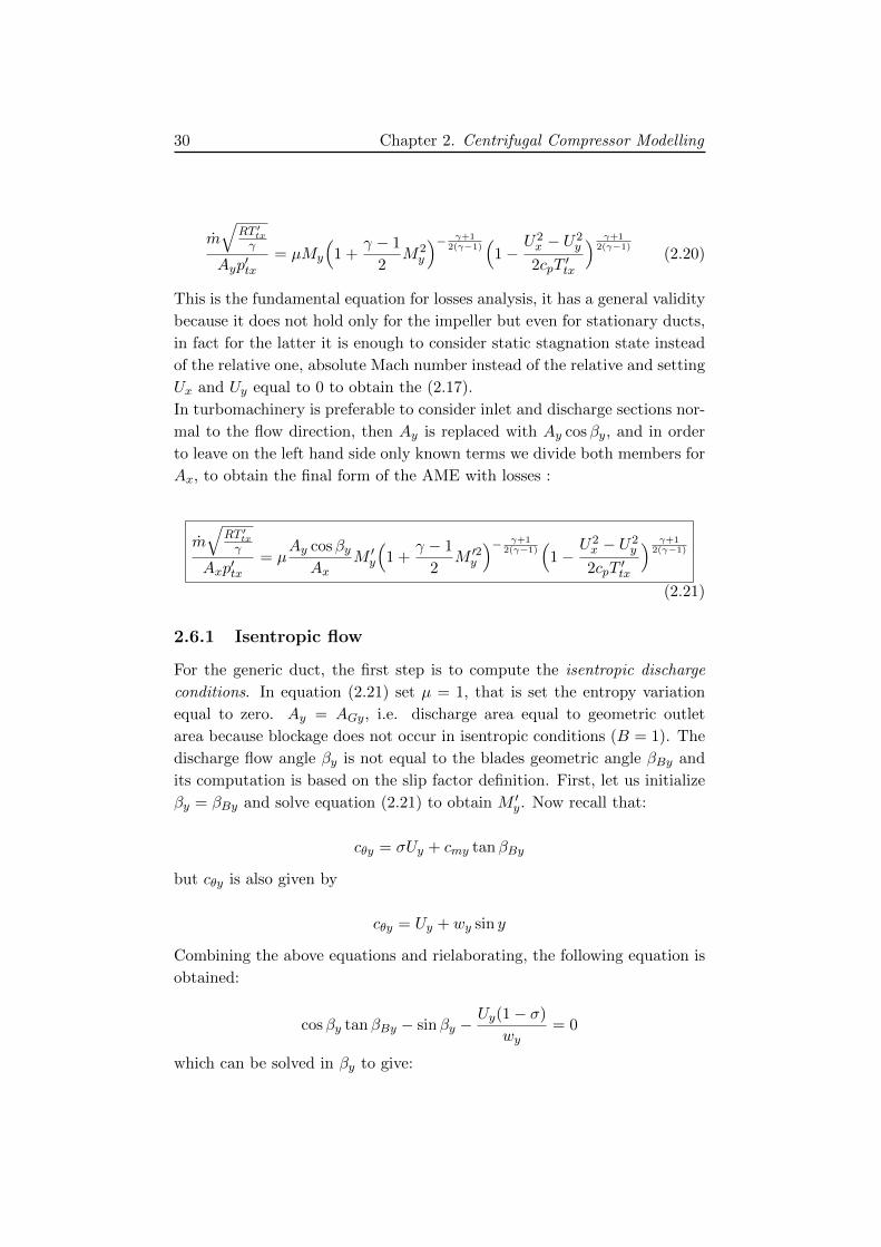
This is the fundamental equation for losses analysis, it has a general validity

because it does not hold only for the impeller but even for stationary ducts,

in fact for the latter it is enough to consider static stagnation state instead

of the relative one, absolute Mach number instead of the relative and setting

Ux and Uy equal to 0 to obtain the (2.17).

In turbomachinery is preferable to consider inlet and discharge sections nor-

mal to the flow direction, then Ay is replaced with Ay cosβy, and in order

to leave on the left hand side only known terms we divide both members for

Ax, to obtain the final form of the AME with losses :

m√

RT ′txγ

Axp′tx= µ

Ay cosβyAx

M ′y

(1 +

γ − 1

2M ′2y

)− γ+12(γ−1)

(1−

U2x − U2

y

2cpT ′tx

) γ+12(γ−1)

(2.21)

2.6.1 Isentropic flow

For the generic duct, the first step is to compute the isentropic discharge

conditions. In equation (2.21) set µ = 1, that is set the entropy variation

equal to zero. Ay = AGy, i.e. discharge area equal to geometric outlet

area because blockage does not occur in isentropic conditions (B = 1). The

discharge flow angle βy is not equal to the blades geometric angle βBy and

its computation is based on the slip factor definition. First, let us initialize

βy = βBy and solve equation (2.21) to obtain M ′y. Now recall that:

cθy = σUy + cmy tanβBy

but cθy is also given by

cθy = Uy + wy sin y

Combining the above equations and rielaborating, the following equation is

obtained:

cosβy tanβBy − sinβy −Uy(1− σ)

wy= 0

which can be solved in βy to give:


sinβy =

−Uy(1−σ)wy

+ tanβBy

√1 + tan2βBy −

U2y (1−σ)2

w2y

1 + tan2βBy

wy is eliminated inverting the (2.5) and using (2.2)

wy = M ′y

√γRT ′ty

1 + γ−12 M ′2y

where T ′ty is obtained from the rothalpy conservation:

T ′ty = T ′tx +1

2cp(U2

y − U2x)

The procedure is repeated recursively until the converging of M ′y and βy.

The computation of remaining isentropic discharge quantities is straightfor-

ward.

Ty =T ′ty

1 + γ−12 M ′2y

wy =M ′y√γRTy

cmy = wy cosβy

cθy = Uy + cmy tanβy

cy =√c2my + c2

θy

αy = atancθycmy

My =cy√γRTy

p′ty = p′tx(T ′tyT ′tx

)

γγ−1

µ

p′y =p′ty

1 + γ−12 M ′2y

η =(pypx

)γ−1γ − 1

TyTx− 1

Finally, it is suggested to verify at the end of each subroutine the following

fundamental properties, that the computed quantities must satisfy:


• Rothalpy conservation in impeller

cpTx +w2x

2− U2

x

2= cpTy +

w2y

2−U2y

2

or stagnation enthalpy conservation in stators

cpTx +c2x

2= cpTy +

c2y

2

• Mass flow conservation (continuity equation)

ρxcxAnx = ρycyAny

where with An we indicate the area normal to the flow direction.

• Perfect gas law relation between py, Ty, ρy

2.6.2 Loss coefficients calculations

The second step is the evaluation of the effect of losses, for which it is nec-

essary to compute a set of loss coefficients ξi, every one of which depends

on the respective loss mechanism, geometry of the compressor and the isen-

tropic inlet and discharge properties of the considered duct. An overall loss

coefficient is finally given by the sum of all loss coefficients:

ξov = ξsf + ξinc + ξsl + ξbl + ξhs + ...

from which the value of parameter µ is computed using the (2.19).

Moreover, blockage factor B is estimated with a correlation, for example that

suggested by Aungier [3]. This permits to estimate the actual discharge flow

area as Ay = BAGy.

2.6.3 Correction step for actual flow

The proceeding to obtain the actual discharge conditions is the same of

the isentropic flow, but now using the value of µ computed in the previous

section and also considering the reduction of the impeller discharge area due

to mixing of flows by means of the blockage factor B. AME is solved again

iteratively to find the actual discharge properties of the considered duct.

These will be the input properties of the next duct in the flow path. The

correction step for a single duct is outlined in the diagram of figure 2.11.


Figure 2.11: Scheme for actual flow computation

Chapter 3

Model Validation and Losses

Analysis

3.1 Compressor map

The compressor map is a chart representing the compressor behaviour in

terms of pressure ratio and efficiency with respect to flow rate and rotational

speed. It is usually obtained by compressor rig test, but it can be seen

also as a graphical representation of the model described in the previous

chapter. A finite number of rotational speeds are chosen (usually 10-15, from

the minimum to the maximum allowed) and for each of them the pressure

ratio across the machine is plotted as a function of the volumetric flow;

in addition curves of isoefficiency may be plotted. The function returning

the temperature ratio is not plotted but it can be simply derived inverting

the (2.15). At low volumetric flow, each curve terminates at the surge line;

beyond this line, the so-called surge phenomenon takes place and the process

becomes unstable. At high volumetric flows speed curves become more and

more steep because of the choking phenomenon (Mach number across the

section of minimum flow area tends to 1 and the mass flow cannot increase

further).

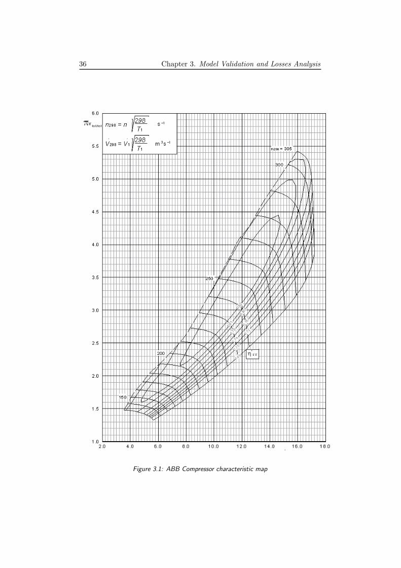
The ABB turbocharger’s compressor map of the case study, obtained during

the turbomachine testing, is shown in Fig. 3.1. The more the map plotted by

the model will be similar to the experimental map, the more the model will

be reliable. The map inputs are Ω298 (or n298 as indicated in the document)

and V298 , i.e. rotational speed [s−1] and the flow rate at ISO conditions

[m3/s]. At different inlet temperature T1, the inputs are calculated with the

following conversion formulas Ω298 = Ω√

298T1

, V298 = V1

√298T1

.

35

36 Chapter 3. Model Validation and Losses Analysis

Figure 3.1: ABB Compressor characteristic map

Chapter 3. Model Validation and Losses Analysis 37

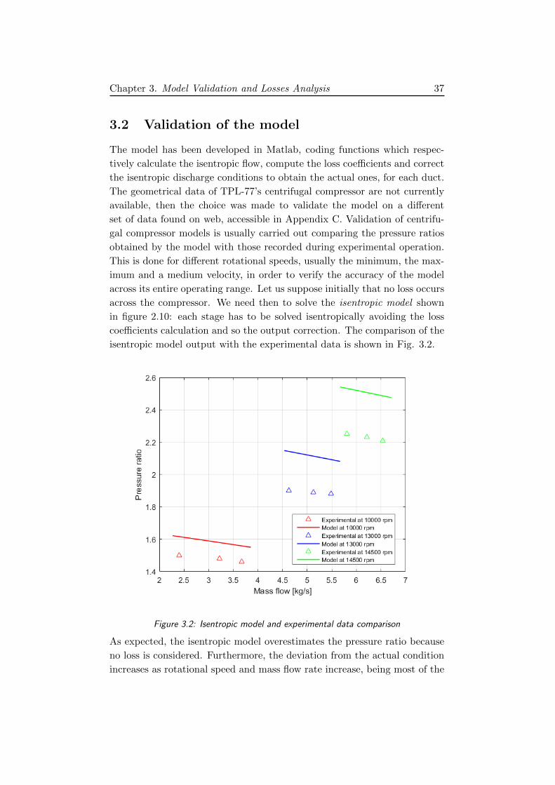
3.2 Validation of the model

The model has been developed in Matlab, coding functions which respec-

tively calculate the isentropic flow, compute the loss coefficients and correct

the isentropic discharge conditions to obtain the actual ones, for each duct.

The geometrical data of TPL-77’s centrifugal compressor are not currently

available, then the choice was made to validate the model on a different

set of data found on web, accessible in Appendix C. Validation of centrifu-

gal compressor models is usually carried out comparing the pressure ratios

obtained by the model with those recorded during experimental operation.

This is done for different rotational speeds, usually the minimum, the max-

imum and a medium velocity, in order to verify the accuracy of the model

across its entire operating range. Let us suppose initially that no loss occurs

across the compressor. We need then to solve the isentropic model shown

in figure 2.10: each stage has to be solved isentropically avoiding the loss

coefficients calculation and so the output correction. The comparison of the

isentropic model output with the experimental data is shown in Fig. 3.2.

Figure 3.2: Isentropic model and experimental data comparison

As expected, the isentropic model overestimates the pressure ratio because

no loss is considered. Furthermore, the deviation from the actual condition

increases as rotational speed and mass flow rate increase, being most of the


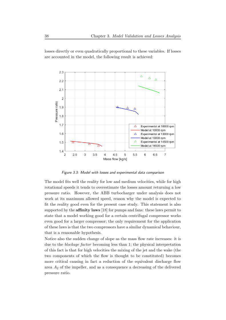
losses directly or even quadratically proportional to these variables. If losses

are accounted in the model, the following result is achieved:

Figure 3.3: Model with losses and experimental data comparison

The model fits well the reality for low and medium velocities, while for high

rotational speeds it tends to overestimate the losses amount returning a low

pressure ratio. However, the ABB turbocharger under analysis does not

work at its maximum allowed speed, reason why the model is expected to

fit the reality good even for the present case study. This statement is also

supported by the affinity laws [18] for pumps and fans: these laws permit to

state that a model working good for a certain centrifugal compressor works

even good for a larger compressor; the only requirement for the application

of these laws is that the two compressors have a similar dynamical behaviour,

that is a reasonable hypothesis.

Notice also the sudden change of slope as the mass flow rate increases: it is

due to the blockage factor becoming less than 1; the physical interpretation

of this fact is that for high velocities the mixing of the jet and the wake (the

two components of which the flow is thought to be constituted) becomes

more critical causing in fact a reduction of the equivalent discharge flow

area A2 of the impeller, and as a consequence a decreasing of the delivered

pressure ratio.


3.3 Geometrical parameters identification

Once the model is validated it can be applied to the case study turbocharger’s

compressor to analyse its performance in each stage or to simply get the de-

livered pressure and temperature ratios. As already said the compressor

geometry is currently unknown and the number of geometrical parameters

involved in the model (including also those participating in the losses em-

pirical correlations) is very high, making any attempt to identify all of them

from the provided experimental compressor map pointless. The most fun-

damental parameter, that one who determines the size and hence the power

of the centrifugal compressor is the impeller exit radius R2. Then the choice

was made to identify only the impeller exit radius and assigning reasonable

values to the other parameters, according to standard values furnished by

literature. The identification is operated on the map of figure 3.1. Two

points are chosen from the compressor map, on the same velocity curve

Ω = 290 [s−1] and with same efficiency η = 0.81. Suppose that compressor

inlet conditions are the atmospheric ones p0 = pat, T0 = Tat, ρ0 = ρat, it is

then possible to extract the pressure ratio rp and the volumetric flow V .

Point A Point B

V 14.4 15.8 [m3/s]

rp 4.6 4.8

From the definition of efficiency (2.15), the outlet temperature (section 5,

volute outlet) is computed for both points:

T5 = T0

(1 +

rγ−1γ

p − 1

η

)Then p5 is computed from the pressure ratio and the density from the perfect

gas law:

p5 = rpp0 ρ5 =ρ5

RT5

Using the Euler’s turbomachine equation (appendix A), and considering that

the compressor power can also be expressed as the enthalpy change across

the machine, we have:

mcp(T5 − T0) = m(U22 − U2w2 sinβ2)

The relative velocity at impeller exit can be expressed as


w2 =m

ρ2A2 cosβ2

Supposing β2 = 45 and ρ2 = 2.5[kg/m3] for both points A and B, we obtain

the following system of two equations in 2 unknownsmAcp(T5A − T0) = mA((R2Ω)2 −R2Ω mA

ρ2A2tanβ2)

mBcp(T5B − T0) = mB((R2Ω)2 −R2Ω mBρ2A2

tanβ2)

which solution is

R2 = 0.271[m] A2 = 0.087[m2]

The remaining parameters are chosen opportunely scaling those used in the

validation and assuming typical blade angles suggested by literature.

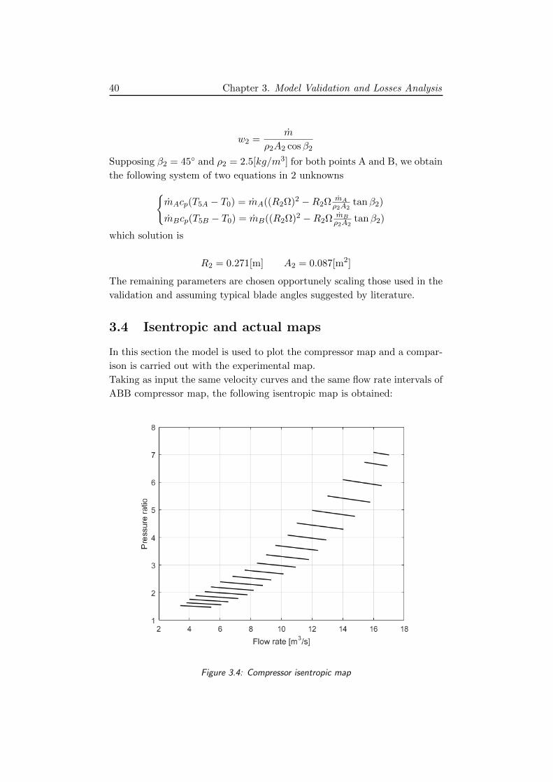
3.4 Isentropic and actual maps

In this section the model is used to plot the compressor map and a compar-

ison is carried out with the experimental map.

Taking as input the same velocity curves and the same flow rate intervals of

ABB compressor map, the following isentropic map is obtained:

Figure 3.4: Compressor isentropic map


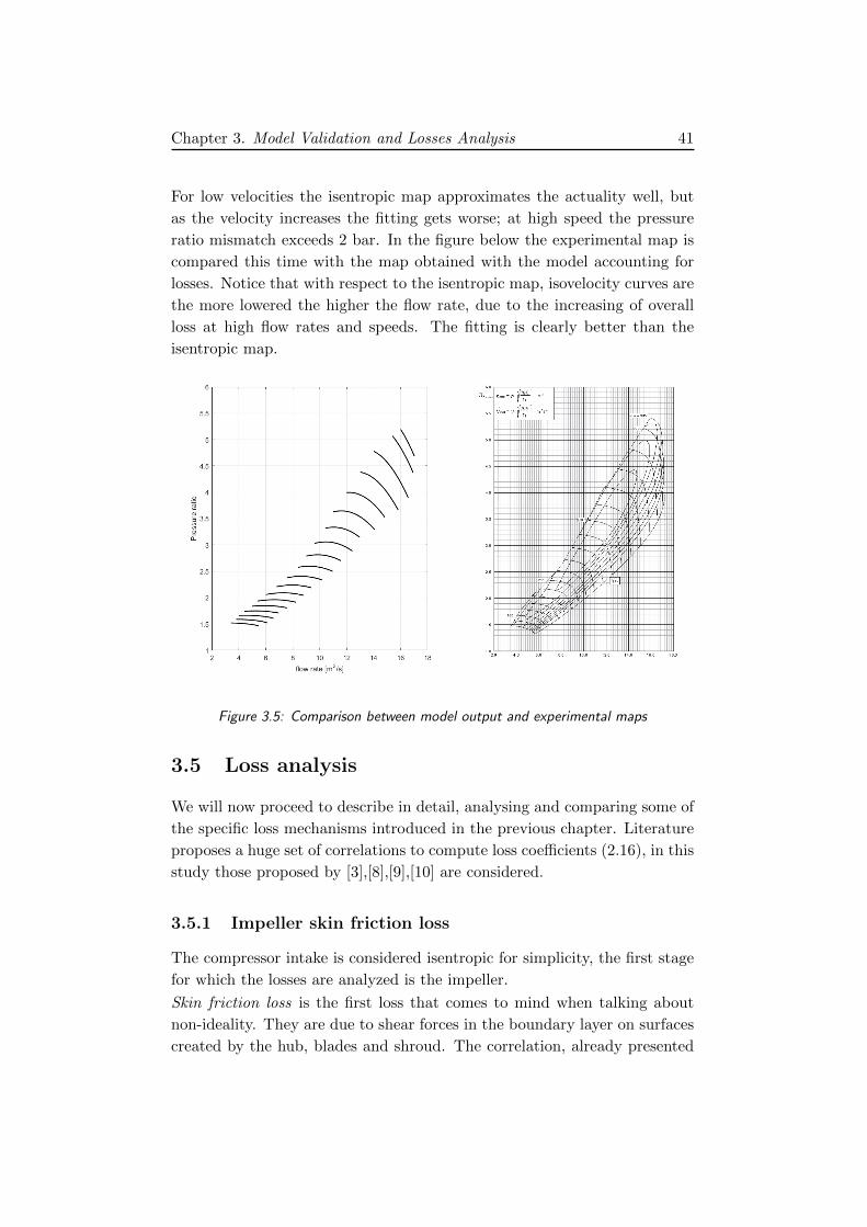
For low velocities the isentropic map approximates the actuality well, but

as the velocity increases the fitting gets worse; at high speed the pressure

ratio mismatch exceeds 2 bar. In the figure below the experimental map is

compared this time with the map obtained with the model accounting for

losses. Notice that with respect to the isentropic map, isovelocity curves are

the more lowered the higher the flow rate, due to the increasing of overall

loss at high flow rates and speeds. The fitting is clearly better than the

isentropic map.

Figure 3.5: Comparison between model output and experimental maps

3.5 Loss analysis

We will now proceed to describe in detail, analysing and comparing some of

the specific loss mechanisms introduced in the previous chapter. Literature

proposes a huge set of correlations to compute loss coefficients (2.16), in this

study those proposed by [3],[8],[9],[10] are considered.

3.5.1 Impeller skin friction loss

The compressor intake is considered isentropic for simplicity, the first stage

for which the losses are analyzed is the impeller.

Skin friction loss is the first loss that comes to mind when talking about

non-ideality. They are due to shear forces in the boundary layer on surfaces

created by the hub, blades and shroud. The correlation, already presented


in the previous chapter. assumes that the loss is equivalent to that suffered

by a fully developed flow in a pipe of circular cross section:

ξsf = 4Cfw2

c22

LBDH

where

• Cf impeller skin friction coefficient

• LB mean camberline length of impeller blades

• DH impeller channels hydraulic diameter

• w = w1+w22 average relative velocity

• c2 absolute flow velocity at impeller outlet

The skin friction coefficient Cf depends on the construction material of the

impeller and on the flow conditions of the boundary layer, if turbulent or

laminar. Usually it is estimated with approximated formulas depending on

the Reynolds number. In this study we set Cf = 10−3.

The hydraulic diameter DH is a parameter commonly used when treating

flows in non-circular channels, and it is defined as DH = 4Aper , where A is the

cross-section area and per the wetted perimeter. In impeller it is estimated

again with empirical correlations, such as that suggested in [8].

As already said at each loss is associated an increase of entropy. The overall

entropy entropy increase ∆s can be calculated recalling that µ = e−∆sR as:

∆s = −R logµ

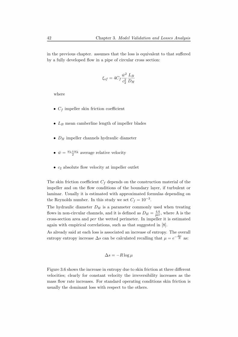
Figure 3.6 shows the increase in entropy due to skin friction at three different

velocities; clearly for constant velocity the irreversibility increases as the

mass flow rate increases. For standard operating conditions skin friction is

usually the dominant loss with respect to the others.


Figure 3.6: Entropy variation due to skin friction loss for different rotational speeds

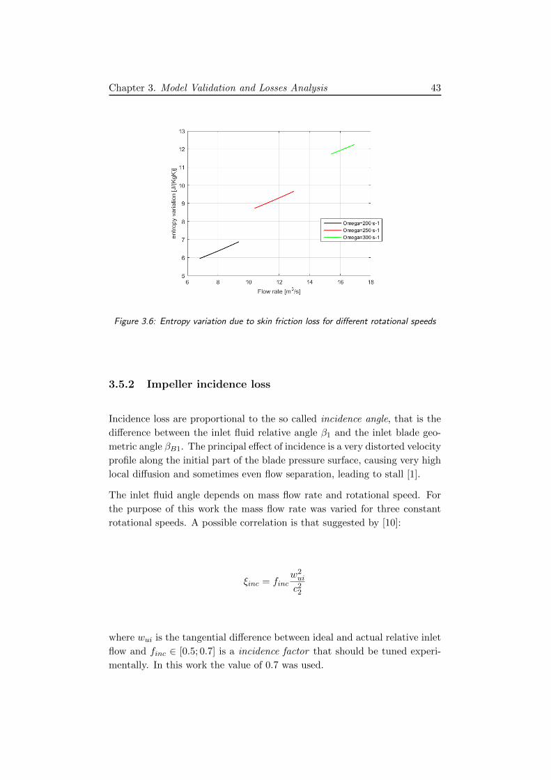
3.5.2 Impeller incidence loss

Incidence loss are proportional to the so called incidence angle, that is the

difference between the inlet fluid relative angle β1 and the inlet blade geo-

metric angle βB1. The principal effect of incidence is a very distorted velocity

profile along the initial part of the blade pressure surface, causing very high

local diffusion and sometimes even flow separation, leading to stall [1].

The inlet fluid angle depends on mass flow rate and rotational speed. For

the purpose of this work the mass flow rate was varied for three constant

rotational speeds. A possible correlation is that suggested by [10]:

ξinc = fincw2ui

c22

where wui is the tangential difference between ideal and actual relative inlet

flow and finc ∈ [0.5; 0.7] is a incidence factor that should be tuned experi-

mentally. In this work the value of 0.7 was used.


Figure 3.7: Entropy variation due to incidence loss for different rotational speeds

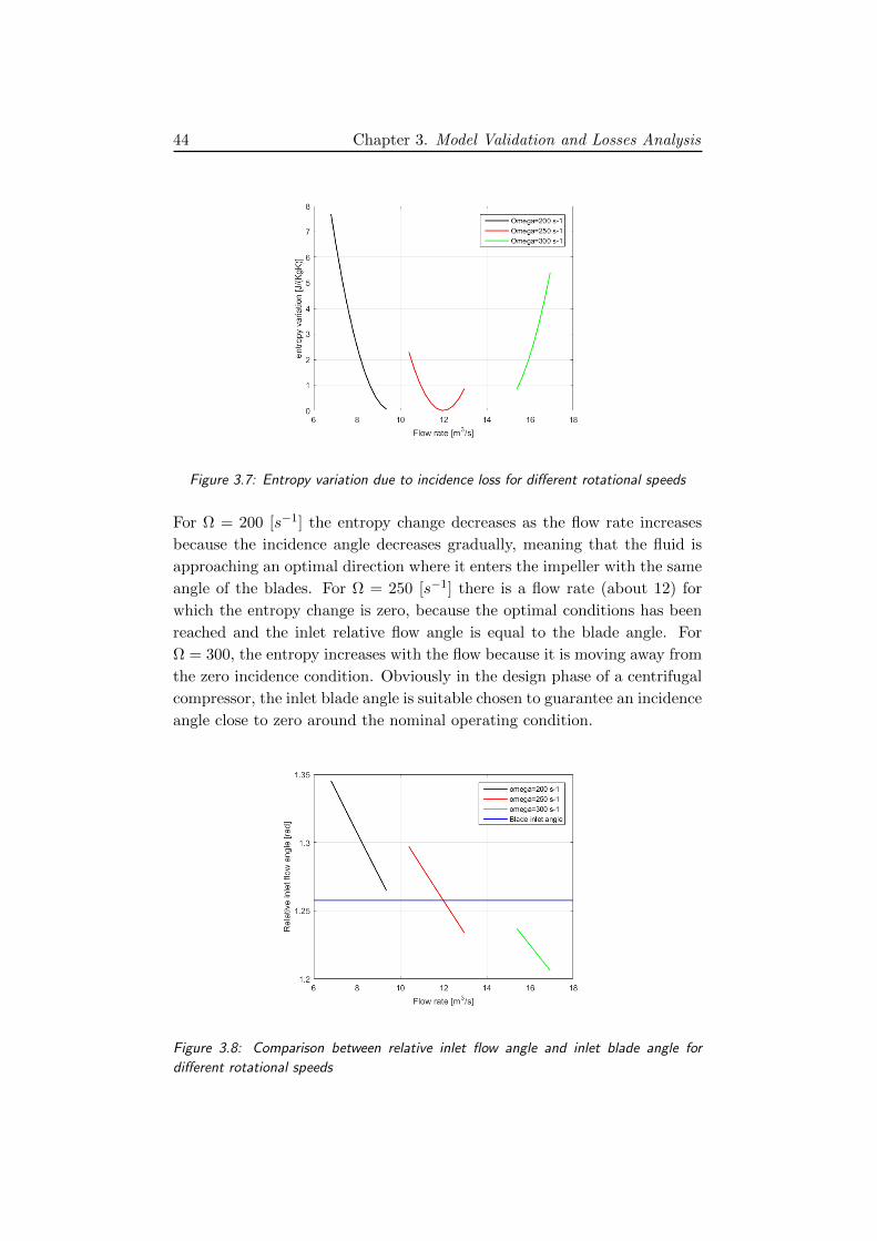
For Ω = 200 [s−1] the entropy change decreases as the flow rate increases

because the incidence angle decreases gradually, meaning that the fluid is

approaching an optimal direction where it enters the impeller with the same

angle of the blades. For Ω = 250 [s−1] there is a flow rate (about 12) for

which the entropy change is zero, because the optimal conditions has been

reached and the inlet relative flow angle is equal to the blade angle. For

Ω = 300, the entropy increases with the flow because it is moving away from

the zero incidence condition. Obviously in the design phase of a centrifugal

compressor, the inlet blade angle is suitable chosen to guarantee an incidence

angle close to zero around the nominal operating condition.

Figure 3.8: Comparison between relative inlet flow angle and inlet blade angle for

different rotational speeds


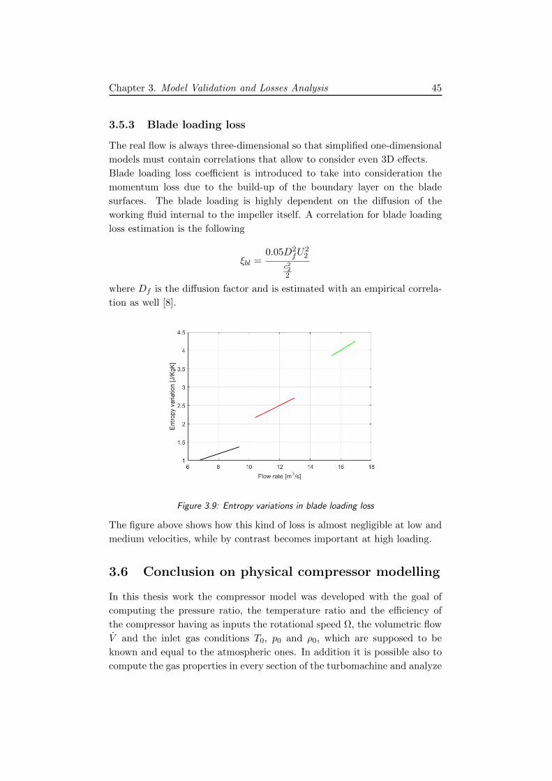
3.5.3 Blade loading loss

The real flow is always three-dimensional so that simplified one-dimensional

models must contain correlations that allow to consider even 3D effects.

Blade loading loss coefficient is introduced to take into consideration the

momentum loss due to the build-up of the boundary layer on the blade

surfaces. The blade loading is highly dependent on the diffusion of the

working fluid internal to the impeller itself. A correlation for blade loading

loss estimation is the following

ξbl =0.05D2

fU22

c222

where Df is the diffusion factor and is estimated with an empirical correla-

tion as well [8].

Figure 3.9: Entropy variations in blade loading loss

The figure above shows how this kind of loss is almost negligible at low and

medium velocities, while by contrast becomes important at high loading.

3.6 Conclusion on physical compressor modelling

In this thesis work the compressor model was developed with the goal of

computing the pressure ratio, the temperature ratio and the efficiency of

the compressor having as inputs the rotational speed Ω, the volumetric flow

V and the inlet gas conditions T0, p0 and ρ0, which are supposed to be

known and equal to the atmospheric ones. In addition it is possible also to

compute the gas properties in every section of the turbomachine and analyze


the impact of the different losses mechanisms, evaluating the efficiency of

the components individually.

The losses analysis is by the way a secondary objective of the thesis, and fur-

thermore the exact geometrical parameters are not available; for the above

reasons, from now on the model will be used as a white box like that in figure

3.10, disregarding the internal phenomena in each stage.

Figure 3.10: Compressor ”white box” model

The model returns hence as output the overall pressure and temperature

ratios rp and rT , plus the overall efficiency η (static-to-static for simplicity).

3.7 Alternative Compressor Modelling

In cases like this in which the geometrical parameters indispensable for a

correct physical modelling were not available but the experimental com-

pressor map is provided, the compressor model can be developed simply

reproducing the map by means of a suitable interpolating algorithm.

The basic idea of the algorithm is to select from the experimental map a

finite number of points, saving for each point the deductible and interested

quantities and, by interpolation, find the desired output for any input.

In the specific case, for every iso-velocity curve of the ABB map 4 points were

chosen, respectively on the surge margin, on the choke line, at maximum

efficiency and at an intermediate point between the latter two, as shown in

figure 3.11.


Figure 3.11: Chosen points for interpolation

For each of these points the value of V , rp, η can be read; the temperature

ratio is conversely computable from equation (2.15). For instance, for Ω =

250 [s−1] the points shown in table are saved:

A B C D Units

V 10.15 12 12.8 13.4 [kg/s]

rp 3.45 3.4 3.25 2.62

η 0.81 0.82 0.81 0.65

rT 1.52 1.51 1.48 1.43

Table 3.1: Saved points for Ω = 250[s−1]

The algorithm performs first an interpolation in Ω, computing the 4-points

matrix for values of Ω different from those saved; afterwards it identifies in

which of the three intervals A-B, B-C or C-D the input is and performs a

further interpolation in V to return the desired output (rp, η or rT ).


3.7.1 Results

The model is applied to plot the three functions η = f1(Ω, V ), rp = f2(Ω, V )

and rT = f3(Ω, V ), for a finite number of Ω, from 230 to 305 [s−1] (Ω < 230

are not likely to verify in such plant).

Figure 3.12: Efficiency, pressure ratio and temperature ratio functions

Chapter 4

Theory of Particle Filtering

Optimal Bayesian filtering

Optimal Bayesian filtering is a class of methods that allows to estimate

the state of a non-linear time-varying system, having noisy measurements

of some variables belonging to the state space. The term optimal refers

to statistical optimality, while Bayesian refers to the the approach used to

handle the problem, which is Bayesian inference [11].

4.1 Models and notation

Nonlinear filtering is applied to non-linear discrete-time state space models

in the form: xt+1 = f(xt, vt) vt ∼ pvt x0 ∼ px0

yt = h(xt) + et et ∼ pet

x ∈ Rn y ∈ Rm

Here t denotes the time instant, vt and et are stochastic noises respectively

on the state and on the measurement equation, with probability density

functions (pdf) pvt and pet . vt and et are independent signals, each other and

with respect to the initial conditions, px0 is a pdf that represents the initial (a

priori) knowledge about the state, before any measurement incoming. From

the state space model, it is possible to obtain the more general Markov

model: xt+1 ∼ p(xt+1|xt)yt ∼ p(yt|xt)

49

50 Chapter 4. Theory of Particle Filtering

The two pdf in the Markov model are called transition probabilities and they

are implicitly defined by the state-space equations. The Bayesian approach

in non-linear filtering consists in computing or approximating the posterior

distribution of the state given the observations; this can be done recursively

by means of the Bayes update recursion:

p(xt+1|Y t+1) =p(yt+1|xt+1)p(xt+1|Y t)∫

Rnxp(yt+1|xt+1)p(xt+1|Y t)dxt+1

(4.1)

The derivation of the 4.1 is shown in Appendix B. It is useful to introduce the

so called Markov properties, which derive from the independence assumption

made on the stochastic noises:

p(xt+1|xt, xt−1, ..., yt, yt−1, ...) = p(xt+1, xt)

p(yt|xt, xt−1, ..., yt−1, yt−2, ...) = p(yt, xt)

For simplicity in notation, sequence of values of a generic signal s till the

time instant t will be compressed in the notation St, from which follows:

p(xt+1|Xt, Y t) = p(xt+1|xt)

p(yt|Xt, Y t−1) = p(yt|xt)

4.2 Optimal estimation

Theorem 1 (Optimality of conditional expectation). The conditional ex-

pectation E(x|y) is the optimal estimator of state x given the observations

y.

Proof. The conditional expectation

E(x|y) =

∫xp(x|y)dx

is a function of the observation y only, it will be denoted with g(y). We have

to demonstrate that

xopt = g(y) = arg ming(y)

E[(x− g(y)

)2]

E[(x− g(y)

)2] = E[

(x− g(y) + g(y)− g(y)

)2] =

= E[(x− g(y)

)2] + E[

(g(y)− g(y)

)2] + 2E[

(x− g(y)

)(g(y)− g(y)

)]

Chapter 4. Theory of Particle Filtering 51

Let us expand the third term

E[(x− g(y)

)(g(y)− g(y)

)] =

∫∫ (x− g(y)

)(g(y)− g(y)

)p(x, y)dxdy

Substituting p(x, y) = p(x|y)p(y)

E[(x− g(y)

)(g(y)− g(y)

)] =

∫(g(y)− g(y))p(y)

(∫(x− g(y))p(x|y)dx

)dy

=

∫(g(y)− g(y))p(y)

(g(y)− g(y)

)= 0

Hence

E[(x− g(y))2] = E[(x− g(y))2] + E[(g(y)− g(y))2]

which is minimum when g(y) = g(y).

4.3 Particle Filter Theory

Many mathematical methods to approximate the computation of the poste-

rior distribution in the 4.1 have been studied and implemented since the mid

of 1960s, such as the well known Extended Kalman Filter, the Gaussian Sum

Filter or Grid Based Methods like the Particle Filter. The basic idea of the

Particle Filter is to approximate the various distributions that appear on the

right hand side of the Bayes update recursion with discrete distributions, in

order to be able to solve integrals in a simple way; with respect to other grid

based methods, the particle filter has the great advantage of constructing

a dynamic stochastic greed, instead of a deterministic one (such as in the

Point Mass Filter), changing in time according to the information provided

by the noisy measurements. The discrete approximation of a generic pdf

is acted by means of a cloud of points, which take the name of particles,

extracted according to the continuous pdf we want to approximate:

p(xt|Y t) ≈ p(xt|Y t) =1

N

N∑i=1

δ(xt − xt,i) (4.2)

xt,i ∼ p(xt|Y t)

where δ(·) is the Dirac Delta Function, N the number of particles, xt,i the

particle i at time instant t.

NB: The sum symbol∑

is indeed an abuse of notation, it is not a sum but

a cloud of points, a set of particles.


4.3.1 A priori distribution approximation

The first step is to approximate the a priori distribution p(xt+1|Y t) that

appears in the numerator on the right hand side of the 4.1. It is called a

priori because it describes, at a generic time instant, the knowledge about

the state distribution before the arrival of the new measurement yt+1.

At t = 0 is trivial: a set of particles is sampled from px0 which must be

known

px0 ≈ px0 =1

N

N∑i=1

δ(x0 − x0,i)

For example, suppose that the prior distribution approximation of a 2-

dimensional state has to be defined. The prior knowledge on the system

permits us to say that the two states have both a Gaussian distribution:

x1 ∼ N (10, 1) x2 ∼ N (10, 3)

Sampling N = 2000 particles, the resulting a priori cloud is the following:

Figure 4.1: Cloud of particles representing the a priori distribution px0

At a generic time instant t 6= 0, suppose that p(xt|Y t) is available from the

filtering done at the previous time instant, i.e we have a set of particles1N

∑δ(xt − xt,i). We can then approximate (see Appendix B):

p(xt+1|Y t) ≈∫p(xt+1|xt)p(xt|Y t)dxt =

=1

N

N∑i=1

∫p(xt+1|xt)δ(xt − xt,i)dxt =

1

N

N∑i=1

p(xt+1|xt,i)


This is however not yet a discrete approximation, it is indeed a mean of

continuous distributions. So we further approximate:

p(xt+1|Y t) ≈ 1

N

N∑i=1

p(xt+1|xt,i) ≈1

N

N∑i=1

δ(xt+1 − ¯xt+1,i) (4.3)

where ¯xt+1,i ∼1

N

N∑i=1

p(xt+1|xt,i)

Typically ¯xt+1,i ∼ p(xt+1|xt,i) ∀i, i.e. the transition probability is the same

for every particle. Then remembering the duality between state-space model

and Markov model:

¯xt+1,i = f(xt,i, vt,i) vt,i ∼ pvtThis is also called the time propagation step: each particle is propa-

gated to the next time step using the dynamic model in order to obtain the

approximated a priori distribution at time instant t+ 1.

4.3.2 A posteriori distribution approximation

Once the a priori distribution have been approximated with the 4.3, we can

find the a posteriori distribution p(xt+1|Y t+1) directly applying the Bayes

recursive formula 4.1:


p(yt+1|xt+1)p(xt+1|Y t)dxt+1≈

≈p(yt+1|xt+1) 1

N δ(xt+1 − ¯xt+1,i)∫p(yt+1|xt+1) 1

N δ(xt+1 − ¯xt+1,i)dxt+1=

=

∑Ni=1 p(yt+1|¯xt+1,i)δ(xt+1 − ¯xt+1,i)∑N

i=1 p(yt+1|¯xt+1,i)=

=N∑i=1

qiδ(xt+1 − ¯xt+1,i)

where

qi =p(yt+1|¯xt+1,i)∑Ni=1 p(yt+1|¯xt+1,i)

i = 1, .., N

are called normalized likelihoods and are such that∑qi = 1. In practice

they are weights assigned to each particle, representing the probability that

the corresponding particle is the state at time instant t + 1 knowing that

the last measurement has the value yt+1.


The numerator p(yt+1|¯xt+1,i) is the relative likelihood of the particle i. Sup-

posing that measures have Gaussian distribution, relative likelihoods are

computed through the expression of the multivariate conditional Gaussian

distribution:

qi =1√

(2π)m|R|exp(−[yt+1 − h(xt+1)]′R−1[yt+1 − h(xt+1)]

2

)i = 1..N

(4.4)

where R is the covariance matrix of the measurement error, which is diagonal

thanks to the noises independence assumption.

The posterior distribution p(xt+1|Y t+1) is so far approximated by a set of

weighted particles. To complete the recursion the algorithm requires to put

the a posteriori distribution in the same form of the 4.2, then a further

approximation is made:

p(xt+1|Y t+1) ≈N∑i=1

qiδ(xt+1 − ¯xt+1,i) ≈1

N

N∑i=1

δ(xt+1 − xt+1,i)

with xt+1,i ∼M∑i=1

qiδ(xt+1 − ¯xt+1,i)

which means that particles need to be resampled according to the computed

weights qi.

This is the resampling step and it is fundamental in particle filtering since

it gives the indispensable feedback carried by the measurements. A possible

resampling algorithm is the following, which is called sampling importance

resampling (SIR) and is formally justified in [15]:

• Randomly generate a real number r ∈ [0, 1].

• Sum the likelihoods progressively until the accumulated sum is greater

than r; then set xt+1,i = xt,j .

It is possible to show that the obtained distribution tends, for M → ∞, to

p(xt+1|Yt+1).

4.3.3 Conditional expectation

Having the approximation of the posterior distribution p(xt+1|Y t+1) (in form

of a cloud of particles distributed accordingly), the conditional expectation

can be computed as follows:


E[xt+1|Y t+1] =

∫xt+1p(xt+1|Y t+1)dxt+1 =

=

∫xt+1

1

N

N∑i=1

δ(xt+1 − xt+1,i)dxt+1 =

=1

N

N∑i=1

∫xt+1δ(xt+1 − xt+1,i)dxt+1 =

1

N

N∑i=1

xt+1,i

4.4 Particle Filter Algorithm summary

• System model, noises pdf and the initial a priori state pdf px0 are

given.

• For t = 0, sample N particles x0,i according to px0 ; N is a tuning

parameter, a trade-off between solution accuracy and computational

effort should be found.

• For t = 1, 2, ..

– Perform the time propagation step to obtain a priori particles ¯xt,iusing the dynamic model;

– Once the measurement yt+1 is available, compute the relative

likelihoods qi = p(yt+1|¯xt+1,i) ∀i, using the 4.4;

– Normalize the relative likelihoods qi = qi∑Nj=1 qj

;

– Resampling, i.e. compute a new set of particles xt+1,i randomly

generated on the basis of the likelihoods qi (a posteriori particles);

– Now we have a posteriori distribution, a posteriori set of particles

distributed according to p(xt+1|Y t+1); on this discrete distribu-

tion we can compute any desired statistical measure, of which the

most important is the conditional expectation:

E[xt+1|Y t+1] =1

N

N∑i=1

xt+1,i (4.5)

which is the optimal estimator.

Chapter 5

Particle Filter Application

In the next sections, the Particle Filter will be employed to optimally es-

timate termodynamic variables of turbocharger that are not measured by

the engine control system. Although the computation effort of this method

is often significant, this is not an issue for the present problem because the

time between two consecutive measurements is large and does not constitute

a bottle neck.

Note on notation

There is in this chapter an abuse of notation with respect to chapters on

centrifugal compressor modelling. So far we have indicated with integers

from 1 to 5 the internal sections of the compressor. The present chapter is by

contrast focused on the general turbocharger system, then we change point

of view and the integers from 1 to 6 will indicate the following turbocharger

sections:

• 0 Silencer/Filter inlet

• 1 Compressor inlet

• 2 Compressor discharge

• 3 Intercooler discharge/Engine inlet manifold

• 4 Engine exhaust manifold

• 5 Turbine inlet

• 6 Turbine discharge

57

58 Chapter 5. Particle Filter Application

Figure 5.1: Scheme of turbocharger sections

5.1 Data analysis

Multiple data sets from Marseglia plant were available, each one containing

the time evolution in a specific month of the variables shown in table:

Description Units

ΩA,B Rotational speed for turbochargers A, B [rpm]

T1 Compressor inlet temperature [K]

T3 Engine inlet manifold temperature [K]

p3 Engine inlet manifold pressure [Pa]

T5A,B Turbine inlet temperature for turbo A, B [K]

T6A,B Turbine outlet temperature for turbo A, B [K]

∆Tcoolant Temperature drop of the cooling water in the heat exchanger [K]

Table 5.1: Measured variables

Sometimes the rotational speed will be expressed in [rad/s] or [s−1].

The sample rate for each variable is 38 seconds. Being the turbocharger

dynamics about 0.5 seconds, the system can be considered at steady state.

The data set used for the analysis will be that of February 2015 (figure 5.2).

Chapter 5. Particle Filter Application 59

Figure 5.2: Set of measures available


5.1.1 Filtering and normalization

The monthly time series show some holes probably due to sensors malfunc-

tioning or off-scale behaviours. For example, in February the measured

rotational speed goes to zero several times as can be observed from figure

5.3, clearly a sensor failure.

Figure 5.3: Unfiltered rotational speed ΩA [rpm]

For this reason a preliminary signal filtering was performed in order to obtain

physically likely time series. In the specific case of the rotational speed, a

maximum and a minimum off-scale values were chosen, according to the

compressor map seen in Chapter 3

Ωmax = 305 Ωmin = 190 [s−1]

then values greater than Ωmax and minor than Ωmin are discarded.

Figure 5.4: Filtered rotational speed ΩA [rpm]


In parallel, all the values in other time series corresponding in time at the

discarded values are deleted, having no physical meaning (in MATLAB this

correspond to set the element to NaN ). The procedure is repeated for each

time series and at the end, the initial data set will result composed by several

blocks that can be separately analysed. The filtered time series in block are

next normalized with the following formula:

xnorm =x− xmin

xmax − xmin

5.1.2 Principal Component Analysis

Before proceeding with the non-linear filtering, first of all a covariance anal-

ysis was performed on filtered and normalized variables in order to establish

if some of them could be brush aside. In this case, the Principal Component

Analysis (PCA) has been chosen.

PCA is a statistical technique that allows to extract from a set of vari-

ables a subset containing the most of the variability, permitting then to

eliminate redundancy in data discarding highly correlated variables. The

variables contained in this subset are called principal components and ex-

press the most of the variance of the entire set (typically greater than 95%).

Avoiding the mathematical details of the technique, the way to select these

principal components is to project the variables in a different subspace, and

then calculating for each projected component the corresponding eigenvalue

and eigenvector: the eigenvalues represent the information contained in the

corresponding eigenvector or direction of projection. A ”percentage of car-

ried variance” is associated to each component, represented by the percent

normalized eigenvector:

λi% =λi∑λi

100

λi% are collected in decreasing order in a vector, starting from the first they

are extracted until the cumulative sum is minor of a given treshold, typically

98-99% . PCA was performed on every block of the data set; considering

the three largest, the following λi% vectors resulted:


Block 1 Block 2 Block 3

78.77 71.38 72.21

17.66 25.21 12.71

1.50 2.03 3.94

0.99 0.58 2.32

0.48 0.3 1.47

0.28 0.23 1.00

0.17 0.13 0.83

0.12 0.08 0.34

0.02 0.02 0.15

0.00 0.03 0.00

0.00 0.00 0.00

Table 5.2: Normalized percent eigenvalues for different data blocks

As can be observed, the first three contain most of the variance, the principal

components are hence 3. It is possible to conclude that in average, from a

set of 10 measurements we can extract 3 of them (clearly the less correlated)

containing the great majority of the system variance.

5.2 Compressor Filtering

5.2.1 Model and prior pdfs

System Model

Being the provided measures sampled with a rate much greater than the

turbo dynamics the system can be considered at steady state and, supposing

an additive measure noise model, the system reduces to:xt+1 = xt + vt vt ∼ pvt x0 ∼ px0

yt = xt + et et ∼ pet

x ∈ Rn y ∈ Rm

where:

x =[V1 Ω T1 p2 T2 p3 η

]′y =

[Ωms T1ms p3ms

]′


being Ω, T1 and p3 the three less correlated measures (recalling PCA) chosen

on compressor side for the estimation. Follows that n = 7 and m = 3.

At the dynamic model we have to associate an algebraic model, indis-

pensable to ensure that the particles are related each other by the physics

of the system. This algebraic model is composed by 4 functions:

η = f1(V1,Ω)

rp = f2(V1,Ω)

rT = f3(V1,Ω)

∆pexc = f4(V2, p2, T2)

f1, f2 and f3 are the functions of the compressor model; those of the alterna-

tive model seen at the end of Chapter 3 are used, keeping in mind that if the

geometrical data of the centrifugal compressor were available the physical

model would be more reliable and hence preferable. f4 is instead a function

that returns the pressure drops in the heat exchanger:

∆pexc =Kfm

2

ρ2=Kf V

22 p2

RT2

where Kf is a friction coefficient that must be identified, for example from

nominal conditions. Other trivial algebraic relations such as perfect gas law

or continuity equation are used to link the densities and volumetric flows in

sections 1, 2 and 3, but most of these quantities are not of interest.

Noise covariance matrix

For reasons that will be highlighted later (see roughening), the state noise

can be neglected. The measurement noise is hence the only who needs to be

specified. We assume it is a gaussian white noise with diagonal covariance

matrix thanks to the initial assumption of independence:

R =

Var(Ωms) 0 0

0 Var(T1ms) 0

0 0 Var(p3ms)

The elements of the diagonal are chosen in order to have a suitable con-

vergence of the cloud after the measurements incoming. The following co-

variance matrix was chosen (NB: for normalized variables, see forward the

section ’Normalization’):


R =

10−5 0 0

0 10−4 0

0 0 10−4

(5.1)

Prior probability density function px0

First, a prior densities representing our initial knowledge on the system

must be given for the input quantities V , Ω and T1. For simplicity we

suppose that they are distributed according to uniform pdf, inferring the

intervals extremes from compressor map and from average temperature in

the reference month:

V ∼ U(10.5, 16) [m3/s]

Ω ∼ U(250, 305) [s−1]

T1 ∼ U(273, 283) [K]

N = 1000 particles are then extracted accordingly.

Figure 5.5: Prior density of input variables

Some of these particles are however not feasible from a physical point of

view, for example some couples may lie in the surge region or beyond the

choke line, hence they must be checked and deleted from the cloud. As a

consequence, the number of particles N will be minor than that chosen at


the beginning, so we have to choose initially a greater N in order to have

after the elimination a suitable size of the cloud.

Figure 5.6: Prior density of input variables after the elimination of unfeasible particles

So far we have a three-dimensional cloud of particles that can be considered

the domain cloud, but each particle has to include 7 variables, being the

state space 7-dimensional. Thereby the algebraic model is used to extend

the prior cloud of particles at the other variables belonging to the state

space. Supposing that the compressor inlet pressure is constant and equal

to the standard atmospheric pressure p1 = 101325 [Pa], we have

For i = 1 : N :

• ηi = f1(Vi,Ωi)

• p2i = f2(Vi,Ωi)p1

• T2i = f3(Vi,Ωi)T1i

• p3i = p2i − f4(Vi, p2i, T2i)

We have so obtained a 7-dimensional prior cloud and each particle can be

seen as a 7x1 vector. Some projections of the 7-dimensional prior cloud

are shown in the figures. Note that the projection on the plane (V , p2) has

clearly the shape of the compressor map; the same happens in the plane

(V , p3) but the cloud is lowered because of the pressure drop in the heat


exchanger, which friction coefficient Kf has been identified by nominal con-

ditions, obtainable by engine Data sheet:

Kf = 905 [m−4]

5.2.2 Normalization

The great difference in the orders of magnitude of the state variables lead

to numerical problems in the computation of relative likelihoods qi, i.e. the

4.4 returned 0 for every particle because of a very negative exponent.

For this reason the filtering was performed on normalized variables and

equations. i.e. choosing a suitable reference value for each variable in order

to obtain dimensional consistency (normalized variables around 1). The

covariance matrix 5.1 is already tuned for normalized variables.

The final results were obtained denormalizing the filtered variables.

Figure 5.8: Scheme of normalization/denormalization procedure

5.2.3 Filtering for t > 0

Being the dynamic system actually stationary the time propagation step is

skipped, the prior density at the next time instant is hence equal to the

posterior density computed at the previous time instant.

As the Particle Filter algorithm proceeds, the number of resampled pos-

teriori particles tends to decrease, as a consequence of the discarding of

”unlikely” a priori particles acted in the resampling step, and eventually all

of the particles will collapse to the same value: this is the so-called sample

impoverishment, a typical phenomenon of particle filtering (actually the

discarderd particles does not disappear but they are made coincident with

other likely particles). Many methods exist to avoid this undesired effect,

of which the most diffused and adopted is roughening. In this technique,

a suitable random noise is added to each particle after the resampling step


Figure 5.7: Projections of 7-dimensional cloud on some relevant planes


(this is the equivalent of adding artificial noise to the process in Kalman

filter); this permits to mantain the initial number of particles constant in

time. A method to tune this noise is that presented in [13]:

xt+1,i(k)← xt+1,i(k) + ∆x(k) k = 1, ..., n

∆x(k) ∼ (0,KM(k)N−1n )

where K is a tuning parameter and M is a vector where the kth element is

computed as

M(k) = maxi,j|xt+1,i(k)− xt+1,j(k)| k = 1, ..., n

In the specific case, we set K = 10−4.

In figures 5.9 and 5.10 the effects of sample impoverishment and roughening

are shown.

Figure 5.9: Sample impoverishmentin in 4 iterations


Figure 5.10: Effect of roughening

We observe that the cloud converges in both cases, but with the roughening

it remains more dense, thereby allowing a more accurate computation of the

expected value with the 4.5. In this figures we see only the projection on

the plane (V , p2) but the reasoning holds in general for the 7-dimensional

cloud.

To be more computationally efficient, roughening may be executed only

whether the number of particles becomes minor of a given treshold, for

instance it can be chosen as Nth = 23N . A way to estimate the effective

number of samples and thus the degree of depletion of the cloud, is shown

in [12]:

Neff =N

1 +N2Var(qi)

The condition to perform roughening can be expressed then as Neff < Nth.

After the roughening, some particles may lie in physically infeasible regions:

again we have to check and highlight them; at next time instant, before the

resampling, the relative likelihood of these unfeasible particles will be set to

zero and they will be automatically discarded by the resampling algorithm.


5.2.4 Results and validation

The following simulations were run on the first block of the data set of

February 2015. In figure 5.11 a comparison between the measured variables

and the estimation taken from the cloud is shown. The filtering was applied

to measures related to Turbocharger A, but it can be equally applied to

the second turbocharger, although the two device works almost at equal

rotational speeds and efficiencies.

Figure 5.11: Comparison between measured and filtered variables


Figure 5.12: Estimation of non measured variables

Thanks to the roughening the filter is able to follow little variations of the

steady state condition. Efficiency is around 0.78, then the compressor is not

working at the point of maximum efficiency but in a still good performance

region. This is probably due to the high mass flow rate, higher than the

nominal one because of the high density of air in winter season. Furthermore,

It can be observed a decreasing in time of estimated mass flow rate, probably

and mainly due to the negative trend of the inlet temperature T1.

To validate the results, the filter was applied to a different data set taken

during the spring season and it was shown that the results were similar; in

particular, it was expected a minor mass flow rate due to lower air density


in spring, and that the working point were in the region at higher efficiency,

supposing that the turbocharger was designed to have the maximum per-

formance when conditions were close to the ISO ones. Results are shown in

figures 5.13 and 5.14.

Figure 5.13: Comparison between measured and filtered variables for validation.


Figure 5.14: Estimation of non measured variables for validation.

The initial transient is probably due to the fact that the turbocharger was

recovering from a shut down or from a sensors malfunctioning, that we have

filtered as explained in section 4.3, being us interested only in the behaviour

at steady state; in spite of this the filter, again thanks to the roughening, is

able to tail the transient until a real steady state condition is reached. The

only issue is that during the transient, the estimation of T1 is not congruent

with the measurement and it takes some time to tail the measured series,

probably because during this transient measures are physically unfeasible,

while as already said the particles are strongly physically related each other;

anyway after the transient the filter (about 50 samples) the estimation re-

turns to be satisfying.

As expected, the efficiency is slightly greater because of the minor density


and hence the minor mass flow rate, which moves the working point toward

the center of the map, at high efficiency. In figures below is represented the

behaviour after the transient.

Figure 5.15: Comparison between measured and filtered variables for validation (detail).


Figure 5.16: Estimation of non measured variables for validation (detail).

5.3 Turbine Filtering overview

System model

For what concerns the axial turbines of the two turbochargers A and B,

neither the geometrical data nor the performance map are available, making

very difficult to build a reliable algebraic model as done for the compressor.

For this reason the filtering problem on turbine side will be only outlined,

facing it in a very simplified manner and shelving the development of a more

accurate model to future works on this topic.

As for the compressor, the system model is considered at steady state being

the measures sampled with a rate higher than the turbocharger dynamics.

The state vector and the measure vector are now respectively:

x =[T5 T6 p5 mT ηT

]′y =

[T5ms T6ms mTms

]′where the turbine mass flow mt is not actually measured but derives from the

filtering on compressor side. The mass flow balance for the engine cylinders

in fact gives:


mT = mc + mf (5.2)

where mc and mf are the mass flow coming from the compressor and of

injected fuel respectively; the second should be a known input of the engine

control system. PF application on turbocharger’s turbine requires hence an

estimation of the compressor mass flow mc, reason why it must be applied

subsequently to that of compressor.

In order to implement the Particle Filter an algebraic model is required to

link the particles each other. A model for the flow in turbine is presented

in [6]. The exhaust gas flow in the turbine can be considered as the flow

in a chocked nozzle where the inlet and the outlet pressures are p5 and p6

respectively. Then, using the flow equation for compressible fluids through

a nozzle, the mass flow rate equation results

mT = ξAtp5t

√2

RT5t

√( γ

γ − 1

)g

[(p5t

p6

)− 2γ −

(p5t

p6

)− γ+1γ

](5.3)

where all quantities are those referred to combustion gas. Often this equa-

tion is condensed and simplified in the following way:

mT = ξp5√T5

(5.4)

where ξ is called flow coefficient and can as usual be identified from the

nominal working point.

The turbine efficiency is computed as the ratio between the actual and the

isentropic enthalpy drop:

ηt =h(T5)− h(T6)

h(T5)− h(T6iso)(5.5)

where T6iso = (p6

p5)γ−1γ T5 and h(·) is a function that returns the specific

enthalpy of a gas as a function of the temperature given its chemical com-

position. For instance we can suppose that the combustion gas composition

is the following: 77% nitrogen, 12% oxygen, 7% carbon dioxide, 4% steam.

The filtering procedure can be summarized as follows:

• Definition of initial prior densities of input variables T5, T6, mT (usu-

ally uniform or Gaussian); p6 is supposed to be known and equal to

the atmospheric one (possibly plus a small pressure drop across the

boiler downstream of the turbine).

• Sampling of N particles according to the chosen densities;


• Completion of the cloud utilizing the model: inverting the 5.4 we

obtain the prior density for p5, applying directly the 5.5.

• Implementation of Particle Filter with the same precautions adopted

for the compressor.

Chapter 6

Conclusions

In this thesis a method to build the physical model for a centrifugal compres-

sor has been developed, showing how it can be used to calculate termody-

namic variables and efficiency in its components. The model was validated

and was shown that it fits the reality well, mostly at low/medium velocities.

The compressor model can be used in the particle filter to find the overall

prior probability distribution density, from which to start the estimation

procedure to obtain the non-measured variables, such as efficiency, basing

on those measured. This is important in monitoring systems because it al-

lows to understand if the considered turbomachine is approaching a state

with low efficiency or even an unstable condition. The choice to use the

particle filter amongst the big class of non-linear filters was suggested by

the nature of the problem and by the difficulty to algebraically invert the

compressor physical model to obtain an estimation for the input, e.g. the

flow rate V . Because of the non availability of the geometric parameters

of the case study compressor, the filter has been tuned using an alterna-

tive model extracted from the experimental map provided by ABB. It must

however be clear that a physical model is absolutely preferable to map-based

model, because the latter was obtained and is valid only in a static condi-

tion, while the first contains empirical correlations which make it dependent

on the boundary conditions; furthermore the compressor experimental map

may be unavailable, so that a physical modelling would be the only choice.

Future perspectives

A possible starting point for the continuation of the work could be a more

accurate validation of the filtering results, obtaining measures of the goal

variables or using a different method for optimal estimation.

79

80 Chapter 6. Conclusions

Furthermore, some parameters in the filter, such as intercooler friction coef-

ficient Kf , have been identified from nominal operating conditions: a useful

improvement may be the tuning of an adaptive estimation method to dy-

namically infer the value of these unknown parameters.

Lastly but not least, we have seen that axial turbines are usually modelled

as chocked nozzles, but a more detailed physical model similar to that of

compressor would be useful to have a relationship between pressure ratio,

rotational speed and the mass flow rate; this would help to a more accurate

estimation of its variables.

Appendices

81

Appendix A

Fluid mechanics and

thermodynamics equations

A.1 Thermodynamic properties of perfect gas

An ideal gas is a pure substance for which the following relation between

the temperature T , the pressure p and the density ρ always holds:

p

ρ= RT

where R is the gas constant.

Air is a mixture of gases but for temperatures till 2100K it can be considered

an ideal gas with R = 287 [J/kgK].

For ideal gases, two specific heat capacities are defined,

cp =

(∂h

∂T

)p

cv =

(∂u

∂T

)v

and they are linked to R by the relation R = cp − cv.The ratio between cp and cv is called γ, and it is an important parameter

in the compressible flow analysis. A gas such air for which cp, cv and hence

γ are constant is called perfect gas.

A.2 Continuity equation

Also known as mass conservation equation. Assume that a flow is flowing in

a duct on inlet section A1 and outlet section A2, then under the assumption

of no fluid accumulation:

83

84 Appendix A

m = ρ1c1An1 = ρ2c2An2 = ρcAn

where

• m is the mass flow passing through the duct.

• ρ and c are the mean density and velocity of the fluid.

• An is a the local section normal to the fluid velocity.

A.3 First law of thermodynamics

In general, the first law of thermodynamics states that, if a system moves

from a state 1 to a state 2, a change in its energy occurs:

∆E =

2∫1

(dQ− dW )

where

• E = U+ 12mc

2 +mgz is the total energy of the system, sum of internal,

kinetic and potential energy.

• Q is the heat transfer positive if entering for convention;

• W is the work transfer, positive if made by the system.

If applied to a control volume, in particular to that one of a turbomachine

or a part of it, the equation takes the following form:

Q− W = m[(h2 − h1) +1

2(c2

2 − c21) + g(z2 − z1)]

In turbomachines like centrifugal compressors dealing with gases the po-

tential term can be neglected and they can be supposed to be adiabatic,

because the heat loss is much smaller than the work done by the blades on

the gas, obtaining:

−W = m[(h2 − h1) +1

2(c2

2 − c21)]

For compressors (work absorbing machines) it is better to write

Pc = Wc = −W = m[(h2 − h1) +1

2(c2

2 − c21)]

Appendix A 85

If even work transfer is zero, such as in stationary ducts, the equation be-

comes:

h1 +c2

1

2= h2 +

c22

2

also known as stagnation enthalpy conservation.

A.4 Second law of thermodynamics

Second law of thermodynamics introduces the concept of entropy increasing

of a system moving from a state 1 to a state 2 due to irreversibility, very

useful to quantify losses occuring in a thermodynamic system.

m(s2 − s1) =

2∫1

dQ

T+ ∆Sirr

• s is the specific entropy;

•2∫1

dQT entropy production due to heat exchange;

• ∆sirr entropy production due to irreversibility.

Note that if the system is adiabatic and reversible s1 = s2. If the system is

only adiabatic s2 ≥ s1.

For a perfect gas, the following fundamental equation holds:

Tds = cpdT −RTdp

p(A.1)

A.5 Moment of momentum - Euler’s turbomachin-

ery equation

According to Newton’s Second Law the sum of all forces acting on a body

equals the change in momentum:

τ = md

dt(Rcθ)

In turbomachinery, in particular in the rotating element of compressors and

turbine, the law of moment of momentum can be obtained. In compressors,

the flow enters the impeller with tangential velocity cθ1 and leaves with

86 Appendix A

velocity cθ2. Integrating between inlet end exit section of the impeller, the

above equation becomes:

τ = m(R2cθ2 −R1cθ1)

For a compressor with angular velocity Ω, the power transmitted to the fluid

is (Euler’s turbomachinery equation):

Pc = τΩ = mΩ(R2cθ2 −R1cθ1) = m(U2cθ2 − U1cθ1)

where U = ΩR is the local blade speed.

In most cases, cθ1 = 0 because the compressor intake directs the fluid to

impeller axially. Moreover, the impeller blades are often backswept, i.e.

their relative angle at impeller exit is opposite to the direction of rotation

(this is an expedient to reduce the usually high Mach number of the flow at

the impeller outlet). In this case the tangential component of the absolute

velocity at the impeller outlet can be expressed as cθ2 = U2 −w2 sinβ2 (see

figure 2.3), then the final expression of the Euler’s equation is:

Pc = m(U2(U2 − w2 sinβ2)) = m(U22 − U2w2 sinβ2)

A.6 Compressible flow relations for perfect gases

Combining the A.1 with the perfect gas law p = ρRT , the following equation

results:

dp

p=cpR

dT

T=dT

T

γ

γ − 1

This equation can be integrated along a streamline between any two arbi-

trary points 1 and 2, obtaining the following fundamental relation between

the stagnation temperature and pressure:

pt2pt1

=(Tt2Tt1

) γγ−1

Appendix B

Probability and Statistics

B.1 Probability density function

In probability theory, a probability density function (pdf) of a continuous

random variable p(x) is a function that describes the likelihood of such

variable to take on a given value. It is non-negative everywhere, and it

allows to calculate probability of some statements by means of the following

properties:

P (x ∈ B) =

∫Bp(x)dx

P (a ≤ x ≤ b) =

b∫a

p(x)dx

P (x ≤ a) =

a∫−∞

p(x)dx

P (x = a) =

a∫a

p(x)dx = 0

P (−∞ < x < +∞) =

+∞∫−∞

p(x)dx = 1

The expected value of a random variable x with density function p(x) can

be computed as:

E[x] =

∫p(x)dx

87

88 Appendix B

For a set of continuous random variables x1, x2, .., xn it is possible to define

the relation between the joint probability density function p(x1, x2, .., xn)

and the probability that the realization of the set of variables falls inside a

generic domain D, as:

P (x1, x2, .., xn ∈ D) =

∫Dp(x1, x2, .., xn)dx1dx2..dxn

From a joint density it is possible to obtain the marginal distribution of a

variable of interest simply integrating with respect to the other variables:

p(x) =

∫p(x, y)dy

B.2 Conditional density (of x given y)

If x and y are two continuous random variables, it is possible to define the

conditional density function p(x|y) of x given y, which says how x distributes

after y has been observed (a posteriori density). The following relation holds:

p(x|y) =

p(x,y)p(y) p(y) 6= 0

0 p(y) = 0

The conditional expectation of x given y is defined as

E[x|y] =

∫xp(x|y)dx

Other properties of conditional densities are the following:

p(x, y|z) =p(x, y, z)

p(z)=p(x, y, z)

p(y, z)

p(y, z)

p(z)= p(x|y, z)p(y|z) (B.1)

∫p(x, y|z)dy =

∫p(x, y, z)

p(z)dy =

p(x, z)

p(z)= p(x|z)

B.3 Bayes update recursion

The objective of non-linear filtering is to estimate at a generic time instant

t+1 the state xt+1 given the observations Y t+1 = (y1, y2, .., yt+1). According

to the theory of Bayesian inference [11] the goal is to compute p(xt+1|Y t+1).

This conditional density can be recursively computed.

Step 0: Initialization

Appendix B 89

Y 0 = ∅ =⇒ p(x0|Y 0) = p(x0)

Step 1: Filtering

We assume p(xt+1|Y t) is known.

p(xt+1|Y t+1) = p(xt+1|yt+1, Yt)

Using the B.1 and dividing/multiplying for p(Y t) we can write

p(xt+1|yt+1, Yt) =

p(xt+1, yt+1, Yt)

p(yt+1, Y t)

p(Y t)

p(Y t)=p(xt+1, yt+1|Y t)

p(yt+1|Y t)=

=p(yt+1|xt+1, Y

t)p(xt+1|Y t)

p(yt+1|Y t)=p(yt+1|xt+1)p(xt+1|Y t)

p(yt+1|Y t)

where for the last transition we have used the Markov properties shown in

section 4.1. The denominator can be expressed as

p(yt+1|Y t) =

∫p(yt+1, xt+1|Y t)dxt+1 =

=

∫p(yt+1|xt+1, Y

t)p(xt+1|Y t)dxt+1 =

∫p(yt+1|xt+1)p(xt+1|Y t)dxt+1

Finally the density p(xt+1|Y t+1) is computed with the following formula:


p(yt+1|xt+1)p(xt+1|Y t)dxt+1

that is the Bayes update recursion.

The term in the numerator p(xt+1|Y t) which was initially supposed to be

known is actually computed from the filtering result at the previous step

(p(xt|Y t)) with the following equation

p(xt+1|Y t) =

∫p(xt+1, xt|Y t)dxt =

∫p(xt+1|xt, Y t)p(xt|Y t)dxt =

=

∫p(xt+1|xt)p(xt|Y t)dxt

Appendix C

Centrifugal compressor data

set for validation

In this appendix are listed the geometrical parameters used for the validation

of the physical model, extracted by the thesis available online ’Centrifugal

compressor modeling development and validation for a turbocharger compo-

nent matching system’ by Christopher Erik Erickson, 2008. Notice that it

refers to a centrifugal compressor smaller than the turbocharger’s one of the

case study, but a good physical model should work well regardless of com-

pressor size thanks to the affinity laws [18]. For the losses analysis of the

compressor of the case study, being the geometrical parameters non avail-

able, as better explained in Chapter 3 a rough identification was performed

to identify the most important one, that is the impeller exit radius R2. The

remaining parameters were chosen according to typical values found in lit-

erature for blade angles and appropriately scaling the others according to

compressor size.

91

92 Appendix C

C.1 Impeller geometry

Description Value Units

Inlet hub diameter 0.1106 [m]

Inlet shroud diameter 0.2870 [m]

Inlet blade thickness 0.0037 [m]

Inlet area 0.0489 [m2]

Inlet hub blade angle 51.4 []

Inlet shroud blade angle 37.5 []

Throat area 0.0328 [m2]

Discharge radius 0.2286 [m]

Discharge area 0.0313 [m]

Number of vanes 19

Shroud clearance 0.0004 [m]

Mean blade passage length 0.1826 [m]

Surface roughness 3e-06 [m]

Table C.1: Impeller geometry for validation

C.2 Vaneless diffuser geometry


Inlet radius 0.2286 [m]

Inlet passage height 0.0238 [m]



Discharge passage height 0.0248 [m]

Discharge area 0.0342 [m2]

Table C.2: Vaneless diffuser geometry for validation

Appendix C 93

C.3 Vaned diffuser geometry




Inlet blade thickness 0.0025 [m]


Inlet blade angle 19.08 []

Throat area 0.0203 [m2]


Discharge passage height 0.0248 [m]


Exit blade angle 46.27 []

Number of vanes 15

Blade length 0.099 [m]

Table C.3: Vaned diffuser geometry for validation

C.4 Volute geometry







Table C.4: Volute geometry for validation

Bibliography

[1] S.L. Dixon, C.A. Hall, Fluid Mechanics and Thermodynamics of Tur-

bomachinery, Butterworth-Einemann, 7th edition, 2014.

[2] A. Whitfield, N.C. Baines, Design of radial turbomachines, Longman

Scientific and Technical, 1990.

[3] R. H. Aungier, Centrifugal compressors: a strategy for aerodynamic

design and analysis, ASME Press, 2000.

[4] N.C. Baines, Fundamentals of Turbocharging, Concepts NREC, 2005.

[5] N. Watson, N.S. Janota, Turbocharging the Internal Combustion En-

gine, Wiley, 1982.

[6] H. Nguyen-Schafer, Rotordynamics of Automotive Turbochargers,

Springer, 2015.

[7] X. Gong, R. Chen, Total Pressure Loss Mechanism of Centrifugal Com-

pressors, Canadian Center of Science and Education, Vol.4, no.2, 2014.

[8] P.Y. Li, C.W. Gu, Y. Song, A New Optimization Method for Centrifugal

Compressors Based on 1D Calculation and Analyses, Energies, 8, 2015.

[9] B. W. Botha, A. Moolman, Determining the Impact of the Different

Losses on Centrifugal Compressor Design, The SA Mechanical Engi-

neer, 21(3), 2005.

[10] H. W. Oh, E. S. Yoon, M. K. Chung, An optimum set of loss models

for performance prediction of centrifugal compressors, Proceedings of

Institution of mechanical engineers, Vol. 211, Part A, 1997.

[11] S. Sarkka, Bayesian filtering and smoothing, Cambridge University

Press, 2013.

[12] F. Gustafsson, Particle Filter Theory and Practice with Positioning

Applications, IEEE A&S Systems Magazine, Vol. 25, no.7, July 2010.

95

[13] D. Simon, Optimal State Estimation: Kalman, H∞, and Nonlinear

Approaches, Wiley, 2006.

[14] A. Doucet, N. De Freitas, N. Gordon, Sequential Monte Carlo Methods

in Practice, Springer, 2001.

[15] A. F. M. Smith, A. E. Gelfand, Bayesian Statistic without Tears: A

Sampling-Resampling Perspective, The American Statistician, Vol. 46,

no.2, May 1992.

[16] L. A. Catalano, M. Napolitano, Elementi di macchine operatrici a flu-

ido, Pitagora, 2001.

[17] Wikipedia, the free encyclopedia, https://en.wikipedia.org/wiki/Turbocharger.

[18] Wikipedia, the free encyclopedia, https://en.wikipedia.org/wiki/Affinitylaws.

Date post:	01-Apr-2018
Category:	Documents
Upload:	lehanh
View:	219 times
Download:	1 times

Centrifugal Compressor Modelling with a Particle Filter ... · 1.2 ABB turbocharger structure ... a...

Documents