CEP Discussion Paper No 788

April 2007

Americans Do I.T. Better: US Multinationals and the Productivity Miracle

Nick Bloom, Raffaella Sadun and John Van Reenen

Abstract The US has experienced a sustained increase in productivity growth since the mid-1990s, particularly in sectors that intensively use information technologies (IT). This has not occurred in Europe. If the US “productivity miracle” is due to a natural advantage of being located in the US then we would not expect to see any evidence of it for US establishments located abroad. This paper shows in fact that US multinationals operating in the UK do have higher productivity than non-US multinationals in the UK, and this is primarily due to the higher productivity of their IT. Furthermore, establishments that are taken over by US multinationals increase the productivity of their IT, whereas observationally identical establishments taken over by non-US multinationals do not. One explanation for these patterns is that US firms are organized in a way that allows them to use new technologies more efficiently. A model of endogenously chosen organizational form and IT is developed to explain these new micro and macro findings. Keywords: Productivity, Information Technology, multinationals, organization JEL Classifications: E22, O3, O47, O52 This paper was produced as part of the Centre’s Productivity and Innovation Programme. The Centre for Economic Performance is financed by the Economic and Social Research Council. Acknowledgements This is a revised version of the mimeo “It Ain’t what you do but the way that you do I.T.” We would like to thank our formal discussants (Susanto Basu, Erik Brynjolfsson, Johannes von Biesebroeck and Stephen Yeaple), Tony Clayton and Mary O’ Mahony and the participants at seminars at Berkeley, Cambridge, CEPR, Columbia, Hebrew, John Hopkins, LSE, Maryland, the NBER, Northwestern, Oxford, Stanford, Tel-Aviv, UBC, UCL, UCSD and Yale. We would also like to thank the Department of Trade and Industry and the Economic and Social Research Council for financial support.

This work contains statistical data from the Office of National Statistics (ONS) which is Crown copyright and reproduced with the permission of the controller of HMSO and Queens Printer for Scotland. The use of the ONS statistical data in this work does not imply the endorsement of the ONS in relation to the interpretation or analysis of the statistical data.

Nick Bloom is an Associate of the Centre for Economic Performance, London School of Economics and an Assistant Professor, Department of Economics, Stanford University, CA. Raffaella Sadun is a Research Economist at the Centre for Economic Performance, LSE. .John Van Reenen is Director of the Centre for Economic Performance and Professor of Economics, London School of Economics. Published by Centre for Economic Performance London School of Economics and Political Science Houghton Street London WC2A 2AE All rights reserved. No part of this publication may be reproduced, stored in a retrieval system or transmitted in any form or by any means without the prior permission in writing of the publisher nor be issued to the public or circulated in any form other than that in which it is published. Requests for permission to reproduce any article or part of the Working Paper should be sent to the editor at the above address. © N. Bloom, R. Sadun and J. Van Reenen, submitted 2007 ISBN 978 0 85328 164 1

2

“[The acceleration in US productivity] may be plausibly accounted for by a pickup in

capital services per hour worked and by increases in organizational capital, the

investments businesses make to reorganize and restructure themselves, in this instance in

response to newly installed information technology”

Economic Report of the President, (2006), p.26

One of the most startling economic facts of the last decade has been the reversal in the long-

standing catch-up of Europe’s productivity level with the United States. American labor

productivity growth slowed after the early 1970s Oil Shocks but accelerated sharply after 1995.

Although European productivity growth experienced the same slowdown, it has not enjoyed the

same rebound (see Figure 1). Decompositions of US productivity growth show that the great

majority of this growth occurred in those sectors that either intensively use or produce IT

(information technologies)1. Closer analysis has shown that European countries had a similar

productivity acceleration as the US in IT producing sectors (such as semi-conductors and

computers) but failed to achieve the spectacular levels of productivity growth in the sectors that

used IT intensively (predominantly market service sectors, including retail, wholesale and

financial services)2. Consistent with these trends, Figure 2 shows that IT intensity appears to be

substantially higher in the US than Europe and this gap has widened over time. Given the common

availability of IT throughout the world at broadly similar prices, it is a major puzzle why these IT

related productivity effects have not been more widespread.

1 See, for example, Kevin Stiroh (2002). Dale Jorgenson (2001), Stephen Oliner and Daniel Sichel (2000). In the 2002-2004 period Oliner and Sichel (2005) find that US productivity growth remained strong, but there was a more widespread increase in productivity growth across sectors. See Robert J. Gordon (2004) for a general discussion. 2 Mary O’Mahony and Bart Van Ark (2003) decompose productivity growth for the same sectors in the US and Europe under common measurement assumptions. Compared to the 1990-1995 period, US productivity growth in sectors that intensively used IT accelerated by 3.5 percentage points between 1995 and 2001 (from 1.2% per annum to 4.7% per annum). In Europe, productivity growth in these sectors showed no acceleration (it was 2% per annum pre and post 1995). Productivity growth accelerated in the IT producing sectors by similar amounts in the US (1.9 points) and Europe (1.6 points). In the other sectors there was no acceleration in either the US or Europe.

3

There are at least two broad classes of explanation3 of this puzzle. First, there may be some

“natural advantage” to being located in the US, enabling firms to make better use of the

opportunity that comes from rapidly falling IT prices. These natural advantages could be tougher

product market competition, lower regulation, better access to risk capital, more educated or

younger workers, larger market size, greater geographical space, or a host of other factors. A

second class of explanations stresses that it is not the US environment per se that matters but

rather the way that US firms are organized or managed that enables better exploitation of IT.

These explanations are not mutually exclusive. In the final section of this paper we build a model

that has elements of both (i.e. organizational practices in US-based firms are affected by the US

regulatory environment and some of these practices are transplanted overseas through foreign

affiliates of American multinationals). Nevertheless, one straightforward way to test whether the

“US firm organization” hypothesis has any validity is to examine the IT performance of US owned

organizations in a non-US environment. If US multinationals at least partially export their business

models outside the US – and a walk into McDonald’s or Starbucks anywhere in Europe suggests

that this is not an unreasonable assumption – then analyzing the IT performance of US

multinational establishments in Europe should be informative. Finding a systematically better use

of IT by American firms outside the US suggests that we should take the US firm organization

model seriously. Such a test could not be performed easily only with data on plants located in the

US because any findings of higher efficiency of plants owned by US multinationals might arise

because of the advantage of operating on the multinational’s home turf (“home bias”).

In this paper, we examine the productivity of IT in a large panel of establishments located in the

UK, examining the differences in IT-related productivity between establishments owned by US

multinationals, establishments owned by non-US multinationals and domestic establishments. The

UK is a useful testing ground for at least two reasons. First, it experiences extensive foreign

ownership with frequent ownership change. Second, the UK Census Bureau has collected panel

data on IT expenditure and productivity in both manufacturing and services since the mid-1990s. 3 Another possibility is international differences in productivity measurement (Olivier Blanchard, 2004). This is possible, but the careful work of Mary O’Mahony and Bart Van Ark (2003) focusing on the same sectors in the US

4

Therefore, we have arguably constructed the richest micro-dataset on IT and productivity in the

world.

We report that the key fact in understanding productivity differences is the apparent ability of US

multinationals to obtain higher productivity than non-US multinationals (and domestic UK

establishments) from their IT capital. These findings are robust to a number of tests, including an

examination of establishments before and after they are taken over by a US multinational versus a

non-US multinational. Prior to takeover by a US firm the establishment’s IT performance is no

different from that of other plants that are taken over by non-US firms. After takeover, the

American establishment’s productivity of IT capital increases substantially (while the productivity

of non-IT capital, labor, and materials does not).

Overall, these findings suggest that the higher productivity of IT in the US has something to do

with specific characteristics of US establishments, which we define as their “internal organization”

(we discuss other possible explanations as well). We also show that US firms are organized

differently to non-US firms and that they can change their organizational structure more quickly.

Finally, we present a simple dynamic model that is consistent with the new micro and macro

stylized facts. Based on our earlier discussion, we first assume complementarity between

organization and IT. Then, tailoring our model to the comparison between US and European firms,

we assume that in adjusting their organizations, otherwise identical firms face country-specific

costs arguably related to differences in labor market regulations. Firms optimally choose their

organizational form and factor inputs (including IT) in response to the acceleration in the fall of

quality-adjusted IT prices post-1995. The higher adjustment costs for firms in Europe imply that

they take longer to make the organizational changes, so during the transition US labor productivity

and IT rise more quickly. Because multinationals find it costly to have different organization

forms in their overseas plants, US firms in Europe will “transplant” their organizational practices,

generating the results we see in our data. We also present some direct evidence supporting the

model by using explicit indicators of institutions that could generate organizational inflexibility

and EU, using common adjustments for hedonic prices, software capitalization and demand conditions, still find a difference.

5

(i.e. measures of labor market regulation). Although there may be other theories that can

rationalize the data, some of which we discuss in extensions of the model, we argue that this

model provides a parsimonious framework for understanding recent productivity changes.

Our paper is related to several other areas of the literature. First, there is a large literature on the

impact of IT on productivity at the aggregate or industry-level.4 Second, there is growing evidence

that the returns to IT are linked to the internal organization of firms. On the econometric side, Tim

Bresnahan, Erik Brynjolfsson and Lorin Hitt (2002) and Eve Caroli and John Van Reenen (2001)

find that internal organization and other complementary factors, such as human capital, are

important in generating significant returns to IT. On the case study side, there is a large range of

evidence5. For example, Larry Hunter et al (2000) describe how IT radically changed the

organization of US banks in the late 1980s. The introduction of ATMs substantially reduced the

need for tellers. At the same time, PCs and credit-scoring software allowed staff to be located on

the bank floor and to directly sell customers mortgages, loans and insurance, replacing bank

managers as the primary sales channel for these products. Along with the IT enabled ability of

regional managers to remotely monitor branches, this led to a huge reduction in branch-level

management and much greater decentralized decision-making for the front-line staff. This re-

organization of banks did not happen in much of Europe, however, until much later because of

strong labor regulation and trade-union power. Third, in a reversal of the Solow Paradox, the

firm-level productivity literature describes returns to IT that are larger than one would expect

under the standard growth accounting assumptions. Erik Brynjolfsson and Lorin Hitt (2003) argue

that this is due to complementary investments in “organizational capital” that are reflected in the

coefficients on IT capital. Fourth, there is a literature on the superior establishment-level

productivity of US multinationals versus non-US multinationals, both in the US (Mark Doms and

Bradford Jensen, 1998) and in other countries, such as the UK (Chiara Criscuolo and Ralf Martin,

2005). We suggest that the main reason for this difference is the way in which US multinationals

use new technologies more effectively than other multinationals6. Finally, our paper is linked to

4 See, for example, Basu et al. (2003) or Stiroh (2004). 5 Olivier Blanchard, Martin Bailey, Hans Gersbach, Monika Schnitzer and Jean Tirole (2002) discuss a large number of industry-specific examples. 6 In a similar vein, John Haltiwanger Ron Jarmin and Torsten Shank (2003) suggest that differences in the productivity distribution of Germany and American plants could be due to greater experimentation in the US.

6

the literature on growth and regulation.7 One of the unintended consequences of labor market

regulation in our model is that it slows down the ability of firm’s to re-organize. When faced by a

radical technological shock (such as the big fall in IT prices), these adjustment costs can have

serious consequences in terms of technological diffusion and productivity growth.

The structure of this paper is as follows. Section I describes the empirical framework, Section II

the data and Section III presents the main results. In Section IV we sketch a simple model that can

account for the stylized facts we see in the data and Section V concludes.

I. Empirical Modelling Strategy

A. Basic Approach

We assume that the basic production function can be written as follows

itCitit

Kitit

Litit

Mititit cklmaq αααα ++++= (1)

Q denotes gross output of establishment i in year t. A denotes (total factor) productivity, M denotes

materials, L denotes labor, K denotes non-IT fixed capital and C denotes computer/IT capital.

Lower case letters indicate that a variable is transformed into natural logarithms, so itit Qq ln≡ ,

etc.

We are particularly interested in the role of IT capital and whether the impact of computers on

productivity is systematically higher for the establishments belonging to US firms. With this in

mind, consider parameterizing the output elasticities in equation (1) as:

MNEit

MNEJh

USAit

USAJh

Jh

Jit DD ,,0, αααα ++= (2)

where USAitD denotes that the establishment is owned by a US firm in year t and MNE

itD denotes that

the establishment is owned by a non-US multinational enterprise (the base case is that the

establishment belongs to a non-multinational domestic UK firm), the sub-script h denotes sector

(e.g. industries that use IT intensively vs. all other sectors) and the super-script J indicates a 7 For example, Juan Botero, Simeon Djankov, Rafael Porta, Florencio Lopez-De-Silanes and Andrei Schleifer (2004).

7

particular factor of production (M, L, K, C). We further assume that establishment-specific

efficiency can be parameterized as:

ithktithMNEit

MNEh

USAit

USAhhiit uzDDaa ,

0 ' ++++++= ξγδδδ (3)

where z are other observable factors influencing productivity - establishment age, region and

whether the establishment is part of a multi-plant group. The ktξ are industry-time specific shocks

that we will control for with a full set of three-digit industry dummies8 interacted with a full set of

time dummies. So, (combining equations (1) through (3)) the general form of the production

function that we will estimate is:

ithktithithMNEit

MNEh

USAit

USAhi

JCKLM

Jit

MNEit

MNEJh

JCKLM

Jit

USAit

USAJh

JCKLM

Jit

Jhit

uzDDDa

xDxDxq

,00

,,,

,

,,,

,

,,,

0,

' +++++++

++= ∑∑∑∈∈∈

ξγδδδ

ααα (4)

where xM = m, etc. Note that the industry*time interactions ( ktξ ) control for output prices, demand

and any other correlated industry specific shock.

Although we will estimate equation (4) in some specifications, most of the interactions between

factor inputs and ownership status are not significantly different from zero. One interaction that

does stand out is between the US ownership dummy and IT capital: the coefficient on computer

capital is significantly higher for US establishments than for other multinationals and/or domestic

establishments. Consequently, our preferred specifications are usually of the form:

ithktithithMNEit

MNEh

USAit

USAhi

itMNEit

MNEChit

USAit

USAChit

Chit

Khit

Lhit

Mhit

uzDDDa

cDcDcklmq

,00

,,0,

' +++++++

+++++=

ξγδδδ

αααααα (5)

where the key hypotheses are whether 0, =USAit

USACh Dα and/or MNE

itMNEC

hUSAit

USACh DD ,, αα = .

8 We also experimented with year-specific four digit dummies and explicit measures of output prices (up to the five-digit level) which generated very similar results to our baseline model with year-specific three-digit industry dummies.

8

(i.e. whether the output elasticity of IT is significantly greater for US establishments).

B. Sub-sample of establishments who are taken over

One concern with our strategy is that US firms may “cherry pick” the best UK establishments. In

other words, it is not US multinational’s internal organization that helps improve the productivity

of IT but rather the ability to recognize (and take over) UK establishments that are better at using

IT capital. To tackle this issue, we focus on a sub-sample of UK establishments that have been

taken over by another firm at some point in the sample period. We then estimate equation (5)

before and after the takeover to investigate whether the IT coefficient changes if a US

multinational versus a non-US multinational takes over a UK plant. We also investigate the

dynamics of change: because organizational changes are costly, we should expect to see change

taking place slowly over time (so we examine how the IT coefficients change one year after the

takeover compared to two years later, and so on).

The identification assumption here is not that establishments that are taken over are the same as

establishments that are not taken over. We condition on a sample of establishments who are all

taken over at some point in the sample period. We are effectively making two assumptions here.

First, we assume that US multinationals are not systematically taking over plants that are more (or

less) productive in their use of IT than non-US multinationals. We can empirically test this

assumption by examining the characteristics (such as the IT level, IT growth and IT productivity)

of establishments who will be taken over by US multinationals in the pre-takeover period (relative

to non-US multinationals). We will show that there is no evidence of such selection9. Second, we

are assuming that US multinationals are not systematically better than non-US multinationals at

predicting (pre-takeover) the higher future productivity of IT for statistically identical British

establishments. Although we regard this assumption as plausible it is not directly testable. If US

managers did possess such foresight (and we will show that it is only for post-takeover IT

9 If US multinationals have higher IT productivity why do we not observe some systematic selection of US firms taking over particular UK establishments? In the model we sketch in section IV, for example, US firms would want to take over firms who were organized in a similar fashion to themselves (as indicated by their prey’s higher IT productivity). It is likely this incentive, however, is small compared to the many other causes of international merger and acquisition activity we observe in the data (which we confirm empirically in section III). Allowing for endogenous takeovers is an interesting area for future work. Identification of such a model of course requires some instrument which affects takeover probabilities without directly affecting productivity.

9

productivity that the US takeovers appear to be different than non-US multinational’s takeover),

we cannot identify this separately from the more general superiority of American firms’ IT usage.

C. Unobserved Heterogeneity

In all specifications, we choose a general structure of the error term that allows for arbitrary

heteroscedasticity and autocorrelation over time. But, there could still be establishment-specific

unobserved heterogeneity. So, we also generally include a full set of establishment-level fixed

effects (the “within-groups” estimator). The fixed-effects estimators are more rigorous, as there

may be many unobservable omitted variables correlated with IT that generate an upwards bias for

the coefficient on computer capital.

D. Endogeneity of the Factor Inputs

We also were concerned about the endogeneity of the factor inputs attributable to unobserved

transitory shocks. We take several approaches to deal with this issue. We experiment with the

“System GMM” estimator of Richard Blundell and Stephen Bond (1998) and with a version of the

Steve Olley and Ariel Pakes (1996) estimator.

II. Data

Our dataset is a panel of establishments covering almost all sectors of the UK private sector, called

the Annual Business Inquiry (ABI). It is similar in structure and content to the US Longitudinal

Research Database (LRD), which contains detailed information on revenues, investment,

employment and material inputs. Unlike the US LRD though, the ABI can be matched to

establishment-level IT expenditure data for several years and it also covers the non-manufacturing

sector from the mid-1990s onwards. This is important, because the majority of the sectors that

intensively use IT, such as retailing and wholesaling, are outside manufacturing. The dataset is

unique in containing such a large sample of establishment-level longitudinal information on IT and

productivity. A full description of the datasets appears in Appendix A.

We build IT capital stocks from IT expenditure flows using the perpetual inventory method and

following Dale Jorgenson (2001), sticking to US assumptions about depreciation rates and hedonic

prices. Our dataset runs from 1995 through 2003, but there are many more observations in each

10

year after 1999. After cleaning, we are left with 21,746 observations with positive values for all

the factor inputs. There are many small and medium-sized establishments in our sample10 - the

median establishment employs 238 workers and the mean establishment employs 811. The

sampling framework of the IT surveys means that our sample, on average, contains larger

establishments than the UK economy as a whole. At rental prices, average IT capital is about 1%

of gross output at the unweighted mean (1.5% if weighted by size) or 2.5% of value added. These

estimates are similar to the UK economy-wide means in Susanto Basu et al (2003).

We also considered several experiments by changing our assumptions concerning the construction

of the IT capital stock. First, because there is uncertainty over the exact depreciation rate for IT

capital, we experimented with a number of alternative values. Second, we do not know the initial

IT capital stock for ongoing establishments the first time they enter the sample. Our baseline

method is to impute the initial year’s IT stock using as a weight the establishment’s observed IT

investment relative to the industry IT investment. An alternative is to assume that the plant’s share

of the industry IT stock is the same as its share of employment in the industry. Finally, we use an

entirely different measure of IT use based on the number of workers in the establishment who use

computers (taken from a different survey). Qualitatively similar results were obtained from all

methods.

We have large numbers of multinational establishments in the sample. About 8% of the

establishments are US owned, 31% are owned by non-US multinationals and 61% are purely

domestic. Multinationals’ share of employment is even higher and their share of output higher still.

Table 1 presents some descriptive statistics for the different types of ownership, all relative to the

three-digit industry average for a typical year (2001). Labor productivity, as measured by output

per employee, is 24% higher for US multinational establishments and 15% higher for non-US

multinational establishments. This suggests a nine percentage point productivity premium for US

establishments as compared to other multinationals.11 But US establishments also look

systematically larger and more intensive in their non-labor input usage than other multinationals.

10 Table A2 sets out the basic summary statistics of the sample. 11 This is consistent with evidence that the plants of multinational US firms are more productive both on US soil (Mark Doms and Bradford Jensen, 1998) and on foreign soil (Chiara Criscuolo and Ralf Martin (2004)).

11

US establishments have 14 percentage points more employees and use about 8 percentage points

more materials/intermediate inputs per employee and 10 percentage points more non-IT capital per

employee than other multinationals. Most interesting for our purposes, though, the largest gap in

factor intensity is for IT: US establishments are 32 percentage points more IT intensive than other

multinationals. Hence, establishments owned by US multinationals are notably more IT-intensive

than other multinationals in the same industry; this alone could be the reason for their higher

productivity in previous studies (as they have not been able to control for IT capital). In the

econometric analysis, we will show that this is not the full story because for a given amount of IT

capital US productivity appears to be higher.

III. Results

A. Main Results

One key result in our paper is that US establishments’ IT use is associated with greater

productivity than non-US establishments’ IT use. Some indication of this can be seen in the raw

data. In the first row of Table 2 we show that the mean value added per worker (normalized by the

industry average) in establishments with high IT intensity (defined as above the sample median IT

capital per worker) compared to those with lower IT intensity (below the sample median) is 34%

higher among the US owned establishments. In the second row, we show that the equivalent “IT

premium” is only 24% for establishments owned by non-US multinationals. The implied

“difference in differences” effect is a significant US premium in IT productivity of 10%. There are

a host of reasons why this comparison might be misleading, of course, but as we investigate them

below it will become clear that the basic contrast in Table 2 turns out to be remarkably robust.

In Table 3 we examine the output elasticity of IT in the standard production function framework

described in Section II. Column (1) estimates the basic production function, including dummy

variables for whether or not the plant is owned by a US multinational (“USA”) or a non-US

multinational (“MNE”) with domestic establishments being the omitted base. US establishments

are 7.1% more productive than UK domestic establishments and non-US multinationals are 3.9%

more productive. This 3.2% difference between the US and non-US multinationals coefficients is

also significant at the 5% level (p-value =0.02) as shown at the base of the column. This implies

that about two-thirds (6 percentage points of the 9 percentage point gap) of the labor productivity

12

gap between US and other multinationals shown in Table 1 can be accounted for by our

observables, such as greater non-IT factor intensity in the US establishments, but a significant gap

remains.

The second column of Table 3 includes the IT capital measure. This enters positively and

significantly and reduces the coefficients on the ownership dummies. US establishments are more

IT intensive than other establishments; this explains some of the productivity gap. But it only

accounts for about 0.2 percentage points of the initial 3.2% (= 0.0712 - 0.0392) productivity gap

between US and non-US establishments. Column (3) includes two interaction terms: one between

IT capital and the US multinational dummy and the other between IT capital and the non-US

multinational dummy. These turn out to be very revealing. The interaction between the US dummy

and IT capital is positive and significant at conventional levels. According to column (3) doubling

the IT stock is associated with an increase in productivity of 5.35% (= 0.0449 + 0.0086) for a US

multinational but only 4.5% (= 0.0449 + 0.0001) for a non-US multinational. Note that non-US

multinationals are not significantly different from domestic UK establishments in this respect: we

cannot reject the possibility that the coefficients on IT are equal for domestic UK establishments

and non-US multinationals. It is the US establishments that are distinctly different. Furthermore,

the linear US dummy is not significantly different from zero. Interpreted literally, this means that

we can “account” for all of the US multinational advantage by their more effective use of IT.

Hypothetically, US establishments with less than about £1,000 (about $2,000) of IT capital (i.e.

ln(C) = 0) are no more productive than their UK counterparts (none of the US establishments in

the sample have IT spending this low, of course).

To investigate the industries that appear to account for the majority of the productivity acceleration

in the US we split the sample into “high IT using intensive sectors” in column (4) and “Other

sectors” in column (5). Sectors that use IT intensively account for most of the US productivity

growth between 1995 and 2003. These include retail, wholesale and printing/publishing12. The US

interaction with IT capital is much stronger in the IT intensive sectors, in that it is not significantly 12 See Appendix Table A1 for a full list. We follow the same definitions of the sectors that intensively use IT as Kevin Stiroh (2002). We group the IT producing sectors (like semi-conductors) with the “Other Sectors” because we could

13

different from zero in the other sectors (even though we have twice as many observations in those

industries). The final three columns include a full set of establishment fixed effects. The earlier

pattern of results is repeated with a higher value of the interaction than in the non-fixed effects

results. In particular, column (7) demonstrates that US establishments appear to have significantly

higher productivity of their IT capital stocks than domestic establishments or other multinationals.

A doubling of the IT capital stock is associated with 1% higher productivity for a domestic

establishment and 1.6% for a non-US multinational, but 3.9% higher productivity for an

establishment owned by a US multinational13.

The reported US*IT interaction tests for significant differences in the output-IT elasticity between

US multinationals and UK domestic establishments. However, note that in our key specifications

the IT coefficient for US multinationals is significantly different from the IT coefficient for other

multinationals. The row at the bottom of Table 3 reports the p-value of tests on the equality

between the US*IT and the MNE*IT coefficient (i.e. Ho: MNEit

MNECh

USAit

USACh DD ,, αα = ).

B. Robustness Tests

Table 4 presents a series of tests showing the robustness of the main results - we focus on the fixed

effects specification, which is the most demanding, and on the IT intensive sectors, which we have

shown to be crucial in driving our result. The first column represents our baseline production

function results from column (7) in Table 3. The results were similar if we use value-added-based

specifications (see column (2)), so we stay with the more general specification using gross output

as the dependent variable.

Transfer Pricing - Since we are using multinational data, could transfer pricing be a reason for the

results we obtain? If US firms shifted more of their accounting profits to the UK than other

multinationals this could cause us to over-estimate their productivity. But this would suggest that

not find significant differences in the IT coefficient between US and non-US firms. This is consistent with the aggregate evidence that the productivity acceleration in these sectors was similar in Europe and the US. 13 The linear US dummy is negative and significant, implying that US multinationals with very low IT stocks are less productive than domestic establishments. However, using the estimates of column (4) only 2% of the employees of US multinationals are in these plants (5% using column (7)). Moreover, we show that when US firms take over an establishment’s productivity can remain low for a year or two during the restructuring process, explaining the negative direct US dummy given the short time dimension of the sample.

14

the factor coefficients on other inputs, particularly on materials, also would be systematically

different for US establishments. To test this, column (3) estimates the production function with a

full set of interactions between the US multinational dummy and all the factor inputs (and the non-

US multinational dummy and all the factor inputs). None of the additional non-IT factor input

interactions are individually significant, and the joint test at the bottom of the column of the

additional interactions shows that they are jointly insignificant (for example, the joint test of the all

the US interactions except the IT interaction has a p-value of 0.48). We cannot reject the

specification of equation (5) in column (1) as a good representation of the data versus the more

general interactive models of equation (4) in column (3).14 This experiment also rejects the general

idea that the productivity advantage of the US is attributable to differential mark-ups, because then

we would expect to see significantly different coefficients on all the factor inputs, not just on the

IT variable (Tor Klette and Zvi Griliches, 1996).

Another piece of evidence against the transfer pricing story is that our results are strongest in the

IT-using sectors, which are mainly services, like retail. Manipulating the transfer prices of

intermediate inputs is more difficult in services than manufacturing, as intermediate inputs

generally are purchased from independent suppliers. If we estimate the model solely for the retail

sector, for example, the coefficient on the US*IT interaction is 0.0509 with a standard error of

0.0118 (the interaction of other multinationals with IT has a coefficient of -0.0142 with a standard

error of 0.0096).

Systematic mismeasurement of American establishments’ IT capital stock - One concern is that we

may be underestimating the true IT stock of US multinationals in the initial year: this could

generate a positive coefficient on the interaction term, because of greater measurement error of IT

capital for the US establishments. This also could be due to transfer price concerns, causing the US

firms to underestimate their IT expenditure for some reason.

14 The p-value = 0.33 on this test. We also investigated whether the coefficients in the production function regressions differ by ownership type and sector (IT intensive or not). Running the six separate regressions (three ownership types by two sectors) we found the F-test rejected at the 1% level the pooling of the US multinationals with the other firms in the IT intensive sectors. In the non-IT intensive sectors, by contrast, the pooling restrictions were not rejected. Details from the authors on request.

15

To tackle this issue we turn to an alternative IT survey (the E-commerce Survey, described in the

Appendix) that has data on the proportion of workers in the establishment who are using

computers. This is a pure “stock” measure so it is unaffected by the initial conditions concern15. In

Column (4) we replace our IT capital stock measure with a measure of the number of workers

using computers. Reassuringly, we still find a positive and significant coefficient on the US

interaction with computer usage.

Functional Forms - We tried including a much broader set of interactions and higher order terms

(a “translog” specification) but these were generally individually insignificant. Column (5) shows

the results of including all the pair-wise interactions of materials, labor, IT capital, and non-IT

capital and the square of each of these factors. The additional terms are jointly significant but the

key US interaction with the IT term remains basically unchanged (it falls slightly from 0.0278 to

0.0268) and remains significant.

Selection of US establishments into sectors with high IT productivity - Another possible

explanation for the apparently higher productivity of IT is that US multinationals may be

disproportionately represented in specific industries in which the output elasticity of IT is

particularly high. The interaction of IT capital with the US dummy then would capture omitted

industry characteristics rather than a “true” effect linked to US ownership. To test for this potential

bias, we include in our regression as an additional control the percentage of US multinationals in

the specific four-digit industry (“USA_IND”)16 and its interaction with IT. The interaction was

positive but statistically insignificant (see column (6)), and the coefficient on the IT*US

interaction remains significant and largely unchanged.

Skills - In column (7), we considered the role of skills. Our main control for labor quality in Table

3 was the inclusion of establishment-specific fixed effects which, so long as labor quality does not

change too much over time, should control for the omitted human capital variable. As an

alternative, we assume that wages reflect marginal products of workers, so that conditioning on the 15 Our IT capital stock measure is theoretically more appropriate as it is built analogously to the non-IT stock and is comparable to best practice existing work. The E-Commerce Survey is available for three years (2001 to 2003), but the vast majority of the sample is observed only for one period, so we do not control for fixed effects.

16

average wage in the establishment is sufficient to control for human capital17. The average wage is

highly significant and the interaction between the average wage and IT capital is positive and

significant at the 10% level, consistent with technology-skill complementarity. The interaction

between the US dummy and average wages in the establishment is insignificant (a coefficient of

0.0365 and a standard error of 0.0403)18. Nevertheless, even in the presence of these skills

controls, the coefficient on the US ownership and IT interaction remains significantly positive.

Stronger selection effects for US multinationals because of greater distance from the UK - A

further issue is that US firms may be more productive in the UK because the US is geographically

further away than the average non-US multinational’s home base (in our data most foreign

multinationals are European if they are not American) and only the most productive firms are able

to overcome the fixed costs of distance. To test this we divide the non-US multinational dummy

into European versus non-European firms. Under the distance argument, the non-European firms

would have to be more productive to be able to set up greenfield establishments in the UK.

According to column (8) though, the European and non-European multinationals are statistically

indistinguishable from each other; again, it is the US multinationals that appear to be different.

Unmeasured software inputs for US establishments - Could the US*IT interaction effect reflect

greater unmeasured software inputs for US establishments? Although this is certainly possible

when we compare US multinationals with domestic establishments it is less likely when we

compare US multinationals with non-US multinationals because a priori there is no reason to

believe that they have higher levels of software. It could, however, be a problem if US firms were

globally larger than other multinationals (software has a large fixed cost component so will be

cheaper per unit for larger firms than smaller firms). To address this issue, we included a measure 16 The variable is constructed as an average between 1995 and 2003 and is built using the whole ABI population. 17 The problem is that wages may control for “too much”, as some proportion of wages may be related to non-human capital variables. For example, in many bargaining models, firms with high productivity will reward even homogenous workers with higher wages (for example, see John Van Reenen, 1996, on sharing the quasi-rents from new technologies). 18 As an alternative we matched in education information by aggregating up individual level survey (the Labor Force Survey) into industry by regional cells. In the specifications without fixed effects, there was some evidence for a positive and significant interaction between skills and IT consistent with complementarity between technology and human capital. The US*IT capital interaction remained significant. Including fixed effects, however, renders the skills

17

of the “global size” of the multinational parent of our establishments. In our UK ABI data, US

multinationals and non-US multinationals are similar in their median global employment size. As a

more direct test, we introduce an explicit interaction term between the global size of the parent

firm (defined as the log of the total number of worldwide employees) and IT capital in a

specification identical to baseline specification in column (1) of Table 4. The interaction between

global size and IT is insignificant and the US interaction with IT remained significant (at the 1%

level) and significantly different from the non-US multinational interaction with IT at the 10%

level19.

We also used a measure of software capital constructed analogously to our main IT capital

variable (see Appendix A). In our data, software expenditure includes a charge for software

acquired from the multinational’s parent. The IT capital interaction is robust to the inclusion of

this measure of software capital (and its interaction with ownership status). For example, when we

added software capital to a specification identical to column (1) of Table 4 the standard IT

interaction with the US remained positive and significant20.

So the evidence does not appear to support a large role for unmeasured software inputs driving the

superior US productivity of IT. But even if this did play some role, it would still leave the puzzle

of why US firms have so much higher software inputs than other multinationals. Commercial

software is available globally and is costless to transport. One could argue that US firms have

access to a better pool of computer programmers, for example from Silicon Valley, and these

develop more advanced in-house software.21 But even if this were true, market forces would

rapidly provide this commercially if it had such a large positive effect on productivity. The model

presented below in section IV offers one explanation of why the US may have “moved first” in

variables and their interactions insignificant (even though US*IT interaction remains significant). Interactions between the US dummy and skills were insignificant in all specifications. 19 The global size variable was only available for a sub-sample of 3,000 observations (from the baseline sample of 7,784). When we re-ran the baseline specification on this smaller sub-sample, the US interaction with IT was 0.032 (instead of 0.028 in the baseline) and significant at the 5% level. When we include the global size term the point estimate rose to 0.036 (the point estimate on the global size interaction was -0.0017). We are very grateful to Ralf Martin and Chiara Criscuolo for matching in the data. 20 The IT hardware capital interaction had a coefficient of 0.0263 with a standard error of 0.0118. 21 There is, of course, a highly successful European software industry, including firms like SAP that provides global enterprise application software.

18

organizational change based on lower labor market regulations: it is less clear why this should

have been the case for software.

Controlling for endogenous inputs – We also estimated the production functions to control for the

endogeneity of factor inputs using the GMM “System” estimator of Blundell and Bond (1998) and

the Olley and Pakes (1996) estimator. The full results are shown in Appendix Table A3. In both

cases the main finding - that the output-elasticity of IT for US multinationals is much larger than

the output-elasticity of IT for non-US multinationals - is robust, even though the coefficients are

estimated less precisely than under our baseline within-groups estimates.22

C. US Multinational Takeovers of UK establishments

One possible explanation for our results is that US firms “cherry pick” the best UK establishments,

that is, those that already have the highest productivity of IT. This would generate the positive

interaction we find but it would be due entirely to selection on unobserved heterogeneity rather

than to higher IT productivity caused by US ownership. To look at this issue, we examined the

sub-sample of establishments that were, at some point in our sample period, taken over by another

firm. We considered both US and non-US acquirers. Because of the high rate of merger and

acquisition activity in the UK, this is a large sample (4,888 observations)23.

In column (1) of Table 5, we start by estimating our standard production functions, for all

establishments that are eventually taken over in their pre-takeover years (this is labelled “before

takeover”). The coefficients on the observable factor inputs are very similar to those for the whole

sample in column (2) of Table 3. Unlike the full sample, though, the US and non-US ownership

dummies are insignificant, suggesting that the establishments taken over by multinationals are not

ex ante more productive than those acquired by domestic UK firms.

22 The coefficient on the US*IT interaction in the GMM system estimator is 0.118 with a standard error of 0.064 and this is significantly different from the non-US multinational interaction at the 10% level. The underlying theoretical model of Olley-Pakes does not allow us to simply include interactions, so we estimated the production function separately for the three ownership types (US multinationals, non-US multinationals and domestic UK establishments). The output-IT elasticity for US multinationals is twice as large as that of non-US multinationals.

19

In column (2) of Table 5 we interact the IT capital stock with a US and a non-US multinational

ownership dummy, again estimated on the pre-takeover data. We see that neither interaction is

significant – that is before establishments are taken over by US firms they do not have unusually

high IT coefficients. So, US firms also do not appear to be selecting establishments that already

provide higher IT productivity. In columns (3) and (4) we estimate production function

specifications identical to columns (1) and (2) but on the post-takeover sample. In column (3), the

non-US and US multinational ownership coefficients are positive and significant. Thus, a transfer

of ownership from domestic to multinational production is associated with an increase in

productivity, particularly for a move to US ownership.

Column (4) is the key result for Table 5. It contains the estimates of a specification that allows the

IT capital stock coefficient to vary by ownership status for the post-takeover sample. For the post-

takeover period we indeed see that the interaction between IT and the US dummy is positive and

significant at the 5% level but is insignificant for non-US multinationals. Hence, after a takeover

by a US multinational, an establishment enjoys significantly higher IT-related productivity than a

statistically similar establishment taken over by a non-US multinational. Note that the inclusion of

the US interaction with IT also drives the coefficient on the linear US multinational term into

insignificance, suggesting that the main reason for the improved performance of establishments

after a US takeover is linked to the increased IT productivity (just as we saw in Table 3 for the

whole sample). The fifth column of Table 5 breaks down the post takeover period into the first

year after the takeover and the subsequent years (note that throughout the table we drop the

takeover year itself as we cannot determine the exact timing within the year when the takeover

occurred). The greater productivity of IT capital in establishments taken over by US multinationals

is revealed only two and three years after takeover (this interaction is significant at the 5% level

whereas the interaction in the first year is insignificant). This is consistent with the idea that US

firms take some time to restructure before obtaining higher productivity gains from IT. Domestic

23 We have a larger number of observations “post-takeover” than “pre-takeover” as there was a takeover wave at the beginning of our sample in the late 1990s associated with the stock market bubble and high tech boom. For these establishments, we necessarily have a lot more post takeover information than pre-takeover information.

20

and other multinationals again reveal no pattern, with all dummies and interactions remaining

insignificant.24

The sample in Table 5 includes some firms that are taken over by domestic UK firms, so a

stronger test is to drop these and consider only takeovers by multinational firms. In column (6) we

replicate the specification of column (5) for this smaller sample and again find that establishments

taken over by US multinationals have a significantly higher coefficient on IT capital after two or

more years than non-multinational takeovers.

As another cut on the cherry-picking concept we ran linear probability models of US takeovers

where the dependent variable was equal to one for establishments taken over by a US firm and

otherwise zero. There is no evidence that US firms are more likely to take over establishments that

are more IT intensive, or that establishments are increasing their IT intensity (see Appendix Table

A4 for full results)25.

IV. A Simple Theoretical Model of IT and Productivity In this section, we consider a formal model that potentially can rationalize the macro stylized facts

with the results we see in the micro-econometric analysis. We have established that foreign

affiliates of US firms appear more productive than affiliates of other multinationals and that this

productivity advantage appears to be linked strongly to their use of IT, suggesting an unobserved

complementary input that is more abundant in US firms. The literature suggests that one candidate

for this complementary input may be the internal organization of US firms. In this section, we

build a model in which firms optimally are choosing their organizational form. We show how the

predictions from the simple dynamic model are consistent with what we have observed in the

micro (and macro) data. First (in sub-section IV.A), we present some survey data to corroborate

the idea that US firms have distinctive organizational features. Then (in sub-section IV.B), we

24 Taken literally, the negative coefficient on the US linear term in column (4) implies a negative US effect for firms with IT capital below approximatively £4,500 ($9,000). Only 0.1% of employment in US establishments is below this threshold. 25 For example, the marginal effect of (lagged) IT capital in the US takeover equation was 0.0029 with a standard error of 0.0095 (we included controls for size, non-IT intensity, productivity, age and industry dummies – none of which were significant).

21

sketch the basic model and finally (in sub-section IV.C) we show how some extensions of the

model fit other features of the data.

We base this theory on the costs of making organizational changes, as this seems to be consistent

with a range of information from case studies and other papers. We readily concede that this is not

the only model that could rationalize some of the facts (see sub-section V.B below). However, we

think that it is a compelling model fitting the general facts in our empirical study as well as the

more general literature. We offer some direct evidence on the model using explicit measures of

labor market regulation in sub-section IV.D.

A. The Organization of US firms

Before we present the model it is worth considering some supporting evidence on the different

internal organization of US versus European firms. In Figure 3, panels 3a and 3b provide new

evidence we collected on the internal organization of over 700 firms in the US and Europe. These

show that, on average, firms operating in the US are significantly more decentralized than those

operating in Europe.26 This is also true when looking at US multinationals in Europe compared to

non-US multinationals in Europe, with the US firms again being significantly more decentralized.

In Panels 3c and 3d we use two other UK surveys, the Workplace Industrial Relations Survey and

the Community Innovation Survey, to show that US multinationals also had a higher rate of

change in organizational structure going back to the mid-1980s. So, in short, US firms are

organized differently, both at home and abroad, and also change organizational structures more

swiftly.

B. Basic Model

Consider two representative firms, one in the US and one in the EU. To keep things as simple as

possible we assume that technology, prices, and all parameters (except organizational adjustment

costs) are common in the two regions. Firms in the US and EU are always optimizing - i.e.

European firms are not making systematic “mistakes” by choosing a different organizational form,

26 Decentralization was measured in the same way as Timothy Bresnahan et al (2002) using questions related to task allocation and pace setting in order to indicate the degree of employee autonomy.

22

but rather are reacting optimally, given the common economic environment and their different

adjustment costs.

The firms produce output (Q) by combining IT (C) inputs, non-IT capital inputs (K) and labor

inputs (L), with all other inputs assumed to be zero for simplicity, and defined as follows:

Q = A Cα+σO Kβ -σO L1-α-β

Organizational structure is denoted O and is normalized on a scale from zero, from “centralized”

production, to one, as modern “decentralized” production27. The α, β and σ are production function

parameters where 0 < α + β < 1 and 0 < σ < β.28 This specification of the production function is a

simple way of capturing the notion that IT and organizational form are complementary as σ > 0.

Second, we have modelled O as having only adjustment costs. There is no “price” of a level of

organizational capital, nor is there always a positive marginal product of output with respect to O.

This implies that the optimal organizational form will depend on the relative prices of the factor

inputs and technology. In earlier time periods the higher relative price of IT meant that firms were

more intensive in non-IT capital (K), which gave no incentive to maintain positive levels of O.

The firm sells its output in a market with iso-elastic demand elasticity e ( >1) so that P = BQ-1/e

where P is the output price and B is a demand shock parameter. Combining the production with

this demand function we can write revenue as:

PQ = Z(Cα+σO Kβ -σO L1-α-β) 1 - 1/e

27 We choose centralization/decentralization based on some of the case study evidence concerning the introduction of IT, but to some extent this is just labelling. What matters is that the optimal organizational form changes with IT and that there are costs associated with making this change. The new form of organization will be different in different industries, centralized in some, decentralized in others. 28 For simplicity, we have not allowed O to enter into the exponent of L. Nothing fundamental would change by allowing this – what matters is the strength of the positive interaction between ln(C) and O is stronger than it is with the other two factors.

23

where Z = BA1-1/e is an arbitrary constant (since A and B are arbitrary scaling constants). Defining

ψ = α(1 - 1/e), µ= β(1 - 1/e), γ = (1-α- β)(1 - 1/e) and λ = σ(1 - 1/e), we combine the production

function parameters and the demand parameters to re-write revenue as:

γλµλψ LKCPQ OO −+=

Flow profits then can be defined as:

KCWLOgLKC KCOO ρργλµλψ −−−∆−=Π −+ )(

where W is the wage rate, ρC is the rental cost of IT capital and ρK is the rental cost of non-IT

physical capital, g(∆O) is the adjustment cost function and ∆ is the first difference operator

(e.g. tO∆ = Ot - Ot-1). The rental costs of IT and non-IT capital are calculated using the Hall-

Jorgenson formula, ( )]1/[ 1 −−+= +xt

xt

xxt

xt pprp δρ where x = {C, K}, r is the discount rate, C

tp and

Ktp are the prices of IT and non-IT capital respectively, and δC and δK are the depreciation rates of

IT and non-IT capital respectively.

As appears to be the case in the data (e.g. Dale Jorgensen, 2001) we assume that the cost of IT

investment goods, Ctp was falling at 15% per year until 1995 and at 25% per year after 1995. Non-

IT capital prices and wage rates, in comparison, have been relatively more stable and, for

simplicity in the model, are assumed to be constant.

We assume that the organizational adjustment cost term g(∆O) has a quadratic component and a

fixed disruption component and is borne as a financial cost. Our critical assumption is that the

quadratic component is higher in Europe. We show some econometric evidence below that this

may reflect tougher labor laws making it expensive to rapidly hire and fire workers in any

organizational change. The fixed component of adjustment costs reflects the business disruption

from any organizational change29.

29 We assume this to be common in Europe and the US for modelling simplicity – allowing this to be higher in the EU would tend to reinforce the qualitative results reported below.

24

g(∆O) = ωm(∆O)2 + ηPQ| ∆O≠0| where m = {EU,US} and ωEU > ωUS

Firms maximize their present discounted value of profits. Introducing explicit time sub-scripts and

given the structure of the problem, we can write the deterministic value function for a firm as:

)},(1

1)({max),( 11,,,1Ctttt

Kt

Cttt

Ot

Ot

OtOLKC

Cttt OV

rKCWLOgLKCOV ttt

tttt ++−−+

− ++−−−∆−= ρρρρ λγλµλψ

Applying standard results from Nancy Stokey, Robert Lucas and Edward Prescott (1988) it can be

shown that this value function is continuous, strictly decreasing in Ctρ and has an almost

everywhere unique solution in Ct, Kt, Lt and Ot. Given any initial conditions for C0ρ and O0, the

policy correspondence functions can be used iteratively to solve the time path of Ct, K t, Lt and Ot .

The long-run qualitative features are reasonably obvious. As the price of IT continues to fall, the

steady state optimal organizational form is complete decentralization for all firms (O equal to

unity). The interesting question, however, is the transitional dynamics and whether this differs

between the US and Europe. Although the model has a well-behaved analytical solution, in order

to derive numerical values for any particular set of parameter values we need to use numerical

methods.

To do this we define the parameter values as follows: α = 0.025 reflecting a 2.5% revenue share

for IT; β = 0.3 reflecting a 30% share for non-IT capital in value added; and e = 3 reflecting a 50%

mark-up over marginal costs; MC, ((P-MC)/MC = 1/(1-e)). The parameter λ has no obvious value,

so we set this at λ = ψ so that full “decentralization” (moving from O equal zero to O equal unity)

doubles the value of the marginal product of IT and reduces the value of the marginal product of

capital by just under 10%. Picking larger or smaller values of λ while holding the scaling on O,

constantly increases or reduces the degree of complementarity between O and λ. The discount rate

is set at r = 10%, the IT depreciation rate at δC = 30% (Basu et al, 2003), the non-IT depreciation

rate of δK = 10% and the wage rate is normalized to unity (W = 1). The fixed costs of adjustment

are set at η = 0.2 percent of sales selected on the evidence for the fixed costs of capital investments

25

(see Nick Bloom, 2006); given the lack of any direct evidence on the cost of organizational

adjustment costs. The quadratic adjustment cost parameter is set so that adjustment costs are four

times as high in Europe as in the US (i.e. ωEU/ ωUS = 4), roughly similar to the differences in the

OECD’s labor regulation indices in Giuseppe Nicoletti, Stefano Scarpetta and Olivier Boyland

(2000). The starting values for Cp0 and O0 are taken as Cp0 = 0.066 and O0 = 0 in 1975, with the

price process then exponentially decaying (as outlined above) until 2025 at which point prices stop

falling any further, while Kp is normalized to unity. The first and last ten years of the simulation

are then discarded to abstract from any initial and terminal restrictions30.

The model has several intuitive predictions that are consistent with the stylized facts and also

contains some novel predictions. First, we trace out the decentralization decisions of firms in

Figure 4. We see that US firms start to decentralize first (in the late 1980s) and are on average

more decentralized than European firms throughout the period under consideration (the

representative EU firm begins to decentralize about nineteen years after the American firm). The

US decentralizes first because of its lower adjustment costs31.

Figure 5 examines the IT capital-labor ratio in logarithms (ln(C/L)). Unsurprisingly, this is rising

in both regional blocs due to the global fall in IT prices. IT intensity grows at an identical rate in

the two regions, until the US starts to decentralize and at this point American firms start to become

more IT intensive than European firms. This is because of the complementarity underlying the

production function (higher O implies higher optimal IT investment). Labor productivity (Q/L) is

shown in Figure 6. The higher IT intensity translates through into higher labor productivity which

accelerates from the mid 1990s.

These findings are consistent with the broad macro facts as discussed earlier. We now discuss

extensions to fit the micro data results.

30 The code is written in MATLAB available on request from the authors and on http://www.stanford.edu/~nbloom/ 31 The fixed costs of adjustment implies that firms always change O in discrete “chunks” and the cost of making any given jump will always be greater for European firms because of their higher quadratic adjustment costs.

26

C. Extensions to the basic model

Multinationals - We now consider multinational companies who operate several establishments, at

least one of which is on foreign soil. We extend the modelling framework to consider an additional

cost in maintaining different organizational forms in different establishments. Multinationals

appear to operate globally similar management and organizational structures (e.g. Christopher

Bartlett and Sumantra Ghoshal, 1999) as this makes it much easier to integrate senior managers,

human resource systems, software, etc. At different ends of the skills spectrum both McKinsey and

McDonalds are recognizably similar in Cambridge, Massachusetts and Cambridge, England. To

formalize this we allow an additional quadratic adjustment cost which has to be born if there is a

difference between the organization of the establishment i (Oi) and its parent ( PARENTO ),

iPARENT

i PQOO )()( 2−φ .

Consider the case of a US firm purchasing a European establishment (in the period after US firms

have started to decentralize). The purchased establishment will start to become more decentralized

than identical establishments owned by domestic firms (or European multinationals operating

solely in Europe). It will also start increasing IT intensity and labor productivity at a faster rate

than European owned establishments. The degree to which the establishment resembles its

American parent will depend on the size of φ relative to the adjustment cost differential ωEU/ωUS.

The larger is φ the more quickly the establishment will start to resemble its US parent32. Note that

the presence of adjustment costs, however, suggests that this change will not be immediate so after

an American firm takes over a European establishment the IT intensity and productivity will be,

for some periods, below that of longer-established US affiliates.

The middle line in Figure 7 shows the simulation results for a hypothetical British establishment

taken over by a US multinational in 2003. The calibration assumes φ =1. Under this scenario, the

taken over firm initially converges to within 0.1 point of the organizational structure of the US

parent company five years after the take over year.

32 This raises questions about the reasons for takeovers. Why should a US firm ever take over a European plant if it has to bear greater adjustment costs than a European multinational? One reason is that the US parent may have higher TFP from some firm-specific advantage that it can diffuse to the affiliate (such as better technology or management). This is not modelled here for parsimony, but could easily be included.

27

The model now matches the qualitative features of the data. When US firms take over European

establishments we observe an increase in labor productivity and a higher coefficient on IT in the

production function that accounts for all of the US establishments’ productivity differential.

Furthermore, this process does not happen immediately as there are adjustment costs – this is what

we observed in the dynamic specifications when looking at takeovers (the last two columns of

Table 5)33.

Industry Heterogeneity - The fall in the price of IT has opened up the possibility of IT-enabled

innovations to a greater extent in some industries than others. George Baker and Thomas Hubbard

(2004) for example describe how on-board computers have altered business methods in the

trucking industry. In our model we can capture this by allowing a different degree of

complementarity between IT and organization in some industries than others (i.e. a higher σ).

Those sectors that we have labelled (following Kevin Stiroh, 2002) “IT intensive” would have a

higher σ and therefore follow the patterns analyzed above. Other sectors with low σ would not

follow these patterns and for these industries US and EU productivity experience should be similar

as both regions enjoy the benefits of faster productivity growth. This is what we find in the micro

data – the differences between US and EU firms are much stronger in the sectors than intensively

use IT.

Permanent Differences in Organizational/Management Quality - An alternative model to the one

we have presented could be one were US firms have always been better managed/organized than

European firms and that this better management is complementary with IT. This could be due to

tougher competition, culture, less family run firms, etc. Under this model “O” would enter as an

additional factor input in the production function with an exogenously lower price in the US than

in Europe. For example,

Q = A OχCα+σO Kβ -σO L1-α-β-χ 33 An alternative model close to that of Andrew Atkeson and Patrick Kehoe (2006) would be to consider organizational capital based on learning about IT. If the US started learning first (again, possibly because of lower adjustment costs) and organizational capital can be transferred across countries within the multinational this would also generate the results we see in the data.

28

This set-up would rationalize most of the findings presented in the paper except one – that the

linear US multinational dummy was insignificantly different from zero once we have accounted

for the higher coefficient on IT capital for US firms (see Table 3 column (3) and Table 5 column

(4)). Thus, we conclude that the results on grounds of parsimony and consistency imply σ > 0 and

χ = 0.

Adjustment Costs for IT capital and TFP measurement - For simplicity we abstracted away from

adjustment costs in IT capital and other factors of production. Consider a simple extension of the

model where we also have quadratic adjustment costs in IT capital, but assume that these are the

same across countries. The implications of such a model are discussed formally in Appendix B.

Obviously this will slow down the change in IT and organization, O, but the qualitative findings

from the theory discussed above will still go through34. One difference, however, is that under this

model measured TFP will appear to grow as IT is accumulated, even though actual TFP growth is

stable. Under the baseline model the share of IT capital in revenue is still equal to Oλψ + in every

period so the “weight” on IT capital in the conventionally measured TFP formula will be correct.

Once we allow for adjustment costs in IT, by contrast, the empirical share of IT in revenues will be

below its steady state level. This will mean that measured TFP will exceed actual TFP (A). The

prediction from this extension to the basic model is that a regression of measured TFP growth on

IT capital growth will generate a positive coefficient on IT. We calculated measured TFP growth

as a residual using factor shares as weights and regressed this on the growth of IT capital stock,

ownership dummies, a multi-plant dummy, age and year dummies. The IT capital stock coefficient

was 0.0056 with a standard error of 0.0023. As with Erik Brynjolfsson and Lorin Hitt (2003), the

coefficient on IT rose as we considered longer differenced specifications (e.g. it was 0.0105 for the

400 establishments where we could construct four year differences, approximately equal to the

share of IT in total revenues). So this is consistent with the extension to the model.

The model with IT adjustment costs also predicts that during the initial period when the US is

adjusting its organizations and rapidly accumulating IT, the correlation of measured TFP growth

29

and IT capital growth will be stronger for US firms than EU firms. In our TFP regressions

including an additional US interaction with IT growth was positive, but never significant at the 5%

level. This lack of significance may be because IT adjustment costs are also higher in the EU than

the US. If this is the case the “wedge” between production function parameters and IT factor share

could be larger in Europe, with the coefficient on the US interaction becoming ambiguous (see

Appendix B for more theoretical details).

D. A little “direct evidence” on the model

The attraction of our model is that it assumes fully rational behavior by firms, it is parsimonious

and it is able to match a range of the micro and macro stylized facts discussed in the paper.35 There

are other models that may also be able to do the same, however. So in this sub-section we consider

some more direct evidence that measures of institutional inflexibility that generate differential

adjustment costs (like labor market regulations) might be a key difference.

Christopher Gust and Jaime Marquez (2004) show that an employment protection index is

negatively correlated with country-wide IT expenditure as a share of GDP for thirteen OECD

countries. Our model suggests that these regulations are partially “exported” to the multinational’s

establishments in the UK (through the desire to keep a globally similar organization within the

multinational). To examine this idea we match in the World Bank’s measure of the flexibility of

labor regulation to the establishments in our dataset by country of ownership, which is shown in

Figure 8. So, for example, the Germany data point plots the labor regulation index in Germany

against the IT intensity for establishments owned by German multinationals. We find that the IT

intensity of multinational affiliates is higher in the UK when labor market flexibility is greater in

their home country (the correlation coefficient between IT intensity and labor market flexibility is

0.0579 and is significant at the 1% level)36.

34 For an analysis of mixed fixed and quadratic adjustment costs with two factors see Nick Bloom, Steven Bond and John Van Reenen (2006) or Nick Bloom (2006). 35 Gustavo Crespi, Chiara Criscuolo and Jonathan Haskel (2006) and Laura Abramovsky and Rachel Griffith (2007) present some other evidence related to our organization-based model 36 When we drop all the observations from US multinationals the correlation coefficient is 0.0351 (significant at the 10% level).

30

More ambitiously, Table 6 presents regressions based on the multinational-only sample where we

include interactions with labor market regulation of the multinational’s home country and the

establishment’s IT capital. The first column includes only the standard production function

controls (i.e. it drops the ownership variables) and includes the index of the flexibility of labor

regulation. The coefficient on the flexibility index is positive and significant suggesting higher

TFP for multinationals whose home country has more flexible labor markets. The next column

repeats the baseline specification of column (1) in Table 4 and shows that the standard results hold

on this sample. In particular, the interaction between the US dummy and IT capital is significantly

positive. In column (3) we include instead the interaction between labor regulation (in the

multinational’s home country) and IT. The coefficient on this interaction is also significantly

positive, consistent with the theory: lighter regulations in the establishment’s home country appear

to be associated with greater productivity of IT in the UK. We repeat the specifications of columns

(2) and (3) including fixed effects in columns (4) and (5) and show the robustness of the results.

Ideally, we would like to show that the US interaction is driven to insignificance by on the

interaction of IT with the labor regulation index. This is not the case; in column (6) when we

include both interactions these are positive but individually insignificant37.

Overall we take these results as supportive of our basic model. It appears to be the flexibility of the

US economy in adapting to the challenges of major changes (such as the IT revolution) that gives

it productivity advantage, not its permanent superiority in all states of the world.

V. Conclusions

Using a large and original establishment level panel dataset we find robust evidence that IT has a

positive and significant correlation with productivity even after controlling for many factors,

including establishment fixed effects. Our most novel result, however, is that we can account for

the US multinational advantage in productivity by the higher productivity of their IT capital.

Furthermore, the stronger association of IT with productivity for US firms is confined to the same

“IT using intensive” industries that largely accounted for the US “productivity miracle” since the

mid 1990s. These results were robust to examining establishments that were taken over by other

37 The interactions are jointly significant at the 10% level.

31

firms: US firms who took over establishments have significantly greater IT productivity relative to

non-US multinationals who took over statistically similar establishments.

US firms appear to obtain significantly higher productivity from their IT capital than other

multinational establishments (and domestic establishments), even in the context of a UK

environment. This suggests that part of the IT-related productivity gains underlying the recent US

“productivity miracle” may be related to US firm characteristics rather than simply the natural

advantage (geographical, institutional or otherwise) of being located in the US environment. We

rationalized the macro and micro stylized facts with a simple model that combines the importance

of internal organization and environmental factors. Firms in the US and Europe optimally choose

their organization and factor inputs like IT with identical production functions and face the same

rapid falls in IT prices. The lower adjustment costs for US firms (possibly due to more flexible

labor regulations) allows them to re-organize more swiftly to take advantage of the new IT enabled

innovations. Coupled with the idea that multinationals face costs of maintaining different

organizational forms in different countries this model delivers predictions consistent with our

results.

There are many outstanding issues and research questions. First, according to our model the US is

not always superior. Rather, it is the flexibility of the US economy in adapting to major changes

(such as the IT revolution) that gives it a temporary productivity advantage. This model predicts

that Europe will start to realize enhanced IT-enabled productivity growth over the next few years

and resume the catching up process with the US that was observed until the mid 1990s. There may

be some evidence of this occurring as Europe’s productivity growth in 2006 picked up as

America’s slowed slightly38. Of course, if the world economy has moved into a stage of

development where technology-related turbulence is inherently greater, then the more flexible US

will retain an edge over Europe for the foreseeable future.

Second, we would like to confront our model more directly with measures of organization and IT.

This paper has looked at the consequences of organizational change on “standard” observables

38 The Economist, April 14th 2007, Economic Focus “Making Less With More”

32

(although IT is also rarely observed at the micro level). A follow-up study to Nick Bloom and John

Van Reenen (2006) has collected data from several thousand firms on internal organization

structure, management and IT across eleven countries. We can use this data to directly examine

some of the model’s implications.

Thirdly, we would like to understand the determinants of decentralization and other organizational

design features of firms in much more detail. What are the other factors determining how and

when firms change their structure? Daron Acemoglu et al (2006) make a start in this direction.

Despite this need for further research we believe our paper has made some inroads into one of the

most puzzling episodes in the last decade: the explanation of the US “productivity miracle”.

33

REFERENCES

Abramovsky, Laura and Griffith, Rachel (2007) “ICT, Corporate Restructuring and Productivity” mimeo. University College London Acemoglu, Daron, Aghion, Philippe, Lelarge, Claire, Van Reenen, John and Zilibotti, Fabrizio (2006) “Technology, Information and the Decentralization of the firm”, Center for Economic Performance Discussion Paper no. 722, forthcoming Quarterly Journal of Economics. Arellano, Manuel and Bond, Steve (1991), “Some tests of specification for panel data: Monte Carlo evidence and an application to employment functions”, Review of Economic Studies, 58, pp. 277 – 297. Atkeson, Andrew and Kehoe, Patrick (2006) “Modeling the Transition to a New Economy: Lessons from Two Technological Revolutions” Federal Reserve Bank of Minneapolis Staff report No. 296, forthcoming American Economic Review Bartlett, Christopher and Ghoshal, Sumantra (1999) Managing Across Borders: The Transnational Solution, Harvard: Harvard University Press. Baker, George and Hubbard, Thomas (2004) “Contractibility and Asset Ownership: On board computers and governance in US trucking” Quarterly Journal of Economics, 119, pp. 1443-79. Basu, Susanto, Fernald, John G., Oulton, Nicholas, Srinivasan, Sylaja (2003) “The Case of the Missing Productivity Growth: Or, Does information technology explain why productivity accelerated in the United States but not the United Kingdom?” NBER Macro-economics Annual pp. 9-64. Blanchard, Olivier (2004) “The Economic Future of Europe” Journal of Economic Perspectives, 18, pp. 3-26. Blanchard, Olivier, Bailey, Martin, Gersbach, Hans, Schnitzer, Monika, Tirole, Jean (2002) Reaching Higher Productivity Growth in France and Germany, Sector case: Retail Trade, McKinsey Global Institute. Bloom, Nick (2006) “The Impact of Uncertainty shocks: Firm level estimation and a 9/11 Simulation” Centre for Economic Performance Working Paper 718. Bloom, Nick and Van Reenen, John (2006), “Measuring and explaining management practices across firms and countries”, Center for Economic Performance Discussion Paper no. 716, forthcoming, Quarterly Journal of Economics. Bloom, Nick, Bond, Steve and Van Reenen, John (2006) “Uncertainty and company investment dynamics: Empirical Evidence for UK firms”, Center for Economic Performance Discussion Paper no. 739, forthcoming Review of Economics Studies.

34

Blundell, Richard and Bond, Steve (1998) “Initial Conditions and Moment Restrictions in dynamic panel data models” Journal of Econometrics, 88, pp. 115-143. Botero, Juan, Djankov, Simeon, Porta, Rafael, Lopez-De-Silanes, Florencio and Schleifer, Andrei, (2004) “The Regulation of Labor”, Quarterly Journal of Economics, 119(4), pp. 1339-1382. Bresnahan, Tim, Brynjolfsson, Erik and Hitt, Lorin (2002) “Information Technology, Workplace Organization and the Demand for skilled labor” Quarterly Journal of Economics, 117(1), pp. 339-376. Brynjolfsson, Erik and Hitt, Lorin (2000) “Beyond Computation: Information Technology, Organisational Transformation and Business Performance.” Journal of Economic Perspectives, 14 (4) pp. 23-48. Brynjolfsson, Erik and Hitt, Lorin (2003) “Computing Productivity: Firm Level Evidence” Review of Economics and Statistics, 85 (4), pp. 793-808. Caroli, Eve, and Van Reenen, John (2001) “Skill biased organizational change? Evidence from British and French establishments" Quarterly Journal of Economics CXVI (4) pp. 1449-1492. Crespi, Gustavo, Criscuolo, Chiara and Haskel, Jonathan (2006) “Information Technology, Organizational Change and Growth: Evidence from UK firms”, CEPR Discussion Paper No. 6105. Criscuolo, Chiara and Martin, Ralf (2004) “Multinationals and US Productivity Leadership: Evidence from Great Britain”, Centre for Economic Performance Discussion Paper No. 672. Doms, Mark, Dunn, William, Oliner, Steve, Sichel, Daniel (2004) “How Fast Do Personal Computers Depreciate? Concepts and New Estimates”, NBER Working Paper No. 10521. Doms, Mark and Jensen, Bradford (1998) “Comparing Wages, skills and productivity between domestically owned manufacturing establishments in the United States” in Robert Baldwin, Richard Lipsey and David Richardson (eds.) Geography and Ownership as bases for economic accounting, pp. 235-258, Chicago: University of Chicago. Fenestra, Robert and Knittel, Christopher (2004) “Re-assessing the US quality adjustment to computer prices: The role of durability and changing software” NBER Working Paper 10857. Gordon, Robert J. (2004) “Why was Europe left at the station when America’s Productivity Locomotive departed?” NBER Working Paper No. 10661. Gust, Christopher and Marquez, Jaime (2004) “International comparisons of productivity growth: the role of information technology” Labor Economics, 11, pp. 33-58.

35

Haltiwanger, John, Jarmin, Ron and Schank, Thorsten (2003) “Productivity, Investment in ICT and market experimentation: Micro evidence from Germany and the U.S” Center for Economic Studies Discussion Paper 03-06. Hunter, Larry, Bernhardt, Annette, Hughes, Katherine, and Skuratowicz, Eva (2000) “It’s not just the ATMs: Technology, firm strategies, jobs and earnings in Retail Banking” Wharton Financial Institutions Center Working Paper No. 00-31. Jorgenson, Dale (2001) “Information technology and the U. S. economy”, American Economic Review, 91(1), pp. 1-32. Klette, Tor and Griliches, Zvi (1996) “The inconsistency of Common Scale estimators when output prices are unobserved and endogenous” Journal of Applied Econometrics, 11, pp. 343-361. Nicoletti, Giuseppe, Scarpetta, Stefano and Boyland, Olivier (2000) “Summary Indicators of Product Market Competition with an extension to Employment Protection” OECD Working Paper No. 226, OECD: Paris. Oliner, Stephen and Sichel, Daniel (2000) “The resurgence of growth in the late 1990s: is information technology the story?” Journal of Economic Perspectives, 14(4), pp. 3-22. Oliner, Stephen and Sichel, Daniel (2005) “The resurgence of growth in the late 1990s: Update”, mimeo Federal Reserve Bank, Washington. Olley, Steven and Pakes, Ariel (1996) “The Dynamics of Productivity in the Telecommunications Industry.” Econometrica 64 (6) pp. 1263-1297. O'Mahony, Mary and van Ark, Bart (2003), EU Productivity and Competitiveness: An Industry Perspective Can Europe Resume the Catching-up Process? Office for Official Publications of the European Communities, Luxembourg, 2003. Stiroh, Kevin (2002), “Information Technology and the US Productivity Revival: What Do the Industry Data Say?” American Economic Review, 92(5), pp. 1559-1576. Stiroh, Kevin (2004) “Reassessing the Role of IT in the Production Function: A Meta analysis”, mimeo, Federal Reserve Bank of New York. Stokey, Nancy, Lucas, Robert and Prescott, Edward (1988) Recursive Methods in Economic Dynamics, Harvard: Harvard University Press. Timmer, Marcel, Ypma, Gerard and van Ark, Bart (2005) “IT in the European Union: Driving Productivity Convergence?” Research Memorandum GD-67, Groningen Growth and Development Centre. Van Reenen, John (1996) “The Creation and Capture of Economic Rents: Wages and Innovation in a Panel of UK Companies” Quarterly Journal of Economics CXI, 443, pp. 195-226.

36

APPENDIX A: DATA AND ADDITIONAL RESULTS A1 ESTABLISHMENT DATASET: THE ANNUAL BUSINESS INQUIRY The Annual Business Inquiry (ABI) is the major source of establishment level data in the UK. It underlies the construction of aggregate output and investment in the national accounts and is conducted by the Office of National Statistics (ONS) the UK equivalent of the US Census Bureau. The ABI is similar in structure and content to the US Longitudinal Research Database except that it covers non-manufacturing as well as manufacturing. The recently constructed US Longitudinal Business Database covers non-manufacturing but it does not have output or investment – items that are necessary to estimate production functions. The ABI is a stratified random sample: sampling probabilities are higher for large establishments (e.g. 100% for all establishments with more than 250 employees). Each establishment has a unique “reporting unit reference number” (RUREF) which does not change when an establishment is taken over by a new firm. Data on the production sector (including manufacturing) is in the ABI which has a long time series element (from 1980 and before in some cases). Data on the non-production sector (services) is available for a much shorter time period (from 1997 onwards). The sample is large: in 1998 there are 28,765 plants in the production sector alone. The questionnaire sent out on the ABI is extensive and covers all the variables needed to estimate basic production functions. The response rates to the ABI are high because it is illegal not to return the forms to the Office of National Statistics. The ABI includes data on gross output, value added, employment, the wage bill, investment and “total materials” (this includes all intermediate inputs – energy, materials, etc.). Value added is constructed as the sum of turnover, variation of total stocks, work of capital nature by own staff, insurance claims received minus purchases. The construction of the IT and non-IT capital stocks are described in the next section. We condition on a sample that has positive values of all the factor inputs, so we drop establishments that have zero IT capital stocks. A2 INFORMATION TECHNOLOGY DATASETS Working closely with statisticians and data collectors at ONS we combined five major IT surveys and matched this into the ABI establishment data using the common establishment code (RUREF). The main IT surveys include the Business Survey into Capitalized Items (BSCI), the Quarterly Inquiry into Capital Expenditure (QICE) and the Fixed Asset Register (FAR). We used information on hardware from the BSCI, QICE and FAR in the main part of the paper, one survey of computer use by workers (the E-Commerce Survey) and one software survey (ABI supplement). Of these, only the software survey was designed to cover exactly the same establishments as contained in the ABI survey, but because there is over-sampling of the larger establishments in all surveys the overlap is substantial, especially for the larger establishments. These surveys are compiled at the reporting unit level, and contain information on the value (in thousands of pounds) of software and hardware acquisitions and disposals. Once the stocks are built within each different survey, we combine them across surveys and, for hardware and software separately, we build across-surveys stocks.39 In the following paragraphs we first describe the different surveys; we then illustrate the details of the Perpetual Inventory Method used for the construction of the capital stocks and the procedure followed to build across-surveys variables. A2.1 Data Sources Business Survey into Capitalized Items (BSCI). The BSCI asks for detail of acquisitions and disposals of capital in more than 100 categories, including computer hardware and software. The survey is annual and runs between 1998 and 2003; we dropped the 1998 cross section due to concerns over reliability expressed by the data collectors. There is a 100% sampling frame for businesses with more than 750 employees and a stratified random sample of businesses with between 100 and 750 workers. The BSCI contributes about 1,500 to 2,000 observations for each year between 1999 and 2003. We use the SIC92 code 30020 defined as “Computers and other information processing equipment”. Notes to this category specify “Microcomputers, printers, terminals, optical and magnetic readers (including operating systems and software bundled with microcomputer purchase).”

39 We are careful to check for differences in coefficients due to the IT measures coming from different surveys. We could not reject the assumption that there were no significant differences in the IT coefficients arising from the fact that the IT stocks were built from different surveys.

37

Quarterly Inquiry into Capital Expenditure (QICE). The QICE provides information on hardware and software investments from 2000Q1 until 2003Q4. The inquiry selects 32,000 establishments each quarter. Of these 32,000 companies, all establishments with over 300 employees are selected each quarter. Businesses with fewer employees are selected for the inquiry randomly. Each quarter one fifth of the random sample is rotated out of the sample and a new fifth is rotated in. The quarterly data have been annualized in several alternative ways and we checked the robustness of the results across these methods. First, we extrapolated within year for establishments with missing quarters40. As a second alternative, we constructed an indicator that gives the number of non-missing values that exist for each year and establishment and included this as an additional control in the regressions. Third, we dropped observations constructed from less than four full quarters. The results were robust across all three methods and the tables report results based on the first method. Fixed Asset Register (FAR). The FAR asks for the historic cost (gross book value) of the fixed assets held on the firms’ asset register, broken down by the years of acquisition. The survey provides information on IT hardware assets only, and covers the years 1995 up to 2000. The survey provides information for about 1,000 hardware observations. E-Commerce Survey. The E-Commerce Survey was conducted in 2001, 2002 and 2003 with around 2,500 establishments in each cross section. Unfortunately these were random cross-sections so the overlap between years is minimal (preventing us from performing serious panel data analysis). Plant managers were directly asked “What proportion of your employees uses a computer, workstation or terminal”. To construct an estimate of the number of employees using IT we multiplied this proportion by the number of workers in the establishment. Although this is conceptually much cruder than the IT capital stock, it has the advantage that we do not have to rely so much on assumptions concerning the initial conditions. In Table 4 we discuss the results from this measure, showing very similar results to those obtained from using the IT capital measure. Software questions in the Annual Business Inquiry (ABI). The ABI contains a question on software expenditures from 2000 onwards. There are approximately 20,000 non-zero returned values for software investments in each year. We had some concerns about the accuracy of the establishment reports of software expenditure41 so we focus in the main part of the paper on the IT hardware stocks. A2.2 Estimation of IT capital stocks We build stocks of IT capital applying the Perpetual Inventory Method (PIM) to the IT investment data (and the non-IT investment data) described above. The basic PIM equation is:

( ) hit

hhit

hit KIK 11 −−+= δ

where htI represents real investment of asset type h (e.g. computer hardware, C

tI ) and htδ is the asset specific

depreciation rate. To construct real investment we deflate nominal investments using the economy-wide (asset specific) hedonic price indices for software and hardware provided by the National Institute of Economic and Social Research (which are based on Jorgensen’s US price deflators). We rebased to the year 2000 for consistency with the other PPI deflators (see below). Zeros Both the BSCI and the QICE code missing values as zeros. While in the BSCI we are able to identify actual zero investments through a specific coding, for the QICE this is not possible. In the construction of the capital stocks we treated the zero investments observations as actual absence of IT investments. In the regressions we drop observations with zero IT capital stocks Interpolations In order to maximize the number of observations over which we could apply the PIM, we interpolated net investment observations for a single year of data if we observed investment the year before and the year afterwards. This affected only 2.8% of the observations in the regression sample and results are robust to dropping these observations. Initial Conditions 40 The extrapolation was done by simple averaging, but we also tried more sophisticated quarterly models taking into account the quarter surveyed. This made practically no difference. 41 For example, many software values are imputed and the coding for the imputation does not make it clear how the imputation took place and for which establishments.

38

In order to apply the PIM methodology, we need to approximate a starting value to start the recursion. We apply a similar methodology as the one devised by Martin (2005) to construct establishment level capital stocks in the ARD. For each firm, we first build two digit industry-specific IT Investment/Capital ratios using the NISEC02 industry level data-set provided by the National Institute of Economic and Social Research, which contains separate time-series data on IT capital stocks and runs up to 2001 (these are based on the input-output tables starting in 1975). We then use the ratio of the establishment’s IT investment flow to the industry investment flow to impute the IT capital stock (i.e. we are assuming that the establishment’s share of the IT capital stock in the industry is equal to the establishment’s share of IT investment in the industry in the initial year). More precisely, we assume that for t = 0 only the initial establishment level IT capital stock 0iC is: )C / ( 0 jiIIC jt

Cjt

Citi ∈∀= where j represents an industry so a j sub-

script represents an industry total – i.e. CjtI is total industry IT investment and jtC is the total IT capital stock in time

t. We apply this approximation to determine our initial condition in the first year that the establishment appears in our sample. For greenfield sites this is not an issue as their capital stock is zero. After the first year, we simply apply the Perpetual Inventory Method. Some of the establishments that we observe only for the first time may be investing systematically at a different rate from the industry average. To check whether our results were driven by the methodology used to build the initial conditions, we considered an alternative methodology based on employment weights to calculate the starting value,

*0iC : ( ) C

itjtjtiti ICLLC +−= −−− δ1)/( 111*0 . So this is assuming that the establishment’s share of the industry IT

stock in the initial period is equal to the establishment’s lagged share of employment. Depreciation For all IT capital we chose a depreciation rate of 36%. This choice is consistent with the analysis by methodology followed by the BEA which, in turn, derives from the study by Doms, Dunn, Oliner and Sichel (2004). In this study, the depreciation rate for PCs is estimated at approximately 50%, this value including both obsolescence and revaluation effects. Since – as the BEA - we use real IT investments we have to use a lower depreciation rate to avoid double counting of the revaluation effect, included in the price deflators. Basu et al (2003) argue that the true geometric rate of depreciation should be, in fact, approximately 30%. The significance and the magnitude of the coefficient obtained for IT capital is not affected by the exact choice of the alternative depreciation rate. Across-Survey Stocks Following the steps described above, we obtain hardware and software stocks within each different survey. We then matched our constructed IT dataset with the ABI sample. In order to simplify the empirical analysis, we combined all the information of the different the surveys constructing overall across-surveys IT stocks for both hardware and software. Our strategy is to use the BSCI measure as the most reliable observation (as recommended by the data collectors). We then build our synthetic measure using the QICE stocks if the BSCI observation is missing or equal to zero and the QICE is different from zero. We finally use the FAR if both QICE and BSCI are missing and/or equal to zero and the FAR is not. In order to keep track of the possible measurement error introduced using this procedure, we introduce in all the IT regressions a dummy that identifies the provenience of the observation for both the hardware and the software stocks. These dummies and their interactions with the IT coefficients are not significantly different from zero. A small portion of the firms included in our dataset responded to more than one survey. We use some of this overlapping sample to get a better understanding of the measurement error in the data. By comparing the reports from the same establishments we calculate that there is much more measurement error for software than for hardware, which is one reason why we currently focus on hardware. We did not find any evidence that the measurement error for IT capital was different for US firms than other firms. A3 DEFINITION OF I.T. INTENSIVE USING INDUSTRIES We focus on “IT intensive” sectors that are defined to be those that use IT intensively and are not producers of information or communication technologies. The definitions of IT usage and IT producers are based on O’Mahony and Van Ark (2003) who base their definitions on Kevin Stiroh (2002). They use US data to calculate the capital service flows and define IT use intensity as the ratio of IT capital services to total capital services. IT intensive using

39

sectors are those where (a) the industries has above median IT capital service flows to total capital service flows and (b) the industry is not an IT producing industry. All industries are based on ISIC Revision 3. A4 CLEANING We used standard procedures to clean the ABI and the IT data. First, we dropped all observations with negative value added and/or capital stock. Secondly we dropped the top and bottom percentile of the distribution of the growth of employment and gross value added. Thirdly, we dropped extreme values of total capital stock per employee and gross value added per employee. This step of the cleaning procedure was performed on the overall ABI sample. We applied a similar cleaning procedure also to our across surveys IT variables. We dropped the top and bottom percentiles of the ratio of the IT capital (and expenditure) relative to gross value added42. A5 DEFINITION OF FOREIGN OWNERSHIP AND UK MULTINATIONALS The country of ownership of a foreign firm operating in the UK is provided in the ABI and is based on information from Dun and Bradstreet’s Global “Who Owns Whom" database. Dun and Bradstreet define the nationality of an establishment by the country of residence of the global ultimate parent, i.e. the topmost company of a world-wide hierarchical relationship identified “bottom-to-top” using any company which owns more than 50% of the control (voting stock, ownership shares) of another business entity. UK Multinationals are identified via the matching of the ABI with the Annual Foreign Direct Investment (AFDI) register made by Criscuolo and Martin (2004). The AFDI identifies the population of UK firms which are engaging in or receiving foreign direct investment (FDI)43. Each establishment in the ABI that is owned by a firm which appears in the AFDI register can consequently be defined as a multinational. UK multinationals are thus UK-owned firms which appear in the AFDI. A6 TAKEOVERS The identification of takeovers consists of three basic steps. First, for all the available years (1980-2003 for manufacturing and 1997-2003 for services) we use all the raw ABI data (including “non-selected” establishments where we know employment but not output or capital). We thus create a register file that allows us to keep track of the whole history of each firm, and exploit the uniqueness of the reporting unit reference number (RUREF) to correct for obvious reporting problems (i.e. establishments that disappear in one year, and appear again after some time). Second, for each establishment we keep track of changes in the foreign ownership information and the enterprise group reference number (this is a collection of RUREFs owned by a single group) to identify foreign and domestic takeovers44. Third, to control for measurement error in the takeover identification, we drop from the sample some ambiguous establishment observations: (a) establishments that are subject to more than three takeovers during their history; (b) for the establishments with two or three takeovers, we dropped observations where a time period could be simultaneously as “pre” and “post” takeover. We use up to three years prior to the takeovers in the “pre-takeover” regressions and up to three years after the takeover in the “post takeover” regressions. The year when the takeover occurred is dropped because it is unclear when in the year the establishment switched. A7 DESCRIPTIVE STATISTICS Panel A of Table A2 gives some descriptive statistics for our key variables. Note that median employment in the establishment is 238 which are larger than the ABI median because the IT surveys tend to focus on the larger establishments. Average IT stock is just over £1m ($2m) and value added per worker is just under £40,000 ($80,000). Labor accounts for 31% of revenues and materials 58% on average. IT capital is estimated at 1% of revenues (non-IT capital is 10%). Panel B of Table A3 breaks down mean values of the IT capital - output ratio and ln(IT capital) by ownership type and whether or not the sector is IT intensive. Unsurprisingly, across all establishments the IT capital-output ratio is much 42 The results of the regression are qualitatively similar if the IT data are cleaned using the ratio of investments per employee or stocks per employee. 43 The working definition of Foreign Direct Investment for this purpose is that the investment must give the investing firm a significant amount of control over the recipient firm. The ONS considers this to be the case if the investment gives the investor a share of at least ten per cent of the recipient firm's capital. 44 Foreign takeovers are observed if a firm experiences a change in the foreign ownership marker. Domestic takeovers are observed if a UK firm changes its enterprise reference number. See Griffith et al (2004) for more details on the methodology.

40

higher in the IT intensive industries compared to other sectors (3% compared to 2%). More interestingly, US multinationals have a higher IT capital-output ratio than non-US multinationals only in the IT intensive sectors (4% compared to 3%). In the other sectors US and non-US multinationals have a similar IT-output ratio (3% in each). The levels of IT capital show much higher values for US establishments than non-US multinationals (especially in the IT intensive sectors). A8 ADDITIONAL RESULTS Table A3 contains alternative econometric estimates of the production function allowing for endogenous factor inputs. First, in column (1) we present results using the Blundell- Bond (1998) system GMM estimator. We have to restrict the sample to firms where we have at least four continuous years of information on all variables which, given our short time series and sampling frame, severely reduces the sample size (this is also the reason why we use all sectors, not just the IT intensive sectors). Even on this sub-sample we are still able to identify a significant interaction effect between IT capital and the US dummy variable. The coefficient on IT for US firms is significantly different from the IT coefficient on non-US firms at the 10% level. The structural model of firm behaviour underlying the Olley-Pakes (1996) approach is not consistent with simply including interactions, so instead we estimate the production function separately for the three ownership types separately: US multinationals in column (2), non-US multinationals in column (3) and UK domestic firms in column (4). The IT coefficient is twice as large for US multinationals as it is for non-US multinationals, which is consistent with our earlier findings. The standard errors are also large, however, due to the smaller sample size, so we are not able to reject the null that the coefficients are the same. Table A4 estimates takeover regressions as a function of lagged covariates. The sample is of those establishments who were at some point taken over by another firm. In columns (1) and (2) the dependent variable is equal to one if the establishment was taken over by a US multinational and zero otherwise (i.e. if it was taken over by a non-US multi-national or a domestic UK firm). In columns (3) and (4) we drop the takeovers by UK domestic firms so that the dependent variable is equal to one if the establishment was taken over by a US multinational and zero otherwise (i.e. if it was taken over by a non-US multinational). Columns (1) and (3) examine whether more IT intensive establishments were more likely to be taken over by a US multinational. Columns (2) and (4) examine whether establishments which were growing more IT intensive were more likely to be taken over by a US multinational. There seems to be no significant correlation between lagged IT levels or growth and the probability of being taken over by a US firm.

41

APPENDIX B: TFP DYNAMICS AND ADJUSTMENT COSTS FOR IT CAPITAL In this Appendix we consider the extension to the model where we allow adjustment costs in IT capital and discuss the implied dynamics of measured TFP. Note that all the main implications from the basic model go through in terms of the implications for labor productivity so we do not repeat these again. In particular, the production function is the same so we expect a larger coefficient on IT for US firms in the production function. The difference in the theory predictions when allowing for IT adjustment costs lies in the analysis of measured TFP growth. B1. MODEL BASICS Figure B1 shows there are five distinct regimes defined by how organizations are changing. The exact years will differ from the baseline model because IT adjustment costs slow down adjustment, but the qualitative features remain the same. In Regimes 1 and 5 neither the EU nor the US is adjusting O, so that O = 0 in the earliest regime (1) and O = 1 in the last regime (5). The interesting changes are the three "transition" regimes (2 through 4). In Regime 2 US firms are adjusting their organizations EU firms are not. In Regime 3 both EU and US are adjusting and in Regime 4 only the EU is adjusting. If we consider the growth of the IT stock (∆c, noting that c = log(C)) this will depend on the target level of c and on the adjustment costs in c, which we now assume to be twice-differentiable, minimized at zero and convex (for example quadratic). EU growth of c will be slower as growth of O is slower. As a result in Regime 2 US ∆c will be faster. In Regimes 3 and 4 US ∆c will initially be faster, but at some point there will be a "crossing point" when ∆c is equal between the US and the EU. In Regime 5 EU ∆c will be faster as it catches up with the US. B2. TFP MEASUREMENT We can defined the change in measured TFP (∆TFPM) as

lsssalsssla

l

∆−∆−∆−+∆=∆+∆+∆∆+∆+∆+∆=

∆∆∆∆=∆

)(-k)(-c)()kc(-)kc(

s-ks-cs-yTFP

llkkcc

lkclkc

lkcM

αααααα (B1)

where αx is the elasticity of revenue with respect to factor x, sx is the share of factor x in revenues, Y is revenue (PQ) and a∆ is actual TFP growth. So using the results of Section IV αc = ψ + λO, αk= µ - λO and αl = γ (we are ignoring time subscripts). Measured TFP will differ from actual TFP if the shares are different from the revenue function "coefficients". In all our models we assume that actual TFP growth is zero ( a∆ = 0). In the basic model with only organizational adjustment costs ∆TFPM = 0 as all revenue function coefficients equal their factor shares (e.g. αc = sc). If we introduce IT adjustment costs into the model this equality still holds for non-IT capital and labor as they have no adjustment costs. But for IT the factor share will not longer equal the revenue function coefficient. Furthermore, since in the model IT is always rising as an input share, actual levels of IT will always be below the target levels of IT, so that αc > sc. Thus, with the addition of IT adjustment costs we obtain the “wedge” between actual and measured TFP:

c)(TFP ccM ∆−=∆ sα (B2)

We can characterize the magnitude of the bias if we place more structure on the problem.45 Assume IT adjustment costs take the form G(Ct,Ct-1) = θCCt-1(Ct/Ct-1 - 1)², i.e. standard homogeneous quadratic adjustment costs ignoring depreciation. Then C is also a state variable, so that the Bellman equation is

⎪⎭

⎪⎬

⎫

⎪⎩

⎪⎨

⎧

++∆−−

=+ ),O,V(C

11)O()1C/C(C -

K-WL-C -),KL,O,Y(C ),O,V(C

C1ttt

2t

2 1-tt 1-t

tK

ttCttttt

K,L,O,C

Ct1-t1-t max

tttt ρωθ

ρρρ

rmC

(B3)

45 For simplicity we abstract away from the fixed adjustment costs for O.

42

The first order condition for C is:

0V

11)1C/C(2 - -

CY

t

t 1-tt

Ct

t

tc =

∂∂

++−

CrCθρα (B4)

Now if C is always increasing then αcYt/Ct - ρC

t > 0, i.e. the instantaneous returns to C are positive as the firm has too little C from a current state perspective. Rearranging equation (B4) thus implies:

⎟⎟⎠

⎞⎜⎜⎝

⎛∂∂

+−∆=

t

tt

t

t

t

tCt

cV

11c2

YC

YC

-CrCθ

ρα > 0 (B5)

The right hand side of equation (B5) is positive and gives the magnitude of the "wedge" between the production function parameters and the observed factor shares. The size of the wedge will determine the observed TFP growth. B3. EMPIRICAL IMPLICATIONS We can now derive a set of empirical implications for TFP dynamics. We consider a time-series regression46 of measured TFP growth on the change in all factor inputs, but in particular on IT capital growth. (1) In all periods the coefficient on the change in labor and capital will be zero. In all periods we will obtain a positive coefficient on the growth of the IT stock, ∆c, from equation (B2). (2) The size of the coefficient on ∆c will vary by ownership type over time. First, consider the early period (Regime 1) before either the US or EU started adjusting O, during which time the gap between actual and desired IT will be equal for the EU and the US. Consequently the interaction with IT growth and ownership in the TFP regression will be zero. Next, consider the initial period of adjustment in O by the US firms (Regime 2) when US firms begin adjusting O upwards and European firms are not changing O. Over this period the "wedge" between αc and the observed factors share, sc, will be higher for US firms (∆c is higher), so that their IT coefficient in the measured TFP equation will be higher than the European coefficient. Thirdly, consider the final period of adjustment (Regime 5) when the US has completely changed organizational form (O = 1) while Europe is still changing. Over this period European firms will be increasing their IT stocks faster than US firms, so that now the EU wedge, and therefore EU coefficient on ∆c in equation (B2), will be higher. In the middle periods (Regimes 3 and 4) the prediction is ambiguous as the size of the wedge depends on the growth of the IT stock and level of ∂V/∂C, which could be higher or lower in the EU. (3) Finally, relax the assumption that the adjustment costs in IT capital are the same in the US and EU. Imagine that these adjustment costs are higher in the EU47 (our baseline model assumed that organizational adjustment costs were higher in the EU but everything else was the same). In this case the relationship between US "wedge" ( US

CUSC s−α )

and the EU "wedge" ( EUC

EUC s−α ) will be ambiguous. The US will be adjusting its level of IT faster than the EU (at

least until the start of Regime 3) implying a larger US wedge between actual and desired IT input shares. But the EU will have higher adjustment costs for any given change of IT implying a higher EU wedge. Which effect dominates will depend on the relative magnitudes of the IT and organizational adjustment costs and the period of adjustment. Hence, allowing for asymmetric IT and organizational adjustment costs makes the coefficient on the interaction of IT and ownership in the TFP regression ambiguous even in Regime 2. This may be the reason why the interaction of ∆c and US ownership in the TFP growth equation is insignificant (although positive) in our data. 46 By "time series regression" we mean data generated from observations of "representative" EU and US firms (or the economy-wide aggregates). In the actual data we use there will also be some idiosyncratic shocks causing heterogeneity around these averages that we are not considering for now. 47 We can think of the non-organizational adjustment costs for IT as things like the absolute change in firm size (holding organizational structure constant), the physical adjustment of buildings and equipment, and the resale of loss of old-IT etc.

43

TABLE 1 - DESCRIPTIVE STATISTICS BROKEN DOWN BY MULTINATIONAL STATUS

(Normalized to 100 for the three digit industry-year average) Employment Value

added per Employee

Gross output

per Employee

Non IT Capital

per Employee

Materials per

Employee

IT Capital

per Employee

US Multinationals Mean 162.26 127.96 123.63 129.61 123.81 152.13 St. Deviation 297.58 163.17 104.81 133.91 123.35 234.41 Observations 569 569 569 569 569 569 Other Multinationals

Mean 148.58 113.71 115.22 120.65 116.02 119.58 St. Deviation 246.35 107.87 86.50 126.83 107.63 180.34 Observations 2,119 2,119 2,119 2,119 2,119 2,119 UK domestic Mean 68.78 89.86 89.69 86.33 89.29 83.95 St. Deviation 137.72 104.50 102.09 127.16 129.37 188.30 Observations 4,433 4,433 4,433 4,433 4,433 4,433

Notes: These are 2001 values from our sample of 7,121 establishments.

TABLE 2 – DIFFERENCE IN DIFFERENCES

Labor Productivity in establishments owned by US multinationals and by non-US multinationals High IT intensity

Establishments Low IT intensity Establishments

Diff

US Multinationals 3.893 3.557 0.336*** (0.742) (0.698) (0.043) 1,076 729 Other Multinationals 3.711 3.473 0.238*** (0.756) (0.664) (0.022) 4,014 2,827 Diff 0.182*** 0.084** (0.036) (0.037) Diff in Diffs 0.098** (0.048)

Notes: Productivity is measured as ln(Value Added per Employee). “High IT intensity establishments” are observations where the ratio of IT capital to employment (demeaned by the three-digit industry and year average) is greater than the median. 8,646 Observations; only multinationals considered. Standard errors are clustered by establishment.

44

Notes: * significant at 10%; ** significant at 5%; *** significant at 1%. The dependent variable in all columns is the log of gross output. The time period is 1995-2003. The estimation method in all columns is OLS. Columns (6) to (8) include establishment level fixed effects. Standard errors in brackets under coefficients in all columns are clustered by establishment (i.e. robust to heteroskedasticity and autocorrelation of unknown form). All columns include a full set of three digit industry dummies interacted with a full set of time dummies and as additional controls: dummies for establishment age (interacted with a manufacturing dummy), region, multi-establishment group (interacted with ownership type) and IT survey. See Appendix Table A1 for definition of IT using intensive sectors. “Test USA*ln(C)=MNE*ln(C)” is test of whether the coefficient on USA*ln(C) is significantly different from the coefficient on MNE*ln(C), etc.

TABLE 3 – ESTIMATES OF THE PRODUCTION FUNCTION ALLOWING THE I.T. COEFFICIENT TO DIFFER BY OWNERSHIP STATUS

(1) (2) (3) (4) (5) (6) (7) (8) Dependent variable: ln(Output) ln(Q) ln(Q) ln(Q) ln(Q) ln(Q) ln(Q) ln(Q) ln(Q)

Sectors All Sectors All Sectors All Sectors IT Using Intensive Sectors

Other Sectors All Sectors IT Using Intensive Sectors

Other Sectors

Fixed effects NO NO NO NO NO YES YES YES USA*ln(C) - - 0.0086* 0.0196** 0.0033 0.0049 0.0278*** -0.0085 USA ownership*IT capital (0.0048) (0.0078) (0.0061) (0.0064) (0.0105) (0.0071)

MNE*ln(C) - - 0.0001 -0.0030 0.0037 0.0042 0.0055 0.0034 Non-US multinational *IT capital (0.0030) (0.0041) (0.0042) (0.0034) (0.0052) (0.0044)

Ln(C) - 0.0457*** 0.0449*** 0.0399*** 0.0472*** 0.0146*** 0.0114** 0.0150*** IT capital (0.0024) (0.0026) (0.0036) (0.0035) (0.0028) (0.0047) (0.0034)

Ln(M) 0.5575*** 0.5474*** 0.5475*** 0.6212*** 0.5065*** 0.4032*** 0.5020*** 0.3605*** Materials (0.0084) (0.0083) (0.0083) (0.0142) (0.0104) (0.0178) (0.0280) (0.0209)

Ln(K) 0.1388*** 0.1268*** 0.1268*** 0.1108*** 0.1458*** 0.0902*** 0.1064*** 0.0664*** Non-IT Capital (0.0071) (0.0068) (0.0068) (0.0094) (0.0092) (0.0159) (0.0229) (0.0209)

Ln(L) 0.2985*** 0.2690*** 0.2688*** 0.2179*** 0.2869*** 0.2917*** 0.2475*** 0.3108*** Labor (0.0062) (0.0062) (0.0062) (0.0102) (0.0076) (0.0173) (0.0326) (0.0195)

USA 0.0712*** 0.0642*** 0.0151 -0.0824* 0.0641* -0.0110 -0.1355* 0.0472 USA Ownership (0.0140) (0.0135) (0.0277) (0.0438) (0.0354) (0.0424) (0.0768) (0.0405)

MNE 0.0392*** 0.0339*** 0.0338** 0.0325 0.0194 -0.0162 -0.0160 -0.0204 Non-US multinational (0.0079) (0.0078) (0.0161) (0.0241) (0.0214) (0.0198) (0.0327) (0.0254)

Observations 21,746 21,746 21,746 7,784 13,962 21,746 7,784 13,962 Test USA*ln(C)=MNE*ln(C), p-value - 0.0944 0.0048 0.9614 0.9208 0.0403 0.1340 Test USA=MNE, p-value 0.0206 0.0203 0.5198 0.0108 0.2296 0.9072 0.1227 0.9665

45

TABLE 4 – ROBUSTNESS TESTS OF THE PRODUCTION FUNCTION

(1) (2) (3) (4) (5) (6) (7) (8) Experiment Baseline

Specification Value Added

All Inputs Interacted

with US and MNE

Alternative IT measure

Full “Translog” interactions

% USA in 4 digit

industry

Wages as a proxy for

skills

EU and Non EU MNEs

Dependent var: ln(Output) ln(Q) ln(VA) ln(Q) ln(Q) Ln(Q) ln(Q) ln(Q) ln(Q) USA*ln(C) 0.0278*** 0.0604** 0.0328** 0.0711** 0.0268*** 0.0270** 0.0208** 0.0283*** USA ownership*IT capital (0.0105) (0.0245) (0.0141) (0.0294) (0.0102) (0.0105) (0.0096) (0.0105) MNE*ln(C) 0.0055 -0.0070 0.0002 0.0056 0.0028 0.0050 0.0021 - Non-US multinational*IT capital (0.0052) (0.0142) (0.0065) (0.0131) (0.0050) (0.0054) (0.0047) Ln(C) 0.0114** 0.0263** 0.0126** 0.0285*** 0.0327 0.0090* -0.0227 0.0114** IT capital (0.0047) (0.0106) (0.0050) (0.0083) (0.0463) (0.0048) (0.0163) (0.0047) Ln(M) 0.5020*** - 0.4925*** 0.6390*** 0.2779 0.5017*** 0.4455*** 0.5023*** Materials (0.0280) (0.0312) (0.0195) (0.2225) (0.0279) (0.0296) (0.0278) Ln(K) 0.1064*** 0.2157*** 0.1075*** 0.1390*** 0.2686** 0.1070*** 0.0767*** 0.1063*** Non-IT Capital (0.0229) (0.0546) (0.0228) (0.0170) (0.1255) (0.0230) (0.0216) (0.0229) Ln(L) 0.2475*** 0.4835*** 0.2530*** 0.2171*** 0.3002 0.2472*** 0.3958*** 0.2472*** Labor (0.0326) (0.0571) (0.0343) (0.0140) (0.2095) (0.0329) (0.0361) (0.0325) USA -0.1355* -0.3552** -0.2734 -0.0125 -0.1419** -0.1323* -0.0967 -0.1374* USA Ownership (0.0768) (0.1492) (0.2578) (0.1113) (0.0683) (0.0763) (0.0739) (0.0769) MNE -0.0160 0.0733 -0.0489 -0.0087 -0.0112 -0.0148 -0.0010 - Non-US multinational (0.0327) (0.0855) (0.1687) (0.0758) (0.0322) (0.0334) (0.0309) USA*ln(M) - - 0.0335 - - - - - USA ownership*materials (0.0376) MNE*ln(M) - - 0.0080 - - - - - Non-US multinational *materials (0.0235) USA*ln(K) - - 0.0242 - - - - - USA ownership*Non IT capital (0.0368) MNE*ln(K) - - -0.0142 - - - - - Non-US multinational *Non IT capital (0.0134) USA*ln(L) - - -0.0767 - - - - - USA ownership*Employment (0.0497) MNE*ln(L) - - 0.0193 - - - - - Non-US multinational *Employment (0.0239) USA_IND - - - - - 0.9194 - - [% of US Multinationals in industry] (2.3378) USA_IND*ln(C) - - - - - 0.3607 - - [% of US Multinationals in industry]*IT capital

(0.4119)

46

(1) (2) (3) (4) (5) (6) (7) (8) ln(Wage) - - - - - - 0.2137*** - Average wage (0.0407) ln(Wage)*ln(C) - - - - - - 0.0109* - Average Wage*IT capital (0.0056) EU MNE - - - - - - - -0.0328 EU ownership (0.0354) NON-EU MNE - - - - - - - -0.0066 Non EU-NON USA Ownership (0.0910) EU MNE*ln(C) - - - - - - - 0.0065 EU ownership*IT Capital (0.0051) NON EU MNE*ln(C) - - - - - - - -0.0079 Non EU-NON USA Ownership*IT capital

(0.0158)

Observations 7,784 7,784 7,784 2,196 7,784 7,784 7,780 7,784 Test USA*ln(C)=MNE*ln(C), p-value 0.0403 0.0122 0.0224 0.0122 0.0244 0.0288 0.0575 - Test USA=MNE, p-value 0.1227 0.007 0.3618 0.007 0.0602 0.1288 0.1982 - Test on joint significance of all the interaction terms, excluding IT interactions (p-value) - - 0.3288 - - - - - Test on joint significance of all the US interaction terms, excluding IT (p-value} - - 0.4837 - - - - - Test on all the other MNE's interaction terms, excluding IT (p-value) - - 0.3838 - - - - - Test on additional “translog” terms, p-value - - - - 0.0000 - - - Test USA=EU, p-value - - - - - - - 0.2072 Test USA=NON EU, p-value - - - - - - - 0.2500 Test USA*ln(C)=EU*ln(C), p-value - - - - - - - 0.0457 Test USA*ln(C)=NON EU*ln(C), p-value - - - - - - - 0.0511

Notes: * significant at 10%; ** significant at 5%; *** significant at 1%. The dependent variable in all columns is the log of gross output. All columns are for the sectors that use IT intensively only. The time period is 1995-2003. The estimation method in all columns is OLS. All columns except (4) include establishment level fixed effects. Standard errors in brackets under coefficients in all columns are clustered by establishment (i.e. robust to heteroskedasticity and autocorrelation of unknown form). All columns include a full set of three digit industry dummies interacted with a full set of time dummies and as additional controls: dummies for establishment age (interacted with a manufacturing dummy), region, multi-establishment group (interacted with ownership type) and IT survey (except column (4)). The IT measure in column (4) is the log(number of people using computers). We also include interactions of the US dummy (and the MNE dummy) with ln(labor) in this column. Column (5) includes all the pair-wise interactions of materials, labor, IT capital, and non-IT capital and the square of each of these factors. Column (6) includes the percentage of non-US multinationals in the establishment’s four digit industry. “Test USA*ln(C)=MNE*ln(C)” is test of whether the coefficient on USA*ln(C) is significantly different from the coefficient on MNE*ln(C), etc.

47

TABLE 5 - PRODUCTION FUNCTIONS BEFORE AND AFTER TAKEOVERS (1) (2) (3) (4) (5) (6)

Sample Before takeover

Before takeover

After takeover

After takeover

After takeover

After takeover (drop UK domestic

acquirers) Dependent Variable: ln(Output) ln(Q) ln(Q) ln(Q) ln(Q) ln(Q) ln(Q) USA*ln(C) - -0.0322 - 0.0224** - - USA Takeover*IT capital (0.0277) (0.0102) MNE*ln(C) - -0.0159 - 0.0031 - - Non-US multinational Takeover*IT capital

(0.0118) (0.0079)

USA -0.0031 0.1634 0.0827*** -0.0345 - - USA Takeover

(0.0335) (0.1357) (0.0227) (0.0550)

MNE -0.0221 0.0572 0.0539*** 0.0412 - - Non-US multinational Takeover (0.0226) (0.0598) (0.0188) (0.0380) USA*ln(C) one year - - - - 0.0095 -0.0103 after takeover (0.0149) (0.0176) USA*ln(C) two and - - - - 0.0274** 0.0315* three years after takeover (0.0115) (0.0170) MNE*ln(C) one year - - - - 0.0003 - After takeover (0.0109) MNE*ln(C) two and - - - - 0.0041 - three years after takeover (0.0085) Ln(C) 0.0582*** 0.0593*** 0.0495*** 0.0460*** 0.0459*** 0.0806*** IT capital (0.0092) (0.0097) (0.0061) (0.0067) (0.0067) (0.0169) Ln(M) 0.4949*** 0.4950*** 0.5276*** 0.5286*** 0.5287*** 0.5913*** Materials (0.0308) (0.0306) (0.0212) (0.0211) (0.0210) (0.0448) Ln(K) 0.1592*** 0.1591*** 0.1145*** 0.1145*** 0.1142*** 0.0311 Non-IT Capital (0.0256) (0.0254) (0.0162) (0.0162) (0.0161) (0.0333) Ln(L) 0.2723*** 0.2727*** 0.2927*** 0.2918*** 0.2924*** 0.2480*** Labor (0.0184) (0.0185) (0.0146) (0.0146) (0.0145) (0.0367) USA one year - - - - 0.0591 0.0466 after takeover (0.0720) (0.1007) USA two and three - - - - -0.0713 -0.1507 years after takeover (0.0641) (0.0951) MNE one year - - - - 0.0230 - after takeover (0.0534) MNE two and three - - - - 0.0489 - Years after takeover (0.0418) Observations 1,422 1,422 3,466 3,466 3,466 692 Test USA*ln(C) = MNE*ln(C), p-value - 0.5564 - 0.0880 - - Test USA = MNE, p-value 0.5900 0.4430 0.2216 0.2104 - - Test USA one year = MNE one year, p-value - - - - 0.6743 - Test USA two plus years = MNE two plus years, p-value

- - - - 0.0894 -

Test (USA one year)*ln(C) = - - - - - (MNE one year)*ln(C), p-value 0.6044 Test (USA two plus years)*ln(C) = - - - - - (MNE two plus years)*ln(C), p-value 0.0691

Notes: * significant at 10%; ** significant at 5%; *** significant at 1%. The sample is of all establishments who were taken over at some point (the omitted base is “domestic takeovers” - UK firms taking over other UK firms). The dependent variable in all columns is the log of gross output. The time period is 1995-2003. The estimation method is OLS. Standard errors in brackets under coefficients are clustered by establishment. A takeover is defined as a change in the establishment foreign ownership marker or - for UK domestic establishment - as a change in the enterprise group marker. The "before" period is defined as the interval between one and three years before the takeover takes place. The "after" period is defined as the interval between one and three years after the takeover takes place. The year in which the takeover takes place is excluded from the sample. All columns include a full set of three digit industry dummies interacted with time trends and as additional controls: age, region dummies, a multi-establishment group dummy and an IT survey dummy. “Test USA*ln(C)=MNE*ln(C)” is test of whether the coefficient on USA*ln(C) is significantly different from the coefficient on MNE*ln(C) , etc.

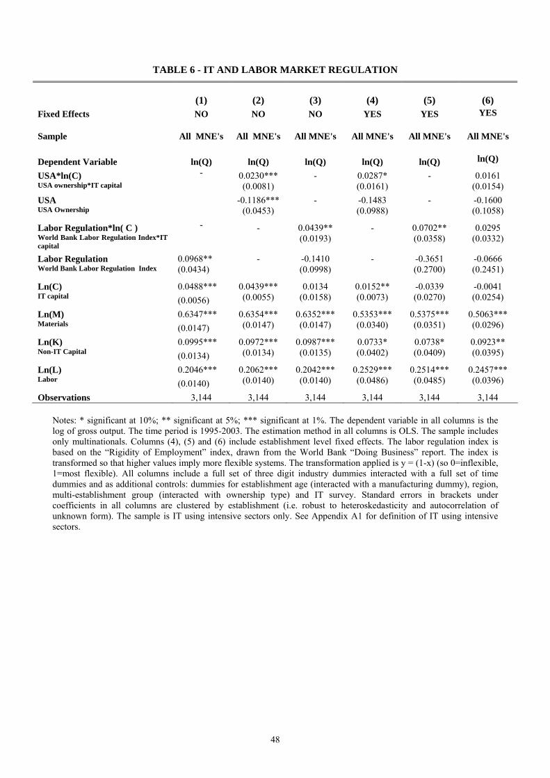
48

TABLE 6 - IT AND LABOR MARKET REGULATION

(1) (2) (3)

(4) (5) (6) Fixed Effects NO NO NO YES YES YES

Sample All MNE's All MNE's All MNE's All MNE's All MNE's All MNE's

Dependent Variable ln(Q) ln(Q) ln(Q) ln(Q) ln(Q) ln(Q)

USA*ln(C) - 0.0230*** - 0.0287* - 0.0161 USA ownership*IT capital (0.0081) (0.0161) (0.0154) USA -0.1186*** - -0.1483 - -0.1600 USA Ownership (0.0453) (0.0988) (0.1058)

Labor Regulation*ln( C ) - - 0.0439** - 0.0702** 0.0295 World Bank Labor Regulation Index*IT capital

(0.0193) (0.0358) (0.0332)

Labor Regulation 0.0968** - -0.1410 - -0.3651 -0.0666 World Bank Labor Regulation Index (0.0434) (0.0998) (0.2700) (0.2451)

Ln(C) 0.0488*** 0.0439*** 0.0134 0.0152** -0.0339 -0.0041 IT capital (0.0056) (0.0055) (0.0158) (0.0073) (0.0270) (0.0254)

Ln(M) 0.6347*** 0.6354*** 0.6352*** 0.5353*** 0.5375*** 0.5063*** Materials (0.0147) (0.0147) (0.0147) (0.0340) (0.0351) (0.0296)

Ln(K) 0.0995*** 0.0972*** 0.0987*** 0.0733* 0.0738* 0.0923** Non-IT Capital (0.0134) (0.0134) (0.0135) (0.0402) (0.0409) (0.0395)

Ln(L) 0.2046*** 0.2062*** 0.2042*** 0.2529*** 0.2514*** 0.2457*** Labor (0.0140) (0.0140) (0.0140) (0.0486) (0.0485) (0.0396)

Observations 3,144 3,144 3,144 3,144 3,144 3,144 Notes: * significant at 10%; ** significant at 5%; *** significant at 1%. The dependent variable in all columns is the log of gross output. The time period is 1995-2003. The estimation method in all columns is OLS. The sample includes only multinationals. Columns (4), (5) and (6) include establishment level fixed effects. The labor regulation index is based on the “Rigidity of Employment” index, drawn from the World Bank “Doing Business” report. The index is transformed so that higher values imply more flexible systems. The transformation applied is y = (1-x) (so 0=inflexible, 1=most flexible). All columns include a full set of three digit industry dummies interacted with a full set of time dummies and as additional controls: dummies for establishment age (interacted with a manufacturing dummy), region, multi-establishment group (interacted with ownership type) and IT survey. Standard errors in brackets under coefficients in all columns are clustered by establishment (i.e. robust to heteroskedasticity and autocorrelation of unknown form). The sample is IT using intensive sectors only. See Appendix A1 for definition of IT using intensive sectors.

49

TABLE A1 – BREAKDOWN OF THE INDUSTRIAL SECTORS BY IT USAGE

IT Intensive Sectors Manufacturing Services 18 Wearing apparel, dressing and dying of fur 51 Wholesale trades 22 Printing and publishing 52 Retail trade 29 Machinery and equipment 71 Renting of machinery and equipment 31 Manufacture of Electrical Machinery and Apparatus n.e.c. excludes 313 (insulated wire)

73 Research and development

33 Precision and optical instruments, excluding 331 (scientific instruments)

351 Building and repairing of ships and boats 353 Aircraft and spacecraft 352+359 Railroad equipment and transport equipment 36-37 miscellaneous manufacturing and recycling Other Sectors Manufacturing IT

producing sector?

Services IT producing sector?

15-16 Food drink and tobacco No 50 Sale, maintenance and repair of motor vehicles

No

17 Textiles No 55 Hotels and catering No 19 Leather and footwear No 60 Inland transport No 20 Wood No 61 Water transport No 21 Pulp and paper No 62 Air transport No 23 Mineral oil refining, coke and nuclear No 63 Supporting transport services, travel

agencies No

24 Chemicals No 64 Communications Yes 25 Rubber and plastics No 70 Real estate No 26 Non-metallic mineral products No 72 Computer services and related activity Yes 27 Basic metals No 741-743 Professional business services No 28 Fabricated metal products No 749 Other business activities n.e.c. No 30 Office machinery Yes 313 Insulated wire Yes Other sectors 321 Electronic valves and tubes Yes 10-14 Mining and quarrying No 322 Telecom equipment Yes 50-41 Utilities No 323 Radio and TV receivers Yes 45 Construction No 331 Scientific instruments Yes 34 Motor vehicles Notes: See text for definitions. IT intensive sectors are those that have above median IT capital flows as a proportion of total capital flows and are not IT producing sectors.

50

TABLE A2 - DESCRIPTIVE STATISTICS Panel A: All Establishments Variable Frequency Mean Median Standard

Deviation Employment 7,121 811.10 238.00 4,052.77 Gross Output 7,121 87,966.38 20,916.48 456,896.10 Value Added 7,121 29,787.61 7,052.00 167,798.70 IT Capital 7,121 1,030.60 77.44 10,820.69 ln(IT Capital) 7,121 4.46 4.35 2.03 Value Added per worker 7,121 40.43 29.53 55.19 Gross Output per worker 7,121 124.74 86.03 136.55 Materials per worker 7,121 82.38 47.23 103.52 Non-IT Capital per worker 7,121 85.28 48.56 112.54 IT Capital per worker 7,121 0.96 0.34 2.08 IT expenditure per worker 7,121 0.41 0.14 0.89 Material costs as a share of revenues 7,121 0.57 0.60 0.23 Employment costs as a share of revenues 7,121 0.83 0.64 0.86 Non-IT Capital as a share of revenues 7,121 0.30 0.26 0.20 IT Capital as a share of revenues 7,121 0.010 0.004 0.018 Age 7,121 8.38 5.00 6.74 Multigroup dummy (i.e. is establishment part of larger group?) 7,121 0.53 1.00 0.50

Panel B: Breakdown by Ownership Status and Sector

IT Capital over gross output (C/Q) Ln(IT Capital)

All

sectors

IT Using Intensive Sectors

Other Sectors

All sectors

IT Using Intensive Sectors

Other Sectors

All firms Mean 0.03 0.03 0.02 4.46 4.78 4.27 St. Deviation 0.04 0.04 0.04 2.03 2.06 1.99 Observations 7,121 2,703 4,418 7,121 2,703 4,418 US Multinationals Mean 0.04 0.04 0.03 5.57 5.69 5.46 St. Deviation 0.05 0.05 0.04 2.00 1.94 2.05 Observations 569 260 309 569 260 309 Other Multinationals Mean 0.03 0.03 0.03 5.18 5.34 5.07 St. Deviation 0.04 0.04 0.04 1.96 1.99 1.93 Observations 2,119 853 1,266 2,119 853 1,266 UK domestic Mean 0.02 0.03 0.02 3.98 4.33 3.79 St. Deviation 0.04 0.04 0.03 1.91 1.99 1.83 Observations 4,433 1,590 2,843 4,433 1,590 2,843

Notes: All monetary amounts are in sterling in year 2001 prices. Total stocks are constructed as described in the Appendix. All variables in units of 1,000s except ratios and employment.

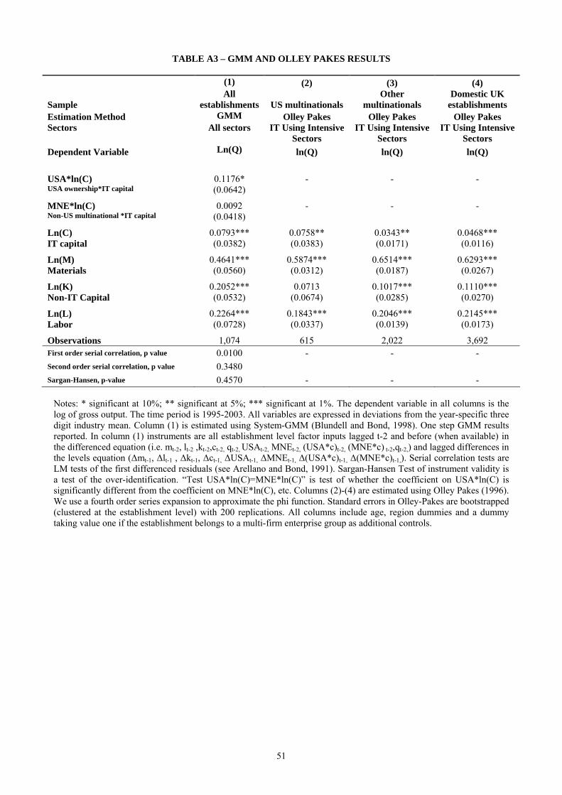
51

TABLE A3 – GMM AND OLLEY PAKES RESULTS

(1) (2) (3) (4)

Sample All

establishments US multinationals Other

multinationals Domestic UK

establishments Estimation Method GMM Olley Pakes Olley Pakes Olley Pakes Sectors All sectors IT Using Intensive

Sectors IT Using Intensive

Sectors IT Using Intensive

Sectors Dependent Variable Ln(Q) ln(Q) ln(Q) ln(Q) USA*ln(C) 0.1176* - - - USA ownership*IT capital (0.0642) MNE*ln(C) 0.0092 - - - Non-US multinational *IT capital (0.0418) Ln(C) 0.0793*** 0.0758** 0.0343** 0.0468*** IT capital (0.0382) (0.0383) (0.0171) (0.0116)

Ln(M) 0.4641*** 0.5874*** 0.6514*** 0.6293*** Materials (0.0560) (0.0312) (0.0187) (0.0267)

Ln(K) 0.2052*** 0.0713 0.1017*** 0.1110*** Non-IT Capital (0.0532) (0.0674) (0.0285) (0.0270)

Ln(L) 0.2264*** 0.1843*** 0.2046*** 0.2145*** Labor (0.0728) (0.0337) (0.0139) (0.0173)

Observations 1,074 615 2,022 3,692 First order serial correlation, p value 0.0100 - - - Second order serial correlation, p value 0.3480 Sargan-Hansen, p-value 0.4570 - - -

Notes: * significant at 10%; ** significant at 5%; *** significant at 1%. The dependent variable in all columns is the log of gross output. The time period is 1995-2003. All variables are expressed in deviations from the year-specific three digit industry mean. Column (1) is estimated using System-GMM (Blundell and Bond, 1998). One step GMM results reported. In column (1) instruments are all establishment level factor inputs lagged t-2 and before (when available) in the differenced equation (i.e. mt-2, lt-2 ,kt-2,ct-2, qt-2, USAt-2, MNEt-2, (USA*c)t-2, (MNE*c) t-2,qt-2,) and lagged differences in the levels equation (∆mt-1, ∆lt-1 , ∆kt-1, ∆ct-1, ∆USAt-1, ∆MNEt-1, ∆(USA*c)t-1, ∆(MNE*c)t-1,). Serial correlation tests are LM tests of the first differenced residuals (see Arellano and Bond, 1991). Sargan-Hansen Test of instrument validity is a test of the over-identification. “Test USA*ln(C)=MNE*ln(C)” is test of whether the coefficient on USA*ln(C) is significantly different from the coefficient on MNE*ln(C), etc. Columns (2)-(4) are estimated using Olley Pakes (1996). We use a fourth order series expansion to approximate the phi function. Standard errors in Olley-Pakes are bootstrapped (clustered at the establishment level) with 200 replications. All columns include age, region dummies and a dummy taking value one if the establishment belongs to a multi-firm enterprise group as additional controls.

52

TABLE A4 - NON RANDOM SELECTION OF US TAKEOVERS COMPARED TO OTHER TAKEOVERS?

(1) (2) (3) (4)

Dependent Variable = 1 if establishment taken over by US firm, = 0 for all other takeovers

US Takeover=1

US Takeover=1

US Takeover=1

US Takeover=1

Sample All takeovers

All takeovers

All except domestic takeovers

All except domestic takeovers

ln(C/L)t-1 0.0029 - -0.0003 -

(0.0095) (0.0365)

∆ln(C)t-1 - -0.0236 - -0.0876 (0.0246) (0.0714)

ln(L)t-1 0.0140 0.0108 -0.0183 -0.0222 (0.0106) (0.0111) (0.0377) (0.0379)

ln(K/L)t-1 0.0108 0.0109 -0.0174 -0.0346 (0.0209) (0.0204) (0.0645) (0.0650)

ln(Q/L)t-1 0.0236 0.0270 0.0333 0.0580 (0.0269) (0.0263) (0.0860) (0.0843)

Age -0.0014 -0.0017 -0.0003 -0.0014 (0.0038) (0.0039) (0.0085) (0.0087)

Observations 563 563 190 190 Notes: * significant at 10%; ** significant at 5%; *** significant at 1%. The dependent variable in all columns is a dummy taking value 1 if the establishment is taken over by a US Multinational and zero otherwise. Takeovers by UK firms (“domestics”) are excluded in columns (3)-(4). The time period is 1995-2003. All columns include two digit industry dummies, region and year dummies. The estimation method in all columns is by a linear probability model. Standard errors in brackets under coefficients are robust to heteroskedasticity.

Figure 1: Output per hour in Europe and the US, 1980-2005

2530

3540

4550

Out

put p

er h

our w

orke

d, 2

005

US

$

1980 1985 1990 1995 2000 2005year

US

Europe

Notes: Productivity measured by GDP per hour in 2005 US $ PPPs. The countries included in the “EU 15” group are: Austria, Belgium, Denmark, Finland, France, Germany, UK, Greece, Italy, Ireland, Luxembourg, Portugal, Spain, Sweden, and Netherlands. Labor productivity per hour worked in 2005 US$. Source: The Conference Board and Groningen Growth and Development Centre, Total Economy Database.

02

46

8IT

Cap

ital S

tock

per

Hou

rs W

orke

d, 2

000

US$

1980 1985 1990 1995 2000 2005year

IT Capital Stock per Hours WorkedFigure 2: IT capital per hour in Europe and the US, 1980-2005

Notes: IT capital stock (in unit dollars) per hour worked. IT capital stock measured using perpetual inventory method and common assumptions on hedonics and depreciation. 2005 US $ PPPs The countries included in the “EU 15” group are: Austria, Belgium, Denmark, Finland, France, Germany, UK, Greece, Italy, Ireland, Luxembourg, Portugal, Spain, Sweden and the Netherlands. Labour productivity per hour worked in 2005 US$ using PPPs. Source: Marcel P. Timmer, Gerard Ypma and Bart van Ark, “IT in the European Union: Driving Productivity Convergence?”, Research Memorandum GD-67, Groningen Growth and Development Centre, October 2003, Appendix Tables, updated June 2005.

US

Europe

Figure 2: IT capital per hour in Europe and the US, 1980-2005

European Firms 4.13

4.93US Firms

Domestic Firms, in Europe

4.87

3.67

4.11

Non-US Multinational subsidiaries, in Europe

US Multinational subsidiaries, in Europe

Figure 3a: Organizational devolvement,firms by country of location

Figure 3b: Organizational devolvement, firms by country of ownership

Notes: In Figures 3a and 3b the “Organizational devolvement” score is the average score for the 2 organizational questions for 548 firms in the US (219), UK (98) and France and Germany (231). The questions are taken exactly from Bresnahan et al. (2002) covering “Task allocation” and “Pace setting” where a higher scores indicate greater worker autonomy. Full survey details in Bloom and Van Reenen (2007). In Figure 3c the source is the WIRS data (1984 and 1990) which plots the proportion of establishments experiencing organizational change in previous 3 years (all establishments in the UK). US MNEs (N=190), Non-US MNEs (N=147), Domestic (N=2848). Senior manager is asked “whether there has been any change in work organization not involving new plant/equipment in the past three years”. In Figure 3d the source is the CIS data: we plot the proportion of establishments experiencing organizational or managerial change in previous 3 years. The firm is asked “Did your enterprise make major changes in the following areas of business structure and practices during the three year period 1998-2001?” with answers to either “Advanced Management techniques” or “Major changes in organizational structure” recorded as an organizational change.

0.56

0.66

0.77

Domestic Firms

Non-US Multinationals

US Multinationals

0.52

0.44

0.40Domestic Firms

Non-US Multinationals

US Multinationals

Figure 3c: Organizational change in the UK during 1981-1990

Figure 3d: Organizational change in the UK during 1998-2000

Figure 4: Decentralization (O) by US and European firms, model results

US

Europe

Notes: Results from the numerical simulation of the theoretical model 1980-2015 (the full simulation was run 1970-2025). See text for details. Decentralization is the value of O (between 0 for full centralization and 1 for full decentralization).

US

Europe

Figure 5: IT per unit of labor, log(C/L), in US and European firms, model results

Figure 6: Labor productivity, log(Q/L), in US and European firms, model results

US

Europe

Notes: Results from the numerical simulation of the theoretical model 1980-2015 (the full simulation was run 1970-2025). See text for details. Productivity is output per worker. Decentralization is the value of O (between 0 for full centralization and 1 for full decentralization).

US

Europe

Figure 7: Decentralization (O) by plants taken over by US multinationals: model results

US takeover of European plant

Figure 8: IT Intensity vs. Flexibility of Employment Index

Notes: The sample includes only establishments of multinationals in IT using sectors. Each point represents average IT intensity (IT capital divided by employment normalized by the three digit industry average) by country. Each country average is based on at least ten observations and three digit industries with fewer than 10 observations are excluded. The labour regulation index is the “Rigidity of Employment” index, drawn from the World Bank “Doing Business” report.

Australia (16)Australia (16)Australia (16)Australia (16)Australia (16)Australia (16)Australia (16)Australia (16)Australia (16)Australia (16)Australia (16)Australia (16)Australia (16)Australia (16)Australia (16)

Belgium (17)Belgium (17)Belgium (17)Belgium (17)Belgium (17)Belgium (17)Belgium (17)Belgium (17)Belgium (17)Belgium (17)Belgium (17)Belgium (17)Belgium (17)Belgium (17)Belgium (17)Belgium (17)Belgium (17)

Canada (27)Canada (27)Canada (27)Canada (27)Canada (27)Canada (27)Canada (27)Canada (27)Canada (27)Canada (27)Canada (27)Canada (27)Canada (27)Canada (27)Canada (27)Canada (27)Canada (27)Canada (27)Canada (27)Canada (27)Canada (27)Canada (27)Canada (27)Canada (27)Canada (27)Canada (27)Canada (27)Denmark (22)Denmark (22)Denmark (22)Denmark (22)Denmark (22)Denmark (22)Denmark (22)Denmark (22)Denmark (22)Denmark (22)Denmark (22)Denmark (22)Denmark (22)Denmark (22)Denmark (22)Denmark (22)Denmark (22)Denmark (22)Denmark (22)Denmark (22)Denmark (22)Denmark (22)

Finland (15)Finland (15)Finland (15)Finland (15)Finland (15)Finland (15)Finland (15)Finland (15)Finland (15)Finland (15)Finland (15)Finland (15)Finland (15)

France (202)France (202)France (202)France (202)France (202)France (202)France (202)France (202)France (202)France (202)France (202)France (202)France (202)France (202)France (202)France (202)France (202)France (202)France (202)France (202)France (202)France (202)France (202)France (202)France (202)France (202)France (202)France (202)France (202)France (202)France (202)France (202)France (202)France (202)France (202)France (202)France (202)France (202)France (202)France (202)France (202)France (202)France (202)France (202)France (202)France (202)France (202)France (202)France (202)France (202)France (202)France (202)France (202)France (202)France (202)France (202)France (202)France (202)France (202)France (202)France (202)France (202)France (202)France (202)France (202)France (202)France (202)France (202)France (202)France (202)France (202)France (202)France (202)France (202)France (202)France (202)France (202)France (202)France (202)France (202)France (202)France (202)France (202)France (202)France (202)France (202)France (202)France (202)France (202)France (202)France (202)France (202)France (202)France (202)France (202)France (202)France (202)France (202)France (202)France (202)France (202)France (202)France (202)France (202)France (202)France (202)France (202)France (202)France (202)France (202)France (202)France (202)France (202)France (202)France (202)France (202)France (202)France (202)France (202)France (202)France (202)France (202)France (202)France (202)France (202)France (202)France (202)France (202)France (202)France (202)France (202)France (202)France (202)France (202)France (202)France (202)France (202)France (202)France (202)France (202)France (202)France (202)France (202)France (202)France (202)France (202)France (202)France (202)France (202)France (202)France (202)France (202)France (202)France (202)France (202)France (202)France (202)France (202)France (202)France (202)France (202)France (202)France (202)France (202)France (202)France (202)France (202)France (202)France (202)France (202)France (202)France (202)France (202)France (202)France (202)France (202)France (202)France (202)France (202)France (202)France (202)France (202)France (202)France (202)France (202)France (202)France (202)France (202)France (202)France (202)France (202)France (202)France (202)France (202)France (202)France (202) Germany (254)Germany (254)Germany (254)Germany (254)Germany (254)Germany (254)Germany (254)Germany (254)Germany (254)Germany (254)Germany (254)Germany (254)Germany (254)Germany (254)Germany (254)Germany (254)Germany (254)Germany (254)Germany (254)Germany (254)Germany (254)Germany (254)Germany (254)Germany (254)Germany (254)Germany (254)Germany (254)Germany (254)Germany (254)Germany (254)Germany (254)Germany (254)Germany (254)Germany (254)Germany (254)Germany (254)Germany (254)Germany (254)Germany (254)Germany (254)Germany (254)Germany (254)Germany (254)Germany (254)Germany (254)Germany (254)Germany (254)Germany (254)Germany (254)Germany (254)Germany (254)Germany (254)Germany (254)Germany (254)Germany (254)Germany (254)Germany (254)Germany (254)Germany (254)Germany (254)Germany (254)Germany (254)Germany (254)Germany (254)Germany (254)Germany (254)Germany (254)Germany (254)Germany (254)Germany (254)Germany (254)Germany (254)Germany (254)Germany (254)Germany (254)Germany (254)Germany (254)Germany (254)Germany (254)Germany (254)Germany (254)Germany (254)Germany (254)Germany (254)Germany (254)Germany (254)Germany (254)Germany (254)Germany (254)Germany (254)Germany (254)Germany (254)Germany (254)Germany (254)Germany (254)Germany (254)Germany (254)Germany (254)Germany (254)Germany (254)Germany (254)Germany (254)Germany (254)Germany (254)Germany (254)Germany (254)Germany (254)Germany (254)Germany (254)Germany (254)Germany (254)Germany (254)Germany (254)Germany (254)Germany (254)Germany (254)Germany (254)Germany (254)Germany (254)Germany (254)Germany (254)Germany (254)Germany (254)Germany (254)Germany (254)Germany (254)Germany (254)Germany (254)Germany (254)Germany (254)Germany (254)Germany (254)Germany (254)Germany (254)Germany (254)Germany (254)Germany (254)Germany (254)Germany (254)Germany (254)Germany (254)Germany (254)Germany (254)Germany (254)Germany (254)Germany (254)Germany (254)Germany (254)Germany (254)Germany (254)Germany (254)Germany (254)Germany (254)Germany (254)Germany (254)Germany (254)Germany (254)Germany (254)Germany (254)Germany (254)Germany (254)Germany (254)Germany (254)Germany (254)Germany (254)Germany (254)Germany (254)Germany (254)Germany (254)Germany (254)Germany (254)Germany (254)Germany (254)Germany (254)Germany (254)Germany (254)Germany (254)Germany (254)Germany (254)Germany (254)Germany (254)Germany (254)Germany (254)Germany (254)Germany (254)Germany (254)Germany (254)Germany (254)Germany (254)Germany (254)Germany (254)Germany (254)Germany (254)Germany (254)Germany (254)Germany (254)Germany (254)Germany (254)Germany (254)Germany (254)Germany (254)Germany (254)Germany (254)Germany (254)Germany (254)Germany (254)Germany (254)Germany (254)Germany (254)Germany (254)Germany (254)Germany (254)Germany (254)Germany (254)Germany (254)Germany (254)Germany (254)Germany (254)Germany (254)Germany (254)Germany (254)Germany (254)Germany (254)Germany (254)Germany (254)Germany (254)Germany (254)Germany (254)Germany (254)Germany (254)Germany (254)Germany (254)Germany (254)Germany (254)Germany (254)Germany (254)Germany (254)Germany (254)Germany (254)Germany (254)Germany (254)Germany (254)Germany (254)Germany (254)Germany (254)Germany (254)Germany (254)

Japan (153)Japan (153)Japan (153)Japan (153)Japan (153)Japan (153)Japan (153)Japan (153)Japan (153)Japan (153)Japan (153)Japan (153)Japan (153)Japan (153)Japan (153)Japan (153)Japan (153)Japan (153)Japan (153)Japan (153)Japan (153)Japan (153)Japan (153)Japan (153)Japan (153)Japan (153)Japan (153)Japan (153)Japan (153)Japan (153)Japan (153)Japan (153)Japan (153)Japan (153)Japan (153)Japan (153)Japan (153)Japan (153)Japan (153)Japan (153)Japan (153)Japan (153)Japan (153)Japan (153)Japan (153)Japan (153)Japan (153)Japan (153)Japan (153)Japan (153)Japan (153)Japan (153)Japan (153)Japan (153)Japan (153)Japan (153)Japan (153)Japan (153)Japan (153)Japan (153)Japan (153)Japan (153)Japan (153)Japan (153)Japan (153)Japan (153)Japan (153)Japan (153)Japan (153)Japan (153)Japan (153)Japan (153)Japan (153)Japan (153)Japan (153)Japan (153)Japan (153)Japan (153)Japan (153)Japan (153)Japan (153)Japan (153)Japan (153)Japan (153)Japan (153)Japan (153)Japan (153)Japan (153)Japan (153)Japan (153)Japan (153)Japan (153)Japan (153)Japan (153)Japan (153)Japan (153)Japan (153)Japan (153)Japan (153)Japan (153)Japan (153)Japan (153)Japan (153)Japan (153)Japan (153)Japan (153)Japan (153)Japan (153)Japan (153)Japan (153)Japan (153)Japan (153)Japan (153)Japan (153)Japan (153)Japan (153)Japan (153)Japan (153)Japan (153)Japan (153)Japan (153)Japan (153)Japan (153)Japan (153)Japan (153)Japan (153)Japan (153)Japan (153)Japan (153)Japan (153)Japan (153)Japan (153)Japan (153)Japan (153)Japan (153)Japan (153)Japan (153)Japan (153)Japan (153)Japan (153)Japan (153)Japan (153)Japan (153)Japan (153)Japan (153)Japan (153)Japan (153)Japan (153)Japan (153)Japan (153)

Netherlands (218)Netherlands (218)Netherlands (218)Netherlands (218)Netherlands (218)Netherlands (218)Netherlands (218)Netherlands (218)Netherlands (218)Netherlands (218)Netherlands (218)Netherlands (218)Netherlands (218)Netherlands (218)Netherlands (218)Netherlands (218)Netherlands (218)Netherlands (218)Netherlands (218)Netherlands (218)Netherlands (218)Netherlands (218)Netherlands (218)Netherlands (218)Netherlands (218)Netherlands (218)Netherlands (218)Netherlands (218)Netherlands (218)Netherlands (218)Netherlands (218)Netherlands (218)Netherlands (218)Netherlands (218)Netherlands (218)Netherlands (218)Netherlands (218)Netherlands (218)Netherlands (218)Netherlands (218)Netherlands (218)Netherlands (218)Netherlands (218)Netherlands (218)Netherlands (218)Netherlands (218)Netherlands (218)Netherlands (218)Netherlands (218)Netherlands (218)Netherlands (218)Netherlands (218)Netherlands (218)Netherlands (218)Netherlands (218)Netherlands (218)Netherlands (218)Netherlands (218)Netherlands (218)Netherlands (218)Netherlands (218)Netherlands (218)Netherlands (218)Netherlands (218)Netherlands (218)Netherlands (218)Netherlands (218)Netherlands (218)Netherlands (218)Netherlands (218)Netherlands (218)Netherlands (218)Netherlands (218)Netherlands (218)Netherlands (218)Netherlands (218)Netherlands (218)Netherlands (218)Netherlands (218)Netherlands (218)Netherlands (218)Netherlands (218)Netherlands (218)Netherlands (218)Netherlands (218)Netherlands (218)Netherlands (218)Netherlands (218)Netherlands (218)Netherlands (218)Netherlands (218)Netherlands (218)Netherlands (218)Netherlands (218)Netherlands (218)Netherlands (218)Netherlands (218)Netherlands (218)Netherlands (218)Netherlands (218)Netherlands (218)Netherlands (218)Netherlands (218)Netherlands (218)Netherlands (218)Netherlands (218)Netherlands (218)Netherlands (218)Netherlands (218)Netherlands (218)Netherlands (218)Netherlands (218)Netherlands (218)Netherlands (218)Netherlands (218)Netherlands (218)Netherlands (218)Netherlands (218)Netherlands (218)Netherlands (218)Netherlands (218)Netherlands (218)Netherlands (218)Netherlands (218)Netherlands (218)Netherlands (218)Netherlands (218)Netherlands (218)Netherlands (218)Netherlands (218)Netherlands (218)Netherlands (218)Netherlands (218)Netherlands (218)Netherlands (218)Netherlands (218)Netherlands (218)Netherlands (218)Netherlands (218)Netherlands (218)Netherlands (218)Netherlands (218)Netherlands (218)Netherlands (218)Netherlands (218)Netherlands (218)Netherlands (218)Netherlands (218)Netherlands (218)Netherlands (218)Netherlands (218)Netherlands (218)Netherlands (218)Netherlands (218)Netherlands (218)Netherlands (218)Netherlands (218)Netherlands (218)Netherlands (218)Netherlands (218)Netherlands (218)Netherlands (218)Netherlands (218)Netherlands (218)Netherlands (218)Netherlands (218)Netherlands (218)Netherlands (218)Netherlands (218)Netherlands (218)Netherlands (218)Netherlands (218)Netherlands (218)Netherlands (218)Netherlands (218)Netherlands (218)Netherlands (218)Netherlands (218)Netherlands (218)Netherlands (218)Netherlands (218)Netherlands (218)Netherlands (218)Netherlands (218)Netherlands (218)Netherlands (218)Netherlands (218)Netherlands (218)Netherlands (218)Netherlands (218)Netherlands (218)Netherlands (218)Netherlands (218)Netherlands (218)Netherlands (218)Netherlands (218)Netherlands (218)Netherlands (218)Netherlands (218)Netherlands (218)Netherlands (218)Netherlands (218)Netherlands (218)Netherlands (218)Netherlands (218)Netherlands (218)Netherlands (218)Netherlands (218)Netherlands (218)Netherlands (218)Netherlands (218)Netherlands (218)Netherlands (218)Netherlands (218)Netherlands (218)Netherlands (218)Netherlands (218)Netherlands (218)

South Africa (12)South Africa (12)South Africa (12)South Africa (12)South Africa (12)South Africa (12)South Africa (12)South Africa (12)South Africa (12)South Africa (12)South Africa (12)South Africa (12)

Sweden (51)Sweden (51)Sweden (51)Sweden (51)Sweden (51)Sweden (51)Sweden (51)Sweden (51)Sweden (51)Sweden (51)Sweden (51)Sweden (51)Sweden (51)Sweden (51)Sweden (51)Sweden (51)Sweden (51)Sweden (51)Sweden (51)Sweden (51)Sweden (51)Sweden (51)Sweden (51)Sweden (51)Sweden (51)Sweden (51)Sweden (51)Sweden (51)Sweden (51)Sweden (51)Sweden (51)Sweden (51)Sweden (51)Sweden (51)Sweden (51)Sweden (51)Sweden (51)Sweden (51)Sweden (51)Sweden (51)Sweden (51)Sweden (51)Sweden (51)Sweden (51)Sweden (51)Sweden (51)Sweden (51)Sweden (51)

Switzerland (87)Switzerland (87)Switzerland (87)Switzerland (87)Switzerland (87)Switzerland (87)Switzerland (87)Switzerland (87)Switzerland (87)Switzerland (87)Switzerland (87)Switzerland (87)Switzerland (87)Switzerland (87)Switzerland (87)Switzerland (87)Switzerland (87)Switzerland (87)Switzerland (87)Switzerland (87)Switzerland (87)Switzerland (87)Switzerland (87)Switzerland (87)Switzerland (87)Switzerland (87)Switzerland (87)Switzerland (87)Switzerland (87)Switzerland (87)Switzerland (87)Switzerland (87)Switzerland (87)Switzerland (87)Switzerland (87)Switzerland (87)Switzerland (87)Switzerland (87)Switzerland (87)Switzerland (87)Switzerland (87)Switzerland (87)Switzerland (87)Switzerland (87)Switzerland (87)Switzerland (87)Switzerland (87)Switzerland (87)Switzerland (87)Switzerland (87)Switzerland (87)Switzerland (87)Switzerland (87)Switzerland (87)Switzerland (87)Switzerland (87)Switzerland (87)Switzerland (87)Switzerland (87)Switzerland (87)Switzerland (87)Switzerland (87)Switzerland (87)Switzerland (87)Switzerland (87)Switzerland (87)Switzerland (87)Switzerland (87)Switzerland (87)Switzerland (87)Switzerland (87)Switzerland (87)Switzerland (87)Switzerland (87)Switzerland (87)Switzerland (87)Switzerland (87)Switzerland (87)Switzerland (87)Switzerland (87)Switzerland (87)Switzerland (87)Switzerland (87)Switzerland (87)Switzerland (87)UK (1344)UK (1344)UK (1344)UK (1344)UK (1344)UK (1344)UK (1344)UK (1344)UK (1344)UK (1344)UK (1344)UK (1344)UK (1344)UK (1344)UK (1344)UK (1344)UK (1344)UK (1344)UK (1344)UK (1344)UK (1344)UK (1344)UK (1344)UK (1344)UK (1344)UK (1344)UK (1344)UK (1344)UK (1344)UK (1344)UK (1344)UK (1344)UK (1344)UK (1344)UK (1344)UK (1344)UK (1344)UK (1344)UK (1344)UK (1344)UK (1344)UK (1344)UK (1344)UK (1344)UK (1344)UK (1344)UK (1344)UK (1344)UK (1344)UK (1344)UK (1344)UK (1344)UK (1344)UK (1344)UK (1344)UK (1344)UK (1344)UK (1344)UK (1344)UK (1344)UK (1344)UK (1344)UK (1344)UK (1344)UK (1344)UK (1344)UK (1344)UK (1344)UK (1344)UK (1344)UK (1344)UK (1344)UK (1344)UK (1344)UK (1344)UK (1344)UK (1344)UK (1344)UK (1344)UK (1344)UK (1344)UK (1344)UK (1344)UK (1344)UK (1344)UK (1344)UK (1344)UK (1344)UK (1344)UK (1344)UK (1344)UK (1344)UK (1344)UK (1344)UK (1344)UK (1344)UK (1344)UK (1344)UK (1344)UK (1344)UK (1344)UK (1344)UK (1344)UK (1344)UK (1344)UK (1344)UK (1344)UK (1344)UK (1344)UK (1344)UK (1344)UK (1344)UK (1344)UK (1344)UK (1344)UK (1344)UK (1344)UK (1344)UK (1344)UK (1344)UK (1344)UK (1344)UK (1344)UK (1344)UK (1344)UK (1344)UK (1344)UK (1344)UK (1344)UK (1344)UK (1344)UK (1344)UK (1344)UK (1344)UK (1344)UK (1344)UK (1344)UK (1344)UK (1344)UK (1344)UK (1344)UK (1344)UK (1344)UK (1344)UK (1344)UK (1344)UK (1344)UK (1344)UK (1344)UK (1344)UK (1344)UK (1344)UK (1344)UK (1344)UK (1344)UK (1344)UK (1344)UK (1344)UK (1344)UK (1344)UK (1344)UK (1344)UK (1344)UK (1344)UK (1344)UK (1344)UK (1344)UK (1344)UK (1344)UK (1344)UK (1344)UK (1344)UK (1344)UK (1344)UK (1344)UK (1344)UK (1344)UK (1344)UK (1344)UK (1344)UK (1344)UK (1344)UK (1344)UK (1344)UK (1344)UK (1344)UK (1344)UK (1344)UK (1344)UK (1344)UK (1344)UK (1344)UK (1344)UK (1344)UK (1344)UK (1344)UK (1344)UK (1344)UK (1344)UK (1344)UK (1344)UK (1344)UK (1344)UK (1344)UK (1344)UK (1344)UK (1344)UK (1344)UK (1344)UK (1344)UK (1344)UK (1344)UK (1344)UK (1344)UK (1344)UK (1344)UK (1344)UK (1344)UK (1344)UK (1344)UK (1344)UK (1344)UK (1344)UK (1344)UK (1344)UK (1344)UK (1344)UK (1344)UK (1344)UK (1344)UK (1344)UK (1344)UK (1344)UK (1344)UK (1344)UK (1344)UK (1344)UK (1344)UK (1344)UK (1344)UK (1344)UK (1344)UK (1344)UK (1344)UK (1344)UK (1344)UK (1344)UK (1344)UK (1344)UK (1344)UK (1344)UK (1344)UK (1344)UK (1344)UK (1344)UK (1344)UK (1344)UK (1344)UK (1344)UK (1344)UK (1344)UK (1344)UK (1344)UK (1344)UK (1344)UK (1344)UK (1344)UK (1344)UK (1344)UK (1344)UK (1344)UK (1344)UK (1344)UK (1344)UK (1344)UK (1344)UK (1344)UK (1344)UK (1344)UK (1344)UK (1344)UK (1344)UK (1344)UK (1344)UK (1344)UK (1344)UK (1344)UK (1344)UK (1344)UK (1344)UK (1344)UK (1344)UK (1344)UK (1344)UK (1344)UK (1344)UK (1344)UK (1344)UK (1344)UK (1344)UK (1344)UK (1344)UK (1344)UK (1344)UK (1344)UK (1344)UK (1344)UK (1344)UK (1344)UK (1344)UK (1344)UK (1344)UK (1344)UK (1344)UK (1344)UK (1344)UK (1344)UK (1344)UK (1344)UK (1344)UK (1344)UK (1344)UK (1344)UK (1344)UK (1344)UK (1344)UK (1344)UK (1344)UK (1344)UK (1344)UK (1344)UK (1344)UK (1344)UK (1344)UK (1344)UK (1344)UK (1344)UK (1344)UK (1344)UK (1344)UK (1344)UK (1344)UK (1344)UK (1344)UK (1344)UK (1344)UK (1344)UK (1344)UK (1344)UK (1344)UK (1344)UK (1344)UK (1344)UK (1344)UK (1344)UK (1344)UK (1344)UK (1344)UK (1344)UK (1344)UK (1344)UK (1344)UK (1344)UK (1344)UK (1344)UK (1344)UK (1344)UK (1344)UK (1344)UK (1344)UK (1344)UK (1344)UK (1344)UK (1344)UK (1344)UK (1344)UK (1344)UK (1344)UK (1344)UK (1344)UK (1344)UK (1344)UK (1344)UK (1344)UK (1344)UK (1344)UK (1344)UK (1344)UK (1344)UK (1344)UK (1344)UK (1344)UK (1344)UK (1344)UK (1344)UK (1344)UK (1344)UK (1344)UK (1344)UK (1344)UK (1344)UK (1344)UK (1344)UK (1344)UK (1344)UK (1344)UK (1344)UK (1344)UK (1344)UK (1344)UK (1344)UK (1344)UK (1344)UK (1344)UK (1344)UK (1344)UK (1344)UK (1344)UK (1344)UK (1344)UK (1344)UK (1344)UK (1344)UK (1344)UK (1344)UK (1344)UK (1344)UK (1344)UK (1344)UK (1344)UK (1344)UK (1344)UK (1344)UK (1344)UK (1344)UK (1344)UK (1344)UK (1344)UK (1344)UK (1344)UK (1344)UK (1344)UK (1344)UK (1344)UK (1344)UK (1344)UK (1344)UK (1344)UK (1344)UK (1344)UK (1344)UK (1344)UK (1344)UK (1344)UK (1344)UK (1344)UK (1344)UK (1344)UK (1344)UK (1344)UK (1344)UK (1344)UK (1344)UK (1344)UK (1344)UK (1344)UK (1344)UK (1344)UK (1344)UK (1344)UK (1344)UK (1344)UK (1344)UK (1344)UK (1344)UK (1344)UK (1344)UK (1344)UK (1344)UK (1344)UK (1344)UK (1344)UK (1344)UK (1344)UK (1344)UK (1344)UK (1344)UK (1344)UK (1344)UK (1344)UK (1344)UK (1344)UK (1344)UK (1344)UK (1344)UK (1344)UK (1344)UK (1344)UK (1344)UK (1344)UK (1344)UK (1344)UK (1344)UK (1344)UK (1344)UK (1344)UK (1344)UK (1344)UK (1344)UK (1344)UK (1344)UK (1344)UK (1344)UK (1344)UK (1344)UK (1344)UK (1344)UK (1344)UK (1344)UK (1344)UK (1344)UK (1344)UK (1344)UK (1344)UK (1344)UK (1344)UK (1344)UK (1344)UK (1344)UK (1344)UK (1344)UK (1344)UK (1344)UK (1344)UK (1344)UK (1344)UK (1344)UK (1344)UK (1344)UK (1344)UK (1344)UK (1344)UK (1344)UK (1344)UK (1344)UK (1344)UK (1344)UK (1344)UK (1344)UK (1344)UK (1344)UK (1344)UK (1344)UK (1344)UK (1344)UK (1344)UK (1344)UK (1344)UK (1344)UK (1344)UK (1344)UK (1344)UK (1344)UK (1344)UK (1344)UK (1344)UK (1344)UK (1344)UK (1344)UK (1344)UK (1344)UK (1344)UK (1344)UK (1344)UK (1344)UK (1344)UK (1344)UK (1344)UK (1344)UK (1344)UK (1344)UK (1344)UK (1344)UK (1344)UK (1344)UK (1344)UK (1344)UK (1344)UK (1344)UK (1344)UK (1344)UK (1344)UK (1344)UK (1344)UK (1344)UK (1344)UK (1344)UK (1344)UK (1344)UK (1344)UK (1344)UK (1344)UK (1344)UK (1344)UK (1344)UK (1344)UK (1344)UK (1344)UK (1344)UK (1344)UK (1344)UK (1344)UK (1344)UK (1344)UK (1344)UK (1344)UK (1344)UK (1344)UK (1344)UK (1344)UK (1344)UK (1344)UK (1344)UK (1344)UK (1344)UK (1344)UK (1344)UK (1344)UK (1344)UK (1344)UK (1344)UK (1344)UK (1344)UK (1344)UK (1344)UK (1344)UK (1344)UK (1344)UK (1344)UK (1344)UK (1344)UK (1344)UK (1344)UK (1344)UK (1344)UK (1344)UK (1344)UK (1344)UK (1344)UK (1344)UK (1344)UK (1344)UK (1344)UK (1344)UK (1344)UK (1344)UK (1344)UK (1344)UK (1344)UK (1344)UK (1344)UK (1344)UK (1344)UK (1344)UK (1344)UK (1344)UK (1344)UK (1344)UK (1344)UK (1344)UK (1344)UK (1344)UK (1344)UK (1344)UK (1344)UK (1344)UK (1344)UK (1344)UK (1344)UK (1344)UK (1344)UK (1344)UK (1344)UK (1344)UK (1344)UK (1344)UK (1344)UK (1344)UK (1344)UK (1344)UK (1344)UK (1344)UK (1344)UK (1344)UK (1344)UK (1344)UK (1344)UK (1344)UK (1344)UK (1344)UK (1344)UK (1344)UK (1344)UK (1344)UK (1344)UK (1344)UK (1344)UK (1344)UK (1344)UK (1344)UK (1344)UK (1344)UK (1344)UK (1344)UK (1344)UK (1344)UK (1344)UK (1344)UK (1344)UK (1344)UK (1344)UK (1344)UK (1344)UK (1344)UK (1344)UK (1344)UK (1344)UK (1344)UK (1344)UK (1344)UK (1344)UK (1344)UK (1344)UK (1344)UK (1344)UK (1344)UK (1344)UK (1344)UK (1344)UK (1344)UK (1344)UK (1344)UK (1344)UK (1344)UK (1344)UK (1344)UK (1344)UK (1344)UK (1344)UK (1344)UK (1344)UK (1344)UK (1344)UK (1344)UK (1344)UK (1344)UK (1344)UK (1344)UK (1344)UK (1344)UK (1344)UK (1344)UK (1344)UK (1344)UK (1344)UK (1344)UK (1344)UK (1344)UK (1344)UK (1344)UK (1344)UK (1344)UK (1344)UK (1344)UK (1344)UK (1344)UK (1344)UK (1344)UK (1344)UK (1344)UK (1344)UK (1344)UK (1344)UK (1344)UK (1344)UK (1344)UK (1344)UK (1344)UK (1344)UK (1344)UK (1344)UK (1344)UK (1344)UK (1344)UK (1344)UK (1344)UK (1344)UK (1344)UK (1344)UK (1344)UK (1344)UK (1344)UK (1344)UK (1344)UK (1344)UK (1344)UK (1344)UK (1344)UK (1344)UK (1344)UK (1344)UK (1344)UK (1344)UK (1344)UK (1344)UK (1344)UK (1344)UK (1344)UK (1344)UK (1344)UK (1344)UK (1344)UK (1344)UK (1344)UK (1344)UK (1344)UK (1344)UK (1344)UK (1344)UK (1344)UK (1344)UK (1344)UK (1344)UK (1344)UK (1344)UK (1344)UK (1344)UK (1344)UK (1344)UK (1344)UK (1344)UK (1344)UK (1344)UK (1344)UK (1344)UK (1344)UK (1344)UK (1344)UK (1344)UK (1344)UK (1344)UK (1344)UK (1344)UK (1344)UK (1344)UK (1344)UK (1344)UK (1344)UK (1344)UK (1344)UK (1344)UK (1344)UK (1344)UK (1344)UK (1344)UK (1344)UK (1344)UK (1344)UK (1344)UK (1344)UK (1344)UK (1344)UK (1344)UK (1344)UK (1344)UK (1344)UK (1344)UK (1344)UK (1344)UK (1344)UK (1344)UK (1344)UK (1344)UK (1344)UK (1344)UK (1344)UK (1344)UK (1344)UK (1344)UK (1344)UK (1344)UK (1344)UK (1344)UK (1344)UK (1344)UK (1344)UK (1344)UK (1344)UK (1344)UK (1344)UK (1344)UK (1344)UK (1344)UK (1344)UK (1344)UK (1344)UK (1344)UK (1344)UK (1344)UK (1344)UK (1344)UK (1344)UK (1344)UK (1344)UK (1344)UK (1344)UK (1344)UK (1344)UK (1344)UK (1344)UK (1344)UK (1344)UK (1344)UK (1344)UK (1344)UK (1344)UK (1344)UK (1344)UK (1344)UK (1344)UK (1344)UK (1344)UK (1344)UK (1344)UK (1344)UK (1344)UK (1344)UK (1344)UK (1344)UK (1344)UK (1344)UK (1344)UK (1344)UK (1344)UK (1344)UK (1344)UK (1344)UK (1344)UK (1344)UK (1344)UK (1344)UK (1344)UK (1344)UK (1344)UK (1344)UK (1344)UK (1344)UK (1344)UK (1344)UK (1344)UK (1344)UK (1344)UK (1344)UK (1344)UK (1344)UK (1344)UK (1344)UK (1344)UK (1344)UK (1344)UK (1344)UK (1344)UK (1344)UK (1344)UK (1344)UK (1344)UK (1344)UK (1344)UK (1344)UK (1344)UK (1344)UK (1344)UK (1344)UK (1344)UK (1344)UK (1344)UK (1344)UK (1344)UK (1344)UK (1344)UK (1344)UK (1344)UK (1344)UK (1344)UK (1344)UK (1344)UK (1344)UK (1344)UK (1344)UK (1344)UK (1344)UK (1344)UK (1344)UK (1344)UK (1344)UK (1344)UK (1344)UK (1344)UK (1344)UK (1344)UK (1344)UK (1344)UK (1344)UK (1344)UK (1344)UK (1344)UK (1344)UK (1344)UK (1344)UK (1344)UK (1344)UK (1344)UK (1344)UK (1344)UK (1344)UK (1344)UK (1344)UK (1344)UK (1344)UK (1344)UK (1344)UK (1344)UK (1344)UK (1344)UK (1344)UK (1344)UK (1344)UK (1344)UK (1344)UK (1344)UK (1344)UK (1344)UK (1344)UK (1344)UK (1344)UK (1344)UK (1344)UK (1344)UK (1344)UK (1344)UK (1344)UK (1344)UK (1344)UK (1344)UK (1344)UK (1344)UK (1344)UK (1344)UK (1344)UK (1344)UK (1344)UK (1344)UK (1344)UK (1344)UK (1344)UK (1344)UK (1344)UK (1344)UK (1344)UK (1344)UK (1344)UK (1344)UK (1344)UK (1344)UK (1344)UK (1344)UK (1344)UK (1344)UK (1344)UK (1344)UK (1344)UK (1344)UK (1344)UK (1344)UK (1344)UK (1344)UK (1344)UK (1344)UK (1344)UK (1344)UK (1344)UK (1344)UK (1344)UK (1344)UK (1344)UK (1344)UK (1344)UK (1344)UK (1344)UK (1344)UK (1344)UK (1344)UK (1344)UK (1344)UK (1344)UK (1344)UK (1344)UK (1344)UK (1344)UK (1344)UK (1344)UK (1344)UK (1344)UK (1344)UK (1344)UK (1344)UK (1344)UK (1344)UK (1344)UK (1344)UK (1344)UK (1344)UK (1344)UK (1344)UK (1344)UK (1344)UK (1344)UK (1344)UK (1344)UK (1344)UK (1344)UK (1344)UK (1344)UK (1344)UK (1344)UK (1344)UK (1344)UK (1344)UK (1344)UK (1344)UK (1344)UK (1344)UK (1344)UK (1344)UK (1344)UK (1344)UK (1344)UK (1344)UK (1344)UK (1344)UK (1344)UK (1344)UK (1344)UK (1344)UK (1344)UK (1344)UK (1344)UK (1344)UK (1344)UK (1344)UK (1344)UK (1344)UK (1344)UK (1344)UK (1344)UK (1344)UK (1344)UK (1344)UK (1344)UK (1344)UK (1344)UK (1344)UK (1344)UK (1344)UK (1344)UK (1344)UK (1344)UK (1344)UK (1344)UK (1344)UK (1344)UK (1344)UK (1344)UK (1344)UK (1344)UK (1344)UK (1344)UK (1344)UK (1344)UK (1344)UK (1344)UK (1344)UK (1344)UK (1344)UK (1344)UK (1344)UK (1344)UK (1344)UK (1344)UK (1344)UK (1344)UK (1344)UK (1344)UK (1344)UK (1344)UK (1344)UK (1344)UK (1344)UK (1344)UK (1344)UK (1344)UK (1344)UK (1344)UK (1344)UK (1344)UK (1344)UK (1344)UK (1344)UK (1344)UK (1344)UK (1344)UK (1344)UK (1344)UK (1344)UK (1344)UK (1344)UK (1344)UK (1344)UK (1344)UK (1344)UK (1344)UK (1344)UK (1344)UK (1344)UK (1344)UK (1344)UK (1344)UK (1344)UK (1344)UK (1344)UK (1344)UK (1344)UK (1344)UK (1344)UK (1344)UK (1344)UK (1344)UK (1344)UK (1344)UK (1344)UK (1344)UK (1344)UK (1344)UK (1344)UK (1344)UK (1344)UK (1344)UK (1344)UK (1344)UK (1344)UK (1344)UK (1344)UK (1344)UK (1344)UK (1344)UK (1344)UK (1344)UK (1344)UK (1344)UK (1344)UK (1344)UK (1344)UK (1344)UK (1344)UK (1344)UK (1344)UK (1344)UK (1344)UK (1344)UK (1344)UK (1344)UK (1344)UK (1344)UK (1344)UK (1344)UK (1344)UK (1344)UK (1344)UK (1344)UK (1344)UK (1344)UK (1344)UK (1344)UK (1344)UK (1344)UK (1344)UK (1344)UK (1344)UK (1344)UK (1344)UK (1344)UK (1344)UK (1344)UK (1344)UK (1344)UK (1344)UK (1344)UK (1344)UK (1344)UK (1344)UK (1344)UK (1344)UK (1344)UK (1344)UK (1344)UK (1344)UK (1344)UK (1344)UK (1344)UK (1344)UK (1344)UK (1344)UK (1344)

USA (781)USA (781)USA (781)USA (781)USA (781)USA (781)USA (781)USA (781)USA (781)USA (781)USA (781)USA (781)USA (781)USA (781)USA (781)USA (781)USA (781)USA (781)USA (781)USA (781)USA (781)USA (781)USA (781)USA (781)USA (781)USA (781)USA (781)USA (781)USA (781)USA (781)USA (781)USA (781)USA (781)USA (781)USA (781)USA (781)USA (781)USA (781)USA (781)USA (781)USA (781)USA (781)USA (781)USA (781)USA (781)USA (781)USA (781)USA (781)USA (781)USA (781)USA (781)USA (781)USA (781)USA (781)USA (781)USA (781)USA (781)USA (781)USA (781)USA (781)USA (781)USA (781)USA (781)USA (781)USA (781)USA (781)USA (781)USA (781)USA (781)USA (781)USA (781)USA (781)USA (781)USA (781)USA (781)USA (781)USA (781)USA (781)USA (781)USA (781)USA (781)USA (781)USA (781)USA (781)USA (781)USA (781)USA (781)USA (781)USA (781)USA (781)USA (781)USA (781)USA (781)USA (781)USA (781)USA (781)USA (781)USA (781)USA (781)USA (781)USA (781)USA (781)USA (781)USA (781)USA (781)USA (781)USA (781)USA (781)USA (781)USA (781)USA (781)USA (781)USA (781)USA (781)USA (781)USA (781)USA (781)USA (781)USA (781)USA (781)USA (781)USA (781)USA (781)USA (781)USA (781)USA (781)USA (781)USA (781)USA (781)USA (781)USA (781)USA (781)USA (781)USA (781)USA (781)USA (781)USA (781)USA (781)USA (781)USA (781)USA (781)USA (781)USA (781)USA (781)USA (781)USA (781)USA (781)USA (781)USA (781)USA (781)USA (781)USA (781)USA (781)USA (781)USA (781)USA (781)USA (781)USA (781)USA (781)USA (781)USA (781)USA (781)USA (781)USA (781)USA (781)USA (781)USA (781)USA (781)USA (781)USA (781)USA (781)USA (781)USA (781)USA (781)USA (781)USA (781)USA (781)USA (781)USA (781)USA (781)USA (781)USA (781)USA (781)USA (781)USA (781)USA (781)USA (781)USA (781)USA (781)USA (781)USA (781)USA (781)USA (781)USA (781)USA (781)USA (781)USA (781)USA (781)USA (781)USA (781)USA (781)USA (781)USA (781)USA (781)USA (781)USA (781)USA (781)USA (781)USA (781)USA (781)USA (781)USA (781)USA (781)USA (781)USA (781)USA (781)USA (781)USA (781)USA (781)USA (781)USA (781)USA (781)USA (781)USA (781)USA (781)USA (781)USA (781)USA (781)USA (781)USA (781)USA (781)USA (781)USA (781)USA (781)USA (781)USA (781)USA (781)USA (781)USA (781)USA (781)USA (781)USA (781)USA (781)USA (781)USA (781)USA (781)USA (781)USA (781)USA (781)USA (781)USA (781)USA (781)USA (781)USA (781)USA (781)USA (781)USA (781)USA (781)USA (781)USA (781)USA (781)USA (781)USA (781)USA (781)USA (781)USA (781)USA (781)USA (781)USA (781)USA (781)USA (781)USA (781)USA (781)USA (781)USA (781)USA (781)USA (781)USA (781)USA (781)USA (781)USA (781)USA (781)USA (781)USA (781)USA (781)USA (781)USA (781)USA (781)USA (781)USA (781)USA (781)USA (781)USA (781)USA (781)USA (781)USA (781)USA (781)USA (781)USA (781)USA (781)USA (781)USA (781)USA (781)USA (781)USA (781)USA (781)USA (781)USA (781)USA (781)USA (781)USA (781)USA (781)USA (781)USA (781)USA (781)USA (781)USA (781)USA (781)USA (781)USA (781)USA (781)USA (781)USA (781)USA (781)USA (781)USA (781)USA (781)USA (781)USA (781)USA (781)USA (781)USA (781)USA (781)USA (781)USA (781)USA (781)USA (781)USA (781)USA (781)USA (781)USA (781)USA (781)USA (781)USA (781)USA (781)USA (781)USA (781)USA (781)USA (781)USA (781)USA (781)USA (781)USA (781)USA (781)USA (781)USA (781)USA (781)USA (781)USA (781)USA (781)USA (781)USA (781)USA (781)USA (781)USA (781)USA (781)USA (781)USA (781)USA (781)USA (781)USA (781)USA (781)USA (781)USA (781)USA (781)USA (781)USA (781)USA (781)USA (781)USA (781)USA (781)USA (781)USA (781)USA (781)USA (781)USA (781)USA (781)USA (781)USA (781)USA (781)USA (781)USA (781)USA (781)USA (781)USA (781)USA (781)USA (781)USA (781)USA (781)USA (781)USA (781)USA (781)USA (781)USA (781)USA (781)USA (781)USA (781)USA (781)USA (781)USA (781)USA (781)USA (781)USA (781)USA (781)USA (781)USA (781)USA (781)USA (781)USA (781)USA (781)USA (781)USA (781)USA (781)USA (781)USA (781)USA (781)USA (781)USA (781)USA (781)USA (781)USA (781)USA (781)USA (781)USA (781)USA (781)USA (781)USA (781)USA (781)USA (781)USA (781)USA (781)USA (781)USA (781)USA (781)USA (781)USA (781)USA (781)USA (781)USA (781)USA (781)USA (781)USA (781)USA (781)USA (781)USA (781)USA (781)USA (781)USA (781)USA (781)USA (781)USA (781)USA (781)USA (781)USA (781)USA (781)USA (781)USA (781)USA (781)USA (781)USA (781)USA (781)USA (781)USA (781)USA (781)USA (781)USA (781)USA (781)USA (781)USA (781)USA (781)USA (781)USA (781)USA (781)USA (781)USA (781)USA (781)USA (781)USA (781)USA (781)USA (781)USA (781)USA (781)USA (781)USA (781)USA (781)USA (781)USA (781)USA (781)USA (781)USA (781)USA (781)USA (781)USA (781)USA (781)USA (781)USA (781)USA (781)USA (781)USA (781)USA (781)USA (781)USA (781)USA (781)USA (781)USA (781)USA (781)USA (781)USA (781)USA (781)USA (781)USA (781)USA (781)USA (781)USA (781)USA (781)USA (781)USA (781)USA (781)USA (781)USA (781)USA (781)USA (781)USA (781)USA (781)USA (781)USA (781)USA (781)USA (781)USA (781)USA (781)USA (781)USA (781)USA (781)USA (781)USA (781)USA (781)USA (781)USA (781)USA (781)USA (781)USA (781)USA (781)USA (781)USA (781)USA (781)USA (781)USA (781)USA (781)USA (781)USA (781)USA (781)USA (781)USA (781)USA (781)USA (781)USA (781)USA (781)USA (781)USA (781)USA (781)USA (781)USA (781)USA (781)USA (781)USA (781)USA (781)USA (781)USA (781)USA (781)USA (781)USA (781)USA (781)USA (781)USA (781)USA (781)USA (781)USA (781)USA (781)USA (781)USA (781)USA (781)USA (781)USA (781)USA (781)USA (781)USA (781)USA (781)USA (781)USA (781)USA (781)USA (781)USA (781)USA (781)USA (781)USA (781)USA (781)USA (781)USA (781)USA (781)USA (781)USA (781)USA (781)USA (781)USA (781)USA (781)USA (781)USA (781)USA (781)USA (781)USA (781)USA (781)USA (781)USA (781)USA (781)USA (781)USA (781)USA (781)USA (781)USA (781)USA (781)USA (781)USA (781)USA (781)USA (781)USA (781)USA (781)USA (781)USA (781)USA (781)USA (781)USA (781)USA (781)USA (781)USA (781)USA (781)USA (781)USA (781)USA (781)USA (781)USA (781)USA (781)USA (781)USA (781)USA (781)USA (781)USA (781)USA (781)USA (781)USA (781)USA (781)USA (781)USA (781)USA (781)USA (781)USA (781)USA (781)USA (781)USA (781)USA (781)USA (781)USA (781)USA (781)USA (781)USA (781)USA (781)USA (781)USA (781)USA (781)USA (781)USA (781)USA (781)USA (781)USA (781)USA (781)USA (781)USA (781)USA (781)USA (781)USA (781)USA (781)USA (781)USA (781)USA (781)USA (781)USA (781)USA (781)USA (781)USA (781)USA (781)USA (781)USA (781)USA (781)USA (781)USA (781)USA (781)USA (781)USA (781)USA (781)USA (781)USA (781)USA (781)USA (781)USA (781)USA (781)USA (781)USA (781)USA (781)USA (781)USA (781)USA (781)USA (781)USA (781)USA (781)USA (781)USA (781)USA (781)USA (781)USA (781)USA (781)USA (781)USA (781)USA (781)USA (781)USA (781)USA (781)USA (781)USA (781)USA (781)USA (781)USA (781)USA (781)USA (781)USA (781)USA (781)USA (781)USA (781)USA (781)USA (781)USA (781)USA (781)USA (781)USA (781)USA (781)USA (781)USA (781)USA (781)USA (781)USA (781)USA (781)USA (781)USA (781)USA (781)USA (781)USA (781)

0.5

11.

5IT

cap

ital p

er e

mpl

oyee

rela

tive

to in

dust

ry a

vera

ge

.4 .6 .8 1World Bank Flexibility of Employment Index

(0=Most Strict Labour Regulations; 1=Most Flexible Labour Regulations)

1

0

US Europe

Year

Figure B1: Organizational change over time in the US and EU

c.1985 c.2006 c.2012 c.2020+

1 2 3 4 5Regime:

ORG

Wedge: US=Europe US>Europe US<Europe??

Notes: This figure illustrates the theoretical predictions of the model when we allow for adjustment costs in IT (see Appendix B for details). Note that these are analytic results rather than numerically simulated so the years are approximate. The “wedge” is the difference between actual and measured TFP (see equation (B2)). Regime 1 is where neither the EU nor US have begun adjusting organization (so O = 0). Regime 5 is where both the EU and US have fully adjusted their organization (so O = 1). In Regime 2 the US has started adjusting, but the EU has not, in Regime 3 both regions are adjusting and in Region 4 the US has fully adjusted and the EU is still adjusting.

CENTRE FOR ECONOMIC PERFORMANCE Recent Discussion Papers

787 Elizabeth O. Ananat Guy Michaels

The Effect of Marital Breakup on the Income Distribution of Women with Children

786 Willem H. Buiter Seigniorage

785 Gustavo Crespi Chiara Criscuolo Jonathan E. Haskel Matthew Slaughter

Productivity Growth, Knowledge Flows and Spillovers

784 Richard Layard Guy Mayraz Stephen Nickell

The Marginal Utility of Income

783 Gustavo Crespi Chiara Criscuolo Jonathan E. Haskel

Information Technology, Organisational Change and Productivity Growth: Evidence from UK Firms

782 Paul Castillo Carlos Montoro Vicente Tuesta

Inflation Premium and Oil Price Volatility

781 David Metcalf Why Has the British National Minimum Wage Had Little or No Impact on Employment?

780 Carlos Montoro Monetary Policy Committees and Interest Rate Smoothing

779 Sharon Belenzon Mark Schankerman

Harnessing Success: Determinants of University Technology Licensing Performance

778 Henry G. Overman Diego Puga Matthew A. Turner

Decomposing the Growth in Residential Land in the United States

777 Florence Kondylis Conflict-Induced Displacement and Labour Market Outcomes: Evidence from Post-War Bosnia and Herzegovina

776 Willem H. Buiter Is Numérairology the Future of Monetary Economics? Unbundling numéraire and medium of exchange through a virtual currency and a shadow exchange rate

775 Francesco Caselli Nicola Gennaioli

Economics and Politics of Alternative Institutional Reforms

774 Paul Willman Alex Bryson

Union Organization in Great Britain Prepared for symposium for the Journal of Labor Research on “The State of Unions: A Global Perspective”

773 Alan Manning The Plant Size-Effect: Agglomeration and Monopsony in Labour Markets

772 Guy Michaels The Effect of Trade on the Demand for Skill – Evidence from the Interstate Highway System

771 Gianluca Benigno Christoph Thoenissen

Consumption and Real Exchange Rates with Incomplete Markets and Non-Traded Goods

770 Michael Smart Daniel M. Sturm

Term Limits and Electoral Accountability

769 Andrew B. Bernard Stephen J. Redding Peter K. Schott

Multi-Product Firms and Trade Liberalization

768 Paul Willman Alex Bryson

Accounting for Collective Action: Resource Acquisition and Mobilization in British Unions

767 Anthony J. Venables Shifts in Economic Geography and their Causes

766 Guy Michaels The Long-Term Consequences of Regional Specialization

765 Fabrice Murtin American Economic Development Since the Civil War or the Virtue of Education

764 Carlo Rosa Giovanni Verga

The Impact of Central Bank Announcements on Asset Prices in Real Time: Testing the Efficiency of the Euribor Futures Market

763 Benjamin Aleman-Castilla

The Effect of Trade Liberalization on Informality and Wages: Evidence from Mexico

762 L. Rachel Ngai Roberto M. Samaniego

An R&D-Based Model of Multi-Sector Growth

761 Mariano Bosch Job Creation and Job Destruction in the Presence of Informal Labour Markets

760 Christian Hilber Frédéric Robert-Nicoud

Owners of Developed Land Versus Owners of Undeveloped Land: Why Land Use is More Constrained in the Bay Area than in Pittsburgh

759 William Nickell The CEP-OECD Institutions Data Set (1060-2004)

The Centre for Economic Performance Publications Unit Tel 020 7955 7673 Fax 020 7955 7595 Email info@cep.lse.ac.uk

Web site http://cep.lse.ac.uk