Ceramic silver impregnated pot filters for household drinking water treatment in developing countries Master of Science Thesis in Civil Engineering Sanitary Engineering Section Department of Water Management Faculty of Civil Engineering Delft University of Technology Doris van Halem November 2006 Committee: Prof. ir. J.C. van Dijk Delft University of Technology Sanitary Engineering Section Dr. ir. S.G.J. Heijman Delft University of Technology Sanitary Engineering Section Dr. ir. M.R. de Rooij Delft University of Technology Microlab Prof. dr. G.L. Amy UNESCO-IHE Institute for Water Education Water Engineering Department
Transcript
Ceramic silver impregnated pot filters for household drinking water treatment in developing countries
Master of Science Thesis in Civil Engineering
Sanitary Engineering Section
Department of Water Management
Faculty of Civil Engineering
Delft University of Technology
Doris van Halem
November 2006
Committee:
Prof. ir. J.C. van Dijk Delft University of Technology
Sanitary Engineering Section
Dr. ir. S.G.J. Heijman Delft University of Technology
Sanitary Engineering Section
Dr. ir. M.R. de Rooij Delft University of Technology
Microlab
Prof. dr. G.L. Amy UNESCO-IHE Institute for Water Education
Water Engineering Department
This study is executed in cooperation with the partners of the CSF project:
Aqua for All
Postbus 1072
3430 BB Nieuwegein
www.aquaforall.nl
Practica Foundation
Maerten Trompstraat 31
2628 RC Delft
www.practicafoundation.nl
Het Waterlaboratorium
J.W. Lucasweg 2
2031 BE Haarlem
www.hetwaterlaboratorium.nl
Kiwa Water Research
Groningerhaven 7
3433 PE Nieuwegein
www.kiwa.nl
Waterlaboratorium Noord
Rijksstraatweg 85
9756 AD Glimmen
www.wln.nl
- i -
Acknowledgements
This report is the result of the Master Thesis project of the Sanitary Engineering Section at the Faculty of Civil Engineering and Geosciences at Delft University of Technology. The subject of this project is the use of ceramic silver impregnated pot filters (CSF) for household drinking water treatment in developing countries.
I would like to thank all people involved in this research project, especially the members of my graduation committee. Hans van Dijk gave me the opportunity to execute this special project for my graduation and advised me on several occasions on both the complete story of my thesis and the fundamentals of my research. Bas Heijman was my supervisor and available for all my questions. Especially his knowledge on the techniques of research on membrane (nano)filtration was very useful in this study. Mario de Rooij of Microlab assisted and advised me on the use of mercury intrusion porosimetry and the elaboration of these data. I would like to thank Gary Amy for his involvement in this project with his international background at UNESCO-IHE.
This CSF research project is an initiative of Practica Foundation and Aqua for All Foundation. A group of experts from the Dutch drinking water sector have the responsible of an organisational and advising role. Special thanks go to Guus Soppe, Hans van der Jagt, Jan Kroesbergen, Eric Oude Vrielink and Henk Holtslag.
This project is done in cooperation with Dutch drinking water laboratories: Het Waterlaboratorium, Kiwa Water Research and Waterlaboratorium Noord. I would like to thank all employees involved in the analysis of the numerous samples. Furthermore I would like to thank Marcel Tielemans, Hilde Prummel and Robin Pistorius for their enthusiasm and involvement in this project.
Most of my work is done in the laboratory of Sanitary Engineering and I would like to thank Tonny Schuit for his assistance. Lesley Robertson of the laboratory of Microbiology gave me practical advice on the use of ‘bugs’ in the laboratory, thank you.
Last but not least, I would like to show much gratitude to my parents who have supported me throughout my education.
- ii -
- iii -
Executive Summary
Introduction
The World Health Organization (WHO)/UNICEF assessed in 2000 that 1.1 billion people do not have access to ‘improved drinking-water sources’. Interventions in hygiene, sanitation and water supply make proven contributors to controlling this disease burden. The ambitious target established in the ‘Millennium Development Goal1’ (MDG # 7) is “halving the proportion of people without sustainable access to safe water and basic sanitation by 2015”. Providing more than half a billion people with safe drinking water is a major task, especially because most of them are living in rural areas. Despite major efforts to deliver safe, piped, community water to the world’s population, the reality is that water supplies delivering safe water will not be available to these people on such a short term. According to the WHO a short-term solution to meet the basic need of safe drinking water can be found in household water treatment and safe storage (HWTS).
Ceramic silver impregnated pot filters (CSF) is a HWTS system developed by the Non-Governmental Organisation named Potters for Peace. After installing a production facility in Nicaragua, Potters for Peace has begun to scale up the filter production in other countries. This is done by involving local entrepreneurs to start their own CSF factories. Furthermore CSF is implemented by emergency relief organisations including the International Red Cross and Doctors without Borders. CSF is manufactured with local materials and skills and is therefore an inexpensive product ranging from US$5 to US$12. A mixture of clay, sawdust and water is pressed into a pot shape with press moulds. Once the filter element has its shape it is fired in an oven and impregnated with a layer of colloidal silver. Potters for Peace aims for the filter element to have a maximum pore size of 1 μm [PFP, 2001].
Since the introduction of the ceramic pot filters many reports have been published on the performance of these filters. The focus of these investigations has been the performance of CSF in the field and the improvement of the product and the manufacturing process. Brown and Sobsey [2006] observed an estimated 46% reduction in diarrhoea in filter users versus non filter users in a follow-up assessment in Cambodia. In the laboratory in Nicaragua, log10 reduction values2 between 1.8 and 4.9 of E.coli3 are reported [Lantagne, 2001], but the
1 The Millennium Development Goals are a blueprint agreed to by the member states of the United Nations and the world’s leading development institutions, September 2000. 2 Log10 reduction values are computed as the log10(influent/effluent); 1 LRV=90% reduction, 2 LRV=99% reduction, 3 LRV=99.9% reduction, and so on
Master Thesis: Ceramic Silver Impregnated Pot Filters
- iv -
measurements of these laboratory investigations are not numerous enough to be statistically reliable. In literature there is a lack of research on the application of colloidal silver on CSF. It is unknown if the contact time and surface area is sufficient to enhance microbial inactivation.
Objective
The objective of this study is to provide reliable performance data under laboratory conditions for ceramic silver impregnated pot filters to help speeding-up and scaling-up their implementation by organisations worldwide. This overall objective has been specified in sub-objectives to provide a base for the research approach: (i) determining the level of removal efficiency of pathogenic micro organisms by CSF; (ii) determining the occurrence of leaching and/or removal of metals; (iii) providing knowledge on the physical filter characteristics such as pore size distribution; (iv) investigating the effect and role of colloidal silver in CSF; (v) designing a test protocol to control the filter quality in the factories. This study is the first phase to acquire a ‘Declaration of Performance’ of the Dutch drinking water laboratories
Research approach
To provide reliable performance data the removal efficiency of 24 filters is monitored during a long-term study of 12 weeks in the laboratory of Sanitary Engineering. Ceramic silver impregnated pot filters are imported from 3 production locations; Cambodia, Ghana and Nicaragua. From Nicaragua also filters without the application of silver are imported. These filters are daily loaded with canal water to simulate the demand of a small family. The influent and effluent of the filters are measured weekly for: (i) pH, temperature and conductivity; (ii) turbidity; (iii) total coliforms and E.coli; (iv) relevant metals.
The situation of highly contaminated waters in rural areas of developing countries is translated to the laboratory by dosing high concentrations of indicator organisms:
i. Sulphite reducing Clostridium spores as an indicator for oocysts4 of protozoa;
ii. E.coli K12 as an indicator for pathogenic bacteria;
iii. MS2 bacteriophages as an indicator for viruses.
The demands and wishes of the consumers are considered during this study by monitoring the operation, cleaning procedure and the flavour and colour of the effluent water.
The microstructure of the filter material is of interest to completely understand the mechanisms of filtration in CSF. With mercury intrusion porosimetry, the direct method, bubble-point test and analytical model the following physical filter characteristics are determined: porosity, pore size distribution, total pore area, permeability, tortuosity, effective pore size, and filter discharge.
Conclusions and recommendations
The major findings from the long-term study are: (i) in 93% of the 144 taken 300mL samples no total coliforms were detected; (ii) log10 reduction values between 4 and 7 were reached for spikes with E.coli; (iii) sulphite reducing Clostridium spores (103-105 n/100mL) are successfully removed by all filters, with and without colloidal silver; (iv) MS2 bacteriophages are partially removed by CSF (LRV 0.5-3.0).
The effective pore size diameters measured with the bubble-point test have a mean of 40 μm. The data collected with mercury intrusion porosimetry show characteristic pore lengths in the filter material between 16 and 25 μm. It is obvious that these measured pores are much
3 Escherichia coli, a member of the coliform group, are almost exclusively of faecal origin and their presence confirms faecal contamination 4 Protozoa form protective stages, known as oocysts, which allow them to survive for long periods in water
Executive Summary
- v -
larger than the maximum of 1 μm pores aimed at by Potters for Peace. However, the effect of these pores on the removal efficiency is not great, since micro organisms much smaller than these pores are retained. It can therefore be concluded that the indicator organisms are removed by other mechanisms than absolute screening, namely mechanism of sedimentation, diffusion, inertia, turbulence and adsorption.
Filters manufactured in Nicaragua without the application of colloidal silver removed equally successful coliforms from the canal water as the filters with colloidal silver. Furthermore, for the retention of Clostridium spores colloidal silver proved not to be a necessity. High concentrations of E.coli are better removed by filters with silver, but still the achieved log removal is satisfactory for both filter types. Nevertheless, based on the results from this study can be concluded that the application of colloidal silver on CSF has a positive effect on the removal of E.coli K12. This is in contrast with MS2 bacteriophages, because these are surprisingly better retained by filters without the application of silver; this is most likely due to the reduced adsorptive pore (surface) area after coating with silver.
Metallic compounds are released from the filter material during filtration. Of all measured metallic compounds, especially the concentrations of arsenic in the effluent water are worrying. In the first week the mean concentration of the Cambodian filter reached almost 200 μg/L, and even after 12 weeks of usage the concentration was still slightly above the 10 μg /L WHO guideline with a mean of 17 μg /L. Silver leaches from the filter element also, visibly reducing the bacterial growth in the receptacle. But the concentrations of silver in the effluent water are insufficient to cause the cosmetic skin condition of argyria [WHO, 2006].
The main deficiency of CSF is the low filter discharge; during the 12-week long-term study all discharges reduce below 0.5 L/h. It must be taken into account that the reduction in flux depends on the raw water quality. Scrubbing of the filter elements has a temporarily effect on the discharge only. The measured fluxes are unacceptable; it is a basic requirement that CSF provides sufficient reliable water for a family. It is recommended that future research is done on the possibilities to increase the discharge. Furthermore the focus of the product improvement should be the increase of discharge without losing effectiveness of the removal of pathogenic micro organisms.
In this study filters were imported without specified information on the exact manufacturing method. Additionally, the filters did not origin from the same batch and are therefore probably not produced under the same conditions. These unknown variables have made it impossible to determine the replicability of CSF in this study and thus come to a ‘Declaration of Performance’ by the Dutch drinking water laboratories. Future research is therefore recommended after standardisation and documentation at the production locations. Especially the solid specification of the exact manufacturing method; type of clay, size of sawdust, moisture and heating etc are of importance.
It is recommended that future research is done on the effect of the application of colloidal silver: (i) at the production location to compare filters from the same batch with and without colloidal silver; (ii) the effect of silver on the adsorptive properties of the filter material in relation the adsorption of bacteriophages; (iii) the discussion on the need of colloidal silver in CSF, for it to be a safe household water treatment system.
The final recommendation of this study is that in case arsenic is known to be present in a region, the selected clay for the filter material is tested for the leaching of arsenic, before choosing it as the main substance of CSF.
Master Thesis: Ceramic Silver Impregnated Pot Filters
6 ANALYSIS OF THE RESULTS............................................................................. 63 6.1 MECHANISMS OF FILTRATION IN CSF ........................................................................ 63 6.2 REDUCTION IN FILTER DISCHARGE ............................................................................ 65 6.3 ROLE OF COLLOIDAL SILVER IN CSF .......................................................................... 67 6.4 FILTER QUALITY CONTROL ...................................................................................... 70
BIBLIOGRAPHY ...................................................................................................... 79 LIST OF FIGURES.................................................................................................... 83 LIST OF TABLES...................................................................................................... 85 APPENDICES........................................................................................................... 87
- 1 -
1 Introduction
Access to safe drinking water is essential to a person’s health, a basic human right and a component of effective policy for health protection [WHO, 2006]. In this context many organisations have initiated the development of drinking water treatment systems suitable for the tropical conditions in developing countries. Ceramic silver impregnated pot filters (CSF) is such a system developed by the non-governmental organisation ‘Potters for Peace’ and currently manufactured in many countries worldwide. The performance of CSF as a drinking water treatment system is the subject of this Master’s Thesis.
In the first section (1.1) of this chapter an introduction is given into ceramic silver impregnated pot filters. Section 1.2 overviews the literature on previous research regarding CSF and silver. The problem description and objective of this Master’s Thesis are outlined in section 1.3 and 1.4. Section 1.5 gives an overview of the restrictions of this study; constraints, guidelines and assumptions. In section 1.6 the research approach is presented, including the collection of performance data and experiments performed to determine the porosity of the filter material. In the final section (1.7) the contents of this report is outlined.
1.1 Ceramic silver impregnated pot filter (CSF)
The need for household water treatment systems in developing countries has lead to the introduction of ceramic silver impregnated pot filters. One of the advantages of CSF is that it is produced with local materials and skills, as described in this section.
1.1.1 Household water treatment
The World Health Organization (WHO)/UNICEF assessed in 2000 that 1.1 billion people do not have access to ‘improved drinking-water sources’. Consumption of unsafe water continues to be one of the major causes of the 2.2 million diarrhoeal disease deaths occurring annually, mostly children in developing countries [Sobsey, 2002]. Interventions in hygiene, sanitation and water supply make proven contributors to controlling this disease burden. The ambitious target established in the ‘Millennium Development Goal5’ (MDG # 7) is “halving the proportion of people without sustainable access to safe water and basic sanitation by 2015”.
5 The Millennium Development Goals are a blueprint agreed to by the member states of the United Nations and the world’s leading development institutions, September 2000.
Master Thesis: Ceramic Silver Impregnated Pot Filters
- 2 -
Providing more than half a billion people with safe drinking water is a major task, especially since most of them are living in rural areas. Despite major efforts to deliver safe, piped, community water to the world’s population, the reality is that water supplies delivering safe water will not be available to these people in such a short term. It is not an option to wait for the long-term solution of microbiologically reliable drinking water through distribution systems. According to WHO a short-term solution to meet the basic need of safe drinking water can be found in household water treatment and safe storage (HWTS). Apart from the advantage of a relatively rapid implementation of HWTS, recontamination can be prevented by treating the water at home. Recontamination occurs between point of delivery and consumption, both during transport and in the homes. During the past decades several point-of-use treatment systems (Figure 1.1) have been developed and are in use all over the world.
An appropriate technology complies with WHO guidelines on the quality and quantity of water. It ensures the guarantee that water for personal or domestic use is safe and therefore free from micro organisms, chemical substances and hazards that constitute a threat to a person's health.
Potters for Peace (PFP) “seeks to build an independent, non-profit, international network of potters concerned with peace and justice issues. We will maintain this concern principally through interchanges involving potters of the (overdeveloped) North and (underdeveloped) South. PFP aims to provide socially responsible assistance to pottery groups and individuals in their search for stability and improvement of ceramic production, and in the preservation of their cultural inheritance” [PFP, 2001]. In this context PFP started to introduce ceramic colloidal silver-impregnated pot filters (CSF) in developing countries.
After installing a production facility in Nicaragua, Potters for Peace has begun to scale up the filter production in other countries. This is done by involving local entrepreneurs to start their own factories. In the year 2000, factories were established in Mexico, Bangladesh and Cambodia, followed by factories in Haiti, Guatemala, El Salvador, Nepal, Pakistan, Uzbekistan and Ghana in 2001 and 2002. Furthermore CSF are implemented by emergency relief organisations including the International Red Cross and Doctors without Borders.
Chapter 1: Introduction
- 3 -
1.1.3 Manufacturing CSF
The following section is roughly based on the brochure of IDEASS Nicaragua ‘FILTRÓN, Ceramic filter for drinking water’. The manufacturing process of CSF begins by grinding dry clay in a hammer mill and sieving it through a screen mesh (2 mm). Sieved sawdust (3 mm) is added to the clay and mixed either by hand or in a mixer. Then, water is slowly added to the mixture followed by another mixture period to obtain a homogenous consistency. The clay/sawdust/water mixture is pressed into shape by a hydraulic press with purpose-built moulds (appendix I.1). Now the shape of the filter is obtained and the filter is marked with a unique code. Before the filters can be fired in an oven the filters have to dry for 4 to 21 days, depending on the weather. Once the filters are completely dry they are fired in the oven at approximately 900 °C for a period between 6 and 9 hours. Afterwards, the filters are left to cool until they reach room temperature. Once cool, the filters are soaked in water for 24 hours and tested for their clean water flux, which must be between 1 and 2 litres per hour. Filters that do not meet this requirement are destroyed. Next, a mixture of water and colloidal silver is prepared; 2 mL of colloidal silver at 3.2% is added to 250 mL of water. When the filter is dry it is dipped into the solution. Finally the filter is assembled (Figure 1.2) to a complete water treatment system (filter pot, plastic receptacle, spigot and lid) and sold to Non-Governmental Organisations for prices ranging from US$5 to US$12.
Figure 1.2 (a) Ceramic silver impregnated pot filters [Roberts, 2003] (b) CSF system
1.2 Previous research
A literature study is performed before formulating the objective of this research. Relevant research on ceramic silver impregnated pot filters and the effect of silver on micro organisms is presented in this section.
1.2.1 CSF research
Since the introduction of the ceramic pot filters many reports have been published on the performance of these filters. Most reports are written on the subject of the performance of CSF in the field. Some others discuss the porosity and removal efficiency of pathogenic micro organisms and elements. This section covers a summary of relevant investigations documented in the past.
Potters for Peace aims for the filter element to have a maximum pore size of 1 µm [PFP, 2001]. Industrial Analystical Service, Inc. (IAS) investigated the pore size of a sample from the PFP filter using a Scanning Electron Microscope (SEM) with X-ray elemental analysis. The conclusion of these investigations is that the composition of the filter is not uniform, due to both cracks and spaces within the filter. The cracks measure up to 150 µm in length and the spaces up to 500 µm (Figure 1.3). The pore size in areas not within a crack or space ranges from 0.6 to 3 µm [Lantagne, 2001].
Master Thesis: Ceramic Silver Impregnated Pot Filters
- 4 -
Figure 1.3 (a) Spaces and (b) cracks in CSF made by SEM [Lantagne, 2001]
Using the X-ray analysis the sample was positively scanned for the following chemical components; silicon, oxygen, aluminium, iron, sodium, magnesium, sulphur and potassium. Lantagne also investigated the removal efficiency of 8 of the first filters pressed by the new hydraulic press mould in Nicaragua. She measured log10 reduction values6 (LRV) between 1.8 and 4.9 of E.coli7.
Joe Brown [2004] wrote a preliminary study on the sorption of bacteriophages8 by clay and clay additives, by testing the adsorption of phages in a centrifuge experiment and in CSF. One of his results was that clay material from the filters manufactured in Nicaragua with colloidal silver reached an average LRV of 5.11, whilst the clay from the filters without colloidal silver did not remove any phages. He suggests the mechanism of inactivation by silver, but concludes that this has still not been satisfactorily characterised. The LRV of bacteriophages by CSF (with colloidal silver) is not as high as in the centrifuge experiment, namely 2.4. He has performed a longitudinal study also, and presented the results at a WHO conference in 2004. The graph in Figure 1.4 shows that the log10 reduction value seems to reduce in time, and it suggests that after scrubbing the LRV increases again.
Figure 1.4 Longitudinal challenge test (bacteriophages) of Filtrón filter [Brown, 2005]
In May 2006 Brown and Sobsey published a report on a field study of large-scale implementations of CSF at 80 households in Cambodia. The study included independent
6 Log10 reduction values are computed as the log10(influent/effluent); 1 LRV=90% reduction, 2 LRV=99% reduction, 3 LRV=99.9% reduction, and so on 7 Escherichia coli, a member of the coliform group, are almost exclusively of faecal origin and their presence confirms faecal contamination 8 Bacteriophages (bacterial viruses) are used as an indicator for pathogenic viruses
Chapter 1: Introduction
- 5 -
follow-up assessment after 2 and 4 years in use. Their major findings were that ‘(i), the rate of filter disuse was approximately 2% per month after implementation, due largely to breakages; (…) (iii), the filters reduced E.coli/100 mL counts by a mean of 95.1% in treated versus untreated household water, although demonstrated filter field performance in some cases exceeded 99.99%; (iv) microbiological effectiveness of the filters was not observed to be closely related to time in use; (v) the filters were associated with an estimated 46% reduction in diarrhoea in filter users versus non users.
Roberts [2003] already performed a field test implementing CSF in Cambodia and observed 17% increase in diarrhoea-free households.
Many smaller research programmes have been a contribution to the improvement of the manufacturing method and product. Most researches currently initiated are focussed on improving CSF; prevention of recontamination in receptacle, strengthening of the lip and additives to increase the removal of viruses.
1.2.2 Silver research
A mixture of colloidal silver (appendix I.2) and water9 is applied on CSF by dipping the filters completely in the mixture. PFP introduced the application of colloidal silver based on the many papers discussing the microbial inactivation by silver. History is full of examples in which silver has been used for its purification properties. According to Russell [1994], Aristotle advised Alexander the Great to boil water and store it in silver vessels to prevent waterborne diseases. Pioneers that crossed America placed silver coins in their water barrels. Vikings would line the hull of their ships with strings of silver and copper to prevent growth of algae [Niven, 2005].
Today’s use of silver is outlined by Silver [2003]; “Silver compounds are used widely as effective antimicrobial agents to combat pathogens (bacteria, viruses and eukaryotic micro organisms) in the clinic and for public health hygiene. Silver cations are microcidal at low concentrations and used to treat burns, wounds and ulcers. Ag is used to coat catheters to retard microbial biofilm development. Ag is used in hygiene products including face creams, ‘alternative medicine’ health supplements, supermarket products for washing vegetables, and water filtration cartridges.” And he continues; “Silver-containing products are used in hospital and hotel water distribution systems to control infectious agents (for example, Legionella). Silver was used to sterilize recycled drinking water aboard the Russian MIR space station and on the NASA space shuttle.”
Hence, silver compounds are added to products worldwide to control the growth of micro organisms. Russell [1994] describes three main mechanisms responsible for the bacterial inactivation with silver:
1. Silver reacts with thiol10 groups in the bacterial cell, (i) structural groups and (ii) functional (enzymic) proteins;
2. Silver produces structural changes in bacterial cell membranes;
3. Silver interacts with nucleic acids11.
In a study by Pedahzur [1995] specific strains of E. coli were used as target micro organisms and the inactivation efficiencies of silver were evaluated at different concentrations and exposure durations. The inactivation of silver after half an hour of exposure ranged between
9 2 mL of colloidal silver at 3.2% is added to 250 mL of water 10 Thiol is a compound that contains the functional group composed of a sulfur atom and a hydrogen atom (SH) 11 The most common nucleic acids are deoxyribonucleic acid (DNA) and ribonucleic acid (RNA). Nucleic acids are found in all living cells and viruses
Master Thesis: Ceramic Silver Impregnated Pot Filters
- 6 -
0.32 and 2.21 logs for 5 and 30 ppb12 respectively. After one hour of exposure the log reduction ranged between 0.54 and 2.87 for 5 and 30 ppb respectively.
Butkus [2004] states that; “given contact times on the order of hours, silver has been shown to be somewhat effective as a disinfectant against coliforms and viruses”.
Nakatsugawa [2001] investigated the antibacterial activity of silver to four bacterial pathogens13 of freshwater fish. Viable cell counts were made at 4 and 24 hours after exposure. Three of the pathogens showed < 10 cfu/mL counts at 4 hours and one contained < 10 cfu/mL at 24 hours. The initial concentrations were not specified in the article, but Nakatsugawa concludes that ‘these results indicated that silver possessed the antibacterial activity to four bacterial pathogens’.
The bacterial inactivation mechanism by silver is complex and the investigations on the silver resistance of micro organisms continue. However, it is of no doubt that three parameters are of influence on the effectiveness; contact time, contact surface area and concentration.
1.3 Problem description
Previous research provides sound information on the performance of CSF in the field in Cambodia. Nevertheless, to speed and scale up the implementation of CSF it is undeniable that reliable performance data under laboratory conditions are needed. Credibility of these data is based on the accuracy of the measurements, the number of measurements and the analysis of the results. Organisations, such as the WHO, need solid prove of the performance of a treatment system before implementing it at a large scale.
The performance of the filters can be determined by monitoring several parameters. The removal efficiency of pathogenic micro organisms is directly linked to the reduction in diarrhoea victims and therefore an important parameter. In the last decennium also the presence of metals has become more important, especially since the high occurrence of arsenic poisoning in Bangladesh. Ceramic filters are manufactured out of clay which could have an effect on the water quality. Leaching of metals can be expected, because of the reddish colour (iron) that is said to be produced by the filters in the first few flushes. Another water quality aspect is the turbidity and colour of the water. Turbid effluent could indicate that large pores are present in the filter, but just as important, consumers preferably do not want to drink turbid water.
The performance of CSF can be determined by the removal of substances, but another approach is to understand why these substances are removed. Knowledge of the physical filter characteristics is needed to completely understand the performance of CSF. The pore size distribution is an important parameter which determines whether particles/micro organisms are retained. But it also determines to what degree water passes the filter element, thus an optimum between flux and removal has to be obtained. The microbial removal is said to increase by soaking the filters in colloidal silver, but no evidence has been given yet to prove the role of silver in CSF.
In the factories the filters are tested for their discharge and based on these measurements the filters are sold or destroyed. It is assumed that the filter discharge gives an indication of the quality of the filter and therefore the level of removal efficiency. Unfortunately, there is no literature to support this assumption.
Breakage and recontamination are the most important reasons for malfunctioning of CSF in the field [Brown, 2006]. A relation between the results in the laboratory and the field is needed to improve the applicability of the results.
12 Parts per billion (ppb): The "parts-per" notations are used to denote extremely low concentrations of chemical elements 13 Pathogens are biological agents that cause disease or illness to their host
Chapter 1: Introduction
- 7 -
The problem description of this Master’s Thesis is:
Unavailability of reliable performance data of ceramic silver impregnated pot filters as a drinking water treatment system under laboratory conditions to provide a solid scientific base for organisations to safely speed-up and scale-up the implementation of this system worldwide.
This general problem description includes many parameters that influence the performance of CSF as discussed before. In Figure 1.5 an overview is given of these relevant parameters.
Figure 1.5 Parameters influencing performance of CSF
1.4 Objective
The problem description results in the following objective:
Provide reliable performance data under laboratory conditions for ceramic silver impregnated pot filters to help speeding-up and scaling-up their implementation
This overall objective has been specified in sub-objectives to provide a base for the research approach:
i. Determining the level of removal efficiency of pathogenic micro organisms by CSF;
ii. Determining the occurrence of leaching and/or removal of metals;
iii. Providing knowledge on the physical filter characteristics such as pore size distribution;
iv. Investigating the effect and role of colloidal silver in CSF;
v. Designing a test protocol to control the filter quality in the factories.
It should be noted that this research is the first phase in the CSF project to acquire a ‘Declaration of Performance’ of the Dutch drinking water laboratories. The phases following this research are outlined in Table 1.1.
Master Thesis: Ceramic Silver Impregnated Pot Filters
- 8 -
Table 1.1 Phases 2-4 of ‘Ceramic silver impregnated filters for low-cost point-of-use drinking water treatment’ Project
Phase 2 Evaluate and classify the performance of CSF in relevant rural locations by carefully examination and judging the efficacy of the CSF technology based on the testing data under conditions of observation and analysis (similar to phase 1).
Phase 3 Verify all test/quality assurance regarding the level of environmental risk reduction that occurs in the real world related to the level of performance and effectiveness of technologies purchased or used. This evaluation preferably results in a ‘Declaration of Performance’ regarding the removal efficiency of CSF.
Phase 4 In the final phase of this project the declaration is presented to World Health Organisation. Then CSF can hopefully be applied at many new locations in the world to contribute in reaching the Millennium Development Goal # 7.
1.5 Restrictions
The restrictions of this study are divided into constraints, guidelines and assumptions.
1.5.1 Constraints
The constraints as listed below are the limitations to the research enforced by sources that are outside the researcher’s reach.
i. Filters are imported from 3 production locations; Cambodia, Ghana and Nicaragua;
ii. The filters used for this study are randomly selected by the manufacturers and do not come from one single batch;
iii. Parameters involving the manufacturing of CSF, such as type of clay, size of sawdust, moisture and heating are not specified by the manufacturer.
1.5.2 Guidelines
Guidelines are formulated by the researcher in the early stage of the project. For explanations of these guidelines the reader is referred to the corresponding sections.
i. The performance of the ceramic filters is tested by investigating the complete water treatment system (filter+bucket+tap);
ii. The filters are handled according to the manufacturer’s manual (appendix I.3), without the dosing of chlorine, since this will not be available to most users in rural areas;
iii. The filters are daily loaded with the amount of water to provide sufficient drinking water for 2 persons (total 6 litres/day);
iv. The Guidelines for Drinking-Water Qualtiy, 3rd edition published by the World Health Organisation (WHO) in 2006 are the water quality guidelines used in this research.
1.5.3 Assumptions
The following assumptions are made in all stages of the research and explained in the sections where they are introduced.
i. For mercury intrusion porosimetry the Washburn equation is used and therefore the pore is assumed cylindrical and the opening is assumed circular in cross-section;
ii. Initially the filter elements are assumed to be completely saturated after bathing in water for 24 hours [Nederstigt, 2005].
Chapter 1: Introduction
- 9 -
1.6 Research approach
To provide reliable performance data the removal efficiency of 24 filters is monitored. In this study ceramic silver impregnated pot filters are imported from 3 production locations; Cambodia, Ghana and Nicaragua (Figure 1.6). From the latter also filters without colloidal silver impregnation are imported. The filters are all manufactured according to the PFP method, described in section 1.1.3. Since CSF is produced with local materials and skills, variations in filter performance per production location can be expected. In appendix I.4photos of CSF per production location are included.
Figure 1.6 Map of the world (f.l.t.r.) Nicaragua, Ghana and Cambodia
All 24 filters are daily loaded with canal water from the canal Schie, a water body passing through the city of Delft. The initial plan was to load the filters daily with this canal water to simulate the demand of a family. Unfortunately, as a result of widely varying filter discharges it is in practice not possible to load all filters equally and fill all filters fully (water level=20cm) at least once a day. Therefore the daily load is set on 6 litres per day which would provide sufficient drinking water for 2 persons only.
The filters are lined up in an experimental set-up (Figure 1.7) with an automatic inlet of influent water. During simulation the water produced by the filters is discharged into the sewer.
Figure 1.7 Experimental set-up for long-term study (appendix I.5)
Master Thesis: Ceramic Silver Impregnated Pot Filters
- 10 -
The filters are monitored over a period of 12 weeks to acquire sufficient measurements for a solid scientific base of the CSF performance. The influent and effluent of the filters are measured weekly for the following parameters:
i. pH14, temperature and conductivity15;
ii. Turbidity16;
iii. Total coliforms and E.coli;
iv. Relevant metals17.
These data should provide sound evidence of the performance of CSF. Nevertheless it can be expected that the raw canal water does not contain many contaminants compared to the highly contaminated waters in rural areas of developing countries. This situation is copied to the laboratory by dosing high concentrations of indicator organisms18 on 8 filters:
iv. Sulphite reducing Clostridium spores as an indicator for oocysts19 of protozoa;
v. E.coli K12 as an indicator for pathogenic bacteria;
vi. MS2 bacteriophages as an indicator for viruses.
This long-term study provides information on the water quality before and after filtration, but some other factors also influence the performance. The demands and wishes of the consumers are considered during this study by monitoring the operation, risk of recontamination and cleaning procedure and by monitoring the odour, taste and colour of the effluent water. It should be noted that the relevance of all measured parameters is explained and discussed in the matching chapter.
To understand the mechanisms in CSF completely it is inevitable to investigate the physical filter characteristics too. The following parameters are investigated:
i. Porosity (direct method/mercury intrusion porosimetry);
ii. Pore size distribution and total pore area (mercury intrusion porosimetry);
iii. Material permeability and tortuosity (mercury intrusion porosimetry);
iv. Effective pore size (bubble-point test);
v. Filter discharge (analytical model and measurements).
The importance of elaborating these results and the relations between experiments should not be underestimated. The sub-objectives concerning the role of colloidal silver in CSF, the relation between the performance and physical filter characteristics and designing a test protocol cannot be reached without solid evaluation of the results.
14 WTW pH Electrode SenTix 41-3 15 WTW TetraCon 325 16 HACH 2100N Turbidmeter 17 Inductively Coupled Plasma Mass Spectrometry (ICP-MS) 18 Indicator organisms are whenever pathogens are present and do not multiply in the aquatic environment 19 Protozoa form protective stages, known as oocysts, which allow them to survive for long periods in water
Chapter 1: Introduction
- 11 -
1.7 Outline of this report
In chapter 2 the results of the experiments to determine the physical filter characteristics are presented; porosity, pore size distribution, permeability, tortuosity, effective pore size and filter discharge. In the final section of this chapter the conclusions concerning this topic are summarised.
The results of the removal efficiency of pathogenic micro organisms are presented and discussed in chapter 3. The presentation is divided into the removal of total coliforms from canal water and extremely contaminated waters (Clostridium spores, E.coli and bacteriophages).
Chapter 4 discusses the retention and leaching of (metallic) compounds in CSF. The results of the most relevant elements; aluminium, arsenic, silver and zinc are presented in detail.
In chapter 5 the parameters directly visible by the consumer are discussed, such as turbidity, colour and odour. Other consumer requirements such as operation and cleaning are included in this chapter also.
In chapter 6 the results are analysed to meet the objectives; the mechanisms of filtration in CSF, the reducing filter discharge in the course of time, the role of colloidal silver in CSF, and the design of a test protocol to control the filter quality in the factories.
In the final chapter the conclusions and recommendations of this study are outlined.
Throughout the report the reader is referred to literature and appendices which can be found in the back of this report. In many representations of the results, such as graphs and tables, not all measurements and/or calculated values are included. In some cases only the relevant values are depicted, in others the means of all measurements. In the caption of such a representation the reader is referred to all values in the corresponding appendix.
Master Thesis: Ceramic Silver Impregnated Pot Filters
- 12 -
- 13 -
2 Physical filter characteristics
All material behaviour is determined by its properties. Therefore, as a first step in this research, the filter material is characterised. The parameters chosen to characterise the material are the material porosity, pore size distribution, permeability, tortuosity and total pore area. It is thought that these parameters contribute to the understanding of the filter discharge and the removal efficiency of pathogenic micro organisms.
The mechanism of filtration and the different types of pores present in the filter material are described in section 2.1. The filter material is characterised by determining the pore size distribution and total pore area (2.2), permeability and tortuosity (2.3), total porosity (2.4) and effective pore size (section 2.5). The filter discharge (2.6) is measured and modelled with varying water levels during the 12 weeks of the long-term study.
2.1 Mechanism of filtration
The porosity of the filter is the fraction of the volume that is occupied by pore or void space. In the case of ceramic filters it is important to distinguish several types of void space; one which forms a continuous phase within the porous medium, called ‘interconnected’ or ‘effective’ pore space, and another which consists of ‘isolated’ pores (Figure 2.1). The isolated pores cannot contribute to the flux across the filter. ‘Dead-end’ pores are interconnected from one side only; the contribution of these pores to the flux is temporarily. It should be noted that the dead-end pores can also be connected to the interconnected pores, but as long as the route of these pores is a dead-end it will not contribute to the flux. When the filter is filled with water all pores connected to the inside will fill with water, including the ‘dead-end’ pores. This will result in a delay before a steady-state discharge of the filter is reached.
Figure 2.1 Types of pores [Xiaolong, 2005]
Master Thesis: Ceramic Silver Impregnated Pot Filters
- 14 -
The overall removal of impurities associated with the process of filtration, is done by a combination of different phenomena: (i) mechanical screening, (ii) sedimentation, (iii) adsorption, (iv) chemical and (v) biological activity [Huisman, 1996].
Mechanical screening is the purifying process that includes removing the particles of suspended matter that are too large to pass through the pores of the filter material. Clogging of the filter element will reduce pore sizes and, theoretically at least, the screening efficiency will increase in time.
Sedimentation removes particulate suspended matter of finer sizes than the pore openings by precipitation upon the surface of the clay material. Due to the larger density of the suspended matter than water it will follow a different path resulting from gravitational force.
Diffusion is the random motion of particles caused by collision with surrounding molecules, which could eventually lead to adsorption to the filter material.
Figure 2.2 Mechanism of filtration (sedimentation, screening and diffusion)
Adsorption is an important purifying action, removing finely divided suspended matter as well as colloidal and molecular dissolved impurities. The forces of adsorption, however, exert their influence over extremely short distances only, not more than 0.01 to 1 μm, while the water film surrounding the filter material has a much greater thickness. This means that purification by adsorption is only possible in combination with a second mechanism to bring the particle in the immediate vicinity of the clay surface. Many of these transport mechanisms are present in the flowing water: gravity, inertia20, diffusion, hydrodynamic forces and turbulence. The forces responsible for the adsorption of suspended matter at a short distance from the filter material are:
i. physical attraction between two particles (Van der Waals’ forces);
ii. electrostatic attraction between opposite electrical charges (Coulomb forces).
Chemical activity is the process in which dissolved impurities are either broken down into simpler, less harmful substances, or converted into insoluble compound after which straining, sedimentation and adsorption may remove them from the flowing water. Biological activity is the action of micro organisms, living in and on the filter element. The bacteria present in the raw water are adsorbed on the filter material, where they multiply selectively, feeding on the inorganic and organic matter deposited here. This food is partly oxidised to provide the
20 Inertia induces particles heavier than water to keep as much as possible their original direction of motion
Chapter 2: Physical Filter Characteristics
- 15 -
energy these bacteria need for their living processes (dissimilation) and partly converted into cell material for their growth (assimilation).
2.2 Pore size distribution and total pore area
In this section two parameters measured and calculated with mercury intrusion porosimetry are presented; pore size distribution and total pore area.
2.2.1 Mercury intrusion porosimetry
A mercury intrusion porosimeter is used to acquire specific information on the pore size diameters in the filters. The diameters measured by porosimeters range from 0.003 μm to 360 μm, depending on the pressure range of the porosimeter. To measure these pore diameters it is a necessity to work with a non-wetting fluid, to ascertain that pressure is needed to fill the pores with the fluid. The behaviour of a non-wetting fluid (Hg) differs from a wetting fluid (H2O) as shown in Figure 2.3. A non-wetting fluid resists entering a capillary (appendix II.2) and to describe this intrusion three physical parameters are needed: (i) the surface tension, (ii) the contact angle, and (iii) the geometry of the line of contact at the solid-liquid-vapour boundary.
Figure 2.3 Contact angles of wetting and non-wetting fluids [Webb, 2001]
Washburn [1921] first suggested the measurement of pore size distribution by the use of mercury injection. He derived an equation from the Laplace equation describing the equilibrium of the internal and external forces on the solid-liquid-vapour system in terms of the three parameters mentioned before. Washburn’s equation assumes that the pore is cylindrical and the opening is circular in cross-section.
Prr 2cos2 πθγπ =− (2.1)
The relationship between applied pressure and the minimum pore size diameter into which mercury will be forced to enter is:
4 cosDP
γ θ−= (2.2)
D pore diameter [m]
γ surface tension of the liquid [485 N/m]
θ liquid-solid contact angle [135°]
P applied pressure [Pa]
Master Thesis: Ceramic Silver Impregnated Pot Filters
- 16 -
In short, a mercury intrusion porosimetry test involves placing a sample (approximately 1 cm3) into a container (Figure 2.4). Air is evacuated from this container to remove contaminant gases and vapours (usually water), subsequently mercury is allowed to enter. This creates an environment consisting of solid, a non-wetting fluid and mercury vapour. Next, pressure is built up and the volume of mercury entering larger openings is monitored. Gradually the pressure is increased to the maximum pressure of, in case of the ‘Micrometrics Mercury Intrusion Autopore IV Series’ (appendix II.3) used in this experiment, 210 MPa to fill pores as small as 0.006 µm.
Figure 2.4 Principle of mercury intrusion to determine porosity
The volume of mercury that intrudes into the sample due to an increase in pressure from Pi to Pi+1 is equal to the volume of the pores in the associated size range Di to Di+1. The measurements of a series of applied pressures and the cumulative volumes of mercury intruded results in an intrusion curve (Figure 2.5). From this intrusion curve multiple material characteristics can be derived, like pore size distribution, total pore area, porosity, permeability and tortuosity.
Mercury intrusion curves
0
0.005
0.01
0.015
0.02
0.025
0.001 0.01 0.1 1 10 100 1000
Pressure [MPa]
Incr
emen
tal i
ntru
sion
[m
L/g]
0
0.05
0.1
0.15
0.2
0.25
0.3
Cum
ulat
ive
intr
usio
n [m
L/g]
Figure 2.5 Cumulative and incremental mercury intrusion curve
Chapter 2: Physical Filter Characteristics
- 17 -
The total pore area is calculated with the assumption that all pores are cylindrical. From a cylindrical pore model the pore wall surface area is determined from the incremental pore volume (VIi) by the equation:
i
IiWi D
VA
4= (2.3)
The sum of all pore areas per representative diameter (Di) for the size class equals the total pore (surface) area.
2.2.2 Homogeneous filter material
The samples measured by mercury porosimetry were taken from three locations in a filter from Nicaragua; the bottom (H=0 cm), the middle of the filter wall (H=10 cm) and from the lip. These tests should give an indication of how homogeneous the filter material is, since the pressure used in the manufacturing process is not equal over the height of the filter. The porosity is calculated from the difference in weight of the sample/container with and without intruded mercury. A second parameter of interest is the total pore area, because this influences the adsorption properties of the material.
Table 2.1 Porosity and total pore area of filter manufactured in Nicaragua
Sample Porosity Density Total pore area[%] [g/mL] [m2/g]
Lip 32 1.34 0.2032 1.40 3.51
Middle (H=10) 40 1.34 3.9345 1.36 3.63
Bottom (H=0) 33 1.36 0.1943 1.37 1.78
In Table 2.1 is an overview given of the porosity, density and the total pore area of the samples distributed over the height. At every height two samples were tested and, unfortunately, the measurements of total pore area are not similar for matching samples. This suggests that the total pore area varies widely per cm3 (approximate size of sample) of material and with this the total pore area is not similar throughout the filter.
The highest porosity is measured in the middle of the filter (45%) and the lowest porosity is measured in the lip of the filter (32%). The mean porosity of all measurements is 38% with a standard deviation of 6%.
A more important parameter to the quality of the filter is the pore size diameter. By applying Washburn’s equation it is possible to calculate a pore size diameter distribution from the incremental intrusion curve. In Figure 2.6 the percent pore volume distribution by pore size is depicted for the same 6 samples from one filter. For the cumulative intrusion curves related to the pressure is the reader referred to appendix II.4. It should be noted that the percentages on the vertical axe are calculated by multiplying the volume of intruded mercury per representative diameter (Di) by the density of the sample (ρT).
Master Thesis: Ceramic Silver Impregnated Pot Filters
- 18 -
Incremental intusion curves NICARAGUA
0
1
2
3
4
5
6
7
8
0.0010.010.11101001000
Pore size distribution [μm]
Mer
cury
intr
usio
n [%
]Bottom (i)Bottom (ii)Middle (i)Middle (ii)Lip (i)Lip (ii)
Figure 2.6 Incremental intrusion curve of samples from one filter
The incremental intrusion curves of all samples show approximately the same trend with a peak at a pore size diameter of 14 μm. The variations are minor and no clear-cut variation shows between the samples from different locations in the filter. It can therefore be concluded that the variations in pressure during the manufacturing process do not result in varying pore size diameters in the filter element, as previously assumed by the manufacturers. Although a variation in porosity is not found within one filter element, the temperature of the oven, duration of baking and rate of heating have an influence on the density of the end product [Reed, 1988]. Since these parameters are difficult to control under manufacturing circumstances a variation can be expected between the filters from different batches.
2.2.3 Comparison of filters per production location
In the previous section the conclusion that the pore size distribution is homogeneous throughout the filter leads to the possibility to compare material from different filters simply by testing a sample from the lip. This is done with filters from the different production locations. The results from the mercury intrusion porosimetry test are represented by the cumulative and incremental intrusion curve in Figure 2.7.
Mercury intrusion curves
0
1
2
3
4
5
6
0.0010.010.11101001000
Pore size diameter [μm]
Incr
emen
tal i
ntru
sion
[%
]
0
5
10
15
20
25
30
35
40
45
50
Cum
ulat
ive
intr
usio
n [%
]
CambodiaGhanaNicaragua
Figure 2.7 Incremental intrusion curve per production location
Chapter 2: Physical Filter Characteristics
- 19 -
The overall trend of the distributions is more or less similar, large variations in the pore size distribution are not visible between the samples from different production locations. Nevertheless some small differences can be highlighted. The peaks in the incremental distribution curves are not exactly identical: Cambodia (23 μm), Ghana (19 μm) and Nicaragua (14 μm). From the cumulative intrusion curves it is possible to point out the porosity of the sample: the sum of all incremental percentages equals the total porosity. The porosities of the filters vary slightly; Cambodia = 43%, Ghana = 39% and Nicaragua 34% (Table 2.2). The total pore area is calculated to be lower for the filters manufactured in Cambodia; this can be explained due to the absence of pores smaller than 0.2 μm.
Table 2.2 Porosity, density and total pore area of samples per production location
Country of origin Porosity Density Total pore area[%] [g/mL] [m2/g]
2.2.4 Comparison of filters with and without colloidal silver
The filters are impregnated with colloidal silver by soaking them completely in a silver solution. This means as much that the filters are impregnated from bottom to lip. By comparing samples from the lip an indication of the variation between the filters from Nicaragua with and without impregnation is given. The trends of the incremental curves from the mercury intrusion porosimetry test of the samples do not show obvious variations. The variations between the filters with and without colloidal silver are better visible when looking at the cumulative intrusion curves (Figure 2.8).
Mercury intrusion curves
0
0.5
1
1.5
2
2.5
3
3.5
4
4.5
5
0.0010.010.11101001000
Pore size diameter [μm]
Incr
emen
tal i
ntru
sion
[%
]
0
5
10
15
20
25
30
35
40
45
50
Cum
ulat
ive
intr
usio
n [%
]
NicaraguaNicargua (no silver)
Figure 2.8 Cumulative intrusion curves of Nicaraguan filters with and without silver
The intrusion curves for the filters with colloidal silver do not show pores as small as 0.01 μm, while the filters without impregnation do. This should have a direct effect on the porosity and total pore area. The measured porosities and pore areas are summarised in Table 2.3 and indeed a variation is found between the two filter types. The filters with colloidal silver have lower porosities and total pore areas, without decreasing densities.
Table 2.3 Porosity and total pore area of Nicaragua filters with and without silver
Master Thesis: Ceramic Silver Impregnated Pot Filters
- 20 -
2.3 Total porosity
The total porosity of the filter gives an indication of the build up of the microstructure. The direct method is a simple procedure to determine the total porosity of the complete filter element.
2.3.1 Direct method
The total porosity of the filters can be determined by the ‘direct method’ which includes weighing the filter dry and saturated. Complete saturation is achieved after 24 hours, see appendix II.5 [Nederstigt, 2005]. After this period all air is released from the filter and the interconnected and dead-end pores are filled with water. The isolated pores are taken into account when weighing the filter dry, but this is not the case when weighing it saturated. Although the isolated pores do not contribute to the flux, they do influence the outcome of the direct method. The total porosity (P) can be calculated with the following formula:
%100**
)(
filterwater
ds
Vmm
Pρ
−= (2.5)
P total porosity [%]
ms mass of saturated filter [g]
md mass of dry filter [g]
ρwater density of water [1000 g/L]
Vfilter volume of filter [L]
The volume of the filter can be determined with the volume calculations for cones, by measuring the dimensions of the filter before and after breakage. A more accurate method to determine the volume of the filter is by weighing the filter under water. In that case the upward force equals the displacement of water. Figure 2.9 shows the experimental set-up to weight the filter element in water.
water
underwatersaturatedfilter
mmV
ρ−
=
Figure 2.9 Determination of the filter volume
The accuracy of the direct method is debatable, but can give an indication of the porosity. Furthermore this method might prove useful as a testing method of the filter quality in the factories, since it is simple and inexpensive.
Chapter 2: Physical Filter Characteristics
- 21 -
2.3.2 Results total porosity
The total porosity (P) of the filters is determined for 3 or 4 filters per production location. The means and standard deviations (σ) of these porosity calculations are summarised in Table 2.4.
Table 2.4 Determination total porosity (P) (appendix II.6)
Country of origin md ms Vpores Vfilter ρdry P σ[g] [g] [L] [L] [g/L] [%] [%]
When comparing the porosity of the filters from Nicaragua it shows that the porosity of the filters without colloidal silver is slightly higher than the filters with silver. This implies the same as with mercury intrusion; that by applying colloidal silver the pores are filled and/or coated.
The filters from Ghana have the highest total porosity and the filters from Nicaragua the lowest. It should be noted that the total porosities of all measured filters is between 30-38%, thus the differences between the filters are small, especially when taking into account the inaccuracy of the direct method.
When comparing the total porosities from the direct method with the porosities from the mercury intrusion porosimetry test it shows some differences (Table 2.5).
Table 2.5 Direct method vs. mercury intrusion porosimetry
Country of originPorosity [%] Density [g/mL] Porosity [%] Density [g/mL]
An explanation for the slightly lower porosities measured with the direct method is that the filter material is not completely saturated after 24 hours. Perhaps some of the smaller pores are still filled with air and because the contribution of these pores to the discharge is very small these pores were unnoticed in previous research by Nederstigt [2005].
2.4 Effective pore diameter
In the previous sections the pore sizes in CSF are measured, but the pore diameters in the path travelled by particles determines whether they are retained or not. In this section the effective pore size diameter is calculated by measuring the bubble-point of the filter.
2.4.1 Bubble-point test
The water travels through many paths in the filter, the pore diameters on these paths determine which particles are retained in the filter. The smallest diameter on a path determines what the largest passing particle is, also called the ‘effective diameter’ (Figure 2.10). The largest effective diameter in a filter element is the effective pore diameter of the filter.
Master Thesis: Ceramic Silver Impregnated Pot Filters
To determine the size of the effective pore a bubble-point test is performed. The bubble-point test is based on the fact that, for a given fluid and pore size with a constant wetting, the pressure required to force an air bubble through the pore is in inverse proportion to the size of the hole. The theory of capillarity states that the height of a water column in a capillary is inversely proportional to the capillary diameter. In practice this means that the largest effective pore size of the filter can be determined by forcing air through the pores. By gradually increasing the pressure in the filter the air is pushed through the pores. At a certain pressure a steady stream of air bubbles will escape from the filter, this is called the bubble-point. The bubble-point is the moment at which the air has passed the route with the largest effective pore diameter. The relation between the air pressure at bubble-point and the effective pore diameter is described by a modification of the Laplace equation (similar to the Washburn equation):
DP θγ cos4=Δ (2.7)
ΔP pressure difference over filter [N/m2]
γ surface tension of the liquid [72 N/m]
θ liquid-solid contact angle [°]
D pore diameter [m]
To successfully perform the bubble-point test it is most crucial that the filter is well sealed. This can be done by using a latex ring and handscrews (Figure 2.11). Furthermore a measuring device is needed to monitor the applied pressure.
Pressurised airPressurised air
Figure 2.11 Experimental set-up bubble-point test
Chapter 2: Physical Filter Characteristics
- 23 -
2.4.2 Bubble-points and diameters
The bubble-point is determined for 12 filters from different production locations. The filters from Ghana did not have a smooth lip and it was therefore not possible to seal these filters under water. Furthermore the force needed to seal the filters caused breakage of several filters. This made it too risky to test all filters for their effective pore diameter. In Table 2.6 the diameters are calculated from the measured bubble-point pressures. The effective pore diameters depend on the liquid-solid contact angle and since the tests are performed with water it is uncertain what the exact contact angle is.
Table 2.6 Effective pore diameter [μm]
Country of origin Pressure[bar] θ = 0° θ = 30° θ = 60°
The effective pore diameter decreases with approximately 15% when calculating with θ=30° instead of θ=0°. To ascertain that the contact angle does not wrongly influence the outcome of the calculations the bubble-point is checked in a dodecyl sulphate sodium salt solution. This solution provides a zero contact angle. The control-filter tested a bubble-point at 0.076 bar with water and at 0.066 bar (44 μm) with the solution. When calculating the effective diameter the liquid-solid contact angle of water and filter material it is approximately 30° (appendix II.7). Hence, all filters have an effective pore diameter between 33-52 μm (Table 2.7), which is obviously much larger than the 1 μm aimed at by Potters for Peace. The question remains what the contribution is of these paths to the removal efficiency. Like in the previous measurements, it shows in this table that the coating of silver influences the microstructure; the effective pores are smaller after impregnation.
Table 2.7 Actual effective pore size diameters
Country of origin Bubble-point in water Bubble-point in solution Effective pore diameter[bar] [bar] [μm]
Nicaragua (no silver) 0.064 0.055 51.960.068 0.059 48.900.068 0.059 48.90
Master Thesis: Ceramic Silver Impregnated Pot Filters
- 24 -
2.5 Material permeability and tortuosity
The pore size diameters and pore area of CSF are of importance to understand the removal of substances from the raw water. At this stage two parameters are introduced to describe the water flow through the filter element; permeability and tortuosity.
2.5.1 Permeability
Permeability is a basic permeable medium property that, unlike porosity, depends on fluid flow. In order to calculate the permeability, the characteristic length, Lc, must be determined. The characteristic length is determined from the threshold pressure (Pt), using the Washburn equation. The threshold pressure is the pressure at which the (cumulative) intrusion volume versus pressure curve is steepest. This inflection point was determined experimentally by Katz and Thompson to correspond closely to the pressure at which mercury first spans the sample and the point at which percolation begins (Figure 2.12).
Figure 2.12 Determination of the inflection point
The calculated characteristic pore length (diameter) is used to calculate the permeability of the sample. Katz and Thompson [1986] introduced two expressions for calculating absolute permeability (κ) using data from a single mercury intrusion pressure curve:
)(891
maxmax2
max LSL
LL
c
φκ =
and
0
2
2261
σσκ cL= (2.4)
κ permeability [darcy]
Lc characteristic length [μm]
Lmax pore length when conductance is maximum [μm]
Φ bulk density [g/mL]
S(Lmax) ILmax/Itotal [-]
σ/ σ0 conductivity formation factor [-]
Chapter 2: Physical Filter Characteristics
- 25 -
The second equation is only useful if the conductivity formation factor (σ/ σ0) is independently determined. This is not the case and therefore the first equation is used to determine the material permeability. Lmax is the pore length at which the conductance is maximum. The conductance is maximum when (Ii-Ithres)Di
3 vs. pore size diameter is maximum (Figure 2.13). Ii is the volume of mercury intruded for the corresponding pore size Di and Ithres is the cumulative volume intruded at the threshold pressure.
Figure 2.13 Determination of Lmax at maximum conductance
Having determined Lmax and the corresponding volume of intrusion, sufficient data are available to calculate the permeability. Now it is also possible to determine the conductivity formation factor from the second Katz-Thompson equation. The conductivity formation factor consists of the rock conductivity at the characteristic length (σ) and the conductance of brine in the pore space (σ0). The calculated characteristic length, conductivity formation factor and permeability are depicted in table Table 2.8.
Table 2.8 Characteristic length, conductivity formation factor and permeability (κ) of CSF
From this table it clearly shows that the permeability of the filters from Cambodia and Ghana is higher than the filters from Nicaragua. A distinction between the filter with and without colloidal silver can not be found. In section 2.6.3 the permeability will be used to calculate the hydraulic conductivity of Darcy’s law.
2.5.2 Tortuosity and Kozeny constant
The path the suspended matter in the raw water travels trough the filter gives an indication of the chances of retention by screening, sedimentation or adsorption. The term to account for this non-direct route through the microscopic pores within the filter is tortuosity. The terms tortuosity and tortuosity factor are often used interchangeably in literature, in this section the theory provided by the manufacturer of the “Micrometrics Mercury Intrusion Autopore IV Series” [2000] is chosen.
Master Thesis: Ceramic Silver Impregnated Pot Filters
- 26 -
Tortuosity is the ratio of the actual distance a particle must travel to get through the filter (La) divided by the thickness of filter (L):
LL
tortuosity actual==ξ (6.2)
Thus, the more tortuous the path, the more actual distance bacteria travel to get across the filter element. In practice, the tortuosity can be determined after calculating the weighted average pore size (Davg) from the mercury intrusion porosimetry test (Table 2.9).
Table 2.9 Calculation of material tortuosity
⎥⎦⎤
⎢⎣⎡ ++Υ= ∑ 2222
21
21
nniiiisavg OIDIOID
)1(96
2
tot
avg
IkD
Υ−=ξ
Davg: weighted average pore size (m)
Υs: skeletal denisity (g/mL)
Ii: intrusion volume for the ith point [mL/g]
Di: pore diameter for the ith point (m)
κ: permeability (m2)
Itot: total specific intrusion volume [mL/g]
The overview in Table 2.10 shows the values for tortuosity, L and La calculated with data obtained with mercury intrusion porosimetry.
Table 2.10 Tortuosity and L21 and La calculated with M.I.P. data
It should be noted that the above lengths can be used to compare the tortuosity among the filter elements. However, it is irresponsible to interpret the results as if the travelled length through the filter element is in fact exactly La. Nevertheless, the results do show that the filters manufactured in Nicaragua are more tortuous than CSF from Cambodia and Nicaragua.
A second approach to determine the tortuosity of the filter material is the theory on packed columns. In the theory on packed columns, the Blake-Kozeny equation is often used in laminar flows. In this method the packed column is visualised as a bundle of tangled tubes of weird cross-section; the theory is developed by applying the results for single straight tubes to the collection of crooked tubes (Figure 2.14). In each capillary there is a Poiseuille velocity distribution so the volume rate of flow can be calculated for one capillary.
21 In this case the average thickness of the filter element is used; L = (twall+tbottom)/2
Chapter 2: Physical Filter Characteristics
- 27 -
Figure 2.14 Cylindrical tube packed and 'tube bundle' model [Bird, 2002]
The theoretical capillary radius can be calculated from the pressure drop, filter discharge, porosity and filter dimensions [Heijman, 1993]:
εκ
εη C
PALQrc 28
=Δ
=
rc radius of capillary [m]
Q Filter discharge [m3/s]
η Viscosity [Ns/m2]
L Thickness of the filter material [m]
A Surface area [m2]
ΔP Pressure drop over the column [m]
ε Porosity [-]
κ Permeability [m2]
C Kozeny constant
This equation is generally good for materials with void fractions less than ε=0.5, this is the case for CSF material. All variables, expect the Kozeny constant (C), are known in the equation. This constant is normally 4.2 for packed beds, but for CSF the calculated constants are much higher, as depicted in the table below. The Kozeny constant is calculated with three different pore radii; average pore size from the filter discharge (rc, appendix II.8), characteristic pore length from the mercury intrusion porosimetry (Lc) and the effective pore size from the bubble-point test (re).
The major difference between the value of the Kozeny constant for packed beds (4.2) and CSF can be explained by the two considerations: (i) the pores in CSF are not straight but have narrow and wide passages, and (ii) the flow of the fluid through the pores is not straight [Heijman, 1993]. The length of the capillaries is greater than the thickness of the filter element, due to the previously discussed tortuosity of the material.
Table 2.11 Kozeny constants per pore radius
Country of origin rc C Lc C re C[μm] [-] [μm] [-] [μm] [-]
Again, with this method it shows that the filters from Nicaragua are more tortuous than the filters manufactured in Ghana and Cambodia.
Master Thesis: Ceramic Silver Impregnated Pot Filters
- 28 -
2.6 Filter discharge
The filter discharge is an important parameter of the operation of the filter. It is also currently used as a test method to determine which filters are approved for selling. In this section the flow pattern of the different filters is analysed.
2.6.1 Analytical model
The first step in understanding the flow through CSF is an analytical estimation of the discharge through the filter. In a later stage this model is compared to measured discharges at various water levels in the filter.
The analytical model of the discharge through the filter is based on Darcy’s law, which described laminar flow trough porous media with a linear relation. A modification is made to include the changing water head over the height of the filter. The surface area of the bottom of the filter is obviously equal to that of a circle and with a constant water head hw the discharge is formulated in Figure 2.15. The flow through the filter wall is more complex, since the driving force (water head) and the surface area vary over the height of the filter. An integral for the water head and the surface area is used to describe the discharge through the filter wall.
r
z
r
z
tAhkQDarcy =
wb
omfilterbott hrtkQ 2
2π=
∫ −=wh
wf
filterwall dzzhAtkQ
0
)(
∫ −=wh
wzf
dzzhrtk
0
)(2π
221 )(
rzL
rrrz +
−=
∫ +−
−=wh
wf
filterwall dzrzL
rrzh
tkQ
02
21 ))(
)((2π
)21
6)((2 2
2321
wwf
filterwall hrhLrr
tkQ +
−= π
Figure 2.15 Surface area and discharge calculations
Chapter 2: Physical Filter Characteristics
- 29 -
Combining the two formulae derived in Figure 2.15 results in a description of the total discharge through the filter:
wb
wwf
filter hrtkhrh
Lrr
tkQ 2
22
2321 )
21
6)((2 ππ ++
−= (2.8)
Qfilter filter discharge [m3/s]
k hydraulic conductivity [m/s]
r1 radius at the top of the filter [m]
r2 radius at the bottom of the filter [m]
hw water level in filter [m]
tf thickness of the filter wall [m]
tb thickness of the bottom of the filter [m]
This analytical model can be used to approach the flow pattern through CSF and provides an estimation of the discharge. The dimensions of the filter are known and vary slightly for the filters from different production locations. The hydraulic conductivity can be calculated from the intrinsic permeability found with mercury porosimetry (section 2.3):
μκγ
=k (2.9)
k hydraulic conductivity [m/s]
κ intrinsic permeability22 [m2]
γ unit weight of water [N/m3]
μ dynamic viscosity of water [Pa.s]
An overview of the filter dimensions and hydraulic conductivity is given in appendix 0. In section 2.6.3 the output of this analytical model is compared to the measured discharges.
2.6.2 Clean water flux
The clean water flux is used at the production locations as a quality control. Filters with a flux outside the range of 1 to 2 L/h are discarded. Laboratory measurements have shown that the clean water flux increases within the first 24 hours of usage (20% to 80%). Therefore the filters are bathed at location for a minimum of 24 hours before determining the flux.
In the factories the flux is measured by filling the filter with water (water head of 20 cm) and determining the weight or volume of the filtrate on a balance after 1 hour. A second method is measuring the lowered water head in the filter after 1 hour. In both methods the flux is measured with a lowering, inconstant water head.
In the laboratory the filters are tested for their clean water (tap water, 12°C) flux with a constant water head of 20 cm. The fluxes of filters from the same production location vary, as shown in Table 2.12. These variations possibly give an indication of the quality differences
22 The most commonly used unit for intrinsic permeability is [mdarcy]: 1 mdarcy = 1 x 10-15 m2
Master Thesis: Ceramic Silver Impregnated Pot Filters
- 30 -
between the filters. Surprisingly the variations are not within the 1 to 2 L/h range, as introduced by PFP as a rule of thumb and measured at the production location.
Table 2.12 Clean water fluxes per production location (appendix II.10)
It shows that the filters from Cambodia and Nicaragua have a much lower discharge than expected. This difference can be explained by two factors; (i) the water temperature is lower in the laboratory than at the (tropic) production location; and (ii) at the factory the filters are tested before applying the colloidal silver. Lower water temperatures, in Dutch laboratory 14 °C, result in higher water viscosities (appendix II.11) and this directly results in lower filter discharges. Water temperatures of approximately 30 °C during the tests in tropic regions would result in filter discharge increases of approximately 30%. Given this, some of the filters would reach above the 1 L/h boarder, but still some do not meet this requirement.
2.6.3 Filter discharges at varying water levels
A filter in operation will not be continuously filled with water, in practice the water flows through the filter element and the water head is lowered. The lowering water head has a direct effect on the discharge. In Figure 2.16 the mean measured filter discharges are depicted for varying water levels.
Discharge vs. water level
0
5
10
15
20
0.0 0.2 0.4 0.6 0.8 1.0 1.2 1.4 1.6
Discharge [L/h]
Wat
er le
vel [
cm]
Cambodia
Ghana
Nicaragua
Figure 2.16 Mean measured discharges at varying water levels (appendix II.12)
Comparing the measured filter discharges at different water levels to the analytical model (equation 2.8), with a constant hydraulic conductivity (k), provides a check of (i) the accuracy of the mercury intrusion measurements, and (ii) the conclusion from the mercury intrusion porosimetry test that the material is more or less homogenous over the height.
Chapter 2: Physical Filter Characteristics
- 31 -
Discharge measurements vs. Analytical model
GhanaNicaragua Cambodia
-Model Cambodia-
0
5
10
15
20
0.0 0.5 1.0 1.5
Discharge [L/h]
Wat
er le
vel [
cm] Ghana
NicaraguaGhana M (k=1.32E-07)Nicaragua M (k=4.64E-08)CambodiaCambodia M (k=1.29E-07)
Figure 2.17 Discharge measurements vs. analytical model (appendix II.13)
In Figure 2.17 both the measured discharges per production location and the analytical model (M) are depicted. An overview of the variables used in the model, such as k, r and L is given in appendix 0. The model for the Nicaraguan filters is almost identical to the measurements, and since in the model only one k is used for the calculations it may be assumed that the filter material has a consistent permeability. The model and measurements for the filters manufactured in Ghana overlap also. Above findings underline the assumption that the hydraulic conductivity (k) is constant throughout the filter material for the filters from Ghana and Nicaragua. Secondly, these results show that the measured sample with mercury intrusion porosimetry is representative for the concerning filter element.
The ceramic filters manufactured in Cambodia do not behave conform the model. The hydraulic conductivity (k) of the Cambodian sample was calculated to be as high as the one from Ghana, but the measured discharges are as low as the filters manufactured in Nicaragua. These contradicting results could mean that the data measured and calculated from the Cambodian sample with mercury porosimetry are not representative for the entire filter element.
2.6.4 Time dependency of discharge
As described in the research approach the filters are loaded with canal water for a period of 12 weeks. During these weeks several parameters are monitored, one of them is the filter discharge. In Figure 2.18 the average discharges per production location are depicted over a period of 12 weeks. All discharges are measured with a constant water head at 20 cm.
Filter discharge
Scrubbing
Scrubbing
0
1
2
3
4
5
0 1 2 3 4 5 6 7 8 9 10 11 12
Time [weeks]
Dis
char
ge [
L/h]
CambodiaGhanaNicaraguaNicaragua (no silver)
Figure 2.18 Average filter discharges per production location (appendix II.14)
Master Thesis: Ceramic Silver Impregnated Pot Filters
- 32 -
The graph shows that the filter discharge decreases over a period of 12 weeks. Scrubbing of the filters results in a temporarily, sudden increase of the discharge (week 6 and 9). The overall reduction in discharge seems to be slowed down by scrubbing regularly, but the effect of scrubbing is already smaller the second time (week 9). It is therefore assumable that the pores fill deeply with contaminants in the course of time and scrubbing has an effect on the upper layer only. As mentioned before the water temperature has an effect on the filter discharge, due to changing viscosities. The temperature varied during this long-term study between 16 and 25 °C (appendix III.2), the measurements in Figure 2.18 are not compensated for these varying temperatures.
2.7 Conclusions physical filter characteristics
In literature [Lantagne, 2001] it is suggested that the manufacturing method with the hydraulic press mould influences the material structure of CSF. The mercury intrusion porosimetry test is used to determine the porosity, pore size distribution, pore area and material permeability. With this method the measured pore size distributions and porosities are similar for all samples taken in one filter; bottom, middle and lip. From these results can be concluded that the manufacturing method does not result in variations in pores sizes throughout the filter material. This conclusion is checked by comparing an analytical model of the filter discharge with a constant hydraulic conductivity and the actual measured discharges.
The porosities of the filters from the different production locations measured with mercury intrusion porosimetry vary slightly; Cambodia (43%), Ghana (39%) and Nicaragua (37%). A second parameter derived from the mercury intrusion porosimetry data is the characteristic pore length, the pore size at which percolation begins. These lengths were 25 μm, 22 μm and 17 μm for respectively Cambodia, Ghana and Nicaragua. The effective pore size diameters measured with the bubble-point test have a mean of 40 μm. It is obvious that above pore size diameters are larger than the 1 μm aimed at by Potters for Peace. Nevertheless, in the following chapters it is yet to determine the effect of the pore sizes on the removal efficiency.
The total porosity is determined using the direct method; weighing the filter dry, saturated and under water. The porosities measured by the direct method are slightly lower than with mercury porosimetry, but in the same order of magnitude with 30-39%.
A difference in porosity is visible for the filters from Nicaragua with and without silver; the appliance of silver reduces the porosity of the filter. In the pore size distribution no pores smaller than 0.1 μm are measured for the filters with a silver coating. The effective pores were measured to be slightly smaller after a coating of silver. Of influence on the adsorption mechanism could be the parameter of total pore area. The pore area decreases after the application of silver from approximately 7 to 0.7 m2/g.
The actual path the water follows through the filter element gives an indication of the chances for retention by screening, sedimentation and adsorption. Theory to calculate the ‘tortuosity’ of the material is presented based on the mercury intrusion porosimetry and the Kozeny constant. From this analysis can be concluded that the filter material from Nicaragua is more tortuous than the filters manufactured in Ghana and Cambodia.
The clean water flux of most filters is not within the 1-2 L/h range applied by PFP in the factories. However, when compensating the viscosity for the lower temperatures in the Dutch laboratory the fluxes are more in line with the expected values. By loading the filters with polluted water the discharge naturally decreases, because the pores are gradually filled with contaminants. The discharge increases when scrubbing the filter element. Unfortunately, this increase is temporarily and the effect of scrubbing will probably not last throughout the 2-year-lifetime of the filter element.
- 33 -
3 Removal efficiency of pathogenic micro organisms
The consumption of drinking water contaminated with human and animal excreta is the greatest risk for infection from microbes in water. The pathogens that may be transmitted through contaminated drinking water are diverse. Determining the removal of pathogenic micro organisms in CSF is a time consuming and risky procedure and therefore indicator organisms are introduced. The removal efficiency of these indicator organisms are monitored during a 12-week long-term study with influent water from the canal Schie. The water quality of this water body is not comparable to all influent waters present in developing countries. Often a river is not only used as a source of drinking water, but also for washing and bathing. The consequence of these activities is that the waters are often highly contaminated with pathogens. Hence, extremely high concentrations of indicator organisms are dosed to CSF to simulate these polluted water bodies.
In the first section (3.1) of this chapter a description is given of the pathogens present in drinking water and the indicators used to simulate them. Section 3.2 presents the results of the simulation with canal water. The removal of extremely high concentrations is presented in section 3.3. In the final section (3.4) the conclusions regarding the removal efficiency of pathogenic micro organisms by CSF are summarised.
3.1 Indicators of pathogenic micro organisms
As mentioned before it is complicated to measure pathogenic micro organisms in water. In this section the pathogenic micro organisms in drinking water are described followed by the indicators used to simulate these pathogens.
3.1.1 Pathogenic micro organisms in drinking water
Micro organisms present in drinking water which are commonly responsible for infectious diseases in human beings can be divided into three groups; parasites (protozoa and helminthes), bacteria and viruses.
There are two protozoa known to be responsible for outbreaks of diseases; Cryptosporidium and Giardia lamblia. Protozoa form protective stages, known as oocysts, which allow them to survive for long periods in water while waiting to be ingested by a host. Oocysts of Cryptosporidium are round shaped with a size of 4–7 µm. Giardia lamblia is an oval organism, 8-14 µm long and 7–10 µm wide. Protozoan pathogens of humans often occur in tropical and subtropical areas, this makes it an important parameter when investigating the performance of CSF.
Master Thesis: Ceramic Silver Impregnated Pot Filters
- 34 -
Bacteria are the most important group in terms of frequency of isolation in drinking water. The size of bacteria varies from 0.3 to 100 µm, depending on the shape. The most important bacterial diseases are commonly associated with faecal contamination of water. In temperate regions these include; Salmonella, Campylobacter, Shigella, Vibrio cholerae, pathogenic Escherichia coli and Mycobacterium (tuberculosis). Salmonella causes acute gastroenteritis with diarrhoea, often associated with abdominal cramps, fever, nausea, vomiting, headache and, in severe cases, even collapse and possible death [Gray, 1994]. The number of organisms that have to be ingested is 105–107 before illness is developed. Cholera is known for the great outbreak in Europe in the past, but still a great number of people die of the illness in developing countries. Up to 108–109 organisms are required to cause the disease; sudden diarrhoea, vomiting, suppression of urine, rapid dehydration, lowered temperature and complete collapse. Without treatment the disease has a 60% death rate, the patient dying within a few hours of first showing the symptoms.
Viruses do not have the structure to reproduce themselves, this makes them the smallest of all disease-causing organisms, at 0.02–0.2 µm. Human enteric viruses are produced in very large amounts by infected individuals and are faecally excreted. Infectious hepatitis, enteroviruses, reovirus and adenovirus are thought to be transmitted via water.
In Figure 3.1 the pathogenic micro organisms are ordered by size. When looking at the screening mechanism in CSF only, the figure shows what CSF would remove if the pore size diameter is what Potters for Peace aims for (1 µm). If the effective pores measured in the previous chapter (averagely 40 µm) have a significant contribution, the removal by CSF would be considerably less. In that case, all small bacteria and some protozoa would pass the filter element. In practice, the influence of mechanisms such as adsorption and sedimentation must be taken into account. This could result in the retention of organisms much smaller than the pores measured in the previous chapter.
Figure 3.1 Order of magnitude of pathogenic micro organisms
Chapter 3: Removal Efficiency of Pathogenic Micro Organisms
- 35 -
3.1.2 Indicator organisms
Removing pathogenic micro organisms from the water is one of the main tasks of ceramic silver impregnated filters. The organisms in the influent and effluent are measured to determine the removal efficiency of the filters. Detecting pathogenic micro organisms is complex and risky; therefore the use of ‘indicator’ organisms is introduced. Criteria for an ‘indicator’ organism in water bacteriology have been formulated as follows [Olivieri, 1982]:
i. It should always be present whenever a pathogen is present, and preferably in much larger numbers;
ii. it should only be present in the same source as the pathogens and should not multiply in the aquatic environment;
iii. its persistence in the natural environment or resistance to water treatment processes should be similar to that of the pathogens of concern;
iv. enumeration should be simple, accurate and inexpensive.
The non-pathogenic organisms that are always present in the intestines of humans and animals are excreted along with the pathogens, but in far greater numbers. Several of these coliforms are easily isolated and are ideal for use as indicators of faecal contamination. Escherichia coli (Figure 3.2), a member of the coliform group, can survive for several weeks under ideal conditions and are far more easily detectable than the other indicator bacteria. The dimensions of E.coli are 0.5 x 1.0-3.0 μm. E.coli are almost exclusively of faecal origin and their presence confirms faecal contamination. The general coliform group also includes coliforms found in aquatic environment, in soil and on vegetation. Coliforms are naturally present in canal water and should give an indication of the removal of pathogenic bacteria. The WHO guideline value for all water directly intended for dinking water is that the E.coli concentration must not be detectable in any 100 mL sample.
Sulphite-reducing clostridium spores (Figure 3.2) are slightly larger than E.coli, with 1 x 1.5 μm and can therefore be used as an indicator for protozoa oocysts.
The removal of viruses by CSF can be determined by spiking with MS2 bacteriophages (bacterial viruses), with a size of 23-25 nm. As the name indicates these phages choose bacteria as their host.
Figure 3.2 (a) Clostridium spores (1 x 1.5 μm), (b) E.coli (0.5 x 1.0-3.0 μm), and (c) MS2 bacteriophage (23-25 nm)
Master Thesis: Ceramic Silver Impregnated Pot Filters
- 36 -
3.2 Coliforms from canal water
The removal of total coliforms is used as an indicator for the removal of pathogenic bacteria. In this section the concentration in the influent and effluent is presented and the log10 reduction values (LRV) are calculated.
3.2.1 Influent water quality
The filters are daily loaded with 6 litres of water from the canal Schie in Delft (Figure 3.3). A pipeline provides this water to the laboratory of Sanitary Engineering.
Figure 3.3 Photo of the canal Schie in Delft, The Netherlands
The influent concentration of total coliforms and E.coli are monitored during 12-week long-term study as depicted in Figure 3.4. The measurements from the last week (week 12) are not included in the graph, because they are remarkably higher and would influence the accuracy of the graph. In week 12 total coliforms of 2100 and 980 cfu/100mL and E.coli of 1300 and 980 cfu/100mL were measured. The graph shows varying coliform counts as can be expected with surface water. The influent water is sampled twice per week on the same day, once before and once after loading the filters. The influent samples are naturally taken simultaneously with the effluent samples to be able to calculate the log10 reduction. During the testing weeks the pH value, temperature and conductivity of the water were monitored also. The temperature varied between 16-25 °C, the pH value influent water was averagely 7.6 and the effluent water 8.4. All physical-chemical measurements are included in appendix III.2.
Coliforms in canal water
0
50
100
150
200
250
300
1 2 3 4 5 6 7 8 9 10 11 12
Time [weeks]
Tota
l col
iform
s/E.
coli
[cfu
/100
mL]
Total coliforms(i)Total coliforms(ii)E.coli(i)E.coli (ii)
Figure 3.4 Concentration of coliforms in canal water (appendix III.1)
Chapter 3: Removal Efficiency of Pathogenic Micro Organisms
- 37 -
3.2.2 Coliforms in effluent
As described in previous sections the removal of coliforms can be used as an indicator for the removal of pathogenic bacteria. In Table 3.1 an overview is given of the concentrations of total coliforms in the effluent related to time. The table shows the number of effluent samples measured for a certain concentration per week, and the percentage within that cohort. It should be noted that the filters from Nicaragua without colloidal silver are not included in this overview.
Table 3.1 Number of samples with a certain concentration of total coliforms measured in effluent (appendix III.3)
Per week the number of filters that produces an effluent with 0 cfu/300ml is between 83%-100%. Although there is some variation throughout the weeks, a clear-cut relation cannot be found. During the 12 weeks of the long-term study CSF does not seem to perform better or worse in time. Overall, in only 7% of the 144 taken samples coliforms were detected. And all these samples contained a lower concentration than 10 cfu/300mL.
Additional to the performance in time it is interesting what the variations are between the filters from different production locations (Table 3.2). It shows that all filters manufactured in Nicaragua with silver have produced effluents with 0 cfu/300ml over a period of 12 weeks. The filters from Cambodia and Ghana were not able to perform at this level throughout the long-term study, with respectively 3 and 7 samples with 1-10 cfu/300mL.
There is a difference between the filters with and without colloidal silver from Nicaragua also. But still, 85% of the samples taken from the filters without colloidal silver did not contain any coliforms per 300 mL.
Table 3.2 Concentrations of total coliforms in effluent per country of origin
Country of origin < 1 1-10 > 10[cfu/300mL] [cfu/300mL] [cfu/300mL]
In the previous sections the concentrations in the influent and effluent are outlined. Of interest is the relation between these two measurements. In Table 3.3 an overview is given of the percent removal per country of origin. Overall the table shows that the percent removal for all filters is above 97%.
Master Thesis: Ceramic Silver Impregnated Pot Filters
- 38 -
Table 3.3 Percent removal of CSF per production location23
Country of origin< 97% 97-97.99% 98-98.99% 99-99.99% > 99.99%
The log10 reduction value (LRV) is used to describe the removal efficiency in case the removal approaches 100%. The LRV can be calculated with:
10log..
⎭⎬⎫
⎩⎨⎧
=ffluentColiformsEnonfluentColiformsInoLRV (3.1)
Thus, 1 LRV = 90% reduction, 2 LRV = 99%, 3 LRV = 99.9%, 4 LRV = 99.99%, and so on. Reduction is a function of influent water; therefore, low LRV’s do not necessarily indicate poor performance. In many cases, filters reduced canal water to 0 E.coli per 300mL; here the calculated LRV potentially underestimates the performance. All samples (Table 3.4) were measured with values between 1 and 4, which is comparable with the measurements in previous research. The LRV increases if the influent concentration increases. In this overview it shows that the differences between the filter types are hardly visible when looking at the LRV. It can be concluded that the log10 reduction at low coliform concentrations is similar for all filters. In the next section the removal of extremely contaminated water will be discussed and perhaps higher reduction values will be achieved by CSF.
Table 3.4 Log10 Reduction Values24 per country of origin
In many rural areas in developing countries the water is highly contaminated compared to surface waters in The Netherlands. The canal water used in this research does not contain sufficient indicator organisms such as Clostridium spores, E.coli and bacteriophages to simulate these extremely contaminated waters. Furthermore, dosing high concentrations will provide more accurate determination of the achievable log10 reduction values.
3.3.1 Sulphite reducing Clostridium spores
As mentioned in section 3.2 Sulphite reducing Clostridium spores are used to simulate the removal of spore forming bacteria. High concentrations are dosed to ascertain that all pores are loaded. The graph in Figure 3.5 shows the concentrations measured per filter, with the country of origin depicted on the horizontal axe. The influent concentration varies between
23 Percentages may not add up to 100% due to rounding 24LRV < 0 describes a negative removal (effluent concentration is higher than influent concentration)
Chapter 3: Removal Efficiency of Pathogenic Micro Organisms
- 39 -
3500 and 190455 n/100ml, which can maximum result in log10 reduction values between 3.5 and 5.3.
Figure 3.5 Concentration of Sulphite reducing Clostridium spores (appendix III.4)
The effluent concentrations vary over the weeks, but nevertheless the differences between the filters are obvious. The filters from Nicaragua perform extremely well with values of 1 or less per 100 mL. The filters without impregnation of colloidal silver do well also, but once breakthrough of 340 spores per 100 mL has occurred. This measurement is not included in the graph, because; (i) it would reduce the accuracy of the graph, and (ii) it is an incidental peak value. All Nicaraguan measurements, but this incident, are very good compared to the filters of Cambodia and Ghana. Through the filters manufactured in Cambodia up to 40 Clostridium spores pass per 100 mL. And one of the filters from Ghana let up to 45 spores per 100 ml through. The other Ghana-filter does obviously perform better, with between < 1 and 5 n/100 mL. In this case there is a direct relation with the discharge, because the discharge of this filter (G2) is lower than the other filter from Ghana (G3). The log10 reduction values per country of origin are summarised in Table 3.5.
Table 3.5 Number of samples per log10 reduction values (Clostridium spores)
Country of origin Total number< 1.99 2-2.99 3-3.99 4-4.99 5-5.99 of samples
This table shows that by increasing the influent the LRV increases as well (influent concentrations can be found in Figure 3.5). In other words, the effluent concentration seems independent of the influent concentration. This fact makes it difficult to compare the filters per production location from this table. Furthermore, the filters with a concentration < 1 n/100mL have a ‘larger than’ LRV, this is not included in this table. These two problems are solved by depicting the removal efficiency in percentages (Table 3.6).
Master Thesis: Ceramic Silver Impregnated Pot Filters
- 40 -
Table 3.6 Number of samples per percent removal efficiency (Clostridium spores)
Country of origin 98.9-99.8 99.9-99.98 99.99-99.998 99.999-99.9998 > 99.9998[%] [%] [%] [%] [%]
There is no doubt that the removal efficiency of Clostridium spores by the filters from Cambodia and Ghana is lower than the Nicaraguan filters. The filters from Nicaragua both with and without colloidal silver perform well under these conditions. It can therefore be concluded that colloidal silver is not a necessity to ensure the removal of Clostridium spores.
3.3.2 E.coli K12
Surface waters are often extremely polluted in developing countries due to all kinds of activities along the river, such as washing and bathing. E.coli is dosed in high concentrations as an indicator for these pathogenic bacteria. This is done once every two weeks during the 12-week long-term study. Table 3.7 includes an overview of the concentrations of E.coli K12 in both the influent and effluent. The high influent concentrations were very difficult to determine by the laboratory, and therefore there are no weekly results. Problems also occurred if the effluent reached high concentrations. The E.coli cultures came from the same source, and therefore it can be assumed that the influent concentration varies between approximately 105-107 cfu/mL.
Table 3.7 Concentrations of E.coli K12 [cfu/100mL]
The effluent concentrations vary greatly between the production locations. It shows that E.coli is able to pass through the filters from Cambodia and, in fewer numbers, through the filters manufactured in Ghana. Clearly the difference between the filters from Nicaragua with and without the appliance of colloidal silver is far greater. The filters with silver are able to reduce the concentration to < 1 or 1 cfu/100ml, only once a value of 7 cfu/100mL was measured. It can be concluded that 67% of the samples taken from the filters manufactured in Nicaragua with colloidal silver meet the WHO-guideline25. This is in contrast with the poor performance of the filters without silver; concentrations of 10 to 29000 cfu/100ml are found in the effluent waters.
The dosing of high concentrations indicates the possibilities of reaching high log10 reduction values. The overview in Table 3.8 shows the number of samples per LRV per production location. It should be noted that not all influent concentrations were measured, and therefore these LRV’s were calculated with the mean influent concentration of E.coli in the weeks without measurements. Although the variations between the production locations are similar as in the previous table, it shows that all LRV are above 2, which is still considerably high.
25 The WHO guideline value for all water directly intended for dinking water is that the E.coli concentration must not be detectable in any 100 mL sample.
Chapter 3: Removal Efficiency of Pathogenic Micro Organisms
- 41 -
Extremely high LRV of 7 are reached by the filters manufactured in Ghana and Nicaragua. Again, these LRV are limited by the influent concentrations.
Table 3.8 Number of samples per log10 reduction values (E.coli)
Country of origin Total number2-2.99 3-3.99 4-4.99 5-5.99 6-6.99 7-7.99 of samples
The concentration of E.coli has been measured in between the spiking weeks also. In CSF manufactured in Ghana and Nicaragua (with silver) no E.coli is detected in between the spiking weeks. In the filters manufactured in Cambodia and the filters from Nicaragua (without silver) breakthrough of E.coli is detected in the effluent (Figure 3.6). Note that a log-scale is used for the concentration to cover the large variation. The graphs show a concentration of 800 cfu/300mL in the 2nd week, which is in practice > 800 cfu/300mL. High concentrations were dosed every two weeks, in the even weeks (week 2, 4, 6, etc.). The peaks in the concentrations are clearly visible in these weeks. The filters from Nicaragua show a reducing trend after the extremely high concentration measured in week 4.
E.coli in effluent NICARAGUA (no silver)
1
10
100
1000
10000
100000
1 2 3 4 5 6 7 8 9 10 11 12Time [weeks]
Conc
entr
atio
n [c
fu/3
00m
L]
E.coli in effluent CAMBODIA
1
10
100
1000
10000
100000
1 2 3 4 5 6 7 8 9 10 11 12Time [weeks]
Conc
entr
atio
n [c
fu/3
00m
L]
Figure 3.6 E.coli in effluent from Nicaragua (no silver) and Cambodia (appendix III.5)
3.3.3 MS2 bacteriophages
Previous research [Brown, 2004] has shown that adding colloidal silver possibly has an effect on the removal of bacteriophages. In a mixture of Nicaraguan clay without colloidal silver no LRV was measured, but the clay with colloidal silver reached an average LRV of 5. This adsorption experiment included placing the material in a test tube with the bacteriophages (105-107 pfu/ml) and shaking/centrifuging it for 2h25m. Brown tested the removal of bacteriophages by CSF also, but only the filters from Nicaragua with colloidal silver. The contact time in CSF is lower than in the adsorption experiment and the contact is less intensive. It is therefore not surprisingly that the log removal by CSF is lower and measured at averagely 2.43. MS2 bacteriophages are very small organisms (23-25 nm) and it is not expected that they are retained by the sreening mechanism of CSF. Possibly sorption by the clay surface causes retention and/or the inactivation mechanism of the applied silver.
A previous longitudinal test of a Nicaraguan filter (appendix III.6) indicates that the removal of phages reduces in the course of time. This is the reason why is chosen to spike MS2 bacteriophages once in the beginning of the long-term study and once afterwards. Unfortunately, it was logistically impossible to spike in the first week, therefore the spikes are performed in the 5th and 13th week of implementation. The filters are loaded with concentrations of 104-106 pfu/ml.
Master Thesis: Ceramic Silver Impregnated Pot Filters
- 42 -
The results in Table 3.9 show that the LRV of MS2 bacteriophages varies between 0.51 and 1.39 in the 5th week. This is expectedly not very high, because the size of these phages is much smaller than the pores of CSF. A remarkable thing is that the LRV of the filters from Nicaragua without colloidal silver is consequently higher than the filters with silver. The explanation for this might be that the application of colloidal silver reduces the adsorptive surface area in the filter.
Table 3.9 LRV of MS2 bacteriophages in the 5th week and 13th week (appendix III.6)
The second experiment with phages (week 13) shows much higher LRV than in the first test. This is unexpectedly when looking at the previous study by Brown, but this study was ended after 20 days and the loading of the filters during this long-term study are unknown.
An explanation for the increment of the LRV is that the pores are filled with substances after 13 weeks of passing canal water. This has reduced the discharge significantly and therefore expectedly reduced the pore size. Additionally a biofilm is formed inside the filter element after 13 weeks in production, which, in case of low discharges, possibly realises a further increase in the removal of phages.
3.4 Conclusions removal efficiency
During the long-term study of 12 weeks none of the effluents contained higher concentrations than 10 cfu/300mL, and in 93% of the 144 samples (300 mL) taken no coliforms were detected. The influent concentrations during this study varied between 7-2100 cfu/100mL. A relation in time has not been found, and the variations between CSF per production location were minor.
To ascertain that extremely high concentrations are retained by CSF also, some of the filters are loaded with high concentrations (105-107 cfu/100mL) of E.coli K12. Under these extreme conditions variations in performance between the filters are visible. It can be concluded that the filters from Nicaragua are able to perform well under these conditions with mostly < 1 or 1 cfu/100mL. This is in contrast with the filters from Nicaragua without the application of silver; the effluents of these filters contained 10 to 29000 cfu/100mL. Although these differences are undeniable, it can be concluded that the log10 reduction values of E.coli per 100 mL counts are satisfactory for both filter types with LRV 2 to 7. It can also be concluded that the filters from Ghana perform slightly less than the filters from Nicaragua, but still better than the filters from Cambodia. But again, the log reduction of these filters is similarly high as the filters from Nicaragua.
Sulphite reducing Clostridium spores are dosed (103-105 n/100mL) as an indicator for protozoa oocysts. Not all filters retain Clostridium spores as efficiently, but it can be concluded that all filters reach acceptable log reductions between 2 and 6. Especially the filters from Nicaragua perform well both with and without colloidal silver. Thus, it can be
Chapter 3: Removal Efficiency of Pathogenic Micro Organisms
- 43 -
concluded that the application of silver is not a necessity to remove Clostridium spores from drinking water.
The final micro organisms to which CSF is subjected are MS2 bacteriophages (104-106 pfu/mL) as an indicator for viruses. The experiments show varying results with LRV between 0.51-3.00. The main conclusions are; (i) the LRV increases when the filters are in operation for longer periods, and (ii) the LRV is significantly higher for CSF without the application of colloidal silver.
All micro organisms described and measured above are much smaller than the measured effective pores in the previous chapter. It can therefore be concluded that the indicator organisms are retained by other mechanisms than absolute screening, namely mechanism of sedimentation, diffusion, inertia, turbulence and adsorption.
Master Thesis: Ceramic Silver Impregnated Pot Filters
- 44 -
- 45 -
4 Retention and release of metallic compounds
Most chemicals arising in drinking-water are of health concern only after extended exposure of years, rather than months [WHO, 2006]. In most household water treatment systems the focus of research has been the microbial removal. Nevertheless, the removal of (heavy) metals is an issue no longer deniable. Many waters in developing countries have been heavily polluted over the years by industrial sources, human dwellings and agricultural activities. Not only the removal of compounds is of interest, but also the leaching of harming substances. In this chapter the retention and release of metallic compounds by CSF are presented. In the first section (4.1) the properties of the clay material are described. Section 4.2 gives an overview of the leaching compounds from the filter material. In section 4.3 the rise in pH after filtration is discussed, and in the final section (4.4) the adsorption of zinc is dealt with.
4.1 Clay surface properties
The main possible factors that determine the leaching or retention of metals in CSF; (i) changes in acidity of the system; (ii) changes of the systems ionic strength; (iii) changes in the oxidation-reduction potential of the system; and (iv) formation of complexes [Yong, 2001].
Figure 4.1 Schematic diagram of clay mineral particle with cations and anions [Yong, 2001]
There are several types of adsorption phenomena, one due to electrostatic attraction to a charged surface. Clay minerals have a negative surface charge that is relatively constant in magnitude. When clay particles are brought into contact with an aqueous solution, the
Master Thesis: Ceramic Silver Impregnated Pot Filters
- 46 -
reactive surfaces of the clay particles will interact with the ions and molecules in the solution. The interaction between a negatively charged clay particle surface and the cations in the pore water will generate an electric double layer (Figure 4.1). Because the filter material has a negatively charged surface, electrostatic attraction for cations to form the double layer is an important phenomenon and this is usually described in terms of an ion exchange process. In changing environments, these counterions can be replaced by others. The equilibrium of the reaction depends on the nature of the clay surface, and also depends on the nature (principally, charge density) and concentration of the dissolved species adjacent to the clay particle.
A second mechanism of retention of metal ions on clay surfaces is associated with specific adsorption. Here the adsorption depends on the degree of the chemical, as opposed to the electrostatic, affinity between the surface and the adsorbed metal ions.
Under slightly alkaline conditions, precipitation of metals as hydroxides and carbonates can occur. Many various sorption mechanisms and precipitation all result in the removal and release of metals from the water, it is not easy to distinguish the various processes responsible for the removal. The primary factors that influence formation of precipitates include the pH of the clay and water, type and concentration of metals, availability of inorganic and organic ligands, and precipitation pH of the metal. The effect of the pH is shown in the solubility-precipitation diagram (Figure 4.2) for a metal hydroxide complex.
Figure 4.2 Solubility-precipitation diagram for a metal hydroxide complex showing sorption of metals by soil fractions in relation to pH [Yong, 2001]
To understand the principle of leaching of elements from the filter material it is of importance to view the composition of clay. The schematic representation of a clay mineral indicates that the basic unit cell consists of a stacking of a tetrahedron on top of the octahedral unit (Figure 4.3 and appendix IV.1). In general, the tetrahedral positions are occupied by silicon ions and two thirds of the octahedral positions are occupied by aluminium ions. As mentioned in the introduction of this report the clay in the filter material is build up primarily from silicon and aluminium. Lantagne [2001] scanned a sample from a Nicaraguan filter, using X-ray analysis, for the following chemical components; silicon, oxygen, aluminium, iron, sodium, magnesium, sulphur and potassium.
In this research study a broad range of metallic compounds is measured in the canal water and the effluent water during the first weeks of the long-term study (appendix IV.2). Based on these measurements a selection is made of the metals measured during the following weeks
Chapter 4: Retention and Release of Metallic Compounds
- 47 -
Figure 4.3 Tetrahedral and octahedral structures as basic building blocks for clay minerals [Yong, 2001]
4.2 Leaching of compounds
In this research several metallic elements were found in higher concentrations in the effluent than in the influent; aluminium, antimony, arsenic, barium, copper, manganese, silicon and silver. Obviously, the concentrations varied per production location (type of clay). In this section an overview is given of the measured concentrations.
4.2.1 Aluminium
Aluminium (Al) is the most abundant metallic element and constitutes about 8% of the Earth’s crust. There is a little indication that orally ingested aluminium is acutely toxic to humans despite the widespread occurrence of the element in foods and drinking water. It has been hypothesised that Al exposure is a risk factor for the development or acceleration of onset of Alzheimer disease in humans. No health-based guideline value is recommended, but 0.2 mg/L should be an achievable level for Al in small water treatment facilities [WHO, 2006].
Al is expected to be present in most clay material and it therefore no surprise that Al is present in most effluents (Figure 4.4). It shows that Al is released from all filters but the ones from Cambodia. The solubility of Al depends on the pH of the pore water (appendix III.2). The WHO guideline is not reached in any of the effluent samples. At this stage it should be noted that the Dutch drinking water companies use a guideline of 30 μg/L, which is lower than the WHO guideline. This guideline is based on the fact that kidney dialysis must be possible with the water, which is unlikely to be the case with the water produced by CSF.
Aluminium
0
40
80
120
160
1 2 3 4 5 6 7 8 9 10 11 12Time [weeks]
Cone
ntra
tion
[μg/
L]
CambodiaGhanaNicaraguaNicaragua (no silver)Influent
Figure 4.4 Measured Al concentrations (appendix IV.3)
Master Thesis: Ceramic Silver Impregnated Pot Filters
- 48 -
4.2.2 Arsenic
Arsenic (As) in drinking water is a hazard to human health. It has attracted much attention since recognition in the 1990’s of its wide occurrence in well water in Bangladesh. It occurs less extensively in many other countries also. The main source of As in drinking water is As-rich rocks through which the water has filtered. It may occur because of mining or industrial activity in some areas. Long term exposure to As via drinking water causes cancer of the skin, lungs, urinary bladder and kidneys. The relationship between As exposure and other health effects is not clear-cut, some studies have reported hypertensive and cardiovascular disease, diabetes and reproductive effects [WHO, 2006]. The provisional guideline value set by WHO is 0.01 mg/L. Since cancer is a late phenomenon; it usually takes more than 10 years to develop.
Arsenic is present in the Earth’s crust like aluminium and therefore apparently also in some of the clay material in CSF. In Figure 4.5 the mean concentrations per production location are depicted for As concentration in the effluent. High concentrations of As (up to 650 μg/L) leach from the filters from Nicaragua en Cambodia in the first week of the long-term study. Fortunately after using the filters for 4 weeks the As concentration is reduced to below 28 μg/L for all filters, but this is still above the WHO guideline. The influent concentration varies between 1 and 7 μg/L, which contributes to the concentrations measured above the WHO guideline during all weeks of the long-term study. After 12 weeks the concentration in the effluent of filters from Ghana and Nicaragua has lowered to approximately 7-13 μg/L, but the Cambodian filters are still above the guideline with 8-24 μg/L.
Figure 4.5 Arsenic concentration in influent and effluent water (appendix IV.4)
The risk assessment of the intake of As from CSF effluent is difficult with these measurements, because the concentration will expectedly decrease even further. Nevertheless the presence of As in the effluent water due to CSF is worrying especially in areas with As-rich clays.
North [1997] states in his paper titled ‘Risk assessment and the need for further research’ that “so far there is no clear evidence of elevated health risk in the US from As exposures in the range of the low-dose region (< 100 μg/day), although some recent studies might be
Chapter 4: Retention and Release of Metallic Compounds
- 49 -
cited as providing suggestive evidence. Many believe that even with large, carefully-designed studies, there is scant chance to detect As-induced disease(s) over background.”
In Taiwan many risk analyses are executed on the effect of water consumption rates and food arsenic levels. These risk assessments are interpreted for the US consumers by Brown and Abernathy [1997]. The most likelihood estimate (MLE) of lifetime risk of skin cancer versus the arsenic concentration in US water gives an indication of the impact of consuming water with higher arsenic levels. The water consumption rate affects the slope of the dose-response curve, and is in this case taken at 2.0 L/day as shown in Figure 4.6.
Figure 4.6 Effect of changes in Taiwan water consumption (R) [Brown, 1997]
Given this background information it is obvious that the translation from measured concentrations to impact/risk assessment is complex. However the measurements in this study have proven that filtering raw water with clay material (CSF) enforces an additional risk on the consumers for at least the first period of a newly used filter.
4.2.3 Silver
All leaching elements mentioned before were found in the natural clay material used to bake the filters. A silver coating is artificially brought on the filters because it is said to have a disinfecting function in CSF. Intake of silver is not threatening to a person’s health. The only obvious sign of silver overload is argyria, a condition in which skin and hair are heavily discoloured by silver in the tissues [WHO, 2006]. This permanent cosmetic condition is undesirable to consumers, but the measurements (Figure 4.7) show lower concentrations in all filters than the 100 μg/L WHO guideline.
Silver
0
2
4
6
8
10
12
14
16
2 3 4 5 6 7 8 9 10 11 12
Time [weeks]
Conc
entr
atio
n [u
g/L]
Cambodia
Ghana
Nicaragua
Nicaragua (no silver)
Figure 4.7 Silver concentration in effluent water (appendix IV.5)
Master Thesis: Ceramic Silver Impregnated Pot Filters
- 50 -
4.2.4 Other compounds leaching from filter material
Aluminium and arsenic are not the only compounds leaching from the filter material. Barium, copper, manganese and silicon are found in the effluent also (Figure 4.8). The concentrations of these elements are below the WHO guidelines26 and do not pose a threat to a person’s health. The graphs also show that most concentrations rapidly decrease in the course of time, so only new filters will produce effluents with these elements, with the exception of silicon in Cambodian filters. Naturally, the clay of which the filter element is composed determines which elements are present in the material. For example, barium mainly leaches from the filter manufactured in Ghana. At this stage it is important to note that in all taken samples the iron measurements were below the 0.02 mg/L detection limit. Antimony is not included in the following graph, but it was present in small concentrations in the effluent of Cambodian CSF (appendix IV.6).
Barium
0
50
100
150
200
250
300
350
2 3 4 5 6 7 8 9 10 11 12
Time [weeks]
Conc
entr
atio
n [μ
g/L]
Copper
0
20
40
60
80
100
120
2 3 4 5 6 7 8 9 10 11 12
Time [weeks]
Conc
entr
atio
n [μ
g/L]
Manganese
0.0
0.2
0.4
0.6
0.8
1.0
1.2
1.4
2 3 4 5 6 7 8 9 10 11 12
Time [weeks]
Conc
entr
atio
n [m
g/L]
Silicon
0
5
10
15
20
25
30
2 3 4 5 6 7 8 9 10 11 12
Time [weeks]
Conc
entr
atio
n [m
g/L]
Figure 4.8 Effluent and influent concentrations of barium, copper, manganese and silicon (appendix IV.6)
4.3 pH value
The pH value is a measure for the active hydrogen ions (H+) in solutions, in other words the acidity. The pH value can be calculated with:
(4.1)
26 WHO guideline for barium is 700 μg/L, for copper 2 mg/L and for manganese 0.4 mg/L [WHO, 2006]
]..[log10+−= HpH
Cambodia
Ghana
Nicaragua
Nicaragua (no silver)
Influent
Chapter 4: Retention and Release of Metallic Compounds
- 51 -
In practice this means that a shift in pH from, for example, 6 to 7 represents a decrease in total concentration of 10 times H+ concentration. The behaviour of the pH value in CSF during the 12 week long-term study is depicted in Figure 4.9.
pH value
7
7.2
7.4
7.6
7.8
8
8.2
8.4
8.6
8.8
1 2 3 4 5 6 7 8 9 10 11 12
Time [weeks]
pH [
-]
Influent
Cambodia
Ghana
Nicaragua
Nicaragua (no silver)
Figure 4.9 pH values of influent and effluent
The graph shows an increase in pH after filtration, which is a result of a reduction of active H+ ions by CSF. This can be explained based on the leaching of the compounds from the clay filter material as presented in the previous sections. The corrosion of the filter material is described using the diffusion model for concrete and other cement bound materials. Literature on this diffusion model is published by DHV27 in 1983 and 1986.
−+ +→ OHCaOHCa 2)( 22
−+ ++→+ OHSiOHCaOHSiOCa 635 442
253
−+ ++→+ OHSiOHCaOHSiOCa 424 442
242
−++ ++→+ OHAlCaOHOAlCa 12236 322623
Figure 4.10 (a) dissolving reactions (b) diagram of diffusion model [van Dijk, 1986]
The solid material consists of complexes of calcium silicates, calcium aluminates and calcium ferrates. The most common are: C3S(3CaO.SiO2), C2S(2CaO.SiO2), C3A(3CaO.Al2O3), and C4AF(4CaO.Al2O3.FeO3). The concentration of calcium is not documented by Lantagne [2001] from the X-ray analysis. In this study the calcium concentration in the canal water was too high (95 mg/L) to show if the clay material leaches calcium. Therefore, the exact mechanism
27 DHV raadgevend Ingenieursbureau BV
Master Thesis: Ceramic Silver Impregnated Pot Filters
- 52 -
of diffusion is unknown, but the diffusion model shows the mechanisms involved in the increment of the pH value. The (simplified) dissolving reactions and products of the calcium components are depicted in Figure 4.10 [DHV, 1983].
Dissolving of the clay material according to the above reactions results in the following effects (as a function of the contact time):
i. concentration of Ca, Al and Si increases in the aquatic phase;
ii. pH of the aquatic phase increase due to the production of OH- ions ( OHOHH 2→+ −+ ).
And, indeed, the results from the previous sections have shown leaching of aluminium and silicon and an increase in pH after filtration with CSF.
A second phase occurs after the previous described reactions if sufficient CT (CO2 + HCO3-+
CO32-) is present28. Next to the diffusion of corrosion products also diffusion of CO2, HCO3
-, CO3
2- occurs from the flowing water to the pore water. Due to the alkaline environment in the pore water a shift of acidity occurs and CaCO3 precipitates (Figure 4.11). The porosity of the filter material will decrease, because the volume of CaCO3 is larger than the volume of the dissolved complexes.
+− +⇔+ OHSiOHOHSiOH 343244
+−− +⇔+ OHSiOHOHSiOH 32
42243
+− +⇔+ OHHCOOHCO 3322
+−− +⇔+ OHCOOHHCO 32
323
↓→+ −+3
23
2 CaCOCOCa
Figure 4.11 Theory on the precipitation of CaCO3 [DHV, 1983]
4.4 Sorption of zinc
In this research water from the canal Schie is used only. This means that sorption of metals will only be observed if the concentration is adequate in the raw water. Zinc is the only element occasionally present at higher concentrations (Table 4.1).
Table 4.1 Influent concentrations of zinc
week 2 week 4 week 6 week 8 week 10 week 12
Influent 2200 1100 225 3900 330 246
Zinc is an essential trace element found in virtually all food and potable water in the form of salts or organic complexes. Although levels of Zn in surface water and groundwater do not exceed 0.01-0.05 mg/L, drinking waters containing Zn at levels above 3 mg/L may not be acceptable to consumers [WHO, 2006]. Excessive absorption of Zn can suppress the absorption of iron and copper. Figure 4.12 shows that the mean Zn concentrations in all effluents are reduced to a value much lower than the WHO-guideline.
28 Concentration of HCO3
- in raw Schie water was measured by Sheng [2006] at 5.8 mmol/L.
Chapter 4: Retention and Release of Metallic Compounds
- 53 -
Zinc
0
20
40
60
80
100
2 4 6 8 10 12
Time [weeks]
Conc
entr
atio
n [μ
g/L]
CambodiaGhanaNicaraguaNicaragua (no silver)
Figure 4.12 Zinc concentrations in influent and effluent water (appendix IV.8)
The effect of pH on the retention of Zn is described by Farrah [1976]: ‘In the pH region in which most of the Zn ion is precipitated and/or sorbed is 6.9 to 7.9’ (appendix IV.8). This indicates that the influent pH between 7.3-7.9 is perfect for the sorption of Zn. Subsequently Bolt [1979] published the mechanisms responsible for retention of Cu, Co, Zn, Pb and Cd in some clay minerals (appendix IV.8), concluding that Cu and Zn are retained by complex adsorption. Based on these two observations it is not surprisingly that the concentration of Zn is reduced by CSF.
In the 2nd week of the long-term study the concentration of nickel is also sufficient to measure a reduction; this measurement is included in appendix IV.9.
4.5 Conclusions retention and release of compounds
Aluminium leaches from the filter material, depending on the pH of the pore water. Fortunately, the concentrations measured in the effluent were below the WHO guideline of 0.2 mg/L.
Arsenic however is found in the effluent water at higher concentrations than the 10 μg/L provisional guideline of WHO. Especially in the first few weeks the concentrations are worrying, but fortunately these seem to reduce exponentially. The risk assessment of the intake of As from CSF effluent is difficult; however, it has been proven that filtering raw water with clay material enforces an additional risk in regions with arsenic rich soils.
The intake of high concentrations of silver can cause argyria, discoloration of the skin, but the concentrations released by CSF are below the WHO guideline. Other compounds are released by the filter material also: barium, copper, manganese and silicon. All measured concentrations were below the WHO guidelines and therefore not harmful to the consumers.
After filtration the pH is increased from approximately 7.6 to 8.4. This increase can be described by the diffusion model developed for cement bound materials. In this model Ca2+, H4SiO4, Al3+ and OH- are released from the filter material and endorse an increment of pH. Furthermore this shift in pH could result in the precipitation of calcium carbonate, eventually resulting in lower porosities of the filter material.
The clay surface has the ability to retain compounds as well. In this study not many elements are present in the raw water in concentrations sufficiently high to measure a decrease. Zinc is present in the canal water at high concentrations, occasionally above the 3 mg/L guideline of the WHO. In all measurements of the effluent the zinc concentration was lowered far below this guideline.
Master Thesis: Ceramic Silver Impregnated Pot Filters
- 54 -
- 55 -
5 Consumer aspects
The parameters described in the previous chapters are the most important parameters to classify the quality of CSF; the water quality of the effluent. Whilst this indicates how CSF performs under laboratory conditions it should not be forgotten by whom the filters are used. Although during the laboratory tests the filters have been used as if they were in the homes of families in developing countries, it is undeniable that the conditions are not similar. The tests in a Dutch laboratory is the first phase of this project to identify the performance of CSF, but already in this early stage it is of great importance to acknowledge the influence of tropical conditions and uneducated users. It is obvious that drinking water should meet the guidelines for pathogenic micro organisms and metallic elements. Other parameters could be just as important to consumers, such as colour and taste. In the first section (5.1) of this chapter these water quality aspects are presented. In section 5.2 the operation of CSF during the 12 weeks of loading and testing is described. The final section (5.3) outlines the action of cleaning and discusses the high percentage of breakages.
5.1 Water quality
The prime reason to implement CSF is to reduce the diarrhoea cases in a region. This does not remove the wish for pure, odour free, and tasteless water. Some of these parameters are measured, others are more subjectively observed.
5.1.1 Turbidity
Turbidity is a visible indicator of the water quality, but unfortunately even if water looks pure and clear it may by heavily polluted with invisible contaminants. As a consumer it is impossible to test your water daily for these invisible pollutants, but you do look in your cup before taking a sip. If the water looks turbid you may decide not to drink it, even if it is possible removed of all harming substances.
The turbidity of canal water after filtration by CSF is monitored for a period of 12 weeks. In Figure 5.1 the mean turbidity values per production location are depicted.
Master Thesis: Ceramic Silver Impregnated Pot Filters
- 56 -
Turbidity
0,00
0,20
0,40
0,60
0,80
1,00
1,20
1,40
1,60
1 2 3 4 5 6 7 8 9 10 11 12
Time [weeks]
Turb
idity
[N
TU]
CambodiaGhana
NicaraguaNicaragua (no silver)
Figure 5.1 Turbidity measurements (appendix V.1)
It shows that the initial turbidity is larger, probably due to substances flushing out of the filter, such as the residual sawdust. In the 3rd week the turbidity is reduced to below 0.3 NTU29 for all filters, from that week on the turbidity remains low. Turbidities below 0.5 NTU are invisible to the naked eye. The turbidity of the influent (canal water) varies throughout the 12 weeks between 0.8 and 31 NTU (appendix V.1), but this does not have a direct effect on the effluent turbidity.
5.1.2 Colour
During the first 2 weeks of usage all filters produced effluents with an orange colour. This is probably caused by released elements (iron) from the clay material, also visible in the section on leaching of metallic elements. This colour diminishes after flushing the filter for approximately 15 times.
Colour in the effluent water is not only caused by to the clay filter element, but also due to the water quality of the raw canal water. The canal water has a yellowish colour throughout the long-term study. The colour is most likely caused by dissolved organic carbon (DOC), which is present in high concentrations in the canal water; averagely 15 mg/L [Sheng, 2006]. Ultraviolet (UV) light is used to measure the presence of DOC in the water, because a strong correlation may exist between UV absorption and organic carbon content and colour [Clesceri, 1998]. UV-absorbing organic constituents in a sample absorb UV light in proportion to their concentration. Historically, a wavelength of 254 nm is used to measure the adsorption of UV. Interferences of the UV-absorption measurements are primarily from colloidal particles, UV-absorbing organics other than those of interest, and UV-absorbing inorganics. A UV absorption scan from 200 to 400 nm can be used to determine presence of interferences. Typical absorption scans of natural organic matter are featureless curves of increasing absorption with decreasing wavelength. Sharp peaks or irregularities in the absorption scan may be indicative of inorganic interferences or unexpected organic contaminants.
The absorption scan is performed with a wavelength from 200 to 400 nm with a ‘UV/VIS Spectrometer Lambda 16’ by Perkin Elmer with a light path of 1 cm. The graphs in Figure 5.2 show identical absorption scans for the influent and effluent samples. No irregularities are visible in the graphs. The UV254 result is 0.401 cm-1 for all samples, both the raw water and the effluents (all filters), this indicates that no changes in the absorption of UV occur during filtration with CSF. The concentration of dissolved organic carbon is not lowered or increased by filtration.
29 Nephelometric Turbidity Units
Chapter 5: Consumer Aspects
- 57 -
UV absorption scan INFLUENT
0
0.5
1
1.5
2
200 250 300 350 400
Wave length [nm]
UV
ads
orpt
ion
[cm
-1]
UV absorption scan EFFLUENT
0
0.5
1
1.5
2
200 250 300 350 400
Wave length [nm]
UV
abs
orpt
ion
[cm
-1]
Figure 5.2 UV absorption scan of influent and effluent water
5.1.3 Odour and taste
Next to the visible water quality, sensing a neutral smell and taste is important to most consumers. As mentioned in the previous section, the clay material gave an orange colour the effluent during the first 2 weeks of filtration. This orange colour was accompanied by an earthy smell, which will probably not necessarily be alarming to the consumer. And since it decreases it is not of great concern.
The odour of the canal water was strong and unpleasant. After filtration this odour is completely removed, no longer perceptible to the human nose. An explanation for the removal of these smelly gasses is the aeration that occurs during the operation of CSF. Water is poured into the filter with some force, which has a similar effect as a single cascade. Gas exchange is set in motion and oxygen is added to the water (appendix V.2). The sensible, unpleasant gasses are removed in this process.
The taste of the water after filtration is unfortunately not very pleasant. The water has an organic taste, most likely due to the presence of organic substances, such as humus acids. In case these dissolved organic carbon (DOC) are present in the raw water the CSF system will not be able to remove discomforts such as the caused colour and taste.
5.2 Operation
CSF is a household water treatment system and is therefore most often operated by uneducated people. In this section the operational steps and hazards are discussed.
5.2.1 Daily operation
The daily operation of CSF (Figure 5.3) does not consume much of a person’s time, collecting raw water from a pond or river will most often be the hardest work. Although the filter element is fragile, this will not have many consequences for the daily use, since the filter is safely stored in the receptacle. Raw water is brought on the filter, directly or via a cloth in case of highly turbid water. Through the spigot the water may be tapped into a cup or glass. The filter element should remain in the receptacle at all times to prevent recontamination and breakage, except when cleaning the system.
Master Thesis: Ceramic Silver Impregnated Pot Filters
- 58 -
Figure 5.3 Daily operation of CSF [Filtrón, Potters for Peace]
After filling the filter element with water the filtration process is started. The initially measured filtration rate in chapter 2 varies per production location, but after 12 weeks of operation all discharges are below 0.5 L/h. The discharge aimed at by Potters for Peace is between 1 and 2 L/h, but in the course of time the pores in the filter element are filled with pollutants. These pollutants block the pathway for the water resulting in a reduction in flow rate. By scrubbing the filter the discharge is temporarily increased, but this effect diminishes after a few times. It can be concluded that with a filter discharge of approximately 0.5 L/h at the maximum water head (H=20cm) it is difficult to produce sufficient water for a complete family. Given a family size of 6 persons and they use the filtered water for drinking purposes only they would need a minimum of 6 x 2 L of water per day. Even when the water level is kept at a constant height at 20 cm for 16 hours per day, the yield would be 8 litres, this is definitely insufficient.
The conditions under which the produced water quality by CSF is best guaranteed are dark, cool and stable spots in the house. In many cultures there is already a traditional location in the house for the storage of drinking water (Figure 5.4).
Figure 5.4 Placement of CSF system in a household in Dessou Condji, Benin
5.2.2 Recontamination
One of the findings of field studies in Cambodia, performed by Brown and Sobsey [2006] and submitted to UNICEF, was that total coliform counts in effluent were often higher due to recontamination. The samples were taken from the spigot, so recontamination must have occurred in the receptacle or due to a dirty spigot. In the absence of reliable water and cleaning products such as soap and chlorine it is difficult to completely clean the receptacle and filter element. In case pathogens are present in the receptacle they can cause microbial growth in the effluent water. Since the receptacle is sealed during operation it is impossible for the user to notice this growth, providing that the contamination is visible, which will often not be the case. A second possible cause of recontamination in the receptacle is intrusion of contaminants through the unsealed edge of the filter element. The filter element is often not
Chapter 5: Consumer Aspects
- 59 -
exactly circular resulting in an opening along the edge of the receptacle. This opening enables any pollutant to enter the receptacle, especially when raw water is spilled during the filling of the filter. At the production location in Ghana the receptacle is supplied with an extra sealing ring (Figure 5.5). In Nicaragua the radius of the receptacle is small to seal it without the use of the lip of the filter element. But since the lip is fragile and when handling the element this lip is used for carrying etc., breakage of the lip is usually the case after several cleaning sessions. This will even further enlarge the opening en increase the risk of recontamination. An example of a simple additional ring to completely seal the bucket is shown in Figure 5.5, also in case of breakages on the lip.
Figure 5.5 Sealing ring (a) Ghana (b) new design
Recontamination does not solely occur in the receptacle, because as soon as the water passes a dirty spigot into a dirty cup it is no longer reliable. This underlines the importance of supplying information on hygiene together with the implementation of CSF. The users should be informed of the possible hazards of drinking contaminated water and the causes of these contaminations. An information sticker is applied on the receptacles, with coloured pictures and explanations in the local languages.
5.2.3 Breakage of filter element
Another major finding of Brown and Sobsey [2006] was that ‘the rate of filter disuse was approximately 2% per month after implementation, due largely to breakages’. Taking into account that the estimated lifetime of CSF should be approximately 1.5-2 years, the number of filters in use after 2 years is approximately 100 x 0.9824 = 62%. It should be noted that the chance that breakage occurs may increase when the filter ages, due to a thinner filter element after each scrubbing session. An approximate 40% loss of all filters in a period of 2 years is a high percentage. This makes it inevitable that the non-governmental organisations (NGO’s) implementing the filters should be in reach of the users at all times. Replacement of the filters is guaranteed by most production locations within the 2-year-lifetime.
As long as the filter element is secure in the receptacle the chances of breakage are minor, but as soon as the element is taken out the chances increase. Carrying the filter through the house is risky and the cleaning procedure is done with a rough brush using force to clean the coarse clay surface. During operation/cleaning the filter element will be wet, which makes it even more vulnerable than when dry.
Breakage of the filter reduces the lifetime, but as long as this is noticed and the filter is replaced the risks for the person’s health are small. It is of much greater risk if the crack in the filter remains unnoticed. Large cracks are not always visible and do not necessarily result in turbid effluent water, but pathogenic micro organisms may pass the filter. Regular thorough inspections might prevent this.
Master Thesis: Ceramic Silver Impregnated Pot Filters
- 60 -
5.3 Cleaning
After a certain period of time the filter element is clogged with substances and should be cleaned. The frequency of cleaning naturally depends on the quality of the influent water.
5.3.1 Filter element
As outlined in chapter 2 the filter discharge is reduced heavily due to the blocking of the pores in the filter element. Cleaning of the filter element includes scrubbing the inside thoroughly with a (tooth)brush (Figure 5.6) and rinsing it with water. The first cleaning session has a spectacular effect on the discharge, especially on the filters manufactured in Cambodia; the filter discharge increased averagely from 0.5 to 2 L/h. This impact is unfortunately temporarily and a second cleaning session has less impact. From these results can be concluded that not all blocking substances remain on the surface of the filter material. The pores deeper into the filter will get blocked in the course of time and cleaning will no longer have an effect on the discharge.
Although after several times the filter discharge does no longer increase much when scrubbing the filter, it prevents complete blocking of the filter. Additionally it has a positive effect on the water quality in the filter. Large substances are retained at the surface of the filter element and growth of algae can be expected in the filter. The climate in the laboratory was not optimal for this growth, but under more tropical conditions it is more likely to occur, but as long as the filter element is sealed with the lid, it is unlikely that algae will grow. The filter manufactured in Nicaragua without the application of colloidal silver did show some sort of white rash on the inside of the filter element. The filters with colloidal silver did not show any signs of this (appendix V.3).
Figure 5.6(a) Cleaning procedure of filter element (b) discolouration of receptacle of filter from Nicaragua with (left) en without (right) colloidal silver
5.3.2 Receptacle
When the filter element is lifted from the receptacle for cleaning it is advised by the manufacturer that the receptacle is cleaned also. There is a chance of recontamination resulting microbial growth, which can be prevented with regular cleaning of the receptacle. In the manual it states that the receptacle should be cleaned once a month with chlorinated water or soap. In some cases both chlorine and disinfecting soap will be unavailable to the users. This possibly results in a chance of recontamination during the cleaning process. This may be prevented by well organised supply of information on hygiene by the involved NGO.
During the laboratory tests the white, plastic receptacles of the filters with colloidal silver did not show any bacterial growth or discolouration. The receptacles were flushed once a month with tap water, simultaneously with cleaning of the filter element. The filters from Nicaragua without colloidal silver did show discolouration and growth on the wall and bottom of the receptacle (Figure 5.6). This slimy bacterial growth was yellowish with dark spots.
Chapter 5: Consumer Aspects
- 61 -
5.4 Conclusions consumer aspects
Water quality aspects relevant to the consumers are not only the absence of pathogens and metallic elements, but also turbidity, colour and taste. The turbidity of the canal water varies during the long-term study between 0.8 and 31 NTU. After one month of operation the turbidity of the effluent is constant at 0.3 NTU.
The first 2 weeks the effluent water has an orange colour, due to leaching of compounds out of the filter material. After these two weeks the only colour visible in the effluent is equal to the colour of the influent, caused by high concentrations of DOC in the canal water. The UV254 result is similar for both the influent and the effluent, measured at 0.401 cm-1. During the first two weeks of use not only the colour of the water is affected by the filter material; the odour and taste of the effluent is also earthy.
The operation of CSF is simple and does not take much time. However the risk of breakage and recontamination is present and in field tests [Brown, 2006] in Cambodia these are identified as important parameters. Breakage and recontamination can also occur during the cleaning procedure, because the filter element is taken out of the receptacle.
The filters from Nicaragua without colloidal silver showed discolouration and growth on the wall and bottom of the receptacle. This slimy bacterial growth was yellowish with dark spots, the filters with the application of silver did not show this growth.
Master Thesis: Ceramic Silver Impregnated Pot Filters
- 62 -
- 63 -
6 Analysis of the results
The results of this research study are presented and discussed in the previous chapters. However, the relation between the presented results is of interest to completely understand the performance of CSF. In this chapter the objectives that require extra analysis are overviewed: the mechanisms of filtration in CSF, the reduction in discharge during the long-term study, the effect and role of colloidal silver in CSF and the design of a test protocol to control the filter quality in the factories.
The first section (6.1) discusses the mechanisms of filtration responsible for the retention of the indicator organisms. In section 6.2 the lowering filter discharge is approached. Section 6.3 deals with the role of colloidal silver in CSF. In the final section (6.4) the applicability of test methods in the factories is discussed.
6.1 Mechanisms of filtration in CSF
The effective pore sizes measured in section 2.4 (33-52 μm) are larger than the pore size (1 μm) promoted by Potters for Peace. The pores are of another order of magnitude than the indicator organisms removed in this study. Nevertheless when testing with canal water all coliforms are removed by CSF in 93% of the 144 samples taken. Based on this fact it is concluded that the indicator organisms are retained by other mechanisms than absolute screening, namely mechanism of sedimentation, diffusion, inertia, turbulence and adsorption.
A combination of these mechanisms has resulted in the successful removal of coliforms from the canal water, high concentrations of Clostridium spores and E.coli K12. Even the MS2 bacteriophages of 23-25 nm are partially retained by CSF.
To understand the removal of these minuscule organisms by those relatively large pores the parameter tortuosity is introduced. Figure 6.1 shows that when a particle moves across a straight path it can travel fast without colliding to the wall. In case the path is croaked and therefore longer the particle will be slowed down and the number of points of impact is larger. Bends and broadened cross-sections enforce turbulence and sedimentation. In summary, the more tortuous the path, the large the chance a particle is adsorbed by the filter material.
Master Thesis: Ceramic Silver Impregnated Pot Filters
- 64 -
Figure 6.1 Tortuous route through filter material
The tortuosity was calculated with both the mercury intrusion porosimetry data (ξ) and the Blake-Kozeny (C) equation. These two factors are depicted in Table 6.1 and it shows that the filter manufactured in Nicaragua is far more tortuous than the other two filters. This could be the explanation for the fact that the filters from Nicaragua were more successful in removing high concentrations of Clostridium spores and E.coli from the influent water than the filters manufactured in Cambodia and Ghana.
Table 6.1 Tortuosity and total pore area of CSF
Country of origin ξ C Total pore area[-] [-] [m2/g]
A second useful parameter to describe the adsorptive properties of the filter material is the total pore area. The larger the area available for adsorption, the longer and better the material is able to retain particles. This can be explained by viewing two cylinders with the same volumes, but one of the cylinders contains many small cylinders (pores). In the second case the total pore area is larger while the pores have the same volume.
Figure 6.2 Total pore area of large volume and cumulative small volumes
Chapter 6: Analysis of the Results
- 65 -
In chapter 2 it was found that the total pore area varied per cm3 material, which makes it difficult to compare results from mercury intrusion. The variations between the samples from different production locations, as depicted in Table 6.1, are smaller than the variations measured within one filter element. Therefore it is not possible to draw conclusions from these pore area calculations. However the difference in total pore area between the filters with and without colloidal silver is larger and this is discussed in section 6.3.
6.2 Reduction in filter discharge
The initial clean water flux produced by CSF is for many filters, especially the ones produced in Cambodia and Nicaragua, below the guideline needed to provide for a 6-person-family. This guideline is flexible and depends on the number of refills of the filter element, but should be at least 1 L/h.
Not only is the low clean water flux worrying, even more is the reduction of the filter discharge in the course of time. After 12 weeks of loading with canal water all filter discharges are below 0.5 L/h (section 2.6). This reduction is caused by blocking of the pores in the filter element. By scrubbing the element on the inside the flux is temporarily increased, but the effect of scrubbing is smaller the second time already. From these measurements can be concluded that initially the pores on the surface of the filter element are blocked, but in the course of time constituents infiltrate further and further into the material (Figure 6.3). This will eventually result in a zero L/h filter discharge. Obviously the rate of reduction in discharge depends largely on the water quality: turbidity, size of particles and concentration of organic compounds.
Figure 6.3 (a) Pores blocked on surface (b) Pores blocked within
The discharge measurements during the long-term study have shown a reduction for all filters. The rate of decrease in flux varies per filter element and therefore also the reduction in permeability. The analytical model (equation 6.1) shows that a loss in permeability (in this case hydraulic conductivity) results in a reduction in discharge. A second changing variable is the thickness of the filter element (wall and bottom), due to scrubbing. Decrease of the thickness will result in an increased discharge. All other variables remain constant throughout the lifetime of CSF.
wb
wwf
filter hrtkhrh
Lrr
tkQ 2
22
2321 )
21
6)((2 ππ ++
−= (6.1)
It is safe to conclude that the influence of a decreasing thickness of the filter wall is negligible compared to the decreasing hydraulic conductivity (k).
When implementing the measured discharge of week 12 into the analytical model the changed hydraulic conductivity can be calculated. This relation between Q and k is linear and thus the percent decrease is the same. The overview in Table 6.2 shows the mean reduction in Q, and therefore the reduction in permeability.
Master Thesis: Ceramic Silver Impregnated Pot Filters
The measured filter discharges in the long-term study are insufficient to provide for a family. This fact has not been reported in literature before, although it largely determines the quality of CSF. A recent field study in Cambodia [Brown, 2006] showed that only 6% of all disuse was due to a low flux (Figure 6.4). This follow up assessment was performed over a period of 4 years. This percentage is not alarmingly high, but this does not include the people still using the filter element without sufficient discharge. No measurements of the actual discharges were reported.
Figure 6.4 Reasons given by respondents for filter disuse at follow up [Brown, 2006]
Nevertheless, by many involved parties worldwide it is known that ceramic filters in general do not have a high discharge after a period of time. This CSF research underlines the conclusion that the major deficiency of CSF is the low discharge. At this stage it must be again noted that the reduction in discharge depends on the raw water quality. The pores are blocked by three possible substances: (i) organic matter, (ii) particles, (iii) calcium carbonate, or (iv) a combination of these substances. A solution to overcome the problem of low discharges in not clear-cut, but suggestions to increase the discharge are:
i. dosing of chlorine in case of organic matter in the pores;
ii. backwashing the filter element to force out blocking particles;
iii. dosing (lemon) acid to dissolve calcium carbonate;
iv. a combination of the above solutions.
Option (i) will cost more, but can be executed by the consumers. The second option will probably not be feasible to most users, but it is possible to provide it as a service, for example by the regional NGO. Backwashing can be done by inversing the technique of the bubble-point test (Figure 6.5). The filter is placed under water and by reducing the pressure in the filter element the water is forced through. With this procedure the particles are forced out of the pores. A combination of dosing chlorine and backwashing could give even better results. In chapter 4 the precipitation of calcium carbonate is explained and this results in a decrease of the filter porosity. If calcium carbonate indeed precipitates in large concentrations, this could be the explanation for the reduced discharge. By dosing (lemon)
Chapter 6: Analysis of the Results
- 67 -
acid, the calcium carbonate is dissolved and can be removed from the pores. It is recommended that future research includes developing an effective method to increase the filter discharge with different raw water qualities.
Figure 6.5 Backwashing of filter element
6.3 Role of colloidal silver in CSF
CSF manufactured in Nicaragua with and without colloidal silver are tested in the laboratory. The results from these tests show differences between the two filter types, which are discussed in this section.
6.3.1 Removal efficiency of Clostridium spores and coliforms
As mentioned before the effluent water should meet the WHO guideline that no E.coli are detected in any 100 mL sample. In Table 6.3 an overview is given of the samples from Nicaragua with and without silver for the various indicator organisms. The table depicts the number of samples in which no indicator organisms are detected during the 12-week long-term study.
Table 6.3 Number of samples with zero detection in filters manufactured in Nicaragua
Filter type Total coliforms Clostridium spores E.coli< 1 cfu/300mL < 1 n/100mL < 1 cfu/100mL
The measurements for total coliforms show that in 15% of the samples without colloidal silver coliforms have been detected. In the effluents of the filters with silver no coliforms were detected. Clostridium spores were as frequently found in the filters with and without colloidal silver. The spikes with high concentrations of E.coli show the largest variation between the two filter types. 67% of the filters with silver met the WHO guideline and none of the filters without the application of silver. Although this difference cannot be denied, it is also of importance to review the achieved log10 reduction values in this discussion (Table 6.4).
Master Thesis: Ceramic Silver Impregnated Pot Filters
- 68 -
Table 6.4 LRV achieved in filters from Nicaragua with and without colloidal silver
Filter type Total coliforms Clostridium spores E.coli[LRV] [LRV] [LRV]
Colloidal silver 1 to 4 2 to 5 4 to 7Without colloidal silver 1 to 4 2 to 5 2 to 6
The variation in log10 reduction values is similar for the measurements of total coliforms and Clostridium spores in all filters. Again, the difference can be found in the filters with high concentrations of E.coli. The filters without colloidal silver do not perform as well, but in drinking water terms a LRV from 2 to 6 is still a great performance.
From these results can be concluded that to remove low concentrations of coliforms from the water, like in canal water, it is not a necessity to apply silver on CSF. Furthermore the removal of Clostridium spores is equally successful for the filter with and without colloidal silver. Only when dosing high concentrations of E.coli K12, differences in performance between the two filter types are noticed. Although the concentration of E.coli in the effluent water of the filters without silver is really high, the log reduction is still satisfactory. This gives arise to the question; is the removal of E.coli in such high concentrations needed for CSF to be a safe household water treatment system? This must be discussed with the manufacturers, suppliers and consumers at the production locations, because not in all countries silver is as easily available.
At this stage it must be noted that the comparison of the filters with and without colloidal silver was done with filters from different batches. Although the production location and manufacturing method are similar, the exact heating of the oven and moisturising of the raw materials are unknown. Reed [1988] wrote in his ‘Introduction to the principles of ceramic processing’ about the effect of the height of the temperature, the rate of heating and the duration of heating on the density of the final product. Only small variations in these parameters could result in clear differences in the quality of the filter material. This illustrates that comparing filters from different batches could result in comparing other differences than solely the application of silver or not. The uncertainties of firing and moisturising would be minimised by testing filters from the same batch, while monitoring the parameters mentioned before. By testing filters of this batch with and without silver it is possible to compare more accurately, with minimisation of the influence of other varying characteristics.
Based on this study it can be carefully concluded that colloidal silver in CSF improves the removal of E.coli. Testing CSF with E.coli only, however, results in more positive results, on the account of CSF with silver, compared to other indicator organisms such as Clostridium spores and MS2 bacteriophages. It must therefore not be forgotten that E.coli K12 is an indicator organism and investigations to the effect of silver in CSF on real pathogens should continue.
Additional to the colony count results, some other effects of silver were visible during the long-term study. The colloidal silver reduced the growth of organisms in the filter element and the receptacle. The visible, greenish biofilm in the filter element (appendix V.3) seemed to be less in the filters with colloidal sliver. Even more obvious was the bacterial growth in the receptacle of the filters without silver. This regrowth did not show in the receptacles of filters with silver, which indicates that the released silver from the filter element, at least during the first 3 months of use, is sufficient to prevent bacterial growth in the receptacle.
6.3.2 Removal of MS2 bacteriophages and total pore area
The removal of MS2 bacteriophages by CSF differs when comparing the filters from Nicaragua with and without colloidal silver. The initial (week 5) log reduction by filters with colloidal silver has a mean of only 0.6, while the filters without silver remove LRV 1.2. The second measurements in week 13 of the long-term study show the same variation with means of 1.0 LRV and 2.1 LRV. An explanation for this difference is sought in the difference in adsorptive
Chapter 6: Analysis of the Results
- 69 -
surface area. With mercury porosimetry it is possible to calculate the total pore area of the filter material. The results from these calculations (Table 6.5) show that the adsorptive surface area is indeed reduced by a coating of colloidal silver. Although the reduction of phages by CSF is not very high, the filters without colloidal silver did manage to remove 10 times more phages (in week 13) than the filters with silver. It can be concluded that the appliance of colloidal silver on CSF does not have a positive effect on the removal of viruses
Table 6.5 Means of total pore area and LRV for Nicaraguan filters with and without silver
Filter type Total pore area MS2 LRV MS2 LRV[m2/g] week 5 week 13
The exact reason for the reduced adsorptive surface area after the application of silver is complex. Figure 6.6 shows the pore size distribution curves from the mercury intrusion porosimetry test. The filters with colloidal silver clearly do not have the same volume of pores in the smaller regions (< 1 μm) than the filter without silver. As mentioned in the previous section the contribution of the smaller pores to the total pore area is relatively larger than for the large pores.
In the figure below two suggestions are done (a and b) to explain the absence of small pores after applying silver. Both suggestions would result in a lower total pore area when measuring with mercury intrusion porosimetry.
Figure 6.6 Possible influences of the silver coating
In total two filters were tested with mercury porosimetry per filter type (with and without colloidal silver). Although the measurements are unambiguous, testing 4 filters only is not very reliable. Future research is therefore recommended to provide more solid prove that colloidal silver influences the total pore area.
Master Thesis: Ceramic Silver Impregnated Pot Filters
- 70 -
6.4 Filter quality control
Currently the manufacturers test the filter elements before they leave the factory. This filter quality control is needed to provide a constant quality of CSF to the consumers. The testing method should be simple and inexpensive, only then it is of use in the factories. In the first sections of this chapter three possible testing methods are presented; filter discharge, direct method and bubble-point test. The final section discusses the effectiveness of these methods and suggests the optimal filter quality control method.
6.4.1 Filter discharge
Testing the filter quality by measuring the filter discharge is the traditional protocol followed by many factories worldwide. The PFP guideline includes that if the discharge is between 1 - 2 L/h the filter is sold. At some locations the guideline has been stretched to 2.5 or 3 L/h. Method of determining the filter discharge varies per production location, measuring the amount that has passed the filter element or by measuring the lowering water level.
The accuracy of measuring the amount of water passing the filter element depends on: (i) the accuracy of scale or cylinder, (ii) constant or varying water level, and (iii) duration of the test. In most factories the filter elements are first soaked in water for at least 24 hours. Then, the filters are placed in a receptacle and completely filled with water. After 1 hour the filter is taken out of the receptacle and the volume of the effluent water is measured in a cylinder. Note that with this method the water level in the filter varies. Although this is a reasonably accurate method, it does have some disadvantages. The water must be collected in a receptacle and determining the volume does cost some time.
A more convenient method that is frequently used in factories is the so called dip stick. This method does not deal with collecting the water; the amount of water in the filter which has left the filter is determined by measuring the draw down of the water. Accuracy of this method though is generally lower than measuring a volume of collected water, so the design of a draw down measuring tool should enable for accurate measurements and should exclude the possibility of incorrect use as much as possible.
An improved design of the dip stick is developed by Nederstigt and Lam [2005] for the Lotus Ceramics factory in Colombo, Sri Lanka. This design suggests hanging a ruler on the filter rim on one side of the filter pot, instead of strait in the middle. Using a rim hanging ruler (Figure 6.7) has the main advantage that the ruler can be calibrated to the point where the water level is up to the rim, compensating for any tilt in the surface where the filter is put on.
0
1
2
3
4
5
0
1
2
3
4
5
Figure 6.7 (a) Dip stick to measure filter discharge (b) Improved dip stick (rim hanging ruler) by Nederstigt and Lam [2005]
Chapter 6: Analysis of the Results
- 71 -
6.4.2 Direct method
The direct method, as demonstrated before in section 2.3.1, is based on the fact that by weighing a filter wet and dry the volume of water present in the pores can be calculated (Figure 6.8).
porewaterdrysaturated mmm =−
water
porewaterporewater
mV
ρ=
Figure 6.8 Direct method: weighing sample dry and saturated
Once the volume of the pores is calculated, all is left to determine is the volume of the complete filter element. Determination of the filter element can be done by weighing the saturated filter under water. The upward force of the water equals the volume of the filter. Now the volume can be calculated by:
waterfilterunderwatersaturated Vmm ρ.=− (7.1)
If the manufacturing method is standardised, the volume of the filter can be determined once and assumed constant throughout the production. With the above values it is possible to calculate the density (ρfilter) of the filter element and the total porosity (Ptotal):
filter
dryfilter V
m=ρ (7.3)
%100.filter
watertotal V
VP = (7.4)
To what degree the determination of porosity with the direct method is effective as a filter quality protocol is discussed in section 6.4.4.
6.4.3 Bubble-point test
In section 2.4.1 the bubble-point test is performed to determine the effective pore diameter. This method is not very complicated and the materials are available worldwide (large bucket, sealing ring, handscrews and handpump). The relation between the removal efficiency and the size of the effective pore is not clear-cut. However, it is possible to trace large cracks in the filter element. The bubble-point test is determined by bringing the filter element under water and gradually increasing the air pressure inside (Figure 6.9). At a certain pressure a stream of bubbles will escape from the filter element, this is called the bubble-point. The pore diameter can be calculated with a formula using the Laplace theory. In practice all variables, but the pressure, are constant and therefore a sheet with outcomes can be used in the factories.
Master Thesis: Ceramic Silver Impregnated Pot Filters
- 72 -
DP θγ cos4=Δ
ΔP pressure difference over filter [N/m2]
γ surface tension of the liquid [72 N/m]
θ liquid-solid contact angle [30°]
D pore diameter [m]
Figure 6.9 Principle of the bubble-point test
Unfortunately there is one major disadvantage of the bubble-point test; the risk of filter breakage is great. This is mainly due to the high pressure of the handscrews on the filter wall. These handscrews are needed to properly seal the filter element to the underlying structure. Perhaps the design of a modified experimental set-up could reduce this risk, for example by introducing rings that spread the force of the handscrews more evenly over the element.
6.4.4 Effectiveness of the testing methods
Before discussing the effectiveness of these methods it is a necessity to determine what the test must prove. At this point two important parameters are distinguished which are vital for a successful testing method:
i. The filter discharge must be sufficient to provide for a family (6 persons x 3 litres per day);
ii. The test method should give an indication of the removal efficiency of pathogenic micro organisms by the filter element.
In other words, the filter pores should be small enough to retain micro organisms and large enough to ensure sufficient discharge. Furthermore, to retain pathogenic micro organisms no large, incidental cracks should be present in the filter.
Obviously the best method to determine whether the filter discharge is sufficient is by testing it with water. When testing it for the first time it must be taken into account that the discharges reduces in the course of time due to blocked pores. Although an initial higher discharge will not last for two years, it does provide sufficient water for a longer period of time.
The downside of testing the filter discharge only, is that a filter with homogeneous filter material and small pores might give the same discharge as a filter with only one very large crack.
The direct method does provide some information on the porosity, but the total porosity only. This has the same disadvantage as the filter discharge; many small pores can give the same outcome as a few large pores. Additionally it is unknown if the measured pore voids contribute to the flow or not (dead-end pores). So it can be concluded that the direct method does not provide reliable information on both (i) and (ii).
Finally, the bubble-point test is the only testing method that provides information on the size of the pores. With this method large, invisible cracks/large pores in the filter material are easily traced. The bubble-point test is however more time consuming than the other methods, and the risk of filter breakage is present (2 of the 14 broke in the laboratory).
A combination of two testing methods is proposed; filter discharge and bubble-point test. In this research is proven that low discharges do not necessarily mean higher removal
Chapter 6: Analysis of the Results
- 73 -
efficiencies. Especially once the manufacturing process is standardised (clay type, size of sawdust, heating process) it is not likely that large variations in pore size distributions are found between the filters. Knowing this, it is safe to use the filter discharge as a testing protocol. The bubble-point test could be used as an extra control only, to check if the filters with extremely high discharges contain a large crack or pore. In practice, the filters are tested by tapping the filter element and in case no clear sound is heard the filter has a large crack (audio check). A combination of the bubble-point test and audio check is proposed.
Based on the experiments in this research it can be concluded that the guideline of 1 to 2 L/h of Potters for Peace is rather low. This initial flux does not provide sufficient water for a family for a long period. Furthermore, the removal of micro organisms by filters with high discharges (Ghana) has not been proven to be less than filters with low discharges (Cambodia). The exact height of this boundary should be experimentally determined at the production location together with standardisation of the production process. Standardisation should include: (i) sieving mesh of saw dust, both upper and bottom limit, (ii) sieving of the clay material, (iii) quantities of raw materials, (iv) moisture of the clay/sawdust/water mixture, (v) heating of the oven, (vi) duration of heating, and (vii) rate of heating.
The diagram in Figure 6.10 shows the route of filters within the factory, in this case filters with a flux higher than 4 L/h are tested for possible large cracks. But as mentioned before, this level should be carefully determined in the factories.
Figure 6.10 Schematic overview of test protocol in the factory
Master Thesis: Ceramic Silver Impregnated Pot Filters
- 74 -
- 75 -
7 Conclusions and recommendations
7.1 Conclusions
The objective of this study is to provide reliable performance data under laboratory conditions for ceramic silver impregnated pot filters to help speeding-up and scaling-up their implementation by organisations worldwide. This study is the first phase to acquire a ‘Declaration of Performance’ of the Dutch drinking water laboratories. To reach this declaration, the replicablity of CSF must be determined. In this study filters were imported without specified information on the exact manufacturing method; type of clay, size of sawdust, moisture and heating etc. Additionally, the filters did not origin from the same batch and are therefore probably not produced under the same conditions. These unknown variables have made it impossible to determine the replicability of CSF in this stage of the CSF project.
During the 12-week long-term study all 24 selected filters from Cambodia, Ghana and Nicaragua have successfully removed total coliforms; coliforms are detected in only 7% of the 144 taken 300mL samples. The log10 reduction values (LRV) reached in this study vary simultaneously with the influent concentration, between LRV 1 and 4.
High concentrations of Clostridium spores and E.coli K12 are retained by ceramic silver impregnated pot filters. The removal efficiency of Clostridium spores is between LRV 2 and 5 and the log reduction of E.coli reached up to 4 and 7.The removal efficiency of coliforms and Clostridium spores was not observed to be related to time. The log removal of MS2 bacteriophages, indicator organisms for viruses, is measured between LRV 0.5 to 3.0.
The effective pore size diameters measured with the bubble-point test have a mean of 40 μm. The data collected with mercury intrusion porosimetry show characteristic pore lengths in the filter material between 16 and 25 μm. It is obvious that these measured pores are much larger than the maximum of 1 μm pores aimed at by Potters for Peace. However, the effect of these pores to the removal efficiency is not great, since micro organisms much smaller than these pores are retained. It can therefore be concluded that the indicator organisms are removed by other mechanisms than absolute screening, namely mechanism of sedimentation, diffusion, inertia, turbulence and adsorption.
Master Thesis: Ceramic Silver Impregnated Pot Filters
- 76 -
Filters manufactured in Nicaragua without the application of colloidal silver removed equally successful coliforms from the canal water as the filters with colloidal silver. Furthermore, for the retention of Clostridium spores colloidal silver proved not to be a necessity. High concentrations of E.coli are better removed by filter with silver, but the achieved log removal is satisfactory for both filter types. Nevertheless, based on the results from this study can be concluded that the application of colloidal silver on CSF has a positive effect on the removal of E.coli K12. MS2 bacteriophages are surprisingly better retained by filters without the application of silver; this is most likely due the reduced adsorptive pore (surface) area after coating with silver.
Metallic compounds are released from the filter material during filtration. Especially the concentrations of arsenic in the effluent water are worrying. In the first week the mean concentration of the Cambodian filter reached almost 200 μg/L, and even after 12 weeks of usage the concentration was still slightly above the 10 μg /L WHO guideline with a mean of 17 μg /L. Silver leaches from the filter element also, visibly reducing the bacterial growth in the receptacle. But the concentrations of silver in the effluent water are insufficient to cause the cosmetic skin condition of argyria [WHO, 2006]. Zinc is the only metallic element present in the influent water in concentrations high enough to measure a reduction throughout the 12 weeks of the long-term study. Sorption of zinc occurs in all filters to values way below the WHO guideline of 3 mg/L.
The main deficiency of CSF is the low filter discharge; initially the filters have a higher discharge, but after 12 weeks all discharges are reduced below 0.5 L/h. This means that the filters produce insufficient drinking water to provide for an average sized family. It must be taken into account that the reduction in flux depends on the raw water quality. Scrubbing of the filter elements has a positive effect on the discharge. Unfortunately, this sudden increase in discharge is only temporarily and does not seem to slow down the overall reduction in flux. The measured fluxes are unacceptable; it is a basic requirement that CSF provides sufficient reliable water for a family. Although this is a major weakness, it should not be forgotten that the positive impact of CSF in the field is enormous; an estimated 46% reduction in diarrhoea in filter users versus non users [Brown, 2006].
At the production locations the filters are tested for their clean water flux before being sold; fluxes outside the 1-2 L/h range are destroyed. From this research can be concluded that filters with higher initial fluxes should be considered to be included in the selection range also; filters with high fluxes proved to perform equally well as filters with lower fluxes.
7.2 Recommendations
To come to a ‘Declaration of Performance’ by the Dutch drinking water laboratories for ceramic silver impregnated pot filters it is a necessity to determine the replicability. Future research is therefore recommended after standardisation and documentation at the production locations. Especially the solid specification of the exact manufacturing method; type of clay, size of sawdust, moisture and heating etc. are of importance.
It is recommended that future research is done at the production location to compare filters from the same batch with and without colloidal silver. Research on filters from the same batch is essential to reduce the variation in other influencing variables on the removal efficiency. It is furthermore recommended that the discussion on the need of colloidal silver in CSF, for it to be a safe household water treatment system must continue among the manufacturers, suppliers and consumers. This study has proven colloidal silver is not needed in regions with high concentrations of protozoa oocysts and viruses. However, there seems to be an effect of silver on E.coli, although the log removal measured in this study is satisfactory for E.coli in filters without colloidal silver also. In future research the measured data with E.coli must be carefully translated to real pathogenic bacteria.
Bibliography
- 77 -
Future research on the effect of the application of colloidal silver on the adsorptive properties of the filter material is recommended. This study has shown that MS2 bacteriophages are more effectively retained by filters without colloidal silver.
It is recommended that in case arsenic is known to be present in a region, the selected clay for the filter material is tested for the leaching of arsenic, before choosing it as the main substance of CSF.
It is recommended that future research is done on the possibilities to increase the discharge. Furthermore the focus of the product improvement should be the increase of discharge without losing effectiveness of the removal of pathogenic micro organisms.
Master Thesis: Ceramic Silver Impregnated Pot Filters
- 78 -
- 79 -
Bibliography
Agarwal, A. (1981) ‘Water, Sanitation, Health – for All?: Prospects for the International Drinking Water Supply and Sanitation Decade, 1981-90’, London, Earthscan Publication, International Institute for Environment and Development
Battjes, J.A. (1999) ‘Vloeistofmechanica ct2100’, collegehandleiding, Faculteit der Civiele Techniek en Geowetenschappen, sectie Vloeistofmechanica, Technische Universiteit Delft
Bergna, H.E. (1994) ‘The colloidal chemistry of silica’, Am. Chem. Soc., Advances in Chemistry, Series 234
Bird, R.B., W.E. Stewart, E.N. Lightfoot (2002) ‘Transport Phenomena’, 2nd edition, Chemical Engineering Department University of Wisconsin-Madison, John Wiley & Sons
Brown, J. (2004) ‘Preliminary phage results on binding to clays/clay additives and ceramic filters’, UNC Department of Environmental Sciences and Engineering
Brown, J., M. Sobsey (2004) ‘Ceramic filter augmentation for improved reduction of viruses in drinking water’, University of North Carolina, Presentation at WHO conference
Brown, K.G., C.O. Abernathy (1997) ‘The Taiwan skin cancer risk analysis of inorganic arsenic ingestion: effects of water consumption rates and food arsenic levels’, published in ‘Arsenic: Exposure and health effects’ edited by C.O. Abernathy, R.L. Calderon, W.R. Chappell W.R., Chapman & Hall, London
Brown, J., M. Sobsey (2006) ‘Independent Appraisal of Ceramic Water Filtration Interventions in Cambodia’ Final report, University of North Carolina of Public Health, Department of Environmental Sciences and Engineering, Submitted to UNICEF
Butkus, M.A., L. Edling, M.P. Labare (2004) ‘The efficacy of silver as a bactericidal agent: advantages, limitations, and considerations for future use’, J. Water Supply Res. Technol. AQUA 52, p.407-415
Master Thesis: Ceramic Silver Impregnated Pot Filters
- 80 -
Casey, T.J. (1992) ‘Water and Wastewater Engineering Hydraulics’, Oxford Science Publications, Civil Engineering University College, Dublin, Oxford University Press
Clesceri, L.S., A.E. Greenberg, A.D. Eaton (1998) ‘Standard methods for the examination of water and waste water’, 20th edition, American Public Health Association, Washington DC
Dijk, J.C. van, P.J. de Moel, W.F.J.M. Nooijen, P.C. Nuiten (1986) ‘Diffusiemodel voor zure aantasting van cementgebonden materialen’, H2O (19) artikel, nr. 20, p. 482-487
Dijk, J.C. van, Rietveld, L.C., Verberk, J.Q.J.C. (2001) ‘Drinking water technology’, Faculty of Civil Engineering, Sanitary Engineering Section, Delft University of Technology
DHV Raadgevend Ingenieursbureau BV (1983) ‘Het kalk-koolzuurevenwicht opnieuw bezien’, Amersfoort, The Netherlands
Farrah, H., W.F. (1976) ‘Influence of clay-solute interactions on aqueous heavy metal ion levels’, Dept. of Chemistry, University of Newcastle, Australia, Water, Air, Soil Pollut. J., 8
Feachem, R., G. Burns, et al. (1978) ‘Water, Health and Development: An Interdisciplinary Evaluation’, London, Tri-Med Books, Ltd
Gray, N.F. (1994) ‘Drinking water quality: problems and solutions’, Chichester, Wiley
Heijman, S.G.J. (1993) ‘Oxide Pigments in Water: The Colloidal chemical Point of View’, Eindhoven University of Technology, The Netherlands
Huisman, L. (1996) ‘Rapid Filtration’, Faculty of Civil Engineering, Sanitary Engineering Section, Delft University of Technology
IDEASS, Innovation of Development and South-South Cooperation, FILTRÓN, Ceramic filter for drinking water, Potters for Peace
IDRC (International Development Research Centre) (1980) ‘Rural Water Supply in Developing Countries: Proceedings of a Workshop on Training’, Zomba, Malawi, Government of Malawi. Canadian International Development Agency
Katz, A.J., Thompson, A.H. (1986) ‘Quantitative prediction of permeability in porous rock’, Physical Review, Series B, Vol. 34
Key, S., Maass, G. PhD (2001) ‘Ions, Atoms and Charged Particles’ Silver Colloids, www.Silver-Colloids.com
Lantagne, D.S. (2001) ‘Investigation of the Potters for Peace Colloidal Silver Impregnated Ceramic Filter, Report 1: Intrinsic Effectiveness’, Alethia Environmental
Levinson, W. and E. Jawetz (1996) ‘Medical Microbiology & Immunology: Examination & Board Review’. Stamford, Connecticut, Appleton & Lange
Micrometrics Mercury Intrusion Autopore IV Series (2000) ‘The Katz-Thompson Method of Data Reduction Using Mercury Porosimetry’
Bibliography
- 81 -
Moel de, P.J., J.Q.J.C. Verberk, J.C. van Dijk (2004) ‘Drinkwater - principes en praktijk’, TU Delft/SDU, Delft
Nakatsugawa, T., S. Yamada (2001) ‘Antibacterial activity of ionized silver to four bacterial pathogens of freshwater fish’, Kyoto Institute of Oceanic and Fishery Science Miyazu City, Kyoto, Japan
Nederstigt, J., S. Lam (2005), ‘Flowrate vs. soaking time study’, Practica Foundation, Sri Lanka
Nederstigt, J., S. Lam (2005) ‘Flow rate testing equipment design’, Practica Foundation, Sri Lanka
Niven, R. (2005) ‘Investigation of Silver Electrochemistry Water Disinfection Applications’, McGill University, Principles of Water and Waste Water Treatment
North, W., H.J. Gibb, C.O. Abernathy (1997) ‘Arsenic: Past, Present and Future Considerations’, published in ‘Arsenic: Exposure and health effects’ edited by C.O Abernathy, R.L. Calderon, W.R. Chappell W.R., Chapman & Hall, London
Pedahzur, R., Lev, O., Fattal, B., Shuval, H. (1995) ‘The Interaction of Silver Ions and Hydrogen Peroxide in the Inactivation of Escherichia-Coli: A Preliminary Evaluation of a New Long Acting Residual Drinking Water Disinfectant’, Wat. Sci. Tech., 31, 5-6, pp 123-129
Reed, J.S. (1988) ‘Introduction to the Principles of Ceramic Processing’, New York State College of Ceramics, Alfred University, John Wiley & Sons
Roberts, M. (2003) ‘Ceramic Water Purifier Cambodia Field Tests’, IDE Working Paper no.1, International Development Enterprises
Russell, A.D., Hugo, W.B. (1994) ‘Antimicrobial Activity and Action of Silver’, Progress in Medicinal Chemistry. Volume 31
Sheng, L. (2006 ‘New Process of Drinking Water Production in the 21st century’, Master of Science Thesis, Sanitary Engineering Section, Delft University of Technology
Silver, S. (2003) ‘Bacterial silver resistance: molecular biology and uses and misuses of silver compounds’, Department of Microbiology and Immunology, University of Illinois, Chicago
Sobsey, M.D. (2002) ‘Managing water in the home: accelerated health gains from improved water supply’, World Health Organization
Thomas, G.B., R.L. Finney (1996) ‘Calculus and Analytic Geometry’, 9th edition, Addison-Wesley Publishing Company, World Student Series
vanLoon, G.W., S.J. Duffy (2005) ‘Environmental Chemistry – a global perspective’, 2nd edition, Oxford University Press
Washburn, E.W. (1921) ‘Note on a method of determining the distribution of pore sizes in porous material’. Proceedings of the National Academy of Science, 7
Master Thesis: Ceramic Silver Impregnated Pot Filters
- 82 -
Webb, P.A. (2001) ‘An Introduction To The Physical Characteriazation of Materials by Mercury Intrusion Porosimetry with Emphasis On Reduction And Presentation of Experimental Data’, Micromeritics Instrument Corp., Norcross, Georgia
World Health Organisation (2006) ‘Guidelines for Drinking-water Quality’, First addendum to third edition, Volume 1, Recommendations
Wua, Y.S., J.L. van Vliet, H.W. Fijlink, K. van der Voort Maarschalk (2006) ‘The determination of relative path length as a measure for tortuosity in compacts using image analysis’ Elsevier, European journal of pharmaceutical sciences 28, 433–440
Xiaolong, L., and M.S.C. Yi (2005) ‘The method to define the pore diameter and its distribution for porous membrane’, Tianjin Montian Company, Tianjin Plytechnic University, Tianjin
FIGURE 1.1 HOUSEHOLD WATER TREATMENT SYSTEMS ....................................................................................2 FIGURE 1.2 (A) CERAMIC SILVER IMPREGNATED POT FILTERS [ROBERTS, 2003] (B) CSF SYSTEM ...............................3 FIGURE 1.3 (A) SPACES AND (B) CRACKS IN CSF MADE BY SEM [LANTAGNE, 2001] ...............................................4 FIGURE 1.4 LONGITUDINAL CHALLENGE TEST (BACTERIOPHAGES) OF FILTRÓN FILTER [BROWN, 2005].........................4 FIGURE 1.5 PARAMETERS INFLUENCING PERFORMANCE OF CSF..........................................................................7 FIGURE 1.6 MAP OF THE WORLD (F.L.T.R.) NICARAGUA, GHANA AND CAMBODIA ....................................................9 FIGURE 1.7 EXPERIMENTAL SET-UP FOR LONG-TERM STUDY ..............................................................................9 FIGURE 2.1 TYPES OF PORES [XIAOLONG, 2005] ........................................................................................13 FIGURE 2.2 MECHANISM OF FILTRATION (SEDIMENTATION, SCREENING AND DIFFUSION) .........................................14 FIGURE 2.3 CONTACT ANGLES OF WETTING AND NON-WETTING FLUIDS [WEBB, 2001] ..........................................15 FIGURE 2.4 PRINCIPLE OF MERCURY INTRUSION TO DETERMINE POROSITY...........................................................16 FIGURE 2.5 CUMULATIVE AND INCREMENTAL MERCURY INTRUSION CURVE ...........................................................16 FIGURE 2.6 INCREMENTAL INTRUSION CURVE OF SAMPLES FROM ONE FILTER........................................................18 FIGURE 2.7 INCREMENTAL INTRUSION CURVE PER PRODUCTION LOCATION...........................................................18 FIGURE 2.8 CUMULATIVE INTRUSION CURVES OF NICARAGUAN FILTERS WITH AND WITHOUT SILVER ...........................19 FIGURE 2.9 DETERMINATION OF THE FILTER VOLUME ....................................................................................20 FIGURE 2.10(A) EFFECTIVE PORE (B) SOLID-LIQUID CONTACT ANGLE................................................................22 FIGURE 2.11 EXPERIMENTAL SET-UP BUBBLE-POINT TEST...............................................................................22 FIGURE 2.12 DETERMINATION OF THE INFLECTION POINT ..............................................................................24 FIGURE 2.13 DETERMINATION OF LMAX AT MAXIMUM CONDUCTANCE ..................................................................25 FIGURE 2.14 CYLINDRICAL TUBE PACKED AND 'TUBE BUNDLE' MODEL [BIRD, 2002] ..............................................27 FIGURE 2.15 SURFACE AREA AND DISCHARGE CALCULATIONS...........................................................................28 FIGURE 2.16 MEAN MEASURED DISCHARGES AT VARYING WATER LEVELS.............................................................30 FIGURE 2.17 DISCHARGE MEASUREMENTS VS. ANALYTICAL MODEL ....................................................................31
Master Thesis: Ceramic Silver Impregnated Pot Filters
- 84 -
FIGURE 2.18 AVERAGE FILTER DISCHARGES PER PRODUCTION LOCATION ............................................................31 FIGURE 3.1 ORDER OF MAGNITUDE OF PATHOGENIC MICRO ORGANISMS..............................................................34 FIGURE 3.2 (A) CLOSTRIDIUM SPORES, (B) E.COLI, AND (C) MS2 BACTERIOPHAGE ...............................................35 FIGURE 3.3 PHOTO OF THE CANAL SCHIE IN DELFT, THE NETHERLANDS.............................................................36 FIGURE 3.4 CONCENTRATION OF COLIFORMS IN CANAL WATER.........................................................................36 FIGURE 3.5 CONCENTRATION OF SULPHITE REDUCING CLOSTRIDIUM SPORES.......................................................39 FIGURE 3.6 E.COLI IN EFFLUENT FROM NICARAGUA (NO SILVER) AND CAMBODIA .................................................41 FIGURE 4.1 SCHEMATIC DIAGRAM OF CLAY MINERAL PARTICLE WITH CATIONS AND ANIONS [YONG, 2001]...................45 FIGURE 4.2 SOLUBILITY-PRECIPITATION DIAGRAM FOR A METAL HYDROXIDE COMPLEX [YONG, 2001].........................46 FIGURE 4.3 TETRAHEDRAL AND OCTAHEDRAL STRUCTURES AS BUILDING BLOCKS FOR CLAY MINERALS [YONG, 2001] ......47 FIGURE 4.4 MEASURED AL CONCENTRATIONS ............................................................................................47 FIGURE 4.5 ARSENIC CONCENTRATION IN INFLUENT AND EFFLUENT WATER .........................................................48 FIGURE 4.6 EFFECT OF CHANGES IN TAIWAN WATER CONSUMPTION (R) [BROWN, 1997] .......................................49 FIGURE 4.7 SILVER CONCENTRATION IN EFFLUENT WATER ..............................................................................49 FIGURE 4.8 EFFLUENT AND INFLUENT CONCENTRATIONS OF BARIUM, COPPER, MANGANESE AND SILICON ......................50 FIGURE 4.9 PH VALUES OF INFLUENT AND EFFLUENT .....................................................................................51 FIGURE 4.10 (A) DISSOLVING REACTIONS (B) DIAGRAM OF DIFFUSION MODEL [VAN DIJK, 1986] ..............................51 FIGURE 4.11 THEORY ON THE PRECIPITATION OF CACO3 [DHV, 1983]............................................................52 FIGURE 4.12 ZINC CONCENTRATIONS IN INFLUENT AND EFFLUENT WATER ...........................................................53 FIGURE 5.1 TURBIDITY MEASUREMENTS ....................................................................................................56 FIGURE 5.2 UV ABSORPTION SCAN OF INFLUENT AND EFFLUENT WATER..............................................................57 FIGURE 5.3 DAILY OPERATION OF CSF [FILTRÓN, POTTERS FOR PEACE]............................................................58 FIGURE 5.4 PLACEMENT OF CSF SYSTEM IN A HOUSEHOLD IN DESSOU CONDJI, BENIN ...........................................58 FIGURE 5.5 SEALING RING (A) GHANA (B) NEW DESIGN.................................................................................59 FIGURE 5.6(A) CLEANING PROCEDURE OF FILTER ELEMENT (B) DISCOLOURATION OF RECEPTACLE ..............................60 FIGURE 6.1 TORTUOUS ROUTE THROUGH FILTER MATERIAL.............................................................................64 FIGURE 6.2 TOTAL PORE AREA OF LARGE VOLUME AND CUMULATIVE SMALL VOLUMES ..............................................64 FIGURE 6.3 (A) PORES BLOCKED ON SURFACE (B) PORES BLOCKED WITHIN .........................................................65 FIGURE 6.4 REASONS GIVEN BY RESPONDENTS FOR FILTER DISUSE AT FOLLOW UP [BROWN, 2006] ...........................66 FIGURE 6.5 BACKWASHING OF FILTER ELEMENT ...........................................................................................67 FIGURE 6.6 POSSIBLE INFLUENCES OF THE SILVER COATING ............................................................................69 FIGURE 6.7 (A) DIP STICK (B) IMPROVED DIP STICK (RIM HANGING RULER) BY NEDERSTIGT AND LAM [2005]..............70 FIGURE 6.8 DIRECT METHOD: WEIGHING SAMPLE DRY AND SATURATED ..............................................................71 FIGURE 6.9 PRINCIPLE OF THE BUBBLE-POINT TEST ......................................................................................72 FIGURE 6.10 SCHEMATIC OVERVIEW OF TEST PROTOCOL IN THE FACTORY ...........................................................73
- 85 -
List of tables
TABLE 1.1 PHASES 2-4 CSF PROJECT ........................................................................................................8 TABLE 2.1 POROSITY AND TOTAL PORE AREA OF FILTER MANUFACTURED IN NICARAGUA ..........................................17 TABLE 2.2 POROSITY, DENSITY AND TOTAL PORE AREA OF SAMPLES PER PRODUCTION LOCATION ...............................19 TABLE 2.3 POROSITY AND TOTAL PORE AREA OF NICARAGUA FILTERS WITH AND WITHOUT SILVER..............................19 TABLE 2.4 DETERMINATION TOTAL POROSITY .............................................................................................21 TABLE 2.5 DIRECT METHOD VS. MERCURY INTRUSION POROSIMETRY .................................................................21 TABLE 2.6 EFFECTIVE PORE DIAMETER [ΜM]...............................................................................................23 TABLE 2.7 ACTUAL EFFECTIVE PORE SIZE DIAMETERS ....................................................................................23 TABLE 2.8 CHARACTERISTIC LENGTH, CONDUCTIVITY FORMATION FACTOR AND PERMEABILITY (Κ) OF CSF ...................25 TABLE 2.9 CALCULATION OF MATERIAL TORTUOSITY .....................................................................................26 TABLE 2.10 TORTUOSITY AND L AND LA CALCULATED WITH M.I.P. DATA............................................................26 TABLE 2.11 KOZENY CONSTANTS PER PORE RADIUS ......................................................................................27 TABLE 2.12 CLEAN WATER FLUXES PER PRODUCTION LOCATION .......................................................................30 TABLE 3.1 NUMBER OF SAMPLES WITH A CERTAIN CONCENTRATION OF TOTAL COLIFORMS MEASURED IN EFFLUENT..........37 TABLE 3.2 CONCENTRATIONS OF TOTAL COLIFORMS IN EFFLUENT PER COUNTRY OF ORIGIN ......................................37 TABLE 3.3 PERCENT REMOVAL OF CSF PER PRODUCTION LOCATION ..................................................................38 TABLE 3.4 LOG10 REDUCTION VALUES PER COUNTRY OF ORIGIN.......................................................................38 TABLE 3.5 NUMBER OF SAMPLES PER LOG10 REDUCTION VALUES (CLOSTRIDIUM SPORES).........................................39 TABLE 3.6 NUMBER OF SAMPLES PER PERCENT REMOVAL EFFICIENCY (CLOSTRIDIUM SPORES) ...................................40 TABLE 3.7 CONCENTRATIONS OF E.COLI K12 [CFU/100ML]...........................................................................40 TABLE 3.8 NUMBER OF SAMPLES PER LOG10 REDUCTION VALUES (E.COLI) ...........................................................41 TABLE 3.9 LRV OF MS2 BACTERIOPHAGES IN THE 5TH WEEK AND 13TH WEEK ......................................................42 TABLE 4.1 INFLUENT CONCENTRATIONS OF ZINC..........................................................................................52 TABLE 6.1 TORTUOSITY AND TOTAL PORE AREA OF CSF ................................................................................64
Master Thesis: Ceramic Silver Impregnated Pot Filters
- 86 -
TABLE 6.2 REDUCE IN FILTER DISCHARGE ..................................................................................................66 TABLE 6.3 NUMBER OF SAMPLES WITH ZERO DETECTION IN FILTERS MANUFACTURED IN NICARAGUA ...........................67 TABLE 6.4 LRV ACHIEVED IN FILTERS FROM NICARAGUA WITH AND WITHOUT COLLOIDAL SILVER...............................68 TABLE 6.5 MEANS OF TOTAL PORE AREA AND LRV FOR NICARAGUAN FILTERS WITH AND WITHOUT SILVER....................69
A-i
Appendices
APPENDIX I ...........................................................................................................A-1 I.1 HYDRAULIC PRESS WITH PURPOSE-BUILT MOULDS ........................................................A-1 I.2 PROPERTIES OF SILVER COLLOIDS............................................................................A-1 I.3 MANUAL STICKER................................................................................................A-2 I.4 PHOTOS OF CSF PER PRODUCTION LOCATION .............................................................A-3 I.5 EXPERIMENTAL SET-UP .........................................................................................A-4
APPENDIX II..........................................................................................................A-7 II.1 MERCURY INTRUSION CURVE..................................................................................A-7 II.2 CAPILLARY ACTION OF A WETTING AND NON-WETTING LIQUID .........................................A-8 II.3 MICROMETRICS MERCURY INTRUSION AUTOPORE IV SERIES...........................................A-8 II.4 CUMULATIVE INTRUSION CURVES.............................................................................A-9 II.5 FLOW RATE VS SOAKING TIME...............................................................................A-10 II.6 TOTAL POROSITY..............................................................................................A-11 II.7 CALCULATING ACTUAL CONTACT ANGLE ...................................................................A-11 II.8 CALCULATING KOZENY CONSTANT..........................................................................A-12 II.9 FILTER DIMENSIONS AND HYDRAULIC CONDUCTIVITY...................................................A-13 II.10 CLEAN WATER FLUX MEASUREMENTS.......................................................................A-13 II.11 VISCOSITY......................................................................................................A-14 II.12 FILTER DISCHARGES AT VARYING WATER LEVELS ........................................................A-15 II.13 MEASURED DISCHARGES VS. ANALYTICAL MODEL........................................................A-16 II.14 TIME DEPENDENCY OF DISCHARGE .........................................................................A-16
A-ii
APPENDIX III ......................................................................................................A-19 III.1 COLIFORMS IN CANAL WATER ...............................................................................A-19 III.2 PHYSICAL-CHEMICAL PARAMETERS .........................................................................A-20 III.3 CONCENTRATIONS OF TOTAL COLIFORMS IN EFFLUENT.................................................A-23 III.4 CONCENTRATIONS OF SULPHITE REDUCING CLOSTRIDIUM SPORES ..................................A-24 III.5 CONCENTRATIONS OF E.COLI IN SPIKE-FILTERS .........................................................A-24 III.6 REMOVAL OF MS2 BACTERIOPHAGES ......................................................................A-25
APPENDIX IV .......................................................................................................A-27 IV.1 STRUCTURE OF CLAY MINERALS.............................................................................A-27 IV.2 OVERVIEW OF A BROAD RANGE OF METALLIC ELEMENTS ...............................................A-28 IV.3 ALUMINIUM MEASUREMENTS ................................................................................A-29 IV.4 ARSENIC MEASUREMENTS ....................................................................................A-30 IV.5 SILVER MEASUREMENTS ......................................................................................A-31 IV.6 MEASUREMENTS OF OTHER LEACHING METALLIC COMPOUNDS ........................................A-31 IV.7 EQUILIBRIUM PH, CO2, HCO3
- AND CO32-...............................................................A-33
APPENDIX V.........................................................................................................A-37 V.1 TURBIDITY MEASUREMENTS .................................................................................A-37 V.2 OXYGEN CONCENTRATION ...................................................................................A-38 V.3 GROWTH IN FILTER ELEMENT ...............................................................................A-38
A-1
Appendix I
I.1 Hydraulic press with purpose-built moulds
The mixture of clay, sawdust and water is placed in the lower mould (Figure 7.1) before applying force. The material is pressed in the pot shape desired for CSF.
Figure 7.1 (a) Diagram [IDEASS] and (b) photo of CSF press
I.2 Properties of silver colloids
This appendix on the properties of silver colloids is roughly based on an article published by Key in 2001. While a colloid can have many forms, colloidal silver is one type of colloid that consists of solid particles suspended in a liquid. The solid is very small particles of metallic silver and the liquid is water. A silver colloid then must have silver particles in suspension. Colloidal silver also contains another form of silver called ions. The difference between solutions, colloids, and suspensions is defined by the size of the particles: (i) Solutions < 10-9 m (less than 1 nm); (ii) Colloids are 10-9 m to 10-6 m (1 nm to 1000 nm); (iii)Suspensions > 10-6 m (larger than 1000 nm). Silver colloids must contain suspended particles of silver and usually also contain dissolved silver ions. Solutions that contain only dissolved silver ions are not colloids. Silver ions are positively charged and silver particles in colloidal suspension are negatively charged [Key, 2001].
Master Thesis: Ceramic Silver Impregnated Pot Filters
A-2
I.3 Manual sticker
This manual sticker (Figure 7.2) is given to all users together with the CSF system. Information in the local language is of great importance to ensure understanding of the product.
Figure 7.2 English manual sticker
Appendix I
A-3
I.4 Photos of CSF per production location
The ceramic silver impregnated filters are produced according to the same manufacturing method, developed by Potters for Peace. Nevertheless, the filters are baked with different ingredients (type of clay and sawdust) and by different people. These differences are visible when looking at the filters. CSF from Cambodia (Figure 7.3) is smoothly made; the filters look flawless and are all similar. Compared to the other filters, these filters are yellowish and probably do not contain as much iron as the other clay types. The receptacle is a simple plastic bucket with lid and tap.
Figure 7.3 CSF system and element manufactured in Cambodia
The filters from Ghana are rougher than the other filters, because a rough, protective layer is used in the pressing mould when pressing the filter element. The shape of the filters is not alike; especially the lip is not always straight. This could result in openings between the bucket and lid, but fortunately the bucket is provided with a sealing ring. The receptacle is safely seals by the ring and filter element so the risk of recontamination is reduced.
Figure 7.4 CSF system and element manufactured in Ghana
The filters manufactured in Nicaragua (Figure 7.5) are smooth like the Cambodian filters, but much lighter in weight. The filters are all similar and exactly fit in the blue bucket. The bucket is accompanied with a large lid that seals to complete filter element perfectly. The manual is glued to the back of this bucket, on the front contact information is given.
Figure 7.5 CSF system and element manufactured in Nicaragua
Master Thesis: Ceramic Silver Impregnated Pot Filters
A-4
I.5 Experimental set-up
The experimental set-up (Figure 7.6) consists of a total of 24 buckets with filter elements. Insufficient plastic receptacles were received from abroad, therefore is chosen to use white buckets for all filter elements. The filter elements are daily loaded with 6 litres of canal water. Electric valves and timers are used to control the inlet of the raw water. Once a valve is open water flows through a distribution network to 8 filter elements.
The raw water is filtered by CSF and collected in the white receptacles. When the water is not sampled it flows through the open spigots into a small gutter and via a collecting bucket into the sewer.
Figure 7.6 Experimental set-up
Appendix I
A-5
Every week samples are taken from CSF (Figure 7.7) and the spigots are closed overnight to collect water in the receptacle. In case high concentrations are dosed this is done in the evening and in the early morning sufficient water is collected for sampling.
The gutter is sectional to have free access to the spigots when sampling. Before sampling, the spigots are disinfected with ethanol and flushed for several seconds.
Figure 7.7 Sampling of effluent water
Master Thesis: Ceramic Silver Impregnated Pot Filters
A-6
A-7
Appendix II
II.1 Mercury intrusion curve
The output of a mercury intrusion porosimetry test is an intrusion curve as depicted in Figure 7.1. On the horizontal axe shows the pressure and the vertical axes the respectively cumulative and incremental intrusion of mercury. With the Washburn equation it is possible to calculate the pore size diameter from the pressure.
Mercury Intrusion porosimetry test
0
0,05
0,1
0,15
0,2
0,25
0,3
0,35
0,001 0,01 0,1 1 10 100 1000
Pressure [MPa]
Cum
ulat
ive
Intr
usio
n [m
L/g]
0
0,005
0,01
0,015
0,02
0,025
0,03
Incr
emen
tal I
ntru
sion
[mL/
g]CumulativeIncremental
Figure 7.1 Example of a mercury intrusion curve
Master Thesis: Ceramic Silver Impregnated Pot Filters
A-8
II.2 Capillary action of a wetting and non-wetting liquid
A wetting liquid, like water, does not have the same characteristics as a non-wetting liquid, such as mercury. Mercury is used to ensure the liquid has to be forced into the pores. Unlike water, mercury will not enter the pores without force (Figure 1.2).
Figure 1.2 Capillary action of a wetting and non-wetting liquid relative to the walls of a capillary [Webb, 2001]
II.3 Micrometrics Mercury Intrusion Autopore IV Series
The mercury intrusion porosimetry test is performed with the ‘Micrometrics Mercury Intrusion Autopore IV Series’ porisimeter (Figure 1.3). In this high-tech instrument the measurements are done in a low and high pressure chamber. The instrument contains two low pressure chambers using almost only atmospheric pressure. Oil pressure is used to reach 210 MPa in the single high pressure chamber. The pressure is automatically increased and the total time to measure one sample is approximately 3 hours.
Figure 1.3 Micrometrics Mercury Intrusion Autopore IV Series
Appendix II
A-9
II.4 Cumulative intrusion curves
The output of a mercury intrusion test is a cumulative mercury intrusion curve. The volume of mercury entered the pores per gram versus the pressure. These tests are done (i) to test if the filter material is homogeneous (Figure 1.4), (ii) to compare filter material per production location (Figure 1.5), and (iii) to compare filters with and without colloidal silver (Figure 1.6).
Figure 1.4 Cumulative intrusion curves of Nicaraguan filter
Cumulative intrusion curve
0
0.05
0.1
0.15
0.2
0.25
0.3
0.35
0.001 0.01 0.1 1 10 100 1000
Pressure [MPa]
Mer
cury
intr
usio
n [m
L/g]
Cambodia
Ghana
Nicaragua
Figure 1.5 Cumulative intrusion curves per production location
Master Thesis: Ceramic Silver Impregnated Pot Filters
A-10
Cumulative intrusion curve
0
0.05
0.1
0.15
0.2
0.25
0.3
0.35
0.4
0.001 0.01 0.1 1 10 100 1000
Pressure [MPa]
Mer
cury
intr
usio
n [m
L/g]
Nicaragua
Nicaragua (no silver)
Figure 1.6 Cumulative intrusion curves with and without silver NICARAGUA
II.5 Flow rate vs soaking time
In 2005 Nederstigt and Lam studied the effect of the soaking time on the filter discharge (Figure 1.7). They used dry filters with different initial fluxes and measured the clean water flux after varying soaking times. The graph shows that after 24 hours all discharges are constant. The conclusions of this study were: (i) when testing the filters at the factory, by measuring the discharge, this must be done after at least a 24 hours soaking time, and (ii) after 24 hours of soaking all pores in the filter element are filled with water.
Based on this study the filters are soaked for 24 hours before determining the total porosity with the direct method.
Flow rate vs soaking time
0
1
2
3
4
5
6
0 20 40 60 80 100
Soaking time [h]
Flow
rate
[L in
firs
t hou
r]
Filter 1Filter 2Filter 3Filter 4
Figure 1.7 Flow rate vs. soaking time study [Nederstigt, 2005]
Appendix II
A-11
II.6 Total porosity
The total porosity is measured for 14 filters in total (Table 1.1). The filter codes used in the table are based on the first letter of the country of origin. Thus, C=Cambodia, G=Ghana, N=Nicaragua and WS=without silver. It shows in the table that the measured porosities for the Cambodian filters are the highest and the ones from Nicaragua the lowest. The standard deviation of the measurements per production location varies between 0.6% and 1.4%.
Determining the liquid-solid contact angle is important to ensure an accurate calculation of the effective pore size diameter. When calculating with a zero contact angle the cosines function is 1, but when calculating with, for example, 60° the function is 0.5 (Figure 1.8).
The bubble-point of a control-filter is determined in water and in a dodecyl sulphate sodium salt solution. This solution provides a zero contact angle. The control-filter tested a bubble-point at 0.076 bar with water and at 0.066 bar (44 μm) with the solution.
DP θγ cos4=Δ
ΔP: pressure difference over filter [N/m2]
γ: surface tension of the liquid [72 N/m]
θ: liquid-solid contact angle [°]
D: pore diameter [m]
Cos function
-2
-1
0
1
2
-180 -150 -120 -90 -60 -30 0 30 60 90 120 150 180
Figure 1.8 Cosinus function in the modified Laplace equation
With these two measurements it is possible to calculate the actual liquid-solid contact angle in the experiments with water. From this experiment the contact angle between water and ceramic has been calculated at 30° (Table 1.2). With this knowledge it is also possible to calculate the correct pore size diameter for other filters of which the bubble-point has only been determined in water.
Master Thesis: Ceramic Silver Impregnated Pot Filters
A-12
Table 1.2 Calculating the liquid-solid contact angle of CSF in water
II.8 Calculating Kozeny constant
The Kozeny constant can be calculated from the discharge. The discharge through the bottom of the filter element is easily calculated with Darcy’s formula:
HrLkQ rπ=
Table 1.3 Discharge calculated from permeability of filter bottom
The filter dimensions (Figure 1.9) are measured for several filters per production location. The filters did not show significant variations between these locations and therefore is calculated with the means (Table 1.5).
Figure 1.9 Schematic drawing of the filter dimensions
Table 1.5 CSF dimensions per production location
Country of origin r1 r2 L tf tb[cm] [cm] [cm] [cm] [cm]
The hydraulic conductivity (k) is calculated from the intrinsic permeability (mercury intrusion porosimetry). In a later stage the hydraulic conductivity (Table 1.6) is used in the analytical discharge model.
Table 1.6 Hydraulic conductivity (k) for Darcy's law
Country of origin κ κ y μ k[mdarcy] [m2] [kg/m3] [Pa.s] [m/s]
Cambodia 240.18 2.40 x 10^-13 1000 1.14 x 10^-3 1.29 x 10^-7Ghana 245.57 2.46 X 10^-13 1000 1.14 x 10^-3 1.32 x 10^-7Nicaragua 86.51 8.65 x 10^-14 1000 1.14 x 10^-3 4.64 x 10^-8
II.10 Clean water flux measurements
The clean water fluxes are measured of 22 filters as depicted in Table 1.7. The flux is higher when measuring after a soaking period, according to the study by Nederstigt [2005] a soaking period of 24 hours is sufficient to achieve a constant water flux. The clean water flux was measured after a soaking period of 24 hours in the factories also.
Master Thesis: Ceramic Silver Impregnated Pot Filters
A-14
Table 1.7 Clean water fluxes with and without 24h soaking
Filter code CWF without soaking CWF after 24h soaking[L/h] [L/h]
Fluids and gasses are characterised by the fact that shearing stress enforces the substance to flow. The shearing stress between the layers of non turbulent fluid moving in straight parallel lines can be defined for a Newtonian fluid as depicted in Figure 1.10.
Figure 1.10 Shearing stress between the layers in straight parallel lines
The proportional factor between shearing stress and deformation velocity is called dynamic velocity (μ). However, in practice kinetic viscosity is used also to include the exchange of impulse divided by the density:
ρμν =
The values of the dynamic and kinetic viscosity vary widely per type of fluid and per temperature. The values for water are given in Table 1.8.
Appendix II
A-15
Table 1.8 Density and viscosity of water
Temperature Density Dynamic viscosity[°C] [kg/m3] [Pa.s x 10^-3]0 999.87 1.78710 999.73 1.30720 998.23 1.00240 992.25 0.63060 983.24 0.46780 971.83 0.355100 958.38 0.282
The linear correlation of shear stress and velocity gradient, characteristic of Newtonian fluids, prevails only in the absence of turbulence in the flow field. This type of flow environment is described as laminar flow and, for Newtonian fluids, is confined to situations where random bulk fluid movement is suppressed as, for example flow in small-bore pipes or through porous media [Casey, 1992].
When implementing permeability (κ) instead of the hydraulic conductivity (k) in Darcy’s formula it clearly shows the linear relation between discharge and viscosity:
LPAQ
ηκ Δ
=
II.12 Filter discharges at varying water levels
The filter discharge is measured for 4 filters per production location at various (constant) water levels. The mean of the measurements is used to compare with the analytical discharge model. One of the Ghanaian filters (G3) has an extremely high discharge and is therefore excluded from the calculations. It should be noted that the initial flux (H=20cm) varies slightly per time. Therefore the measured initial flux in this experiment is not identical to the ones in the previous table.
Table 1.9 Filter discharge at varying water levels
Master Thesis: Ceramic Silver Impregnated Pot Filters
A-16
II.13 Measured discharges vs. analytical model
The means calculated above are used for a comparison with the analytical model. In Table 1.10 the measured and modelled values per water level are depicted.
Table 1.10 Measurements and modelled filter discharges
Water head [cm]measurement model measurement model measurement model
The means of the filter discharges are based on the measurements of 6 filters per production location. The discharges are measured over a period of 12 weeks as depicted in the graphs below. All filters show a peak after scrubbing the filter (week 6 and 9). The filters from Ghana show a peak also, but some filters have a remarkably higher peak than others. This variation is not visible at the other production locations.
Filter discharge Cambodia
0
0.5
1
1.5
2
2.5
3
0 1 2 3 4 5 6 7 8 9 10 11 12
Time [days]
Dis
char
ge [
L/h] C1
C2C3C6C7C8
Figure 1.11 Discharge of filters manufactured in Cambodia
Appendix II
A-17
Filter discharge Ghana
0
1
2
3
4
5
6
7
8
0 1 2 3 4 5 6 7 8 9 10 11 12
Time [days]
Dis
char
ge [
L/h]
G2G3G4G5G7G8
Figure 1.12 Discharge of filters manufactured in Ghana
Filter discharge Nicaragua
0
0.2
0.4
0.6
0.8
1
1.2
1.4
1.6
1.8
0 1 2 3 4 5 6 7 8 9 10 11 12
Time [days]
Dis
char
ge [
L/h] N1
N2N3N7N10N11
Figure 1.13 Discharge of filters manufactured in Nicaragua
Filter discharge Nicaragua (no silver)
0
0.2
0.4
0.6
0.8
1
1.2
1.4
1.6
0 1 2 3 4 5 6 7 8 9 10 11 12
Time [days]
Dis
char
ge [
L/h] WS1
WS2WS4WS5WS6WS7
Figure 1.14 Discharge of filters manufactured in Nicaragua without silver
Master Thesis: Ceramic Silver Impregnated Pot Filters
A-18
Table 1.11 Discharge measurements in week 0 to 6
Country of origin week 0 week 2 week 3 week 5 week 6 week 6[L/h] [L/h] [L/h] [L/h] [L/h] [L/h]
Concentrations of total coliforms and E.coli are measured in the canal water during the longitudinal study. All measurements are depicted in Table 7.1, except the unknown values from week 9. The influent water is sampled twice per week and therefore two values are included in the table weekly.
Table 7.1 Total coliforms and E.coli in canal water
Master Thesis: Ceramic Silver Impregnated Pot Filters
A-20
III.2 Physical-chemical parameters
Weekly the pH value, temperature and conductivity is measured of all effluent waters. The influent water is measured twice on the same day.
pH value
The pH is monitored by using a WTW pH Electrode SenTix 41-3.
pH value
7
7.2
7.4
7.6
7.8
8
8.2
8.4
8.6
8.8
1 2 3 4 5 6 7 8 9 10 11 12
Time [weeks]
pH [
-]
Influent
Cambodia
Ghana
Nicaragua
Nicaragua (no silver)
Figure 1.2 Graph of mean pH value of effluent water per production location and influent water
As depicted in the graph the pH is increases when filtering the water with CSF. The pH value of the effluent water is constant in time until the 10th week of this study. All measurements are included in Table 1.2.
Table 1.2 All measured pH values during the 12 week longitudinal study
The duration test is performed during the summer months in the Netherlands (June-August). From the 8th to the 10th week of the duration test a heat wave passed over Europe and therefore the measured temperature of both influent and effluent were high. The temperature is measured with the pH device: WTW pH Electrode SenTix 41-3.
Temperature
15
17
19
21
23
25
27
1 2 3 4 5 6 7 8 9 10 11 12
Time [weeks]
Tem
pera
ture
[°C
]
EffluentInfluent
Figure 1.3 Mean temperature of influent and effluent
Although all measured effluent temperatures are similar, an overview is given in the table below.
Table 1.3 All measured temperatures during the 12 week longitudinal study
Master Thesis: Ceramic Silver Impregnated Pot Filters
A-22
Conductivity
Electrical conductivity is a measure of a material's ability to conduct an electric current. In this study the conductivity is measured with the ‘WTW TetraCon 32’. Every week the conductivity is slightly lowered by CSF, except in the last (12th) week.
Conductivity
800
850
900
950
1000
1050
1100
1150
1200
1250
1 2 3 4 5 6 7 8 9 10 11 12
Time [weeks]
Cond
uctiv
ity [
[μS/
cm]]
InfluentCambodiaGhanaNicaraguaNicaragua (no silver)
Figure 1.4 Graph of mean conductivity of effluent water per production location and influent water
The means in the above graph are calculated with the measurements depicted in Table 1.4.
Table 1.4 All measured conductivities during the 12 week longitudinal study
III.3 Concentrations of total coliforms in effluent
Total coliforms are used as indicators for pathogenic bacteria. The measured concentrations are summarised in the report, but this appendix contains all measured values (Table 1.5 and Table 1.6).
Table 1.5 Measured concentrations of total coliforms in week 1 to 6
Master Thesis: Ceramic Silver Impregnated Pot Filters
A-24
III.4 Concentrations of sulphite reducing Clostridium spores
Since the exact values are difficult to read from the graph in the report a table is included with all measurements (Table 1.7). The value of 340 n/100mL of filter WS6 is not included in the graph and the discussion of the results.
Table 1.7 Measurements of sulphite reducing Clostridium spores in effluent waters
In the weeks that E.coli is dosed on the filters the concentrations in the effluent are higher in all filters but the ones from Nicaragua. Especially the filters from Cambodia and Nicaragua without silver are interesting to take a look at, because these filters also measure E.coli outside the spike-weeks. All measurements of the influent and effluent concentrations on the filters loaded with high concentrations E.coli (2 filters per type) are depicted in Table 1.8 and Table 1.9.
Table 1.8 Measured concentrations of E.coli in week 1 to 6
*High concentrations of E.coli K12 were dosed in these weeks
Appendix III
A-25
III.6 Removal of MS2 bacteriophages
Brown [2004] studied the removal of bacteriophages by CSF over a period of approximately 500 hours (Figure 1.5). The graph shows a decreasing log10 reduction value in the course of time and suggests an increase after cleaning (scrubbing) the filter element.
Figure 1.5 Longitudinal challenge test of Filtrón filter [Brown, 2005]
In this research the removal of MS2 bacteriophages is measured in the 5th and 13th week of the longitudinal study. The concentrations of the influent and effluent are included in Table 1.10, together with the log reduction (LRV).
Table 1.10 Measurements of MS2 bacteriophages in week 5 and 13
Country of origin Influent Effluent LRV[pfu/ml] [pfu/ml]
Master Thesis: Ceramic Silver Impregnated Pot Filters
A-26
A-27
Appendix IV
IV.1 Structure of clay minerals
The schematic representation of a clay mineral indicates that the basic unit cell consists of a stacking of a tetrahedron on top of the octahedral unit. The stacking of these cells are schematically illustrated in Figure 1.9.
Figure 1.6 Basic unit cell and unit sheets forming the unit layer of kaolinite mineral [Yong,2001]
Master Thesis: Ceramic Silver Impregnated Pot Filters
A-28
IV.2 Overview of a broad range of metallic elements
In the 2nd and 4th week of the longitudinal study the influent and effluent of some filters is tested for a broad range of metallic elements. The concentrations are determined using ‘Inductively Coupled Plasma Mass Spectrometry’ (ICP-MS). In Table 1.11 and Table 1.12 the concentrations of metals are depicted. From these measurements 11 metallic elements are chosen to monitor during the 12 week longitudinal study: aluminium, antimony, arsenic, barium, copper, manganese, nickel, iron, silicon, silver and zinc. Zinc and nickel seem to be adsorbed by the filter material, all other elements are released from the filter material.
Table 1.11 Overview of broad range of metallic elements in week 2 and 4 of longitudinal study (I)
Master Thesis: Ceramic Silver Impregnated Pot Filters
A-30
The leaching of Al from CSF is directly related to the pH of the pore water. A diagram showing the solubility of aluminium species versus pH is given in Figure 1.7.
Figure 1.7 Solubility of individual aluminium species and total aluminium in water as a function of pH [vanLoon, 2005]
IV.4 Arsenic measurements
The arsenic concentrations in the effluent water are extremely high the first week of use (Table 1.14). Fortunately this is only temporarily, but still the filters from Cambodia produce waters above the 10 μg/L in the 12th week of implementation. It must be noted that the influent concentration contributes to this concentration with 6 μg/L.
Table 1.14 Arsenic concentrations in influent and effluent waters
Colloidal silver is applied on the filter material and therefore it is no surprise that this metal leaches into the effluent water. The concentration reduces in time and is far below the WHO guideline value of 100 μg/L. All measurements throughout the longitudinal study are included in Table 1.15.
Table 1.15 Silver concentrations in influent and effluent waters
IV.6 Measurements of other leaching metallic compounds
The measurements of the compounds in this appendix are all below the WHO guidelines. Some of the measurements are significant in the first week, but reduce in the course of the 12 weeks.
Antimony
The toxicological review in the WHO drinking water guidelines indicates toxicity varies for different forms of antimony. There is some evidence for the carcinogenicity of certain antimony compounds by inhaling, but there are no data to indicate carcinogenicity by the oral route. Nevertheless the WHO has set the guideline value at 0.02 mg/L. The measured values (Table 1.16) are all way below this guideline.
Table 1.16 Antimony concentrations (means) in influent and effluent waters
Country of origin week 2 week 4 week 6 week 8 week 10 week 12[μg/L] [μg/L] [μg/L] [μg/L] [μg/L] [μg/L]
Master Thesis: Ceramic Silver Impregnated Pot Filters
A-32
Barium
The WHO guidelines for drinking water quality [2006] states: “There is no evidence that barium is carcinogenic or mutagenic. Barium has been shown to cause nephropathydd in laboratory animals, but the toxicological end-point of greatest concern to humans appears to be its potential to cause hypertensionee”. The guideline value is set on 0.7 mg/L, which is higher than all measurements (Table 1.17).
Table 1.17 Barium concentrations (means) in influent and effluent waters
Country of origin week 2 week 4 week 6 week 8 week 10 week 12[μg/L] [μg/L] [μg/L] [μg/L] [μg/L] [μg/L]
Copper is both an essential nutrient and a drinking water contaminant. When water is treated and distributed through pipes the concentration of copper often increases in the distribution network. The WHO guideline is 2 mg/L to protect against acute gastrointestinal effects of copper. Again, all measurements after filtration with CSF are below this guideline.
Table 1.18 Copper concentrations (means) in influent and effluent waters
Country of origin week 2 week 4 week 6 week 8 week 10 week 12[μg/L] [μg/L] [μg/L] [μg/L] [μg/L] [μg/L]
Manganese is one of the most abundant metals in the Earth’s crust, usually occurring with iron. Manganese is an essential element for humans and other animals and occurs naturally in many food sources. It is also naturally occurring in many surface water and groundwater sources, particularly in anaerobic or low oxidation conditions. There have been epidemiological studies that report adverse neurological effects following extended exposure to very high levels in drinking water. However, a number of other studies have failed to observe adverse effects following exposure through drinking water. A guideline of 0.4 mg/L is advised by WHO. Although the influent water shows concentrations above this guideline, the effluent waters show this the first week only (Table 1.19).
dd Nephropathy refers to damage to or disease of the kidney ee Hypertension or high blood pressure is a medical condition where the blood pressure is chronically elevated
Appendix IV
A-33
Table 1.19 Manganese concentrations (means) in influent and effluent waters
Country of origin week 2 week 4 week 6 week 8 week 10 week 12[mg/L] [mg/L] [mg/L] [mg/L] [mg/L] [mg/L]
As mentioned before, the tetrahedral layers in the clay material are mainly composed of silicon (Si) and oxygen. Obviously leaching of Si can be expected from CSF and Table 1.20 shows that indeed Si leaches from the filter material. The concentration of silicon in the effluent water does not seem to decrease in time, but when taken into account the varying influent concentration all filters but the ones from Cambodia have a reducing concentration. CSF manufactured in Cambodia constantly has an effluent concentration above 20 mg/L, but silicon is not known to have an effect on a person’s health at these concentrations.
Table 1.20 Silicon concentrations (means) in influent and effluent waters
Country of origin week 2 week 4 week 6 week 8 week 10 week 12[mg/L] [mg/L] [mg/L] [mg/L] [mg/L] [mg/L]
The figure below gives an overview of the equilibrium between CO2, HCO3- and CO3
2- related to pH. The pH value of the water rises from a approximately 7.6 to 8.4 after filtration with CSF.
Master Thesis: Ceramic Silver Impregnated Pot Filters
A-34
IV.8 Zinc measurements
Zinc was selected after the measurements in week 2 and 4 showed significant reductions in concentration by CSF. In week 8 the concentration was reduced from above the WHO guideline value (3 mg/L). All measurements of this study are depicted in Table 1.21.
Table 1.21 Zinc concentrations in influent and effluent waters
Country of origin week 2 week 4 week 6 week 8 week 10 week 12[μg/L] [μg/L] [μg/L] [μg/L] [μg/L] [μg/L]
Effect of pH on the concentration of heavy metal ions in solution
The effect of pH on the concentration of zinc and copper ions in the presence of clay is shown in Figure 1.8.
Figure 1.8 Effect of pH on the concentration of heavy metal ions in solution, in presence of clay suspensions. B, clay absent; K, kaolinite; I, illite; M, montmorillonite [Farrah, 1976]
Appendix IV
A-35
Metal retention by clay minerals
Bolt [1979] studied the metal retention by some clay minerals as depicted in Table 1.22.
Table 1.22 Metal retension by some clay minerals [Bolt, 1979]
Clay Mineral Chemisorption Chemisorption at edges Complex adsorption
Nickel is used mainly in the production of stainless steel and nickel alloys. The concentrations of Ni in drinking water is normally less than 0.02 mg/L, in special cases of release from natural of industrial nickel deposits in the ground it may be higher. The WHO guideline value is set on 0.07 mg/L however there is a lack of evidence of carcinogenic risk from oral exposure to nickel.
Table 1.23 Nickel concentrations (means) in influent and effluent waters
Country of origin week 2 week 4 week 6 week 8 week 10 week 12[μg/L] [μg/L] [μg/L] [μg/L] [μg/L] [μg/L]
Master Thesis: Ceramic Silver Impregnated Pot Filters
A-36
A-37
Appendix V
V.1 Turbidity measurements
The means of the measured turbidity per production location is calculated from 6 values per production location. The turbidity is measured weekly for all effluent waters (Figure 1.9 and Table 1.24).
Turbidity
0.0
0.5
1.0
1.5
2.0
2.5
3.0
3.5
1 2 3 4 5 6 7 8 9 10 11 12
Time [weeks]
Turb
idity
[N
TU]
Figure 1.9 Graph of the measured turbidity in effluent waters
All filters show a reducing trend of the turbidity in the effluent water, so the means give an accurate overview of the actual measurements. In Table 1.24 the influent concentrations are depicted also.
Master Thesis: Ceramic Silver Impregnated Pot Filters
A-38
Table 1.24 All turbidity measurements during the longitudinal study
The oxygen concentration is increased after filtration with CSF as shown in Table 1.25. These values are the means of 6 measurements per filter type.
Table 1.25 Oxygen concentrations in influent and effluent waters
Country of origin Oxygen concentration[mg/L]
Influent 2.2Cambodia 7.5Ghana 7.4Nicaragua 7.1Nicaragua (no silver) 7.3
V.3 Growth in filter element
Although the effect of silver in CSF is not characterised in this study, a visible impact is there indeed. The growth in the filter element is clearly visible for the filters without silver: a white rash and formation of biofilm. This is not visible for all the filters with colloidal silver. The pictures in Figure 1.10 and Figure 1.11 show the difference in white rash and biofilm in the filter elements from Nicaragua with and without the application of colloidal silver.
Figure 1.10 (a) No white 'rash' on filter with silver and (b) rash on filter without silver
Appendix V
A-39
Figure 1.11 Biofilm on (a) filter with silver and (b) filter without silver


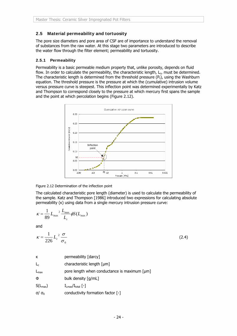


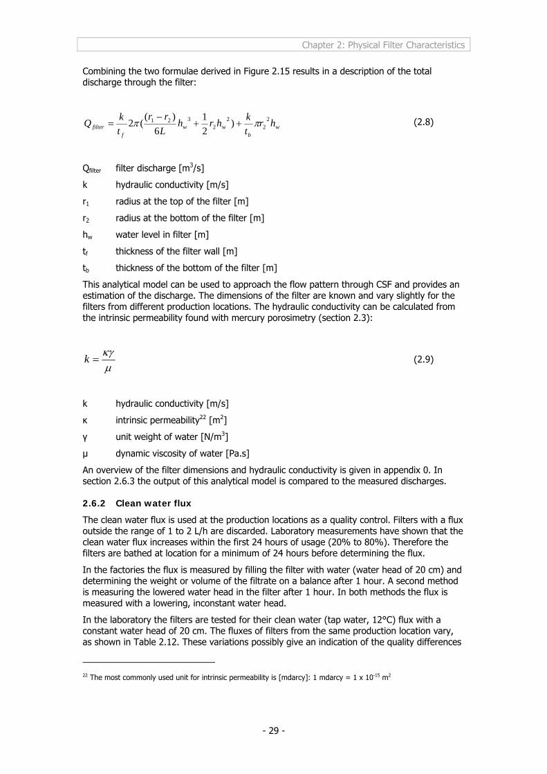


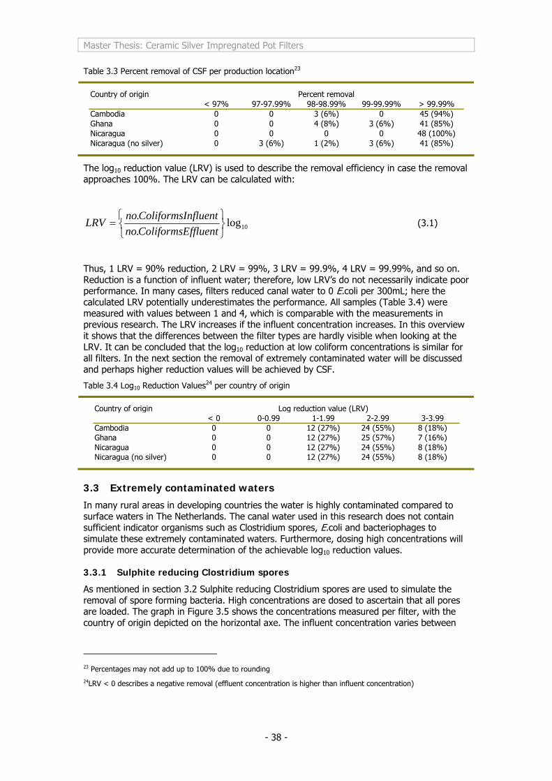


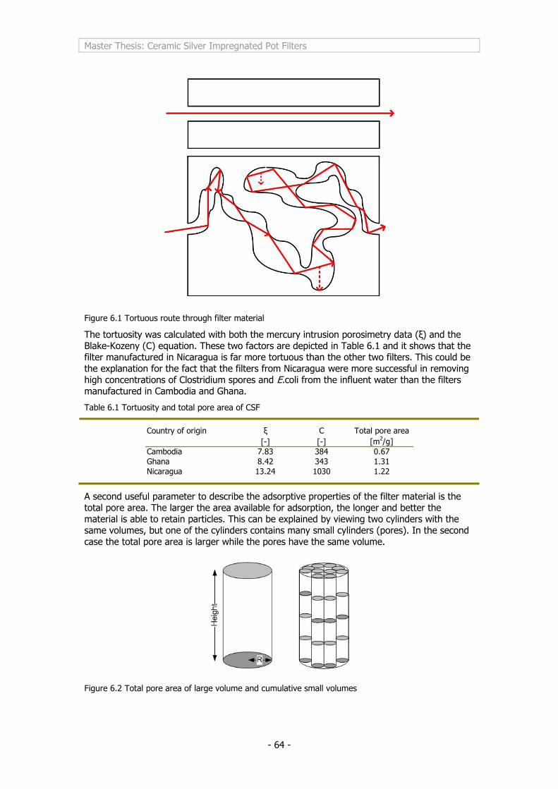


![[1019] 1) — 11-1 1989 AAR O-kJ¥ Ceramic Impregnated ...](https://static.documents.pub/doc/80x56/616f7ed737a0210bf80978bd/1019-1-11-1-1989-aar-o-kj-ceramic-impregnated-.jpg)
