Certicom ECC Challenge Abstract Certicom is pleased to present the Certicom Elliptic Curve Cryptosystem (ECC) Challenge. The first of its kind, the ECC Challenge has been developed to increase the industry’s understanding and appreciation for the difficulty of the elliptic curve discrete logarithm problem, and to encourage and stimulate further research in the security analysis of elliptic curve cryptosystems. It is our hope that the knowledge and experience gained from this Challenge will help confirm comparisons of the security levels of systems such as ECC, RSA and DSA that have been based primarily on theoretical considerations. We also hope it will provide additional information to users of elliptic curve public-key cryptosystems in terms of selecting suitable key lengths for a desired level of security. The Certicom ECC Challenge Defined The Challenge is to compute the ECC private keys from the given list of ECC public keys and associated system parameters. This is the type of problem facing an adversary who wishes to completely defeat an elliptic curve cryptosystem. There are two Challenge Levels: Level I, comprising 109-bit and 131-bit challenges; and Level II, comprising 163-bit, 191-bit, 239-bit and 359-bit challenges. The 109-bit challenges are considered feasible and could be solved within a few months, while the 131-bit challenges will require significantly more resources to solve. All Level II challenges are believed to be computationally infeasible. The Certicom ECC Challenge is preceded by some Exercises: 79-bit, 89-bit and 97-bit, respectively. These Exercises are feasible to complete given the current state of knowledge in algorithmic number theory and the computational resources available to the industry. Certicom believes that it is feasible that the 79-bit exercises could be solved in a matter of hours, the 89-bit exercises could be solved in a matter of days, and the 97-bit exercises in a matter of weeks using a network of 3000 computers. Participants can attempt solving the Exercise and Challenge sets using one or both of two finite fields. The first involves elliptic curves over the finite field F 2 m (the field having 2 m elements in it), and the second involves elliptic curves over the finite field F p (the field of integers modulo an odd prime p). The following sections present further background on the Certicom ECC Challenge, a mathematical overview of the elliptic curve discrete logarithm problem, a detailed technical description of the Challenge, the Challenge lists and corresponding prizes, and details on how to report solutions.
Transcript
Certicom ECC Challenge
Abstract Certicom is pleased to present the Certicom Elliptic Curve Cryptosystem (ECC) Challenge. The first of its kind, the ECC Challenge has been developed to increase the industry’s understanding and appreciation for the difficulty of the elliptic curve discrete logarithm problem, and to encourage and stimulate further research in the security analysis of elliptic curve cryptosystems.
It is our hope that the knowledge and experience gained from this Challenge will help confirm comparisons of the security levels of systems such as ECC, RSA and DSA that have been based primarily on theoretical considerations. We also hope it will provide additional information to users of elliptic curve public-key cryptosystems in terms of selecting suitable key lengths for a desired level of security. The Certicom ECC Challenge Defined
The Challenge is to compute the ECC private keys from the given list of ECC public keys and associated system parameters. This is the type of problem facing an adversary who wishes to completely defeat an elliptic curve cryptosystem.
There are two Challenge Levels: Level I, comprising 109-bit and 131-bit challenges; and Level II, comprising 163-bit, 191-bit, 239-bit and 359-bit challenges. The 109-bit challenges are considered feasible and could be solved within a few months, while the 131-bit challenges will require significantly more resources to solve. All Level II challenges are believed to be computationally infeasible.
The Certicom ECC Challenge is preceded by some Exercises: 79-bit, 89-bit and 97-bit, respectively. These Exercises are feasible to complete given the current state of knowledge in algorithmic number theory and the computational resources available to the industry. Certicom believes that it is feasible that the 79-bit exercises could be solved in a matter of hours, the 89-bit exercises could be solved in a matter of days, and the 97-bit exercises in a matter of weeks using a network of 3000 computers.
Participants can attempt solving the Exercise and Challenge sets using one or both of two finite fields. The first involves elliptic curves over the finite field F2m (the field having 2m elements in it), and the second involves elliptic curves over the finite field Fp (the field of integers modulo an odd prime p).
The following sections present further background on the Certicom ECC Challenge, a mathematical overview of the elliptic curve discrete logarithm problem, a detailed technical description of the Challenge, the Challenge lists and corresponding prizes, and details on how to report solutions.
ii
Contents
1 Introduction...........................................................................................1 1.1 Background ...........................................................................................................................1 1.2 Elliptic curve cryptosystems..................................................................................................1 1.3 Why have a challenge? ..........................................................................................................2
2 The Elliptic Curve Discrete Logarithm Problem (ECDLP) .................3 2.1 The discrete logarithm problem.............................................................................................3 2.2 Algorithms known for the ECDLP ........................................................................................3 2.3 Is there a subexponential-time algorithm for ECDLP?..........................................................6
3 The Challenge Explained .....................................................................6 3.1 Elliptic curves over F2m - format and examples.....................................................................7
3.1.1 The finite field F2m ........................................................................................................7 3.1.2 Elliptic curves over F2m .................................................................................................8 3.1.3 Format for challenge parameters (the F2m case) ............................................................9 3.1.4 Random elliptic curves and points (the F2m case)........................................................10
3.2 Elliptic curves over Fp - format and examples.....................................................................13 3.2.1 The finite field Fp ........................................................................................................13 3.2.2 Elliptic curves over Fp .................................................................................................13 3.2.3 Format for challenge parameters (the Fp case) ............................................................14 3.2.4 Random elliptic curves and points (the Fp case)..........................................................15
3.3 Further details about the challenge ......................................................................................17 3.4 Time estimates for exercises and challenges .......................................................................18
4 Exercise Lists and Challenge Lists...................................................19 4.1 Elliptic curves over F2m .......................................................................................................19
4.1.1 Exercises......................................................................................................................20 4.1.2 Level I challenges........................................................................................................20 4.1.3 Level II challenges ......................................................................................................20
4.2 Elliptic curves over Fp .........................................................................................................21 4.2.1 Exercises......................................................................................................................21 4.2.2 Level I challenges........................................................................................................21 4.2.3 Level II challenges ......................................................................................................21
5 Challenge Rules..................................................................................22 5.1 The Rules and Reporting a Solution....................................................................................22
5.1.1 Format of Submissions ................................................................................................22 5.1.2 Administration and Collection of Prizes......................................................................23
6 Status of the Certicom ECC Challenge.............................................24 6.1 Details of solved problems ..................................................................................................24
6.2 Status and estimates of ECC Challenge problems ...............................................................26 6.2.1 Elliptic Curves over F2m ..............................................................................................27 6.2.2 Elliptic curves over Fp .................................................................................................27
Since the invention of public-key cryptography in 1976 by Whitfield Diffie and Martin Hellman, numerous public-key cryptographic systems have been proposed. All of these systems rely on the difficulty of a mathematical problem for their security.
Over the years, many of the proposed public-key cryptographic systems have been broken, and many others have been demonstrated to be impractical. Today, only three types of systems should be considered both secure and efficient. Examples of such systems, classified according to the mathematical problem on which they are based, are:
1. Integer factorization problem (IFP): RSA and Rabin-Williams.
2. Discrete logarithm problem (DLP): the U.S. government’s Digital Signature Algorithm (DSA), the Diffie-Hellman and MQV key agreement schemes, the ElGamal encryption and signature schemes, and the Schnorr and Nyberg-Rueppel signature schemes.
3. Elliptic curve discrete logarithm problem (ECDLP): the elliptic curve analogue of the DSA (ECDSA), and the elliptic curve analogues of the Diffie-Hellman and MQV key agreement schemes, the ElGamal encryption and signature schemes, and the Schnorr and Nyberg-Rueppel signature schemes.
None of these problems have been proven to be intractable (i.e., difficult to solve in an efficient manner). Rather, they are believed to be intractable because years of intensive study by leading mathematicians and computer scientists around the world has failed to yield efficient algorithms for solving them. As more effort is expended over time in studying and understanding these problems, our confidence in the security of the corresponding cryptographic systems will continue to grow.
1.2 Elliptic curve cryptosystems
Elliptic curve cryptosystems (ECC) were proposed independently in 1985 by Victor Miller [Miller] and Neal Koblitz [Koblitz]. At the time, both Miller and Koblitz regarded the concept of ECC as mathematically elegant, however felt that its implementation would be impractical. Since 1985, ECC has received intense scrutiny from cryptographers, mathematicians, and computer scientists around the world. On the one hand, the fact that no significant weaknesses have been found has led to high confidence in the security of ECC. On the other hand, great strides have been made in improving the efficiency of the system, to the extent that today ECC is not just practical, but it is the most efficient public-key system known.
The primary reason for the attractiveness of ECC over systems such as RSA and DSA is that the best algorithm known for solving the underlying mathematical problem (namely, the ECDLP) takes fully exponential time. In contrast, subexponential-time algorithms are known for underlying mathematical problems on which RSA and DSA are based, namely the integer factorization (IFP) and the discrete logarithm (DLP) problems. This means that the algorithms for solving the ECDLP become
2
infeasible much more rapidly as the problem size increases than those algorithms for the IFP and DLP. For this reason, ECC offers security equivalent to RSA and DSA while using far smaller key sizes.
The attractiveness of ECC will increase relative to other public-key cryptosystems as computing
power improvements force a general increase in the key size. The benefits of this higher-strength-per-bit include:
• higher speeds,
• lower power consumption,
• bandwidth savings,
• storage efficiencies, and
• smaller certificates.
These advantages are particularly beneficial in applications where bandwidth, processing capacity, power availability, or storage are constrained. Such applications include:
• chip cards,
• electronic commerce,
• web servers,
• cellular telephones, and
• pagers.
1.3 Why have a challenge?
The objectives of this ECC challenge are the following:
1. To increase the cryptographic community’s understanding and appreciation of the difficulty of the ECDLP.
2. To confirm comparisons of the security levels of systems such as ECC, RSA and DSA that have been made based primarily on theoretical considerations.
3. To provide information on how users of elliptic curve public-key cryptosystems should select suitable key lengths for a desired level of security.
4. To determine whether there is any significant difference in the difficulty of the ECDLP for elliptic curves over F2m and the ECDLP for elliptic curves over Fp.
5. To determine whether there is any significant difference in the difficulty of the ECDLP for random elliptic curves over F2m and the ECDLP for Koblitz curves.
6. To encourage and stimulate research in computational and algorithmic number theory and, in particular, the study of the ECDLP.
3
2 The Elliptic Curve Discrete Logarithm Problem (ECDLP)
This section provides a brief overview of the state-of-the-art in algorithms known for solving the elliptic curve discrete logarithm problem. For more information, the reader is referred to Chapter 3 of the Handbook of Applied Cryptography [MVV].
2.1 The discrete logarithm problem
Roughly speaking, the discrete logarithm problem is the problem of “inverting” the process of exponentiation. The problem can be posed in a variety of algebraic settings. The most commonly studied versions of this problem are:
1. The discrete logarithm problem in a finite field (DLP): Given a finite field Fq and elements g, h ∈ Fq , find an integer l such that gl = h in Fq, provided that such an integer exists.
2. The elliptic curve discrete logarithm problem (ECDLP): Given an elliptic curve E defined over a finite field Fq , and two points P, Q ∈ E(Fq), find an integer l such that lP = Q in E, provided that such an integer exists.
On the surface, these two problems look quite different. In the first problem, “multiplicative”
notation is used: gl refers to the process of multiplying g by itself l times. In the second problem, “additive” notation is used: lP refers to the process of adding P to itself l times.
If one casts these notational differences aside, then the two problems are abstractly the same. What is intriguing about the two problems, however, is that the second appears to be much more difficult than the first. The fundamental reason for this is that the algebraic objects in the DLP (finite fields) are equipped with two basic operations: addition and multiplication of field elements. In contrast, the algebraic objects in the ECDLP (elliptic curves over finite felds) are equipped with only one basic operation: addition of elliptic curve points. The additional structure present in the DLP has led to the discovery of the index-calculus methods, which have a subexponential running time. Elliptic curves do not possess this additional structure, and for this reason noone has been able to apply the index-calculus methods to the ECDLP (except in very special and well-understood cases). This absence of subexponential-time algorithms for the ECDLP, together with efficient implementation of the elliptic curve arithmetic, is precisely the reason that elliptic curve cryptosystems have proven so attractive for practical use.
2.2 Algorithms known for the ECDLP
This section briefly overviews the algorithms known for the ECDLP. All of these algorithms take fully exponential time.
The following notations are used:
4
• q is the order of the underlying finite field.
• Fq is the underlying finite field of order q.
• E is an elliptic curve defined over Fq.
• E(Fq) is the set of points on E both of whose coordinates are in Fq , together with the point at infinity.
• P is a point in E(Fq).
• n is the large prime order of the point P.
• Q is another point in E(Fq).
The ECDLP is: Given q, E, P, n and Q, find an integer l, 0 ≤ l ≤ n – 1, such that lP = Q, provided that such an integer exists.
For the remainder of the discussion, we shall only consider instances of the ECDLP for which the integer l exists.
1. Naive exhaustive search. In this method, one simply computes successive multiples of P: P, 2P, 3P, 4P, ... until Q is obtained. This method can take up to n steps in the worst case.
2. Baby-step giant-step algorithm. This algorithm is a time-memory trade-off of the method of exhaustive search. It requires storage for about n points, and its running time is roughly n steps in the worst case.
3. Pollard’s rho algorithm. This algorithm, due to Pollard [Pollard], is a randomized version of the baby-step giant-step algorithm. It has roughly the same expected running time ( 2/nπ steps ) as the baby-step giant-step algorithm, but is superior in that it requires a negligible amount of storage. Gallant, Lambert and Vanstone [GLV], and Wiener and Zuccherato [WZ] showed how Pollard’s rho algorithm can be sped up by a factor of 2 . Thus the expected running time of Pollard’s rho method with this speedup is 2/nπ steps.
4. Distributed version of Pollard’s rho algorithm. Van Oorschot and Wiener [VW] showed how Pollard’s rho algorithm can be parallelized so that when the algorithm is run in parallel on m processors, the expected running time of the algorithm is roughly )2/( mnπ steps. That is, using m processors results in an m-fold speed-up.
This distributed version of Pollard’s rho algorithm is the fastest general-purpose algorithm known for the ECDLP.
5. Pohlig-Hellman algorithm. This algorithm, due to Pohlig and Hellman [PH], exploits the factorization of n, the order of the point P. The algorithm reduces the problem of recovering l to the problem of recovering l modulo each of the prime factors of n; the desired number l can then be recovered by using the Chinese Remainder Theorem.
5
The implications of this algorithm are the following. To construct the most difficult instance of the ECDLP, one must select an elliptic curve whose order is divisible by a large prime n. Preferably, this order should be a prime or almost a prime (i.e. a large prime n times a small integer h). The elliptic curves in the exercises and challenges posed here are all of this type.
6. Pollard’s lambda method. This is another randomized algorithm due to Pollard [Pollard]. Like Pollard’s rho method, the lambda method can also be parallelized with a linear speedup. The parallelized lambda method is slightly slower than the parallelized rho method [VW]. The lambda method is, however, faster in situations when the logarithm being sought is known to lie in a subinterval ],0[ b of ]1,0[ −n , where nb 39.0< [VW].
7. Multiple Algorithms R. Silverman and Stapleton [SS] observed that if a single instance of the ECDLP (for a given elliptic curve E and a base point P) is solved using Pollard’s rho method, then the work done in solving this instance can be used to speed up the solution of other instance of the ECDLP for the same curve E and base point P. More precisely, solving k instances of the ECDLP (for the same curve E and base point P) takes only k as much work as it does to solve one instance of the ECDLP. This analysis, however, does not take into account storage requirements.
Concerns that successive logarithms become easier can be addressed by ensuring that the elliptic parameters are chosen so that the first instance is infeasible to solve.
8. A special class of elliptic curves: supersingular curves. Menezes, Okamoto and Vanstone [MOV, Menezes] and Frey and Rück [FR] showed how, under mild assumptions, the ECDLP in an elliptic curve E defined over a finite field Fq can be reduced to the DLP in some extension field FqB for some B ≥ 1, where the number field sieve algorithm applies. The reduction algorithm is only practical if B is small — this is not the case for most elliptic curves, as shown by Balasubramanian and Koblitz [BK]. To ensure that this reduction algorithm does not apply to a particular curve, one only needs to check that n, the order of the point P, does not divide qB – 1 for all small B for which the DLP in FqB is tractable (1 ≤ B ≤ 2000/(log2 q) suffices).
For the very special class of supersingular elliptic curves, it is known that B ≤ 6. It follows that the reduction algorithm yields a subexponential-time algorithm for the ECDLP in supersingular curves. For this reason, supersingular curves are explicitly excluded from use in the ECDSA.
9. Another special class of elliptic curves: anomalous curves. Semaev [Semaev], Smart [Smart], Satoh and Araki [SA] showed that the ECDLP for the special class of anomalous elliptic curves is easy to solve. An anomalous elliptic curve over Fq is an ellipic curve over Fq which has exactly q points. The attack does not extend to any other classes of elliptic curves. Consequently, by verifying that the number of points on an elliptic does not equal the number of elements in the underlying field, one can easily ensure that the Smart-Satoh-Araki attack does not apply to a particular curve.
10. Curves defined over a small field Suppose that E is an elliptic curve defined over the finite field F2B. Gallant, Lambert and Vanstone [GLV], and Wiener and Zuccherato [WZ] showed how Pollard’s rho algorithm for computing elliptic curve logarithms in E(F2Bd) can be further sped up by a factor of d -- thus
6
the expected running time of Pollard’s rho method for these curves is 2// dnπ steps. For example, if E is a Koblitz curve, then Pollard’s rho algorithm for computing elliptic curve logarithms in E(F2m) can be sped up by a factor of m . This speedup should be considered when doing a security analysis of elliptic curves whose coefficients lie in a small subfield.
11. Curves defined over F2m, m Composite Galbraith and Smart [GS], expanding on earlier work by Frey [Frey], discuss how the Weil descent might be used to solve the ECDLP for elliptic curves defined over F2m where m is composite. More recently, Gaudry, Hess and Smart [GHS] refined these ideas to provide strong evidence that when m has a small divisor l (say, l=4), the ECDLP for elliptic curves defined over F2m can be solved faster than with Pollard’s rho algorithm.
It should be noted that some ECC standards, including the draft ANSI X9.63, explicitly exclude the use of elliptic curves over composite fields. The ANSI X9F1 committee also agreed in January 1999 to exclude the use of such curves in a forthcoming revision of ANSI X9.62.
2.3 Is there a subexponential-time algorithm for ECDLP?
Whether or not there exists a subexponential-time algorithm for the ECDLP is an important unsettled question, and one of great relevance to the security of ECC. It is extremely unlikely that anyone will ever be able to prove that no subexponential-time algorithm exists for the ECDLP. (Analogously, it is extremely unlikely that anyone will ever be able to prove that no polynomial-time (efficient) algorithm exists for the integer factorization and discrete logarithm problems.) However, much work has been done on the DLP over the past 24 years, and more specifically on the ECDLP over the past 16 years. No subexponential-time algorithm has been discovered for the ECDLP, confirming the widely-held belief that no such algorithm exists.
In particular, Miller [Miller] and J. Silverman and Suzuki [SS2] have given convincing arguments for why the most natural way in which the index-calculus algorithms can be applied to the ECDLP is most likely to fail.
Another very interesting line of attack on the ECDLP, called the xedni-calculus attack was recently
proposed by J. Silverman [Silverman]. However, it was subsequently shown by a team of researchers including J. Silverman (see Jacobson et al. [JKSST]) that the attack is virtually certain to fail in practice.
A summary of the work done on the ECDLP and further references can be found in the Certicom whitepaper [Certicom].
3 The Challenge Explained
This section gives an overview of some of the mathematics that is relevant to this challenge. The format for the challenge parameters presented in Section 4 is also explained.
7
For further background on finite fields, consult the books by McEliece [McEliece] and Lidl and Niederreiter [LN]. For further background on elliptic curves, consult the books by Koblitz [Koblitz3] and Menezes [Menezes].
3.1 Elliptic curves over F2m - format and examples
3.1.1 The finite field F2m
There are many ways to represent the elements of a finite field with 2m elements. The particular method used in this challenge is called a polynomial basis representation.
Let f (x) = xm + fm-1 xm-l + … + f2x2 + f1 x + f0 (where fi ∈ {0, 1} for i = 0, 1, . . ., m – 1) be an irreducible polynomial of degree m over F2. That is, f (x) cannot be factored as a product of two polynomials over F2 , each of degree less than m. The polynomial f (x) is called the reduction polynomial.
The finite field F2m is comprised of all polynomials over F2 of degree less than m:
The field element am-1 xm-l + am-2 xm-2 + …+ a1x + a0 is usually denoted by the binary string (am-1 am-2 … a1a0) of length m, so that
F2m = {(am-1 am-2 … a1a0) : ai ∈ {0, 1}}.
Thus the elements of F2m can be represented by the set of all binary strings of length m. The multiplicative identity element (1) is represented by the bit string (00. . .01), while the zero element (additive identity) is represented by the bit string of all 0’s. The following arithmetic operations are defined on the elements of F2m:
• Addition: If a = (am-1 am-2 … a1a0) and b = (bm-1 bm-2 … b1b0) are elements of F2m, then a + b = c = (cm-1 cm-2 … c1c0), where ci = (ai + bi) mod 2. That is, field addition is performed bitwise.
• Multiplication: If a = (am-1 am-2 … a1a0) and b = (bm-1 bm-2 … b1b0) are elements of F2m, then a • b = r = (rm-1 rm-2 … r1r0), where the polynomial rm-1 xm-l + rm-2 xm-2 + …+ r1x + r0 is the remainder when the polynomial
(am-1 xm-l + am-2 xm-2 + …+ a1x + a0) • (bm-1 xm-l + bm-2 xm-2 + …+ b1x + b0) is divided by f(x) over F2.
• Inversion: If a is a non-zero element in F2m, the inverse of a, denoted a-l, is the unique element c ∈ F2m for which a • c = 1.
Example (The finite field F24)
8
Let f (x) = x4 + x + 1 be the reduction polynomial. Then the elements of F24 are:
A (non-supersingular) elliptic curve E(F2m) over F2m defined by the parameters a, b ∈ F2m , b ≠ 0, is the set of all solutions (x, y), x, y ∈ F2m, to the equation
y2 + xy = x3 + ax2 + b, together with an extra point O, the point at infinity.
The set of points E(F2m) forms a group with the following addition rules:
1. O + O = O
2. (x, y) + O = O + (x, y) = (x, y) for all (x, y) ∈ E(F2m).
3. (x, y) + (x, x + y) = O for all (x, y) ∈ E(F2m) (i.e., the negative of the point (x, y) is –(x, y) = (x, x + y)).
4. (Rule for adding two distinct points that are not inverses of each other)
Let P = (xl, yl) ∈ E(F2m) and Q = (x2, y2) ∈ E(F2m) be two points such that x1 ≠ x2. Then P + Q = (x3, y3), where
,212
3 axxx ++++= λλ
and ,)( 13313 yxxxy +++= λ
. 12
12
xxyy
++=λ
5. (Rule for doubling a point)
Let P = (xl, yl) ∈ E(F2m) be a point with x1 ≠ 0. (If x1 = 0 then P = –P, and so 2P = O.) Then 2P = (x3, y3), where
,23 ax ++= λλ
and ,)1( 3213 xxy ++= λ
9
. 1
11
xyx +=λ
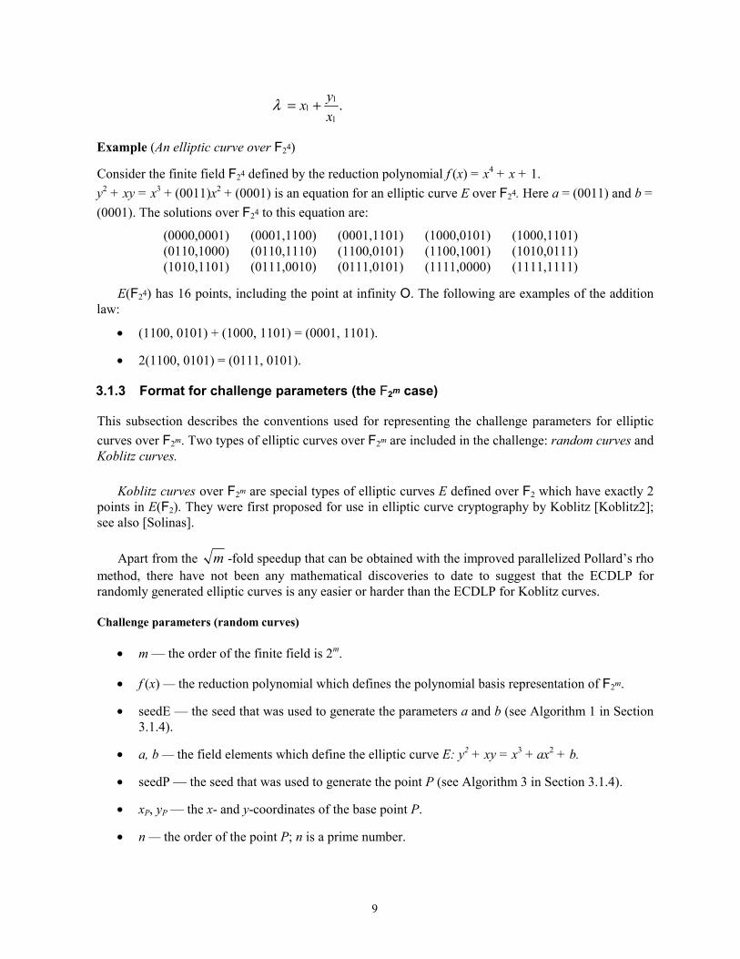
Example (An elliptic curve over F24)
Consider the finite field F24 defined by the reduction polynomial f (x) = x4 + x + 1. y2 + xy = x3 + (0011)x2 + (0001) is an equation for an elliptic curve E over F24. Here a = (0011) and b = (0001). The solutions over F24 to this equation are:
E(F24) has 16 points, including the point at infinity O. The following are examples of the addition law:
• (1100, 0101) + (1000, 1101) = (0001, 1101).
• 2(1100, 0101) = (0111, 0101).
3.1.3 Format for challenge parameters (the F2m case)
This subsection describes the conventions used for representing the challenge parameters for elliptic curves over F2m. Two types of elliptic curves over F2m are included in the challenge: random curves and Koblitz curves.
Koblitz curves over F2m are special types of elliptic curves E defined over F2 which have exactly 2 points in E(F2). They were first proposed for use in elliptic curve cryptography by Koblitz [Koblitz2]; see also [Solinas].
Apart from the m -fold speedup that can be obtained with the improved parallelized Pollard’s rho method, there have not been any mathematical discoveries to date to suggest that the ECDLP for randomly generated elliptic curves is any easier or harder than the ECDLP for Koblitz curves. Challenge parameters (random curves)
• m — the order of the finite field is 2m.
• f (x) — the reduction polynomial which defines the polynomial basis representation of F2m.
• seedE — the seed that was used to generate the parameters a and b (see Algorithm 1 in Section 3.1.4).
• a, b — the field elements which define the elliptic curve E: y2 + xy = x3 + ax2 + b.
• seedP — the seed that was used to generate the point P (see Algorithm 3 in Section 3.1.4).
• xP, yP — the x- and y-coordinates of the base point P.
• n — the order of the point P; n is a prime number.
10
• h — the co-factor h (the number of points in E(F2m) divided by n).
• seedQ — the seed that was used to generate the point Q (see Algorithm 3 in Section 3.1.4).
• xQ, yQ — the x- and y-coordinates of the public key point Q.
Challenge parameters (Koblitz curves)
• m — the order of the finite field is 2m.
• f (x) — the reduction polynomial which defines the polynomial basis representation of F2m.
• a, b — the field elements which define the elliptic curve E: y2 + xy = x3 + ax2 + b.
• seedP — the seed that was used to generate the point P (see Algorithm 3 in Section 3.1.4).
• xP, yP — the x- and y-coordinates of the base point P.
• n — the order of the point P; n is a prime number.
• h — the co-factor h (the number of points in E(F2m) divided by n).
• seedQ — the seed that was used to generate the point Q (see Algorithm 3 in Section 3.1.4).
• xQ, yQ — the x- and y-coordinates of the public key point Q.
Data formats
• Integers are represented in hexadecimal, the rightmost bit being the least significant bit. Example: The decimal integer 123456789 is represented in hexadecimal as 075BCD15.
• Field elements (of F2m) are represented in hexadecimal, padded with 0’s on the left. Example: Suppose m = 23. The field element a = x22 + x21 + x19 + x17 + x5 + 1 is represented in binary as (11010100000000000100001), or in hexadecimal as 006A0021.
• Seeds for generating random elliptic curves and random elliptic curve points (see Section 3.1.4) are 160-bit strings and are represented in hexadecimal.
3.1.4 Random elliptic curves and points (the F2m case)
This subsection describes the method that is used for verifiably selecting elliptic curves and points at random. The defining parameters of the elliptic curve or point are defined to be outputs of the one-way hash function SHA-1 (as specified in FIPS 180-1 [SHA-1]). The input seed to SHA-1 then serves as proof (under the assumption that SHA-1 cannot be inverted) that the elliptic curve or point were indeed generated at random.
The following notation is used: s = (m – 1)/160 and h = m –160 • s. Algorithm 1: Generating a random elliptic curve over F2m
Input: A field size q = 2m.
11
Output: A 160-bit bit string seedE and field elements a, b ∈ F2m which define an elliptic curve E over F2m.
1. Choose an arbitrary bit string seedE of length 160 bits.
2. Compute H = SHA-1(seedE), and let b0 denote the bit string of length h bits obtained by taking the h rightmost bits of H.
3. For i from 1 to s do: Compute bi = SHA-1((seedE + i) mod 2160).
4. Let b be the field element obtained by the concatenation of b0, b1, …, bs as follows: b = b0 b1 … bs.
5. If b = 0 then go to step 1.
6. Let a be an arbitrary element of F2m. (Note: For a fixed b, there are only 2 essentially different choices for a — other values of a give rise to isomorphic elliptic curves. Hence the choice of a is essentially without loss of generality.)
7. The elliptic curve chosen over F2m is E : y2 + xy = x3 + ax2 + b.
8. Output(seedE, a, b).
Algorithm 2: Verifying that an elliptic curve was randomly generated Input: A field size q = 2m, a bit string seedE of length 160 bits, and field elements a, b ∈ F2m which define an elliptic curve E : y2 + xy = x3 + ax2 + b over F2m. Output: Acceptance or rejection that E was randomly generated using Algorithm 1.
1. Compute H = SHA-1(seedE), and let b0 denote the bit string of length h bits obtained by taking the h rightmost bits of H.
2. For i from 1 to s do: Compute bi = SHA-1((seedE + i) mod 2160).
3. Let b’ be the field element obtained by the concatenation of b0, b1, …, bs as follows: b’ = b0 b1 … bs.
4. If b = b’ then accept; otherwise reject.
Algorithm 3: Generating a random elliptic curve point
Input: Field elements a, b ∈ F2m which define an elliptic curve E : y2 + xy = x3 + ax2 + b over F2m. The order of E(F2m) is n • h, where n is a prime. Output: A bit string seedP, a field element yU, and a point P ∈ E(F2m) of order n.
1. Choose an arbitrary bit string seedE of length 160 bits.
12
2. Compute H = SHA-1(seedP), and let x0 denote the bit string of length h bits obtained by taking the h rightmost bits of H.
3. For i from 1 to s do: Compute xi = SHA-1((seedP + i) mod 2160).
4. Let xU be the field element obtained by the concatenation of x0, x1, …, xs as follows: xU = x0 x1 … xs.
5. If the equation baxxyxy UUU ++=+ 232 does not have a solution y ∈ F2m, then go to step 1.
6. Select an arbitrary solution yU ∈ F2m to the equation baxxyxy UUU ++=+ 232 . (Note: this equation will have either 1 or 2 distinct solutions. Hence the choice of yU is essentially without loss of generality.)
7. Let U be the point (xU, yU).
8. Compute P = hU.
9. If P = O then go to step 1.
10. Output(seedP, yU, P).
Algorithm 4: Verifying that an elliptic curve point was randomly generated
Input: A field size q = 2m, field elements a, b ∈ F2m which define an elliptic curve E : y2 + xy = x3 + ax2 + b over F2m, a bit string seedP of length 160 bits, a field element yU ∈ F2m, and an elliptic curve point P = (xP, yP). The order of E(F2m) is n • h, where n is a prime. Output: Acceptance or rejection that P was randomly generated using Algorithm 3.
1. Compute H = SHA-1(seedP), and let x0 denote the bit string of length h bits obtained by taking the h rightmost bits of H.
2. For i from 1 to s do: Compute xi = SHA-1((seedP + i) mod 2160).
3. Let xU be the field element obtained by the concatenation of x0, x1, …, xs as follows: xU = x0 x1 … xs.
4. Let U be the point (xU, yU).
5. Verify that U satisfies the equation y2 + xy = x3 + ax2 + b.
6. Compute P’= hU.
7. If P ≠ P’then reject.
8. Accept.
13
3.2 Elliptic curves over Fp - format and examples
3.2.1 The finite field Fp
Let p be a prime number. The finite field Fp is comprised of the set of integers
{0, 1, 2, …, p –1}
with the following arithmetic operations:
• Addition: If a, b ∈ Fp, then a + b = r, where r is the remainder when a + b is divided by p and 0 ≤ r ≤ p – 1. This is known as addition modulo p.
• Multiplication: If a, b ∈ Fp, then a • b = s, where s is the remainder when a • b is divided by p and 0 ≤ s ≤ p – 1. This is known as multiplication modulo p.
• Inversion: If a is a non-zero element in Fp, the inverse of a modulo p, denoted a-1, is the unique integer c ∈ Fp for which a • c = 1.
Example ( The finite field F23) The elements of F23 are {0, 1, 2, . . ., 22}. Examples of the arithmetic operations in F23 are:
• 12 + 20 = 9.
• 8 • 9 = 3.
• 8–1 = 3. 3.2.2 Elliptic curves over Fp
Let p > 3 be a prime number. Let a, b ∈ Fp be such that 4a3 + 27b2 ≠ 0 in Fp. An elliptic curve E(Fp) over Fp defined by the parameters a and b is the set of all solutions (x, y), x, y ∈ Fp, to the equation
y2 = x3 + ax + b,
together with an extra point O, the point at infinity.
The set of points E(Fp) forms a group with the following addition rules:
1. O + O = O
2. (x, y) + O = O + (x, y) = (x, y) for all (x, y) ∈ E(Fp).
3. (x, y) + (x, – y) = O for all (x, y) ∈ E(Fp) (i.e., the negative of the point (x, y) is – (x, y) = (x, – y)).
4. (Rule for adding two distinct points that are not inverses of each other)
Let P = (xl, yl) ∈ E(Fp) and Q = (x2, y2) ∈ E(Fp) be two points such that x1 ≠ x2. Then P + Q = (x3, y3), where ,21
23 xxx −−= λ
and ,)( 1313 yxxy −−= λ
14
. 12
12
xxyy
−−=λ
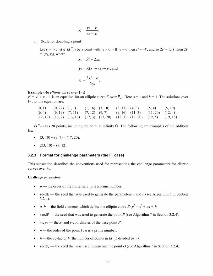
5. (Rule for doubling a point)
Let P = (xl, yl) ∈ E(Fp) be a point with y1 ≠ 0. (If y1 = 0 then P = –P, and so 2P = O.) Then 2P = (x3, y3), where ,2 1
23 xx −= λ
and ,)( 1313 yxxy −−= λ
.2
3 1
21
yax +=λ
Example (An elliptic curve over F23) y2 = x3 + x + 1 is an equation for an elliptic curve E over F23. Here a = 1 and b = 1. The solutions over F23 to this equation are:
E(F23) has 28 points, including the point at infinity O. The following are examples of the addition
law:
• (3, 10) + (9, 7) = (17, 20).
• 2(3, 10) = (7, 12).
3.2.3 Format for challenge parameters (the Fp case)
This subsection describes the conventions used for representing the challenge parameters for elliptic curves over Fp. Challenge parameters
• p — the order of the finite field; p is a prime number.
• seedE — the seed that was used to generate the parameters a and b (see Algorithm 5 in Section 3.2.4).
• a, b — the field elements which define the elliptic curve E: y2 = x3 + ax + b.
• seedP — the seed that was used to generate the point P (see Algorithm 7 in Section 3.2.4).
• xP, yP — the x- and y-coordinates of the base point P.
• n — the order of the point P; n is a prime number.
• h — the co-factor h (the number of points in E(Fp) divided by n).
• seedQ — the seed that was used to generate the point Q (see Algorithm 7 in Section 3.2.4).
15
• xQ, yQ — the x- and y-coordinates of the public key point Q.
Data formats
• Integers are represented in hexadecimal, the rightmost bit being the least significant bit. Example: The decimal integer 123456789 is represented in hexadecimal as 075BCD15.
• Field elements (of Fp) are represented as hexadecimal integers.
• Seeds for generating random elliptic curves and random elliptic curve points (see Section 3.2.4) are 160-bit strings and are represented in hexadecimal.
3.2.4 Random elliptic curves and points (the Fp case)
This subsection describes the method that is used for verifiably selecting elliptic curves and points at random. The defining parameters of the elliptic curve or point are defined to be outputs of the one-way hash function SHA-1 (as specified in FIPS 180-1 [SHA-1]). The input seed to SHA-1 then serves as proof (under the assumption that SHA-1 cannot be inverted) that the elliptic curve or point were indeed generated at random.
The following notation is used: t = log2 p, s = (t – 1)/160 and h = t –160 • s. Algorithm 5: Generating a random elliptic curve over Fp
Input: A field size p, where p is a prime. Output: A 160-bit bit string seedE and field elements a, b ∈ Fp which define an elliptic curve E over Fp.
1. Choose an arbitrary bit string seedE of length 160 bits.
2. Compute H = SHA-1(seedE), and let c0 denote the bit string of length h bits obtained by taking the h rightmost bits of H.
3. Let W0 denote the bit string of length h bits obtained by setting the leftmost bit of c0 to 0. (This ensures that r < p.)
4. For i from 1 to s do: Compute Wi = SHA-1((seedE + i) mod 2160).
5. Let W be the bit string obtained by the concatenation of W0, W1, …, Ws as follows: W = W0 W1 … Ws.
6. Let w1, w2,… , wt be the bits of W from leftmost to rightmost. Let r be the integer
∑ −== .21
iti
ti wr
7. Choose arbitrary integers a, b ∈ Fp such that r • b2 ≡ a3 (mod p). (Note: For a fixed r ≠ 0, there are only 2 essentially different choices for a and b — other values of a and b give rise to isomorphic elliptic curves. Hence the choice of a and b is essentially without loss of generality.)
8. If 4a3 + 27 b2 ≡ 0 (mod p) then go to step 1.
16
9. The elliptic curve chosen over Fp is E : y2 = x3 + ax + b.
10. Output(seedE, a, b).
Algorithm 6: Verifying that an elliptic curve was randomly generated
Input: A field size p (a prime), a bit string seedE of length 160 bits, and field elements a, b ∈ Fp which define an elliptic curve E : y2 = x3 + ax + b over Fp. Output: Acceptance or rejection that E was randomly generated using Algorithm 5.
1. Compute H = SHA-1(seedE), and let c0 denote the bit string of length h bits obtained by taking the h rightmost bits of H.
2. Let W0 denote the bit string of length h bits obtained by setting the leftmost bit of c0 to 0.
3. For i from 1 to s do: Compute Wi = SHA-1((seedE + i) mod 2160).
4. Let W’be the bit string obtained by the concatenation of W0, W1, …, Ws as follows: W’ = W0 W1 … Ws.
5. Let w1, w2,… , wt be the bits of W’ from leftmost to rightmost. Let r’ be the integer
∑ −== .2' 1
iti
ti wr
6. If r’• b2 ≡ a3 (mod p) then accept; otherwise reject.
Algorithm 7: Generating a random elliptic curve point
Input: Field elements a, b ∈ Fp which define an elliptic curve E : y2 = x3 + ax + b over Fp. The order of E(Fp) is n • h, where n is a prime. Output: A bit string seedP, a field element yU, and a point P ∈ E(Fp) of order n.
1. Choose an arbitrary bit string seedP of length 160 bits.
2. Compute H = SHA-1(seedP), and let c0 denote the bit string of length h bits obtained by taking the h rightmost bits of H.
3. Let x0 denote the bit string of length h bits obtained by setting the leftmost bit of c0 to 0.
4. For i from 1 to s do:
Compute xi = SHA-1((seedE + i) mod 2160).
5. Let xU be the bit string obtained by the concatenation of x0, x1, …, xs as follows:
xU = x0 x1 … xs.
6. If the equation baxxy UU ++= 32 does not have a solution y ∈ Fp, then go to step 1.
7. Select an arbitrary solution yU ∈ Fp to the equation baxxy UU ++= 32 . (Note: this equation will have either 1 or 2 distinct solutions. Hence the choice of yU is essentially without loss of generality.)
17
8. Let U be the point (xU, yU).
9. Compute P = hU.
10. If P = O then go to step 1.
11. Output(seedP, yU, P).
Algorithm 8: Verifying that an elliptic curve point was randomly generated
Input: A field size p (a prime), field elements a, b ∈ Fp which define an elliptic curve E : y2 = x3 + ax + b over Fp, a bit string seedP of length 160 bits, a field element yU ∈ Fp, and an elliptic curve point P = (xP, yP). The order of E(Fp) is n • h, where n is a prime. Output: Acceptance or rejection that P was randomly generated using Algorithm 7.
1. Compute H = SHA-1(seedP), and let c0 denote the bit string of length h bits obtained by taking the h rightmost bits of H.
2. Let x0 denote the bit string of length h bits obtained by setting the leftmost bit of c0 to 0.
3. For i from 1 to s do: Compute xi = SHA-1((seedE + i) mod 2160).
4. Let xU be the bit string obtained by the concatenation of x0, x1, …, xs as follows: xU = x0 x1 … xs.
5. Let U be the point (xU, yU).
6. Verify that U satisfies the equation y2 = x3 + ax + b.
7. Compute P’= hU.
8. If P ≠ P’then reject.
9. Accept.
3.3 Further details about the challenge
This subsection presents some more information about the challenge. Each problem posed is to compute the private key given the elliptic curve parameters, the base point P of order n, and the public key point Q. The private key is the unique integer l, 0 ≤ l ≤ n - 1, such that Q = lP. Each problem is therefore an instance of the elliptic curve discrete logarithm problem (ECDLP); see Section 2.
With the exception of the Koblitz curves, all elliptic curves have been chosen randomly in a verifiable manner (see Sections 3.1.4 and 3.2.4) — anyone can verify that the elliptic curve parameters were indeed generated at random.
Another interesting feature of the challenge is that the points P and Q having order n were also chosen randomly in a verifiable manner (see Sections 3.1.4 and 3.2.4). This means that each particular private key l is presently unknown even to the creators of the challenge!! However, any alleged solution l' that is found to a challenge can easily be verified by checking that Q = l'P. The challenges presented
18
here therefore adhere to the philosophy expressed by Matt Blaze [Blaze] at Crypto '97 that the solutions to a challenge should be unknown to the creators at the outset of the challenge.
The problems have been separated into two categories:
(i) elliptic curves over F2m, and
(ii) elliptic curves over Fp.
There have not been any mathematical discoveries to date to suggest that the ECDLP for elliptic curves over F2m is any easier or harder than the ECDLP for elliptic curves over Fp.
For each of these categories, the problems have been further divided into three sub-categories:
(i) Exercises,
(ii) Level I Challenges, and
(iii) Level II Challenges.
These are distinguished by the size of the parameter n, the prime order of the base point P. As the size of n increases, the problem is expected to become harder. By a k-bit challenge, we shall mean a challenge whose parameter n has bitlength k. 3.4 Time estimates for exercises and challenges
This subsection provides a very rough estimate for the time to solve a k-bit challenge with parameter n. These estimates are for software implementations; we do not assume that any special hardware for parallelized Pollard rho attacks is used.
Recall from Section 2.2 that the distributed version of Pollard’s rho algorithm using M processors takes approximately Mn /2/π steps. Here, each “step” is an elliptic curve addition or double together with some rho-method specific operations such as evaluations of hash functions and/or a membership test. Also recall from Section 2.2 that for binary anomalous curves (Koblitz curves) over F2m, the number of iterations can be reduced up to a factor of m2 , and for all other curves up to a factor of 2 .
Thus, if a computer can perform l operations per second, then the number of computer days required
before a discrete logarithm is found is expected to be roughly
Mml
nMmn
l×≈×
×××−510
22460601 π machine days
in the case of binary anomalous curves over F2m, and
lMn
Mn
l×≈×
×××−510
22460601 π
machine days
for all other curves.
19
To illustrate this, consider solving an instance of the ECDLP over F289 with n ≈ 289. A fast implementation of elliptic curve operations on a widely available computer, say a Pentium 100, may perform 16000 iterations per second for a curve over F289. Thus such an implementation would require
MM
1555016000
21089
5 ≈×
×− machine days
to find a single discrete logarithm. So, for example, one such machine running 24 hours a day would require 15550 days. A network of 3000 such machines would require about 5 days.
When estimating the challenge problems, we also take into account that the iterations scale quadratically on the number of machine words required by the field. We assume that we work with a 32-bit machine. Then, for example, a 109-bit field requires 4 machine words while a 89-bit field requires only 3 machine words. This means that each iteration in a 109-bit field should cost (4/3)2 as much. Hence, a Pentium 100 can perform about 900016000)4/3( 2 =×=l iterations per secod for a curve
over F2109. For a curve over a 89-bit prime field, we estimate that a Pentium 100 can perform about l = 48000
iterations per second. For a Koblitz curve over F289, we estimate that a Pentium 100 can perform about l=24000 iterations per second. Here we assume that iterations are done on orbits of points rather that on points. This slightly increases the time needed for one iteration while it considerably reduces the expected number of iterations.
The 109-bit Level I challenges are feasible using a very large network of computers. The 131-bit
Level I challenges are expected to be infeasible against realistic software and hardware attacks, unless of course, a new algorithm for the ECDLP is discovered.
The Level II challenges are infeasible given today’s computer technology and knowledge. The
elliptic curves for these challenges meet the stringent security requirements imposed by existing and forthcoming ANSI banking standards [X962, X963].
An implementation report of the Pollard rho algorithm for solving the ECDLP can be found in
[HMV]. An implementation report of the solution of some of the exercises can be found in [Escott]. The estimates are included in the tables in section 6.2.
4 Exercise Lists and Challenge Lists
4.1 Elliptic curves over F2m
In the following tables, ECC2-k denotes that the exercise or challenge is over a field F2m, and that the parameter n has bitlength k. Furthermore, ECC2K-k denotes that the elliptic curve used is a Koblitz curve (see Section 3.1.3), rather than a randomly generated curve.
20
For a description of the format of the challenge parameters, see Section 3.1.3. For further details about the challenge, see Section 3.3. The time estimates for each exercise and challenge were derived as in Section 3.4.
Using these timings, it is expected that the 79-bit exercise could be solved in a matter of hours, the 89-bit exercise could be solved in a matter of days, and the 97-bit exercise in a matter of weeks using a network of 3000 computers.
The 109-bit Level I challenge is feasible using a very large network of computers. The 131-bit Level
I challenge is expected to be infeasible against realistic software and hardware attacks, unless of course a new algorithm for the ECDLP is discovered.
The Level II challenges are infeasible given today’s computer technology and knowledge. The elliptic curves for these challenges meet the stringent security requirements imposed by existing and forthcoming ANSI banking standards [X962, X963]. 4.1.1 Exercises
Exercise Field size (in bits)
Estimated number of machine days
Prize (US$)
ECC2-79 79 352 Handbook of Applied Cryptography & Maple V software
ECC2-89 89 11278 Handbook of Applied Cryptography & Maple V software
ECC2K-108 109 1.3 x 10⁶ $ 10,000 ECC2-109 109 2.1 x 10⁷ $ 10,000 ECC2K-130 131 2.7 x 10⁹ $ 20,000 ECC2-131 131 6.6 x 10¹⁰ $ 20,000
4.1.3 Level II challenges
Challenge Field size (in bits)
Estimated number of machine days
Prize (US$)
ECC2-163 163 6.2 x 10¹⁵ $ 30,000 ECC2K-163 163 3.2 x 10¹⁴ $ 30,000 ECC2-191 191 1.0 x 10²⁰ $ 40,000 ECC2-238 239 2.1 x 1027 $ 50,000 ECC2K-238 239 9.2 x 1025 $ 50,000
21
ECC2-353 359 1.3 x 1045 $ 100,000 ECC2K-358 359 2.8 x 1044 $ 100,000
4.2 Elliptic curves over Fp
In the following tables, ECCp-k denotes that the exercise or challenge is over a field Fp (p prime), and that the parameter n has bitlength k.
For a description of the format of the challenge parameters, see Section 3.2.3. For further details about the challenge, see Section 3.3. The time estimates for each exercise and challenge were derived as in Section 3.4.
Using these timings, it is expected that the 79-bit exercise could be solved in a matter of hours, the 89-bit exercise could be solved in a matter of days, and the 97-bit exercise in a matter of weeks using a network of 3000 computers.
The 109-bit Level I challenge is feasible using a very large network of computers. The 131-bit Level I challenge is expected to be infeasible against realistic software and hardware attacks, unless of course a new algorithm for the ECDLP is discovered.
The Level II challenges are infeasible given today’s computer technology and knowledge. The elliptic curves for these challenges meet the stringent security requirements imposed by existing and forthcoming ANSI banking standards [X962, X963]. 4.2.1 Exercises
Exercise Field size (in bits)
Estimated number of machine days
Prize (US$)
ECCp-79 79 146 Handbook of Applied Cryptography & Maple V software
ECCp-89 89 4360 Handbook of Applied Cryptography & Maple V software
ECCp-97 97 71982 $ 5,000 4.2.2 Level I challenges
Challenge Field size (in bits)
Estimated number of machine days
Prize (US$)
ECCp-109 109 9.0 x 10⁶ $ 10,000 ECCp-131 131 2.3 x 10¹⁰ $ 20,000
4.2.3 Level II challenges
Challenge Field size (in bits)
Estimated number of machine days
Prize (US$)
ECCp-163 163 2.3 x 10¹⁵ $ 30,000
22
ECCp-191 191 4.8 x 10¹⁹ $ 40,000 ECCp-239 239 1.4 x 1027 $ 50,000 ECCp-359 359 3.7 x 1045 $ 100,000
5 Challenge Rules
5.1 The Rules and Reporting a Solution
Each exercise and challenge in the Exercise and Challenge Lists is based on the problem of computing the ECC private key from the given ECC public key and associated system parameters. An individual or group of individuals reporting a solution must also provide a full explanation of how that solution was reached. No reported solutions will be accepted without a detailed explanation of the steps taken and calculations made to find an ECC private key. As noted in Section 3.3, each particular private key is presently unknown even to the creators of the Certicom ECC Challenge. Unique to all algorithms based on the discrete logarithm problem, a supposed ECC public key can be validated to ensure it conforms to the arithmetic requirements of a public-key. This validation is 100%. When an ECC public key is validated, it is known that a private key for the public key can logically exist. This capability of key validation is used in the Certicom ECC Challenge. The proposed solution must be sent via email to Certicom Corp., following the Format of Submissions specified in Section 5.1.1. The correct solution for an Exercise or Challenge will be the one that was received first by Certicom Corp. and checked by an independent, third-party appointed by Certicom. Certicom Corp. reserves the right to change the contest rules at any time at its sole discretion, without notice, including the right to change or extend the challenge lists, to change the prize amounts, and/or to terminate the contest. While Certicom has appointed an independent, third-party to check the solutions, Certicom Corp. is the sole arbiter and administrator for this contest. Certicom’s judgement in all matters is final. Queries on the Certicom ECC Challenge can be addressed to: Certicom ECC Challenge Administrator Certicom Corp. 5520 Explorer Drive Mississauga, Ontario Canada L4W 5L1 For further information concerning the Certicom ECC Challenge, email inquiries can be sent to [email protected]. For news of the latest developments in the Certicom ECC Challenge, check Certicom’s web site at www.certicom.com.
5.1.1 Format of Submissions
All solution submissions for any of the exercises or challenges must be sent by email to [email protected]. The report of a solution should clearly state that the submission is being made
for the Certicom ECC Challenge. The body of the email message must contain the following information, titled with the respective headers:
• Name: name(s) of the person or people making the submission;
• Address: mailing address of the reporting party;
• Email: email address of the reporting party;
• Phone: telephone number and area code of the reporting party;
• Exercise or Challenge: specific exercise or challenge for which the submission is being made (see Sections 4.1 and 4.2 for exercise and challenge tables);
• Solution: actual private key value being submitted;
• Method: steps and computations taken to calculate the private key, and any other relevant information such as the estimated time taken to calculate the solution and the type of machine(s) used in the computations.
After each field, there must be the word “DONE” to indicate the end of the submission. The “name”, “address”, “email”, “phone”, “exercise or challenge”, “solution”, and “method” fields must be present in every submission. Without these fields, the solution report will be rejected. While it is preferred that the information fields be separated as specified above, information from two fields can be merged into one. Each field must start on a new line. If more than one person is reporting a solution in a group, the names of each individual along with their corresponding address, email and phone number should be contained in separate fields in alphabetical order. 5.1.2 Administration and Collection of Prizes
The first person or party to report the correct solution for any exercise or challenge, complete with the methodology and steps used to discover that solution, will win the prize for that particular exercise or challenge he/she has solved. An organized group of individuals reporting a solution will be treated the same as one person reporting a solution, in that only one cash prize will be awarded to the group with the correct solution, reported as specified in section 5.1.1. The prize shall be administered so that it is divided evenly among all members of that group. In several instances, there are two exercises or challenges with the same field size (e.g. 97-bit exercise) and the same corresponding cash prize, but are based on one of two finite fields—elliptic curves over the finite field F2
m and elliptic curves over the finite field Fp. These exercises and challenges have different solutions and the corresponding prizes will be awarded accordingly. Therefore, should the correct solution be properly reported for the Exercise ECC2-97 (97-bit field size over the field F2
m), the ECC2K-97 exercise (97-bit field size over the field Fp) would still be available to solve and the cash prize available for award to the person(s) with the correct solution.
24
6 Status of the Certicom ECC Challenge
The challenge was released on November 6, 1997, at 1 p.m. EST. The table below shows which problems have been solved so far. Here, the date given as end date indicates the day of submission of the solution to Certicom.
Challenge End Date Elliptic Curve Operations
Iterations per second*
Machine Days*
ECC2-79 Dec. 16, 1997 1.7 x 10¹² 170000 116 ECC2-89 Feb. 9, 1998 1.8 x 10¹³ 187000 1114 ECC2K-95 May 21, 1998 2.2 x 10¹³ 149000 1709 ECC2-97 Sep. 22, 1999 1.2 x 10¹⁴ 227000 6118 ECC2K-108 Apr 4, 2000 2.3 x 10¹⁵ 160364 166000 ECCp-79 Dec. 6, 1997 1.4 x 10¹² 314000 52 ECCp-89 Jan. 12, 1998 2.4 x 10¹³ 388000 716 ECCp-97 Mar. 18, 1998 2.0 x 10¹⁴ 361000 6412 *on 500 MHz Digital Alpha workstation running Linux
Since the algorithms for all problems were based on Pollard’s rho method [Pollard], the number of elliptic curve operations indicated above is the same as the number of iterations in the rho method.
The fourth column of the table indicates how many such iterations per seconds were performed by
the challenge solvers’ routines on a 500 MHz Alpha workstation, which is a typical machine used in the computations. Here, any speedup going from smaller to larger field sizes is due to code optimization. The penultimate column shows how many machine days on a 500 MHz Alpha would have been necessary if the whole computation had been performed on a single such machine running 24 hours a day.
All problems except the ECCp-97 problem were solved using the parallelized Pollard rho method due
to van Oorschot and Wiener [VW]; for the ECCp-97 problem, a parallelized Brent-type cycle-finding algorithm was used. Furthermore, for the ECC2K-95 and ECC2K-108 problem the number of iterations was reduced since the iterations were performed on orbits rather than on individual points.
For an implementation report of the solution of some of the exercises, see [Escott].
6.1 Details of solved problems
6.1.1 ECC2-79
• Solution: logPQ = 3AA0 68A09F1E D21E2582 • Date: 16 Dec 1997 • Communicated by: Robert J. Harley ([email protected]) • Who solved it: group of about 20 people • Method: parallelized Pollard rho method:
• Date: 9 Feb 1998 • Communicated by: Robert J. Harley ([email protected]) • Who solved it: group of about 70 people • Method: parallelized Pollard rho method:
• Solution: logPQ = 7A4249BA 547313AF 5D482092 • Date: 21 May 1998 • Communicated by: Robert J. Harley ([email protected]) • Who solved it: group of 47 people • Method: parallelized Pollard rho method, with speedup by introduction of equivalence classes:
• Roughly 21 600 000 000 000 iterations • 74 268 distinguished points • equivalence classes: the orbits under the involution [-1] and the Frobenius endomorphism
]2/)71[( −+− (= clusters of 194 points).
6.1.4 ECC2-97
• Solution: logPQ = CF765639 D6B81943 FD89D60F • Date: 22 Sep 1999 • Communicated by: Robert J. Harley ([email protected]) • Who solved it: group of 195 people • Method: parallelized Pollard rho method:
• Solution: logPQ = 0256 F98379F7 214306BE 5BE678FD • Date: 4 Apr 2000 • Communicated by: Robert J. Harley ([email protected]) • Who solved it: group of about 1300 people • Method: parallelized Pollard rho method with speedup:
• 2.3 x 10¹⁵ iterations • 2.05 million distinguished points
6.1.6 ECCp-79
• Solution: logPQ = 1387 56822DD5 FB093766 • Date: 6 Dec 1997 • Communicated by: Robert J. Harley ([email protected]) • Who solved it: W. Baisley and R.J. Harley • Method: Pollard’s rho method, parallelized Brent-type cycle-finding algorithm:
• Solution: logPQ = 0113C284 D9BD7B58 BCA30C67 • Date: 12 Jan 1998 • Communicated by: Robert J. Harley ([email protected]) • Who solved it: group of 57 people • Method: parallelized Pollard rho method:
• Solution: logPQ = 01 6C86AA7C ACF69F1D D28B3E2F • Date: 18 Mar 1998 • Communicated by: Dimitris Tsapakidis ([email protected]) • Who solved it: group of 588 people • Method: parallelized Pollard rho method:
• About 2.0 x 10¹⁴ iterations • 186 364 distinguished points
6.2 Status and estimates of ECC Challenge problems
Here we list the tables of both solved and unsolved problems, their status and Certicom’s estimate of computation required for solution. For a detailed explanation of the estimates, please refer to section 3.4.
Level II Challenges Estimated number of Challenge Start Date End Date Number of
Elliptic Curve Operations taken
Elliptic Curve Operations
Iterations per second*
Machine days*
ECC2-163 Nov. 6, 1997 2.1x1024 4000 6.2x10¹⁵
ECC2K-163 Nov. 6, 1997 1.7x10²³ 6000 3.2x10¹⁴
ECC2-191 Nov. 6, 1997 3.5x1028 4000 1.0x10²⁰
ECC2-238 Nov. 6, 1997 4.2x1035 2250 2.1x1027
ECC2K-238 Nov. 6, 1997 2.7x1034 3375 9.2x1025
ECC2-353 Nov. 6, 1997 1.1x1053 1000 1.3x1045
ECC2K-358 Nov. 6, 1997 3.6x1052 1500 2.8x1044
*Estimation based on a Pentium 100 6.2.2 Elliptic curves over Fp
28
Exercises Estimated number of Challenge Start Date End Date Number of
Elliptic Curve Operations taken
Elliptic Curve Operations
Iterations per second*
Machine days*
ECCp-79 Nov. 6, 1997 Dec. 6, 1997 1.4x10¹² 6.1x10¹¹ 48000 146 ECCp-89 Nov. 6, 1997 Jan. 12, 1998 2.4x10¹³ 1.8x10¹³ 48000 4360 ECCp-97 Nov. 6, 1997 Mar. 18, 1998 2.0x10¹⁴ 3.0x10¹⁴ 48000 71982 Level I Challenges Estimated number of Challenge Start Date End Date Number of
Elliptic Curve Operations taken
Elliptic Curve Operations
Iterations per second*
Machine days*
ECCp-109 Nov. 6, 1997 2.1x10¹⁶ 27000 9.0x10⁶
ECCp-131 Nov. 6, 1997 3.5x10¹⁹ 17820 2.3x10¹¹
Level II Challenges Estimated number of Challenge Start Date End Date Number of
Elliptic Curve Operations taken
Elliptic Curve Operations
Iterations per second*
Machine days*
ECCp-163 Nov. 6, 1997 2.4x1024 12000 2.3x10¹⁵
ECCp-191 Nov. 6, 1997 4.9x1028 12000 4.8x10¹⁹
ECCp-239 Nov. 6, 1997 8.2x1035 6750 1.4x1027
ECCp-359 Nov. 6, 1997 9.6x1053 3000 3.7x1045
*Estimation based on a Pentium 100
29
7 References
[BK] R. Balasubramanian and N. Koblitz, “The improbability that an elliptic curve has
subexponential discrete log problem under the Menezes-Okamoto-Vanstone algorithm”, Journal of Cryptology, 11 (1998), 114-145.
[Blaze] M. Blaze, “A better DES challenge”, presentation at the rump session at Crypto ‘97. [Certicom] Certicom Corp. white paper, “Remarks on the security of the elliptic curve
cryptosystem”, September 1997. Available from http://www.certicom.com
[Escott] A. Escott, J. Sager, A. Selkirk and D. Tsapakidis, “Attacking elliptic curve cryptosystems using the parallel Pollard rho method”, Cryptobytes – The Technical Newsletter of RSA Laboratories, volume 4, number 2, Winter 1999, 15-19. Also available at http://www.rsasecurity.com/
[FR] G. Frey and H. Rück, “A remark concerning m-divisibility and the discrete logarithm in the divisor class group of curves”, Mathematics of Computation, volume 62, pages 865-874, 1994.
[Frey] G. Frey, “How to disguise an elliptic curve (Weil descent)”, talk at ECC ’98. Slides available at http://www.cacr.math.uwaterloo.ca
[GLV] R. Gallant, R. Lambert and S. Vanstone, “Improving the parallelized Pollard lambda search on binary anomalous curves”, to appear in Mathematics of Computation.
[GS] S. Galbraith and N. Smart, “A cryptographic application of Weil descent”, Codes and Cryptography, Lecture Notes in Computer Science, 1746 (1999), Springer-Verlag, 865-874.
[HMV] G. Harper, A. Menezes and S. Vanstone, “Public-key cryptosystems with very small key lengths”, Advances in Cryptology - EUROCRYPT ‘92, Lecture Notes in Computer Science, volume 658, Springer-Verlag, pages 163-173, 1993.
[JKSST] M. Jacobson, N. Koblitz, J. Silverman, A. Stein and E. Teske, “Analysis of the xedni calculus attack”, Designs, Codes and Cryptography, to appear, 2000. Also available at http://www.cacr.math.uwaterloo.ca/
[Koblitz] N. Koblitz, “Elliptic curve cryptosystems”, Mathematics of Computation, volume 48, pages 203-209, 1987.
[Koblitz2] N. Koblitz, “CM-curves with good cryptographic properties”, Advances in Cryptology -CRYPTO ‘91, Lecture Notes in Computer Science, volume 576, Springer-Verlag, pages 279-287, 1992.
[Koblitz3] N. Koblitz, A Course in Number Theory and Cryptography, Springer-Verlag, 2nd edition, 1994.
[LN] R. Lidl and H. Niederreiter, Introduction to Finite Fields and their Applications, Cambridge University Press, 1994.
[MVV] A. Menezes, P. van Oorschot and S. Vanstone, Handbook of Applied Cryptography, CRC Press, 1997.
[MOV] A. Menezes, T. Okamoto and S. Vanstone, “Reducing elliptic curve logarithms to logarithms in a finite field”, IEEE Transactions on Information Theory, volume 39, pages 1639-1646, 1993.
[Miller] V. Miller, “Uses of elliptic curves in cryptography”, Advances in Cryptology - CRYPTO ‘85, Lecture Notes in Computer Science, volume 218, Springer-Verlag, pages 417-426, 1986.
[PH] S. Pohlig and M. Hellman, “An improved algorithm for computing logarithms over GF(p) and its cryptographic significance”, IEEE Transactions on Information Theory, volume 24, pages 106-110, 1978.
[Pollard] J. Pollard, “Monte Carlo methods for index computation mod p”, Mathematics of Computation, volume 32, pages 918-924, 1978.
[SHA-1] FIPS 180-1, “Secure hash standard”, Federal Information Processing Standards Publication 180-1, U.S. Department of Commerce/N.I.S.T., April 1995.
[SA] T. Satoh and K. Araki, “Fermat quotients and the polynomial time discrete log algorithm for anomalous elliptic curves”, preprint, 1997.
[Semaev] I. Semaev, “Evaluation of discrete logarithms in a group of p-torsion points of an elliptic curve in characteristic p”, Mathematics of Computation, 67 (1998), 353-356.
[Silverman] J. Silverman, “The xedni calculus and the elliptic curve discrete logarithm problem”, Designs, Codes and Cryptography, to appear, 2000. Also available at http://www.cacr.math.uwaterloo.ca/
[Smart] N. Smart, Announcement of an attack on the ECDLP for anomalous elliptic curves, 1997.
[Solinas] J. Solinas, “An improved algorithm for arithmetic on a family of elliptic curves”, Advances in Cryptology - CRYPTO ‘97, Lecture Notes in Computer Science, volume 1294, Springer-Verlag, pages 357-371, 1997.
[SS] R. Silverman and J. Stapleton, Contribution to ANSI X9F1 working group, 1997.
[SS2] J. Silverman and J. Suzuki, “elliptic curve discrete logarithms and the index calculus”, Advances in Cryptology – Asiacrypt ’98, Lecture Notes in Computer Science, 1514 (1999), Springer-Verlag, 110-125.
[VW] P. van Oorschot and M. Wiener, “Parallel collision search with cryptanalytic applications”, Journal of Cryptology, 12 (1999), 1-28.
[WZ] M. Wiener and R. Zuccherato, “Faster attacks on elliptic curve cryptosystems”, Selected Areas in Cryptography, Lecture Notes in Computer Science, 1556 (1999), Springer-Verlag, 190-200.
[X962] ANSI X9.62, “The elliptic curve digital signature algorithm (ECDSA)”, 1999.
[X963] ANSI X9.63, “Elliptic curve key agreement and transport protocols”, draft standard, 1997.