CFAST - Consolidated Fire and Smoke Transport (Version 7 ...

NIST Technical Note 1889v5

CFAST – Consolidated Fireand Smoke Transport

(Version 7)Volume 5: CFAST Fire Data Generator

(CData)

Paul A. RenekeRichard D. Peacock

Stanley W. GilbertThomas G. Cleary

This publication is available free of charge from: https://doi.org/10.6028/NIST.TN.1889v5

NIST Technical Note 1889v5

CFAST – Consolidated FireAnd Smoke Transport

(Version 7)Volume 5: CFAST Fire Data Generator

(CData)

Paul A. RenekeRichard D. Peacock

Thomas G. ClearyFire Research Division, Engineering Laboratory, Gaithersburg, Maryland

Stanley W. GilbertOffice of Economics, Engineering Laboratory, Gaithersburg, Maryland


June 2021CFAST Version 7.6.0

GIT Revision: unknown

UN

ITE

DSTATES OF AM

ER

ICA

DE

PARTMENT OF COMMERC

E

U.S. Department of CommerceGina M. Raimondo, Secretary

National Institute of Standards and TechnologyJames K. Olthoff, Performing the Non-Exclusive Functions and Duties of the Under Secretary of Commerce

for Standards and Technology & Director, National Institute of Standards and Technology

Preface

This document provides documentation for creating and running Monte Carlo simulations with theConsolidated Fire And Smoke Transport (CFAST) model using the CFAST Fire Data Generator(CData). The method follows the general framework set forth in the “Standard Guide for Eval-uating the Predictive Capability of Deterministic Fire Models,” ASTM E 1355 [1]. Instructionsfor using CFAST are contained in a separate user’s guide, and model assessment information iscontained in a separate verification and validation guide.

iii

iv

Disclaimer

The US Department of Commerce makes no warranty, expressed or implied, to users of CFAST,and accepts no responsibility for its use. Users of CFAST assume sole responsibility under Federallaw for determining the appropriateness of its use in any particular application; for any conclusionsdrawn from the results of its use; and for any actions taken or not taken as a result of analysisperformed using these tools.

Users are warned that CFAST is intended for use only by those competent in the fields offluid dynamics, thermodynamics, heat transfer, combustion, and fire science, and is intended onlyto supplement the informed judgment of the qualified user. The software package is a computermodel that may or may not have predictive capability when applied to a specific set of factualcircumstances. Lack of accurate predictions by the model could lead to erroneous conclusionswith regard to fire safety. All results should be evaluated by an informed user.

Throughout this document, the mention of computer hardware or commercial software does notconstitute endorsement by the National Institute of Standards and Technology, nor does it indicatethat the products are necessarily those best suited for the intended purpose.

National Institute of Standards and Technology Technical Note 1889v5 Natl. Inst. Stand. Technol. Tech. Note 1889v5, 99 pages (June 2021)

CODEN: NTNOEF


v

vi

Acknowledgments

CFAST was originally developed by Walter Jones, formerly of NIST.Continuing support for CFAST is via internal funding at NIST. In addition, support is provided

by other agencies of the U.S. Federal Government, most notably the Nuclear Regulatory Commis-sion (NRC) and the Department of Energy (DOE). The NRC Office of Research has funded keyvalidation experiments, the preparation of the CFAST manuals, and the continuing developmentof sub-models that are of importance in the area of nuclear power plant safety. Special thanks toMark Salley and David Stroup for their support. Support to refine the software development andquality assurance process for CFAST has been provided by the DOE. The assistance of Subir Senand Debra Sparkman is gratefully acknowledged.

We also thank Dr. Wai Cheong Tam, Dr. Justin Williamson, and Nelson Bryner for theirreviews and corrections. Any remaining errors are ours.

vii

viii

Contents

Preface iii

Disclaimer v

Acknowledgments vii

1 Getting Started 11.1 Installation . . . . . . . . . . . . . . . . . . . . . . . . . . . . . . . . . . . . . . 21.2 Defining the Question and the Analysis . . . . . . . . . . . . . . . . . . . . . . . 2

1.2.1 Building Characteristics . . . . . . . . . . . . . . . . . . . . . . . . . . . . 31.2.2 Fire Scenarios . . . . . . . . . . . . . . . . . . . . . . . . . . . . . . . . . 8

2 Defining Data for Analysis, CData Inputs 92.1 Namelist MHDR . . . . . . . . . . . . . . . . . . . . . . . . . . . . . . . . . . . 92.2 Namelist MRND . . . . . . . . . . . . . . . . . . . . . . . . . . . . . . . . . . . 102.3 Namelist MFLD . . . . . . . . . . . . . . . . . . . . . . . . . . . . . . . . . . . 132.4 Namelist MFIR . . . . . . . . . . . . . . . . . . . . . . . . . . . . . . . . . . . . 162.5 Namelist MSTT . . . . . . . . . . . . . . . . . . . . . . . . . . . . . . . . . . . 212.6 Namelist OUTP . . . . . . . . . . . . . . . . . . . . . . . . . . . . . . . . . . . 22

3 Creating Multiple CFAST Runs 233.1 PreProcessor . . . . . . . . . . . . . . . . . . . . . . . . . . . . . . . . . . . . . 233.2 Running CFAST . . . . . . . . . . . . . . . . . . . . . . . . . . . . . . . . . . . 253.3 Generating Statistics . . . . . . . . . . . . . . . . . . . . . . . . . . . . . . . . . 26

3.3.1 Accumulator . . . . . . . . . . . . . . . . . . . . . . . . . . . . . . . . . . 263.3.2 Statistics . . . . . . . . . . . . . . . . . . . . . . . . . . . . . . . . . . . . 27

4 Examples 334.1 Example 1: Flashover in a compartment . . . . . . . . . . . . . . . . . . . . . . . 33

4.1.1 CData Inputs . . . . . . . . . . . . . . . . . . . . . . . . . . . . . . . . . 344.1.2 Results . . . . . . . . . . . . . . . . . . . . . . . . . . . . . . . . . . . . . 35

4.2 Example 2: Impact of smoke detector interconnection . . . . . . . . . . . . . . . 364.2.1 CData Inputs . . . . . . . . . . . . . . . . . . . . . . . . . . . . . . . . . 374.2.2 Number of Cases . . . . . . . . . . . . . . . . . . . . . . . . . . . . . . . 404.2.3 Analysis . . . . . . . . . . . . . . . . . . . . . . . . . . . . . . . . . . . . 414.2.4 Number of Cases - Revisited . . . . . . . . . . . . . . . . . . . . . . . . . 43

ix

4.2.5 Discussion . . . . . . . . . . . . . . . . . . . . . . . . . . . . . . . . . . . 444.3 Example 3: Model Sensitivity . . . . . . . . . . . . . . . . . . . . . . . . . . . . 45

4.3.1 CData Inputs . . . . . . . . . . . . . . . . . . . . . . . . . . . . . . . . . 454.3.2 Approach . . . . . . . . . . . . . . . . . . . . . . . . . . . . . . . . . . . 484.3.3 Number of Cases . . . . . . . . . . . . . . . . . . . . . . . . . . . . . . . 494.3.4 Discussion . . . . . . . . . . . . . . . . . . . . . . . . . . . . . . . . . . . 49

5 Summary 53

References 55

Appendices 58

A Nomenclature 59

B CData/CFAST Text-based Input File 61B.1 Naming the Input File . . . . . . . . . . . . . . . . . . . . . . . . . . . . . . . . 61B.2 Namelist Formatting . . . . . . . . . . . . . . . . . . . . . . . . . . . . . . . . . 61B.3 Input File Structure . . . . . . . . . . . . . . . . . . . . . . . . . . . . . . . . . 62B.4 Monte Carlo Header, Namelist Group MHDR . . . . . . . . . . . . . . . . . . . . 65B.5 Monte Carlo Random Input Generators, Namelist Group MRND . . . . . . . . . . 66B.6 Monte Carlo Input Field Generators, Namelist Group MFLD . . . . . . . . . . . . 67B.7 Monte Carlo Input Fire Generators, Namelist Group MFIR . . . . . . . . . . . . . 71B.8 Monte Carlo Statistical Plots, Namelist Group MSTT . . . . . . . . . . . . . . . . 75

C Running CData from a Command Prompt 77

D R Scripts for Example Cases 79D.1 R Script for Interconnected Alarms . . . . . . . . . . . . . . . . . . . . . . . . . 79

x

List of Figures

1.1 Sample CFAST visualization of a single structure subject to a fire. . . . . . . . . . 31.2 Cumulative Probability Distributions for Home Size, Number of Bedrooms and

Total Number of Rooms . . . . . . . . . . . . . . . . . . . . . . . . . . . . . . . 7

3.1 Sample of Histogram generated for the ’Width of Vent’ column . . . . . . . . . . 283.2 Sample of Convergence of mean for maximum upper layer temperature . . . . . . 303.3 Sample of Convergence of mean for maximum upper layer temperature . . . . . . 313.4 Sample of Decision Tree for maximum upper layer temperature . . . . . . . . . . 32

4.1 Sample CFAST visualization of a single compartment structure used for example 1. 334.2 Sample HRR inputs for fires in a compartment structure used for example 1. . . . 344.3 Comparison of correlations, CFAST predictions, and experimental data for the

prediction of flashover in a compartment fire. . . . . . . . . . . . . . . . . . . . . 364.4 Sample CFAST visualization of a single story residential structure used for exam-

ple 2. . . . . . . . . . . . . . . . . . . . . . . . . . . . . . . . . . . . . . . . . . 384.5 Sample HRR inputs for fires in a single story residential structure used for exam-

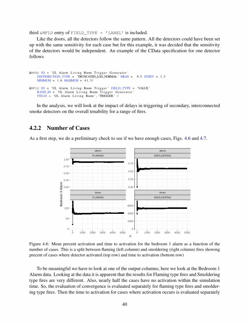
ple 2. . . . . . . . . . . . . . . . . . . . . . . . . . . . . . . . . . . . . . . . . . 394.6 Mean percent activation and time to activation for the bedroom 1 alarm as a func-

tion of the number of cases. This is a split between flaming (left column) andsmoldering (right column) fires showing precent of cases where detector activated(top row) and time to activation (bottom row) . . . . . . . . . . . . . . . . . . . 40

4.7 Standard deviation of percent activation and time to activation for the bedroom1 alarm as a function of the number of cases. This is a split between flaming(left column) and smoldering (right column) fires showing precent of cases wheredetector activated (top row) and time to activation (bottom row) . . . . . . . . . . 41

4.8 Decision tree separating cases where the bedroom alarm sounded from thosewhere it did not. . . . . . . . . . . . . . . . . . . . . . . . . . . . . . . . . . . . 43

4.9 Kernel Density estimate of the time savings for interconnected alarms by fire type. 434.10 Quantiles of the time savings as a function of the number of cases. . . . . . . . . . 444.11 Sample CFAST visualization of a single story commercial structure used for ex-

ample 3. . . . . . . . . . . . . . . . . . . . . . . . . . . . . . . . . . . . . . . . 464.12 Sample HRR inputs for fires in a single story commercial structure used for ex-

ample 3. . . . . . . . . . . . . . . . . . . . . . . . . . . . . . . . . . . . . . . . 474.13 Convergence by the number of runs. . . . . . . . . . . . . . . . . . . . . . . . . . 49

xi

List of Tables

1.1 CFAST Inputs That Can be Varied Based on User-Defined Distributions . . . . . . 41.2 CFAST Fire Inputs That Can be Varied Based on User-Defined Distributions . . . 81.3 CFAST Fire Time Histories That Can be Varied Based on One or More User-

Defined Distributions . . . . . . . . . . . . . . . . . . . . . . . . . . . . . . . . 8

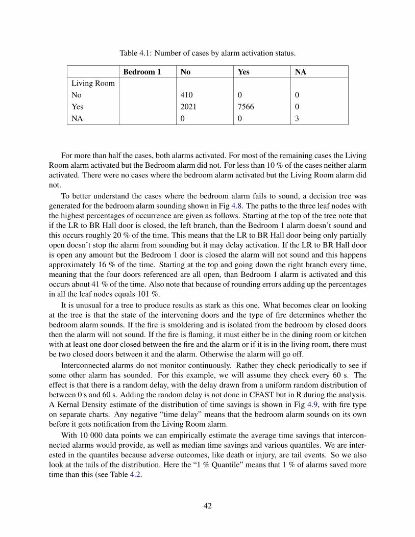
4.1 Number of cases by alarm activation status. . . . . . . . . . . . . . . . . . . . . . 424.2 Quantiles of delay time for bedroom alarm activation . . . . . . . . . . . . . . . . 444.3 Selected result for sensitivity of maximum heat FED. . . . . . . . . . . . . . . . . 504.4 Selected results for sensitivity of time to non-viability for Foyer Heat FED. . . . . 51

B.1 CFAST Input File Keywords . . . . . . . . . . . . . . . . . . . . . . . . . . . . . 64B.2 Monte Carlo Header Parameters (MHDR namelist group) . . . . . . . . . . . . . . 65B.3 Monte Carlo Random Generators (MRND namelist group) . . . . . . . . . . . . . . 66B.4 Monte Carlo Input Field Generators (MFLD namelist group) . . . . . . . . . . . . 67B.5 &MFLD Inputs That Can be Varied Based on User-Defined Distributions . . . . . . 68B.6 Monte Carlo Fire Generators (MFIR namelist group) . . . . . . . . . . . . . . . . 72B.7 Monte Carlo Statistics Plots (MSTT namelist group) . . . . . . . . . . . . . . . . . 75

xii

Chapter 1

Getting Started

The Monte Carlo method is "a broad class of computational algorithms that use repeated randomsampling to obtain numerical results." [2] Stanislaw Ulam is credited with inventing the modernversion of the Markov Chain Monte Carlo method while working on nuclear weapons projectsin the 1940s [3]. Its application in fire safety dates to at least the 1980s with research ongoingto better understand equivalence between the then current standard prescriptive designs and moreperformance-based designs. Bukowski [4] suggested using the Monte Carlo method as a meansof demonstrating when alternative designs were as safe or safer than prescriptive code compliantdesigns. The basic idea was to take a design made to meet code and compare its fire safety per-formance to an alternative design using a set of scenarios with a range of fires appropriate for theoccupancy. If the relative performance of the alternative design was as good or better than the codecompliant design, that would be justification for having the alternative design approved. Clarke etal. [5], as part of demonstrating the viability of using a computer model to predict fire safety, useda Monte Carlo analysis using the Consolidated Fire and Smoke Transport (CFAST) model to pre-dict fire statistics for a residential application. The process continued and now building codes [6]and engineering handbooks [7] provide a legal and technical structure for a fire performance-basedanalysis using, in part, Monte Carlo methods to characterize the relative fire hazard performanceof designs.

Work continued to better characterize the Monte Carlo method in its use in fire safety researchand design. Notarianni [8] used Monte Carlo methods to characterize and quantify uncertainty inperformance-based designs for fire safety. Bruns [9], in a study using Monte Carlo methods toassess the impact of inner liners in residential upholstered furniture, formalized the mathematicsfor applying the Monte Carlo method to fire hazard analysis as a means to further incorporate themethod in regular performance-based designs.

Monte Carlo methods and systematic variation of modeling variables are already used in thefire protection industry. The US nuclear power industry makes use of Monte Carlo and othermethods with large numbers of model runs to generate statistics to quantify risk. Some examplesinclude NUREG/CR-6850 Volume 2 Appendix L [10], NUREG-2178 Volume 1 [11] Chapter 5,obstructed plumes, NUREG-2178 Volume 2 [12] Chapter2 2 and 3, obstructed radiation, Chapter5, Motors and transformers, Chapter 6, wall and corner effects, and chapter 7, main control boards.

At one time issues of both insufficient computational power and a lack of tools designed to dothe analysis were obstacles to using Monte Carlo methods. However, it is now relatively easy toobtain the computational power and storage to generate and analyze huge amounts of data. What

1

is still largely lacking are the tools to make the process tenable. To that end, the Fire ResearchDivision at the National Institute of Standards and Technology (NIST) has been exploring theprocess [13, 14, 15, 16] in order to develop tools that will make Monte Carlo fire hazard analysisa more widely used form of analysis using the Consolidated Fire And Smoke Transport (CFAST)model. The result of this effort is the CFAST Fire Data Generator (CData), documented in thisreport.

The fire model being used, CFAST, is documented by four publications, a user’s guide [17], atechnical reference guide [18] a verification and validation guide [19], and a configuration man-agement guide [20]. The user’s guide describes how to use the model and the input editor CEdit.The technical reference guide describes the underlying physical principles, provides a compar-ison with other models, and includes an evaluation of the model following the guidelines ofASTM E1355 [1]. The model verification and validation guide documents verification and val-idation efforts for the model. The configuration management guide documents the processes usedduring the development and validation of the model. This guide is a companion to the CFAST soft-ware and describes the use of the program CData to generate, summarize, and analyze numerousCFAST simulations.

1.1 InstallationThe CFAST distribution consists of a self-extracting set-up program for Windows-based personalcomputers. After downloading the set-up program, double-clicking on the file’s icon walks youthrough a series of steps for installation of the program. The most important part of the installa-tion is the creation of a folder (C:\Program Files\CFAST by default) in which the CFAST exe-cutable files and supplemental data files are installed. Sample input files are found in the Examplesfolder. CData is installed as part of the CFAST distribution.

CData also makes use of the statistical software, R, for selected analyses of the data generatedfor multiple CFAST runs. R can be downloaded from https://www.r-project.org/.

1.2 Defining the Question and the AnalysisAs briefly discussed in the introduction significant research has gone into understanding the basicrequirements for a Monte Carlo analysis in a fire safety analysis [4, 5, 6, 7, 9]. Several key areasthat need to be addressed in the analysis include definition of:

1. Community / Building / Occupant characteristics

2. Fire scenarios

3. Analysis variables / Criteria for comparisons

4. Statistical analysis of calculation results

Community, building, and fire characteristics define the physical geometries of the model sim-ulations (the range of building geometries, vents between different compartments and compart-ments to the outside, and the range and position of fires to be studied). Occupant characteristics

2

https://www.r-project.org/

and criteria for comparisons define additional model inputs that may be necessary for analysis ofcalculation results (fire detection devices, the choice of additional model outputs to characterizetenability along egress paths, fire severity, or building structural integrity, for example). For themost part, community and occupant characteristics are outside the scope of this report which fo-cuses on developing the range of CFAST model inputs needed to run the desired set of simulations.These may be defined by a single deterministic set of inputs (a single building geometry or desiredfire for study), a collection of different, specific inputs (such as a set of specific building designsof interest), or a statistically-determined range of inputs (for example, defining ranges of com-partment sizes or smoke detector activation from experimentally-determined distributions). Thissection details the process for defining a series of input files for analysis with examples for eachmajor step in the process.

1.2.1 Building CharacteristicsIn CFAST, compartment geometry includes definition of the number of compartments, their size(length, width, and height), and their placement in relation to other compartments. In the studyof a single structure, this is simply an enumeration of each compartment. Figure 1.1 shows thecompartments in a single structure in a CFAST simulation.

Figure 1.1: Sample CFAST visualization of a single structure subject to a fire.

Of course, if it is desired to study the impact of fires in a set of more than one specific building,the compartment geometry and placement could be defined by multiple individual buildings withthe specific building chosen for an individual scenario chosen at random or from a distributionrepresenting the population of each building type in the community under study.

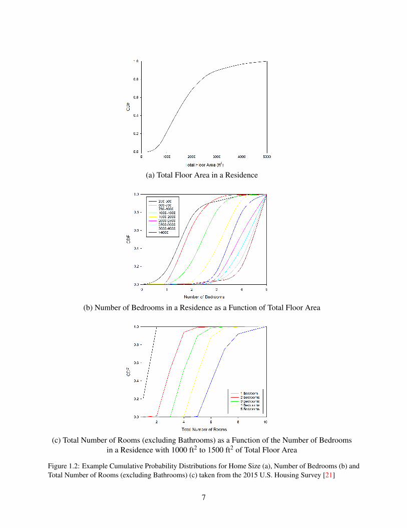
The set of buildings for study can also be chosen from distributions of building and roomcharacteristics. For example Figure 1.2 shows the distribution of the total floor area in a residence,the number of bedrooms in a residence depending on the total floor area, the total number of roomsgiven a certain number of bedrooms (here shown for residences from 1000 ft2 to 1500 ft2)1, alltaken from the 2015 U.S. Housing Survey [21]. Creating a compartment geometry from these datacan be thought of as a six step process:

1NIST uses SI units but in this case English units are used to be consistent with the units used in the U.S. HousingSurvey

3

1. randomly select the total floor area of the structure, Fig. 1.2(a);

2. randomly select the total number of bedrooms for a structure of the size chosen in step 1, Fig.1.2(b);

3. randomly select the total number of rooms in the structure of the chosen size and number ofbedrooms (Fig. 1.2(c) shows a sample distribution for homes ranging from 1000 ft2 to 1500 ft2.Distributions for other home sizes are available in ref. [21]);

4. determine room sizes based on a distribution of bedroom sizes, allocating left over space to theother rooms;

5. connect compartments as desired (for example by randomly setting vents as open or closedbetween compartment pairs); and

6. ensure that the resulting structure is realizable (This random approach to generating connec-tions has a probability of resulting in a floorplan that cannot be instantiated in a single story.More technically, if the floorplan is thought of as a graph with the rooms as vertices and theconnections as edges, some of the randomly generated graphs will be nonplanar for cases withmore than four rooms. A planar graph is one that can be drawn on a piece of paper and none ofthe edges cross. The probability of generating a nonplanar floorplan increases as the number ofrooms increases. In order to eliminate such nonphysical cases from the analysis, any randomlygenerated floorplan can be checked for planarity and rejected if necessary and replaced by anew randomly generated floorplan).

Other characteristics of the structure such as materials of construction, vent openings, firedefinitions, measurement targets, sprinklers, and detection devices can be varied as desired for theproblem being studied. Table B.5 shows variables in the modeling that can be varied based onuser-defined distributions 2.

Table 1.1: CFAST Inputs That Can be Varied Based on User-Defined Distributions

Category Input UnitsAmbient Conditions Interior Temperature ◦C

Exterior Temperature ◦CRelative Humidity %

Thermal Properties Thermal Conductivity kW/(m ◦C)Specific Heat kJ/(kg ◦C)Density kg/m3

Default Thickness mEmissivity

Compartments Width mDepth mHeight mWall Leak Area Ratio m2/m2

2The content of this table follows the form of that used in B-Risk [22], adapted to be applicable to the calculationalcapabilities of the CFAST model.

4

Table 1.1: Continued

Category Input UnitsFloor Leak Area Ratio m2/m2

Compartment MaterialsWall Vents Sill m

Soffit mWidth mOpen/Close Times sOpen/Close Fractions 0-1Initial Opening Fraction 0-1Open/Close Time sFinal Opening Fraction 0-1Setpoint s, ◦C, or kW/m2

Pre-Activation Fraction 0-1Post-Activation Fraction 0-1

Ceiling / Floor Vents Cross-Sectional Area m2

Open/Close Times sOpen/Close Fractions 0-1Initial Opening Fraction 0-1Open/Close Time sFinal Opening Fraction 0-1Setpoint s, ◦C, or kW/m2

Pre-Activation Fraction 0-1Post-Activation Fraction 0-1

Mechanical Vents From Compartment Area m2

From Compartment Height mTo Compartment Area m2

To Compartment Height mFlow Rate m3/sBegin Dropoff PaEnd Dropoff PaOpen/Close Times sOpen/Close Fractions 0-1Initial Opening Fraction 0-1Open/Close Time sFinal Opening Fraction 0-1Setpoint s, ◦C, or kW/m2

Pre-Activation Fraction 0-1Post-Activation Fraction 0-1Filter Efficiency %Begin Filtering Time s

Fires See Section 1.2.2Targets Width Target Position m

Depth Target Position m

5

Table 1.1: Continued

Category Input UnitsHeight Target Position mWidth Normal Vector 0-1Depth Normal Vector 0-1Height Normal Vector 0-1Target Points To Selection ListThickness mInternal Temperature Location m

Detection / Suppression Width Position mDepth Position mHeight Position mActivation Temperature ◦CActivation Obscuration %/mRTI (m s)1/2

Spray Density m/s

6

(a) Total Floor Area in a Residence

(b) Number of Bedrooms in a Residence as a Function of Total Floor Area

(c) Total Number of Rooms (excluding Bathrooms) as a Function of the Number of Bedroomsin a Residence with 1000 ft2 to 1500 ft2 of Total Floor Area

Figure 1.2: Example Cumulative Probability Distributions for Home Size (a), Number of Bedrooms (b) andTotal Number of Rooms (excluding Bathrooms) (c) taken from the 2015 U.S. Housing Survey [21]

7

1.2.2 Fire ScenariosIndividual Variables

The quantitative definition of fires is arguably the most important [23] and complex of all the inputsin any fire modeling scenario. It includes specification of the fire location, fuel composition, andignition criterion. Heat release rate, burning area, and species yields, which can vary with timeover the course of the fire are covered in the next section.

Table 1.2: CFAST Fire Inputs That Can be Varied Based on User-Defined Distributions

Category Input UnitsFire Location Compartment Selection List

Width Position mDepth Position m

Fuel Composition Carbon Molecules ≥ 0Hydrogen Molecules ≥ 0Oxygen Molecules ≥ 0Nitrogen Molecules ≥ 0Chlorine Molecules ≥ 0Heat of Combustion kJ/kgRadiative Fraction 0 - 1

Ignition Criteria Ignition Criterion Selection ListSetpoint s, ◦C, or kW/m2

Time Histories See Table 1.3

Time Histories

Key to the fire definition are the time histories of heat release rate, burning area, and species yieldsof important combustion products. In some scenarios, these may be constants, but in others, theycan vary with time.

Table 1.3: CFAST Fire Time Histories That Can be Varied Based on One or More User-DefinedDistributions

Category Input UnitsTime Histories Time s

HRR kWFire Height mFire Area m2, >0CO Yield kg CO/kg fuelSoot Yield kg Soot/kg fuelHCN Yield kg HCN/kg fuel

8

Chapter 2

Defining Data for Analysis, CData Inputs

This chapter describes the inputs that are used to define a set of scenarios for analysis. The inputsallow the user to define one or more distributions that are then used to vary individual variableswithin a CFAST input file. Each subsection will discuss one set of namelist inputs and what eachof the parameters does. All the inputs are combined in Appendix B to serve as a reference forcommands. Examples are included in with each section to

Section 3.1 has additional details on how to run CData. One example of running CData from acommand line is the following

cdata Simple.in -P

In this case the base file name of the CData/CFAST input file, Simple, is referred to as the<project> and that name is used as part of the name of a number of different files for the seriesof calculations.

2.1 Namelist MHDRThe &MHDR inputs specify general inputs of the scenarios to be generated including the total numberof cases to be generated, seeds for the random number generator, and locations for input and outputfiles.

NUMBER_OF_CASES (default value 1): specifies the number of cases that the preprocessorwill generate.

SEEDS (default value, software chosen random integer pair): defines an integer pair used to de-termine random number seeds for distributions. Any two integers (excluding -1001 which isused internally to indicate default values) may be specified. Including random seeds here willensure that the same cases will be generated each time the preprocessor is run for a given inputfile. Changing the random seeds (or other inputs) will result in a different set of input files.All seeds are written in the <project>_seeds.csv file, if specified. Note that if you do notinclude SEEDS in the input file everytime the file is run a different set of cases will be created.

WRITE_SEEDS (default value, .TRUE.): if .TRUE., all random number seeds are saved in thefile <project>_seeds.csv.

9

PARAMETER_FILE (default value, <project>_parameters.csv: Summary output file fromthe preprocessor that list the CFAST file names and parameter values for inputs varied for eachCFAST scenario in the set of generated CFAST cases. This file is combined with the summarystatistics generated by the accumulator module.

WORK_FOLDER (default value, current folder): folder where the preprocessor creates its set ofCFAST inputs file and where the accumulator looks for CFAST output files to be processed.

OUTPUT_FOLDER (default value, current folder): folder where the accumulator or statisticsmodules put their output files of analysis results.

Examples:

&MHDR NUMBER_OF_CASES = 10000 /&MHDR NUMBER_OF_CASES = 20000 WRITE_SEEDS = .TRUE .

PARAMETER_FILE = ' P a r a m e t e r F i l e ' OUTPUT_FOLDER = ' . . \ p r o j e c t ' /

2.2 Namelist MRNDThe &MRND input defines a random number generator that uses a number of inputs to specifydistributions for variation. A generator specifies a single random variable for each case so thatevery input using a particular generator will get the same value for each case. &MRND alwaysreturns a real value. In the simplest cases every field that a user wants to vary will require aseparate random generator. However, if the desire is to have all the rooms have the same heightceiling, then all the fields can use the same random number generator.

ID Distributions are defined by a unique alphanumeric name. This may be as simple as a singlecharacter or number, or a description of the distribution. All IDs must be unique throughout aninput file. The ID can be any ASCII string up to 128 characters.

FYI A user defined comment that can provide additional information about the input.

DISTRIBUTION_TYPE identifies the type of distribution. Additional required inputs depend ofthe type of distribution defined. Allowed distributions are

CONSTANT requires additional inputs CONSTANT. Returns a real number with a value ofCONSTANT.

LINEAR requires additional inputs MINIMUM and MAXIMUM. Returns real values from theMINIMUM value to MAXIMUM incremented by 1/NUMBER_OF_CASES.

UNIFORM requires additional inputs MINIMUM and MAXIMUM. Returns real values.

TRIANGLE requires additional inputs MINIMUM, MAXIMUM, and PEAK. Returns real values.

NORMAL requires additional inputs MEAN and STDEV. Returns real values.

10

TRUNCATED_NORMAL requires additional inputs MEAN and STDEV, and also MINIMUM,and MAXIMUM. The NORMAL distribution type returns values from −∞ to +∞. TheTRUNCATED_NORMAL distribution type allows the user to limit the values returned to aspecified range. Returns real values.

LOG_NORMAL requires additional inputs MEAN and STDEV. Returns real values.

TRUNCATED_LOG_NORMAL MEAN and STDEV, MINIMUM, and MAXIMUM. TheLOG_NORMAL distribution type returns values from −∞ to +∞. TheTRUNCATED_LOG_NORMAL distribution type allows the user to limit the values returnedto a specified range. Returns real values.

BETA requires additional inputs ALPHA, BETA, MINIMUM, and MAXIMUM. Returns real values.

GAMMA requires additional inputs ALPHA and BETA. Returns real values.

TRUNCATED_GAMMA requires additional inputs ALPHA, BETA, MINIMUM, and MAXIMUM.The GAMMA distribution type returns values from 0 to +∞. TheTRUNCATED_GAMMA distribution type allows the user to limit the values returned to aspecified range. Returns real values.

USER_DEFINED_CONTINUOUS requires additional inputs PROBABILITIES, and VALUES.The number of PROBABILITIES inputs must be one less than then number of VALUESinputs. Returns real values. Endpoints of each interval are inclusive and interior pointsare continuous. For example, if you have VALUES = 1.,3.,8. and PROBABILITIES =0.3,0.7, there’s then a 30% probability of getting a real number between 1.0 and 3.0 anda 70% probability of getting a real number between 3.0 and 8.0.

USER_DEFINED_DISCRETE requires additional inputs PROBABILITIES, and VALUES.The number of PROBABILITIES inputs must match the number ofVALUES inputs. Returns real values.

RANDOM_SEEDS like RANDOM_SEEDS in &MHDR, an integer pair specifies initial seeds for therandom number generator, but applies only to the specific distribution. Any two integers (ex-cluding -1001 which is used internally to indicate default values) may be specified. Providinga specific pair of integer values ensures the distribution returns the same set of integers eachtime cases are created from the input file. By default (i.e., not including this input) will resultsin a different set of integer values for this distribution each time cases are created. All seedsare written in the <project>_seeds.csv file, if specified.

CONSTANT is a single real value. It is the value that is returned by the CONSTANT distribution.

VALUES a set of real numbers for the USER_DEFINED_... distribution types. Inputs are inputas real constants. Values for an individual scenario are chosen randomly from the list of valuesprovided.

PROBABILITIES a set of probabilities values for the USER_DEFINED.̇. distribution types.These are not cumulative probabilities and the total of all values must add to 1.0

MINIMUM minimum value for the UNIFORM, TRIANGLE, TRUNCATED_NORMAL,TRUNCATED_LOG_NORMAL, TRUNCATED_GAMMA, and LINEAR distribution types.

11

MAXIMUM maximum value for the UNIFORM, TRIANGLE, TRUNCATED_NORMAL,TRUNCATED_LOG_NORMAL, TRUNCATED_GAMMA, and LINEAR distribution types.

PEAK peak value for the TRIANGLE distribution type.

ALPHA alpha value for the BETA and GAMMA distribution types.

BETA beta value for the BETA and GAMMA distribution types.

MEAN mean value for the NORMAL; geometric mean value for the LOG_NORMAL distribution type.

STDEV standard deviation value for the NORMAL; geometric standard deviation value for theLOG_NORMAL distribution type.

MINIMUM_FIELD specifies the ID of the specific &MFLD within the input whose value is tobe taken as the minimum value of the distribution returned. It allows the range to be defined byanother input. For example, if the &MRND input is used to vary the ceiling height the top of a ventcan be used as the lowest value for the ceiling height by including a MINIMUM_FIELD inputwith the ID for the FIELD that sets the vent height input such as MINIMUM_FIELD="Vent1", "TOP" to limit how low the height of the compartment is set.

MAXIMUM_FIELD specifies the ID of the specific &MFLD within the input whose value is tobe taken as the maximum value of the distribution returned. It allows the range to be defined byanother input. For example, if the &MRND input is used to vary the ceiling height the top of a ventcan be used as the lowest value for the ceiling height by including a MAXIMUM_FIELD inputwith the ID for the FIELD that sets the ceiling height input such as MAXIMUM_FIELD="Comp1", "HEIGHT" to limit how high the top of the vent is set.

MINIMUM_OFFSET is a value added to MINIMUM value (or value returned from a MINIMUM_FIELD.It is typically used to bound the value to allowable values in a compartment geometry (for ex-ample, to ensure a vent bottom is above the floor of a compartment).

MAXIMUM_OFFSET is a value added to MAXIMUM value (or value returned from a MAXIMUM_FIELD.It is typically used to bound the value to allowable values in a compartment geometry (for ex-ample, to ensure a vent top is below the ceiling of a compartment).

ADD_FIELD specifies the ID of the specific &MFLD within the input whose value is to be addedto the value generated by the current random generator. Suppose that a vent is to be closed ata random time, then a second random generator can be set as a constant 1 s and have the first&MFLD as the ADD_FIELD to have the time the vent finishes closing to be 1 s after the start.

Example:

&MRND ID = ' Example r and g e n e r a t o r ' , TYPE = 'UNIFORM ' , MINIMUM = 10 , MAXIMUM = 50 /&MRND ID = ' Second rand g e n e r a t o r ' , TYPE = 'NORMAL ' , MEAN = 0 , STDEV = 1 /&MRND ID = ' P r o p e r t y G e n e r a t o r ' DISTRIBUTION_TYPE = ' USER_DEFINED_DISCRETE '

VALUES = 1 , 2 PROBABILITIES = 0 . 5 , 0 . 5 /&MRND ID = ' Flaming I g n i t i o n Peak G e n e r a t o r ' DISTRIBUTION_TYPE = 'TRUNCATED_NORMAL '

MEAN = 23 STDEV = 7 MINIMUM = 1 0 . 0 MAXIMUM = 3 0 . 0 /

12

2.3 Namelist MFLDThe basic structure in CData to change values of a CFAST input file is the &MFLD input. Itsbasic function is to marry a random generator given in a &MRND namelist to a particular value ina CFAST input file. Depending on how many fields are to be changed in a single Monte Carloanalysis there could be a very large number of &MFLD inputs and unlike &MRND inputs, there isa one to one match between &MFLD inputs and CFAST entries to be changed.

ID Varied input fields are defined by a unique alphanumeric name. This may be as simple as asingle character or number, or a description of the field. All IDs must be unique throughout aninput file. The ID can be any ASCII string up to 128 characters.


RAND_ID specifies the ID of associated &MRND input used to provide random inputs for the field.These may be unique to each field input or more than one field input may use the same &MRNDinput to coordinate values for multiple input fields. The number of inputs in the &MRND inputmust match those for the field type.

FIELD specifies the name of the specific input (i.e., the name of a compartment, vent, etc.) and thespecific field within that input that is to be varied. For example, FIELD="Comp 1","HEIGHT"

would vary the height of the compartment named Comp 1.

FIELD_TYPE specifies the type of field data used to fill in values in the specified field. Addi-tional inputs depend on the type of field specified. Allowed field types are VALUE, SCALING,LABEL, and INDEX. VALUE simply takes the value returned from the specified random genera-tor and places it directly in the specified field. SCALING takes the returned value and multipliesby the BASE_SCALING_VALUE and puts that value in the field. INDEX requires the randomgenerator to return integers as an index into the VALUES input (starting at 1 to the number ofinputs in the VALUES input for the current &MFLD input). The value in the INDEX_TYPE, REAL,INTEGER, STRING, or LOGICAL, array at the index is placed in the field.

PARAMETER_COLUMN_LABEL specifies the column title for this input field in the param-eters file, <project>_parameters.csv. If it is not included CData will use a combinationof the FIELD inputs to create a column label.

ADD_TO_PARAMETERS set to .TRUE. to include the value of the field in the parameters file,<project>_parameters.csv. Default value is .TRUE.

VALUE_TYPE defines the input type in the VALUES included in the input. Must be INTEGER,REAL, STRING, or LOGICAL.

REAL_VALUES a set of values for the INDEX field type. Values for an individual scenario arechosen randomly from the list of values provided. The type of the inputs is determined by thetype of value needed from the FIELD input but all inputs in the VALUES inputs are specified ina character array input.

13

INTEGER_VALUES a set of values for the INDEX field type. Values for an individual scenarioare chosen randomly from the list of values provided. The type of the inputs is determined bythe type of value needed from the FIELD input but all inputs in the VALUES inputs are specifiedin a character array input.

STRING_VALUES a set of values for the INDEX field type. Values for an individual scenario arechosen randomly from the list of values provided. The type of the inputs is determined by thetype of value needed from the FIELD input but all inputs in the VALUES inputs are specified ina character array input.

LOGICAL_VALUES a set of values for the INDEX field type. Values for an individual scenarioare chosen randomly from the list of values provided. The type of the inputs is determined bythe type of value needed from the FIELD input but all inputs in the VALUES inputs are specifiedin a character array input.

SCENARIO_TITLES an optional set of character strings that describe each of the different fieldsin an INDEX set of values.

BASE_SCALING_VALUE Initial value of the field for the SCALING type field. Defaults to thevalue in the base input file if not included.

Examples:The following example shows the height of the bedroom varying uniformly from 2.44 m to

3.66 m.

&MRND ID = ' Room h e i g h t g e n e r a t o r ' , TYPE = 'UNIFORM ' , MINIMUM = 2 . 4 4 , MAXIMUM = 3 . 6 6 /&MFLD ID = ' H e ig h t bedroom ' FIELD = ' Bedroom ' , 'HEIGHT ' RAND_ID = ' Room h e i g h t g e n e r a t o r '

PARAMETER_COLUMN_LABEL = ' Bedroom h e i g h t ' /

The following example shows the height of a door to the bedroom in the above example varyingfrom a minimum of 2 m to a maximum 0.15 m below the ceiling of the varying height of thebedroom ceiling.

&MRND ID = ' Door Top G e n e r a t o r ' DISTRIBUTION_TYPE = 'UNIFORM ' VALUE_TYPE = 'REAL 'MINIMUM = 2 . 0 MAXIMUM_FIELD = ' He igh t bedroom ' MAXIMUM_OFFSET = −0.15 /

&MFLD ID = ' Door Top ' FIELD_TYPE = 'VALUE ' RAND_ID = ' Door Top G e n e r a t o r 'FIELD = ' Wall Vent ' 'TOP ' /

The next example is of both FIELD_TYPE = INDEX and FIELD_TYPE = LABEL. A doorhas 5 postions, fully open, three quaters open, half open, one quater open, and closed. The closeposition is represented with the vent having the full width but the top of the vent only being 2.5 cmabove the floor. The other four positions are determined by the width of the door with the top atfull height. Because two parameters are being coordinated and more could be included a LABELcolumn is included to provide a single place to determine the state of the door. For more about thisexample look at section 4.2

&MRND ID = ' G e n e r a t o r f o r DR LR 1 ' DISTRIBUTION_TYPE = ' USER_DEFINED_DISCRETE 'VALUES = 1 , 2 , 3 , 4 , 5 PROBABILITIES = 0 . 2 , 0 . 2 , 0 . 2 , 0 . 2 0 . 2 /

14

&MFLD ID = ' H e ig h t DR LR 1 ' FIELD_TYPE = ' INDEX 'RAND_ID = ' G e n e r a t o r f o r DR LR 1 ' REAL_VALUES = 2 . 4 , 2 . 4 , 2 . 4 , 2 . 4 0 .025FIELD = 'DR LR 1 ' , 'TOP ' ADD_TO_PARAMETERS = .TRUE . /

&MFLD ID = ' Width DR LR 1 ' FIELD_TYPE = ' INDEX 'RAND_ID = ' G e n e r a t o r f o r DR LR 1 ' REAL_VALUES = 0 . 9 6 0 . 7 2 0 . 4 8 0 . 2 4 0 . 9 6FIELD = 'DR LR 1 ' , 'WIDTH ' ADD_TO_PARAMETERS = .TRUE . /

&MFLD ID = ' Labe l DR LR 1 ' FIELD_TYPE = 'LABEL 'RAND_ID = ' G e n e r a t o r f o r DR LR 1 'STRING_VALUES = ' open ' ' t h r e e − f o u r t h ' ' one − h a l f ' ' one − f o u r t h ' ' c l o s e d 'ADD_TO_PARAMETERS = .TRUE .PARAMETER_COLUMN_LABEL = 'DR LR 1 Opening S t a t u s ' /

The last example is for FIELD_TYPE = SCALING. Section 4.3 is a sensitivity analysis. In it anumber of compartments are connected in such a way that their hieghts need to be the same. Theexample shows how three of the compartments are set to scale the their heights together.

&MRND ID = ' S c a l i n g h e i g h t ' ,FYI = ' S c a l i n g f o r e v e r y t h i n g t h a t has t h e same max h e i g h t ' ,DISTRIBUTION_TYPE = 'UNIFORM ' , MINIMUM = 0 . 9 MAXIMUM = 1 . 1 /

&MFLD ID = ' F o r y e r h e i g h t ' FIELD_TYPE = 'SCALING ' FIELD = ' Foyer ' 'HEIGHT 'RAND_ID = ' S c a l i n g h e i g h t ' ADD_TO_PARAMETERS = .TRUE .PARAMETER_COLUMN_LABEL = ' F o y e r _ a n d _ H a l l s _ h e i g h t ' /

&MFLD ID = ' Even Hal lway h e i g h t ' FIELD_TYPE = 'SCALING ' FIELD = ' Even Hallway ' 'HEIGHT ' RAND_ID= ' S c a l i n g h e i g h t ' /

&MFLD ID = ' Odd Hallway h e i g h t ' FIELD_TYPE = 'SCALING ' FIELD = ' Odd Hallway ' 'HEIGHT ' RAND_ID =' S c a l i n g h e i g h t ' /

15

2.4 Namelist MFIRAutomatically-generated fires are created for an individual test case by modifying an existing fireinput in the input file. The &MFIR input allows the user to either scale the HRR curve (multiplyingthe time and/or HRR values by a constant defined by a user-specified distribution), to define apower law fire based on several inputs, or to modify individual time points from a constant definedby a user-specified distribution.

ID All inputs are defined by a unique alphanumeric name. This may be as simple as a singlecharacter or number, or a description of the field. All IDs must be unique throughout an inputfile. The ID can be any ASCII string up to 128 characters.


FIRE_ID Specifies the associated fire in the data file that is used as a template to be modified bythis &MFIR input. All inputs in the current &MFIR namelist will modify this fire.

MODIFY_FIRE_AREA_TO_MATCH_HRR IF set to .TRUE., the fire area is calculated fromthe heat release rate values for the time curve from the formula. Values are calculated fromheat release rate such that the fire Froude number is unity1.

FIRE_COMPARTMENT_RANDOM_GENERATOR_ID A random generator that returns anindex to pick the compartment the fire is located. Usually usesUSER_DEFINED_DISCRETE_DISTRIBUTION.

FIRE_COMPARTMENT_IDS A list of compartment names that have a chance of having thefire in them. This matches the index chosen by FIRE_COMPARTMENT_RANDOM_GENERATOR_IDto actual compartment names in the input file.

ADD_FIRE_COMPARTMENT_ID_TO_PARAMETERS set to .TRUE. to include the valueof the field in the parameters file, <project>_parameters.csv. Default value is .TRUE.

FIRE_COMPARTMENT_ID_COLUMN_LABEL specifies the column title for this input fieldin the parameters file, <project>_parameters.csv. If it is not included, it will be filled inby the code.

Fires can be defined by either scaling time and/or HRR values from a base fire or by defininga power law fire growth / decay with a peak plateau period. Either fire can be proceeded byan optional period of incipient fire growth period. Firstly, the inputs for the incipient fire aredescribed.

FLAMING_SMOLDERING_INCIPIENT_RANDOM_GENERATOR_ID This and the twoentries INCIPIENT_FIRE_TYPES and TYPE_OF_INCIPIENT_GROWTH work together. Thisrandom generator, if included, switches the incipient fire between flaming and smoldering.This is an INDEX field type. The types being switched through are listed inINCIPIENT_FIRE_TYPES. TYPE_OF_INCIPIENT_GROWTH has to be set to RANDOM.

1The Fire Froude Number, Q̇∗, is defined as Q̇∗ = Q̇ρ∞cpT∞

√gDD2 . It is essentially the ratio of the fuel gas exit

velocity and the buoyancy-induced plume velocity. Jet fires are characterized by large Froude numbers. Typicalaccidental fires have a Froude number near unity.

16

INCIPIENT_FIRE_TYPES A list made up of ’FLAMING’ and ’SMOLDERING’. This allowsusers to coordinate the incipient beginning of the fire with other inputs in the scenario.

TYPE_OF_INCIPIENT_GROWTH Defaults to NONE but can be FLAMING, SMOLDERING, andRANDOM

FLAMING_INCIPIENT_DELAY_RANDOM_GENERATOR_ID This is the first of the flam-ing set of generators and defines an associated &MRND ID that defines the length of the incipientflaming fire burning period. If you do not want the value to change you can set it up to aCONSTANT random generator. If included, bothFLAMING_IGNITION_DELAY_RANDOM_GENERATOR_ID andPEAK_FLAMING_IGNITION_RANDOM_GENERATOR_ID must be defined.

FLAMING_INCIPIENT_PEAK_RANDOM_GENERATOR_ID This is the second of the flam-ing set of generators and defines an associated &MRND ID that defines the final HRR for theincipient flaming fire ramp. If you do not want the value to change you can set it up to aCONSTANT random generator. If included, bothFLAMING_IGNITION_DELAY_RANDOM_GENERATOR_ID andPEAK_FLAMING_IGNITION_RANDOM_GENERATOR_ID must be defined. This one determinesthe final HRR for the flaming fire ramp. It is important to understand that using this means thefirst two HRR points will be overwritten and all times for all entries in the fire will be set to thesame.

SMOLDERING_INCIPIENT_DELAY_RANDOM_GENERATOR_ID This is the smolder-ing pair that match the above.

SMOLDERING_INCIPIENT_PEAK_RANDOM_GENERATOR_ID Same as above for smol-dering fire.

ADD_INCIPIENT_TYPE_TO_PARAMETERS set to .TRUE. to include a label of the type ofincipient fire in the parameters file, <project>_parameters.csv. Default value is .TRUE.Column displays ’FLAMING’ or ’SMOLDERING’ depending on which type of incipient firein the case.

INCIPIENT_TYPE_COLUMN_LABEL specifies the column title for this input field in theparameters file, <project>_parameters.csv. If it is not included andADD_INCIPIENT_TYPE_TO_PARAMETERS is .TRUE. the column label will be filled in byCData with <FIRE_ID>_INCIPIENT_FIRE_TYPE.

Secondly, inputs for the scaling fire are described.

BASE_FIRE_ID For scaling fires only. This provides internal temporary storage for all the basevalues for a fire to be scaled. Typically, it will just be a copy of the corresponding FIRE_ID

input.

SCALING_FIRE_HRR_RANDOM_GENERATOR_ID an associated &MRND ID that definesthe scaling factor that is applied to all the HRR values in a fire. This is done before the incipientfire model is calculated so it won’t impact the delay or HRR value for the incipient fire portionof the fire curve.

17

SCALING_FIRE_TIME_RANDOM_GENERATOR_ID an associated &MRND ID that definesthe scaling value that is applied to all the TIME values in a fire. This is done before the Incipientfire model is calculated so it won’t impact the delay or HRR value for the incipient portion ofthe fire curve.

ADD_HRR_SCALE_TO_PARAMETERS set to .TRUE. to include the value of the field in theparameters file, <project>_parameters.csv. Default value is .TRUE.

HRR_SCALE_COLUMN_LABEL specifies the column title for this input field in the parame-ters file, <project>_parameters.csv. If it is not included, it will be filled in by the code.

ADD_TIME_SCALE_TO_PARAMETERS set to .TRUE. to include the value of the field inthe parameters file, <project>_parameters.csv. Default value is .TRUE.

TIME_SCALE_COLUMN_LABEL specifies the column title for this input field in the param-eters file, <project>_parameters.csv. If it is not included, it will be filled in by the code.

Finally, the inputs for a general power law fire are described. The calculation of the growth anddecay points is straightforward enough. The inputs are t0, t1, Q̇0, Q̇1, and the exponential growthr. The variables t0 and t1 are the beginning and ending time points and Q̇0 and Q̇1 are the HRR atthe beginning and end and r is already defined. For growth t̂ = t + t0 where 0 < t < t1− t0 and fordecay t̂ = t1− t where 0 < t < t1− t0. The equation for the HRR at time t in the growth phase isQ̇(t̂) = ((Q̇1− Q̇0)/(t1− t0)r)t̂ + Q̇0 and for decay is Q̇(t̂) = ((Q̇0− Q̇1)/(t1− t0)r)t̂ + Q̇1. It canbe done based on which, Q̇0 or Q̇1, are larger.

FIRE_TIME_GENERATOR_IDS a set of up to 100 associated &MRND inputs that define thetime intervals for fire growth If you do not want the values to change you can set any of the&MRND inputs to a CONSTANT random generator. The first point is always at t = 0 and Q̇ = 0.If there is an incipient fire defined, that is point two. If there is a power law growth defined(by GROWTH_EXPONENT and GROWTH_EXPONENT, these follow the first or second time point(depending on whether there is an incipient fire defined). If a power law decay is defined(by DECAY_EXPONENT and DECAY_EXPONENT, these are defined by the next to last and lastgenerators defined.

FIRE_HRR_GENERATOR_IDS a set of up to 100 associated &MRND inputs that define the HRRvalues corresponding with each defined time generator. If you do not want the values to changeyou can set any of the &MRND inputs to a CONSTANT random generator.

NUMBER_OF_GROWTH_POINTS specifies the number of data points included in the growthphase of the fire.

NUMBER_OF_DECAY_POINTS specifies the number of data points included in the decayphase of the fire.

GROWTH_EXPONENT specifies the exponent of the power law for the growth phase of thefire. Must be a positive number.

18

GENERATOR_IS_TIME_TO_1054_KW Is a logical. If .TRUE. then the first generator returnsthe time the fires growth will reach 1054 KW and the HRR is determined by combining thisvalue with the corresponding value in the FIRE_TIME_GENERATORS list.

GENERATOR_IS_TIME_TO_PEAK Is a logical and defaults to .TRUE.. If .TRUE., the firstgenerator in the FIRE_HRR_GENERATORS list returns the HRR for that point.

DECAY_EXPONENT specifies the exponent of the power law for the decay phase of the fire.Must be a positive number. Only one of DECAY_EXPONENT or TIME_TO_0_KW can be includedin an &MFIR input.

ADD_HRR_TO_PARAMETERS set to .TRUE. to include the value of the field in the parame-ters file, <project>_parameters.csv. Default value is .TRUE.

ADD_TIME_TO_PARAMETERS set to .TRUE. to include the value of the field in the param-eters file, <project>_parameters.csv. Default value is .TRUE.

TIME_COLUMN_LABELS specifies the column titles for this input field in the parameters file,<project>_parameters.csv. The labels are input as an array of names that can be lessthan or equal to the total number of FIRE_TIME_GENERATORS or FIRE_HRR_GENERATORS.If it is not included or set to NULL, it will be filled in by the code.

HRR_COLUMN_LABELS specifies the column titles for this input field in the parameters file,<project>_parameters.csv. The labels are input as an array of names that can be less thanor equal to the total number of FIRE_TIME_GENERATORS or FIRE_HRR_GENERATORS.If it isnot included or set to NULL, it will be filled in by the code.

Examples:The following example shows a fire that varies± 10 % from a base fire defined in the input file.

Note that the base fire definition is not shown in the example. See the sensitivity analysis examplein section 4.3 for details of the complete fire definition.

&MRND ID = ' S c a l i n g HRR ' , DISTRIBUTION_TYPE = 'UNIFORM ' , MINIMUM = 0 . 9 MAXIMUM = 1 . 1 /&MRND ID = ' S c a l i n g Time ' , DISTRIBUTION_TYPE = 'UNIFORM ' , MINIMUM = 0 . 9 MAXIMUM = 1 . 1 /&MFIR ID = ' S c a l e f i r e ' FIRE_ID = ' F i r e ' BASE_FIRE_ID = ' Base F i r e '

SCALING_FIRE_HRR_RANDOM_GENERATOR_ID = ' S c a l i n g HRR 'SCALING_FIRE_TIME_RANDOM_GENERATOR_ID = ' S c a l i n g Time ' /

The following example shows a fire with a peak HRR ranging from 500 kW to 3000 kW thatgrows linearly to the peak in 10 s, stays at the peak value for 900 s and decays linearly back to0 kW in 10 s.

&MRND ID = ' Peak HRR ' , DISTRIBUTION_TYPE = 'UNIFORM ' MINIMUM = 500 MAXIMUM = 3000 /&MRND ID = ' End of F i r e HRR ' DISTRIBUTION_TYPE = 'CONSTANT ' CONSTANT = 0 /&MRND ID = ' Peak HRR Time I n t e r v a l ' DISTRIBUTION_TYPE = 'CONSTANT ' CONSTANT = 900 /&MRND ID = ' F i r e Time I n t e r v a l ' DISTRIBUTION_TYPE = 'CONSTANT ' CONSTANT = 10 /

&MFIR ID = ' F i r e _ g e n e r a t o r ' FIRE_ID = ' F i r e 'FIRE_TIME_GENERATORS = ' F i r e Time I n t e r v a l ' ' Peak HRR Time I n t e r v a l ' ' F i r e Time I n t e r v a l 'FIRE_HRR_GENERATORS = ' Peak HRR ' ' Peak HRR ' ' End of F i r e HRR ' /

19

The following example defines a t-squared growth rate fire with a peak HRR ranging from150 kW to 1600 kW with a time to peak HRR ranging from 75 s to 1000 s. The fire stays at thepeak value for 10 s and decays linearly back to 0 kW in 10 s.

&MRND ID = ' End of Time Growth G e n e r a t o r ' , DISTRIBUTION_TYPE = 'UNIFORM ' \ \MINIMUM = 75 MAXIMUM = 1000 /

&MRND ID = ' Peak HRR G e n e r a t o r ' , DISTRIBUTION_TYPE = 'UNIFORM ' MINIMUM = 150 MAXIMUM = 1600 /&MRND ID = ' P l a t e a u End Time ' DISTRIBUTION_TYPE = 'CONSTANT ' CONSTANT = 10 /&MRND ID = ' F i r e End Time ' DISTRIBUTION_TYPE = 'CONSTANT ' CONSTANT = 10 /&MRND ID = ' End of F i r e HRR ' DISTRIBUTION_TYPE = 'CONSTANT ' CONSTANT = 0 /

&MFIR ID = ' F i r e _ g e n e r a t o r ' FIRE_ID = 'New F i r e 1 'FIRE_TIME_GENERATORS = ' End of Time Growth G e n e r a t o r ' ' P l a t e a u End Time ' ' F i r e End Time 'FIRE_HRR_GENERATORS = ' Peak HRR G e n e r a t o r ' ' Peak HRR G e n e r a t o r ' ' End of F i r e HRR 'NUMBER_OF_GROWTH_POINTS = 20 GROWTH_EXPONENT = 2 /

This final example defines a fire in one of three positions in one of five fire rooms. The firebegins with an incipient flaming ignition growing from 0 kW to from 10 kW (normally distributedwith a mean of 23 kW and a standard deviation of 7 kW) to 30 kW in from 150 s to 1200 s(normally distributed with a mean of 207 kW and a standard deviation of 46 kW). The ignitionperiod is followed by a t-squared growth to a peak of 130 kW to 4620 kW with a time to 1054 kWof 50 s to 330 s. The fire stays at the peak value for 10 s and decays linearly back to 0 kW in 10 s.

! ! Th i s d e t e r m i n e s t h e f i r e p o s i t i o n , ( 2 , 2 ) , ( 0 , 2 ) ( 0 , − 0 . 0 0 1 ) .! ! The l a s t one i s 1 mm from back w a l l&MRND ID = ' F i r e P o s i t i o n G e n e r a t o r ' DISTRIBUTION_TYPE = ' USER_DEFINED_DISCRETE '

VALUES = 1 2 3 PROBABILITIES = 0 .3333 0 .3333 0 . 3 3 3 4 /&MFLD ID = ' Random x−pos ' FIELD_TYPE = ' INDEX ' RAND_ID = ' F i r e P o s i t i o n G e n e r a t o r '

FIELD = ' Random ' ' X_POSITION ' REAL_VALUES = 2 . 0 0 . 0 0 . 0ADD_TO_PARAMETERS = .TRUE . /

&MFLD ID = ' Random y−pos ' FIELD_TYPE = ' INDEX ' RAND_ID = ' F i r e P o s i t i o n G e n e r a t o r 'FIELD = ' Random ' ' Y_POSITION ' REAL_VALUES = 2 . 0 2 . 0 −0.001ADD_TO_PARAMETERS = .TRUE . /

! ! Th i s one s e t s t h e f i r e room randomly&MRND ID = ' G e n e r a t o r f o r f i r e rooms ' DISTRIBUTION_TYPE = ' USER_DEFINED_DISCRETE '

VALUES = 1 , 2 , 3 , 4 , 5 , 6 PROBABILITIES = 0 .16666 0 .16666 0 .16666 0 .16666 0 .16666 0 . 1 6 6 7 /

! ! These d e f i n e t h e f i r e HRR c u r v e as a f l a m i n g i g n i t i o n ( growing from 0 kW t o 10 kW − 30 kW! ! i n from 150 s t o 1200 s , bo th as t r u n c a t e d normal d i s t r i b u t i o n s! ! c o n s i s t e n t w i th d a t a from Cleary , T .G. , " Improv ing Smoke Alarm Per fo rmance − J u s t i f i c a t i o n f o r! ! New Smolde r ing and Flaming T e s t C r i t e r i a " , i n T e c h n i c a l Note 1837 .! ! 2014 , N a t l . I n s t . S t and . Technol . p . 27 pp .&MRND ID = ' Flaming I g n i t i o n Peak G e n e r a t o r ' DISTRIBUTION_TYPE = 'TRUNCATED_NORMAL '

MEAN = 23 STDEV = 7 MINIMUM = 1 0 . 0 MAXIMUM = 3 0 . 0 /&MRND ID = ' Flaming I g n i t i o n Time G e n e r a t o r ' DISTRIBUTION_TYPE = 'TRUNCATED_NORMAL '

MEAN = 207 STDEV = 46 MINIMUM = 150 MAXIMUM = 1200 /! ! The i g n i t i o n p e r i o d i s f o l l o w e d by a t ^2 f i r e growth t o peak HRR (130 kW t o 4620 kW)! ! wi th t ^2 growth t o 1054 kW i n 50 s t o 330 s&MRND ID = ' Growth Time G e n e r a t o r ' , DISTRIBUTION_TYPE = 'UNIFORM '

MINIMUM = 50 MAXIMUM = 330 /&MRND ID = ' Peak HRR G e n e r a t o r ' , DISTRIBUTION_TYPE = 'UNIFORM '

MINIMUM = 130 MAXIMUM = 4620 /&MRND ID = ' P l a t e a u End Time ' DISTRIBUTION_TYPE = 'CONSTANT 'CONSTANT = 10 /&MRND ID = ' F i r e End Time ' DISTRIBUTION_TYPE = 'CONSTANT ' CONSTANT = 10 /&MRND ID = ' F i r e End HRR ' DISTRIBUTION_TYPE = 'CONSTANT ' CONSTANT = 0 /

&MFIR ID = ' C o m p a r t m e n t _ g e n e r a t o r ' FIRE_ID = ' Random 'FIRE_COMPARTMENT_RANDOM_GENERATOR_ID = ' G e n e r a t o r f o r f i r e rooms 'FIRE_COMPARTMENT_IDS = ' L i v i n g Room ' ' K i t c h e n ' ' Bedroom 1 ' ' Bedroom 2 ' ' Bedroom 3 '

' D in ing Room 'ADD_FIRE_COMPARTMENT_TO_PARAMETERS = .TRUE .

20

FLAMING_INCIPIENT_DELAY_RANDOM_GENERATOR_ID = ' Flaming I g n i t i o n Peak G e n e r a t o r 'FLAMING_INCIPIENT_PEAK_RANDOM_GENERATOR_ID = ' Flaming I g n i t i o n Time G e n e r a t o r 'TIME_TO_1054_KW= .TRUE .FIRE_TIME_GENERATORS = ' Growth Time G e n e r a t o r ' ' P l a t e a u End Time ' ' F i r e End Time 'FIRE_HRR_GENERATORS = ' Peak HRR G e n e r a t o r ' ' Peak HRR G e n e r a t o r ' ' F i r e End HRR 'NUMBER_OF_GROWTH_POINTS = 20GROWTH_EXPONENT = 2 /

2.5 Namelist MSTTCData has a limited number of analysis tools built into it. These tools are activated when CData iscalled as

CData <project>.in -S

Control of what tools are used and what data it is run on is determined with the &MSTT namelistinputs. The &MSTT namelist is the only namelist that can be added or changed and used on theMonte Carlo data without having to rerun the entire analysis.

ID All inputs are defined by a unique alphanumeric name. This may be as simple as a singlecharacter or number, or a description of the field. All IDs must be unique throughout an inputfile. The ID can be any ASCII string up to 128 characters.


ANALYSIS_TYPE Describes the type of analysis to be done. The allowed types are HISTOGRAM,EMPERICAL_PDF, CONVERGENCE_OF_MEAN, and DECISION_TREES.

INPUT_FILENAME Comma delimited file that contains the data. The default is the<project>_accumulate.csv.

OUTPUT_FILENAME The filename for the finished graphic is a required input. The extensionis required as that is the method of determine the format of the file. The accepted formats are*.jpg, *.svg, *.tif, *.pdf, *.png.

ERROR_FILENAME Error filename defaults to OUTPUT_FILENAME with err extension by de-fault

LOG_FILENAME Log filename defaults to OUTPUT_FILENAME with log extension by default

COLUMN_LABEL The name in the first row for the column to use for the analysis.

Example:

&MSTT ID = ' Width o f Vent ' ANALYSIS_TYPE = 'HISTOGRAM ' OUTPUT_FILENAME = ' s i m p l e _ w i d t h . j p g 'COLUMN_LABEL = ' Wall Vent_WIDTH ' /

&MSTT ID = ' Top of Vent ' ANALYSIS_TYPE = 'HISTOGRAM ' OUTPUT_FILENAME = ' s i m p l e _ t o p . j p g 'COLUMN_LABEL = ' Wall Vent_TOP ' /

21

2.6 Namelist OUTPWhen cases are run in CFAST, a number of summary values for the case such as maximum tem-perature in a compartment or the time to temperature reaching 600 ◦C can be output. These valuesare defined with the &OUTP namelist input.

ID Summary outputs are defined by a unique alphanumeric name. The ID is not only used toidentify the output but is also the column label for the output. This may be as simple as asingle character or number, or a description of the output. All IDs must be unique throughoutan input file. The ID can be any ASCII string up to 64 characters.


FILE specifies which of the CFAST output files are used for the summary output. Allowableinputs are COMPARTMENTS, DEVICES, FIRES, MASSES, or WALLS.

TYPE specifies the type of summary data to calculate. Allowable input are MIN, MAX,TRIGGER_LESSER, TRIGGER_GREATER, INTEGRATE, TOTAL_HRR. For MIN or MAX, only theFIRST_FIELD input is required. For TRIGGER_LESSER or TRIGGER_GREATER, the valuethe of first device when the second device passes the value in CRITERION. For INTEGRATE,FIRST_FIELD must be "Time", "Simulation Time". INTEGRATE integrates the valuesof SECOND_FIELD over the entire simulation time.

FIRST_FIELD specifies the name of the specific input (i.e., the name of a compartment, vent,etc.) and the specific field within that input that is to be used for the first input in a calculation.For example, FIELD="Time","Simulation Time" would specify the simulation time.

SECOND_FIELD specifies the name of the specific input (i.e., the name of a compartment, vent,etc.) and the specific field within that input that is to be used for the second input in a calcu-lation, if required. For example, FIELD="Comp 1","Upper Layer Temperature" wouldspecify the upper layer temperature in compartment named Comp 1.

CRITERION Specifies the value to be evaluated in a TRIGGER_LESSER or TRIGGER_GREATERcalculation.

Example:

&OUTP ID = ' T o t a l Time Completed 'FILE = ' DEVICES ' TYPE = 'MAXIMUM 'FIRST_FIELD = ' Time ' , ' S i m u l a t i o n Time ' /

&OUTP ID = ' F i r e Room Ion D e t e c t o r 'FILE = ' DEVICES ' TYPE = 'TRIGGER_GREATER ' CRITERION = 1FIRST_FIELD = ' Time ' , ' S i m u l a t i o n Time 'SECOND_FIELD = ' I o n i z a t i o n D e t e c t o r Room 1 ' , ' Se ns o r A c t i v a t i o n ' /

22

Chapter 3

Creating Multiple CFAST Runs

The CData program has several functions, 1) a preprocessor function that generates individualCFAST input files from a user-specified distribution and range for one or more inputs, 2) an accu-mulator function that collects data of user-specified variables and creates a spreadsheet of summarydata for all the individual runs, and 3) a statistical function that creates several different statisti-cal outputs of the summary data to facilitate further analysis. Section 2 discusses all the namelistcommands for CData. The final section discusses the significant issue of storage, which can limiton the size of the analysis that can be done.

All inputs for generating a set of multiple CFAST runs are contained within a single CFASTinput file with inputs that define the base case for analysis, and Monte Carlo-related inputs thatdefine how those inputs will be varied to create multiple individual CFAST input files. In addition,the file may contain a series of specific inputs to generate summary outputs for statistical analysisof the results and a series of inputs that define simple statistical analyses on the summary data.This chapter presents a simple example from start to finish.

The base case, Simple.in, defines a single compartment 3 m x 3 m x 3 m with a single doorto the outside. Compartment surface are constructed of 0.15 m thick concrete. For the example,the width and height of the door will be varied1 along with the peak heat release rate of the fire,assumed to be a simple fire that grows to its maximum in 10 s, burns at a specified constant heatrelease rate for 900 s and decays back to a zero heat release rate in 10 s. For the simple analysis,we will look at the maximum upper layer temperature and time for the upper layer to descend to aheight of 1.5 m, both indicators of increasing hazard within the compartment.

3.1 PreProcessor

To create the varying door size inputs, the vent is defined in the input file and specifications forvarying the width and height are included. Varying specific CFAST input requires two inputs, onethat defines the distribution of values for the input (the &MRND inputs below), and one or more that

1In this simple example, we have taken care to ensure that the width and height of the door are within the limits ofthe varying compartment size. In some cases, it would be desirable to vary inputs that could create invalid geometriessuch as a door height higher than the compartment ceiling height. For cases like this, it is possible to set the values sothat they are constrained based on another variable using the MAXIMUM_FIELD and MINIMUM_FIELD inputs inthe &MRND inputs. See the examples is sections 2.2 and 2.3 and the flashover example in section 4.1

23

define the variables in the CFAST input file that depend on the specified distribution (&MFLD inputsbelow).

! ! Wall Vents&MRND ID = ' Vent Width G e n e r a t o r ' DISTRIBUTION_TYPE = 'UNIFORM ' MINIMUM = 0 . 2 5 MAXIMUM = 2 . 0 /&MFLD ID = ' Wall Vent Width ' FIELD_TYPE = 'VALUE ' RAND_ID = ' Vent Width G e n e r a t o r '

VALUE_TYPE = `REAL ' FIELD = 'Wall Vent ' 'WIDTH ' /

&MRND ID = 'Vent Height Generator ' DISTRIBUTION_TYPE = 'UNIFORM ' MINIMUM = 1 . 5 MAXIMUM = 2 . 5 /&MFLD ID = 'Wall Vent Height ' FIELD_TYPE = 'VALUE ' RAND_ID = 'Vent Height Generator '

VALUE_TYPE = `REAL ' FIELD = ' Wall Vent ' 'TOP ' /

&VENT TYPE = 'WALL ' ID = ' Wall Vent ' COMP_IDS = ' Comp 1 ' ' OUTSIDE ' , BOTTOM = 0 TOP = 2 ,WIDTH = 1 FACE = 'FRONT ' OFFSET = 1 /

The first two inputs define the distribution for the door width, a uniform distribution from0.25 m to 2.0 m. The second two input define the distribution for the height of the door, a uniformdistribution from 1.5 m to 2.5 m. The last input defines the normal CFAST input defining thebase values for the door. The WIDTH and HEIGHT inputs are replaced with random values for eachindividual CFAST input file generated1. All other values in the &VENT input remain at the basevalues.

To define the fire, the &MRND input defines the peak heat release rate and the time intervals forthe fire curve. The &MFIR input combines these with the rest of the fire definition included in theinput file to create individual fire inputs for each generated CFAST input file.

&MRND ID = ' Peak HRR ' , DISTRIBUTION_TYPE = 'UNIFORM ' MINIMUM = 500000 MAXIMUM = 3000000 /&MRND ID = ' End of F i r e HRR ' DISTRIBUTION_TYPE = 'CONSTANT ' CONSTANT = 0 /&MRND ID = ' Peak HRR Time I n t e r v a l ' DISTRIBUTION_TYPE = 'CONSTANT ' CONSTANT = 900 /&MRND ID = ' F i r e Time I n t e r v a l ' DISTRIBUTION_TYPE = 'CONSTANT ' CONSTANT = 10 /

&MFIR ID = ' F i r e _ g e n e r a t o r ' FIRE_ID = ' F i r e 'FIRE_TIME_GENERATORS = ' F i r e Time I n t e r v a l ' ' Peak HRR Time I n t e r v a l ' ' F i r e Time I n t e r v a l 'FIRE_HRR_GENERATORS = ' Peak HRR ' ' Peak HRR ' ' End of F i r e HRR ' /

&FIRE ID = ' F i r e ' COMP_ID = ' Comp 1 ' , FIRE_ID = ' C o n s t a n t F i r e ' LOCATION = 1 . 5 , 1 . 5 /&CHEM ID = ' C o n s t a n t F i r e ' CARBON = 1 CHLORINE = 0 HYDROGEN = 4 NITROGEN = 0 OXYGEN = 0

HEAT_OF_COMBUSTION = 50000 RADIATIVE_FRACTION = 0 . 3 5 /&TABL ID = ' C o n s t a n t F i r e ' LABELS = ' TIME ' , 'HRR ' , 'HEIGHT ' , 'AREA ' ,

' CO_YIELD ' , ' SOOT_YIELD ' , 'HCN_YIELD ' , ' HCL_YIELD ' , ' TRACE_YIELD ' /&TABL ID = ' C o n s t a n t F i r e ' , DATA = 0 , 0 , 0 , 0 , 0 , 0 , 0 , 0 , 0 /&TABL ID = ' C o n s t a n t F i r e ' , DATA = 10 , 100 , 0 , 0 .113798159261744 , 0 , 0 , 0 , 0 , 0 /&TABL ID = ' C o n s t a n t F i r e ' , DATA = 990 , 100 , 0 , 0 .113798159261744 , 0 , 0 , 0 , 0 , 0 /&TABL ID = ' C o n s t a n t F i r e ' , DATA = 1000 , 0 , 0 , 0 , 0 , 0 , 0 , 0 , 0 /

Here, we define the peak heat release rate as a uniform distribution from 500 kW to 3000 kW,with a 10 s ramp from zero HRR (by default, the first time point is defined at zero time and zeroHRR), a 900 s constant fire at the peak heat release rate, and a 10 s decay back to zero.

As part of the base input file used to generate the set of individual CFAST inputs files to be run,one or more &OUTP inputs can be included to specify summary outputs for each CFAST simulation.This can include maximum/minimum values, time to chosen trigger values (for example, time topeak heat release rate or time to a chosen upper layer temperature), or trigger values based on otherinputs (for example, heat release rate when upper layer temperature reaches a chosen value).

For the example in this chapter, inputs are included to determine the peak heat release rate,maximum upper layer temperature, minimum height of the layer interface, the time for the layerinterface to descend to 1.5 m from the floor, the time for the upper layer temperature to reach

24

600 ◦C. and the heat release rate when the upper layer temperature reaches 600 ◦C.

&OUTP ID = ' Maximum A c t u a l HRR ' FILE = 'COMPARTMENTS ' TYPE = 'MAXIMUM 'FIRST_FIELD = ' F i r e ' 'HRR A c t u a l ' /

&OUTP ID = ' Maximum Upper Layer Temp ' FILE = 'COMPARTMENTS ' TYPE = 'MAXIMUM 'FIRST_FIELD = ' Comp 1 ' ' Upper Layer Tempera tu r e ' /

&OUTP ID = ' Minimum Layer H e i gh t ' FILE = 'COMPARTMENTS ' TYPE = 'MINIMUM 'FIRST_FIELD = ' Comp 1 ' ' Layer H e i gh t ' /

&OUTP ID = ' Time t o Layer H e i gh t 1 . 5 m ' FILE = 'COMPARTMENTS ' TYPE = ' TRIGGER_LESSER 'FIRST_FIELD = ' Time ' ' S i m u l a t i o n Time ' SECOND_FIELD = ' Comp 1 ' ' Layer He i gh t 'CRITERION = 1 . 5 /

&OUTP ID = ' Time t o Upper Layer 600 C ' FILE = 'COMPARTMENTS ' TYPE = 'TRIGGER_GREATER 'FIRST_FIELD = ' Time ' ' S i m u l a t i o n Time ' SECOND_FIELD = ' Comp 1 ' ' Upper Layer Tempera tu r e 'CRITERION = 600 /

&OUTP ID = ' A c t u a l HRR a t Upper Layer 600 C ' FILE = 'COMPARTMENTS ' TYPE = 'TRIGGER_GREATER 'FIRST_FIELD = ' F i r e ' 'HRR A c t u a l ' SECOND_FIELD = ' Comp 1 ' ' Upper Layer Tempera tu r e 'CRITERION = 600 /

With the rest of the input file defining the base input file, creating a set of CFAST input filesrequires running CData from a command prompt with the -P option as

cdata Simple.in -P

This creates all the individual input files, batch scripts to run the file on either Windows orLinux (with minor editing to define the locations of the required executables), and a summaryspreadsheet of all in varied input values.

3.2 Running CFASTAs part of the process of creating the individual CFAST inputs files, CData creates batch scriptsfor both windows and Linux operating systems. Each batch script depends on external softwareto support running multiple CFAST jobs in parallel2. Both of these scripts include information onthe locations of these external files (plus the location of the CFAST executable which may needto be modified to suit a particular computer hardware. Default examples are shown below. Onceconfigured, running the set of CFAST simulations is accomplished by running the appropriatescript for Windows or Linux. By default, a maximum of 100 000 iterations are set for each runto ensure that jobs which take an extremely long time to run do not prevent the rest from running.This value can be changed in both of the batch scripts.

Default Windows Batch Script for Simple.in:

echo offrem change the path t o background .exe and cfast .exe as appropriate .rem Here we just assume it is i n the pathset bgexe=background .exeset CFAST_EXE=cfast .exeset MAX_ITER=100000

rem you should n o t need t o change anything from here onset bg=%bgexe% −u 6set CFAST=%bg% %CFAST_EXE%

2For Windows, a program, background.exe is used and is included in the CFAST software distribu-tion. For Linux, the batch script depends on a script developed for running multiple FDS runs, qfds.sh, isused. If running on Linux, FDS must also be installed and configured to run qfds.sh. Details are available athttps://pages.nist.gov/fds-smv/

25

echo %MAX_ITER% > Simple−1 . s t o p%CFAST% Simple−1 . i n −vecho %MAX_ITER% > Simple−2 . s t o p%CFAST% Simple−2 . i n −vecho %MAX_ITER% > Simple−3 . s t o p%CFAST% Simple−3 . i n −v

:loop1tasklist | find /i /c "CFAST" > temp . o u tset /p numexe=<temp . o u techo waiting for %numexe% jobs t o finishi f %numexe% == 0 go to finishedTimeout /t 30 >nulgo to loop1:finished

Default Linux Batch Script for Simple.in:

# /bin /bashCFAST=~/firemodels /cfast /Build /CFAST /intel_linux_64 /cfast7_linux_64MAX_PROCESSORS=30BATCH=batch

export STOPFDSMAXITER=100000

qfds .sh −U $MAX_PROCESSORS −e $CFAST −q $BATCH Simple−1 . i nqfds .sh −U $MAX_PROCESSORS −e $CFAST −q $BATCH Simple−2 . i nqfds .sh −U $MAX_PROCESSORS −e $CFAST −q $BATCH Simple−3 . i n

3.3 Generating StatisticsFrom these summary values defined in the last section with the &OUTP inputs, selected statisticalanalyses are available in CData. This section describes how to create a spreadsheet of summaryvalues (the Accumulate function in CData), and how to generate several statistical analyses fromthose data (the Statistics function in CData).

3.3.1 AccumulatorIn order to allow CFAST cases to be run efficiently in parallel on systems with that capability, eachsimulation independently creates a file, the <project>_nn_calculations.csv file where nnis the number of the file. This file has the summary values specified in the &OUTP inputs for thatcase. To create the spreadsheet file of summary values after all of the CFAST cases have been run,CData is run with the -A option,

cdata Simple.in -A

There is a reason for separating the accumulation of data from the generation of data. It allowsfor greater flexiablity in running cases. We have run sets of data on 256 8 core processors. Somecases run a lot longer then others so it is not always easy to determine if all the cases or even aparticular case is complete. So for the time being the safest way to ensure every case is run tocompletion and to not crash cases that are still running is to let the user make sure all the cases arerun before attempting the accumulation of data.

26

3.3.2 StatisticsThe base input file used to generate the set of individual CFAST input files may also containspecifications to generate summary statistics of the collected data. Unlike the &OUTP inputs, thiscan be added after all the runs are completed to do new statistics. However, it is important to keepin mind that analysis can only be done on data that was generated during the CFAST runs. So it isimportant to include &OUTP inputs for everything that might be of interest to avoid having to rerunall the cases.

The summary statistics can include histograms of input or output data (often used to verifythat the range of input values match expectations), convergence of mean value (used to determineif sufficient runs have been made, below), probability density plots, and correlation tress of therelative importance of selected inputs to the calculated outputs. For the simple example in thischapter, several of these are included.

&MSTT ID = ' Width o f Vent ' ANALYSIS_TYPE = 'HISTOGRAM ' OUTPUT_FILENAME = ' s i m p l e _ w i d t h . j p g 'COLUMN_TITLE = ' Wall Vent_WIDTH ' /

&MSTT ID = ' Top of Vent ' ANALYSIS_TYPE = 'HISTOGRAM ' OUTPUT_FILENAME = ' s i m p l e _ t o p . j p g 'COLUMN_TITLE = ' Wall Vent_TOP ' /

&MSTT ID = ' Peak HRR ' ANALYSIS_TYPE = 'HISTOGRAM ' OUTPUT_FILENAME = ' s i m p l e _ p e a k _ h r r . j p g 'COLUMN_TITLE = ' Fire_HRR_PT 2 ' /

&MSTT ID = ' Time t o FO ' ANALYSIS_TYPE = 'HISTOGRAM ' OUTPUT_FILENAME = ' Simple_Time_to_FO . j p g 'COLUMN_TITLE = ' Time t o Upper Layer 600 C ' /

&MSTT ID = ' Max Upper Temp ' ANALYSIS_TYPE = 'HISTOGRAM 'OUTPUT_FILENAME = ' Simple_MaxUpperTemp . j p g ' COLUMN_TITLE = ' Maximum Upper Layer Temp ' /

&MSTT ID = ' Convergence o f Layer H e i gh t Reach ing 1 . 5 ' OUTPUT_FILENAME = ' S i m p l e _ t i m e _ t o _ 1 p 5 . j p g 'ANALYSIS_TYPE = 'CONVERGENCE_OF_MEAN ' COLUMN_TITLE = ' Time t o Layer H e ig h t 1 . 5 m ' /

&MSTT ID = ' Convergence o f Max Temp ' OUTPUT_FILENAME = ' Simple_max_temp . j p g 'ANALYSIS_TYPE = 'CONVERGENCE_OF_MEAN ' COLUMN_TITLE = ' Maximum Upper Layer Temp ' /

&MSTT ID = ' D e c i s i o n Tree on Temp ' OUTPUT_FILENAME = ' S i m p l e _ t r e e _ t e m p . pdf 'ANALYSIS_TYPE = ' DECISION_TREES ' COLUMN_TITLE = ' Maximum Upper Layer Temp ' /

To create the spreadsheet file of summary values after all of the CFAST cases have been run,CData is run with the -S option,

cdata Simple.in -S

When a &MSTT namelist is processed, it generates a number of files. These include an error file(*.err) if there is an error in the analysis, a log file (*.log) that documents the steps that are taken inthe analysis and the graphic file in the format requested. For ’HISTOGRAM’, ’EMPERICAL_PDF’,’CONVERGENCE_OF_MEAN’ there is also a final *.csv file. This allows users to use their preferredgraphics packages to create the graphics. There is no extra output for the ’DECISION_TREES’

because there is not a standard simple method of documenting a tree graph.

Histograms

The result of the first &MSTT is shown in Fig. 3.1.There is clearly some noise in the data and all the columns are not the same height as would

be expected in theoretical uniform distribution. However, there really is only one column, the firstone, that is significantly out of line with the others. One way of trying to understand why thatcolumn is so much smaller is to go into the simple_width.csv file. In that file the first bar is

27

Figure 3.1: Sample of Histogram generated for the ’Width of Vent’ column

for the range 0.2 m to 0.3 m but the random generator had a lower bounds of 0.25 m. Doubling the134 count puts it right in the middle of the values for the other bars. With that question answeredthe chart seems to be a reasonable representation of a uniform distribution.

In this automatic analysis the number of bins used here is automatically selected using Sturgesrule [24] which chooses the number of bins according to the rule:

k = dlog2 ne+1, (3.1)

where dlog2 ne represents the ceiling function for log2 n.

Empirical Probability Density Function

The post-processor is also capable of generating an empirical probability density function. It doesso using the techniques of Kernel Density Estimation [25]. To determine the probability densityat a point x it associates a weight with each point in the data set. The weight is a function of thedistance between the point in the data set and x. The probability density is then the sum of thoseweights.

Typically the Gaussian function is used as the Kernel (i.e., the weighting function), althoughother Kernels are also commonly used. For the Gaussian Kernel (which is used here) the estimatedprobability density at a point x is:

28

(x) =1

Nb

N

∑j=1

φ

(x− x j

b

)(3.2)

where N is the number of data points, x j is an individual data point, φ is the standard normaldensity function, and b is the "bandwidth." The bandwidth determines the width of the windowwithin which the data points contribute significantly to the density estimate. In this implementa-tion, the bandwidth is determined automatically.

Determining If Enough Runs Have Been Made

Monte Carlo analysis is fundamentally grounded in The Law of Large Numbers, which states thatfor a large-enough number of independent samples, the average converges to the expected value.For example, if we want to know what the probability of flashover is in the kitchen for a certainclass of fires, the Law of Large Numbers assures us that the percentage of Monte Carlo runs whereflashover occurs converges to the probability as the number of runs becomes large.

The problem here is determining how many runs is enough. Put differently, how many runsdoes it take to guarantee a result that is "close enough" to be useful? Two strategies are usedhere; the first is graphing the evolution of the mean versus number of runs, the second is to graphthe standard deviation of the mean versus the number of runs. The first strategy should showdecreasing variation as the number of runs increases and should converge on a point. The secondstrategy should show the variance decreasing with the number of runs and approaching zero. Thedetermination of whether the estimates are "close enough" is a judgment of the analyst and willdepend on what level of accuracy is needed.

In this simple example the mean of two outputs ’Time to Layer Height 1.5 m’ and’Maximum Upper Layer Temp’ are generated. Figure 3.2 shows the convergence of the mean.From this graph it seems clear that the mean has converged and that fewer cases could have beenused.

Figure 3.3 shows the standard deviation, which clearly is tending toward zero.

Decision Trees

There are many ways of estimating relationships, but one of the most intuitive is that of DecisionTrees. The approach implemented here is closely related to that of Classification and RegressionTrees [25]. The output of the algorithm is a binary tree. Each node splits the data into two, until thetree arrives at the leaf nodes. For variables that are discreet, (for example if a detector has activatedor not), each leaf node is associated with the best-fit category or most likely. For continuousvariables, each leaf node is associated with the average of the data that arrives at that node.

Decision trees have the advantage of being very easy to interpret. Their interpretability is onereason for their popularity. Trees have a couple of drawbacks as well. The most noticeable is thattheir predictions are not smooth. In addition, trees can be highly unstable. That is, small changesin the data can produce large changes in the estimated tree. In addition, there are cases where thesame data can be represented by very different trees.

One of the &MSTT namelists for Simple.in creates a decision tree for maximum layer tempera-ture. Figure 3.4 shows the tree. The top node or root node says that if the second HRR point (thestart of the plateau) is less than 1585 kW, which is the left branch, the average maximum upper

29

Figure 3.2: Sample of Convergence of mean for maximum upper layer temperature

temperature is 407 ◦C and about 48 % of cases fall into this category. This temperature is wellless than typically reported for flashover. However if the HRR at the second point is greater than2305 kW, taking the right branch from the root and than the right branch again, the average max-imum upper layer temperature is significantly above flashover, although with a vent that is bothwide enough and high enough the average is close to 600 ◦C, meaning that likely some cases donot flashover. Also note that the first two levels of the tree at the top of the figure, are about the sizeof the fire. The third level is about the width of the vent and the top of the vent only has significantimpact in cases with high HRR and wide wall vents. If this were an actual project, it would suggestthat factors impacting flashover are, in order of most important first, size of the fire, width of thewall vent, and finally the top of the wall vent.

30

Figure 3.3: Sample of Convergence of mean for maximum upper layer temperature

31

Figure 3.4: Sample of Decision Tree for maximum upper layer temperature

32

Chapter 4

Examples

4.1 Example 1: Flashover in a compartment

The occurrence of flashover within a room is of considerable interest since it is perhaps the ultimatesignal of untenable conditions within the room of fire origin and a sign of greatly increased risk toother rooms within the building. Many experimental studies of full-scale fires have been performedthat quantify the onset of flashover in terms of measurable physical properties. Several approacheshave been taken to estimate the onset of flashover within a room. These methods are typicallybased on simplified mass and energy balances on a single-compartment fire along with correlationsto fire experiments. Walton, Thomas, and Ohmiya [26] provide a review of available methods forcalculating temperatures in fires in a single compartment with an open door. Three methods areidentified from the works of Babrauskas [27], McCaffrey et al. [28] and Thomas [29]. Additionalcorrelations by Babrauskas [27] and Hügglund [30] are available. This example uses the MonteCarlo capabilities in CData to generate a set of data to compare these correlations to a range ofCFAST simulations. Figure 4.1 shows the compartment geometry for the simulations.

Figure 4.1: Sample CFAST visualization of a single compartment structure used for example 1.

33

4.1.1 CData Inputs

A single compartment with gypsum ceiling and walls and a concrete floor includes a single vent.For this example, the room dimensions, vent dimensions, and fire growth rate are varied as follows:

Compartment dimensions: Compartment sizes varied with a uniform distribution scaling allcompartment dimensions from 2 m x 2 m x 2 m to 20 m x 20 m x 20 m.

Vent dimensions: Vent sizes varied with a uniform distribution scaling vent bottom from 0 m to1.5 m, a uniform distribution scaling vent top from 1.65 m to 19.85 m limited to 0.15 m belowthe compartment height, and a uniform distribution scaling vent width from 0.25 m to 19 mlimited to 1.0 m less than the compartment width.

Fire growth rate: Fire growth is varied with a uniform distribution ranging from 75 s to 1000 sto the peak heat release rate. Peak heat release rate set to 160 MW to ensure flashover in thelargest compartments when there is sufficient oxygen. Figure 4.2 includes a few of the sampledHRR curves showing a range of peak HRR and time to peak which were varied independently.

Figure 4.2: Sample HRR inputs for fires in a compartment structure used for example 1.

For the analysis, we will look at the minimum heat release rate necessary to achieve flashoverin the compartment defined by a typically-used metrics of 600 ◦C upper layer temperature [31][32].

The example below shows how to vary the width uniformly over the range of 2.0 m to 20.0 m.Other dimensions are handled in a similar fashion.

34

&MRND ID = ' Comp 1 Width G e n e r a t o r ' DISTRIBUTION_TYPE = 'UNIFORM 'MINIMUM = 2 . 0 MAXIMUM = 2 0 . 0 /

&MFLD ID = ' Comp 1 Width ' FIELD_TYPE = 'VALUE ' RAND_ID = ' Comp 1 Width G e n e r a t o r 'FIELD = ' Comp 1 ' 'WIDTH ' ADD_TO_PARAMETERS = .TRUE . /

The vent height and width also vary randomly, but must be limited to the compartment heightand width. Here, the maximum value for the top of the vent is defined as 0.15 m below thecompartment ceiling (specified by the MAXIMUM_OFFSET of -0.15 m, with the negative numberindicating an offset relative to the top of the compartment) and the vent width maximum is definedas 1 m less than the vent width (specified by the MAXIMUM_OFFSET of -1.0 m).

&MRND ID = ' Wall Vent Bottom G e n e r a t o r ' DISTRIBUTION_TYPE = 'UNIFORM 'MINIMUM = 0 . 0 MAXIMUM = 1 . 5 /

&MFLD ID = ' Wall Vent Bottom ' FIELD_TYPE = 'VALUE ' RAND_ID = ' Wall Vent Bottom G e n e r a t o r 'FIELD = ' Wall Vent ' 'BOTTOM ' ADD_TO_PARAMETERS = .TRUE . /

&MRND ID = ' Wall Vent Top G e n e r a t o r ' DISTRIBUTION_TYPE = 'UNIFORM 'MINIMUM = 1 . 6 5 MAXIMUM_FIELD = ' Comp 1 ' ' He ig h t ' MAXIMUM_OFFSET = − 0 . 1 5 /

&MFLD ID = ' Wall Vent Top ' FIELD_TYPE = 'VALUE ' RAND_ID = ' Wall Vent Top G e n e r a t o r 'FIELD = ' Wall Vent ' 'TOP ' ADD_TO_PARAMETERS = .TRUE . /

&MRND ID = ' Wall Vent Width G e n e r a t o r ' DISTRIBUTION_TYPE = 'UNIFORM 'MINIMUM = 0 . 2 5 MAXIMUM_FIELD = ' Comp 1 ' ' Width ' MAXIMUM_OFFSET = − 1 . 0 /

&MFLD ID = ' Wall Vent Width ' FIELD_TYPE = 'VALUE ' RAND_ID = ' Wall Vent Width G e n e r a t o r 'FIELD = ' Wall Vent ' 'WIDTH ' ADD_TO_PARAMETERS = .TRUE . /

The fire specification is naturally the most complex. For this example, we use a t-squaredgrowth rate fire that grows to a peak value in a time period from 75 s to 1000 s, followed by a 10s plateau and 10 s decay back to 0 kW. Since both the plateau and decay are set to 10 s, the samegenerator input can be used for both time points.

&MRND ID = ' End of Time Growth G e n e r a t o r ' , DISTRIBUTION_TYPE = 'UNIFORM ' MINIMUM = 75 MAXIMUM =1000 /

&MRND ID = ' P l a t e a u End Time ' DISTRIBUTION_TYPE = 'CONSTANT ' CONSTANT = 10 /&MRND ID = ' F i r e End Time ' DISTRIBUTION_TYPE = 'CONSTANT ' CONSTANT = 10 /&MRND ID = ' Peak HRR G e n e r a t o r ' , DISTRIBUTION_TYPE = 'UNIFORM '

MINIMUM = 1500 MAXIMUM = 160000/&MRND ID = ' End of F i r e HRR ' DISTRIBUTION_TYPE = 'CONSTANT ' CONSTANT = 0 /

&MFIR ID = ' F i r e _ g e n e r a t o r ' FIRE_ID = 'New F i r e 1 'FIRE_TIME_GENERATORS = ' End of Time Growth G e n e r a t o r ' ' P l a t e a u End Time ' ' F i r e End Time 'FIRE_HRR_GENERATORS = ' Peak HRR G e n e r a t o r ' ' Peak HRR G e n e r a t o r ' ' End of F i r e HRR 'NUMBER_OF_GROWTH_POINTS = 20 GROWTH_EXPONENT = 2 /

4.1.2 ResultsFlashover is a term describing the transition of a relatively localized interior fire to one engulfingthe entire compartment. It is of interest to the fire service because of the danger to fire fighters andto building designers because of life safety and the attendant impact on occupants. Several papershave looked at the capability of CFAST to predict the conditions under which flashover can occur[33, 34, 35, 36]. In addition, a comparison of CFAST with a number of simple correlations wasused by Peacock and Babrauskas [31, 32] to simulate a range of geometries and fire conditionsto predict the development of the fire up to the point of flashover. The important test of these

35

Figure 4.3: Comparison of correlations, CFAST predictions, and experimental data for the prediction offlashover in a compartment fire.

prediction methods is in the comparison of the predictions with actual fire observations. Figure4.3 (reference [32]) presents estimates of the energy required to achieve flashover for a range ofroom and vent sizes from the CFAST runs above. This figure is an extension of the earlier workof Babrauskas [37] and includes additional experimental measurements from a variety of sources,most notably the work of Deal and Beyler [38]. For a number of the experimental observations,values are included that were not explicitly identified as being a minimum value at flashover.

4.2 Example 2: Impact of smoke detector interconnection

Battery-powered smoke alarms with wireless interconnect signal transmission allow for retrofittingof homes with interconnected smoke alarms up to the current code-required installation locationswithout hardwiring. However, wireless communication draws additional current beyond basicsmoke alarm operation and will affect battery life. To receive an interconnect signal, wirelesssmoke alarms must periodically power up the transceiver and listen for a transmitted signal fromanother alarm that initially responds to smoke. Naturally a question arises: what is an acceptablemaximum delay time for wireless interconnected smoke alarms given the desire to extend battery

36

life?The script that was written to do the extra analysis in the following subsections for this example

is listed in Appendix D.1.

4.2.1 CData InputsIn this simplified example based on earlier work [16], we look at the impact of a periodic activationof wireless communications in detectors. We will use a fixed single-story residential structure forthe simulations [39], varying the fire placement and size, the doors being fully open, partionallyopen, and closed within the structure, and the properties of the smoke detectors placed in eachcompartment. Figure 4.4 shows the compartment geometry for the simulations.

For this example, the fire location, fire growth, fire peak heat release rate, vent opening/closingfor all interior vents, and smoke detector sensitivity will be varied as follows:

Interior doors: Doors between all interior compartments are each randomly set to be initiallyfully open or with a 2.5 cm undercut the full width of the door. These openings remain un-changed throughout a simulation.

Smoke detectors: Smoke detectors follow a statistical smoke alarm activation model developedfor upholstered furniture containing polyurethane foam [40]. For this simple example,we useonly one detector who activation varies with a log-normal distribution with a geometric meanof 9.5 %/m ± of 4.21 %/m (3.0 %/ft ± 1.3 %/ft) for flaming fires and geometric mean 15.5%/m geometric standard deviation 4.2 %/m (5.0 %/ft ± 1.3 %/ft) for smoldering fires.

Fire location: Fire is placed in a fixed location in a randomly chosen compartment in the structureand is equally split between flaming and smoldering fires.

Initial fire growth rate: Flaming fires grow from zero to a mean of 23 kW ± 7 kW in a meanof 207 s ± 46 s using normal distributions, followed by a t2 growth to 1054 kW in a mean of222 s ± 47 s, again using a normal distribution. Smoldering fires grow from zero to a meanof 11 kW ± 3 kW in a mean of 6863 s ± 1812 s using normal distributions, followed by a t2

growth to 1054 kW in a mean of 189 s ± 48 s again using a normal distribution. Figure 4.5shows a few of the sampled HRR curves.

The full file for this case is in Detectors.in. Here are some examples of the inputs. The follow-ing gives the full specification of the fire.

&MRND ID = ' G e n e r a t o r f o r f i r e rooms ' DISTRIBUTION_TYPE = ' USER_DEFINED_DISCRETE 'VALUES = 1 , 2 , 3 PROBABILITIES = 0 .3333 0 .3333 0 .3334 /

&MRND ID = ' Flaming Smolde r ing G e n e r a t o r ' DISTRIBUTION_TYPE = ' USER_DEFINED_DISCRETE 'VALUES = 1 2 PROBABILITIES = 0 . 5 0 . 5 /

&MRND ID = ' Flaming Peak G e n e r a t o r ' DISTRIBUTION_TYPE = 'TRUNCATED_NORMAL 'MEAN = 23 STDEV = 7 MINIMUM = 1 0 . 0 MAXIMUM = 3 0 . 0 /

&MRND ID = ' Flaming Time G e n e r a t o r ' DISTRIBUTION_TYPE = 'TRUNCATED_NORMAL 'MEAN = 207 STDEV = 46 MINIMUM = 150 MAXIMUM = 1200 /

&MRND ID = ' Smolde r ing Peak G e n e r a t o r ' DISTRIBUTION_TYPE = 'TRUNCATED_NORMAL 'MEAN = 11 STDEV = 3 MINIMUM = 1 0 . 0 MAXIMUM = 2 0 . 0 /

1Throughout, variation / uncertainty is represented by the standard deviation.

37

Figure 4.4: Sample CFAST visualization of a single story residential structure used for example 2.

&MRND ID = ' Smolde r ing Time G e n e r a t o r ' DISTRIBUTION_TYPE = 'TRUNCATED_NORMAL 'MEAN = 6863 STDEV = 1812 MINIMUM = 4840 MAXIMUM = 10910 /

&MRND ID = ' End of Time Growth G e n e r a t o r ' , DISTRIBUTION_TYPE = 'TRUNCATED_NORMAL 'MEAN = 205 , STDEV = 65 MINIMUM = 75 MAXIMUM = 500 /

&MRND ID = ' Peak HRR G e n e r a t o r ' , DISTRIBUTION_TYPE = 'CONSTANT ' CONSTANT = 1054 /&MRND ID = ' P l a t e a u End Time ' DISTRIBUTION_TYPE = 'CONSTANT ' CONSTANT = 10 /&MRND ID = ' F i r e End Time ' DISTRIBUTION_TYPE = 'CONSTANT ' CONSTANT = 10 /&MRND ID = ' End of F i r e HRR ' DISTRIBUTION_TYPE = 'CONSTANT ' CONSTANT = 0 /

&MFIR ID = ' C o m p a r t m e n t _ g e n e r a t o r ' FIRE_ID = ' Random 'FIRE_COMPARTMENT_RANDOM_GENERATOR_ID = ' G e n e r a t o r f o r f i r e rooms 'FIRE_COMPARTMENT_IDS = ' Din ing Room ' , ' K i t c h e n ' , ' L i v i n g Room 'FLAMING_SMOLDERING_INCIPIENT_RANDOM_GENERATOR_ID = ' Flaming Smolde r ing G e n e r a t o r '

38

Figure 4.5: Sample HRR inputs for fires in a single story residential structure used for example 2.

NUMBER_OF_INCIPIENT_FIRE_TYPES = 2INCIPIENT_FIRE_TYPES = 'FLAMING ' 'SMOLDERING 'TYPE_OF_INCIPIENT_GROWTH = 'RANDOM 'FLAMING_INCIPIENT_PEAK_RANDOM_GENERATOR_ID = ' Flaming Peak G e n e r a t o r 'FLAMING_INCIPIENT_DELAY_RANDOM_GENERATOR_ID = ' Flaming Time G e n e r a t o r 'SMOLDERING_INCIPIENT_DELAY_RANDOM_GENERATOR_ID = ' Smolde r ing Peak G e n e r a t o r 'SMOLDERING_INCIPIENT_PEAK_RANDOM_GENERATOR_ID = ' Smolde r ing Time G e n e r a t o r 'FIRE_TIME_GENERATORS = ' End of Time Growth G e n e r a t o r ' ' P l a t e a u End Time ' ' F i r e End Time 'FIRE_HRR_GENERATORS = ' Peak HRR G e n e r a t o r ' ' Peak HRR G e n e r a t o r ' ' End of F i r e HRR 'NUMBER_OF_GROWTH_POINTS = 10 GROWTH_EXPONENT = 2 /

The doors all follow the same pattern. As an example here is the specification for the DR LR 1door.

&MRND ID = ' G e n e r a t o r f o r DR LR 1 ' DISTRIBUTION_TYPE = ' USER_DEFINED_DISCRETE 'VALUES = 1 , 2 , 3 , 4 , 5 PROBABILITIES = 0 . 2 , 0 . 2 , 0 . 2 , 0 . 2 0 . 2 /

&MFLD ID = ' H e ig h t DR LR 1 ' FIELD_TYPE = ' INDEX ' RAND_ID = ' G e n e r a t o r f o r DR LR 1 'VALUES = 2 . 4 , 2 . 4 , 2 . 4 , 2 . 4 0 .025 FIELD = 'DR LR 1 ' , 'TOP ' ADD_TO_PARAMETERS = .TRUE . /

&MFLD ID = ' Width DR LR 1 ' FIELD_TYPE = ' INDEX ' RAND_ID = ' G e n e r a t o r f o r DR LR 1 'VALUES = 0 . 9 6 0 . 7 2 0 . 4 8 0 . 2 4 0 . 9 6 FIELD = 'DR LR 1 ' , 'WIDTH ' ADD_TO_PARAMETERS = .TRUE . /

&MFLD ID = ' Labe l DR LR 1 ' FIELD_TYPE = 'LABEL ' RAND_ID = ' G e n e r a t o r f o r DR LR 1 'STRING_VALUES = ' open ' ' t h r e e − f o u r t h ' ' one − h a l f ' ' one − f o u r t h ' ' c l o s e d 'ADD_TO_PARAMETERS = .TRUE . PARAMETER_COLUMN_LABEL = 'DR LR 1 Opening S t a t u s ' /

Notice that the first two &MFLD entries of FIELD_TYPE = ’INDEX’. They are for the heightand width of the door the first 4 of 5 indexes are for the door being ’open’, ’three-fourth’, ’one-half’, and ’one-fourth’ open. For these indexes only the width of the door is changed and theheight is the full 2.4 m. The fifth index is for the ’closed’ door and has the width the full 0.96 mbut the height is only 0.025 m to represent the crack under the door. To simplify modeling the datait would be helpful to have a single column that represents the state of the door. This is why the

39

third &MFLD entry of FIELD_TYPE = ’LABEL’ is included.Like the doors, all the detectors follow the same pattern. All the detectors could have been set

up with the same sensitivity for each case but for this example, it was decided that the sensitivityof the detectors would be independent. An example of the CData specification for one detectorfollows

&MRND ID = 'UL Alarm L i v i n g Room T r i g g e r G e n e r a t o r 'DISTRIBUTION_TYPE = 'TRUNCATED_LOG_NORMAL ' MEAN = 9 . 5 STDEV = 1 . 3MINIMUM = 1 . 6 MAXIMUM = 4 1 . 3 /

&MFLD ID = 'UL Alarm L i v i n g Room T r i g g e r ' FIELD_TYPE = 'VALUE 'RAND_ID = 'UL Alarm L i v i n g Room T r i g g e r G e n e r a t o r 'FIELD = 'UL Alarm L i v i n g Room ' , 'TRIGGER ' /

In the analysis, we will look at the impact of delays in triggering of secondary, interconnectedsmoke detectors on the overall tenability for a range of fires.

4.2.2 Number of Cases

As a first step, we do a preliminary check to see if we have enough cases, Figs. 4.6 and 4.7.

times

FLAMING

times

SMOLDERING

alerts

FLAMING

alerts

SMOLDERING

0 1000 2000 3000 4000 5000 0 1000 2000 3000 4000 5000

0.00

0.25

0.50

0.75

0

2000

4000

6000

0.00

0.25

0.50

0.75

1.00

0

50

100

n

Bed

room

3 A

larm

Figure 4.6: Mean percent activation and time to activation for the bedroom 1 alarm as a function of thenumber of cases. This is a split between flaming (left column) and smoldering (right column) fires showingprecent of cases where detector activated (top row) and time to activation (bottom row)

To be meaningful we have to look at one of the output columns; here we look at the Bedroom 1Alarm data. Looking at the data it is apparent that the results for Flaming type fires and Smolderingtype fires are very different. Also, nearly half the cases have no activation within the simulationtime. So, the evaluation of convergence is evaluated separately for flaming type fires and smolder-ing type fires. Then the time to activation for cases where activation occurs is evaluated separately

40

times

FLAMING

times

SMOLDERING

alert

FLAMING

alert

SMOLDERING

0 100 200 300 400 500 0 100 200 300 400 500

0.0

0.1

0.2

0.3

0.4

0.5

0

1000

2000

3000

0.0

0.1

0.2

0.3

0

20

40

60

len

Bed

room

3 A

larm

Figure 4.7: Standard deviation of percent activation and time to activation for the bedroom 1 alarm as afunction of the number of cases. This is a split between flaming (left column) and smoldering (right column)fires showing precent of cases where detector activated (top row) and time to activation (bottom row)

from the percent of cases where activation occurs. If any of these do not converge, then we do nothave enough cases.

The preliminary results suggest that we have enough cases. The averages all appear to haveconverged, and the standard errors are small.

4.2.3 Analysis

The question explored here is the benefit gained by connecting alarms. The effect of interconnect-ing alarms is to reduce the amount of time before people in the house are notified of a fire eventhough they may be far away from the location of the fire. In this example, there are fires in thedining room, kitchen, or living room, and we will assume that people are in the bedrooms. Furtherassume for the sake of this example that the people in the bedrooms will not hear an alarm unlessit is the one in the bedroom. Thus, the effect of interconnecting alarms is to notify people to a firewhen the alarm in one of the front rooms goes off rather than waiting until one of the bedroomalarms sounds.

Assume for this example that there is one alarm in the Living Room and one alarm in Bedroom1 (which will proxy for all the bedroom alarms). This example, then, examines the difference inactivation times between the Living Room Alarm and the Bedroom 1 Alarm.

Exploratory analysis of the data is an important part of any analysis. Here, initial explorationindicated that in a substantial number of cases one or more of the alarms never activated.

Table 4.1 displays the number of cases where each of the alarms activated. Cases marked NA,are cases where the model itself did not converge. That was a very small number of cases for thisexample.

41

Table 4.1: Number of cases by alarm activation status.

Bedroom 1 No Yes NALiving RoomNo 410 0 0Yes 2021 7566 0NA 0 0 3

For more than half the cases, both alarms activated. For most of the remaining cases the LivingRoom alarm activated but the Bedroom alarm did not. For less than 10 % of the cases neither alarmactivated. There were no cases where the bedroom alarm activated but the Living Room alarm didnot.

To better understand the cases where the bedroom alarm fails to sound, a decision tree wasgenerated for the bedroom alarm sounding shown in Fig 4.8. The paths to the three leaf nodes withthe highest percentages of occurrence are given as follows. Starting at the top of the tree note thatif the LR to BR Hall door is closed, the left branch, than the Bedroom 1 alarm doesn’t sound andthis occurs roughly 20 % of the time. This means that the LR to BR Hall door being only partiallyopen doesn’t stop the alarm from sounding but it may delay activation. If the LR to BR Hall dooris open any amount but the Bedroom 1 door is closed the alarm will not sound and this happensapproximately 16 % of the time. Starting at the top and going down the right branch every time,meaning that the four doors referenced are all open, than Bedroom 1 alarm is activated and thisoccurs about 41 % of the time. Also note that because of rounding errors adding up the percentagesin all the leaf nodes equals 101 %.

It is unusual for a tree to produce results as stark as this one. What becomes clear on lookingat the tree is that the state of the intervening doors and the type of fire determines whether thebedroom alarm sounds. If the fire is smoldering and is isolated from the bedroom by closed doorsthen the alarm will not sound. If the fire is flaming, it must either be in the dining room or kitchenwith at least one door closed between the fire and the alarm or if it is in the living room, there mustbe two closed doors between it and the alarm. Otherwise the alarm will go off.

Interconnected alarms do not monitor continuously. Rather they check periodically to see ifsome other alarm has sounded. For this example, we will assume they check every 60 s. Theeffect is that there is a random delay, with the delay drawn from a uniform random distribution ofbetween 0 s and 60 s. Adding the random delay is not done in CFAST but in R during the analysis.A Kernal Density estimate of the distribution of time savings is shown in Fig 4.9, with fire typeon separate charts. Any negative “time delay” means that the bedroom alarm sounds on its ownbefore it gets notification from the Living Room alarm.

With 10 000 data points we can empirically estimate the average time savings that intercon-nected alarms would provide, as well as median time savings and various quantiles. We are inter-ested in the quantiles because adverse outcomes, like death or injury, are tail events. So we alsolook at the tails of the distribution. Here the “1 % Quantile” means that 1 % of alarms saved moretime than this (see Table 4.2.

42

LR to BR Hall_DOOR = closed

Random_HRR_PT 2 < 150e+3

Bedroom 1 Door = closed

Kit LR_DOOR = closed

Bedroom 1 Door = closed

Random_HRR_PT 2 < 150e+3 Kit LR_DOOR = closed

Random_FIRE_COMPARTMENT = Dining Room,Kitchen

Random_HRR_PT 2 < 16e+3

DR LR 1_DOOR = closed

DR LR 2_DOOR = closed

0.76100%

0.3520%

0.00110%

0.6910%

0.0152%

0.858%

0.511%

0.927%

0.8680%

0.4716%

08%

0.98%

0.9564%

0.8412%

0.758%

0.554%

01%

0.723%

01%

0.92%

0.914%

14%

0.9852%

yes no

Figure 4.8: Decision tree separating cases where the bedroom alarm sounded from those where it did not.

FLAMING SMOLDERING

0 100 200 300 400 500 −4000 0 4000 8000

0.00000

0.00005

0.00010

0.00015

0.000

0.003

0.006

0.009

Activation Delay

dens

ity

Figure 4.9: Kernel Density estimate of the time savings for interconnected alarms by fire type.

This looks only at cases where the Bedroom 1 alarm sounded. For a more detailed analysis toidentify the effect of interconnected alarms, the percent of non-activations would need to be takeninto account.

4.2.4 Number of Cases - RevisitedThe preliminary analysis above suggested that we appeared to have enough cases. However, thevalues of interest here are complex manipulations of the data. Even though the average of theBedroom activation time has converged, it is possible that the results of interest to us have not. To

43

Table 4.2: Quantiles of delay time for bedroom alarm activation

Result Flaming SmolderingMean 101.7 1821.8Median 96.0 1597.725 % Quantile 136.3 2936.710 % Quantile 176.4 4139.85 % Quantile 199.5 4792.51 % Quantile 238.3 6109.8

finally determine if we have enough cases we look at how the outcomes we analyze change withthe number of cases (Fig 4.10).

Smoldering

Mean

Smoldering

5 % Quantile

Flaming

Mean

Flaming

5 % Quantile

0 2500 5000 7500 10000 0 2500 5000 7500 10000

110

120

130

140

5100

5400

5700

6000

30

35

40

45

2200

2300

2400

2500

n

valu

e

Figure 4.10: Quantiles of the time savings as a function of the number of cases.

While the preliminary results look settled down within a couple of thousand cases, these resultstake longer. In particular the extreme quantiles take somewhat longer to converge. In particular,the 5 % quantile value doesn’t really settle down until we have 7500 cases or so. However, lookingat the results it looks like our results have settled down sufficiently by the 10 000 cases we actuallyuse to have reasonable confidence in our results.

4.2.5 Discussion

For a study like this it is important to get the distribution of fire parameters correct. For example,if the proportion of fires starting in the Kitchen were low compared to the real world then all of thetime-delay values would be underestimated. If the likelihood of closed doors were overestimated,

44

then there would be far fewer cases of alarm failure for the bedroom alarms, and the benefit ofinterconnection would be lower.

4.3 Example 3: Model SensitivityIn this example, we look at a simple fire model sensitivity analysis, which ASTM E 1355 definesas a study of how changes in model parameters affect the results [1]. In other words, sensitivityrefers to the rate of change of the model output with respect to input variations. The standard alsoindicates that model predictions may be sensitive to (1) uncertainties in input data, (2) the level ofrigor employed in modeling the relevant physics and chemistry, and (3) the accuracy of numericaltreatments. Thus, the purpose of a sensitivity analysis is to assess the extent to which uncertaintyin the model inputs is manifested as uncertainty in the model results of interest. For this simpleexample, we will use a single office building and look at the impact of changing important modelinputs by ±10 %. Figure 4.11 shows the compartment geometry for the example.

A sensitivity analysis involves defining a base case scenario, and varying selected input pa-rameters. The resultant variations in the model output are then measured with respect to the basecase scenario in order to consider the extent to which uncertainty in model inputs influences modeloutput. Therefore, a sensitivity analysis of CFAST should account for variations in the exten-sive number of input parameters that describe the building geometry, compartment connections,construction materials, and description of one or more fires.

The script that was written to do the extra analysis in the following subsections for this exampleis listed in Appendix ??.

4.3.1 CData InputsFor this example, we will independently vary the following inputs by ± 10 %, recognizing thatthese are not an exhaustive list of input variables, but which should represent the major modelinputs to a simulation:

Compartment geometry: Compartment size will be scaled to ± 10 % of base size in all dimen-sions.

Compartment materials: Thermal properties for all materials will be varied by ± 10 % of basevalues for thermal conductivity, density, and specific heat. Thickness will be varied by ± 10 %of base values.

Compartment doors: The size of compartment doors, both interior and exterior, will be variedby± 10 % of base values for height and width. All interior vents will be open for this example.

Mechanical ventilation: For mechanical ventilation, the height of each vent, area of each vent,and fan flowrate will each be varied by ± 10 % of base values.

Detectors: Sensitivity of heat detectors will be varied by ± 10 % of base values for activationtemperature and RTI. Smoke detector activation obscuration will be varied by ± 10 % of basevalues.

45

Figure 4.11: Sample CFAST visualization of a single story commercial structure used for example 3.

Fire: Fire is in one of the rooms. Peak heat release rate of the fire and time of the peak will bevaried by ± 10 % of base value. Yields of carbon monoxide and soot will each be varied by ±10 % of base value. Position of the fire is varied by ± 10 % of base values in width and depth,

46

and height. Figure 4.5 shows a few of the sampled HRR curves.

Figure 4.12: Sample HRR inputs for fires in a single story commercial structure used for example 3.

In the analysis, we will look at typically-used outputs to determine those which are more sen-sitive (a 10 % change in an input value leads to more than a 10 % change in an output) and lesssensitive (a 10 % change in an input value leads to less than a 10 % change in an output) to achange in selected model inputs to identify the relative importance of selected model inputs to theresults of a simulation.

Since this case is looking at varying almost everything that can be varied, it is the largest fileof the three examples. It is possible to actually vary the generators over the range that the variablecan take but that means a lot of data entry that could easily lead to errors that would be difficult tofind. One FIELD_TYPE is the SCALING type. Using this greatly increases the speed of creatingthe input file.

As part of the inputs one of the things to keep in mind is that the foyer and halls should bethe same height because they are all essentially the same space even though in CFAST they aremodeled as a number of compartments and connections. The result is that there is a single randomgenerator that is used by all the rooms and connections making up the halls of the structure as canbe seen in the following input snippet.

&MRND ID = ' S c a l i n g h e i g h t ' , FYI = ' S c a l i n g f o r e v e r y t h i n g t h a t has t h e same max h e i g h t ' ,DISTRIBUTION_TYPE = 'UNIFORM ' , MINIMUM = 0 . 9 MAXIMUM = 1 . 1 /

&MFLD ID = ' F o r y e r h e i g h t ' FIELD_TYPE = 'SCALING ' FIELD = ' Foyer ' 'HEIGHT 'RAND_ID = ' S c a l i n g h e i g h t ' ADD_TO_PARAMETERS = .TRUE .PARAMETER_COLUMN_LABEL = ' F o y e r _ a n d _ H a l l s _ h e i g h t ' /

&MFLD ID = ' Even Hal lway h e i g h t ' FIELD_TYPE = 'SCALING ' FIELD = ' Even Hallway ' 'HEIGHT 'RAND_ID = ' S c a l i n g h e i g h t ' /

&MFLD ID = ' Odd Hallway h e i g h t ' FIELD_TYPE = 'SCALING ' FIELD = ' Odd Hallway ' 'HEIGHT '

47

RAND_ID = ' S c a l i n g h e i g h t ' /&MFLD ID = ' F r o n t H a l l h e i g h t ' FIELD_TYPE = 'SCALING ' FIELD = ' F r o n t H a l l ' 'HEIGHT '

RAND_ID = ' S c a l i n g h e i g h t ' /&MFLD ID = ' Back H a l l h e i g h t ' FIELD_TYPE = 'SCALING ' FIELD = ' Back H a l l ' 'HEIGHT '

RAND_ID = ' S c a l i n g h e i g h t ' /&MFLD ID = ' Bathroom Hallway h e i g h t ' FIELD_TYPE = 'SCALING ' FIELD = ' Bathroom H a l l ' 'HEIGHT '

RAND_ID = ' S c a l i n g h e i g h t ' /&MFLD ID = ' F o y e r 2 F r o n t H a l l h e i g h t ' FIELD_TYPE = 'SCALING ' FIELD = ' F o y e r 2 F r o n t H a l l ' 'TOP '

RAND_ID = ' S c a l i n g h e i g h t ' /&MFLD ID = ' Foyer2EvenHal l h e i g h t ' FIELD_TYPE = 'SCALING ' FIELD = ' Foyer2EvenHal l ' 'TOP '

RAND_ID = ' S c a l i n g h e i g h t ' /&MFLD ID = ' Foyer2OddHal l h e i g h t ' FIELD_TYPE = 'SCALING ' FIELD = ' Foyer2OddHal l ' 'TOP '

RAND_ID = ' S c a l i n g h e i g h t ' /&MFLD ID = ' F r o n t H a l l 2 E v e n H a l l h e i g h t ' FIELD_TYPE = 'SCALING ' FIELD = ' F r o n t H a l l 2 E v e n H a l l ' 'TOP '

RAND_ID = ' S c a l i n g h e i g h t ' /&MFLD ID = ' F r o n t H a l l 2 O d d H a l l h e i g h t ' FIELD_TYPE = 'SCALING ' FIELD = ' F r o n t H a l l 2 O d d H a l l ' 'TOP '

RAND_ID = ' S c a l i n g h e i g h t ' /&MFLD ID = ' BackHal l2EvenHal l h e i g h t ' FIELD_TYPE = 'SCALING ' FIELD = ' BackHal l2EvenHal l ' 'TOP '

RAND_ID = ' S c a l i n g h e i g h t ' /&MFLD ID = ' BackHal l2OddHal l h e i g h t ' FIELD_TYPE = 'SCALING ' FIELD = ' BackHal l2OddHal l ' 'TOP '

RAND_ID = ' S c a l i n g h e i g h t ' /

After all the fields that are to be varied are set up there is also the fire to vary. Instead of varyingthe fire we will scale the HRR and time with single independent scaling factors. This requires onlytwo random generators and is implemented as follows.

&MRND ID = ' S c a l i n g HRR ' , FYI = ' J u s t making s u r e i t works ' ,DISTRIBUTION_TYPE = 'UNIFORM ' , MINIMUM = 0 . 9 MAXIMUM = 1 . 1 /

&MRND ID = ' S c a l i n g Time ' , FYI = ' J u s t making s u r e i t works ' ,DISTRIBUTION_TYPE = 'UNIFORM ' , MINIMUM = 0 . 9 MAXIMUM = 1 . 1 /

&MFIR ID = ' S c a l e f i r e ' FIRE_ID = ' F i r e ' BASE_FIRE_ID = ' Back F i r e 'SCALING_FIRE_HRR_RANDOM_GENERATOR_ID = ' S c a l i n g HRR 'SCALING_FIRE_TIME_RANDOM_GENERATOR_ID = ' S c a l i n g Time 'ADD_HRR_SCALE_TO_PARAMETERS = .TRUE .ADD_TIME_SCALE_TO_PARAMETERS = .TRUE . /

The other advantage, besides ease of implementation, is that it eliminates the possibility ofvariation of individual time points reducing the impact of the variability. For example if one pointhas the HRR increasing by some amount but the next HHR value decreases it won’t completelyaverage out but it could reduce the impact on the overall scenario.

4.3.2 Approach

For this example it is assumed that the output variables of interest are ‘Foyer Max Heat FED’and ‘Foyer Heat FED’. Notionally, we might say that we are interested in the amount of timepeople have to escape (represented by the time during which they foyer–through which they mustevacuate–remains viable) and the worst temperature they might have to face in the foyer during theevacuation.

Sensitivity analysis is interested in the sensitivity the output has to each input. This is typicallyexpressed in terms of the percent variation in output produced by a one percent variation in eachinput. As it turns out, simple linear regression of the log of the inputs against the log of the outputwill give exactly that value.

The second target variable–Foyer Heat FED–was selected to illustrate an additional complica-tion in the analysis. This variable expresses the time till the FED reaches the value of 1, the point

48

where only 50 % of people survive. The complication is that in a number of cases non-viabilitydoes not occur within the time of the simulation; here some 89.7 % of cases do not result in non-viability. That presents a problem because analyzing the data without taking that into account willresult in incorrect estimates of the sensitivity.

In this case what is run is a ‘Tobit’ analysis[41] which properly accounts for the effect ofthe cases where non-viability did not occur. The ‘Tobit’ analysis is also performed on a log-logtransformation of the data.

4.3.3 Number of CasesAn initial run of 1000 cases was evaluated. Figure 4.13 shows the coefficient for Lab_depth forthe first model as a function of the number of cases. Examination of the chart shows that the valuefor the coefficient is still changing substantially at the end of 1000 cases. When the number ofcases were increased to 2500 the results still did not seem very stable. When the cases increasedagain to 5000 there was a noticeable trend over the last thousand or so cases. When the caseswere increased to 10 000, the estimated value over the last couple of thousand cases seems to havesettled down. So these results are based on 10 000 cases.

5000 10000

1000 2500

0 1000 2000 3000 4000 5000 0 2500 5000 7500 10000

0 250 500 750 1000 0 500 1000 1500 2000 2500

−1.0

−0.5

0.0

0.5

1.0

−1.0

−0.5

0.0

0.5

1.0

n

log(

Lab_

dept

h)

Figure 4.13: Convergence by the number of runs.

4.3.4 DiscussionFirst we look at the sensitivity of maximum heat FED in the Foyer. Selected results are displayedin Table 4.3. In the column listed Value, the number shows what a one-percent change in thevariable does to maximum heat FED in the Foyer. For example the single most significant factor isthe depth of the compartment where the fire occurred, the lab space. A 1 % increase in lab depthwill produces a 0.53 % decrease in the maximum heat FED for the Foyer. Similarly a 1 % changein the height of the Foyer and halls produces a 0.47 % decrease in the heat FED for the Foyer. At

49

the other end of the scale changes in the Foyer width or the depth of Office 1 produce minimalchanges to the heat FED for the Foyer

In two following tables there are four other columns. The first, Std. Error, is closely related toa confidence interval. Typically (and this is probably close enough for our purposes) ± 2 times thestandard error gives a 95 % confidence limit. So, for lab depth, a 95 % confidence interval would be-0.53 ± 0.17 or -0.53 ± 2*0.16*0.53. The t value is an intermediate step to getting the confidencelevels for each variable. The larger the absolute value is the smaller the confidence interval will beand the t value always has the same sign as the value. The next column is the confidence value,smaller is better. A 1% value (0.01) for confidence value means that there is only a 1% chance ofthe actual value being zero. Meaning we can be pretty confident that this number is not zero. Thelast column is just a visual que to which are the significant variables. The more * in the columnthe better the confidence. The pattern is * means the confidence value is <0.1, ** means the valueis < 0.05, and finally *** means the value is < 0.01.

Table 4.3: Selected result for sensitivity of maximum heat FED.

Variable Value Std. Error t value Pr(>|t|)log(Lab_depth) -0.5328 0.16 -3.33 0.0009 ***log(Front_Hall_depth) 0.1206 0.16 0.75 0.4551log(Foyer_width) 0.0053 0.16 0.03 0.9735log(Office_#1_depth) -0.0042 0.16 -0.03 0.9791log(Office_#2_height) 0.4525 0.16 2.84 0.0045 **log(Foyer_and_Halls_height) -0.4661 0.16 -2.94 0.0033 **log(FrontHall2EvenHall_width) -0.0054 0.16 -0.03 0.9727log(Gyp_Emissivity.1) 0.1223 0.16 0.76 0.4458log(Office_#4__Door_Height) -0.0029 0.16 -0.02 0.9856log(Office_#6__Door_Height) 0.1209 0.16 0.75 0.4512log(Fire_HRR_scaling_factor) 0.0398 0.16 0.25 0.8051log(Fire_time_scaling_factor) -0.3920 0.16 -2.45 0.0141 *

In Table 4.4, we look at just those variables for which a one-percent change produces a changeof greater than 0.2 % in the time to non-viability for the Foyer, plus the scaling factors for the fire.Those variables include variables related to the room of fire origin (Lab_depth), factors related tothe space itself (Foyer_width, Front_Door_Width), factors related to the spaces through which thefire must travel (Even_Hallway_depth, Odd_Hallway_width, Front_Hall_depth) and some addi-tional miscellaneous factors (Office_.2_height Office_.5_height Gyp_Conductivity.1 Gyp_Density.1).

50

Table 4.4: Selected results for sensitivity of time to non-viability for Foyer Heat FED.

Variable Value Std. Error t value Pr(>|t|)log(Lab_depth) 0.3460 0.14 2.40 0.0162 *log(Even_Hallway_depth) 0.3043 0.14 2.12 0.0341 *log(Odd_Hallway_width) 0.2359 0.14 1.64 0.1011log(Front_Hall_depth) -0.2318 0.15 -1.59 0.1116log(Foyer_width) -0.2778 0.15 -1.91 0.0555 .log(Office_#2_height) -0.2103 0.14 -1.46 0.1431log(Office_#5_height) 0.2564 0.14 1.78 0.0753 .log(Gyp_Conductivity.1) 0.2454 0.14 1.70 0.0889 .log(Gyp_Density.1) 0.2217 0.14 1.54 0.1233log(Front_Door_Width) 0.3057 0.14 2.13 0.0333 *log(Fire_HRR_scaling_factor) -0.0462 0.15 -0.32 0.7510log(Fire_time_scaling_factor) 0.1927 0.14 1.34 0.1790

51

52

Chapter 5

Summary

This publication introduces the CFAST Fire Data Generator, CData, that has been developed as atool to help users do Monte Carlo analyses. The various parts of CData are described and then avery simple analysis is first presented to demonstrate the different parts of the analysis that CDatacan assist in preforming. This is followed by three slightly more complex analyses to furtherdemonstrate the uses of CData.

CData supports several statistical analyses with the statistical software R to provide severalbuilt-in tools to analyze the data. Three of the tools are useful in determining that enough caseshave been run to draw justifiable conclusions from the analysis. The first, convergence of themean, allows the user to make a determination if enough cases have been run. Two other tools,the histogram generator and the empirical probability density function, allow users to look at thedistributions of input variables to determine that distributions are as expected. Both can also beused to look at the distributions of output variables. Finally, the decision trees model can be usedto look for the most important variables in determining the value of a particular output variable.These tools as well as the R software distributed with CData will allow users to do a significantamount of analysis of data that is generated.

Three simple examples were also explored using CData. While these examples do not demon-strate all the capability of CData it is hoped that they do give a flavor of the kinds of problems thatcan be addressed as well as examples of some of the basic analysis that should always be done. Itis important to always check that enough runs have been done so that some confidence can be hadin the results.

The plan with CData moving forward is to provide support and address bugs as they arise whilemonitoring the kinds of problems users use the program to solve as well as note other commentsabout the software. Once a picture of how people are using CData and what needs they haveemerges, a plan for a next version of the tool will be made.

53

54

References

[1] American Society for Testing and Materials, West Conshohocken, Pennsylvania. ASTM E1355-04, Standard Guide for Evaluating the Predictive Capabilities of Deterministic FireModels, 2004. iii, 2, 45

[2] Wikipedia contributors. Monte carlo method. https://en.wikipedia.org/wiki/Monte_Carlo_method. Accessed: 2020-08-21. 1

[3] N. Metropolis. The beginning of the monte carlo method. Los Alamos Science, pages 125–130, 1987. 1987 Special Issue dedicated to Stansilaw Ulam. 1

[4] R.W. Bukowski. Evaluation of furniture-fire hazard using a hazard-assessment computermodel. Fire and Materials, 9(4):159–166, 1985. 1, 2

[5] F.W. Clarke, R.W. Bukowski, R.W. Steifel, and J.R. Hall. The National Fire Risk AssessmentProject - Final Report. Report, National Fire Protection Research Foundation, 1990. 1, 2

[6] NFPA 5000, Building and Construction Code. National Fire Protection Association, 2018. 1,2

[7] M.J. Hurley and E.R. Rosenbaum. Performance-Based Design, volume 2, book section 37.Society of Fire Protection Engineers, New York, NY, fifth edition edition, 2016. 1, 2

[8] K. A. Notarianni. The Role of Uncertainty in Improving Fire Protection Regulation. PhDthesis, Carnegie Mellon University, Pittsburgh, PA, 2000. 1

[9] M.C. Bruns. Predicting the effects of barrier fabrics on residential upholstered furniture firehazard. Technical Note 1920, National Institute of Standards and Technology, Gaithersburg,Maryland, July 2016. 1, 2

[10] A. Linderman and M.H. Salley. Fire PRA Methodology for Nuclear Power Facilities: De-tailed Methodoloy. NUREG CR-6850 Vol. 2, U. S. Nuclear Regulatory Commission, Officeof Nuclear Regulatory Research, Rockville, MD, 2005. 1

[11] A. Linderman and M.H. Salley. Refining And Characterizing Heat Release Rates From Elec-trical Enclosures During Fire (RACHELLE-FIRE)-Volume 1: Peak Heat Release Rates andEffect of Obstructed Plume. NUREG 2178 Vol. 1, U. S. Nuclear Regulatory Commission,Office of Nuclear Regulatory Research, Rockville, MD, 2016. 1

55

https://en.wikipedia.org/wiki/Monte_Carlo_method

https://en.wikipedia.org/wiki/Monte_Carlo_method

[12] A. Linderman and M.H. Salley. Refining And Characterizing Heat Release Rates From Elec-trical Enclosures During Fire (RACHELLE-FIRE)-Volume 2: Fire Modeling Guidence forElectrical Cabinets, Electric Motors, Indoor Dry Transformers, and the Main Control Board.NUREG 2178 Vol. 2, U. S. Nuclear Regulatory Commission, Office of Nuclear RegulatoryResearch, Rockville, MD, 2020. 1

[13] P.A. Reneke, M.C. Bruns, S.W. Gilbert, C. MacLaren, R.D. Peacock, T.G. Cleary, and D.T.Butry. Toward a Process to Quantify the Hazard of Fire Protection Design Alternatives.Report NIST TN 2041, National Institute of Standards and Technology, 2018. 2

[14] P.A. Reneke, M.C. Burns, R.D. Peacock T.G. Cleary, and C. MacLaren. Conceptual systemfor evaluation the impact on residential life safety of new fire protection technology. In The2017 Suppression, Detection, and Signaling Research and Applications Conference/ 16thInternational Conference on Fire Detection. National Fire Protection Association, 2017. 2

[15] P.A. Reneke, M.C. Burns, R.D. Peacock, T.G. Cleary, and S.W. Gilbert. Development ofTools to Evaluate the Impact of New Residential Fire Protection Technology. In Suppression,Detection and Signaling Reseach and Applications Symposium. NFPA, 2018. 2

[16] T.G. Cleary., Reneke P.A., and R.D. Peacock. Assessment of wireless smoke alarm inter-conect signal delay on safe egress. In Suppression, Detection and Signaling Research andApplication Symposium, 2019. 2, 37

[17] R. D. Peacock, P. A. Reneke, and G. P. Forney. CFAST – Consolidated Fire And SmokeTransport (Version 7) Volume 2: User’s Guide. Technical Note 1889v2, National Institute ofStandards and Technology, Gaithersburg, Maryland, November 2015. 2

[18] R.D. Peacock, K.B. McGrattan, G.P. Forney, and P.A. Reneke. CFAST – Consolidated FireAnd Smoke Transport (Version 7) Volume 1: Technical Reference Guide. Technical Note1889v1, National Institute of Standards and Technology, Gaithersburg, Maryland, November2015. 2

[19] R. D. Peacock and P. A. Reneke. CFAST – Consolidated Fire And Smoke Transport (Version7) Volume 3: Software Development and Model Evaluation Guide. Technical Note 1889v3,National Institute of Standards and Technology, Gaithersburg, Maryland, November 2015. 2

[20] R.D. Peacock. CFAST – Consolidated Fire And Smoke Transport (Version 7) Volume 4:Configuration Management Guide. Technical Note 1889v4, National Institute of Standardsand Technology, Gaithersburg, Maryland, November 2015. 2

[21] American housing survey 2015, 2017. 3, 4, 7

[22] C. Wade, G. Baker, K. Frank, A. Robbins, R. Harrison, M. Spearpoint, and C. Fleischmann.B-risk user guide and technical manual. Technical Report SR 282, Branz, Ltd., 2013. 4

[23] V. Babrauskas and R. D. Peacock. Heat Release Rate: The Single Most Important Variablein Fire Hazard. Fire Safety Journal, 18:255, 1992. 8

56

[24] H. A. Sturges. The choice of a class interval. Journal of the American Statistical Association,21(153):65–66, 1926. 28

[25] Trevor Haste, Robert Tibshirani, and J. H. Friedman. Springer Series in Statistics. Springer,New York, NY, 2 edition, 2009. 28, 29

[26] W.D. Walton, P.H. Thomas, and Y. Ohmiya. SFPE Handbook of FIre Protection Engineering,chapter Estimating Compartment Fire Temperatures, pages pp. 996 – 1023. Society of FireProtection Engineering, 2016. 33

[27] V. Babrauskas. Estimating room flashover potential. Fire Technology, 16(2):pp. 94–103,1980. 33

[28] B. J. McCaffrey, J. G. Quintiere, and M. F. Harkleroad. Estimating Room Temperatures andthe Likelihood of Flashover Using Fire Test Data Correlations. Fire Technology, 17(2):98–119, 1981. 33

[29] P. H. Thomas. Testing Products and Materials for Their Contribution to Flashover in Rooms.Fire and Materials, 5:103–111, 1981. 33

[30] B. Hägglund. Estimating Flashover Potential in Residential Rooms. FOA Rapport C 202369-A3, Forsvarets Forkningsanstalt, 1980. 33

[31] R. D. Peacock, P. A. Reneke, R. W. Bukowski, and V. Babrauskas. Defining Flashover forFire Hazard Calculations. Fire Safety Journal, 32(4):331–345, 1999. 34, 35

[32] V. Babrauskas, R. D. Peacock, and P. A. Reneke. Defining Flashover for Fire Hazard Calcu-lations: Part II. Fire Safety Journal, 38:613–622, 2003. 34, 35, 36

[33] W. Chow. Predicability of Flashover by Zone Models. Journal of Fire Sciences, 16:335,September/October 1988. 35

[34] M. Luo, Y. He, and V. Beck. Application of Field Model and Two-Zone Model to FlashoverFires in a Full-Scale Multi-Room Single Level Building. Fire Safety Journal, 29:1, 1997. 35

[35] P. Collier. Fire in a Residential Building: Comparisons Between Experimental Data and aFire Zone Model. Fire Technology, 32:195, August/September 1996. 35

[36] D. White, C. Beyler, J. Scheffrey, and F. Williams. Modeling the Impact of Post-FlashoverShipboard Fires on Adjacent Spaces. Journal of Fire Protection Engineering, 10, 2000. 35

[37] V. Babrauskas. Upholstered Furniture Room Fires–Measurements, Comparison with Fur-niture Calorimeter Data, and Flashover Predictions. Journal of Fire Sciences, 2(1):5–19,January/February 1984. 36

[38] S. Deal and C. Beyler. Correlating Preflashover Room Fire Temperatures. Journal of FireProtection Engineering, 2(2):33–48, 1990. 36

57

[39] D. Madrzykowski and C. Weinschenk. Impact of Fixed Ventilation on Fire Damage Pat-terns in Full-Scale Structures. Technical report, Underwriters Laboratories Firefighter SafetyResearch Institute, Columbia, MD, April 2019. 37

[40] T.G. Cleary and R.D. Peacock. A statistical model for smoke alarm activation in upholsteredfurniture fires. In Suppression, Detection and Signaling Research and Applications Confer-ence SUPDET 2017, 2017. 37

[41] J. Tobin. Estimation of relationships for limited dependent variables. Econometrica,26(1):24–26, 1958. 49

58

Appendix A

Nomenclature

Note that the units associated with a given symbol are sometimes changed upon input to and outputfrom the program. In particular, temperatures are typically input in degrees Celsius, converted toKelvin, and then converted back to Celsius on output. Energy units involving Joules or Watts aretypically input as kJ or kW, converted to J or W, then converted back to kJ or kW.

A area, vent area, m2

AT total surface area of a compartment, m2

cp heat capacity of air at constant pressure, J/(kg·K) or kJ/(kg·K)

D fire diameter, m

g gravitational constant, 9.8 m/s2

h vent height, m

Q̇ total heat release rate of the fire, kWQ̇∗ Fire Froude Number, Q̇∗ = Q̇

ρ∞cpT∞

√gDD2

T temperature, KT∞ ambient gas temperature, K

ρ density, kg/m3

ρ∞ ambient density of air, 1.2 kg/m3

59

60

Appendix B

CData/CFAST Text-based Input File

The operation of CData and CFAST is based on a single ASCII1 text file containing parametersorganized into namelist2 groups. The input file provides CFAST with all of the necessary informa-tion to describe the scenario. The graphical user interface, CEdit, writes this file. This appendixdetails all the parameters, which are organized into groups that roughly coincide with the tabs inthe graphical user interface.

B.1 Naming the Input FileThe input file is saved with a name such as job_name.in, where job_name is any characterstring that helps to identify the simulation. All of the output files associated with the calculationwill then have this common prefix name.

There should be no blank spaces in the job name. Instead use the underscore character torepresent a space.

Be aware that CData and CFAST will simply over-write the output files of a given case if itsassigned name is the same. This is convenient when developing an input file because you save ondisk space. Just be careful not to overwrite a calculation that you want to keep.

B.2 Namelist FormattingParameters are specified within the input file by using namelist formatted records. Each namelistrecord begins with the ampersand character, &, followed immediately by the name of the namelistgroup, then a comma-delimited list of the input parameters, and finally a forward slash, /. Forexample, the line

&TIME SIMULATION = 3600., PRINT = 50., SMOKEVIEW = 50., SPREADSHEET = 50. /

sets various values of parameters contained in the TIME namelist group. The meanings of thesevarious parameters is explained in this guide. The namelist records can span multiple lines in the

1ASCII – American Standard Code for Information Interchange. There are 256 characters that make up thestandard ASCII text.

2A namelist is a Fortran input record.

61

input file, but just be sure to end the record with a slash or else the data will not be understood. Donot add anything to a namelist line other than the parameters and values appropriate for that group.Otherwise, CFAST will stop immediately upon execution.

Parameters within a namelist record can be separated by either commas, spaces, or line breaks.It is recommended that you use commas or line breaks, and never use tab stops because they arenot explicitly defined in the namelist data structure. CFAST and CEdit expect the first characterof the file to be an ampersand, &, and by convention the first namelist is the HEAD namelist butany namelist can be the first. Comments and notes can be written into the file between namelistsso long as nothing comes before the ampersand except a space and nothing comes between theampersand and the slash except appropriate parameters corresponding to that particular namelistgroup. However, it is important to note that any comments in an input file that is opened by CEditand saved will be lost.

The parameters in the input file can be integers, reals, character strings, or logical parameters. Alogical parameter is either .TRUE. or .FALSE. – the periods are a Fortran convention. Characterstrings that are listed in this User’s Guide must be copied exactly as written – the code is casesensitive and underscores do matter. The maximum length of most character input parameters is60.

Most of the input parameters are simply real or integer scalars, like PRINT = 50., but some-times the inputs can be arrays.

Note that character strings can be enclosed either by single or double quotation marks, howeverCEdit only recognizes the single quotation mark. Be careful not to create the input file by pastingtext from something other than a simple text editor, in which case the punctuation marks may nottransfer properly into the text file. Some text file encodings may not work on all systems. If filereading errors occur and no typographical errors can be found in the input file, try saving the inputfile using a different encoding. For example, the text file editor Notepad works fine on a WindowsPC, but a file edited in Notepad may not work on Linux or Mac OS X because of the difference inline endings between Windows and Unix/Linux operating systems. The editor Wordpad typicallyworks better, but try a simple case first.

B.3 Input File StructureIn general, the namelist records can be entered in any order in the input file, but it is a good ideato organize them in some systematic way. Typically, general information is listed near the topof the input file, and detailed information, like obstructions, devices, and so on, are listed below.CFAST scans the entire input file each time it processes a particular namelist group. With sometext editors, it has been noticed that the last line of the file is often not read by CFAST because ofthe presence of an “end of file” character. To ensure that CFAST reads the entire input file, add

&TAIL /

as the last line at the end of the input file. This completes the file from &HEAD to &TAIL. CFASTdoes not even look for this last line. It just forces the “end of file” character past relevant input.

The general structure of an input file is shown below, with many lines of the original input file3

3The actual input file, Simple.in, is part of the CFAST software distribution

62

removed for clarity.

&HEAD VERSION = 7600 , TITLE = 'CFAST S i m u l a t i o n ' /&MHDR NUMBER_OF_CASES = 3 WRITE_SEEDS = . TRUE . /

! ! S c e n a r i o C o n f i g u r a t i o n&TIME SIMULATION = 3600 PRINT = 60 SMOKEVIEW = 15 SPREADSHEET = 1 /&INIT PRESSURE = 101325 RELATIVE_HUMIDITY = 50 INTERIOR_TEMPERATURE = 20 EXTERIOR_TEMPERATURE = 20 /

! ! M a t e r i a l P r o p e r t i e s&MATL ID = 'CONCRETE ' MATERIAL = ' C o n c r e t e Normal Weight (6 i n ) ' ,

CONDUCTIVITY = 1 . 7 5 DENSITY = 2200 SPECIFIC_HEAT = 1 , THICKNESS = 0 . 1 5 EMISSIVITY = 0 . 9 4 /

! ! Compartments&COMP ID = ' Comp 1 '

DEPTH = 3 HEIGHT = 3 WIDTH = 3CEILING_MATL_ID = 'CONCRETE ' CEILING_THICKNESS = 0 . 1 5 WALL_MATL_ID = 'CONCRETE ' WALL_THICKNESS = 0 . 1 5ORIGIN = 0 , 0 , 0 GRID = 50 , 50 , 50 /

! ! Wall Vents&MRND ID = ' Vent Width G e n e r a t o r ' DISTRIBUTION_TYPE = 'UNIFORM ' VALUE_TYPE = 'REAL '

MINIMUM = 0 . 2 5 MAXIMUM = 2 . 0 /&MFLD ID = ' Wall Vent Width ' FIELD_TYPE = 'VALUE ' RAND_ID = ' Vent Width G e n e r a t o r ' FIELD = ' Wall Vent ' 'WIDTH ' /

&MRND ID = ' Vent H e i gh t G e n e r a t o r ' DISTRIBUTION_TYPE = 'UNIFORM ' VALUE_TYPE = 'REAL 'MINIMUM = 1 . 5 MAXIMUM = 2 . 5 /

&MFLD ID = ' Wall Vent H e i gh t ' FIELD_TYPE = 'VALUE ' RAND_ID = ' Vent He i gh t G e n e r a t o r ' FIELD = ' Wall Vent ' 'TOP ' /

&VENT TYPE = 'WALL ' ID = ' Wall Vent ' COMP_IDS = ' Comp 1 ' ' OUTSIDE ' , BOTTOM = 0 TOP = 2 , WIDTH = 1FACE = 'FRONT ' OFFSET = 1 /

! ! F i r e s&MRND ID = ' Peak HRR ' , DISTRIBUTION_TYPE = 'UNIFORM ' VALUE_TYPE = 'REAL ' MINIMUM = 500 MAXIMUM = 3000 /&MRND ID = ' End of F i r e HRR ' DISTRIBUTION_TYPE = 'CONSTANT ' VALUE_TYPE = 'REAL ' REAL_CONSTANT_VALUE = 0 /&MRND ID = ' Peak HRR Time I n t e r v a l ' DISTRIBUTION_TYPE = 'CONSTANT ' VALUE_TYPE = 'REAL ' REAL_CONSTANT_VALUE = 900 /&MRND ID = ' F i r e Time I n t e r v a l ' DISTRIBUTION_TYPE = 'CONSTANT ' VALUE_TYPE = 'REAL ' REAL_CONSTANT_VALUE = 10 /

&MFIR ID = ' F i r e _ g e n e r a t o r ' FIRE_ID = ' F i r e ' FIRE_TIME_GENERATORS = ' F i r e Time I n t e r v a l '' Peak HRR Time I n t e r v a l ' ' F i r e Time I n t e r v a l ' FIRE_HRR_GENERATORS = ' Peak HRR ' ' Peak HRR ' ' End of F i r e HRR ' /

&FIRE ID = ' F i r e ' COMP_ID = ' Comp 1 ' , FIRE_ID = ' C o n s t a n t F i r e ' LOCATION = 1 . 5 , 1 . 5 /&CHEM ID = ' C o n s t a n t F i r e ' CARBON = 1 CHLORINE = 0 HYDROGEN = 4 NITROGEN = 0 OXYGEN = 0

HEAT_OF_COMBUSTION = 50000 RADIATIVE_FRACTION = 0 . 3 5 /&TABL ID = ' C o n s t a n t F i r e ' LABELS = ' TIME ' , 'HRR ' , 'HEIGHT ' , 'AREA ' , ' CO_YIELD ' , ' SOOT_YIELD ' , 'HCN_YIELD ' , ' HCL_YIELD ' ,

'TRACE_YIELD ' /&TABL ID = ' C o n s t a n t F i r e ' , DATA = 0 , 0 , 0 , 0 , 0 , 0 , 0 , 0 , 0 /&TABL ID = ' C o n s t a n t F i r e ' , DATA = 10 , 100 , 0 , 0 .113798159261744 , 0 , 0 , 0 , 0 , 0 /&TABL ID = ' C o n s t a n t F i r e ' , DATA = 990 , 100 , 0 , 0 .113798159261744 , 0 , 0 , 0 , 0 , 0 /&TABL ID = ' C o n s t a n t F i r e ' , DATA = 1000 , 0 , 0 , 0 , 0 , 0 , 0 , 0 , 0 /

! ! S p e c i a l O u t p u t s&OUTP ID = ' Time t o Upper Layer 600 C ' FILE = 'COMPARTMENTS ' TYPE = 'TRIGGER_GREATER '

FIRST_FIELD = ' Time ' ' S i m u l a t i o n Time ' SECOND_FIELD = ' Comp 1 ' ' Upper Layer Tempera tu r e ' CRITERION = 600 /&OUTP ID = ' A c t u a l HRR a t Upper Layer 600 C ' FILE = 'COMPARTMENTS ' TYPE = 'TRIGGER_GREATER '

FIRST_FIELD = ' F i r e ' 'HRR A c t u a l ' SECOND_FIELD = ' Comp 1 ' ' Upper Layer Tempera tu r e ' CRITERION = 600 /&OUTP ID = ' Time t o Layer He i gh t 1 . 5 m ' FILE = 'COMPARTMENTS ' TYPE = ' TRIGGER_LESSER '

FIRST_FIELD = ' Time ' ' S i m u l a t i o n Time ' SECOND_FIELD = ' Comp 1 ' ' Layer H e i gh t ' CRITERION = 1 . 5 /&OUTP ID = ' Maximum Upper Layer Temp ' FILE = 'COMPARTMENTS ' TYPE = 'MAXIMUM '

FIRST_FIELD = ' Comp 1 ' ' Upper Layer Tempera tu r e ' /&OUTP ID = ' Minimum Layer He i gh t ' FILE = 'COMPARTMENTS ' TYPE = 'MINIMUM '

FIRST_FIELD = ' Comp 1 ' ' Layer He i gh t ' /&OUTP ID = ' Maximum A c t u a l HRR ' FILE = 'COMPARTMENTS ' TYPE = 'MAXIMUM '

FIRST_FIELD = ' F i r e ' 'HRR A c t u a l ' /

&MSTT ID = ' Width o f Vent 'ANALYSIS_TYPE = 'HISTOGRAM ' OUTPUT_FILENAME = ' s i m p l e _ w i d t h . j p g ' COLUMN_TITLE = ' Wall Vent_WIDTH ' /

&MSTT ID = ' Top of Vent 'ANALYSIS_TYPE = 'HISTOGRAM ' OUTPUT_FILENAME = ' s i m p l e _ t o p . j p g ' COLUMN_TITLE = ' Wall Vent_TOP ' /

&MSTT ID = ' Peak HRR 'ANALYSIS_TYPE = 'HISTOGRAM ' OUTPUT_FILENAME = ' s i m p l e _ p e a k _ h r r . j p g ' COLUMN_TITLE = ' Fire_HRR_PT 2 ' /

&MSTT ID = ' Time t o FO 'ANALYSIS_TYPE = 'HISTOGRAM ' OUTPUT_FILENAME = ' Simple_Time_to_FO . j p g ' COLUMN_TITLE = ' Time t o Upper Layer 600 C ' /

&MSTT ID = ' Max Upper Temp 'ANALYSIS_TYPE = 'HISTOGRAM ' OUTPUT_FILENAME = ' Simple_MaxUpperTemp . j p g ' COLUMN_TITLE = ' Maximum Upper Layer Temp ' /

&MSTT ID = ' Convergence o f Layer He i gh t Reach ing 1 . 5 ' OUTPUT_FILENAME = ' S i m p l e _ t i m e _ t o _ 1 p 5 . j p g ' ANALYSIS_TYPE ='CONVERGENCE_OF_MEAN '

COLUMN_TITLE = ' Time t o Layer H e i gh t 1 . 5 m ' /&MSTT ID = ' Convergence o f Max Temp ' OUTPUT_FILENAME = ' Simple_max_temp . j p g ' ANALYSIS_TYPE = 'CONVERGENCE_OF_MEAN '

COLUMN_TITLE = ' Maximum Upper Layer Temp ' /&MSTT ID = ' C o r r e l a t i o n Tree on Temp ' OUTPUT_FILENAME = ' S i m p l e _ t r e e _ t e m p . j p g ' ANALYSIS_TYPE = 'CORRELATION_TREES '

COLUMN_TITLE = ' Maximum Upper Layer Temp ' /

&TAIL /

It is recommended that when looking at a new scenario, first select a pre-written input file thatresembles the case, make the necessary changes, then run the case to determine if the geometry isset up correctly. It is best to start off with a relatively simple file that captures the main features of

63

the problem without getting tied down with too much detail that might mask a fundamental flawin the calculation. As you learn how to write input files, you will continually run and re-run yourcase as you add in complexity.

Table B.1 provides a quick reference to all the namelist parameters used by CData and whereyou can find the reference to where it is introduced in the document and the table containing all ofthe keywords for each group.

Table B.1: CFAST Input File Keywords

Group Name Namelist Group Description Reference Section Parameter TableMFIR Monte Carlo fire definitions 2.4 B.6MFLD Monte Carlo field definitions 2.3 B.4MHDR Monte Carlo header 2.1 B.2MRND Monte Carlo random distributions 2.2 B.3MSTT Monte Carlo statistical outputs 2.5 B.7

Examples of each of the Monte Carlo inputs are included in the sections that follow. A completelist of all CFAST inputs are included in the CFAST User’s Guide. All examples are taken fromthe sample input file Simple.in listed above. Following are some general rules about the CFASTinput file:

• The HEAD input identifies the version of CFAST for which the input file was created and istypically the first line in the input file. Use &TAIL as the last line at the end of the input file.This completes the file from &HEAD to &TAIL. CFAST does not even look for this last line. Itjust forces the “end of file” character past relevant input.

• Many of the listed keywords are mutually exclusive. Repeated entry of some keywords cancause the program to either fail or run in an unpredictable manner.

• Use of some keywords triggers the code to operate in a certain mode/condition. For example,specifying ADIABATIC to be .TRUE. triggers the code to treat all compartment surfaces to beperfectly insulated.

• Multiple inputs are required whenever the keyword is in plural form — keywords ending withan s. For example, the keyword parameter, TEMPERATURES, within the namelist group, INIT,requires two temperature values (in this case, one for exterior ambient temperature and one forinterior ambient temperature). In the case of missing inputs, an error message will be generatedto assist users in troubleshooting any errors.

• Default values to inputs are assigned to some of the keywords to facilitate the set up of an inputfile. Users should review the applicability of any default values for their simulation.

64

B.4 Monte Carlo Header, Namelist Group MHDR

Table B.2: For more information see Section 2.1.

MHDR (Monte Carlo Header Parameters)

Parameter Type Reference Units Default ValueNUMBER_OF_CASES Integer Section 2.1OUTPUT_DIRECTORY Character Section 2.1 Local directoryPARAMETER_FILENAME Character Section 2.1 <project>_parametersSEEDS Integer Pair Section 2.1WORK_DIRECTORY Character Section 2.1 Local directoryWRITE_SEEDS Logical Section 2.1 .TRUE.

Examples:

&MHDR NUMBER_OF_CASES = 3 WRITE_RANDOM_SEEDS = .TRUE. /

65

B.5 Monte Carlo Random Input Generators, Namelist GroupMRND


MRND (Monte Carlo Random Generators)

Parameter Type Reference Units Default ValueID Character Section 2.2FYI Character Section 2.2TYPE Selection List Section 2.2RANDOM_SEEDS Integer Pair Section 2.2VALUES Character array Section 2.2PROBABILITIES Real array Section 2.2MINIMUM Real Section 2.2MAXIMUM Real Section 2.2PEAK Real Section 2.2MEAN Real Section 2.2STDEV Real Section 2.2ALPHA Real Section 2.2BETA Real Section 2.2MINIMUM_FIELD Character Pair Section 2.2MAXIMUM_FIELD Character Pair Section 2.2

Examples:

&MRND ID = 'Vent Width Generator' DISTRIBUTION_TYPE = 'UNIFORM' VALUE_TYPE ='REAL'

MINIMUM = 0.25 MAXIMUM = 2.0/

&MRND ID = 'Fire Time Interval' DISTRIBUTION_TYPE = 'CONSTANT' VALUE_TYPE ='REAL'

REAL_CONSTANT_VALUE = 10 /

66

B.6 Monte Carlo Input Field Generators, Namelist Group MFLD


MFLD (Monte Carlo Input Field Generators)

Parameter Type Reference Units Default ValueID Character Section 2.3FYI Character Section 2.3TYPE Selection List Section 2.3FIELD Character Pair Section 2.3FIELD_LABELS Character Section 2.3RAND_ID Character Section 2.3ADD_TO_PARAMETERS Logical Section 2.3PARAMETER_COLUMN_LABEL Character Section 2.3VALUES Character array Section 2.3BASE_SCALING_VALUE Real Section 2.3

Examples:

&MFLD ID = 'Wall Vent Width' FIELD_TYPE = 'VALUE' RAND_ID = 'Vent WidthGenerator'

FIELD = 'Wall Vent' 'WIDTH' /

67

Tabl

eB

.5:&

MFLD

Inpu

tsT

hatC

anbe

Var

ied

Bas

edon

Use

r-D

efine

dD

istr

ibut

ions

Cat

egor

yIn

put

&MFLD

Inpu

tU

nits

Am

bien

tCon

ditio

nsIn

teri

orTe

mpe

ratu

reIN

TE

RIO

R_T

EM

PER

AT

UR

E◦ C

Ext

erio

rTem

pera

ture

EX

TE

RIO

R_T

EM

PER

AT

UR

E◦ C

Pres

sure

PRE

SSU

RE

Pa.

Rel

ativ

eH

umid

ityR

EA

LA

TIV

E_H

UM

IDIT

Y%

The

rmal

Prop

ertie

sT

herm

alC

ondu

ctiv

ityC

ON

DU

CT

IVIT

YkW

/(m◦ C

)Sp

ecifi

cH

eat

SPE

CIF

IC_H

EA

TkJ

/(kg◦ C

)D

ensi

tyD

EN

SIT

Ykg

/m3

Def

ault

Thi

ckne

ssT

HIC

KN

ESS

mE

mis

sivi

tyE

MIS

SIV

ITY

Com

part

men

tsW

idth

WID

TH

mD

epth

DE

PTH

mH

eigh

tH

EIG

HT

mC

eilin

gM

ater

ial

CE

ILIN

G_M

AT

ER

IAL

_ID

_nSe

lect

ion

Lis

tW

allM

ater

ial

WA

LL

_MA

TE

RIA

L_I

D_n

Sele

ctio

nL

ist

Floo

rMat

eria

lFL

OO

R_M

AT

ER

IAL

_ID

_nSe

lect

ion

Lis

tC

eilin

gM

ater

ialT

hick

ness

CE

ILIN

G_T

HIC

KN

ESS

mW

allM

ater

ialT

hick

ness

WA

LL

_TH

ICK

NE

SSm

Floo

rMat

eria

lThi

ckne

ssFL

OO

R_T

HIC

KN

ESS

mW

allL

eak

Are

aR

atio

WA

LL

_LE

AK

_AR

EA

_RA

TIO

m2 /m

2

Floo

rLea

kA

rea

Rat

ioFL

OO

R_L

EA

K_A

RE

A_R

AT

IOm

2 /m2

Wal

lVen

tsSi

llTO

Pm

Soffi

tB

OT

TOM

mW

idth

WID

TH

mO

pen/

Clo

seFr

actio

nF_

nnn

0-1

Ope

n/C

lose

Tim

eT

_nnn

sSe

tpoi

ntSE

TPO

INT

◦ C,o

rkW

/m2

Pre-

Act

ivat

ion

Frac

tion

PRE

_AC

TIV

AT

ION

_FR

AC

TIO

N0-

1Po

st-A

ctiv

atio

nFr

actio

nPO

ST_A

CT

IVA

TIO

N_F

RA

CT

ION

0-1

68

Tabl

eB

.5:C

ontin

ued

Cat

egor

yIn

put

&MFLD

Inpu

tU

nits

Cei

ling

/Flo

orV

ents

Cro

ss-S

ectio

nalA

rea

AR

EA

m2

Ope

n/C

lose

Frac

tion

F_nn

n0-

1O

pen/

Clo

seTi

me

T_n

nns

Setp

oint

SET

POIN

T◦ C

,ork

W/m

2

Pre-

Act

ivat

ion

Frac

tion

PRE

_AC

TIV

AT

ION

_FR

AC

TIO

N0-

1Po

st-A

ctiv

atio

nFr

actio

nPO

ST_A

CT

IVA

TIO

N_F

RA

CT

ION

0-1

Mec

hani

calV

ents

From

Com

part

men

tAre

aFR

OM

_AR

EA

m2

From

Com

part

men

tHei

ght

FRO

M_H

EIG

HT

mTo

Com

part

men

tAre

aTO

_AR

EA

m2

ToC

ompa

rtm

entH

eigh

tTO

_H

EIG

HT

mFl

owR

ate

FLO

Wm

3 /sB

egin

Dro

poff

FIR

ST_C

UTO

FFPa

End

Dro

poff

SEC

ON

D_

CU

TOFF

PaO

pen/

Clo

seFr

actio

nF_

nnn

0-1

Ope

n/C

lose

Tim

eT

_nnn

sSe

tpoi

ntSE

TPO

INT

◦ C,o

rkW

/m2

Pre-

Act

ivat

ion

Frac

tion

PRE

_AC

TIV

AT

ION

_FR

AC

TIO

N0-

1Po

st-A

ctiv

atio

nFr

actio

nPO

ST_A

CT

IVA

TIO

N_F

RA

CT

ION

0-1

Filte

rEffi

cien

cyFI

LTE

R_

EFF

ICIE

NC

Y%

Beg

inFi

lteri

ngTi

me

FILT

ER

_TIM

Es

Fire

Loc

atio

nC

ompa

rtm

ent

CO

MPA

RT

ME

NT

Sele

ctio

nL

ist

Wid

thPo

sitio

nX

_PO

SIT

ION

mD

epth

Posi

tion

Y_P

OSI

TIO

Nm

Fuel

Com

posi

tion

Car

bon

Mol

ecul

esC

AR

BO

N≥

0H

ydro

gen

Mol

ecul

esH

YD

RO

GE

N≥

0O

xyge

nM

olec

ules

OX

YG

EN

≥0

Nitr

ogen

Mol

ecul

esN

ITR

OG

EN

≥0

Chl

orin

eM

olec

ules

CH

LO

RIN

E≥

0H

eato

fCom

bust

ion

HE

AT

_OF_

CO

MB

UST

ION

kJ/k

g

69

Tabl

eB

.5:C

ontin

ued

Cat

egor

yIn

put

&MFLD

Inpu

tU

nits

Rad

iativ

eFr

actio

nR

AD

IAT

IVE

_FR

AC

TIO

N0

-1Ig

nitio

nC

rite

ria

Igni

tion

Cri

teri

onIG

NIT

ION

_CR

ITE

RIO

NSe

lect

ion

Lis

tSe

tpoi

ntSE

TPO

INT

s,◦ C

,ork

W/m

2

Targ

ets

Wid

thTa

rget

Posi

tion

X_L

OC

AT

ION

mD

epth

Targ

etPo

sitio

nY

_LO

CA

TIO

Nm

Hei

ghtT

arge

tPos

ition

Z_L

OC

AT

ION

mW

idth

Nor

mal

Vec

tor

X_D

IRE

CT

ION

0-1

Dep

thN

orm

alV

ecto

rY

_DIR

EC

TIO

N0-

1H

eigh

tNor

mal

Vec

tor

Z_D

IRE

CT

ION

0-1

Targ

etPo

ints

ToSU

RFA

CE

_OR

IEN

TAT

ION

Sele

ctio

nL

ist

Thi

ckne

ssT

HIC

KN

ESS

mIn

tern

alTe

mpe

ratu

reL

ocat

ion

TE

MPE

RA

TU

RE

_DE

PTH

mD

etec

tion

/Sup

pres

sion

Wid

thPo

sitio

nX

_LO

CA

TIO

Nm

Dep

thPo

sitio

nY

_LO

CA

TIO

Nm

Hei

ghtP

ositi

onZ

_LO

CA

TIO

Nm

Act

ivat

ion

Tem

pera

ture

SET

POIN

T_T

EM

PER

AT

UR

E◦ C

Act

ivat

ion

Obs

cura

tion

SET

POIN

T_O

BSC

UR

AT

ION

%/m

RT

IR

TI

(ms)

1/2

Spra

yD

ensi

tySP

RA

Y_D

EN

SIT

Ym

/s

70

B.7 Monte Carlo Input Fire Generators, Namelist Group MFIR

71

Tabl

eB

.6:F

orm

ore

info

rmat

ion

see

Sect

ion

2.4.

MFIR

(Mon

teC

arlo

Fire

Gen

erat

ors)

Para

met

erTy

peR

efer

ence

Uni

tsD

efau

ltVa

lue

ID

Cha

ract

erSe

ctio

n2.

4FYI

Cha

ract

erSe

ctio

n2.

4FIRE_ID

char

acte

rSe

ctio

n2.

4MODIFY_FIRE_AREA_TO_MATCH_HRR

Log

ical

Sect

ion

2.4

FIRE_COMPARTMENT_RANDOM_GENERATOR_ID

Cha

ract

erSe

ctio

n2.

4FIRE_COMPARTMENT_IDS

Cha

ract

erA

rray

Sect

ion

2.4

ADD_FIRE_COMPARTMENT_TO_PARAMETERS

Log

ical

Sect

ion

2.4

FIRE_COMPARTMENT_PARAMETER_COLUMN_LABEL

Cha

ract

erSe

ctio

n2.

4INCIPIENT_TYPE_RANDOM_GENERATOR_ID

Cha

ract

erSe

ctio

n2.

4INCIPIENT_FIRE_TYPES

Cha

ract

erar

ray

Sect

ion

2.4

INCIPIENT_GROWTH_TYPE

Cha

ract

erSe

ctio

n2.

4FLAMING_INCIPIENT_DELAY_RANDOM_GENERATOR_ID

Cha

ract

erSe

ctio

n2.

4FLAMING_PEAK_INCIPIENT_RANDOM_GENERATOR_ID

Cha

ract

erSe

ctio

n2.

4SMOLDERING_INCIPIENT_DELAY_RANDOM_GENERATOR_ID

Cha

ract

erSe

ctio

n2.

4SMOLDERING_PEAK_INCIPIENT_RANDOM_GENERATOR_ID

Cha

ract

erSe

ctio

n2.

4ADD_INCIPIENT_TYPE_TO_PARAMETERS

Log

ical

Sect

ion

2.4

ADD_INCIPIENT_TIME_TO_PARAMETERS

Log

ical

Sect

ion

2.4

ADD_INCIPIENT_PEAK_TO_PARAMETERS

Log

ical

Sect

ion

2.4

BASE_FIRE_ID

Cha

ract

erSe

ctio

n2.

4SCALING_FIRE_HRR_RANDOM_GENERATOR_ID

Cha

ract

erSe

ctio

n2.

4SCALING_FIRE_TIME_RANDOM_GENERATOR_ID

Cha

ract

erSe

ctio

n2.

4ADD_HRR_SCALE_TO_PARAMETERS

Log

ical

Sect

ion

2.4

HRR_SCALE_COLUMN_LABEL

Cha

ract

erSe

ctio

n2.

4ADD_TIME_SCALE_TO_PARAMETERS

Log

ical

Sect

ion

2.4

TIME_SCALE_COLUMN_LABEL

Cha

ract

erSe

ctio

n2.

4

72

Tabl

eB

.6:C

ontin

ued

MFIR

(Mon

teC

arlo

Fire

Gen

erat

ors)

FIRE_TIME_GENERATORS

Cha

ract

erar

ray

Sect

ion

2.4

FIRE_HRR_GENERATORS

Cha

ract

erar

ray

Sect

ion

2.4

NUMBER_OF_GROWTH_POINTS

Inte

ger

Sect

ion

2.4

NUMBER_OF_DECAY_POINTS

Inte

ger

Sect

ion

2.4

GROWTH_EXPONENT

Rea

lSe

ctio

n2.

4DECAY_EXPONENT

Rea

lSe

ctio

n2.

4ADD_HRR_TO_PARAMETERS

Log

ical

Sect

ion

2.4

HRR_COLUMN_LABEL

Cha

ract

erSe

ctio

n2.

4ADD_TIME_TO_PARAMETERS

Log

ical

Sect

ion

2.4

TIME_COLUMN_LABEL

Cha

ract

erSe

ctio

n2.

4

73

Examples:

&MFLD ID = 'Wall Vent Width' FIELD_TYPE = 'VALUE' RAND_ID = 'Vent WidthGenerator'

FIELD = 'Wall Vent' 'WIDTH' /

74

B.8 Monte Carlo Statistical Plots, Namelist Group MSTT


MSTT (Monte Carlo Statistics)

Parameter Type Reference Units Default ValueID Character Section 2.5FYI Character Section 2.5ANALYSIS_TYPE Selection List Section 2.5INPUT_FILENAME Character Pair Section 2.5 <project>_accumlate.csvOUTPUT_FILENAME Character Section 2.5ERROR_FILENAME Character Section 2.5 <project>.errLOG_FILENAME Logical Section 2.5 <project>.logCOLUMN_LABEL Character Section 2.5

Examples:

&MSTT ID = 'test 1' ANALYSIS_TYPE = 'HISTOGRAM'INPUT_FILENAME = 'Andy_accumlate.csv'OUTPUT_FILENAME = 'Andy_bedroom_1_window.jpg'COLUMN_TITLE = 'Bedroom 1 Front Window_SETPOINT' /

75

76

Appendix C

Running CData from a Command Prompt

CData is run from a Windows command prompt from the folder where the base input file is located.

[drive1:\][folder1\]cdata project.in

The project name will have extensions appended as needed (see below). For example, to run atest case when the CFAST executable is located in c:\firemodels\cfast7 and the input data file islocated in c:\data, the following command could be used:

c:\firemodels\cfast7\cfast c:\data\testfire0 <<< note that the extension isoptional.

One or more command line options can follow the name of the file to be run as follows:

• -A - Accumulate - combine individual summary files from all simulations in a data set into asingle comma-separated spreadsheet file.

• -P - Preprocessor - Create a set of individual CFAST inputs files for Monte-Carlo analysis asspecified in the base Monte-Carlo input file

• -S - Statistics - Create summary statistical outputs as specified in the base Monte-Carlo inputfile.

77

78

Appendix D

R Scripts for Example Cases

The scripts listed below are in R1 and are in the form of R Markdown2 files.

D.1 R Script for Interconnected Alarms

−−−title : " I n t e r c o n n e c t e d Alarms "author : " "date : "` r f o r m a t ( Sys . Date ( ) , '%e %B %Y ' ) `"output :pdf_document :

keep_tex : t r u eparams :save_file : " example3 "seed : 737826061detail : FALSEmax_t : 1000

−−−

```{r setup , i n c l u d e =FALSE}library (rpart )# The package above is part of base R . The packages below are n o t .# The script can easily be rewritten t o work without them .# I use them here because they work well for the purpose .library (magrittr )library (foreach )library (ggplot2 )library (rpart .plot )

set .seed (as . i n t e g e r (params$seed ) )knitr : : opts_chunk$set (echo=params$detail , results=" ho ld " , warning=FALSE , message=FALSE)

# These lines allow me t o run the script multiple times without having t o# r e p e a t some of the more time−intensive portions .keep <− union (ls ( ) , c ( " ex3 " , " r e s e r v e d " , " v a r s " , " cvg " ) )do .ex3 <− ! e x i s t s ( " ex3 " )do .find <− do .ex3 | ! e x i s t s ( " v a r s " )

1R Core Team (2020). R: A language and environment for statistical computing. R Foundation for StatisticalComputing, Vienna, Austria. URL https://www.R-project.org/.

2Yihui Xie and J.J. Allaire and Garrett Grolemund (2018). R Markdown: The Definitive Guide. Chapman andHall/CRC. ISBN 9781138359338. URL https://bookdown.org/yihui/rmarkdown

79

https://www.R-project.org/

https://bookdown.org/yihui/rmarkdown

do .cvg <− do .ex3 | ! e x i s t s ( " cvg " )```

```{r da ta , eval=do .ex3}ex3 <− r e a d .csv ( " D e t e c t o r s _ a c c u m u l a t e . c sv " ,# Note that the column names as supplied are n o t R−compliant names .# It is more complicated t o work with the names as supplied , but# it makes reporting easier . So I use `check .names=FALSE` t o import# the names as supplied , and deal with the complications .#

check .names=FALSE ,stringsAsFactors = FALSE)

######################################################################## The empty column i n the middle of the table separates o u t the dependent# variables from the independent ones . So , u se that t o do a preliminary# identification of the independent variablestmp <− ( 1 :ncol (ex3 ) ) [names (ex3 ) == " " ]a <− setdiff (names (ex3 ) [ min (tmp ) :ncol (ex3 ) ] , " " )

# Then delete a l l empty columns .tmp <− sapply (ex3 , f u n c t i o n (x ) a l l (is .na (x ) ) )ex3 <− ex3 [ , ! tmp ]

# In addition , there may be rows that are empty as well , and they are removed .tmp <− apply (ex3 , 1 , f u n c t i o n (x ) a l l (is .na (x ) | trimws (x ) == " " ) )ex3 <− ex3 [ ! tmp , ]

# The " F i l e . Names " Column does me no good and can cause problems with some of# the analyses . For this work I just delete it from the d a t a .# The column is saved i n the ' r e s e r v e d ' d a t a frame .tmp <− grep ( " F i l e [ . ] Names " , names (ex3 ) )reserved <− NULLi f (length (tmp ) > 0 ) {

i f (length (tmp ) == 1) {reserved <− d a t a .frame (ex3 [ ,tmp ] )names (reserved ) <− names (ex3 ) [tmp ]

} e l s e {reserved <− cbind (reserved , ex3 [ ,tmp ] )

}ex3 <− ex3 [ , −tmp ]

}

# Identify the dependent and independent variables .a <− grepl (paste0 (a , collapse=" | " ) , names (ex3 ) )b <− sapply (ex3 , f u n c t i o n (x ) length (unique (x ) ) < 2 )vars <− list (IV= ( 1 :length (a ) ) [ ! a & ! b ] ,

DV= ( 1 :length (a ) ) [ a & ! b ] ,N0= ( 1 :length (a ) ) [ b ] )

# Take any text columns and convert them t o factorstmp <− sapply (ex3 , f u n c t i o n (x ) class (x ) == " c h a r a c t e r " )i f (length (tmp [tmp ] ) > 0 ) {for (i i n names (ex3 [tmp ] ) ) ex3 [ [i ] ] <− factor (trimws (ex3 [ [i ] ] ) )

}```

```{r data_setup , eval=FALSE}# This section is n o t needed for this problem , so it is n o t run .## Generate a random " column " name . I f it is i n the table , try again until you# find a name that is n o t i n the table .# This seems more complicated than necessary , but it GUARANTEES that my i n d e x# name is n o t already i n the table .idx <− names (a ) [ 1 ]w h i l e (idx %i n% names (ex3 ) ) {idx <− c (sample (letters , 1 ) , sample (c (letters , 0 : 9 ) , 9 , replace=TRUE) ) %>% paste0 (collapse=" " )

}```

80

## Number of Cases

As a first step , we do a preliminary check t o see i f we have enough cases . To be meaningfulwe have t o look at one of the output columns ; here we look at the Bedroom 1 Alarm d a t a .Looking at the d a t a it becomes very quickly apparent that the results for Flaming t y p efires and Smoldering t y p e fires are very different . Also , nearly half the cases have noactivation within the simulation time . So the evaluation of convergence is evaluatedseparately for flaming t y p e fires and smoldering t y p e fires . Then the time t o activationfor cases where activation occurs is evaluated separately from the percent of caseswhere activation occurs . I f any of these do n o t converge , t h e n we do n o t have enoughcases .

```{r converg}# This does the convergence tests and graphs .# The algorithm used here is the same as that used as part i f the CDATA# package . The on ly difference is that the output is printed using# ggplot rather than R ' s n a t i v e g r a p h i c s e n g i n e .## Th i s s e c t i o n b u i l d s t h e t a b l e s c o n t a i n i n g t h e means v e r s u s number o f r u n s .# I t c r e a t e s a column f o r each of t h e d e p e n d e n t v a r i a b l e s so a p l o t can be# g e n e r a t e d f o r any of them as d e s i r e d .#conve rg <− f o r e a c h ( i = l e v e l s ( e x 3 $ R a n d o m _ i g n i t i o n _ t y p e ) , . combine =" r b i n d " ) %do% {

f o r e a c h ( j =c ( " t i m e s " , " a l e r t s " ) , . combine =" r b i n d " ) %do% {t 2 <− f o r e a c h ( k=vars$DV , . combine =" d a t a . f rame " ) %do% {

t 3 <− ex3 [ [ k ] ] [ e x 3 $ R a n d o m _ i g n i t i o n _ t y p e == i ]i f ( j == " t i m e s " ) {

t 3 [ t 3 < 0] <− NA} e l s e {

t 3 <− i f e l s e ( t 3 > 0 , 1 , 0 )}t 3 [ ! i s . na ( t 3 ) ] <− cumsum ( t 3 [ ! i s . na ( t 3 ) ] ) / 1 : l e n g t h ( t 3 [ ! i s . na ( t 3 ) ] )t 3

}names ( t 2 ) <− names ( ex3 ) [ vars$DV ]c b i n d ( g2= j , n =1: nrow ( t 2 ) , t 2 )

} %>% c b i n d ( g1= i , . )}

# Th i s s e c t i o n b u i l d s t h e t a b l e s c o n t a i n i n g t h e s t a n d a r d d e v i a t i o n v e r s u s# number o f r u n s . Again , t h i s i s t h e same a l g o r i t h m as t h e one used i n# CDATA, j u s t u s i n g g g p l o t i n s t e a d o f t h e n a t i v e R g r a p h i c s e n g i n e .## Also as above , i t c r e a t e s a column f o r each of t h e d e p e n d e n t# v a r i a b l e s so a p l o t can be g e n e r a t e d f o r any of them as d e s i r e d .#conve rg <− l i s t ( mean= converg ,

sd=tmp <− f o r e a c h ( i = l e v e l s ( e x 3 $ R a n d o m _ i g n i t i o n _ t y p e ) , . combine =" r b i n d " ) %do% {t 0 <− ex3 [ e x 3 $ R a n d o m _ i g n i t i o n _ t y p e == i , vars$DV ]t 4 a <− d a t a . f rame ( n=c ( nrow ( t 0 ) ,

f l o o r ( exp ( seq ( from= l o g ( nrow ( t 0 ) ) , t o = l o g ( 1 0 ) , l e n g t h . o u t =10) [ 2 : 9 ] ) ) ,10) ,

l e n =NA) %>% c b i n d ( f o r e a c h ( j =names ( t 0 ) , . combine =" c b i n d " ) %do% r e p (NA, 10) )t 4 a $ l e n <− nrow ( t 0 ) / t 4 a $ nnames ( t 4 a ) [ − ( 1 : 2 ) ] <− names ( t 0 )t 4 b <− t 4 at 4 a [ 1 , 3 : n c o l ( t 4 a ) ] <− s a p p l y ( t0 , sd , na . rm=TRUE)t 4 b [ 1 , 3 : n c o l ( t 4 b ) ] <− s a p p l y ( t0 , f u n c t i o n ( x ) sd ( i f e l s e ( x > 0 , 1 , 0 ) , na . rm=TRUE) )f o r ( j i n 2 : 1 0 ) {

f o r ( k i n names ( t 0 ) ) {t 4 a [ [ k ] ] [ j ] <− sd ( s a p p l y ( s p l i t ( t 0 [ [ k ] ] ,

c u t ( r u n i f ( nrow ( t 0 ) ) , t 4 a $ n [ j ] ) ,d rop =TRUE) ,

mean , na . rm=TRUE) , na . rm=TRUE)t 4 b [ [ k ] ] [ j ] <− sd ( s a p p l y ( s p l i t ( i f e l s e ( t 0 [ [ k ] ] > 0 , 1 , 0 ) ,

c u t ( r u n i f ( nrow ( t 0 ) ) , t 4b$n [ j ] ) ,d rop =TRUE) ,

81

mean , na . rm=TRUE) , na . rm=TRUE)}

}r b i n d ( c b i n d ( g2 =" t i m e s " , t 4 a ) ,

c b i n d ( g2 =" a l e r t " , t 4 b ) ) %>% c b i n d ( g1= i , . )} )

# These a r e example p l o t s .p r i n t ( converg$mean %>% g g p l o t ( ) + a e s ( x=n , y=`Bedroom 1 Alarm ` ) +

geom_l ine ( ) + geom_poin t ( ) + theme_bw ( ) +f a c e t _ w r a p (~ g2 + g1 , s c a l e s =" f r e e _ y " ) + e x p a n d _ l i m i t s ( y =0) )

p r i n t ( c o n v e r g $ s d %>% g g p l o t ( ) + a e s ( x= len , y=`Bedroom 1 Alarm ` ) +geom_l ine ( ) + geom_poin t ( ) + theme_bw ( ) +f a c e t _ w r a p (~ g2 + g1 , s c a l e s =" f r e e _ y " ) + e x p a n d _ l i m i t s ( y =0) )

```

The p r e l i m i n a r y r e s u l t s s u g g e s t t h a t we have enough c a s e s . The a v e r a g e s a l la p p e a r t o have converged , and t h e s t a n d a r d e r r o r s a r e s m a l l .

## A n a l y s i s

The q u e s t i o n e x p l o r e d h e r e i s t h e b e n e f i t g a i n e d by c o n n e c t i n g a l a r m s . The e f f e c t o fi n t e r c o n n e c t i n g

a l a r m s i s t o r e d u c e t h e amount o f t ime b e f o r e p e o p l e i n t h e house a r e n o t i f i e d o f a f i r e eventhough t h e y may be f a r away from t h e l o c a t i o n o f t h e f i r e . In t h i s example , t h e r e a r e f i r e s i n

t h ed i n i n g room , k i t c h e n , o r l i v i n g room , and we w i l l assume t h a t p e o p l e a r e i n t h e bedrooms . F u r t h e rassume t h e p e o p l e i n t h e bedrooms w i l l n o t h e a r an a la rm u n l e s s i t i s t h e one i n t h e bedroom . So

t h ee f f e c t o f i n t e r c o n n e c t i n g a l a r m s i s t o n o t i f y p e o p l e t o a f i r e when t h e a l a rm i n one of t h ef r o n t rooms goes o f f r a t h e r t h a n w a i t i n g u n t i l one o f t h e bedroom a l a r m s sounds .

Assume f o r t h i s example t h a t t h e r e i s one a la rm i n t h e L i v i n g Room and one a la rm i n Bedroom 1( which w i l l proxy f o r a l l t h e bedroom a l a r m s ) . Th i s example , then , examines t h e d i f f e r e n c ei n a c t i v a t i o n t i m e s between t h e L i v i n g Room Alarm and t h e Bedroom 1 Alarm .

E x p l o r a t o r y a n a l y s i s o f t h e d a t a i s an i m p o r t a n t p a r t o f any a n a l y s i s . Here , i n i t i a l e x p l o r a t i o ni n d i c a t e d t h a t i n a s u b s t a n t i a l number o f c a s e s one o r more o f t h e a l a r m s n e v e r a c t i v a t e d .

```{ r e x p l o r a t o r y }d a t a . f rame ( ` L i v i n g Room`= i f e l s e ( ex3$ `L i v i n g Room Alarm ` > 0 , " Yes " , "No " ) ,

`Bedroom 1` = i f e l s e ( ex3$ `Bedroom 1 Alarm ` > 0 , " Yes " , "No " ) ) %>%t a b l e ( useNA=" i f a n y " ) %>% f t a b l e ( ) %>% pa n de r : : pa n de r ( )

```

The t a b l e above d i s p l a y s t h e number o f c a s e s where each of t h e a l a r m s a c t i v a t e d .Cases marked NA, a r e c a s e s where t h e model i t s e l f d i d n o t c o n v e r g e . Tha t was ave ry s m a l l number o f c a s e s f o r t h i s example .

For more t h a n h a l f t h e c a s e s , bo th a l a r m s a c t i v a t e d . For most o f t h e r e m a i n i n g c a s e st h e L i v i n g Room ala rm a c t i v a t e d b u t t h e Bedroom ala rm d i d n o t . For l e s s t h a n 10 %of t h e c a s e s n e i t h e r a l a rm a c t i v a t e d . There were no c a s e s where t h e bedroom ala rma c t i v a t e d b u t t h e L i v i n g Room ala rm d i d n o t .

```{ r c a r t }# Again , t h i s i s t h e same a l g o r i t h m as t h e one b u i l t i n t o CDATA.# I use t h e package ` r p a r t . p l o t ` t o p l o t t h e r e s u l t i n g d e c i s i o n t r e e r a t h e r t h a n t h e R# g r a p h i c s eng ine , m os t l y b e c a u s e i t p r o d u c e s a p l o t t h a t i s e a s i e r t o r e a d and i n t e r p r e t .bed1 <− r p a r t ( I ( `Bedroom 1 Alarm ` > 0) ~ ÙL Alarm L i v i n g Room_TRIGGER` + ÙL Alarm Din ing

Room_TRIGGER` +ÙL Alarm Kitchen_TRIGGER` + ÙL Alarm Bedroom 1_TRIGGER` + ÙL Alarm Bedroom 2_TRIGGER` +ÙL Alarm Bedroom 3_TRIGGER` + ÙL Alarm L i v i n g Room_TRIGGER_SMOLDER` +ÙL Alarm Din ing Room_TRIGGER_SMOLDER` + ÙL Alarm Kitchen_TRIGGER_SMOLDER` +ÙL Alarm Bedroom 1_TRIGGER_SMOLDER` + ÙL Alarm Bedroom 2_TRIGGER_SMOLDER` +

82

ÙL Alarm Bedroom 3_TRIGGER_SMOLDER` + `Random_HRR_PT 2` + `Random_T_HRR_PT 2` +I ( `Random_T_HRR_PT 15` − `Random_T_HRR_PT 3 `) + `DR LR 1 Opening S t a t u s ` + `DR LR 2 Opening

S t a t u s ` +`DR K i t Opening S t a t u s ` + `K i t LR Opening S t a t u s ` + `LR t o BR H a l l Opening S t a t u s ` +`Bedroom 1 Door Opening S t a t u s ` + `Bedroom 2 Door Opening S t a t u s ` + `Bedroom 3 Door Opening

S t a t u s ` +`Random_FIRE_COMPARTMENT` + R a n d o m _ i g n i t i o n _ t y p e ,

ex3 )r p a r t . p l o t : : r p a r t . p l o t ( bed1 )```

To b e t t e r u n d e r s t a n d t h e c a s e s where t h e bedroom ala rm f a i l s t o sound , a d e c i s i o n t r e e wasg e n e r a t e d

f o r t h e bedroom ala rm so u n d i n g shown i n Fig 4 . 6 . The p a t h s t o t h e t h r e e l e a f nodes wi tht h e h i g h e s t p e r c e n t a g e s o f o c c u r r e n c e a r e g i v e n as f o l l o w s . S t a r t i n g a t t h e t o p o f t h e t r e e n o t e

t h a ti f t h e LR t o BR H a l l door i s c l o s e d ( t h e l e f t b r an ch ) and t h e i n i t i a l h e a t r e l e a s e r a t e i s l e s s

t h a n$1 . 5 E5$ ( i n d i c a t i n g a s m o l d e r i n g f i r e ) t h e n t h e Bedroom 1 a la rm does n o t sound . Th i s o c c u r s

r o u g h l y10~% of t h e t ime . Th i s means t h a t t h e LR t o BR H a l l door b e i n g on ly p a r t i a l l yopen does n o t s t o p t h e a la rm from s o u nd i n g b u t i t may d e l a y a c t i v a t i o n . I f t h e LR t o BR H a l l doori s open any amount , b u t t h e Bedroom 1 door i s c l o s e d and t h e f i r e i s s m o l d e r i n g ( a s i n d i c a t e d byt h e i n i t i a l h e a t r e l e a s e r a t e ) t h e n t h e a la rm does n o t sound . Th i s happens a b o u t 8 % of t h et ime . I f t h e LR t o BR Hal l , t h e Bedroom 1 , and t h e Ki tchen − L i v i n g Room d o o r s a r e ALL open any

amount ,t h e bedroom ala rm w i l l sound . Th i s happens a p p r o x i m a t e l y 52 % of t h e t ime .

I t i s u n u s u a l f o r a t r e e t o p roduce r e s u l t s a s s t a r k as t h i s one . What becomes c l e a r on l o o k i n ga t

t h e t r e e i s t h a t t h e s t a t e o f t h e i n t e r v e n i n g d o o r s and t h e t y p e o f f i r e d e t e r m i n e s whe the r t h ebedroom ala rm sounds . I f t h e f i r e i s s m o l d e r i n g and i s i s o l a t e d from t h e bedroom by c l o s e dd o o r s t h e n t h e a l a rm w i l l n o t sound . I f t h e f i r e i s f l aming , i t must e i t h e r be i n t h e d i n i n groom or k i t c h e n wi th a t l e a s t one door c l o s e d between t h e f i r e and t h e a la rm or i f i t i s i nt h e l i v i n g room , t h e r e must be two c l o s e d d o o r s between i t and t h e a la rm . O t h e r w i s e t h e a l a rmw i l l go o f f .

I n t e r c o n n e c t e d a l a r m s do n o t m o n i t o r c o n t i n u o u s l y . R a t h e r t h e y check p e r i o d i c a l l y t o s e ei f some o t h e r a l a rm has sounded . For t h i s example , we w i l l assume t h e y check e v e r y 60s e c o n d s . The e f f e c t i s t h a t t h e r e i s a random de lay , w i th t h e d e l a y drawn from a un i fo rmrandom d i s t r i b u t i o n o f be tween z e r o and 60 s e c o n d s . A K er na l D e n s i t y e s t i m a t e o f t h ed i s t r i b u t i o n o f t ime s a v i n g s i s p l o t t e d below , wi th f i r e t y p e on s e p a r a t e c h a r t s . Anyn e g a t i v e " t ime d e l a y " means t h a t t h e bedroom ala rm sounds on i t s own b e f o r e i t g e t sn o t i f i c a t i o n from t h e L i v i n g Room ala rm .

```{ r kde }# In t h e g e n e r a t e d d a t a f rame below :# t y p e i s e i t h e r Flaming or Smolde r ing# D i f f i s t h e d i f f e r e n c e i n a c t i v a t i o n t i m e s between t h e bedroom ala rm and t h e l i v i n g room ala rm .# s i g . d e l a y i s a random v a l u e between 0 and 60 s e c o n d s r e p r e s e n t i n g t h e i n t e r c o n n e c t i o n d e l a y# d e l a y i s t h e t o t a l d i f f e r e n c e i n a c t i v a t i o n t i m e s t a k i n g i n t o a c c o u n t t h e random

i n t e r c o n n e c t i o n d e l a y .## Note t h a t I have use I n f ( an i n f i n i t e v a l u e ) t o r e p r e s e n t non − a c t i v a t i o n f o r any a la rm .d e l a y <− d a t a . f rame ( t y p e = ex3$Random_ign i t i on_ type ,

d i f f = i f e l s e ( ex3$ `Bedroom 1 Alarm ` < 0 , I n f , ex3$ `Bedroom 1 Alarm ` ) −i f e l s e ( ex3$ `L i v i n g Room Alarm ` < 0 , I n f , ex3$ `L i v i n g Room Alarm ` ) ,

s i g . d e l a y =60 * r u n i f ( l e n g t h ( e x 3 $ R a n d o m _ i g n i t i o n _ t y p ) ) ,d e l a y =NA)

d e l a y $ d e l a y <− wi th ( de lay , d i f f − s i g . d e l a y )

# Th i s p l o t s a KDE e s t i m a t e o f t h e de lay , EXCLUDING t h e c a s e s where one or bo th o f t h e a l a r m s# d i d n o t a c t i v a t e .# Th i s i s e q u i v a l e n t t o t h e D e n s i t y o p t i o n c o n t a i n e d i n CDATA, j u s t u s i n g a d i f f e r e n t g r a p h i c s# e n g i n e .d e l a y %>% g g p l o t ( ) + a e s ( x= i f e l s e ( i s . i n f i n i t e ( d e l a y ) , NA, d e l a y ) ) +

geom_dens i t y ( ) + theme_bw ( ) + f a c e t _ w r a p (~ type , s c a l e s =" f r e e " ) + x l a b ( " A c t i v a t i o n Delay " )```

83

```{ r d i s t , e v a l =do . cvg }# Again we a r e do ing t h e mean v . number o f c a s e s d a t a . While t h e base a l g o r i t h m i s t h e# same as t h a t c o n t a i n e d i n CDATA, t h i s a p p l i e s t h e a p p r o a c h t o q u a n t i l e s o f t h e `de lay `

# d a t a c r e a t e d i n t h e s e c t i o n above . The q u a n t i l e s a r e n o t a p a r t o f CDATA.cvg <− f o r e a c h ( i =1 : nrow ( d e l a y ) , . combine =" r b i n d " )%do% {

i f ( i < 100) {c ( i , r e p (NA, 12) )

} e l s e {tmp <− by ( d e l a y [ 1 : i , ] ,

d e l a y $ t y p e [ 1 : i ] ,f u n c t i o n ( x ) {

wi th ( s u b s e t ( x , i s . f i n i t e ( d e l a y ) ) ,c ( mean ( pmax ( de lay , 0 ) , na . rm=TRUE) ,

q u a n t i l e ( de lay , c ( 0 . 5 , 0 . 7 5 , 0 . 9 , 0 . 9 5 , 0 . 9 9 ) , na . rm=TRUE) ) )} )

c ( i , tmp [ [ 1 ] ] , tmp [ [ 2 ] ] )}

} %>% as . d a t a . f rame ( )names ( cvg ) <− c ( " n " , " f . mean " , " f . 5 0 " , " f . 2 5 " , " f . 1 0 " , " f . 0 5 " , " f . 0 1 " ,

" s . mean " , " s . 5 0 " , " s . 2 5 " , " s . 1 0 " , " s . 0 5 " , " s . 0 1 " )```

With 10 000 d a t a p o i n t s we can e m p i r i c a l l y e s t i m a t e t h e a v e r a g e t ime s a v i n g s t h a ti n t e r c o n n e c t e d a l a r m s would p r o v i d e , a s w e l l a s median t ime s a v i n g s and v a r i o u s q u a n t i l e s .We a r e i n t e r e s t e d i n t h e q u a n t i l e s b e c a u s e a d v e r s e outcomes , l i k e d e a t h o r i n j u r y , a r e t a i le v e n t s . So we a l s o look a t t h e t a i l s o f t h e d i s t r i b u t i o n . Here t h e "1 % Q u a n t i l e " meanst h a t 1 % of a l a r m s saved more t ime t h a n t h i s .

```{ r t a b l e 4 }tmp <− cvg [ nrow ( cvg ) , 2 : 1 3 ] %>% as . numer ic ( ) %>% m a t r i x ( n c o l =2) %>%

formatC ( d i g i t s =1 , f o r m a t =" f " ) %>% as . d a t a . f rame ( )names ( tmp ) <− c ( " Flaming " , " Smolde r ing " )tmp <− c b i n d ( r e s u l t =c ( " Mean " , " Median " , p a s t e 0 ( c ( 2 5 , 10 , 5 , 1 ) , " % Q u a n t i l e " ) ) , tmp )k n i t r : : k a b l e ( tmp , a l i g n =c ( " l " , " r " , " r " ) )```

Thi s l o o k s on ly a t c a s e s where t h e Bedroom 1 a la rm sounded . I f t h i s were a s e r i o u s a t t e m p t t oi d e n t i f y t h e e f f e c t o f i n t e r c o n n e c t e d a l a r m s t h e n t h e p e r c e n t o f non − a c t i v a t i o n s would needt o be t a k e n i n t o a c c o u n t .

## Number o f Cases − R e v i s i t e d

The p r e l i m i n a r y a n a l y s i s above s u g g e s t e d t h a t we a p p e a r e d t o have enough c a s e s . However , t h ev a l u e s o f i n t e r e s t h e r e a r e complex m a n i p u l a t i o n s o f t h e d a t a . Even though t h e a v e r a g e o ft h e Bedroom a c t i v a t i o n t ime has converged , i t i s p o s s i b l e t h a t t h e r e s u l t s o f i n t e r e s t t ous have n o t . To f i n a l l y d e t e r m i n e i f we have enough c a s e s we look a t how t h e outcomeswe a n a l y z e change wi th t h e number o f c a s e s .

```{ r c v g _ p l o t }tmp <− cvg [ , c ( 1 , 2 , 6 , 8 , 12) ] %>% t i d y r : : p i v o t _ l o n g e r ( 2 : 5 , names_to=c ( " Type " , " Q u a n t i l e " ) ,

names_sep = " [ . ] " )tmp$Type <− f a c t o r ( tmp$Type , l e v e l s =c ( " f " , " s " ) , l a b e l s =c ( " Flaming " , " Smolde r ing " ) )t m p $ Q u a n t i l e <− f a c t o r ( tmp$Quan t i l e , l e v e l s =c ( " mean " , " 0 5 " ) , l a b e l s =c ( " Mean " , "5 % Q u a n t i l e " ) )

# Again I use g g p l o t f o r p l o t t i n g i n s t e a d o f t h e base R g r a p h i c s e n g i n e .tmp %>% g g p l o t ( ) + a e s ( x=n , y= v a l u e ) + geom_l ine ( ) + geom_poin t ( ) +

f a c e t _ w r a p (~ Type + Q u a n t i l e , s c a l e s =" f r e e _ y " ) + theme_bw ( )```

While t h e p r e l i m i n a r y look s e t t l e d down w i t h i n a c o u p l e o f t h o u s a n d c a s e s , t h e s e r e s u l t st a k e l o n g e r . In p a r t i c u l a r t h e ex t r eme q u a n t i l e s t a k e somewhat l o n g e r t o s e t t l e down .In p a r t i c u l a r , t h e 5 % q u a n t i l e v a l u e doesn 't really settle down until we have 7500 casesor so . However , looking at the results it looks like our results have settled downsufficiently by the 10 000 cases we actually use t o have reasonable confidencei n our results .

## Discussion

84

For a study like this it is really important t o get the distribution of fire parameters correct .For example , i f the proportion of fires starting i n the Kitchen were low compared t o the r e a lworld t h e n a l l of the time−delay values would be underestimated . I f the likelihood of closeddoors were overestimated , t h e n there would be far fewer cases of alarm failure for thebedroom alarms , and the benefit of interconnection would be lower .

```{r cleanup}# Does some final cleanuprm (list=setdiff (ls ( ) , keep ) )save .image ( f i l e =paste0 (params$save_file , " . RData " ) )```

85

Date post:	24-Mar-2022
Category:	Documents
Upload:	others
View:	7 times
Download:	0 times

CFAST - Consolidated Fire and Smoke Transport (Version 7 ...

Documents