ww.sciencedirect.com

b i o s y s t em s e n g i n e e r i n g 1 4 2 ( 2 0 1 6 ) 1 2e2 6

Available online at w

ScienceDirect

journal homepage: www.elsevier .com/locate/ issn/15375110

Research Paper

CFD and weighted entropy based simulation andoptimisation of Chinese Solar Greenhousetemperature distribution

Xin Zhang a, Hongli Wang a, Zhirong Zou a,**, Shaojin Wang b,c,*

a College of Horticulture, Northwest A&F University, Yangling, Shaanxi 712100, Chinab College of Mechanical and Electronic Engineering, Northwest A&F University, Yangling, Shaanxi 712100, Chinac Department of Biological Systems Engineering, Washington State University, Pullman, WA 99164-6120, USA

a r t i c l e i n f o

Article history:

Received 26 June 2015

Received in revised form

15 October 2015

Accepted 16 November 2015

Published online xxx

Keywords:

Modelling

Solar greenhouse

Temperatures

Evaluation method

Fuzzy set

* Corresponding author. College of MechanicTel.: þ86 29 87092319; fax: þ86 29 87091737.** Corresponding author. Tel./fax: þ86 29 870

E-mail addresses: zouzhirong2005@hotmhttp://dx.doi.org/10.1016/j.biosystemseng.2011537-5110/© 2015 IAgrE. Published by Elsevie

Computer fluid dynamics (CFD) technique is considered as a powerful simulation tool to

explore the temperature distribution in various buildings, especially for animal houses and

greenhouses in recent years. However, its effective application in Chinese solar green-

houses (CSG) is still limited because of some technical problems and particular properties

of CSG. A real-scale 2-D computer simulation model was developed with the finite-volume

based commercial software, Fluent®, to simulate and analyse the temperature distribu-

tions caused only by thermal discharges from the north wall in CSG, governed by two

computational domains, three conservation laws, and also five boundary conditions with

k-ε turbulence model. A closed and empty CSG located in northwest of China was used to

determine the thermal distribution and validate the simulation model during the night

period on January 26th, 2013. Simulated and experimental results showed similar tem-

perature distributions in CSG. The maximum and average absolute air temperature dif-

ferences and mean squared deviation (MSD) were respectively 1.1, 0.8 and 0.1 K comparing

measurement and simulation of inside air temperature and 0.7, 0.2 and 0.7 K for interior

wall surface temperature. The simulation results demonstrated that temperature stratifi-

cation and non-uniformity were more obvious when the north wall was thinner, sug-

gesting a desirable thickness of north wall for energy conservation. The expanded

polystyrene boards (EPS) play a more important role in preventing heat loss compared with

perforated bricks (PB) in CSG. When the material cost was taken into consideration, a

comprehensive evaluation model based on weighted entropy and fuzzy optimisation

methods was employed to achieve the best north wall thickness (480 mm PB with 100 or

150 mm EPS) in CSG. The simulation and evaluation models in this study could be applied

to enhance the indoor temperature environment and to optimise the thickness of the north

wall in CSG.

© 2015 IAgrE. Published by Elsevier Ltd. All rights reserved.

al and Electronic Enginee

82179.ail.com (Z. Zou), shaojinw5.11.006r Ltd. All rights reserved

ring, Northwest A&F University, Yangling, Shaanxi 712100, China.

ang@nwsuaf.edu.cn (S. Wang).

.

Nomenclature

G4 generalised diffusion coefficient (m2 s�1)

bij normalised characteristic value

Cp heat capacity (J kg�1 K�1)

D vector quantity of the worst relative

membership degree

Fcn cloud cover factor

fij incoming function

G vector quantity of the optimal relative

membership degree

H vector quantity of entropy value

h0 surface convective heat transfer coefficients

(W m�2 K�1)

k thermal conductivity (W m�1 K�1)

m number of indicators

n number of cases

q absolute heat flux (W m�2)

qex absolute heat flux of exterior wall surface

(W m�2)

qin absolute heat flux of interior wall surface

(W m�2)

rij characteristic value for the relative

membership with indicator i and case j

S4 source term (W m�3)

T temperature (K)

t time (s)

Ta average wall temperature (K)

Tout outside air temperature (K)

Tsky radiant sky temperature (K)

Tsoil soil surface temperature (K)

U vector quantity of relative membership

u velocity in the direction of x (m s�1)

v velocity vector (m s�1)

v velocity in the direction of y (m s�1)

V surface real wind velocity (m s�1)

v1 wind velocity outside the CSG (m s�1)

We vector quantity of weight entropy

w velocity in the direction of z (m s�1)

xij characteristic value for indicator i and case j

ximax maximum characteristic value of indicator i

ximin minimum characteristic value of indicator i

r density (kg m�3)

Subscripts

a average

ex exterior

in interior

out outside

P monitored position

4 universal variable

b i o s y s t em s e ng i n e e r i n g 1 4 2 ( 2 0 1 6 ) 1 2e2 6 13

1. Introduction

Chinese solar greenhouses (CSG) are predominantly used in

Chinese Mainland. The first group of CSG was initially devel-

oped since 1970s in Northeast China (Kang, 1990). In 2004, CSG

reached 80% and 46% of the total area of protected cropping

structures in Chinese Mainland and Northern China, respec-

tively (Chen, 2008). The area of CSG has increased rapidly from

less than 1100 ha in 1982 to more than 783,400 ha in 2010 (Wei

et al., 2010). The value of CSG plant production reached more

than US$115.1 billion in 2008, making a major contribution to

economic growth of China (Guo et al., 2012). Therefore, it is

desirable to study the microclimate in CSG to improve the

plant growth environment (Tong, Christopher, Li, & Wang,

2013).

During winter, the lowest night ambient temperature can

be below �20 �C in some northeast areas of China. Generally,

the north wall in CSG is made of the material with a relatively

high thermal storage coefficient to passively store a large

quantity of heat during the day and then release the thermal

energy during the night (Wang et al., 2010; Yang, 2012). Hence,

a well-designed north wall in CSG can provide a desired

thermal environment for plant growth. Single walls have been

gradually replaced by layered walls because of better thermal

insulation properties. Layered walls are commonly composed

of two layers, such as perforated bricks (PB) and expanded

polystyrene boards (EPS) (Fang & Gao, 2004; Li, Li, & Wen,

2009). PB may contribute more to thermal environment and

hold more heat than sintered and clay bricks due to its

perforated structure (Lacarri�ere, Trombe, & Monchoux, 2006).

EPS as heat insulation materials have been widely used in

buildings formany years (Demirel, 2013). Since costs of PB and

EPS are much higher than those of other brick materials, it is

important to determine a cost-effective thickness of the PB-

EPS combined wall to meet the requirements for plant

growth in CSG.

Computational fluid dynamics (CFD) has been proved to

serve as an effective simulation tool to predict and analyse

microclimate in animal buildings and greenhouses with the

reliable results and low costs (Lee et al., 2013; Norton, Sun,

Grant, Fallon, & Dodd, 2007). Most microclimate parameters

in buildings, such as temperatures and airflow patterns, are

strongly affected by the outdoor environment and properties

of the related wall and covering materials, which can be

simulated and predicted using CFD (Lee et al., 2013; Zerihun

Desta et al., 2004). Animal buildings, such as broiler houses

(Lee, Sase,& Sung, 2007) and pig houses (Seo et al., 2012), have

been studied by using 3-D models in many cases in order to

enhance the livestock productivity, maintain a comfort

thermal environment and avoid undesired climate condi-

tions. By using 3-D CFD models, airflow patterns and tem-

perature distributions have been determined to explore the

detailed convective heat transfer, the basic demands of

vegetable growth (Boulard & Wang, 2002) and better green-

house design (Boulard, Kittas, Roy, & Wang, 2002), and ther-

mal and water vapour transfer as influenced by insect

screening installed in the openings of greenhouses (Fatnassi,

Boulard, Poncet, & Chave, 2006). The real-scale 3-D models

have been widely used to simulate the microclimate distri-

bution in greenhouses by incorporating solar radiation and

latent or sensible heat exchange sub-models (Majdoubi,

Boulard, Fatnassi, & Bouirden, 2009). However, the 3-D CFD

models are too complicated to obtain accurate results in a

short simulation time, resulting in increased interest in using

the simple 2-D models. An early 2-D model of greenhouses

b i o s y s t em s e n g i n e e r i n g 1 4 2 ( 2 0 1 6 ) 1 2e2 614

was applied to explore the temperature and airflow distribu-

tions (Mistriotis, Arcidiacono, Picuno, Bot, & Scarascia-

Mugnozza, 1997). Similar 2-D models have also been used to

determine greenhouse microclimate heterogeneity as influ-

enced by covering materials (Mu~noz, Montero, Anton, &

Iglesias, 2004) and ventilation configurations (Bartzanas,

Boulard, & Kittas, 2004). However, the development of tem-

perature simulation model for CSG is relatively limited

because of its particular properties, such as the changing

covering material properties with time of day and season of

the year (Tong et al., 2013). Some practical construction lim-

itations also hinder research progress, such as the standard

size and shape of the CSG, and ventilation or thermal pres-

ervation technology in different areas (Qi, 2005). The tem-

perature distributions in CSG have been initially and

tentatively studied using 2-D CFD models since the length of

CSG is more than eight times that of the span (Tong, Li,

Christopher, & Yamaguchi, 2007). Because north walls play

an important role in CSG, relevant CFD studies have mainly

focused on optimising their thickness (Tong, Christopher,

Zhao, Wang, & Zhang, 2014) and structure (Wang et al.,

2014). The 2-D CFD model can be an effective method to

simulate the temperature distribution in CSG and optimise

the thickness of the north wall.

The concept of entropy has been commonly introduced to

evaluate all the data from simulation models. Entropy is

defined as an academic concept referred to thermodynamics

and characterised respectively both by the objective proba-

bilities and some qualitative weights, objective or subjective

(Guias‚u, 1971). Entropy weight is a statistical concept to de-

pict the degree of disordered data, which could quantify

uncertain problems on the weights (Ji, Huang, & Sun, 2015).

Therefore, the entropy method can be described as an

approach, in which the weight values of individual in-

dicators are determined by computing the entropy and en-

tropy weight (Lin, Wen, & Zhou, 2009; Qi, Wen, Wang, Li, &

Singh, 2010). This notion was primarily defined by the base

of Shannon's function (De Luca & Termini, 1972; Jin, Pei,

Chen, & Zhou, 2014). A series of entropy weights,

composing a fuzzy set in which elements have a single value

between zero and one according to its own membership

degree in the set, was first introduced by Zadeh (1968).

Theoretically, the larger the differences of indices, the more

important the variables are in weighted entropy method,

and the larger weight may be assigned. The fuzzy optimi-

sation method has been adopted to choose the generated

optimal weighted entropies according to the maximum en-

tropy principle (Bierkens & Kappen, 2014; Jin et al., 2014; Wu

& Zhang, 2011). This methodology aims at correctly selecting

optimal options by ignoring personal preferences in multi-

variable systems (Teferra, Shields, Hapij, & Daddazio, 2014)

and has been accepted broadly in some research fields,

including hydraulic engineering, agricultural irrigation fields

and computer vision applications (Zhou, Zhang, & Wang,

2007). This methodology has been validated to effectively

solve the problem of low-efficiency, subjectivity, and one-

sidedness. The greenhouse environment has many

variables interacted with each other, such as temperature,

humidity, heat flux, and investment etc. Thus, the intro-

duction of weighted entropy and fuzzy optimisation

methods has the potential to achieve a better selection of

north wall thickness in CSG.

The objectives of this study were 1) to explore the thermal

environment in CSG using CFD unsteady simulations, 2) to

validate the CFDmodel by comparingwith themeasured data,

3) to predict the different thermal environments with varying

thicknesses of combined north walls, and 4) to optimise the

north wall based on its thickness and cost using weighted

entropy and fuzzy optimisation methods.

2. Materials and methods

2.1. Experimental CSG

The experimental CSG (Fig. 1) was located in the Innovative

Base of Modern Agriculture High-technology Industrial Dis-

trict, Yangling (latitude: 34�20 N, longitude: 108�40 E, altitude:499 m), Shaanxi, China where the average annual air tem-

perature and precipitation in 2013 were 14.6 �C and 481.1 mm,

respectively, provided by Yangling Meteorological Station.

The PB-EPS combined north wall of experimental CSG was

3.3 m high and 0.72 m thick (th) with the PB and EPS thick-

nesses of 360 and 300 mm, and the angle of back roof was 45�.The back roof wasmade ofmagnesia cement 71mm thick and

the width of the thermal insulating covering (quilt, the blue

material shown in Fig. 1a mostly composed of felts, cottons,

and non-woven tissues etc. with relevant thermo-physical

properties in Table 1) was 12 mm (Fig. 2). It was regularly

covered with the quilt at 5:00 p.m. and uncovered at 8:30 a.m.

the following morning during winter. The night sky was clear

and the CSG was empty during the whole experimental

period.

2.2. Computer simulation

2.2.1. Physical modelA real-scale 2-D model (Fig. 3) of experimental CSG was

created and composed of two modules for the fluid compu-

tational domain, such as the inside and outside air, and the

solid computational domains, including quilt, back roof, EPS,

PB, and soil. Energy and Standard k � ε Turbulence Models

were selected.

2.2.2. Model simplifications

1) Since the inside air of CSG was regarded as an airtight re-

gion at night, no humidity sink or source was taken into

consideration.

2) The air exchange between inside and outside of CSG was

neglected since natural ventilation was negligible for

closed CSG.

3) Influences of humidity and heat from plants were not

taken into consideration since the CSG was empty during

the experiment.

4) For further simplifying this model, the latent heat ex-

change between soil and the surrounding air was also

neglected since their water content was low and the heat

flux from the soil was much smaller than that to the

north wall.

Fig. 1 e The overall appearance (a) and internal layout (b) of experimental Chinese Solar Greenhouse (CSG) located in

Yangling, Shaanxi, China with dimensions 80 m long (EeW) and 10 m wide (SeN).

Table 1 e Thermo-physical properties of materials used for computer simulation.

Material r

(kg m�3)Cp

(J kg�1 K�1)k

(W m�1 K�1)Viscosity

(kg m�1 s�1)Thermal expansioncoefficient (K�1)

Inside air 1.205 1013 0.027 1.81 � 10�5 0.003466

Perforated brick (PB) 1400 750 0.580 e e

Expanded polystyrene board (EPS) 38 1300 0.047 e e

Quilt 70 1677 0.040 e e

Magnesia cement 1700 800 0.500 e e

b i o s y s t em s e ng i n e e r i n g 1 4 2 ( 2 0 1 6 ) 1 2e2 6 15

2.2.3. Governing equationsCFD is a numerical methodology for solving the governing

equations of fluid flow using finite volume method to convert

the partial differential equations to a set of algebraic equa-

tions (Molina-Aiz, Fatnassi, Boulard, Roy, & Valera, 2010). It is

based on the resolution of governing equations of three con-

servation laws, which include the momentum, energy, and

mass transport equations as follows (Versteeg &

Malalasekera, 1995):

v r4ð Þvt

þ div r4nð Þ ¼ div G4grad4ð Þ þ S4 (1)

Fig. 2 e Materials and dimensions (th) of experimental Chinese

wall consisted of perforated brick (PB), air-interlayer, and expan

Specifically monitored positions (P1eP15) were used for collecti

where 4 is the universal variable; r, v, G4, and S4 are the den-

sity (kg m�3), velocity vector (m s�1), generalised diffusion

coefficient (m2 s�1), and source term (Wm�3), respectively. It is

a continuity equation when 4 is 1, an energy equation when 4

is T (K) and a momentum equation when 4 is u, v, w (m s�1),

the velocities in the directions of x, y, and z, respectively.

2.2.4. Initial and boundary conditionsFive types of boundary conditions were defined, for outside air

temperature (Tout), radiant sky temperature (Tsky), surface

convective heat transfer coefficients (h0) under different wind

Solar Greenhouse (CSG) in cross-section. Combined north

ded polystyrene board (EPS) from inside to outside.

ng the experimental data (all dimensions are in mm).

Fig. 3 e 2-D diagram and dimensions (th) of the experimental Chinese Solar Greenhouse (CSG) used in simulation (all

dimensions are in mm).

b i o s y s t em s e n g i n e e r i n g 1 4 2 ( 2 0 1 6 ) 1 2e2 616

directions, and soil surface temperature (Tsoil). The initial

temperature of the outside air was set as 288.2 K, the average

air temperature during the experimental period. The model

was first run under steady state conditions, and the results

were used to launch the unsteady simulations. The air tem-

perature at night changed with time and only the conduction

equation (conjugate heat transfer) was solved inside thewalls,

which can be fitted based on the experimental data during

18:30 (t ¼ 0 s) to 8:10 (t ¼ 49,200 s) on the following morning as

follows:

Tout ¼��1:532� 10�13

�t3 þ �

1:573� 10�8�t2 � �

6:674� 10�4�t

þ 283:5

(2)

where Tout is the outside air temperature (K); t is the time (s),

0 � t � 49,200. Rate of heat transfer between the exterior wall

surface of CSG and outside air can be determined by the

convective heat transfer coefficient, which can be calculated

by Eqs. (3)e(5) when the wind speed is known (Mirsadeghi,

C�ostola, Blocken, & Hensen, 2013):

h0 ¼ 18:63V0:605 (3)

Leeward : V ¼ 0:3þ 0:05v1 (4)

Windward : V ¼�0:25v1; v1 � 2ms�1

0:50; v1 <2ms�1 (5)

where h0 is the surface convective heat transfer coefficient

(W m�2 K�1); V is the surface real wind velocity (m s�1); v1 is

the wind velocity outside the CSG (m s�1).

The thermal radiant exchange with the sky influences the

heat balances of the roof and the cladding material. It is

therefore necessary to determine the radiant sky temperature

Tsky. As the latter is highly dependent on the cloud cover, an

empirical formula proposed by Swinbank (1963) was used:

Tsky ¼ FcnTout þ 0:0552ð1� FcnÞTout1:5 (6)

where Fcn is the cloud cover factor (1 overcast and 0 clear). For

example, Tsky¼ 270.1 Kwhen the outside air temperature (Tout)

is 288.2 K with clear sky (Fcn ¼ 0).

For conveniently validating and utilising the established

simulation model, soil was regarded as playing an inertial

role, according to the last simplifying assumption, in CSG (Li,

Bai, & Zhang, 2010) and therefore was not considered (this

amounts to assuming that changes of north wall character-

istics have little impact on soil part of heat exchange) and was

not meshed in the simulation model. More studies of soil

(radiation and convection heat transfer) can be found in the

work of Abdel-Ghany and Kozai (2006). Soil surface tempera-

ture (Tsoil, K) was also fitted by quadratic function based on the

real-time experimental data as follows:

Tsoil ¼�1:366� 10�9

�t2 � �

2:316� 10�4�tþ 294:8 (7)

2.2.5. Solving methodologyFluent® software (ANSYS 14.5, ANSYS Inc. Lebanon, NH, USA)

was used to simulate the temperature distributions in the CSG

at night. The software was run on a Dell computer with Quad-

Core 3.40 GHz Intel Processors, 8 GB RAM on a Windows 7 64

bit operating system. Figure 4 illustrates the steps taken in the

simulation. With the consideration of volume influence of

each part, some refinements were made in the quilt (1500

computational cells in 12 mm width) and PB-EPS combined

northwall (12,211 computational cells in 300 or 360mmwidth)

to guarantee the accuracy of temperature distribution results.

Other parts of the computational domain were meshed with

normal sizes. The total number of 26,835 computational cells

was generated by using themesh function to divide themodel

(compared and validated in the 3.2. section). Quality of grid

was primarily checked and entirely satisfied by the skewness

(0.05) and orthogonal parameters (0.99) (ANSYS, 2011). Since

the thermal boundary conditions changed gradually and

smoothly during night, it was tried conventionally to reduce

time step each time instead of increasing in the value for

iteration per time step when the convergence issue appeared.

The number of time steps and time step size eventually used

in this study therefore were set as 820 and 60 s (t ¼ 49,200 s),

respectively, with 20 iterations per time step in the simula-

tion. Transient state and pressure-based solver were adopted

for the momentum, energy, and continuity equations. Tur-

bulence was activated using the standard k-ε model with

Fig. 4 e Flow chart of modelling steps using Fluent®.

b i o s y s t em s e ng i n e e r i n g 1 4 2 ( 2 0 1 6 ) 1 2e2 6 17

standard wall functions. Second order upwind was chosen for

the discretisation schemes and SIMPLECmethod was used for

coupled momentum of pressure and velocity. The conver-

gence criteria of residuals were below 10�5 for energy equa-

tions and 10�3 for continuity and k � ε equations. Each

simulation task took around 40 min.

2.2.6. Model parametersThe material density was determined by the volume method

based on mass. The thermal properties (Cp and k) of PB, EPS,

quilt, and magnesia cement were measured using thermal

storage apparatus (XRY-II, Xiangtan City Instrument & Meter

Co., LTD, Xiangtan, China) at room temperature and humidity.

The thermo-physical properties of materials under green-

house temperatures are listed in Table 1 for computer simu-

lation, where the thermal expansion coefficient (K�1) of air

was also provided since the air density (r) was highly influ-

enced by environmental temperature.

2.3. Experimental procedure and model validation

Figure 2 shows the main cross-section of CSG supported by

the steel frame. Days on January 25th and 26th, 2013, with a

clear night, were chosen for the measured data. Comple-

mentary research for the diurnal period can be found else-

where (Tong, Christopher, & Li, 2009). Wind velocity and

directionwere 0.2m s�1 and north by northwest for this night

period. No ventilation openings were available in the CSG to

modify night temperatures. By calculation, value of h0 at the

front roof was 9.17 W m�2 K�1 when considered as leeward;

and value of h0 at the north wall was 12.25 W m�2 K�1 when

considered as windward. The monitored positions (P1eP16,

Table 2) were in the central cross-section of CSG span, Fig. 2.

Air and soil surface temperatures (P1eP7) were recorded

using long-term data loggers (PDE-R10, Wuge Technology of

Electronics Co., Ltd, Harbin, China), using air temperature

and soil surface temperature sensors (platinum resistance

thermometer, PT 100, valid temperature range of �40 �C to

120 �C, with precision of ±0.5 �C). Quilt and back roof surfaces

(P8eP12), and inner temperatures of north wall (P13eP15)

were recorded by multi-sensor temperature data loggers (HL-

2008, Haolong Electromechanical Device Co., Ltd, Hangzhou,

China) with the valid temperature range of �50 �C to 300 �C,and the precision of ±0.5 �C. Measurements were made every

second, and averaged and consecutively stored as data every

10 min. The recording period was set for a week (from

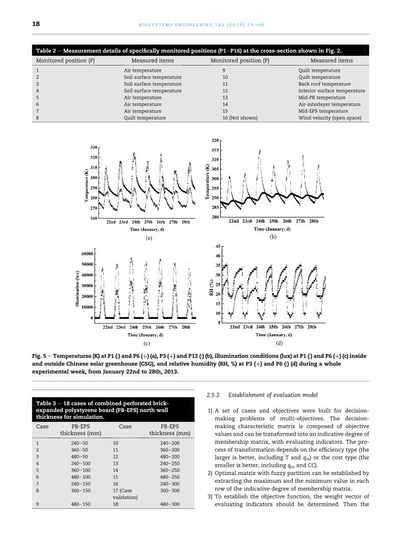
January 22nd to 28th). Figure 5 shows the full data set of

temperatures (P1, P3, P6 and P12), illumination conditions (P1

and P6, recorded by illumination sensor with the valid range

of 0e200,000 lux and precision of ±5%) inside and outside the

CSG, and relative humidity (RH, P3 and P6, recorded by RH

sensor with the valid range of 0e99% and precision of ±3%)

during the whole experimental week with clear days and

nights, which reasonably supported the first and the third

simplifications made in Section 2.2.2. The simulated results

were compared with the measured data to validate the

computer model.

2.4. Model applications

Once the computer simulation was validated, it could be used

to predict the performance of heat retention in terms of

varying thicknesses of north wall, as listed in Table 3. Same

model parameters, initial and boundary conditions and solv-

ing methodology were used in the models.

2.5. Comprehensive evaluation

2.5.1. Structure of evaluation modelStructure of comprehensive evaluation model is shown in

Table 4. Similar evaluation models can also be found else-

where (Jin et al., 2014; Jing, Ng,&Huang, 2007; Li&Hu, 2006; Qi

et al., 2010; Zhou et al., 2007). Three main aspects, which can

be representative for the performance of north wall in CSG,

have been selected to establish the comprehensive evaluation

model for further calculation, including temperatures, abso-

lute heat fluxes in Fig. 6 and the construction cost (CC) in Table

5. All of the simulated data except for CC were obtained from

the model outputs and post processing. CC was derived from

the local construction market in 2013 in Shaanxi Province,

China (Table 5).

Table 2 e Measurement details of specifically monitored positions (P1eP16) at the cross-section shown in Fig. 2.

Monitored position (P) Measured items Monitored position (P) Measured items

1 Air temperature 9 Quilt temperature

2 Soil surface temperature 10 Quilt temperature

3 Soil surface temperature 11 Back roof temperature

4 Soil surface temperature 12 Interior surface temperature

5 Air temperature 13 Mid-PB temperature

6 Air temperature 14 Air-interlayer temperature

7 Air temperature 15 Mid-EPS temperature

8 Quilt temperature 16 (Not shown) Wind velocity (open space)

Fig. 5 e Temperatures (K) at P1 (j) and P6 (þ) (a), P3 (þ) and P12 (j) (b), illumination conditions (lux) at P1 (j) and P6 (þ) (c) inside

and outside Chinese solar greenhouse (CSG), and relative humidity (RH, %) at P3 (þ) and P6 (j) (d) during a whole

experimental week, from January 22nd to 28th, 2013.

Table 3 e 18 cases of combined perforated brick-expanded polystyrene board (PB-EPS) north wallthickness for simulation.

Case PB-EPSthickness (mm)

Case PB-EPSthickness (mm)

1 240e50 10 240e200

2 360e50 11 360e200

3 480e50 12 480e200

4 240e100 13 240e250

5 360e100 14 360e250

6 480e100 15 480e250

7 240e150 16 240e300

8 360e150 17 (Case

validation)

360e300

9 480e150 18 480e300

b i o s y s t em s e n g i n e e r i n g 1 4 2 ( 2 0 1 6 ) 1 2e2 618

2.5.2. Establishment of evaluation model

1) A set of cases and objectives were built for decision-

making problems of multi-objectives. The decision-

making characteristic matrix is composed of objective

values and can be transformed into an indicative degree of

membership matrix, with evaluating indicators. The pro-

cess of transformation depends on the efficiency type (the

larger is better, including T and qin) or the cost type (the

smaller is better, including qex and CC).

2) Optimal matrix with fuzzy partition can be established by

extracting the maximum and the minimum value in each

row of the indicative degree of membership matrix.

3) To establish the objective function, the weight vector of

evaluating indicators should be determined. Then the

Table 4 e Structure of comprehensive evaluationmodel for further calculation of weighted entropy and fuzzy optimisationmethods. The specific positions in the 3rd hierarchy are illustrated in Fig. 6.

The 1st hierarchy The 2nd hierarchy The 3rd hierarchy

Comprehensive evaluation model of north wall in CSG Temperature (T) Inside air temperature (TP6)

Interior wall surface temperature (TP12)

Average wall temperature (Ta)

Absolute heat flux (q) Absolute heat flux of interior wall surface (qin)

Absolute heat flux of exterior wall surface (qex)

Construction cost (CC) Construction cost (CC)

Fig. 6 e Four selected characteristic parameters in the optimised model. TP12 and TP6 are the temperatures measured at

positions of P12 and P6 in Fig. 2.

b i o s y s t em s e ng i n e e r i n g 1 4 2 ( 2 0 1 6 ) 1 2e2 6 19

optimal value of relative membership degree of all the

cases may be deduced, in terms of the criterion of the

minimum summation of quadratic optimal and quadratic

worst weighted Euclidean distances.

4) Comprehensive evaluation model of thermal insulation

properties can be finally received by differentiating the

objective function and assigning zero value to that deriv-

ative. Weight vector of evaluating indicators can be deter-

mined by employingweighted entropymethod, calculating

the degree of memberships with different cases and then

ordering them by using fuzzy optimisation. According to

the maximum entropy principle, the case would be theo-

retically considered as optimal its membership was larger

than the others.

Table 5 e Characteristic values of selected 6 indicators in 18 ca

Case TP6 (K) TP12 (K) Ta (K) qin (W

1 282.6 285.1 283.8 4

2 283.0 286.3 285.9 7

3 283.3 287.0 287.4 8

4 283.8 286.6 284.8 6

5 284.1 287.6 286.8 8

6 284.5 288.4 288.6 9

7 284.0 287.0 284.5 6

8 284.3 288.1 286.8 9

9 284.7 288.7 288.5 9

10 284.5 287.8 285.3 7

11 284.8 288.6 287.0 8

12 285.2 289.3 288.8 10

13 284.7 287.9 284.9 7

14 285.1 288.9 287.1 9

15 285.4 289.5 288.7 10

16 284.8 288.0 285.0 7

17 285.9 289.6 287.4 9

18 286.1 289.6 289.4 10

2.5.3. Characteristic values in the modelAccording to the structure of the comprehensive evaluation

model in Table 4, six characteristic values were carefully

chosen from the results of modelling, which were partly

shown in Fig. 6 and fully listed in Table 5. The CC consists of

unit cost of PB (US$15.81 per 240 mm�1 and m�2), that of EPS

(US$18.25 per 50 mm�1 and m�2) and labour cost.

2.5.4. Optimisation and calculation procedure

1) If n (n ¼ 18 in this paper) was defined as the number of

cases satisfying the constraint conditions, m (m ¼ 6 in this

paper) was defined as the number of indicators to distin-

guish between advantages and disadvantages with

ses for optimising models.

m�2) qex (W m�2) Constructioncost (CC, US$ mm�1 m�2)

9.40 36.61 68.13

5.14 42.74 83.94

7.29 45.86 99.75

1.32 18.33 104.64

1.23 21.38 120.45

5.17 22.94 136.26

7.38 10.43 141.15

0.07 13.52 156.96

9.48 13.63 172.77

5.19 3.95 177.65

8.49 9.14 193.46

0.77 9.93 209.27

1.84 5.79 214.16

2.79 8.08 229.97

1.37 7.69 245.78

3.27 6.04 250.67

1.32 7.11 266.48

2.43 7.55 282.29

b i o s y s t em s e n g i n e e r i n g 1 4 2 ( 2 0 1 6 ) 1 2e2 620

evaluating objective, the decision-making characteristic

matrix X, with n cases and m indicators, could be obtained

as follows:

X ¼ xij

� �(8)

where xij is the characteristic value for indicator i and case j,

i ¼ 1, 2,…, m; j ¼ l, 2,…, n. All the values in matrix X are given

in Table 5.

2) Generally, evaluating indicators of comprehensive perfor-

mance with north wall can be divided into the efficiency

and cost types when optimising. To calculate the relative

membership, computational equations for these two types

of indicators are:

rij ¼�xij � xi min

�=ðxi max � xi minÞ for efficiency type (9)

rij ¼�xi max � xij

�=ðxi max � xi minÞ for cost type (10)

where ximax is themaximum characteristic value of indicator i;

ximin is the minimum characteristic value of indicator i.

Decision-making characteristic matrix X can be trans-

formed into an indicative degree of membership matrix R

according to Eqs. (9) and (10):

R ¼ �rij�

(11)

where rij is the characteristic value for the relative member-

ship with indicator i and case j.

The indicative degree of membership matrix B can be got

after normalising matrix R:

B ¼ �bij

�(12)

where bij is the normalised characteristic value.

The optimal relative membership degree G and the worst

relativemembership degreeDwithin n cases can be defined as

follows:

Table 6 e Indicative membership matrix R andnormalised matrix B (i ¼ 1, 2, …, m; j ¼ l, 2, …, n).

Matrix R (Matrix B)i

j

0.000 0.000 0.000 0.000 0.221 1.000

0.105 0.259 0.382 0.485 0.074 0.926

0.199 0.417 0.648 0.715 0.000 0.852

0.322 0.330 0.181 0.225 0.657 0.830

0.419 0.548 0.542 0.600 0.584 0.756

0.519 0.718 0.864 0.863 0.547 0.682

0.379 0.419 0.136 0.339 0.845 0.659

0.479 0.650 0.549 0.767 0.772 0.585

0.578 0.785 0.842 0.944 0.769 0.511

0.527 0.585 0.273 0.486 1.000 0.489

0.627 0.763 0.571 0.737 0.876 0.415

0.724 0.916 0.908 0.969 0.857 0.341

0.590 0.614 0.197 0.423 0.956 0.318

0.695 0.843 0.598 0.818 0.901 0.244

0.786 0.971 0.890 0.980 0.911 0.170

0.618 0.643 0.214 0.450 0.950 0.148

0.940 0.998 0.655 0.790 0.925 0.074

1.000 1.000 1.000 1.000 0.914 0.000

G ¼ �g1; g2; ,,,; gm

�T(13)

D ¼ ðd1;d2;/;dmÞT (14)

where gi ¼ ∨nj¼1 rij and di ¼ ∧n

j¼1 rij. The symbols used here (∨, ∧)mean that the extreme values (maximum value, minimum

value) are expected to be chosen through the definitions (Qi

et al., 2010; Qin, 2003; Zhou et al., 2007).

Indicative membership matrix R and normalised matrix B

can be acquired by Eqs. (9) and (10), as presented in Table 6.

B is same as R because of the Eqs. (13) and (14) are as

follows:

G ¼ ð1; 1; 1; 1; 1; 1 ÞT and D ¼ ð0; 0; 0; 0; 0; 0 ÞT

3) Entropy value Hi can be determined as follows:

Hi ¼ � 124Xn

fij ln fij

35 (15)

ln nj¼1

fij ¼bijPnt¼1 bit

(16)

where 0 � Hi � 1, fij is an incoming function, fij ln fij ¼ 0 was

assumed to validate ln fij when fij ¼ 0, i ¼ 1, 2,…, m; j ¼ 1, 2,…,

n.

Therefore, vector quantity of entropy value H can be

computed by Eqs. (15) and (16):

H ¼ ð 0:948; 0:960; 0:933; 0:958; 0:953; 0:927 ÞT

Obviously, the average entropy values of evaluation model

is 94.7%, whichmay possibly explain the reason that all of the

indicators can represent the majority of original information

(Zhang, Zhang, & Chi, 2010).

Weight entropy of evaluating indicator Wei can be calcu-

lated as follows:

wei ¼ 1�Hi

m�Pmi¼1 Hi

(17)

where i ¼ 1, 2, …, m. Therefore, vector quantity of weighted

entropy We can be computed by Eq. (17):

we ¼ ð0:162; 0:125; 0:208; 0:131; 0:146; 0:228 ÞT

4) Membership uj of case j can be achieved by adopting

weighted and generalised Euclidean distance method and

the least square method:

8>>< Pm �wei

�gi � rij

��29>>=

uj ¼ >>:1þ i¼1Pm

i¼1

�wei

�rij � di

��2>>;(18)

Therefore, vector quantity of relative membership degree

U with 18 cases can be achieved by Eq. (18). This relative de-

gree of membership was compared for the 18 cases listed in

b i o s y s t em s e ng i n e e r i n g 1 4 2 ( 2 0 1 6 ) 1 2e2 6 21

Table 5 and used to guide the optimal selection of the designed

north wall.

3. Results and discussions

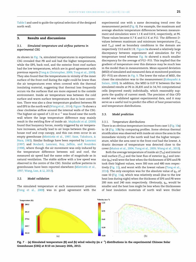
3.1. Simulated temperature and airflow patterns inexperimental CSG

As shown in Fig. 7a, simulated temperatures in experimental

CSG revealed that PB and soil had the higher temperatures,

while the EPS, back roof, and the exterior front roof surface

had the low temperatures, which are in good agreement with

previous reports (Tong & Christopher, 2009; Tong et al., 2009).

They also found that the temperatures in vicinity of the inner

surface of the front roof during the night could be lower than

the air temperatures even when covered with the thermal

insulating material, suggesting that thermal loss frequently

occurs via the surfaces that are more exposed to the outside

environment. Inside air temperature was between the cold

surface and warm surface temperatures due to heat convec-

tion. There was also a clear temperature gradient between PB

and EPS in the northwall (Wang et al., 2014). Figure 7b shows a

clear clockwise airflow around the internal walls of the CSG.

The highest air speed of 1.22 m s�1 was found near the north

wall where the large temperature difference may mainly

result in the swirling flow of inside air. Majdoubi et al. (2009)

found that buoyancy forces, mostly triggered by air tempera-

ture increases, actually lead to air loops between the green-

house roof and crop canopy, and this can even occur in an

empty greenhouse (Mistriotis et al., 1997; Sase, Takakura, &

Nara, 1983). Similar findings have been reported by Lamrani

(1997) and Boulard, Lamrani, Roy, Jaffrin, and Bouirden

(1998), where though the air movement was only induced by

the temperature difference between soil and roof, the

measured air speed had the same order of magnitude as in

natural ventilation. The stable airflow with a low speed was

observed in the centre of the CSG. Similar airflow patterns in

greenhouses have been reported elsewhere (Mistriotis et al.,

1997; Wang, Luo, & Li, 2013).

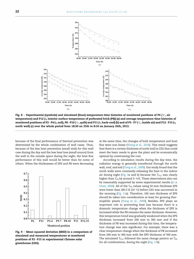
3.2. Model validation

The simulated temperature at each measurement position

(Tong et al., 2009) was in good agreement with the

Fig. 7 e (a) Simulated temperature (K) and (b) wind velocity (m s

Greenhouse (CSG) at 8:10 on January 26th, 2013.

experimental one with a same decreasing trend over the

measurement period (Fig. 8). For example, the maximum and

average absolute temperature differences between measure-

ment and simulation were 1.1 K and 0.8 K, respectively, at P6.

These values became 0.7 K and 0.2 K at P12. The different D-

values between maximum and minimum temperatures (Tsky

and Tsoil) used as boundary conditions in the domain are

respectively 13.0 and 8.1 K. Figure 8a showed a relatively large

discrepancy between experiment and simulation for P12

temperature trend whereas Fig. 8c showed a much smaller

discrepancy for the average of P12eP15. This implied that the

gradient of temperature over this distance may be much less

in the model than in measurements. Mean squared deviation

(MSD) of simulated andmeasured data at monitored positions

(P2eP15) are shown in Fig. 9. The lower the value of MSD, the

closer the simulation was to the measurement (Kobayashi &

Salam, 2000). In addition, the MSD is 0.07 K between the two

simulated results at P6 in 26,835 and in 54,741 computational

cells (improved mesh) individually, which reasonably sup-

ports the quality of current mesh. The precision of this CFD

model was validated against experimental data, and it may

serve as a useful tool to predict the effect of heat preservation

and temperature distributions.

3.3. Model prediction

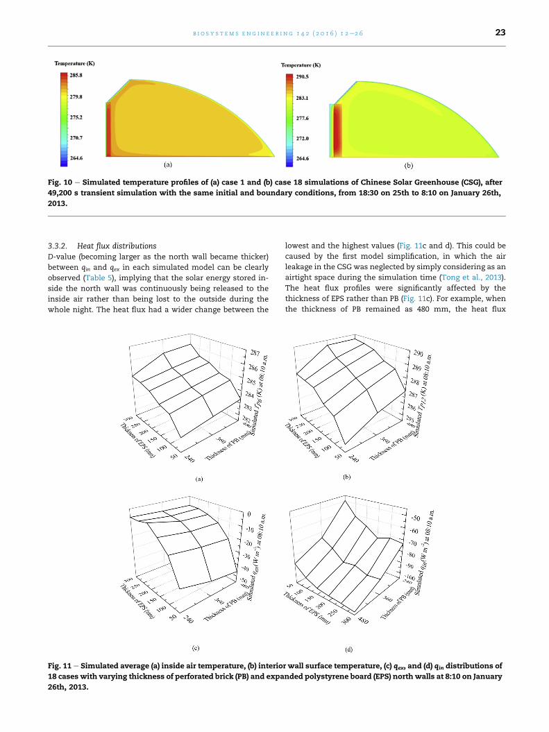
3.3.1. Temperature distributionsThere is an obvious temperature increase from case 1 (Fig. 10a)

to 18 (Fig. 10b) by comparing profiles. Some obvious thermal

stratificationwas observedwith inside air since the area in the

immediate vicinity of the north wall had the higher temper-

ature, whilst the area next to the front roof had the lowest. A

drastic decrease of temperature was detected close to the

cover (Mu~noz et al., 2004; Tong et al., 2009; Wang et al., 2013).

Both the average temperature of inside air (TP6) and interior

wall surface (TP12) and the heat flux of exterior (qex) and inte-

rior (qin) wall were the best when the thicknesses of EPS and PB

took their highest values, were 300 mm and 480 mm respec-

tively (Fig. 11), and worst with the lowest values (Tong et al.,

2014). The only exception was for the absolute value of qex of

case 10 (Fig. 11a), which was relatively small (due to the low

heat loss during night) when the thickness of EPS and PB were

200 mm and 240 mm respectively. Obviously, qex would be

smaller and the heat loss might be less when the thicknesses

of heat insulation materials of north wall were thicker

¡1) distributions in the experimental Chinese Solar

18:00 20:00 22:00 00:00 02:00 04:00 06:00 08:00

284

286

288

290

292

294

296

Tem

pera

ture

(K)

Time (h)

18:00 20:00 22:00 00:00 02:00 04:00 06:00 08:00

282

284

286

288

290

292

294

296

Ave

rage

tem

pera

ture

(K)

Time (h)

18:00 20:00 22:00 00:00 02:00 04:00 06:00 08:00280

282

284

286

288

290

292

294

Ave

rage

tem

pera

ture

(K)

Time (h)

(b) (c)

(a)

Fig. 8 e Experimental (symbols) and simulated (lines) temperature-time histories of monitored positions of P6 (7, air

temperature) and P12 (▫, interior surface temperature of perforated brick (PB)) (a) and average temperature-time histories of

monitored positions of P2eP4 (▫, soil), P8eP10 (7, quilt) and P11 (⋄, back-roof) (b) and of P5eP7 (7, inside air) and P12eP15 (▫,

north wall) (c) over the whole period from 18:30 on 25th to 8:10 on January 26th, 2013.

b i o s y s t em s e n g i n e e r i n g 1 4 2 ( 2 0 1 6 ) 1 2e2 622

because of the final performance of thermal prevention was

determined by the whole combination of wall cases. Thus,

because of the less heat prevention (small sink) for this wall

case during the day and the less heat loss (small source) from

the wall to the outside space during the night, the heat flux

performance of this wall would be better than for some of

others. When the thicknesses of EPS and PB were decreasing

P6 P12 P2-4 P5-7 P8-10 P11 P12-150.0

0.1

0.2

0.3

0.4

0.5

0.6

0.7

MSD

Monitored position

Fig. 9 e Mean squared deviation (MSD) in a comparison of

simulated and measured temperatures at monitored

positions of P2eP15 in experimental Chinese solar

greenhouse (CSG).

at the same time, the changes of both temperature and heat

flux were non-linear (Wang et al., 2014). This result suggests

that there is a certain thickness of northwall in CSG that could

meet the basic needs to grow the plant and be economically

optimal by constraining the cost.

According to simulation results during the day time, the

radiation energy is generally transferred through the north

wall, roof, and soil (Tong et al., 2009). Our study found that the

north walls were constantly releasing the heat to the indoor

air during night (Fig. 9a and b) because the TP12 was clearly

higher than TP6 by around 3e4 K. These observations also can

be reasonably supported by some experimental results (Li &

Chen, 2006). All of the TP6 values using 50 mm thickness EPS

were lower than 283.5 K (10 �C) before CSG was uncovered in

the morning (Fig. 11a). Therefore, 100 mm thickness of EPS

should be taken into consideration at least for growing ther-

mophilic plants (Yang et al., 2009). Besides, EPS plays an

important role in preventing heat loss because there is a

dramatic temperature change when the thickness of EPS is

increased while the PB remains the same thickness. However,

this temperature trendwas gradually weakenedwhen the EPS

thickness increased from 200 mm to 300 mm and if the

thickness of PB was increased during this time, the tempera-

ture change was also significant. For example, there was a

clear temperature change when the thickness of PB increased

from 240 mm to 360 mm with the EPS thickness of 300 mm.

The simulated TP12 followed the same change pattern as TP6

for all combinations, during the night (Fig. 11b).

Fig. 10 e Simulated temperature profiles of (a) case 1 and (b) case 18 simulations of Chinese Solar Greenhouse (CSG), after

49,200 s transient simulation with the same initial and boundary conditions, from 18:30 on 25th to 8:10 on January 26th,

2013.

b i o s y s t em s e ng i n e e r i n g 1 4 2 ( 2 0 1 6 ) 1 2e2 6 23

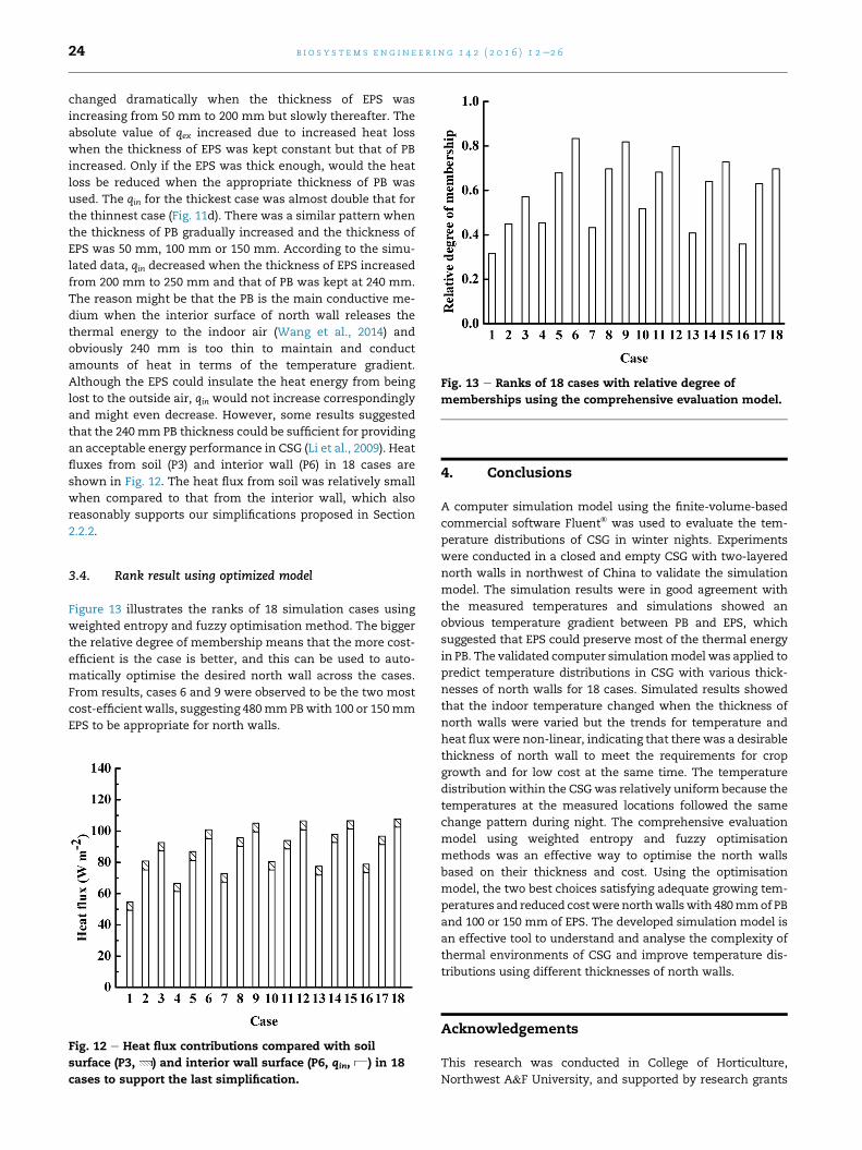
3.3.2. Heat flux distributionsD-value (becoming larger as the north wall became thicker)

between qin and qex in each simulated model can be clearly

observed (Table 5), implying that the solar energy stored in-

side the north wall was continuously being released to the

inside air rather than being lost to the outside during the

whole night. The heat flux had a wider change between the

Fig. 11 e Simulated average (a) inside air temperature, (b) interio

18 cases with varying thickness of perforated brick (PB) and expa

26th, 2013.

lowest and the highest values (Fig. 11c and d). This could be

caused by the first model simplification, in which the air

leakage in the CSG was neglected by simply considering as an

airtight space during the simulation time (Tong et al., 2013).

The heat flux profiles were significantly affected by the

thickness of EPS rather than PB (Fig. 11c). For example, when

the thickness of PB remained as 480 mm, the heat flux

r wall surface temperature, (c) qex, and (d) qin distributions of

nded polystyrene board (EPS) north walls at 8:10 on January

Fig. 13 e Ranks of 18 cases with relative degree of

memberships using the comprehensive evaluation model.

b i o s y s t em s e n g i n e e r i n g 1 4 2 ( 2 0 1 6 ) 1 2e2 624

changed dramatically when the thickness of EPS was

increasing from 50 mm to 200 mm but slowly thereafter. The

absolute value of qex increased due to increased heat loss

when the thickness of EPS was kept constant but that of PB

increased. Only if the EPS was thick enough, would the heat

loss be reduced when the appropriate thickness of PB was

used. The qin for the thickest case was almost double that for

the thinnest case (Fig. 11d). There was a similar pattern when

the thickness of PB gradually increased and the thickness of

EPS was 50 mm, 100 mm or 150 mm. According to the simu-

lated data, qin decreased when the thickness of EPS increased

from 200 mm to 250 mm and that of PB was kept at 240 mm.

The reason might be that the PB is the main conductive me-

dium when the interior surface of north wall releases the

thermal energy to the indoor air (Wang et al., 2014) and

obviously 240 mm is too thin to maintain and conduct

amounts of heat in terms of the temperature gradient.

Although the EPS could insulate the heat energy from being

lost to the outside air, qin would not increase correspondingly

and might even decrease. However, some results suggested

that the 240 mm PB thickness could be sufficient for providing

an acceptable energy performance in CSG (Li et al., 2009). Heat

fluxes from soil (P3) and interior wall (P6) in 18 cases are

shown in Fig. 12. The heat flux from soil was relatively small

when compared to that from the interior wall, which also

reasonably supports our simplifications proposed in Section

2.2.2.

3.4. Rank result using optimized model

Figure 13 illustrates the ranks of 18 simulation cases using

weighted entropy and fuzzy optimisation method. The bigger

the relative degree of membership means that the more cost-

efficient is the case is better, and this can be used to auto-

matically optimise the desired north wall across the cases.

From results, cases 6 and 9 were observed to be the two most

cost-efficient walls, suggesting 480mmPBwith 100 or 150mm

EPS to be appropriate for north walls.

Fig. 12 e Heat flux contributions compared with soil

surface (P3, ) and interior wall surface (P6, qin, ) in 18

cases to support the last simplification.

4. Conclusions

A computer simulation model using the finite-volume-based

commercial software Fluent® was used to evaluate the tem-

perature distributions of CSG in winter nights. Experiments

were conducted in a closed and empty CSG with two-layered

north walls in northwest of China to validate the simulation

model. The simulation results were in good agreement with

the measured temperatures and simulations showed an

obvious temperature gradient between PB and EPS, which

suggested that EPS could preserve most of the thermal energy

in PB. The validated computer simulationmodel was applied to

predict temperature distributions in CSG with various thick-

nesses of north walls for 18 cases. Simulated results showed

that the indoor temperature changed when the thickness of

north walls were varied but the trends for temperature and

heat flux were non-linear, indicating that there was a desirable

thickness of north wall to meet the requirements for crop

growth and for low cost at the same time. The temperature

distribution within the CSGwas relatively uniform because the

temperatures at the measured locations followed the same

change pattern during night. The comprehensive evaluation

model using weighted entropy and fuzzy optimisation

methods was an effective way to optimise the north walls

based on their thickness and cost. Using the optimisation

model, the two best choices satisfying adequate growing tem-

peratures and reduced costwere northwallswith 480mmof PB

and 100 or 150 mm of EPS. The developed simulation model is

an effective tool to understand and analyse the complexity of

thermal environments of CSG and improve temperature dis-

tributions using different thicknesses of north walls.

Acknowledgements

This research was conducted in College of Horticulture,

Northwest A&F University, and supported by research grants

b i o s y s t em s e ng i n e e r i n g 1 4 2 ( 2 0 1 6 ) 1 2e2 6 25

from Special Fund for Agro-Scientific Research in the Public

Interest of Ministry of Agriculture of China (201203002). We

thank all members of Agricultural Engineering Lab for their

helps and Engineer at ANSYS Inc., Mr. Genong Li, for his

remotely technical support. We also thank Associate Professor

Kai Li in College of Water Resources and Architectural Engi-

neering, Northwest A&F University, for his academic advices.

r e f e r e n c e s

Abdel-Ghany, A. M., & Kozai, T. (2006). On the determination ofthe overall heat transmission coefficient and soil heat flux fora fog cooled, naturally ventilated greenhouse: analysis ofradiation and convection heat transfer. Energy Conversion andManagement, 47(15e16), 2612e2628.

ANSYS, F. (2011). User guide 14.0 (Lebanon, NH, USA).Bartzanas, T., Boulard, T., & Kittas, C. (2004). Effect of vent

arrangement on windward ventilation of a tunnel greenhouse.Biosystems Engineering, 88(4), 479e490.

Bierkens, J., & Kappen, H. J. (2014). Explicit solution of relativeentropy weighted control. Systems & Control Letters, 72, 36e43.

Boulard, T., Kittas, C., Roy, J. C., & Wang, S. (2002). Convective andventilation transfers in greenhouses, Part 2: determination ofthe distributed greenhouse climate. Biosystems Engineering,83(2), 129e147.

Boulard, T., Lamrani, M. A., Roy, J. C., Jaffrin, A., & Bouirden, L.(1998). Natural ventilation by thermal effect in a one-half scalemodel mono-span greenhouse. Transactions of the ASAE, 41(3),773e781.

Boulard, T., & Wang, S. (2002). Experimental and numericalstudies on the heterogeneity of crop transpiration in a plastictunnel. Computers and Electronics in Agriculture, 34(1e3),173e190.

Chen, Q. (2008). Progress of practice and theory in sunlightgreenhouse. Journal of Shanghai Jiaotong University (AgriculturalScience), 26(5), 343e350.

De Luca, A., & Termini, S. (1972). A definition of a nonprobabilisticentropy in the setting of fuzzy sets theory. Information andControl, 20(4), 301e312.

Demirel, B. (2013). Optimization of the composite brick composedof expanded polystyrene and pumice blocks. Construction andBuilding Materials, 40, 306e313.

Fang, S., & Gao, Y. (2004). Research on thickness design of thelayer of external insulation complet wall with EPS. Journal ofHeilongjiang Institute of Technology (Natural Science Edition), 18(1),57e59.

Fatnassi, H., Boulard, T., Poncet, C., & Chave, M. (2006).Optimisation of greenhouse insect screening withcomputational fluid dynamics. Biosystems Engineering, 93(3),301e312.

Guias‚u, S. (1971). Weighted entropy. Reports on MathematicalPhysics, 2(3), 165e179.

Guo, S., Sun, J., Shu, S., Lu, X., Tian, J., & Wang, J. (2012). Analysisof general situation, characteristics, existing problems anddevelopment trend of protected horticulture in China. ChinaVegetables, 18, 1e14.

Ji, Y., Huang, G. H., & Sun, W. (2015). Risk assessment ofhydropower stations through an integrated fuzzy entropy-weight multiple criteria decision making method: a case studyof the Xiangxi River. Expert Systems with Applications, 42(12),5380e5389.

Jing, L., Ng, M. K., & Huang, J. Z. (2007). An entropy weighting k-means algorithm for subspace clustering of high-dimensionalsparse data. IEEE Transactions on Knowledge & Data Engineering,19(8), 1026e1041.

Jin, F., Pei, L., Chen, H., & Zhou, L. (2014). Interval-valuedintuitionistic fuzzy continuous weighted entropy and itsapplication to multi-criteria fuzzy group decision making.Knowledge-Based Systems, 59, 132e141.

Kang, S. (1990). Development and improvement for Chinese solargreenhouse of Anshan. Transactions of the CSAE, 6(2), 101e102.

Kobayashi, K., & Salam, M. U. (2000). Comparing simulated andmeasured values using mean squared deviation and itscomponents. Agronomy Journal, 92(2), 345e352.

Lacarri�ere, B., Trombe, A., & Monchoux, F. (2006). Experimentalunsteady characterization of heat transfer in a multi-layerwall including air layersdapplication to vertically perforatedbricks. Energy and Buildings, 38(3), 232e237.

Lamrani, M. A. (1997). Characterisation and modeling of the naturallaminar and turbulent convection and ventilation in a greenhouse (inFrench) (Ph.D. thesis). Agadir, Morocco: University of Agadir.

Lee, I.-B., Bitog, J. P. P., Hong, S.-W., Seo, I.-H., Kwon, K.-S.,Bartzanas, T., et al. (2013). The past, present and future of CFDfor agro-environmental applications. Computers and Electronicsin Agriculture, 93, 168e183.

Lee, I.-B., Sase, S., & Sung, S.-H. (2007). Evaluation of CFD accuracyfor the ventilation study of a naturally ventilated broilerhouse. Japan Agricultural Research Quarterly, 41(1), 53.

Li, J., Bai, Q., & Zhang, Y. (2010). Analysis on measurement of heatabsorption and release of wall and ground in solargreenhouse. Transactions of the CSAE, 26(4), 231e236.

Li, X., & Chen, Q. (2006). Effects of different wall materials on theperformance of heat preservation of wall of sunlightgreenhouse. Chinese Journal of Eco-Agriculture, 14(4), 185e189.

Li, Y., & Hu, Y. (2006). A model of multilevel fuzzy comprehensiveevaluation for investment risk of high and new technologyproject. In Machine Learning and Cybernetics, 2006 InternationalConference on IEEE (pp. 1942e1947) (Dalian, China).

Li, C., Li, Y., & Wen, X. (2009). Temperature characteristics ofNorth Wall covered by polystyrene plate outside solargreenhouse. Journal of Shanxi Agricultural University (NaturalScience Edition), 29(5), 453e457.

Lin, Z., Wen, F., & Zhou, H. (2009). Entropy weight based decision-making theory and its application to black-start decision-making. Proceedings of the CSU EPSA, 21(6), 26e33.

Majdoubi, H., Boulard, T., Fatnassi, H., & Bouirden, L. (2009).Airflow and microclimate patterns in a one-hectare Canarytype greenhouse: an experimental and CFD assisted study.Agricultural and Forest Meteorology, 149(6e7), 1050e1062.

Mirsadeghi, M., C�ostola, D., Blocken, B., & Hensen, J. L. M. (2013).Review of external convective heat transfer coefficient modelsin building energy simulation programs: implementation anduncertainty. Applied Thermal Engineering, 56(1e2), 134e151.

Mistriotis, A., Arcidiacono, C., Picuno, P., Bot, G. P. A., & Scarascia-Mugnozza, G. (1997). Computational analysis of ventilation ingreenhouses at zero- and low-wind-speeds. Agricultural andForest Meteorology, 88(1e4), 121e135.

Molina-Aiz, F. D., Fatnassi, H., Boulard, T., Roy, J. C., & Valera, D. L.(2010). Comparison of finite element and finite volumemethods for simulation of natural ventilation in greenhouses.Computers and Electronics in Agriculture, 72(2), 69e86.

Mu~noz, P., Montero, J., Anton, A., & Iglesias, N. (2004).Computational fluid dynamic modelling of night-time energyfluxes inunheatedgreenhouses.ActaHorticulturae, 691, 403e410.

Norton, T., Sun, D.-W., Grant, J., Fallon, R., & Dodd, V. (2007).Applications of computational fluid dynamics (CFD) in themodelling and design of ventilation systems in theagricultural industry: a review. Bioresource Technology, 98(12),2386e2414.

Qi, F. (2005). The conditions & trends of Chinese greenhouse andequipment industry. Acta Agriculturae Shanghai, 21(1), 53e57.

Qin, S. (2003). Principle and application of comprehensive evaluation.Beijing: Publishing House of Electronics Industry.

b i o s y s t em s e n g i n e e r i n g 1 4 2 ( 2 0 1 6 ) 1 2e2 626

Qi, Y., Wen, F., Wang, K., Li, L., & Singh, S. (2010). A fuzzycomprehensive evaluation and entropy weight decision-making based method for power network structureassessment. International Journal of Engineering, Science andTechnology, 2(5), 92e99.

Sase, S., Takakura, T., & Nara, M. (1983). Wind tunnel testing onairflow and temperature distribution of a naturally ventilatedgreenhouse. In III International Symposium on Energy in ProtectedCultivation 148 (pp. 329e336) (Columbus, USA).

Seo, I.-H., Lee, I.-B., Moon, O.-K., Hong, S.-W., Hwang, H.-S.,Bitog, J. P., et al. (2012). Modelling of internal environmentalconditions in a full-scale commercial pig house containinganimals. Biosystems Engineering, 111(1), 91e106.

Swinbank, W. C. (1963). Long-wave radiation from clear skies.Quarterly Journal of the Royal Meteorological Society, 89(381),339e348.

Teferra, K., Shields, M. D., Hapij, A., & Daddazio, R. P. (2014).Mapping model validation metrics to subject matter expertscores for model adequacy assessment. Reliability Engineering& System Safety, 132, 9e19.

Tong, G., & Christopher, D. (2009). Simulation of temperaturevariations for various wall materials in Chinese solargreenhouses using computational fluid dynamics. Transactionsof the CSAE, 25(3), 153e157.

Tong, G., Christopher, D., & Li, B. (2009). Numerical modelling oftemperature variations in a Chinese solar greenhouse.Computers and Electronics in Agriculture, 68(1), 129e139.

Tong, G., Christopher, D., Li, T., & Wang, T. (2013). Passive solarenergy utilization: a review of cross-section buildingparameter selection for Chinese solar greenhouses. Renewableand Sustainable Energy Reviews, 26, 540e548.

Tong, G., Christopher, D., Zhao, R., Wang, J., & Zhang, Y. (2014).Temperature variations in Chinese solar greenhouses withdifferent wall material thicknesses. Xinjiang AgriculturalSciences, 51(6), 999e1007.

Tong, G., Li, B., Christopher, D., & Yamaguchi, T. (2007).Preliminary study on temperature pattern in China solargreenhouse using computational fluid dynamics. Transactionsof the CSAE, 23(7), 178e185.

Versteeg, H. K., & Malalasekera, W. (1995). An introduction tocomputational fluid dynamics. London: Longman Group Ltd.

Wang, Q., Chen, J., Sun, Z., Zhao, Y., Wu, M., Yang, X., et al.(2010). Heat flux analysis of inner surface of north wall insolar greenhouse. Chinese Journal of Agrometeorology, 31(2),225e229.

Wang, J., Li, S., Guo, S., Ma, C., Wang, J., & Jin, S. (2014).Simulation and optimization of solar greenhouses inNorthern Jiangsu Province of China. Energy and Buildings, 78,143e152.

Wang, X., Luo, J., & Li, X. (2013). CFD based study ofheterogeneous microclimate in a typical Chinese greenhousein central China. Journal of Integrative Agriculture, 12(5),914e923.

Wei, X., Qi, F., Ding, X., Bao, S., Li, Z., & He, F. (2010). Mainachievements in China facility horticulture. Journal ofAgricultural Mechanization Research, 32(12), 227e231.

Wu, J., & Zhang, Q. (2011). Multicriteria decision making methodbased on intuitionistic fuzzy weighted entropy. Expert Systemswith Applications, 38(1), 916e922.

Yang, Q. (2012). Energy efficient heating technologies and modelsin lean-to Chinese solar greenhouses: a review. In IVInternational Symposium on Models for Plant Growth,Environmental Control and Farm Management in ProtectedCultivation (pp. 83e89) (Nanjing, China).

Yang, J., Zou, Z., Zhang, Z., Wang, Y., Zhang, Z., & Yan, F. (2009).Optimization of earth wall thickness and thermal insulationproperty of solar greenhouse in Northwest China. Transactionsof the CSAE, 25(8), 180e185.

Zadeh, L. A. (1968). Probability measures of fuzzy events. Journal ofMathematical Analysis and Applications, 23(2), 421e427.

Zerihun Desta, T., Janssens, K., Van Brecht, A., Meyers, J.,Baelmans, M., & Berckmans, D. (2004). CFD for model-basedcontroller development. Building and Environment, 39(6),621e633.

Zhang, S., Zhang, M., & Chi, G. (2010). The science and technologyevaluation model based on entropy weight and empiricalresearch during the10th five-year of China. Chinese Journal ofManagement, 7(1), 34e42.

Zhou, H., Zhang, G., & Wang, G. (2007). Multi-objective decisionmaking approach based on entropy weights for reservoir floodcontrol operation. Journal of Hydraulic Engineering, 38(1),100e106.