University of Tennessee, Knoxville University of Tennessee, Knoxville TRACE: Tennessee Research and Creative TRACE: Tennessee Research and Creative Exchange Exchange Masters Theses Graduate School 5-2004 CFD Modeling of Dynamic Inlet Flow Distortion Generation CFD Modeling of Dynamic Inlet Flow Distortion Generation Keith Patrick Savage University of Tennessee - Knoxville Follow this and additional works at: https://trace.tennessee.edu/utk_gradthes Part of the Aerospace Engineering Commons Recommended Citation Recommended Citation Savage, Keith Patrick, "CFD Modeling of Dynamic Inlet Flow Distortion Generation. " Master's Thesis, University of Tennessee, 2004. https://trace.tennessee.edu/utk_gradthes/2179 This Thesis is brought to you for free and open access by the Graduate School at TRACE: Tennessee Research and Creative Exchange. It has been accepted for inclusion in Masters Theses by an authorized administrator of TRACE: Tennessee Research and Creative Exchange. For more information, please contact [email protected].
Transcript
University of Tennessee, Knoxville University of Tennessee, Knoxville
TRACE: Tennessee Research and Creative TRACE: Tennessee Research and Creative
Exchange Exchange
Masters Theses Graduate School
5-2004
CFD Modeling of Dynamic Inlet Flow Distortion Generation CFD Modeling of Dynamic Inlet Flow Distortion Generation
Keith Patrick Savage University of Tennessee - Knoxville
Follow this and additional works at: https://trace.tennessee.edu/utk_gradthes
Part of the Aerospace Engineering Commons
Recommended Citation Recommended Citation Savage, Keith Patrick, "CFD Modeling of Dynamic Inlet Flow Distortion Generation. " Master's Thesis, University of Tennessee, 2004. https://trace.tennessee.edu/utk_gradthes/2179
This Thesis is brought to you for free and open access by the Graduate School at TRACE: Tennessee Research and Creative Exchange. It has been accepted for inclusion in Masters Theses by an authorized administrator of TRACE: Tennessee Research and Creative Exchange. For more information, please contact [email protected].
I am submitting herewith a thesis written by Keith Patrick Savage entitled "CFD Modeling of
Dynamic Inlet Flow Distortion Generation." I have examined the final electronic copy of this
thesis for form and content and recommend that it be accepted in partial fulfillment of the
requirements for the degree of Master of Science, with a major in Aerospace Engineering.
Dr. Gary Flandro, Major Professor
We have read this thesis and recommend its acceptance:
Dr. Frank Collins, Dr. Joseph Majdalani
Accepted for the Council:
Carolyn R. Hodges
Vice Provost and Dean of the Graduate School
(Original signatures are on file with official student records.)
To the Graduate Council:
I am submitting herewith a thesis written by Keith Patrick Savage entitled “CFDModeling of Dynamic Inlet Flow Distortion Generation.” I have examined the finalelectronic copy of this thesis for form and content and recommend that it be accepted inpartial fulfillment of the requirements for the degree of Master of Science, with a major inAerospace Engineering.
We have read this dissertation andrecommend its acceptance:
Dr. Frank Collins
Dr. Joseph Majdalani
Dr. Gary FlandroMajor Professor
Acceptance for the Council:
Anne MayhewVice Provost and Dean of GraduateStudies
(Original signatures are on file with official student records.)
CFD Modeling of Dynamic Inlet Flow DistortionGeneration
A Thesis Presentedfor the Master of Science Degree
The University of Tennessee, Knoxville
Keith Patrick SavageMay 2004
ii
Acknowledgments
I would like to thank my advisory committee for their support and advice in the
course of this study, particularly for Dr. Gary Flandro for putting me on this path and
keeping me on track. His curiosity and enthusiasm kept me from getting discouraged
during the more challenging periods.
Dr. Charles Merkle improved my understanding of CFD and gave me a great deal
of ideas, suggestions and advice on the development of the grid itself and the
A.1 The modified door hinge used by Eddy . . . . . . . . . . . . . . . . . . . . . . . . . . . . . . . . 27
A.2 The Lexan test section used in the Eddy study . . . . . . . . . . . . . . . . . . . . . . . . . . 28
D.1.1 Convergence data for Navier-Stokes calculations for the 30° wedge run . . . . . . 54
D.1.2 Convergence data for Shear Stress Transport calculations, 30° wedge run . . . . 54
D.1.3 Total pressure values for 30° wedge after 10,000 iterations . . . . . . . . . . . . . . . . 55
D.1.4 Average velocity values for 30° wedge after 10,000 iterations . . . . . . . . . . . . . . 55
D.1.5 Comparison of pressure coefficient data for 30° wedge . . . . . . . . . . . . . . . . . . . 56
D.2.1 Convergence data for Navier-Stokes calculations for the 60° wedge run . . . . . . 57
D.2.2 Convergence data for Shear Stress Transport calculations, 60° wedge run . . . . 57
D.2.3 Total pressure values for 60° wedge after 10,000 iterations . . . . . . . . . . . . . . . . 58
D.2.4 Average velocity values for 60° wedge after 10,000 iterations . . . . . . . . . . . . . . 58
D.2.5 Comparison of pressure coefficient data for 60° wedge . . . . . . . . . . . . . . . . . . . 59
viii
D.3.1 Convergence data for Navier-Stokes calculations for the 90° wedge run . . . . . . 60
D.3.2 Convergence data for Shear Stress Transport calculations, 90° wedge run . . . . 60
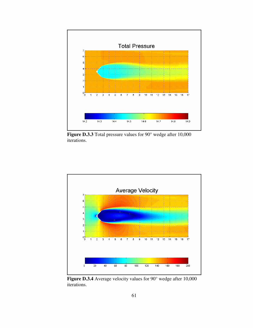
D.3.3 Total pressure values for 90° wedge after 10,000 iterations . . . . . . . . . . . . . . . . 61
D.3.4 Average velocity values for 90° wedge after 10,000 iterations . . . . . . . . . . . . . . 61
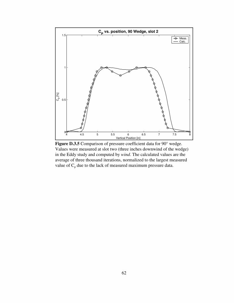
D.3.5 Comparison of pressure coefficient data for 90° wedge . . . . . . . . . . . . . . . . . . . 62
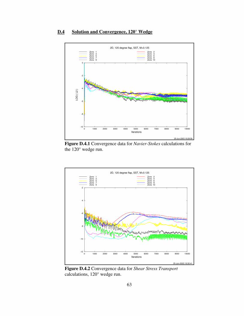
D.4.1 Convergence data for Navier-Stokes calculations for the 120° wedge run . . . . . 63
D.4.2 Convergence data for Shear Stress Transport calculations, 120° wedge run . . . 63
D.4.3 Total pressure values for 120° wedge after 10,000 iterations . . . . . . . . . . . . . . . 64
D.4.4 Average velocity values for 120° wedge after 10,000 iterations . . . . . . . . . . . . . 64
D.4.5 Comparison of pressure coefficient data for 120° wedge . . . . . . . . . . . . . . . . . . 65
D.5.1 Convergence data for Navier-Stokes calculations for the 150° wedge run . . . . . 66
D.5.2 Convergence data for Shear Stress Transport calculations, 150° wedge run . . . 66
D.5.3 Total pressure values for 150° wedge after 10,000 iterations . . . . . . . . . . . . . . . 67
D.5.4 Average velocity values for 150° wedge after 10,000 iterations . . . . . . . . . . . . . 67
D.5.5 Comparison of pressure coefficient data for 150° wedge . . . . . . . . . . . . . . . . . . 68
1
1 Introduction
Jet engines go through many development and testing steps before actually being
installed in an aircraft. Once a bare engine is optimized for ideal operating conditions, it
is submitted to ground tests to evaluate its performance after it is placed in an airframe.
Various methodologies are used in wind tunnel tests to cause distorted flow upstream of
the compressor face to simulate a particular inlet shape. These simulated inlet flow
distortions, at present, only simulate a fixed inlet form over a range of flow velocities.
This is more than adequate for conventional aircraft engines, but high performance
systems like those in military fighter craft have a much broader operating envelope that is
not sufficiently tested with current approaches. Fighter craft are necessarily more
powerful and maneuverable and the latest generation supplements control surfaces with
vectored thrust to enhance that maneuverability even further. These dramatic changes in
orientation distort the inlet flow drastically and briefly, disrupting engine performance
and possibly even damaging components. An additional concern is the transient
disruptions that occur when weapons are released and they and their exhaust gases pass
through the inlet stream. Currently, there is no single, comprehensive and robust
methodology to simulate these situations during wind tunnel testing.
One possible solution to this is the use of an array of individually controlled
wedges placed in the wind tunnel ahead of the engine being tested. This array could
replace existing methods for static testing and allow for more complicated testing as well.
The wedges could be closed completely, causing no significant distortions, then
selectively opened and closed to simulate a transient distortion. Simulated contaminants
could also be introduced to the stream as well, with the wedges providing mixing like the
v-gutters in an afterburner. Taken all together, this wedge array system could replace
existing methodologies while providing an immensely broader range of simulation
possibilities.
Many studies of air flow around bluff bodies have provided a starting point for
mathematical models of wedges, and wind tunnel experiments have corroborated those
results. An obvious next step is to determine if a CFD model can be used to develop the
array.
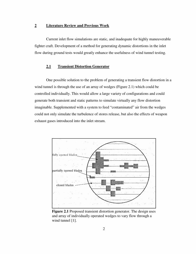
2
Figure 2.1 Proposed transient distortion generator. The design usesand array of individually operated wedges to vary flow through awind tunnel [1].
2 Literature Review and Previous Work
Current inlet flow simulations are static, and inadequate for highly maneuverable
fighter craft. Development of a method for generating dynamic distortions in the inlet
flow during ground tests would greatly enhance the usefulness of wind tunnel testing.
2.1 Transient Distortion Generator
One possible solution to the problem of generating a transient flow distortion in a
wind tunnel is through the use of an array of wedges (Figure 2.1) which could be
controlled individually. This would allow a large variety of configurations and could
generate both transient and static patterns to simulate virtually any flow distortion
imaginable. Supplemented with a system to feed “contaminated” air from the wedges
could not only simulate the turbulence of stores release, but also the effects of weapon
exhaust gases introduced into the inlet stream.
3
2.2 Wake Characteristics
Flow past wedges and other bluff bodies has been well characterized [2-4], as has
flow around aircraft inlets [5, 6]; the ultimate goal is to use the former to simulate the
latter. To verify the basic concept, a study at Virginia Polytechnic Institute developed
mathematical models to represent the wake characteristics of airflow around a wedge.
Then those models were verified with wind tunnel tests, first of a splitter plate, then a
series of individual solid wedges [1]. This was followed by a second study focusing on
more complex arrangements and more measurements being taken closer to the wedge [7].
Using a modified door hinge for the wedges, simple arrays were easily set up and
modified, ultimately showing that wedges could be used to generate consistent and
predictable results.
4
3 CFD Model Setup
A computer-based simulation of the wedge array, based on previous work, that
could be modified and reconfigured “virtually” would greatly assist in developing an
optimal design. To ensure that a CFD model can provide the required results, it should be
shown that a CFD model can re-create the experimental results achieved at Virginia
Polytechnic. Wind was selected as the CFD modeling tool, owing to its flexibility,
applicability and easy access to developers and support. Wind is built from the code of
three older CFD systems; NASTD from McDonnell Douglas, NPARC from the NPARC
Alliance, and NXAIR from AEDC. Taken together, these parts combine to form a very
powerful and comprehensive tool.
Before running wind, a grid must be supplied that includes the relevant wedge
geometry and boundary conditions. Wind allows for a number of different turbulence
models, so an optimal one must be selected. Finally, execution parameters must be set to
mimic the experimental conditions being simulated.
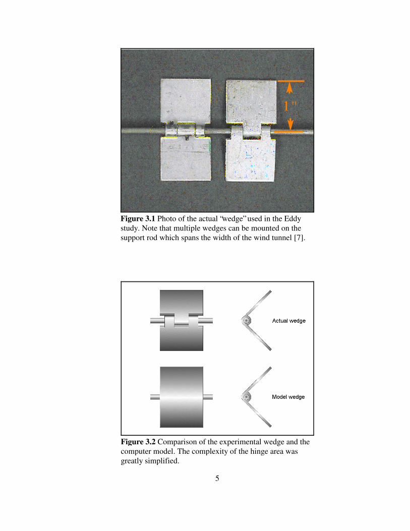
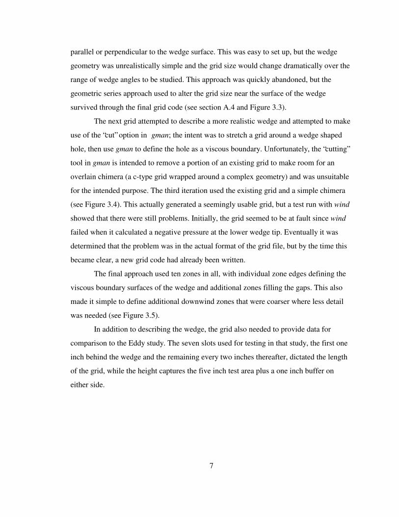
3.1 Wedge Geometry
The wedge used by Eddy started out as a stock steel door hinge [7]. The sixteenth
inch thick hinge was trimmed down to one and an eight inches long and two inches wide
when fully open (see Figure 3.1). The hinge was mounted in the twelve by twelve inch
wind tunnel on a one eighth inch diameter rod (replacing the hinge pin) and then set to a
specific angle and locked into place with set screws on the downwind side of the hinge.
For this study, the wedge model geometry was simplified. The hinge itself was
treated as a smooth, continuous surface on the front and back, and the back of the hinge
merges directly into the “flap” at right angles (see Figure 3.2).
5
Figure 3.1 Photo of the actual “wedge” used in the Eddystudy. Note that multiple wedges can be mounted on thesupport rod which spans the width of the wind tunnel [7].
Figure 3.2 Comparison of the experimental wedge and thecomputer model. The complexity of the hinge area wasgreatly simplified.
6
Because the hinge axis is offset by an eighth of an inch from the upwind surface,
the model must also allow for the hinge area to “shift” from back to front as the wedge
angle decreases. In other words, when the wedge is fully open, the hinge is only exposed
on the back. But as the wedge closes, an increasing part of the hinge is exposed on the
upwind side, while the exposed hinge decreases on the downwind side, e.g. the quarter
cylinder area of the hinge exposed on the upwind edge of the 90° wedge in Figure 3.2.
3.2 Grid Design
At the heart of a CFD model is the grid; an array of points that represent position,
pressure, velocity, and other related data. While tools are available to generate grids, it
seemed more appropriate to build one from scratch for such a relatively simple geometry.
This would provide a good fit and improve the understanding of the results. The wind
reference included an example of Fortran code that would build a three zone Cartesian
structured grid representing a simple 2-D expanding duct [8]. While Fortran is powerful,
it is also a compiled language which can make development of new code time consuming
and visualization and debugging difficult. MatLab is a software product well suited for
computation and visualization with an interpreted programming language designed to
easily handle matrices. This made it an obvious choice for prototyping a grid, while still
leaving the option of later translation to Fortran as needed.
Once a grid is created and saved into an appropriate format, it must be converted
to the “common grid format” used by wind with the cfcnvt tool provided. Then gman is
used to define the boundaries of each zone and preparing the grid for input into wind.
Boundaries that are shared between zones are coupled, while each of the outer boundaries
are defined as freestream, inlet, or outflow and the boundaries of the wedge itself are
defined as viscous walls.
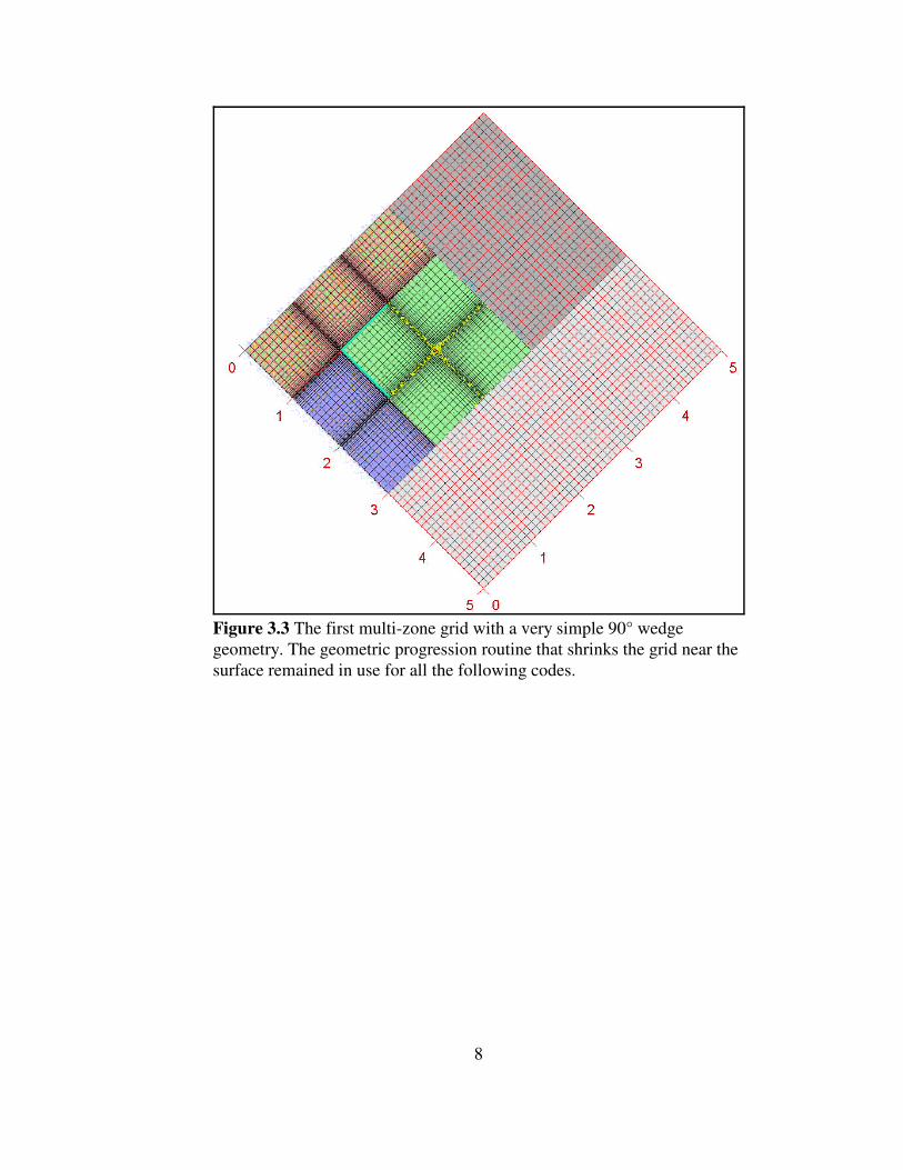
The grid concept went through many changes in the course of development. The
first, simplest grid was just drawn around an angled line, with the grid drawn either
7
parallel or perpendicular to the wedge surface. This was easy to set up, but the wedge
geometry was unrealistically simple and the grid size would change dramatically over the
range of wedge angles to be studied. This approach was quickly abandoned, but the
geometric series approach used to alter the grid size near the surface of the wedge
survived through the final grid code (see section A.4 and Figure 3.3).
The next grid attempted to describe a more realistic wedge and attempted to make
use of the “cut” option in gman; the intent was to stretch a grid around a wedge shaped
hole, then use gman to define the hole as a viscous boundary. Unfortunately, the “cutting”
tool in gman is intended to remove a portion of an existing grid to make room for an
overlain chimera (a c-type grid wrapped around a complex geometry) and was unsuitable
for the intended purpose. The third iteration used the existing grid and a simple chimera
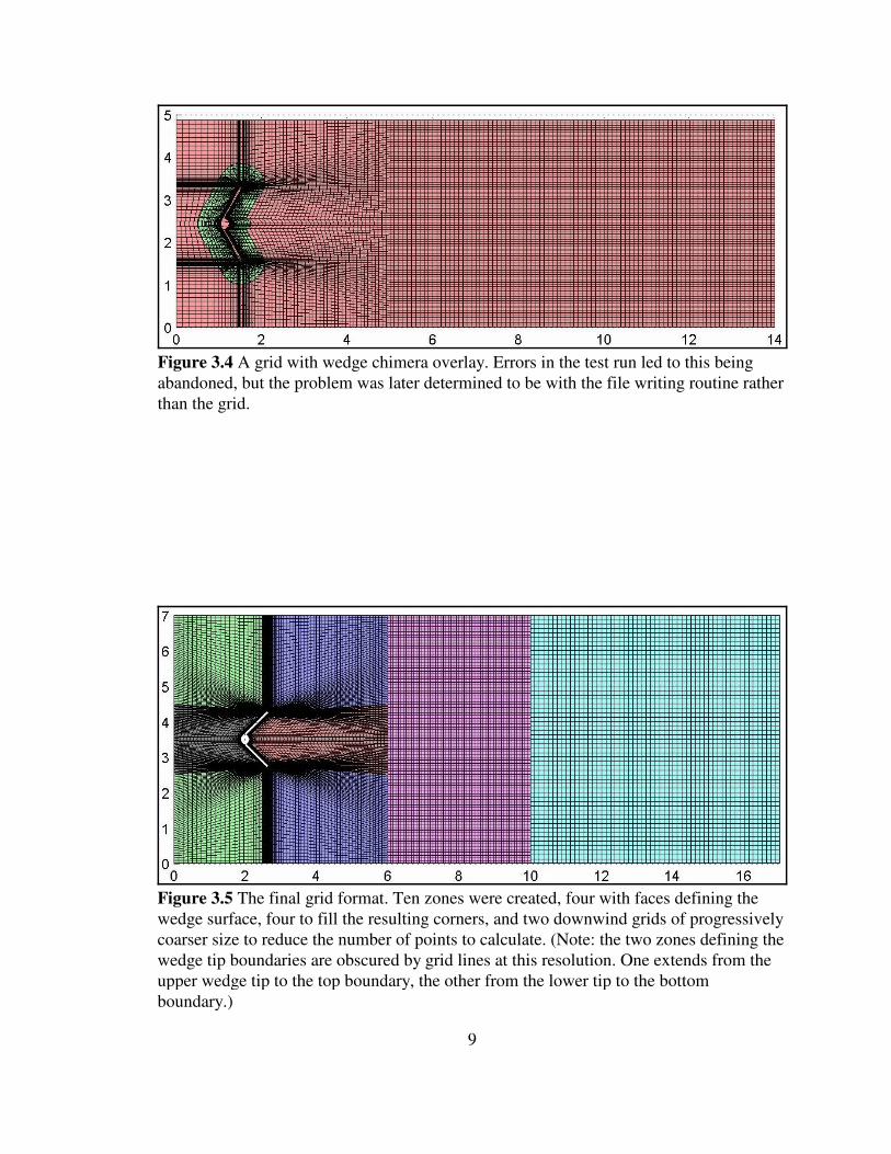
(see Figure 3.4). This actually generated a seemingly usable grid, but a test run with wind
showed that there were still problems. Initially, the grid seemed to be at fault since wind
failed when it calculated a negative pressure at the lower wedge tip. Eventually it was
determined that the problem was in the actual format of the grid file, but by the time this
became clear, a new grid code had already been written.
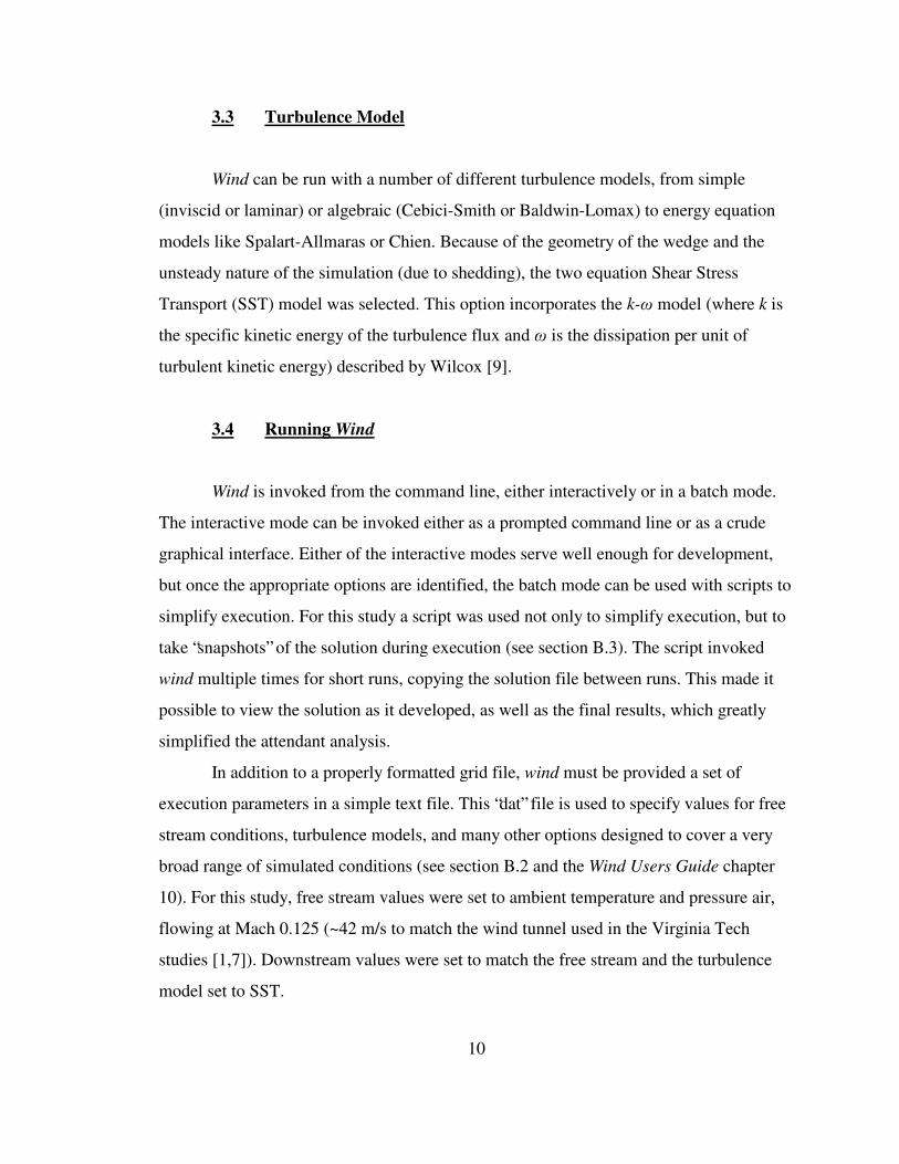
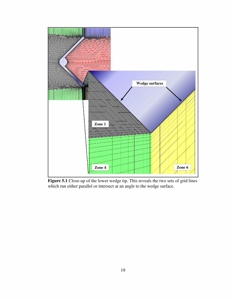
The final approach used ten zones in all, with individual zone edges defining the
viscous boundary surfaces of the wedge and additional zones filling the gaps. This also
made it simple to define additional downwind zones that were coarser where less detail
was needed (see Figure 3.5).
In addition to describing the wedge, the grid also needed to provide data for
comparison to the Eddy study. The seven slots used for testing in that study, the first one
inch behind the wedge and the remaining every two inches thereafter, dictated the length
of the grid, while the height captures the five inch test area plus a one inch buffer on
either side.
8
Figure 3.3 The first multi-zone grid with a very simple 90° wedgegeometry. The geometric progression routine that shrinks the grid near thesurface remained in use for all the following codes.
9
Figure 3.4 A grid with wedge chimera overlay. Errors in the test run led to this beingabandoned, but the problem was later determined to be with the file writing routine ratherthan the grid.
Figure 3.5 The final grid format. Ten zones were created, four with faces defining thewedge surface, four to fill the resulting corners, and two downwind grids of progressivelycoarser size to reduce the number of points to calculate. (Note: the two zones defining thewedge tip boundaries are obscured by grid lines at this resolution. One extends from theupper wedge tip to the top boundary, the other from the lower tip to the bottomboundary.)
10
3.3 Turbulence Model
Wind can be run with a number of different turbulence models, from simple
(inviscid or laminar) or algebraic (Cebici-Smith or Baldwin-Lomax) to energy equation
models like Spalart-Allmaras or Chien. Because of the geometry of the wedge and the
unsteady nature of the simulation (due to shedding), the two equation Shear Stress
Transport (SST) model was selected. This option incorporates the k-& model (where k is
the specific kinetic energy of the turbulence flux and & is the dissipation per unit of
turbulent kinetic energy) described by Wilcox [9].
3.4 Running Wind
Wind is invoked from the command line, either interactively or in a batch mode.
The interactive mode can be invoked either as a prompted command line or as a crude
graphical interface. Either of the interactive modes serve well enough for development,
but once the appropriate options are identified, the batch mode can be used with scripts to
simplify execution. For this study a script was used not only to simplify execution, but to
take “snapshots” of the solution during execution (see section B.3). The script invoked
wind multiple times for short runs, copying the solution file between runs. This made it
possible to view the solution as it developed, as well as the final results, which greatly
simplified the attendant analysis.
In addition to a properly formatted grid file, wind must be provided a set of
execution parameters in a simple text file. This “dat” file is used to specify values for free
stream conditions, turbulence models, and many other options designed to cover a very
broad range of simulated conditions (see section B.2 and the Wind Users Guide chapter
10). For this study, free stream values were set to ambient temperature and pressure air,
flowing at Mach 0.125 (~42 m/s to match the wind tunnel used in the Virginia Tech
studies [1,7]). Downstream values were set to match the free stream and the turbulence
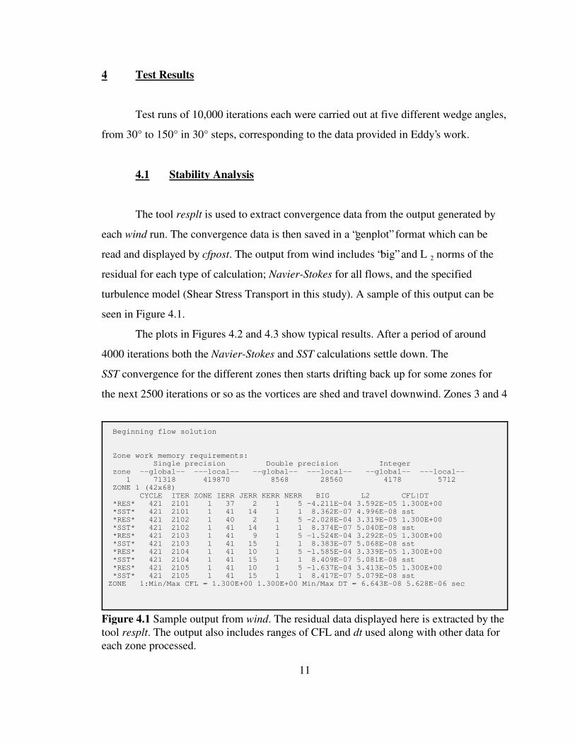
Figure 4.1 Sample output from wind. The residual data displayed here is extracted by thetool resplt. The output also includes ranges of CFL and dt used along with other data foreach zone processed.
4 Test Results
Test runs of 10,000 iterations each were carried out at five different wedge angles,
from 30° to 150° in 30° steps, corresponding to the data provided in Eddy’s work.
4.1 Stability Analysis
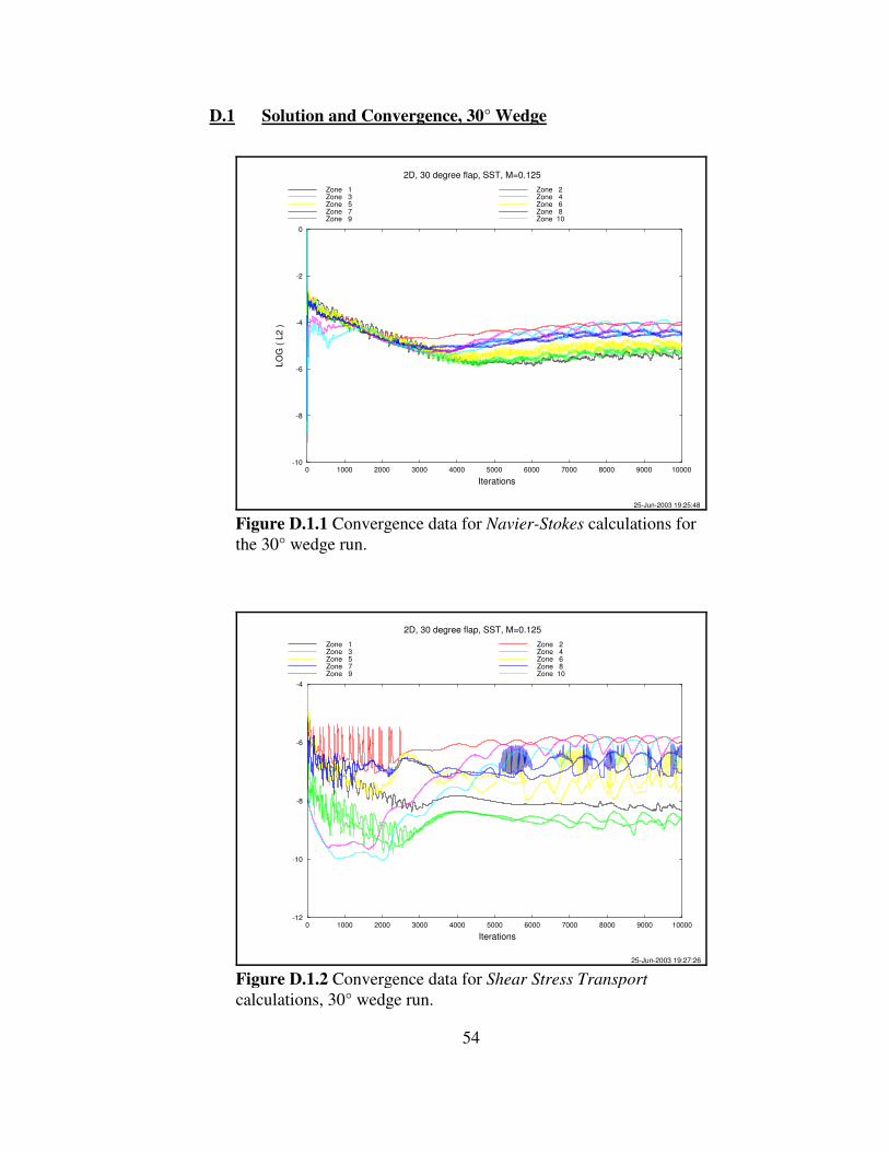
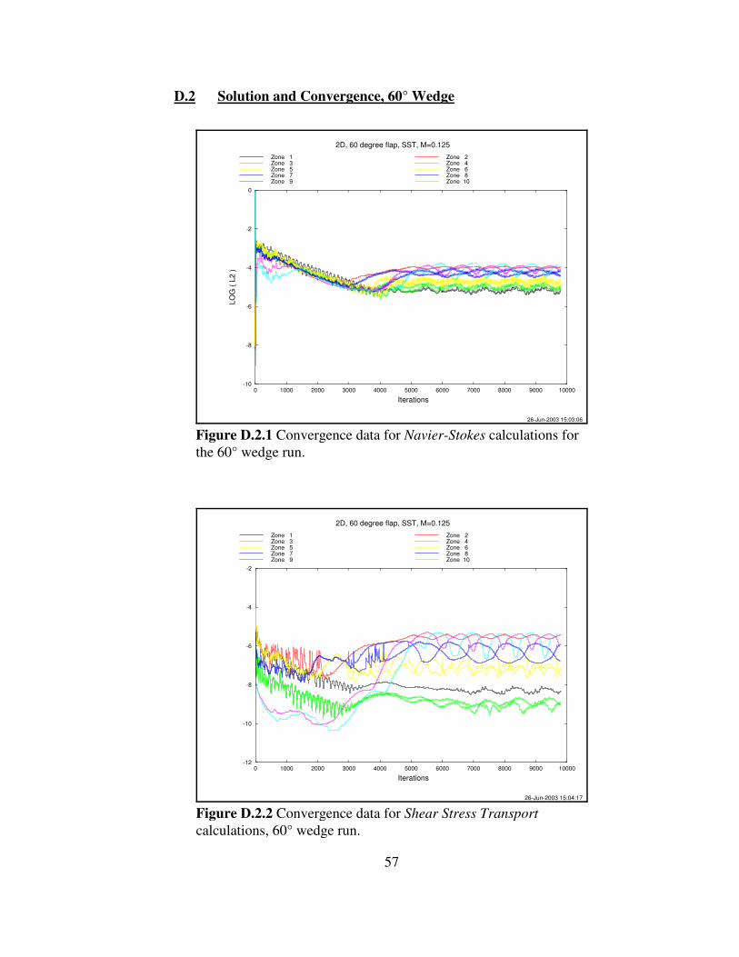
The tool resplt is used to extract convergence data from the output generated by
each wind run. The convergence data is then saved in a “genplot” format which can be
read and displayed by cfpost. The output from wind includes “big” and L norms of the2
residual for each type of calculation; Navier-Stokes for all flows, and the specified
turbulence model (Shear Stress Transport in this study). A sample of this output can be
seen in Figure 4.1.
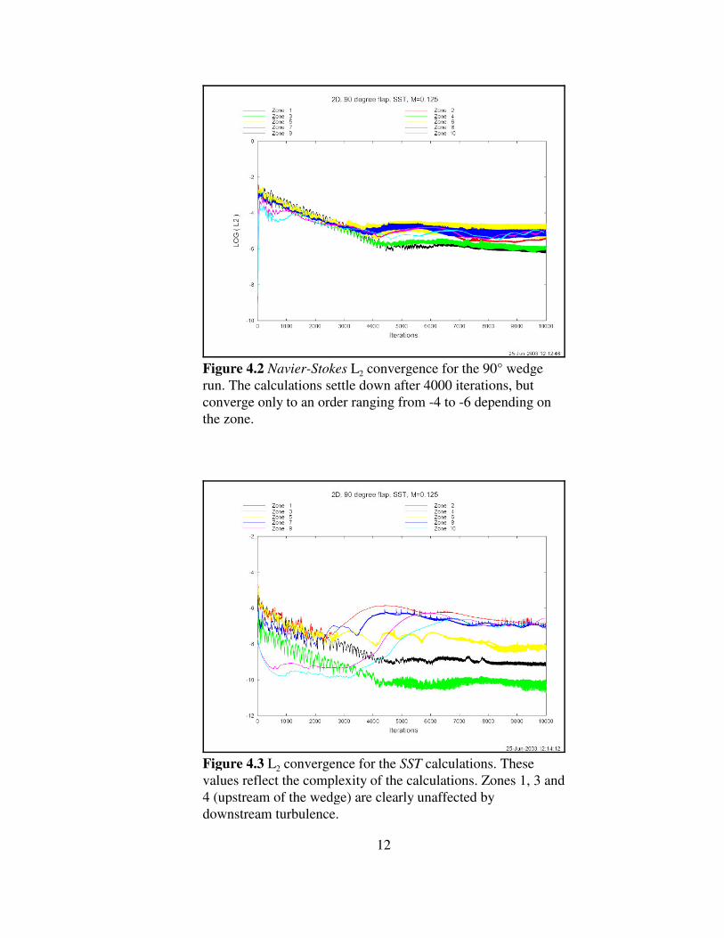
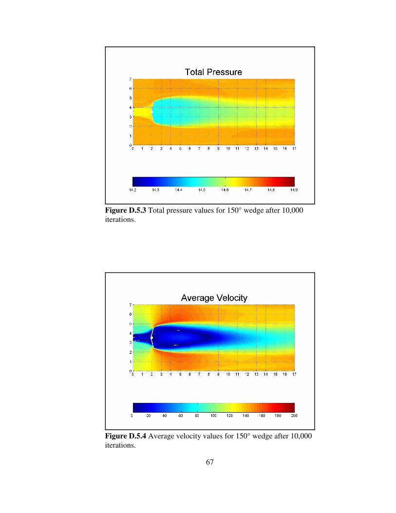
The plots in Figures 4.2 and 4.3 show typical results. After a period of around
4000 iterations both the Navier-Stokes and SST calculations settle down. The
SST convergence for the different zones then starts drifting back up for some zones for
the next 2500 iterations or so as the vortices are shed and travel downwind. Zones 3 and 4
12
Figure 4.3 L convergence for the SST calculations. These2
values reflect the complexity of the calculations. Zones 1, 3 and4 (upstream of the wedge) are clearly unaffected bydownstream turbulence.
Figure 4.2 Navier-Stokes L convergence for the 90° wedge2
run. The calculations settle down after 4000 iterations, butconverge only to an order ranging from -4 to -6 depending onthe zone.
13
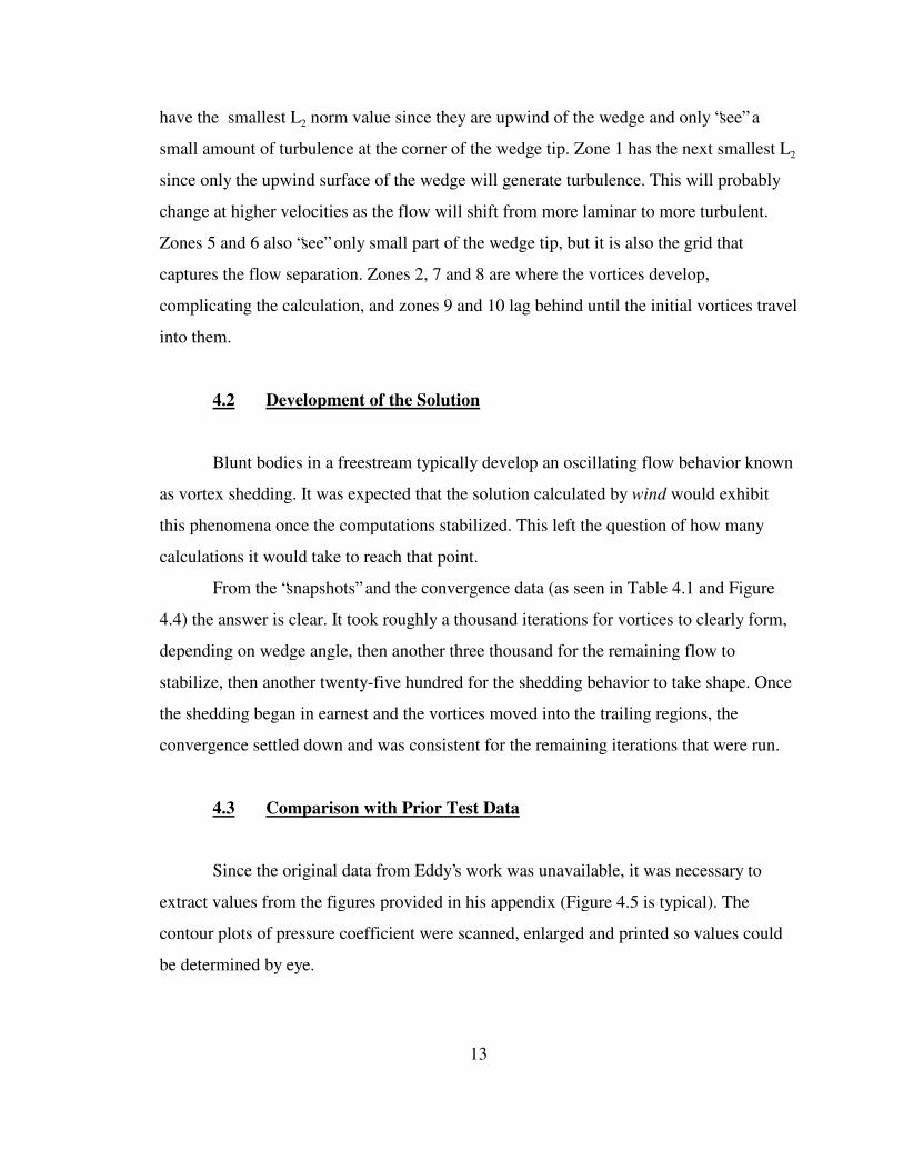
have the smallest L norm value since they are upwind of the wedge and only “see” a2
small amount of turbulence at the corner of the wedge tip. Zone 1 has the next smallest L2
since only the upwind surface of the wedge will generate turbulence. This will probably
change at higher velocities as the flow will shift from more laminar to more turbulent.
Zones 5 and 6 also “see” only small part of the wedge tip, but it is also the grid that
captures the flow separation. Zones 2, 7 and 8 are where the vortices develop,
complicating the calculation, and zones 9 and 10 lag behind until the initial vortices travel
into them.
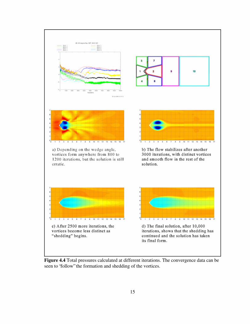
4.2 Development of the Solution
Blunt bodies in a freestream typically develop an oscillating flow behavior known
as vortex shedding. It was expected that the solution calculated by wind would exhibit
this phenomena once the computations stabilized. This left the question of how many
calculations it would take to reach that point.
From the “snapshots” and the convergence data (as seen in Table 4.1 and Figure
4.4) the answer is clear. It took roughly a thousand iterations for vortices to clearly form,
depending on wedge angle, then another three thousand for the remaining flow to
stabilize, then another twenty-five hundred for the shedding behavior to take shape. Once
the shedding began in earnest and the vortices moved into the trailing regions, the
convergence settled down and was consistent for the remaining iterations that were run.
4.3 Comparison with Prior Test Data
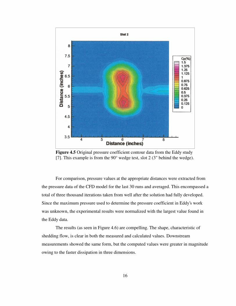
Since the original data from Eddy’s work was unavailable, it was necessary to
extract values from the figures provided in his appendix (Figure 4.5 is typical). The
contour plots of pressure coefficient were scanned, enlarged and printed so values could
be determined by eye.
14
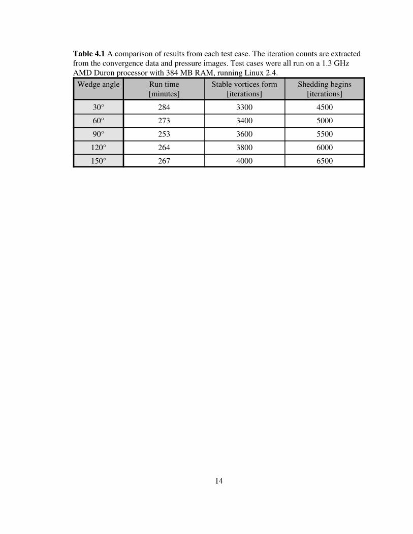
Table 4.1 A comparison of results from each test case. The iteration counts are extractedfrom the convergence data and pressure images. Test cases were all run on a 1.3 GHzAMD Duron processor with 384 MB RAM, running Linux 2.4.
Wedge angle Run time Stable vortices form Shedding begins[minutes] [iterations] [iterations]
30° 284 3300 4500
60° 273 3400 5000
90° 253 3600 5500
120° 264 3800 6000
150° 267 4000 6500
15
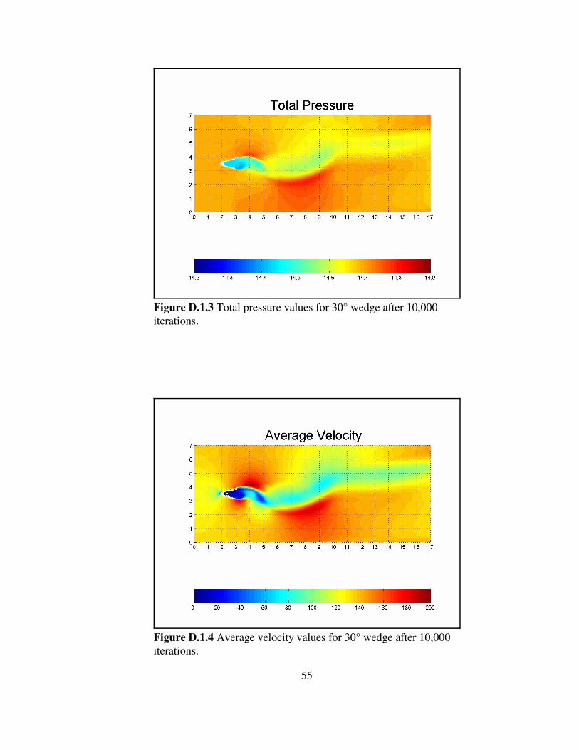
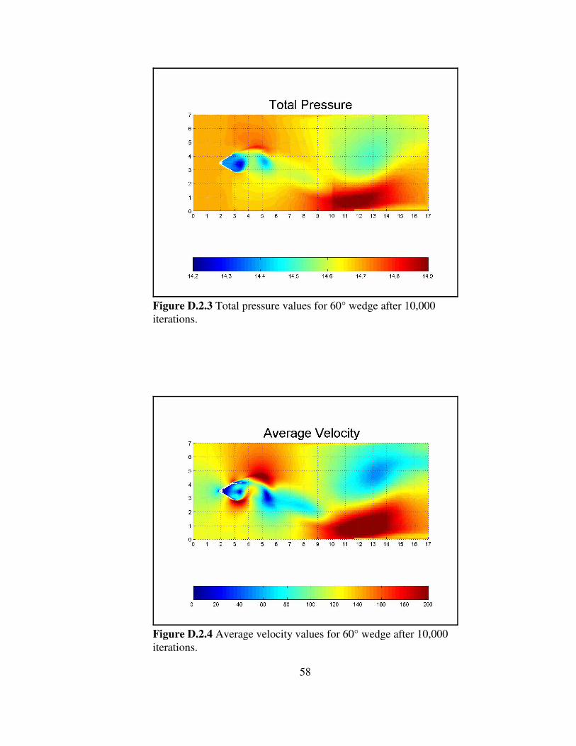
Figure 4.4 Total pressures calculated at different iterations. The convergence data can beseen to “follow” the formation and shedding of the vortices.
16
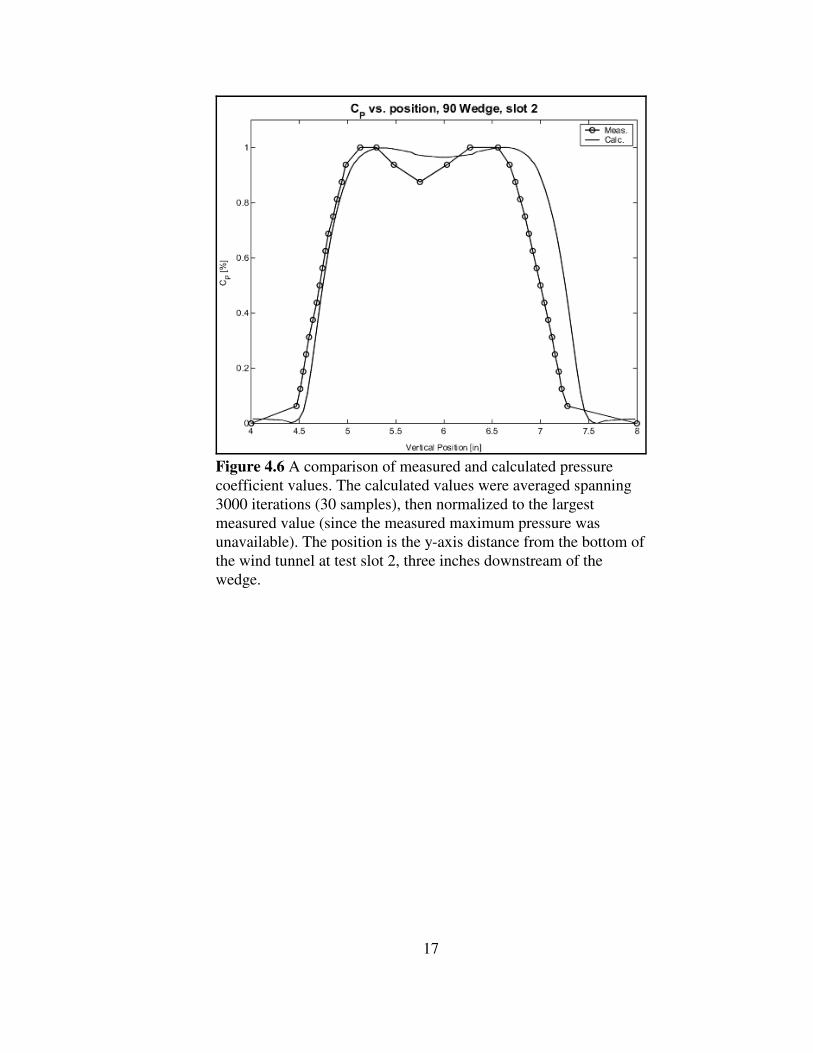
Figure 4.5 Original pressure coefficient contour data from the Eddy study[7]. This example is from the 90° wedge test, slot 2 (3" behind the wedge).
For comparison, pressure values at the appropriate distances were extracted from
the pressure data of the CFD model for the last 30 runs and averaged. This encompassed a
total of three thousand iterations taken from well after the solution had fully developed.
Since the maximum pressure used to determine the pressure coefficient in Eddy’s work
was unknown, the experimental results were normalized with the largest value found in
the Eddy data.
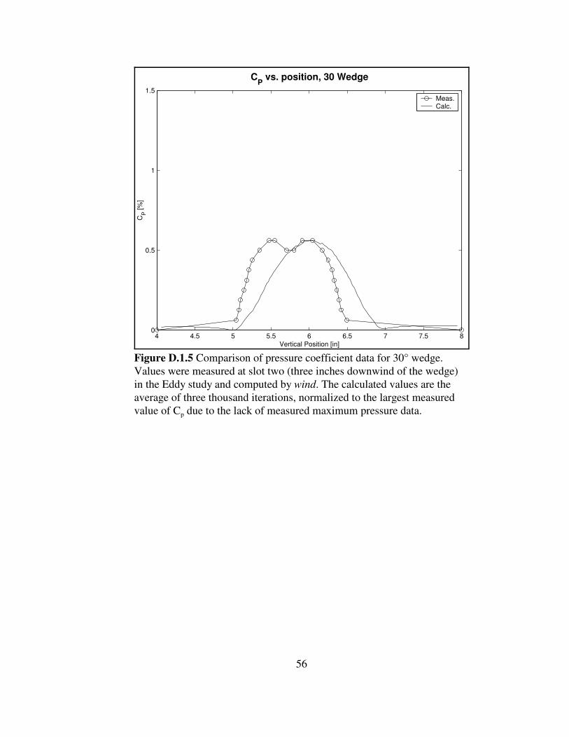
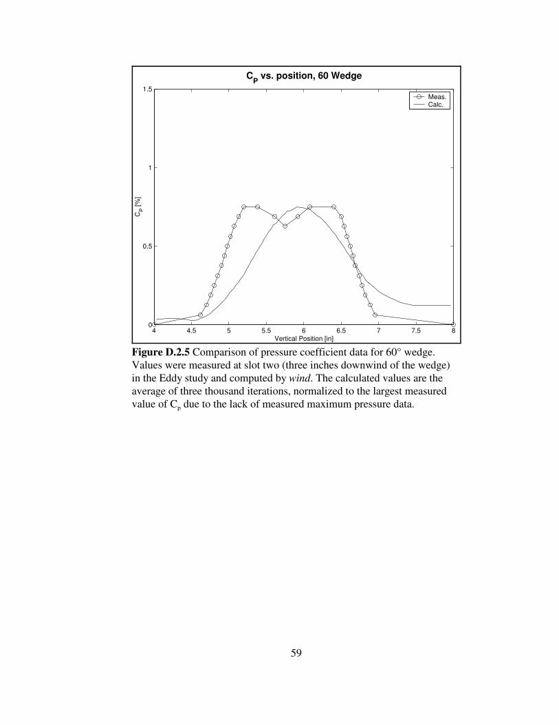
The results (as seen in Figure 4.6) are compelling. The shape, characteristic of
shedding flow, is clear in both the measured and calculated values. Downstream
measurements showed the same form, but the computed values were greater in magnitude
owing to the faster dissipation in three dimensions.
17
Figure 4.6 A comparison of measured and calculated pressurecoefficient values. The calculated values were averaged spanning3000 iterations (30 samples), then normalized to the largestmeasured value (since the measured maximum pressure wasunavailable). The position is the y-axis distance from the bottom ofthe wind tunnel at test slot 2, three inches downstream of thewedge.
18
5 Conclusions and Recommendations
While this study has focused on 2-D, single wedge simulations, it has
demonstrated that the modeling concept is sound and also revealed some possible
limitations of the wedge-as-distortion-generator concept.
5.1 Conclusions
Placing a wedge in a free stream is essentially a bluff-body problem and the CFD
solution showed the classic time dependent vortex shedding behavior expected [2, 10].
Comparing the calculated values to those measured by Eddy showed a good match, right
down to the classic “dimple” in the center.
Because this study only modeled a single wedge in two dimensions, it did not
answer all questions, but it has shown that the model is sound and will prove useful in the
development of a comprehensive and robust simulation of a dynamic distortion generator.
5.2 Recommendations
It may be possible to improve the grid (and achieve better convergence values) by
altering the grid geometry at the wedge tips to curve towards the corners so that the grid
“lines” at the tips are perpendicular, rather than angled (see Figure 5.1). This “body
fitted” approach would help concentrate grid points where the flow separation occurs, at
the leading wedge tip, rather than being spread more uniformly across the upwind surface.
Alternately, the use of chimeras could be re-evaluated, improving the grid at the wedge
tips as well as collapsing zones one through eight into a single background zone and the
chimera. Finally, this study relied on a structured Cartesian grid, but an unstructured
“mesh” grid could well prove to be as effective and more scalable when the work extends
to three dimensions.
Zone 4 Zone 6
Zone 1
Wedge surfaces
19
Figure 5.1 Close-up of the lower wedge tip. This reveals the two sets of grid lineswhich run either parallel or intersect at an angle to the wedge surface.
20
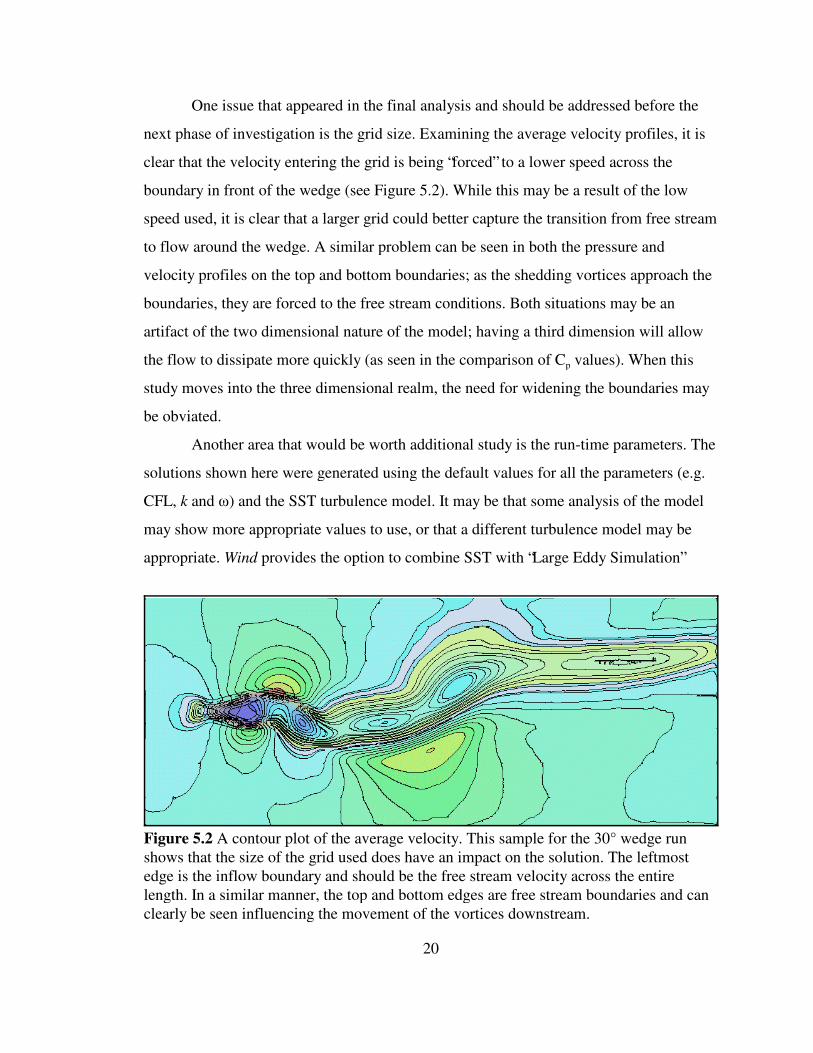
Figure 5.2 A contour plot of the average velocity. This sample for the 30° wedge runshows that the size of the grid used does have an impact on the solution. The leftmostedge is the inflow boundary and should be the free stream velocity across the entirelength. In a similar manner, the top and bottom edges are free stream boundaries and canclearly be seen influencing the movement of the vortices downstream.
One issue that appeared in the final analysis and should be addressed before the
next phase of investigation is the grid size. Examining the average velocity profiles, it is
clear that the velocity entering the grid is being “forced” to a lower speed across the
boundary in front of the wedge (see Figure 5.2). While this may be a result of the low
speed used, it is clear that a larger grid could better capture the transition from free stream
to flow around the wedge. A similar problem can be seen in both the pressure and
velocity profiles on the top and bottom boundaries; as the shedding vortices approach the
boundaries, they are forced to the free stream conditions. Both situations may be an
artifact of the two dimensional nature of the model; having a third dimension will allow
the flow to dissipate more quickly (as seen in the comparison of C values). When thisp
study moves into the three dimensional realm, the need for widening the boundaries may
be obviated.
Another area that would be worth additional study is the run-time parameters. The
solutions shown here were generated using the default values for all the parameters (e.g.
CFL, k and &) and the SST turbulence model. It may be that some analysis of the model
may show more appropriate values to use, or that a different turbulence model may be
appropriate. Wind provides the option to combine SST with “Large Eddy Simulation”
21
which can “...improve predictions of complex flows in a real-world engineering
environment...” [8] and may provide better results than SST alone. On the other hand,
SST may be more sophisticated than is needed for this simulation and a one-equation or
algebraic model might achieve the same results with less processing requirements.
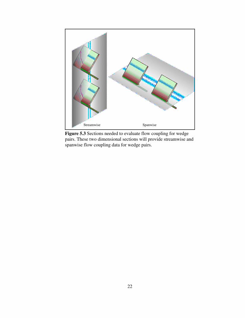
Eddy also studied the turbulence coupling effects of pairs of wedges [7] which
could provide another point of comparison, as well as help determine how multiple
wedges will interact. While the study of spanwise coupling will require a 3D model,
streamwise coupling can be modeled by modifying the grid generation code to include
two edges, one above the other (see Figure 5.3).
In order to produce values for comparison, the wedge geometry and testing
conditions for this study were set to duplicate those in Eddy’s work. This fixed the wedge
size and shape, as well as the free stream velocity, pressure and temperature. Since this
study has shown that the modeling concept is sound, the next step should be to determine
the requirements for the dynamic distortion generator wedge array. These should include
specifications for the range of operating conditions, as well as any constraints that might
influence the wedge design (e.g. the size of available actuators will affect the size of the
wedge and its range of motion).
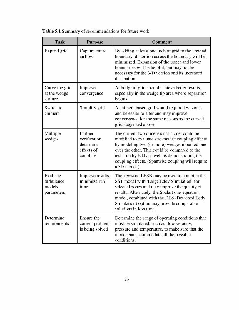
These recommendations are summarized in Table 5.1.
Streamwise Spanwise
22
Figure 5.3 Sections needed to evaluate flow coupling for wedgepairs. These two dimensional sections will provide streamwise andspanwise flow coupling data for wedge pairs.
23
Table 5.1 Summary of recommendations for future work
Task Purpose Comment
Expand grid Capture entire By adding at least one inch of grid to the upwindairflow boundary, distortion across the boundary will be
minimized. Expansion of the upper and lowerboundaries will be helpful, but may not benecessary for the 3-D version and its increaseddissipation.
Curve the grid Improve A “body fit” grid should achieve better results,at the wedge convergence especially in the wedge tip area where separationsurface begins.
Switch to Simplify grid A chimera based grid would require less zoneschimera and be easier to alter and may improve
convergence for the same reasons as the curvedgrid suggested above.
Multiple Further The current two dimensional model could bewedges verification, modified to evaluate streamwise coupling effects
determine by modeling two (or more) wedges mounted oneeffects of over the other. This could be compared to thecoupling tests run by Eddy as well as demonstrating the
coupling effects. (Spanwise coupling will requirea 3D model.)
Evaluate Improve results, The keyword LESB may be used to combine theturbulence minimize run SST model with “Large Eddy Simulation” formodels, time selected zones and may improve the quality ofparameters results. Alternately, the Spalart one-equation
model, combined with the DES (Detached EddySimulation) option may provide comparablesolutions in less time.
Determine Ensure the Determine the range of operating conditions thatrequirements correct problem must be simulated, such as flow velocity,
is being solved pressure and temperature, to make sure that themodel can accommodate all the possibleconditions.
24
References
25
List of References
[1] Jumel, J., King, P.S., and O’Brien, W.F., “Transient Total Distortion Generator
Development, Phase II,” Final Technical Rept. F40600-94-K-0018, Arnold
Engineering Development Center, Tullahoma, TN, July 1999.
[2] Yang, J., Tsai, G., and Wang, W., “Near-Wake Characteristics of Various V-
Shaped Bluff Bodies.” Journal of Propulsion and Power, Vol. 10, No. 1, Jan.-Feb.
1994, pp. 47-55.
[3] Parkinson, G.V. and Jandali, T., “A Wake Source Model for Bluff Body Potential
[9] Wilcox, D.C., Turbulence Modeling for CFD, DCW Industries, 1994, pp. 84-87.
[10] White, F.M., Fluid Mechanics, WCB/McGraw-Hill, 1999, pp. 295-296.
[11] White, F.M., ibid, pp. 427-430.
26
Appendices
27
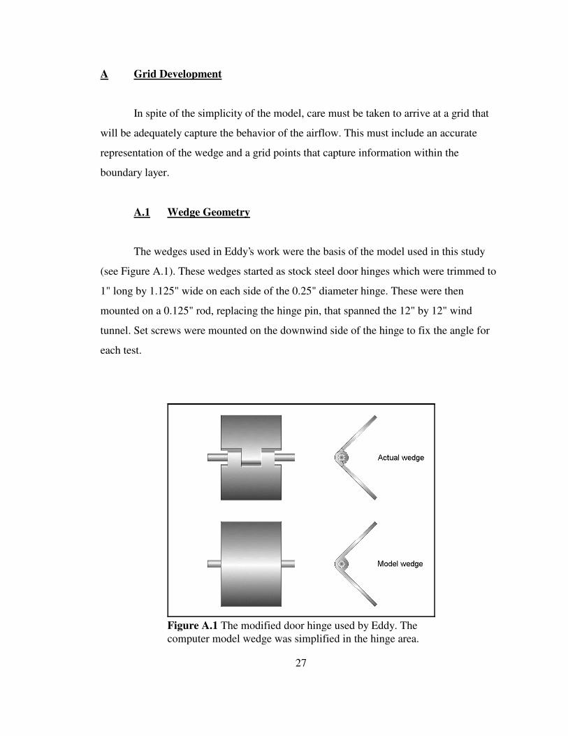
Figure A.1 The modified door hinge used by Eddy. Thecomputer model wedge was simplified in the hinge area.
A Grid Development
In spite of the simplicity of the model, care must be taken to arrive at a grid that
will be adequately capture the behavior of the airflow. This must include an accurate
representation of the wedge and a grid points that capture information within the
boundary layer.
A.1 Wedge Geometry
The wedges used in Eddy’s work were the basis of the model used in this study
(see Figure A.1). These wedges started as stock steel door hinges which were trimmed to
1" long by 1.125" wide on each side of the 0.25" diameter hinge. These were then
mounted on a 0.125" rod, replacing the hinge pin, that spanned the 12" by 12" wind
tunnel. Set screws were mounted on the downwind side of the hinge to fix the angle for
each test.
28
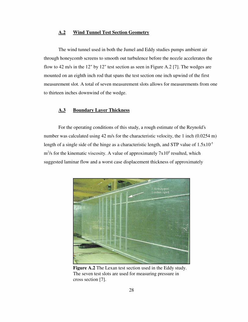
Figure A.2 The Lexan test section used in the Eddy study.The seven test slots are used for measuring pressure incross section [7].
A.2 Wind Tunnel Test Section Geometry
The wind tunnel used in both the Jumel and Eddy studies pumps ambient air
through honeycomb screens to smooth out turbulence before the nozzle accelerates the
flow to 42 m/s in the 12" by 12" test section as seen in Figure A.2 [7]. The wedges are
mounted on an eighth inch rod that spans the test section one inch upwind of the first
measurement slot. A total of seven measurement slots allows for measurements from one
to thirteen inches downwind of the wedge.
A.3 Boundary Layer Thickness
For the operating conditions of this study, a rough estimate of the Reynold’s
number was calculated using 42 m/s for the characteristic velocity, the 1 inch (0.0254 m)
length of a single side of the hinge as a characteristic length, and STP value of 1.5x10⁻⁵
m /s for the kinematic viscosity. A value of approximately 7x10 resulted, which2 4
suggested laminar flow and a worst case displacement thickness of approximately
/x�
5.0
Rex
a�ar�ar 2�ar 3
�á�ar n � 1
a(1r n)1r
arl1r
/max�12
/maxr#/min
1r
29
(A.1)
(A.2)
(A.3)
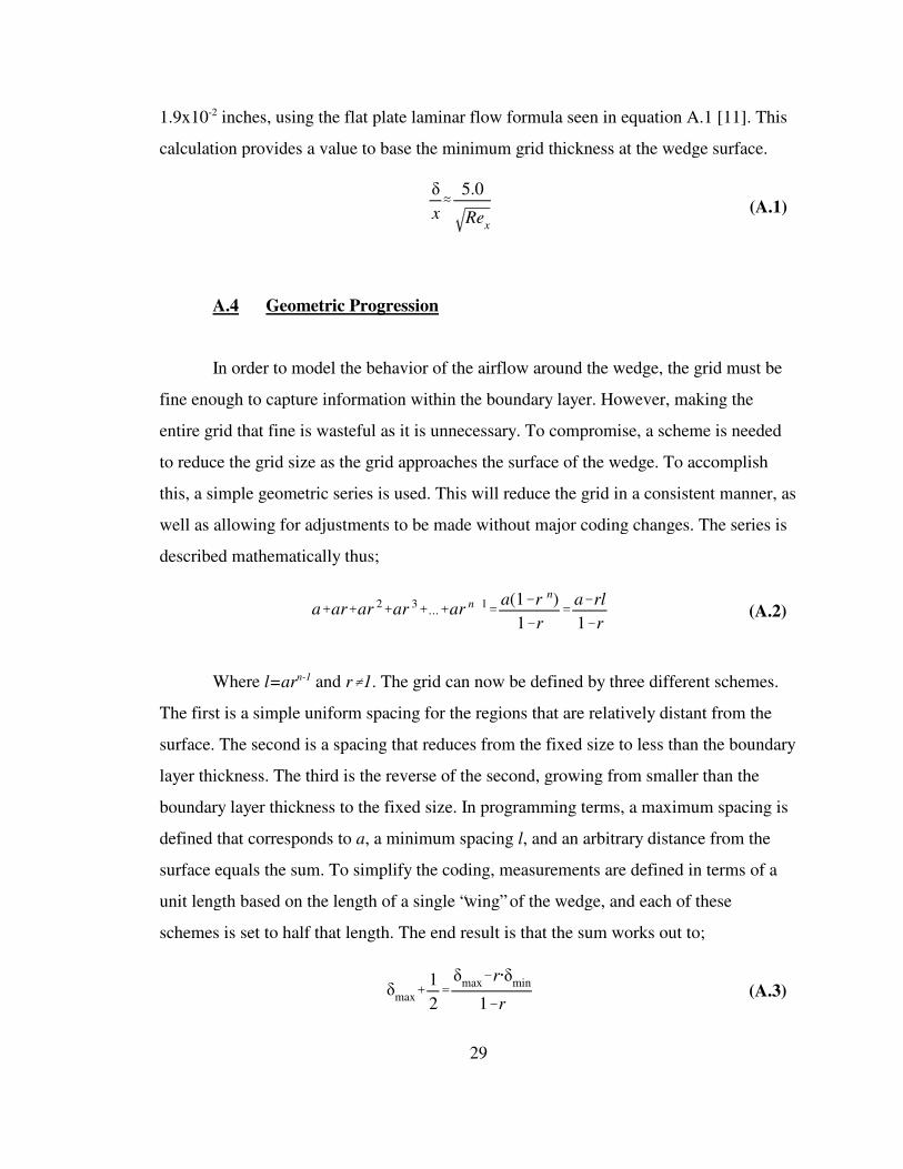
1.9x10 inches, using the flat plate laminar flow formula seen in equation A.1 [11]. This-2
calculation provides a value to base the minimum grid thickness at the wedge surface.
A.4 Geometric Progression
In order to model the behavior of the airflow around the wedge, the grid must be
fine enough to capture information within the boundary layer. However, making the
entire grid that fine is wasteful as it is unnecessary. To compromise, a scheme is needed
to reduce the grid size as the grid approaches the surface of the wedge. To accomplish
this, a simple geometric series is used. This will reduce the grid in a consistent manner, as
well as allowing for adjustments to be made without major coding changes. The series is
described mathematically thus;
Where l=ar and rg1. The grid can now be defined by three different schemes.n-1
The first is a simple uniform spacing for the regions that are relatively distant from the
surface. The second is a spacing that reduces from the fixed size to less than the boundary
layer thickness. The third is the reverse of the second, growing from smaller than the
boundary layer thickness to the fixed size. In programming terms, a maximum spacing is
defined that corresponds to a, a minimum spacing l, and an arbitrary distance from the
surface equals the sum. To simplify the coding, measurements are defined in terms of a
unit length based on the length of a single “wing” of the wedge, and each of these
schemes is set to half that length. The end result is that the sum works out to;
r 11�2/max2/min
30
(A.3)
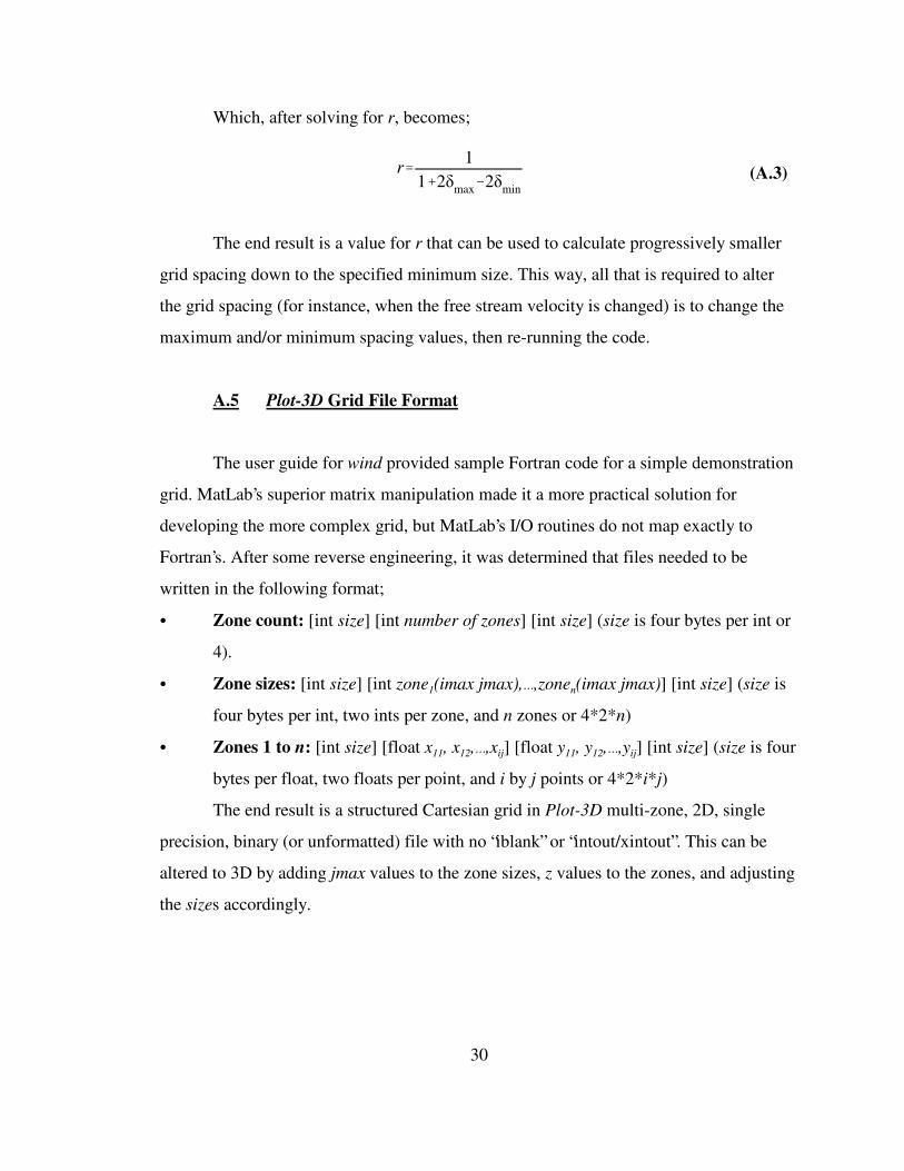
Which, after solving for r, becomes;
The end result is a value for r that can be used to calculate progressively smaller
grid spacing down to the specified minimum size. This way, all that is required to alter
the grid spacing (for instance, when the free stream velocity is changed) is to change the
maximum and/or minimum spacing values, then re-running the code.
A.5 Plot-3D Grid File Format
The user guide for wind provided sample Fortran code for a simple demonstration
grid. MatLab’s superior matrix manipulation made it a more practical solution for
developing the more complex grid, but MatLab’s I/O routines do not map exactly to
Fortran’s. After some reverse engineering, it was determined that files needed to be
written in the following format;
& Zone count: [int size] [int number of zones] [int size] (size is four bytes per int or
4).
& Zone sizes: [int size] [int zone (imax jmax),á,zone (imax jmax)] [int size] (size is1 n
four bytes per int, two ints per zone, and n zones or 4*2*n)
& Zones 1 to n: [int size] [float x , x ,á,x ] [float y , y ,á,y ] [int size] (size is four11 12 ij 11 12 ij
bytes per float, two floats per point, and i by j points or 4*2*i*j)
The end result is a structured Cartesian grid in Plot-3D multi-zone, 2D, single
precision, binary (or unformatted) file with no “iblank” or “intout/xintout”. This can be
altered to 3D by adding jmax values to the zone sizes, z values to the zones, and adjusting
the sizes accordingly.
31
A.6 Other Concerns
The geometry of the wedge is such that the exposed hinge surface “shifts” from
back to front as the wedge angle decreases. In other words, when the wedge is fully
opened (i.e. �=180°), the two flaps form the entire upwind surface, while the hinge is only
exposed in the back, but when the hinge is closed (�=0°), then the leading edge of the
wedge is a half cylinder surface. In order to compensate for this in the grid, it is necessary
to code for the number of points on the front and back of the hinge to vary as the wedge
angle changes.
32
B Sample Code and Parameters
The following samples include the grid generating MatLab “m-file”, as well as
some additional MatLab utilities and REXX scripts.
This study was executed almost entirely on a desktop PC; a 1.3 GHz AMD Duron
processor, 384 MB RAM, running the Red Hat 7.3 distribution of Linux (2.4.18 kernel),
MatLab Student Edition release 12 (MatLab version 6), and ObjectREXX version 2.0.
Wind and its supporting utilities are described in detail in appendix C.
Note: REXX is a very common “procedures” (or “scripting” in *nix parlance)
language on IBM mainframes and is also available in some form on very nearly every PC
operating system. While it is not commonly used on Linux, it is powerful, flexible and
easy to code. The decision to write these utilities in REXX was based on more pragmatic
reasons; the author is fairly fluent in REXX so it was much more expedient to code
utilities with it, rather than spend time learning a more common scripting language.
B.1 Generating the Grid (MatLab m-file)
The following is the MatLab m-file that creates and writes the structured
Cartesian grid.
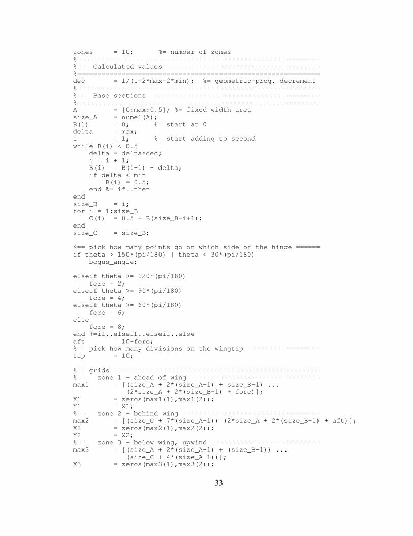
%== 10-zone grid builder, 2-D, V4 =========================%============================================================clc; %== clear the command window%============================================================%== Note to self: =========================================%== MatLab matrix notation is done in R,C format, so x ===%== values correspond to rows and y values columns. ======%============================================================%== "Fixed" values ========================================%============================================================L = 1; %= length (of one butterfly "wing") [inches] %= note: this fixes the units and dimensionst = 0.060; %= thickness of "wing" [unitless]r = 0.125; %= radius of hinge [unitless]theta = 090*(pi/180); %= angle of "wings" [rad]filename = '2d090.grid'; %= for later use...phi = (pi-theta)/2; %= useful angle [rad]beta = pi/2-phi; %= angle on back of hingemax = 0.1; %= largest/ fixed division [unitless]min = 0.001; %= smalllest division [unitless]
33
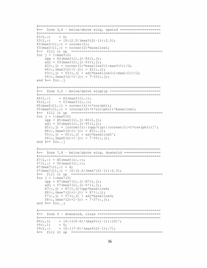
zones = 10; %= number of zones%============================================================%== Calculated values =====================================%============================================================dec = 1/(1+2*max-2*min); %= geometric-prog. decrement%============================================================%== Base sections =========================================%============================================================A = [0:max:0.5]; %= fixed width areasize_A = numel(A);B(1) = 0; %= start at 0delta = max;i = 1; %= start adding to secondwhile B(i) < 0.5 delta = delta*dec; i = i + 1; B(i) = B(i-1) + delta; if delta < min B(i) = 0.5; end %= if..thenendsize_B = i;for i = 1:size_B C(i) = 0.5 - B(size_B-i+1);endsize_C = size_B;
%== pick how many points go on which side of the hinge ======if theta > 150*(pi/180) | theta < 30*(pi/180) bogus_angle;
elseif theta >= 120*(pi/180) fore = 2;elseif theta >= 90*(pi/180) fore = 4;elseif theta >= 60*(pi/180) fore = 6;else fore = 8;end %=if..elseif..elseif..elseaft = 10-fore;%== pick how many divisions on the wingtip ==================tip = 10;
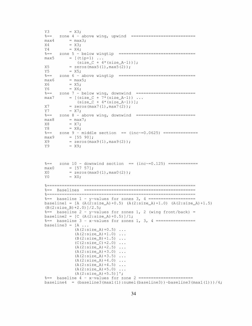
%============================================================%== Baselines =============================================%============================================================%== baseline 1 - y-values for zones 3, 4 ===================baseline1 = [A (A(2:size_A)+0.5) (A(2:size_A)+1.0) (A(2:size_A)+1.5)(B(2:size_B)+2.0)]/2.5;%== baseline 2 - y-values for zones 1, 2 (wing front/back) =baseline2 = [C (A(2:size_A)+0.5)]/1;%== baseline 3 - x-values for zones 1, 3, 4 ================baseline3 = [A ... (A(2:size_A)+0.5) ... (A(2:size_A)+1.0) ... (B(2:size_B)+1.5) ... (C(2:size_C)+2.0) ... (A(2:size_A)+2.5) ... (A(2:size_A)+3.0) ... (A(2:size_A)+3.5) ... (A(2:size_A)+4.0) ... (A(2:size_A)+4.5) ... (A(2:size_A)+5.0) ... (A(2:size_A)+5.5)]';%== baseline 4 - x-values for zone 2 ======================baseline4 = (baseline3(max1(1):numel(baseline3))-baseline3(max1(1)))/4;
35
%== baseline 5 - x-values for zones 5,6 ===================baseline5 = [0:(1/tip):1];%== "origin" - x-y coords for center of rod ===============origin = [2 3.5];%== "corner" - x-y coords for leading wingtip =============corner = [origin(1)-r*cos(phi)+sin(phi) ... origin(2)-r*sin(phi)-cos(phi)];
%============================================================%== Zone 2 - immediately downwind of wing ==================%============================================================X2(max2(1),:) = 6;Y2(max2(1),:) = (2.5:2/(max2(2)-1):4.5);X2(1,1:((max2(2)-aft)/2)) =[-(1-r)*baseline2*sin(phi)+corner(1)+t*cos(phi)];Y2(1,1:((max2(2)-aft)/2)) =[(1-r)*baseline2*cos(phi)+corner(2)+t*sin(phi)];for j = ((max2(2)-aft+2)/2):(max2(2)/2) k = j - (max2(2)-aft+2)/2; alpha = (aft-1-2*k)*beta/(aft-1); X2(1,j) = (origin(1)+r*cos(alpha)); Y2(1,j) = (origin(2)-r*sin(alpha));end %= for..j%== fill it up =============================================for j = 1:(max2(2)/2) opp = X2(max2(1),j)-X2(1,j); adj = Y2(max2(1),j)-Y2(1,j); hyp = sqrt(opp^2+adj^2); X2(1:max2(1),j) = X2(1,j) + opp*baseline4; X2(1:max2(1),(max2(2)+1-j)) = X2(1:max2(1),j); Y2(1:max2(1),j) = Y2(1,j) + adj*baseline4; Y2(1:max2(1),(max2(2)+1-j)) = 7-Y2(1:max2(1),j);end %== for..j
36
%============================================================%== Zone 3,4 - below/above wing, upwind ====================%============================================================X3(1,:) = 0;Y3(1,:) = [0:(2.5/(max3(2)-1)):2.5];X3(max3(1),:) = corner(1);Y3(max3(1),:) = corner(2)*baseline1;%== fill it up =============================================for j = 1:max3(2) opp = X3(max3(1),j)-X3(1,j); adj = Y3(max3(1),j)-Y3(1,j); X3(:,j) = corner(1)*baseline3(1:max3(1))/2; X4(:,(max3(2)+1-j)) = X3(:,j); Y3(:,j) = Y3(1,j) + adj*baseline3(1:max1(1))/2; Y4(:,(max3(2)+1-j)) = 7-Y3(:,j);end %== for..j
%============================================================%== Zone 5,6 - below/above wingtip =========================%============================================================X5(1,:) = X3(max3(1),:);Y5(1,:) = Y3(max3(1),:);X5(max5(1),:) = corner(1)+t*cos(phi);Y5(max5(1),:) = (corner(2)+t*sin(phi))*baseline1;%== fill it up =============================================for j = 1:max5(2) opp = X5(max5(1),j)-X5(1,j); adj = Y5(max5(1),j)-Y5(1,j); X5(:,j) = [corner(1):(opp/tip):(corner(1)+t*cos(phi))]'; X6(:,(max5(2)+1-j)) = X5(:,j); Y5(:,j) = Y5(1,j) + adj*baseline5'; Y6(:,(max5(2)+1-j)) = 7-Y5(:,j);end %== for..j
%============================================================%== Zone 7,8 - below/above wing, downwind ==================%============================================================X7(1,:) = X5(max5(1),:);Y7(1,:) = Y5(max5(1),:);X7(max7(1),:) = 6;Y7(max7(1),:) = [0:(2.5/(max7(2)-1)):2.5];%== fill it up =============================================for j = 1:max7(2) opp = X7(max7(1),j)-X7(1,j); adj = Y7(max7(1),j)-Y7(1,j); X7(:,j) = X7(1,j)+opp*baseline4; X8(:,(max7(2)+1-j)) = X7(:,j); Y7(:,j) = Y7(1,j) + adj*baseline4; Y8(:,(max7(2)+1-j)) = 7-Y7(:,j);end %== for..j
%============================================================%== Zone 9 - downwind, close ===============================%============================================================X9(:,1) = [6:((10-6)/(max9(1)-1)):10]';Y9(:,1) = 0;Y9(1,:) = [0:((7-0)/(max9(2)-1)):7];%== fill it up =============================================
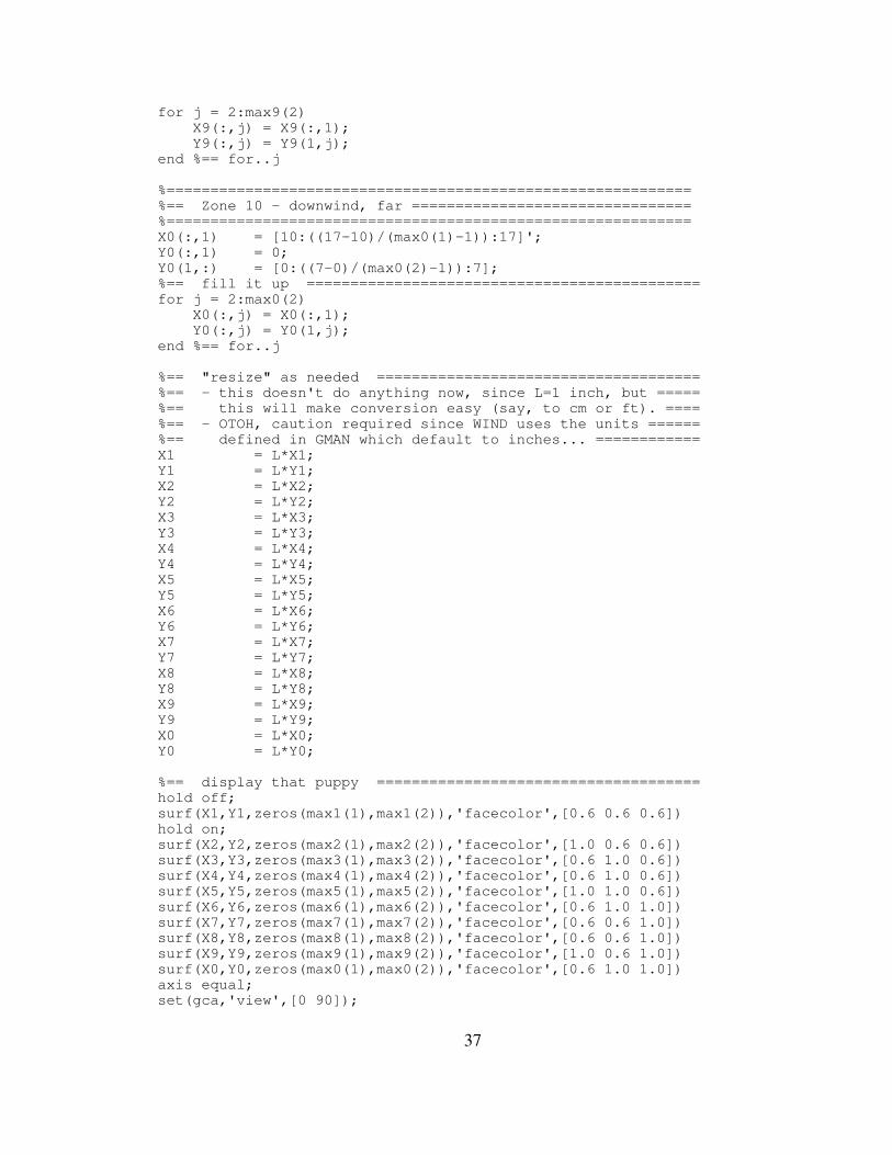
%============================================================%== Zone 10 - downwind, far ================================%============================================================X0(:,1) = [10:((17-10)/(max0(1)-1)):17]';Y0(:,1) = 0;Y0(1,:) = [0:((7-0)/(max0(2)-1)):7];%== fill it up =============================================for j = 2:max0(2) X0(:,j) = X0(:,1); Y0(:,j) = Y0(1,j);end %== for..j
%== "resize" as needed =====================================%== - this doesn't do anything now, since L=1 inch, but =====%== this will make conversion easy (say, to cm or ft). ====%== - OTOH, caution required since WIND uses the units ======%== defined in GMAN which default to inches... ============X1 = L*X1;Y1 = L*Y1;X2 = L*X2;Y2 = L*Y2;X3 = L*X3;Y3 = L*Y3;X4 = L*X4;Y4 = L*Y4;X5 = L*X5;Y5 = L*Y5;X6 = L*X6;Y6 = L*Y6;X7 = L*X7;Y7 = L*Y7;X8 = L*X8;Y8 = L*Y8;X9 = L*X9;Y9 = L*Y9;X0 = L*X0;Y0 = L*Y0;
The first line(s) is a freeform title that is included in later output files. The “/”
character indicates a comment. The “freestream” keyword is followed by “static” or
“total”, then the Mach number of the freestream, the pressure (in psi), the temperature (in
degrees Rankine), the angle of attack and then angle of yaw (in degrees). For these
conditions, the Mach number of 0.125 translates to 42.5 m/s which is slightly higher than
the maximum sustainable velocity of 42 m/s managed in the Eddy study’s wind tunnel.
The “turbulence” keyword is followed by one of nine different turbulence models
available in wind. In this case, the SST (Shear Stress Transport) two equation model was
selected as most appropriate for the calculations being done (see section 3.3). The
“cycles” keyword is used to specify the number of 5-iteration cycles to run. Selecting 20
cycles and running multiple times allowed the automation of “snapshots” of the solution
as it developed.
40
B.3 Running Wind Multiple Times (REXX script)
In order to capture data as the solution evolved, it was necessary to run wind
multiple times, stopping in between to “snapshot” the results. Wind is designed to default
to continuing where it left off when interrupted, making this a straightforward set up. The
parameters (see B.2) were set to 100 iterations (20 five-iteration cycles) to allow a
reasonable number of calculations between each stop.
#!/usr/bin/rexx/* run_many.cmd - REXX exec to execute WIND multiple times **********/trace 'O'
/* read in the filename for .dat, .lis, .cfl files ******************//* note: file_names ARE case sensitive. use "parse arg" instead... **/parse arg angle suffix .if \datatype(angle,'N') then do /* angle is not numeric; use default */ file_name = '2d120' grid_name = '2d120'end /* if..then..do */else do angle = right(angle,3,'0') /* force zero-padding, 3 digits ****/ file_name = '2d'angle||suffix grid_name = '2d'angleend /* else..do */
/* copy the grid file for use with CFPOST ***************************/"cp" grid_name".cgd temp.cgd"
say "Executing wind for input file" file_name".dat"
/* 5 iterations per cycle, 20 cycles per run = 10000 iterations. ****/do i = 1 to 100 fu = i-1 /* just a "before" variable ******************************/ say "=============== Iteration" fu"01 to" i"00 =============" time() "wind -runinplace", /* force to run locally ******************/ "-runque REAL", /* run in the "real" queue ***************/ "-dat" file_name, /* specify the dat file ******************/ "-list" file_name, "-grid" grid_name, "-flow" file_name, "-program wind5", /* specify which version to run ***********/ "-batch", /* force batch (no prompting) *************/ "-nobg" /* force foreground ***********************/
/* Theoretically, rc is set to the exit return code from the */ /* command issued. However, a bad grid file during a test run */ /* demonstrated that WIND (or perhaps Linux commands in general) */ /* does not set the rc properly; use "tail -f <filename.lis> to */ /* ensure that things are running correctly... ********************/ if rc = 0 then do /* set up the flow-file for use with CFPOST *********************/ "cp" file_name".cfl temp.cfl"
41
"cfpost < mkplot.jou >" file_name"."right(i,3,'0')".log" "cp temp.q" file_name"."right(i,3,'0')".q" "cp" file_name".cfl" file_name"."right(i,3,'0')".cfl" end /* if..then..do */ else do say "** failed around" i"00 iterations with rc="rc leave end /* else..do */end /* do..i */
exit
B.4 Pressure and Velocity Data Extraction (REXX script)
The cfpost utility provides the facility to extract different data from the “common
flow file” generated by wind. With the right supporting software (e.g. Visual3), this data
can be displayed directly from cfpost. As an alternative, data can be extracted as space-
delimited text for processing less directly; this utility executes a script in cfpost that does
just that, for each “snapshot” taken during the wind run.
#!/usr/bin/rexx/* smee.cmd - REXX kludge to generate output for "clean_list.cmd" */trace 'O'
/* read in the filename for .dat, .lis, .cfl files ******************//* note: file_names ARE case sensitive. use "parse arg" instead... **/parse arg angle suffix .if \datatype(angle,'N') then do /* if angle is not numeric, default */ file_name = '2d120' grid_name = '2d120'end /* if..then..do */else do angle = right(angle,3,'0') /* force zero-padding, 3 digits ****/ file_name = '2d'angle||suffix grid_name = '2d'angleend /* else..do */
/* copy the grid file for use with CFPOST ***************************/"cp" grid_name".cgd temp.cgd"
/* set up the flow-file for use with CFPOST *************************/do i = 1 to 100 "cp" file_name"."right(i,3,'0')".cfl temp.cfl" "cfpost < p_plot.jou > p_plot.log" "cfpost < v_plot.jou > v_plot.log" "clean_list.cmd >"file_name"."right(i,3,'0')".csv"end /* do..i */
exit
42
B.5 Clean-up Cfpost Output (REXX script)
The output from the previous step is not easily readable with any of MatLab’s
standard routines, so another utility was written to strip headers and extra spaces from the
output and add commas between values. This allows the results to be read directly in to
MatLab with a CSVREAD (Comma Separated Values read) routine.
#!/usr/bin/rexx/* REXX exec to clean up output from CFPOST *************************/trace 'N'
/* set a signal ("goto") to close files after interupt **************/signal on halt
/* identify files with pressure and velocity values *****************/file1 = "p_temp.lis"file2 = "v_temp.lis"
/* open output files from CFPOST ************************************/void = stream(file1,"C","OPEN")void = stream(file2,"C","OPEN")curzone = 0
/* read through the output files which should be the same length...**/do while lines(file1) > 0 /* parse around the "ZONE" header: if it's there, then get the **/ /* zone dimensions, otherwise build the output string which will **/ /* include i, j, k, x, y, p. p0, v, u, V and W ********************/ parse upper value linein(file1) with before "ZONE" after . parse upper value linein(file2) with . . . v_data if datatype(after,"N") then do /* ignore non-numeric "zones" ******/ if after > 0 & curzone \= after then do if curzone > 0 then call write_zone else nop curzone = after big_i = 0 big_j = 0 big_k = 0 end /* if..do */ else nop end /* if..do */ else do /* "ZONE" not found, but is it data or header? ************/ parse var before i j k p_data if \datatype(i,"N") then /* if i is not numeric, then skip it ***/ iterate else do /* step up the max i, j, k values to find dimensions ****/ if big_i < i then big_i = i
43
if big_j < j then big_j = j if big_k < k then big_k = k /* it's a data line: parse out the desired values *************/ parse var p_data x y p p0 . p_data = x','y','p','p0 /* we need commas for CSVREAD to work */ parse var v_data u v big_V big_W . v_data = u','v','big_V','big_W queue i','j','k','p_data','v_data /* "stack" the output rec ***/ end /* else..do */ end /* else..do */end /* do..while */
call write_zone /* the very last zone is still in the stack *********/
/* interupted or finished; close the input files ********************/halt:void = stream(file1,"C","CLOSE")void = stream(file2,"C","CLOSE")
exit
write_zone: /********************************************************//*********** *//* this subroutine pulls a single zone's info off the stack and *//* writes it to STDOUT. When everything works, just use the ">" *//* redirection operator to pipe the output to a file... *//********************************************************************/ say big_i','big_j','big_k /* write the zone dimensions ************/ do queued() pull stuff say stuff end /* do..queued() */return
B.6 Displaying “Surfaces” (MatLab m-file)
The previous two utilities result in a file with data (static and total pressure,
velocity in x and y and an average, and vorticity in this case, though other data can be
extracted) in an array that can be read into arrays for each zone and then displayed with
the following code and, optionally, saved in different formats. There is a lot of
redundancy in the code, but the arrays vary in size from zone to zone, and zones 1 and 2
vary in size for different wedge angles.
%== Kludge to show pressure "surfaces" ================================%===+====1====+====2====+====3====+====4====+====5====+====6====+====7clc;
Figure D.1.2 Convergence data for Shear Stress Transportcalculations, 30° wedge run.
D.1 Solution and Convergence, 30° Wedge
Figure D.1.1 Convergence data for Navier-Stokes calculations forthe 30° wedge run.
55
Figure D.1.3 Total pressure values for 30° wedge after 10,000iterations.
Figure D.1.4 Average velocity values for 30° wedge after 10,000iterations.
4 4.5 5 5.5 6 6.5 7 7.5 80
0.5
1
1.5
CP vs. position, 30 Wedge
Vertical Position [in]
CP [%
]
Meas.Calc.
56
Figure D.1.5 Comparison of pressure coefficient data for 30° wedge.Values were measured at slot two (three inches downwind of the wedge)in the Eddy study and computed by wind. The calculated values are theaverage of three thousand iterations, normalized to the largest measuredvalue of C due to the lack of measured maximum pressure data.p
2D, 60 degree flap, SST, M=0.125
Zone 1 Zone 2Zone 3 Zone 4Zone 5 Zone 6Zone 7 Zone 8Zone 9 Zone 10
Figure D.2.2 Convergence data for Shear Stress Transportcalculations, 60° wedge run.
D.2 Solution and Convergence, 60° Wedge
Figure D.2.1 Convergence data for Navier-Stokes calculations forthe 60° wedge run.
58
Figure D.2.3 Total pressure values for 60° wedge after 10,000iterations.
Figure D.2.4 Average velocity values for 60° wedge after 10,000iterations.
4 4.5 5 5.5 6 6.5 7 7.5 80
0.5
1
1.5
CP vs. position, 60 Wedge
Vertical Position [in]
CP [%
]
Meas.Calc.
59
Figure D.2.5 Comparison of pressure coefficient data for 60° wedge.Values were measured at slot two (three inches downwind of the wedge)in the Eddy study and computed by wind. The calculated values are theaverage of three thousand iterations, normalized to the largest measuredvalue of C due to the lack of measured maximum pressure data.p
2D, 90 degree flap, SST, M=0.125
Zone 1 Zone 2Zone 3 Zone 4Zone 5 Zone 6Zone 7 Zone 8Zone 9 Zone 10
Figure D.3.2 Convergence data for Shear Stress Transportcalculations, 90° wedge run.
D.3 Solution and Convergence, 90° Wedge
Figure D.3.1 Convergence data for Navier-Stokes calculations forthe 90° wedge run.
61
Figure D.3.3 Total pressure values for 90° wedge after 10,000iterations.
Figure D.3.4 Average velocity values for 90° wedge after 10,000iterations.
4 4.5 5 5.5 6 6.5 7 7.5 80
0.5
1
1.5C
P vs. position, 90 Wedge, slot 2
Vertical Position [in]
CP [%
]
Meas.Calc.
62
Figure D.3.5 Comparison of pressure coefficient data for 90° wedge.Values were measured at slot two (three inches downwind of the wedge)in the Eddy study and computed by wind. The calculated values are theaverage of three thousand iterations, normalized to the largest measuredvalue of C due to the lack of measured maximum pressure data.p
2D, 120 degree flap, SST, M=0.125
Zone 1 Zone 2Zone 3 Zone 4Zone 5 Zone 6Zone 7 Zone 8Zone 9 Zone 10
Figure D.4.2 Convergence data for Shear Stress Transportcalculations, 120° wedge run.
D.4 Solution and Convergence, 120° Wedge
Figure D.4.1 Convergence data for Navier-Stokes calculations forthe 120° wedge run.
64
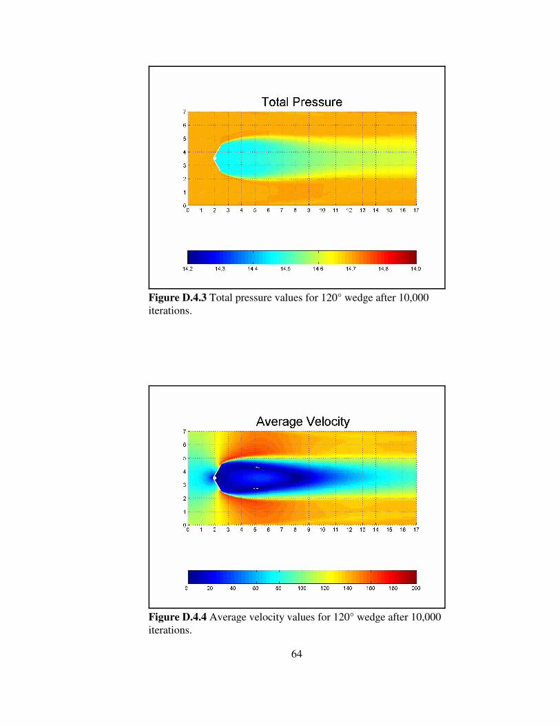
Figure D.4.3 Total pressure values for 120° wedge after 10,000iterations.
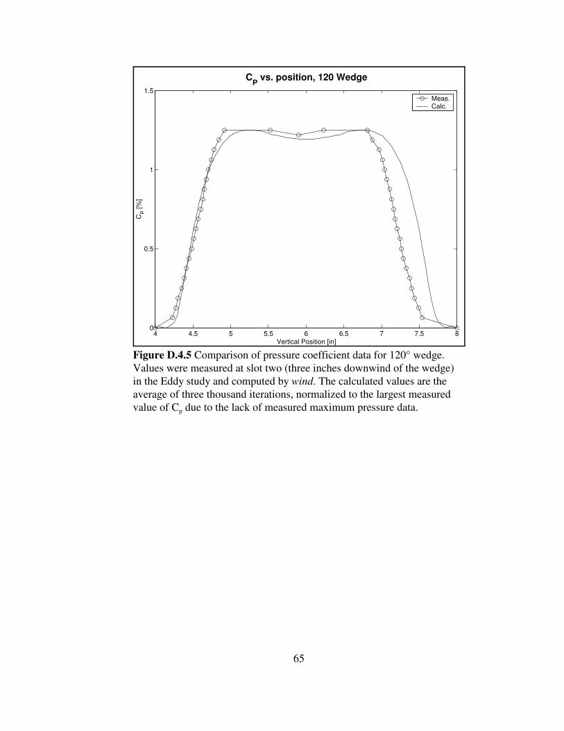
Figure D.4.4 Average velocity values for 120° wedge after 10,000iterations.
4 4.5 5 5.5 6 6.5 7 7.5 80
0.5
1
1.5
CP vs. position, 120 Wedge
Vertical Position [in]
CP [%
]
Meas.Calc.
65
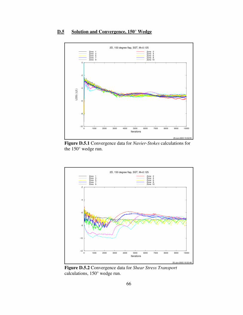
Figure D.4.5 Comparison of pressure coefficient data for 120° wedge.Values were measured at slot two (three inches downwind of the wedge)in the Eddy study and computed by wind. The calculated values are theaverage of three thousand iterations, normalized to the largest measuredvalue of C due to the lack of measured maximum pressure data.p
2D, 150 degree flap, SST, M=0.125
Zone 1 Zone 2Zone 3 Zone 4Zone 5 Zone 6Zone 7 Zone 8Zone 9 Zone 10
Figure D.5.2 Convergence data for Shear Stress Transportcalculations, 150° wedge run.
D.5 Solution and Convergence, 150° Wedge
Figure D.5.1 Convergence data for Navier-Stokes calculations forthe 150° wedge run.
67
Figure D.5.3 Total pressure values for 150° wedge after 10,000iterations.
Figure D.5.4 Average velocity values for 150° wedge after 10,000iterations.
4 4.5 5 5.5 6 6.5 7 7.5 80
0.5
1
1.5
CP vs. position, 150 Wedge
Vertical Position [in]
CP [%
]
Meas.Calc.
68
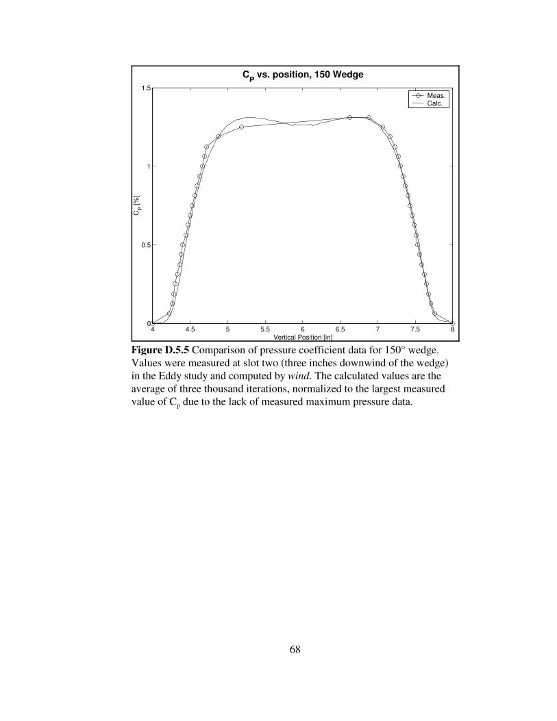
Figure D.5.5 Comparison of pressure coefficient data for 150° wedge.Values were measured at slot two (three inches downwind of the wedge)in the Eddy study and computed by wind. The calculated values are theaverage of three thousand iterations, normalized to the largest measuredvalue of C due to the lack of measured maximum pressure data.p
69
Vita
Keith P Savage was born in Williams Air Force Base, Arizona, in 1961. Raised on
Air Force bases, he settled down in Colorado after graduating high school. After spending
sixteen years working on mainframe computers, he went back to school, receiving his
B.S. in Metallurgical and Materials Engineering from Colorado School of Mines in 2001.
He is currently pursuing an M.S. in Aerospace Engineering at the University of Tennessee