CFD-simulations of urea-SNCR for NO x -reduction in flue gases from biomass combustion Master’s thesis in Sustainable Energy Systems NING GUO Department of Applied Mechanics CHALMERS UNIVERSITY OF TECHNOLOGY G¨ oteborg, Sweden 2015
Transcript
CFD-simulations of urea-SNCR forNOx-reduction in flue gases from biomasscombustionMaster’s thesis in Sustainable Energy Systems
NING GUO
Department of Applied MechanicsCHALMERS UNIVERSITY OF TECHNOLOGYGoteborg, Sweden 2015
MASTER’S THESIS IN SUSTAINABLE ENERGY SYSTEMS
CFD-simulations of urea-SNCR for NOx-reduction in flue gases from biomasscombustion
NING GUO
Department of Applied MechanicsDivision of Fluid Dynamics
CHALMERS UNIVERSITY OF TECHNOLOGY
Goteborg, Sweden 2015
CFD-simulations of urea-SNCR for NOx-reduction in flue gases from biomass combustionNING GUO
Master’s thesis 2015:42ISSN 1652-8557Department of Applied MechanicsDivision of Fluid DynamicsChalmers University of TechnologySE-412 96 GoteborgSwedenTelephone: +46 (0)31-772 1000
Chalmers ReproserviceGoteborg, Sweden 2015
CFD-simulations of urea-SNCR for NOx-reduction in flue gases from biomass combustionMaster’s thesis in Sustainable Energy SystemsNING GUODepartment of Applied MechanicsDivision of Fluid DynamicsChalmers University of Technology
Abstract
Urea-SNCR is a technology that can reduce NOx emissions from biomass combustion. In order to havegood results of NOx reduction in a certain urea-SNCR system, simulations are advised to be conducted, itcan be used to optimize the system design, which also significantly reduces the time and costs of experimentaloptimization in the real plant
In the simulation, urea evaporation and decomposition and NOx reduction are two important processesthat needs to be simulated. In this thesis work, a CFD model (k − ε model, chemical-turbulence interactionmodel and discrete random walk model) is used to simulate the urea evaporation and decomposition. A CSTR(Continuous Stirred-Tank Reactor) model, a PFR (Plugged Flow Reactor) model and the CFD model are allevaluated in simulations of the NOx reduction process.
The CSTR, PFR, and CFD models are tested at different conditions (temperature, geometry, retention time,injection points, etc.) for a complete urea-SNCR process. Under the given conditions, the effects of turbulentvelocity fluctuations on the urea spray, the effects of mixing and chemical kinetics on each reaction, the effectsof temperature and retention time on the NOx reduction and the reaction selectivities are studied. Then theCFD model is validated against experimental data from a power plant in Rorvik, which shows the CFD modelis suitable for the simulation. Based on the CFD simulations, a new injection strategy for urea-water mixtureis evaluated.
Keywords: urea-SNCR, CSTR, PFR, CFD
Acknowledgements
I would like to express my gratitude for finishing my master’s thesis.Firstly, I greatly thank my supervisor Assistant Professor Henrik Strom for his great knowledge, guidance
and patience. Without him, this work could not reach the level it is now.I would also like to give credits to Oskar Finnermann for his contribution in CSTR, PFR and CFD simulations
and report proof reading. Narges Razmjoo, Michael Strand and Jan Brandin from Linnaeus University providedexperimental data and insightful input, which is appreciated.
Professor Srdjan Sasic is kind enough to act as my examiner. Special thanks to everyone at the Division ofFluid Dynamics at Chalmers for a friendly working environment and nice coffee breaks.
This master thesis is partly funded by Chalmers Avencez Scholarship.
One way to reduce CO2 emissions from the energy production industry is to produce sustainable energy byusing biomass combustion boilers. However, part of the nitrogen in the biomass fuel and air is converted tonitrogen oxides (NOx ), which is harmful to the environment and public health [1]. To solve this problem, onepossibility is to use urea to react with the exhaust gases from combustion so that NOx can be converted tonitrogen (N2). In other words, ammonia (NH3) can be produced from urea decomposition and then reduceNOx to N2. Urea-SNCR (selective non-catalytic reduction) technology is one feasible way to do it.
In the industries, in order to save time and money, simulations are often conducted before experimentsare carried out. Numerical simulations, when carefully executed, have the potential to reduce the time fromprototype to final solution by orders of magnitude. In these cases, model selections are crucial. A simplifiedmodel is computationally cheap, but may be far away for the reality. A complicated model is close to the realpractice but maybe too computationally expensive.
The Urea-SNCR process can be divided into two parts (sub-processes): 1) urea evaporation and decompo-sition, in which urea-water mixture is injected to the flue gases from biomass combustion, decomposes andproduces NH3; 2) NOx reduction, in which NH3 reduces NO into N2. Different models must be chosen tosimulate each aspect of each sub-process. Different combinations of models affect the simulation results andthe computational resources required.
In this master thesis, a Continuous Stirred-Tank Reactor (CSTR) model, a Plug Flow Reactor (PFR) modeland a Computational Fluid Dynamics (CFD) model are used to simulate the urea-SNCR process. Comparingwith experimental data from a Rorvik power plant, a guideline of model selection has been proposed. A newinjection strategy for this power plant is also tested in the simulation.
Besides model selection, the impact of turbulent velocity fluctuations on the convective heat transfer ureadroplets is also studied.
However, the biomass combustion process before the urea-SNCR system will not be studied in this thesis.
1
2 Theory
In this chapter, the theoretical background of the urea SNCR process and the models that are used to simulatethis process are explained.
2.1 Urea SNCR process
The urea SNCR process can be divided into two parts: 1) urea evaporation and decomposition, and 2) NOx
reduction.
2.1.1 Urea evaporation and decomposition
First of all, urea-water mixture droplets, whose temperature is relatively low, are injected into biomasscombustion flue gases, whose temperature is relatively high. Due to the temperature difference, urea-waterparticles are heated and vaporize to water vapor and urea vapor. The evaporation process can therefore bemodeled as two parallel evaporation fluxes.
In the CFD simulations, the convection/diffusion controlled model is used for mass transportation [2][3]:
dmi
dt= Apkc,iρ∞ln (1 +Bi,m) (2.1)
where m is the mass, t is the time, kc is the mass transfer coefficient, Ap is the droplet surface area, ρ∞ is thedensity of bulk gas, Mw is the molecular weight, Bm is the Spalding mass number and subscript i denotes thespecies component i.
The heat balance is defined as
mpCpdTpdt
= hAp (T∞ − Tp) +∑i
dmi
dt(hvap,i) (2.2)
where Cp is the heat capacity of the particle, Tp is the particle temperature, h is the heat transfer coefficientfor the convective/diffusion controlled model, T∞ is the local temperature of continuous phase, dmi
dt is from Eq.(2.1), hvap is the latent heat of vaporization.
According the work of Lundstrom et al. [4], the relationship of urea vapor pressure, purea [Pa], andtemperature, T [K] (within the range of 406K-550K) is simulated as in (2.3):
log10 purea(T ) = A− B
C + T(2.3)
where A, B and C are constants as stated in Table 2.1.
Constant A B CValue 1.1663E+01 4.0854E+03 3.3953E-3
Table 2.1: Antoine constants for urea vapor pressure and temperature (406K-550K)
In this work, the water vapor pressure is modelled using piecewise-linear method as in Table 2.2 accordingto the Fluent database.
Table 2.2: Saturation pressure [Pa] and temperature [K] of water vapor
2
Then the urea vapor starts to break down, as seen in Reaction {2.1} and {2.2}, these chemical reactions arechosen based on the work of Østberg et al. [5]. The reaction rate parameters are listed in Table 2.3.
CO(NH2)2→ NH3 + HNCO {2.1}
CO(NH2)2 + H2O → 2NH3 + CO2 {2.2}
In Table 2.3, A is the pre-exponent factor in m-mol-s, b is the temperature exponent and E is the activation
Reaction A b E{2.1} 1.27E+04 0 65048.109{2.2} 6.13E+04 0 87819.133
Table 2.3: Simplified chemical process of urea breakdown
energy in J/mol.In Reaction {2.1}, only half of the N in CO(NH2)2 is converted to NH3 while all of the N in CO(NH2)2 is
converted to NH3 in Reaction {2.2}.
2.1.2 NOx reduction
In the NOx reduction process, NH3, produced in the urea breakdown, can reduce NO, produced from biomasscombustion, to N2. But NH3 can also be oxidized by O2 into NO. As seen in Reaction {2.3}, {2.4} and Table2.4, the reaction rates are calculated based on the work of Rota et al. [6]. The variables and units in Table 2.4and 2.3 are consistent.
{2.3}NO + NH3 + 1/4O2 → N2 + 3/2H2O
NH3 + 5/4O2 → NO + 3/2H2O {2.4}
Reaction A b E{2.3} 4.24E+02 5.30 349937.06{2.4} 3.50E-01 7.65 524487.005
Table 2.4: Simplified chemical process of NOx reduction
2.2 Simulation models
There are several different reactor models that are used industrially to simulate the urea SNCR process. Thesemodels are based on different assumptions regarding the flow field (and thus the mixing) in the urea SNCRsystem. In this work, these different models are considered: the CSTR model, the PFR model and a full CFDset up.
2.2.1 CSTR model
According to Roberts et al. [7], the ideal Continuous Stirred-Tank Reactor (CSTR) model is characterized byperfect mixing, which means it assumes that the temperature and concentration are uniform in the reactor.
The conservation equation of mass for a given species in a CSTR reads:
dρYiV
dt= [uAρYi]in − [uAρYi]out − ri (2.4)
where ρ is density, Y is mass fraction, V is volume, t is time, u is velocity, A is the cross-sectional area, r isthe net reaction rate and subscript i means different species, in and out represent the inlet and the outletrespectively. Each term in Eq. (2.4) is accumulation term, incoming convective term, outgoing convective termand source term respectively.
3
Since N2 makes up the majority of the flue gases and the molar differences between reactants and productsin Reaction {2.3} and {2.4} is not large, it is assumed equimolarity in the CSTR model in this thesis work,which reduces Eq. (2.4) into
VdCidt
= uA (Ci,in − Ci)− ri (2.5)
where C is the molar concentration. Since the average residence time is
τ =V
uA(2.6)
Eq. (2.5) now is converted todCidt
=Ci,in − Ci
τ− ri (2.7)
It is assumed to be steady state, so
0 =Ci,in − Ci
τ− ri (2.8)
Eq. (2.8) is the base of the Matlab simulation of CSTR model.
2.2.2 PFR model
In a plug flow reactor (PFR) model [7], the most common one-dimensional reactor model, it is often assumedthat:
1. In the axial direction (flow direction), there is no mixing (no diffusion);
2. The properties in the flow perpendicular direction are uniform;
In this thesis work, it is also assumed that:
1. The temperature is constant;
2. The state is steady;
3. The ideal gas law applies.
The differential conservation of species for a PFR reads
ρ∂Yi∂t
= −ρ∂ (uYi)
∂x+m′′′ (2.9)
where the terms represent an accumulation term, a convective transportation term and a source term respectively.Since it is steady state Eq. (2.9) is converted into
ρ∂ (uYi)
∂x= m′′′ (2.10)
Similar to the CSTR model, assuming equimolarity, Eq. (2.10) can be rewritten to
udCidx
= ri (2.11)
and this is base of the Matlab simulation of PFR model.
2.2.3 CFD model
For incompressible flow the continuity equation reads [8]
∂Uj∂xj
= 0 (2.12)
and the Navier-Stokes equation reads [8]
∂Ui∂t
+ Uj∂Ui∂xj
= −1
ρ
∂P
∂xi+ ν
∂2Ui∂xj∂xj
(2.13)
4
In Reynolds decomposition [9], an instantaneous variable can be divided into a mean part and a fluctuatingpart. Take velocity as an example:
~U = ~U + u (2.14)
Instantaneous velocity = Mean velocity + Fluctuating velocity
therefore, the Eq. (2.12) can be rewritten as∂Ui∂xi
= 0 (2.15)
and (2.13) can be rewritten as
∂Ui∂t
= Uj∂Ui∂xj
= −1
ρ
∂
∂xj
[Pδij + µ
(∂Ui∂xj
+∂Uj∂xi
)− ρuiuj
](2.16)
Eq (2.15) and (2.16) are the RANS (Reynolds Averaged Navier-Strokes) equations.The k − ε model, based on RANS, is one of the most frequently used turbulence model in CFD simulations.
The standard k-ε model is used here and the transport equations for k and ε are [10][9]:
∂ρk
∂t+ div(ρk~U) = div[
µtσk
gradk] + 2µtSij · Sij − ρε (2.17)
∂ρε
∂t+ div(ρε~U) = div[
µtσε
gradk] + C1εε
k2µtSij · Sij − C2ερ
ε2
k(2.18)
where the eddy viscosity is
µt = ρCuk2
ε(2.19)
The Eq. (2.17), (2.18) and (2.19) have 5 adjustable constants as listed in Table 2.5.
Constant Cµ σk σε C1ε C2ε
Value 0.09 1.00 1.30 1.44 1.92
Table 2.5: Constants for the standard k − ε model
The standard wall function [10] is used to describe the near wall region.
2.2.4 Chemical-turbulence interaction model
Chemical reactions occur at the molecular level. The reacting molecules have to meet (a process governedby mixing) before they can react (a process governed by chemical kinetics). So it is great of importance todetermine whether the mixing rate and/or the chemical kinetics is the limiting factor in the overall reactionrates in reactive turbulent flows.
The Dahmkohler number is a dimensionless number that describes the relative importance of mixing andkinetics in a turbulent reactive flow. It is defined as [8]:
Da =Typical time required for mixing
Typical time required for chemical reactions(2.20)
If Da� 1, chemical kinetics are slow comparing to the mixing rate. If Da� 1, it is the other way around.But when Da ≈ 1, the chemical kinetics and mixing rate are in the same order of magnitude.
If only chemical kinetics is of interest, reaction rates can be determined by Arrhenius kinetic expressions[11][12] as in Eq. (2.21) while turbulence mixing is ignored.
k = Ae−EaRT (2.21)
In Eq. (2.21), k [mol · m−3 · s−1] is the rate constant of a chemical reaction, T [K] is the temperature, A[K-mol-m3] is the pre-exponential factor, Ea [J/mol] is the activation energy and R [J · K−1 ·mol−1] is theuniversal gas constant. The approach is known as the Laminar Finite Reaction model, based on the workof Magnussen et al. [13], avoids calculating Arrhenius kinetics by assuming that the reactions are entirely
5
controlled by turbulent mixing. In this model, the net production rate of species i due to reaction r is given bythe smaller value of (2.22) and (2.23)
Ri,r = ν′
i,rMw,iAρε
kminR
(YR
ν′R,rMw,R
) (2.22)
Ri,r = ν′
i,rMw,iABρε
k
∑P YP∑N
j ν′′j,rMw,j
(2.23)
where Y is the mass fraction, A = 4.0 and B = 0.5 are empirical constants, subscript P is any product speciesand R is a particular reactant.
In Ansys Fluent, the so called finite reaction/eddy-dissipation model uses the limiting factor (the mixingrate and/or the chemical kinetics) to determine the local, transient reaction rate.
2.2.5 Euler-Lagrange model and discrete random walk model
The Euler-Lagrange model is one of the most frequently used models for disperse multiphase flows when theparticle volume loading is low so the effects of particles on the fluid and other particles can be treated witheither one-way or two-way coupling. In the Euler-Language model, the fluid phase is treated as a continuumand can be modelled by using standard RANS models (for example, the standard k − ε model), and the effectsof the dispersed phase (the droplets) are represented by source terms in the continuous phase balance equations.Each particle (or each bundle of particles) is tracked and its trajectory is calculated from Newton’s second lawof motion [8].
where md is the particle mass, Ui,d is the particle linear velocity, Fi,Darg is the drag force, Fi,Press is thepressure force due to pressure gradient, Fi,V irt is the virtual mass force due to acceleration of surroundingfluid, Fi,History is the history force due to changes in boundary layer, Fi,Lift is the Saffman and Magnus liftforce due to velocity gradient and particle rotation, Fi,Therm is the thermophoretic force due to a temperaturegradient, Fi,Turb is the force due to turbulent fluctuations and Fi,Brown is the Brownian force due to molecularcollisions. In this thesis work, only Fi,Darg and Fi,Bouy are considered. Turbulent fluctuations are not modelledas a force, but as a variation of the continuous phase velocity seen by the droplets.
Since the dispersed phase is being tracked in a RANS flow field, a method must be used by which theparticles are made to interact also with the turbulent fluctuations. In the work of Gosman et al. [14], an EddyInteraction model is developed to describle particle dispersion in turbulent flow.
The Eddy Interaction model is a discrete random walk model that considers effects of the fluctuating flowfield by making particles to interact with the instantaneous velocity. In this model, a particle is captured by aneddy with instantaneous velocity. Then the particle interact with another eddy after the lifetime of the previouseddy or the particle crosses the previous eddy. According to Gosman et al. [14], the length and lifetime of aneddy is
Le = C34µk
32
ε(2.25)
τe = CLk
ε(2.26)
where CL = 0.3 for k − ε model. The particle eddy crossing time is [15]
tcross = −τ ln
[1−
(Le
τ |u− up|
)](2.27)
where τ is the particle relaxation time, Le is the eddy time scale and |u− up| is the magnitude of the relativevelocity.
The velocity values of the fluctuating parts in their lifetimes are assumed to obey a Gaussian probabilitydistribution [8],
u = ζu√u2 (2.28)
6
v = ζv√v2 (2.29)
w = ζw√w2 (2.30)
where u, v, w are the fluctuating velocities in three directions and ζ means a normally distributed randomnumber of zero mean and unit variance.
In the k − ε model, the fluctuating parts of fluid velocities are assumed to be isotropic and their root meansquared values are obtained via √
u2 =√v2 =
√w2 =
√2
3k (2.31)
7
3 Case specifications
In this chapter, the different simulation cases are specified. The 1) urea evaporation and decomposition, and 2)NOx reduction are studied separately then they are simulated together as a whole process.
3.1 Urea evaporation and decomposition
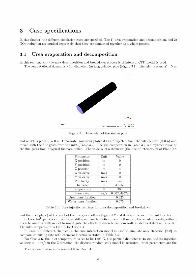
In this section, only the urea decomposition and breakdown process is of interest. CFD model is used.The computational domain is a 1m diameter, 5m long cylinder pipe (Figure 3.1). The inlet is plane Z = 5 m
Figure 3.1: Geometry of the simple pipe
and outlet is plain Z = 0 m. Urea-water mixtures (Table 3.1) are injected from the inlet center, (0, 0, 5) andmixed with the flue gases from the inlet (Table 3.2). The gas composition in Table 3.2 is a representative ofthe flue gases from a typical biomass boiler. The velocity of a diameter (the line of intersection of Plane XZ
Parameter Unit ValueX position m 0Y position m 0Z position m 4X velocity m/s 0Y velocity m/s 0Z velocity m/s -25Diameter m 4.5E-5
Temperature K 300Flow rate kg/s 0.002348578
Urea mass fraction 0.325Water mass fraction 0.675
Table 3.1: Urea injection settings for urea decomposition and breakdown
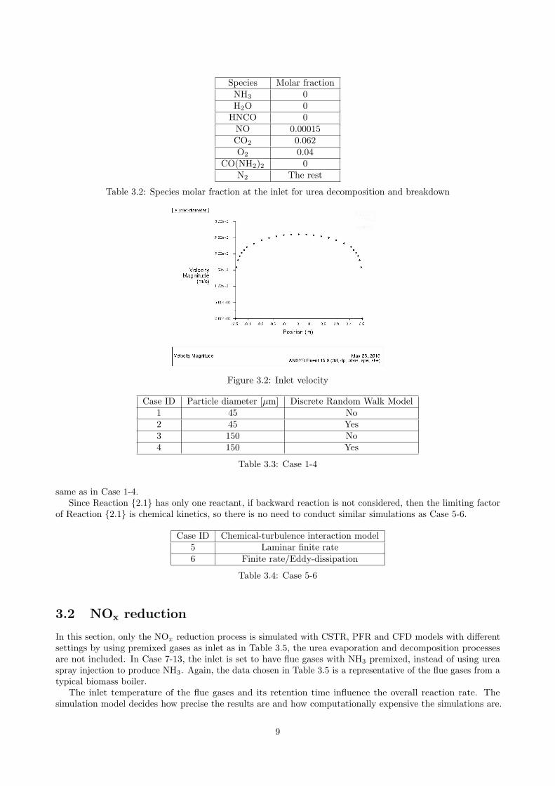
and the inlet plane) at the inlet of the flue gases follows Figure 3.2 and it is symmetric of the inlet center.In Case 1-41, particles are set to two different diameters (45 mm and 150 mm) in the simulation with/without
discrete random walk model to investigate the effects of discrete random walk model as stated in Table 3.3.The inlet temperature is 1173 K for Case 1-4.
In Case 5-6, different chemical-turbulence interaction model is used to simulate only Reaction {2.2} tocompare its mixing rate with chemical kinetics as stated in Table 3.4.
For Case 5-6, the inlet temperature is set to be 1223 K, the particle diameter is 45 µm and its injectionvelocity is −5 m/s in the Z-direction, the discrete random walk model is activated, other parameters are the
1The O2 molar fraction at the inlet is 0.12 for Case 1-4.
8
Species Molar fractionNH3 0H2O 0
HNCO 0NO 0.00015CO2 0.062O2 0.04
CO(NH2)2 0N2 The rest
Table 3.2: Species molar fraction at the inlet for urea decomposition and breakdown
Figure 3.2: Inlet velocity
Case ID Particle diameter [µm] Discrete Random Walk Model1 45 No2 45 Yes3 150 No4 150 Yes
Table 3.3: Case 1-4
same as in Case 1-4.Since Reaction {2.1} has only one reactant, if backward reaction is not considered, then the limiting factor
of Reaction {2.1} is chemical kinetics, so there is no need to conduct similar simulations as Case 5-6.
Case ID Chemical-turbulence interaction model5 Laminar finite rate6 Finite rate/Eddy-dissipation
Table 3.4: Case 5-6
3.2 NOx reduction
In this section, only the NOx reduction process is simulated with CSTR, PFR and CFD models with differentsettings by using premixed gases as inlet as in Table 3.5, the urea evaporation and decomposition processesare not included. In Case 7-13, the inlet is set to have flue gases with NH3 premixed, instead of using ureaspray injection to produce NH3. Again, the data chosen in Table 3.5 is a representative of the flue gases from atypical biomass boiler.
The inlet temperature of the flue gases and its retention time influence the overall reaction rate. Thesimulation model decides how precise the results are and how computationally expensive the simulations are.
9
Species Molar fractionNH3 0.00015H2O 0
HNCO 0NO 0.00015CO2 0.062O2 0.04
CO(NH2)2 0N2 The rest
Table 3.5: Species molar fraction at the inlet for NOx reduction
Based on the effects of inlet temperature and the simulation models, the cases in Table 3.6 are simulated withdifferent inlet temperature and simulation models. By analyzing the data at difference positions, the effects ofretention time can be investigated.
For Case 7-11, the discrete random walk model is activated and finite rate/eddy-dissipation is used aschemical-turbulence interaction model.
For Case 12-132, the inlet conditions are the same as in Case 8.
Case ID Inlet temperature [K] Simulation model7 1173 CFD8 1223 CFD9 1273 CFD10 1323 CFD11 1373 CFD12 1223 CSTR13 1223 PFR
Table 3.6: Case 7-13
Similar to Case 5-6, Case 14-17 are set to determine the impacts of mixing and chemical kinetics of Reaction{2.3} and Reaction {2.4}.
However, in Case 14-17, Reaction {2.1} and {2.2} are included and the inlet and injection conditions areas the same as in Case 5-6. If the the premixed flue gases with NH3 as inlet, the simulation results will notdiffer whether laminar finite rate model or finite rate/eddy-dissipation model is used as chemical-turbulenceinteraction model. In each case, only one reaction of Reaction {2.3} or {2.4} is simulated in the CFD model.
In this section, the whole process, meaning urea evaporation and decomposition and NOx reduction all together,is simulated.
21223K is used based on the results that are shown in Figure 4.4: 1223K is the optimum temperature for NOx reduction on thegiven conditions.
10
3.3.1 Simple pipe
In this part, the whole process is simulated in the CFD model. The inlet temperature is set to be 1223 K,the particle diameter is 45 µm and its injection velocity is −25 m/s in the Z-direction, the discrete randomwalk model is activated, finite rate/eddy-dissipation is used as chemical-turbulence interaction model, otherparameters are the same as in Case 1-4.
Case ID 18Temperature [K] 1223
Chemical-turbulence interaction model Finite rate/Eddy-dissipation
Table 3.8: Case 18
3.3.2 Rorvik plant
In this section, a new geometry based on a real power plant Rorvik is used in the simulation as seen in Figure3.3.
Figure 3.3: Geometry of the Rovik power plant urea SNCR system
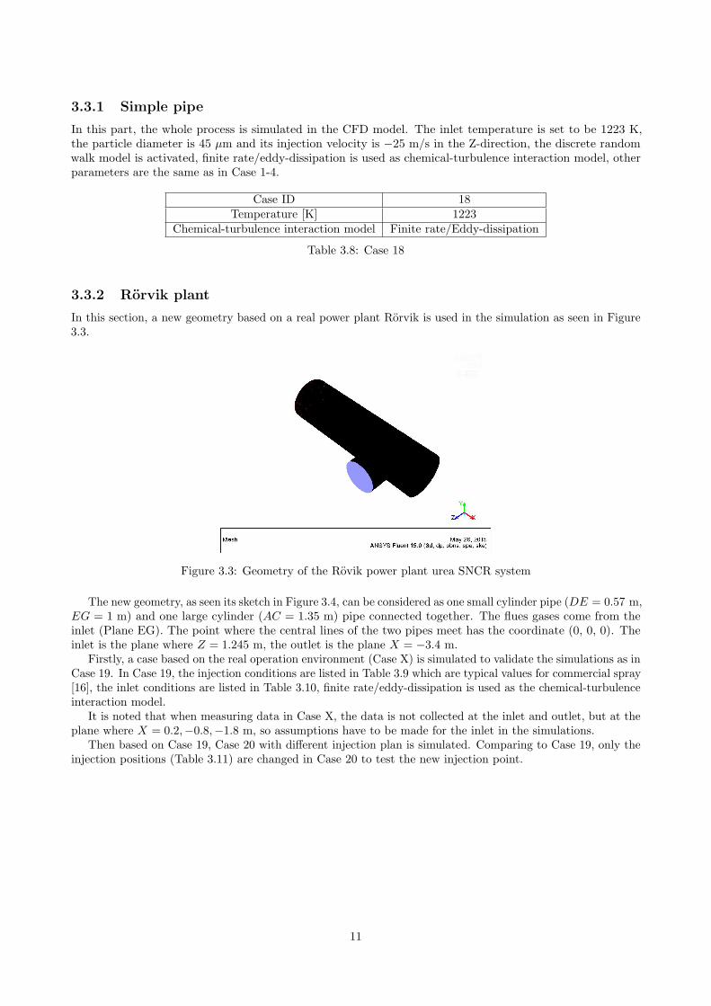
The new geometry, as seen its sketch in Figure 3.4, can be considered as one small cylinder pipe (DE = 0.57 m,EG = 1 m) and one large cylinder (AC = 1.35 m) pipe connected together. The flues gases come from theinlet (Plane EG). The point where the central lines of the two pipes meet has the coordinate (0, 0, 0). Theinlet is the plane where Z = 1.245 m, the outlet is the plane X = −3.4 m.
Firstly, a case based on the real operation environment (Case X) is simulated to validate the simulations as inCase 19. In Case 19, the injection conditions are listed in Table 3.9 which are typical values for commercial spray[16], the inlet conditions are listed in Table 3.10, finite rate/eddy-dissipation is used as the chemical-turbulenceinteraction model.
It is noted that when measuring data in Case X, the data is not collected at the inlet and outlet, but at theplane where X = 0.2,−0.8,−1.8 m, so assumptions have to be made for the inlet in the simulations.
Then based on Case 19, Case 20 with different injection plan is simulated. Comparing to Case 19, only theinjection positions (Table 3.11) are changed in Case 20 to test the new injection point.
11
Figure 3.4: Sketch of Figure 3.3 in Y direction
Parameter Unit ValueX position m 0.3Y position m 0Z position m 1.244X velocity m/s -17.75Y velocity m/s 0Z velocity m/s 0Diameter m 0.0001
Temperature K 300Flow rate kg/s 0.001240555
Urea mass fraction 0.3506Water mass fraction 0.6494
Case ID Injection positions [m]19 (0.3, 0, 1.244)20 (-0.5, 0, 0.475)
Table 3.11: Injection positions for Case 19-20
12
4 Results and discussions
Results based on the previous case specifications are presented and discussed in this chapter.
4.1 Effects of discrete random walk model on urea spray injectionsimulation
In the section, a brief summary of the results (that are based on Case 1-4) in Appended Paper A is presented.
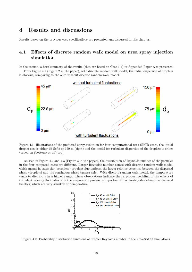
From Figure 4.1 (Figure 2 in the paper), with discrete random walk model, the radial dispersion of dropletsis obvious, comparing to the ones without discrete random walk model.
Figure 4.1: Illustrations of the predicted spray evolution for four computational urea-SNCR cases, the initialdroplet size is either 45 (left) or 150 m (right) and the model for turbulent dispersion of the droplets is eitherturned on (bottom) or off (top)
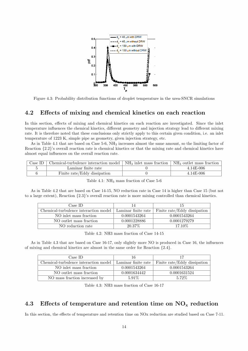
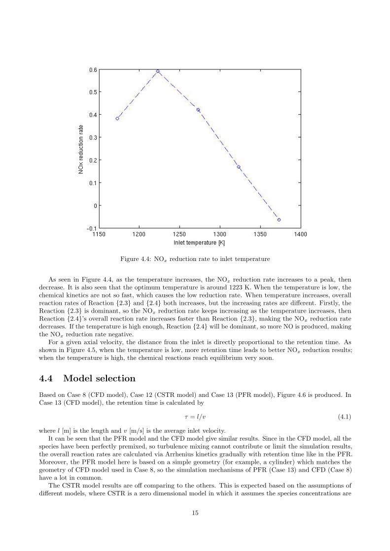
As seen in Figure 4.2 and 4.3 (Figure 3 in the paper), the distribution of Reynolds number of the particlesin the four compared cases are different. Larger Reynolds number comes with discrete random walk model,which means in cases that considers turbulent fluctuations, the larger relative velocities between the dispersedphase (droplets) and the continuous phase (gases) exist. With discrete random walk model, the temperaturetends to distribute in a higher range. These observations indicate that a proper modeling of the effects ofturbulent velocity fluctuations on the evaporation process is important for accurately describing the chemicalkinetics, which are very sensitive to temperature.
Figure 4.2: Probability distribution functions of droplet Reynolds number in the urea-SNCR simulations
13
Figure 4.3: Probability distribution functions of droplet temperature in the urea-SNCR simulations
4.2 Effects of mixing and chemical kinetics on each reaction
In this section, effects of mixing and chemical kinetics on each reaction are investigated. Since the inlettemperature influences the chemical kinetics, different geometry and injection strategy lead to different mixingrate. It is therefore noted that these conclusions only strictly apply to this certain given condition, i.e. an inlettemperature of 1223 K, simple pipe as geometry, given injection strategy, etc.
As in Table 4.1 that are based on Case 5-6, NH3 increases almost the same amount, so the limiting factor ofReaction {2.2}’s overall reaction rate is chemical kinetics or that the mixing rate and chemical kinetics havealmost equal influences on the overall reaction rate.
Case ID Chemical-turbulence interaction model NH3 inlet mass fraction NH3 outlet mass fraction5 Laminar finite rate 0 4.14E-0066 Finite rate/Eddy dissipation 0 4.14E-006
Table 4.1: NH3 mass fraction of Case 5-6
As in Table 4.2 that are based on Case 14-15, NO reduction rate in Case 14 is higher than Case 15 (but notto a large extent), Reaction {2.3}’s overall reaction rate is more mixing controlled than chemical kinetics.
Case ID 14 15Chemical-turbulence interaction model Laminar finite rate Finite rate/Eddy dissipation
NO inlet mass fraction 0.0001543264 0.0001543264NO outlet mass fraction 0.0001228886 0.0001279279
NO reduction rate 20.37% 17.10%
Table 4.2: NH3 mass fraction of Case 14-15
As in Table 4.3 that are based on Case 16-17, only slightly more NO is produced in Case 16, the influencesof mixing and chemical kinetics are almost in the same order for Reaction {2.4}.
Case ID 16 17Chemical-turbulence interaction model Laminar finite rate Finite rate/Eddy dissipation
NO inlet mass fraction 0.0001543264 0.0001543264NO outlet mass fraction 0.0001634442 0.0001631524
NO mass fraction increased by 5.91% 5.72%
Table 4.3: NH3 mass fraction of Case 16-17
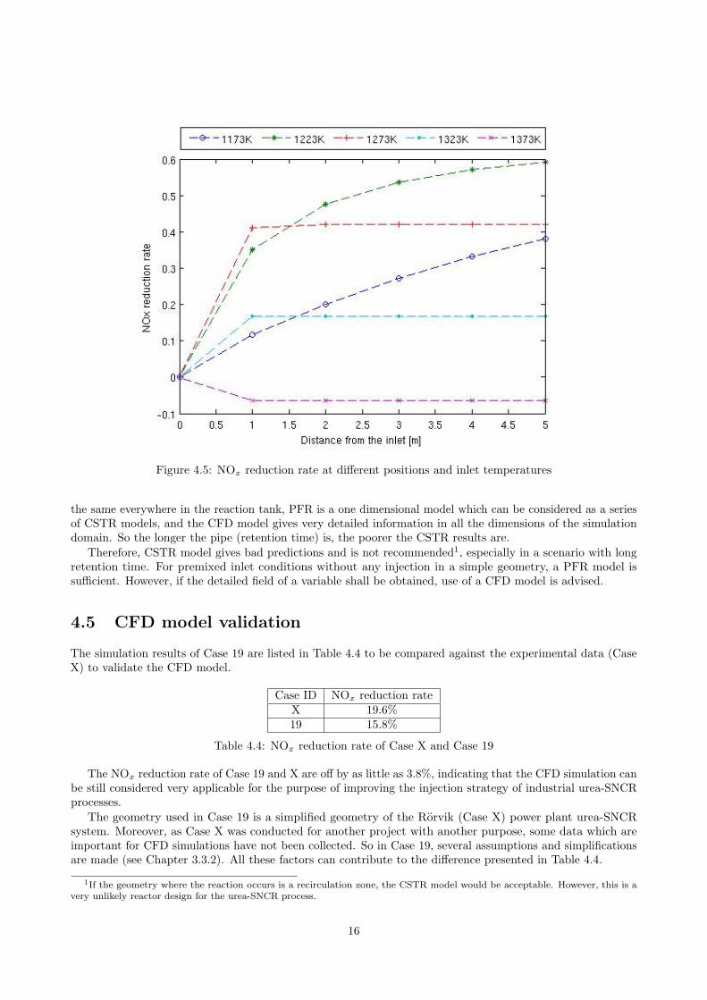
4.3 Effects of temperature and retention time on NOx reduction
In this section, the effects of temperature and retention time on NOx reduction are studied based on Case 7-11.
14
Figure 4.4: NOx reduction rate to inlet temperature
As seen in Figure 4.4, as the temperature increases, the NOx reduction rate increases to a peak, thendecrease. It is also seen that the optimum temperature is around 1223 K. When the temperature is low, thechemical kinetics are not so fast, which causes the low reduction rate. When temperature increases, overallreaction rates of Reaction {2.3} and {2.4} both increases, but the increasing rates are different. Firstly, theReaction {2.3} is dominant, so the NOx reduction rate keeps increasing as the temperature increases, thenReaction {2.4}’s overall reaction rate increases faster than Reaction {2.3}, making the NOx reduction ratedecreases. If the temperature is high enough, Reaction {2.4} will be dominant, so more NO is produced, makingthe NOx reduction rate negative.
For a given axial velocity, the distance from the inlet is directly proportional to the retention time. Asshown in Figure 4.5, when the temperature is low, more retention time leads to better NOx reduction results;when the temperature is high, the chemical reactions reach equilibrium very soon.
4.4 Model selection
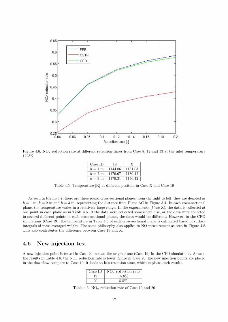
Based on Case 8 (CFD model), Case 12 (CSTR model) and Case 13 (PFR model), Figure 4.6 is produced. InCase 13 (CFD model), the retention time is calculated by
τ = l/v (4.1)
where l [m] is the length and v [m/s] is the average inlet velocity.It can be seen that the PFR model and the CFD model give similar results. Since in the CFD model, all the
species have been perfectly premixed, so turbulence mixing cannot contribute or limit the simulation results,the overall reaction rates are calculated via Arrhenius kinetics gradually with retention time like in the PFR.Moreover, the PFR model here is based on a simple geometry (for example, a cylinder) which matches thegeometry of CFD model used in Case 8, so the simulation mechanisms of PFR (Case 13) and CFD (Case 8)have a lot in common.
The CSTR model results are off comparing to the others. This is expected based on the assumptions ofdifferent models, where CSTR is a zero dimensional model in which it assumes the species concentrations are
15
Figure 4.5: NOx reduction rate at different positions and inlet temperatures
the same everywhere in the reaction tank, PFR is a one dimensional model which can be considered as a seriesof CSTR models, and the CFD model gives very detailed information in all the dimensions of the simulationdomain. So the longer the pipe (retention time) is, the poorer the CSTR results are.
Therefore, CSTR model gives bad predictions and is not recommended1, especially in a scenario with longretention time. For premixed inlet conditions without any injection in a simple geometry, a PFR model issufficient. However, if the detailed field of a variable shall be obtained, use of a CFD model is advised.
4.5 CFD model validation
The simulation results of Case 19 are listed in Table 4.4 to be compared against the experimental data (CaseX) to validate the CFD model.
Case ID NOx reduction rateX 19.6%19 15.8%
Table 4.4: NOx reduction rate of Case X and Case 19
The NOx reduction rate of Case 19 and X are off by as little as 3.8%, indicating that the CFD simulation canbe still considered very applicable for the purpose of improving the injection strategy of industrial urea-SNCRprocesses.
The geometry used in Case 19 is a simplified geometry of the Rorvik (Case X) power plant urea-SNCRsystem. Moreover, as Case X was conducted for another project with another purpose, some data which areimportant for CFD simulations have not been collected. So in Case 19, several assumptions and simplificationsare made (see Chapter 3.3.2). All these factors can contribute to the difference presented in Table 4.4.
1If the geometry where the reaction occurs is a recirculation zone, the CSTR model would be acceptable. However, this is avery unlikely reactor design for the urea-SNCR process.
16
Figure 4.6: NOx reduction rate at different retention times from Case 8, 12 and 13 at the inlet temperature1223K
Case ID 19 Xh = 1 m 1144.86 1131.03h = 2 m 1179.67 1180.42h = 3 m 1179.31 1146.42
Table 4.5: Temperature [K] at different position in Case X and Case 19
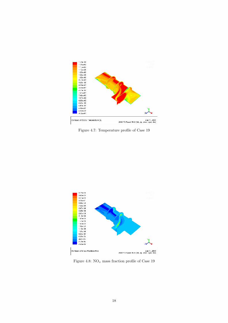
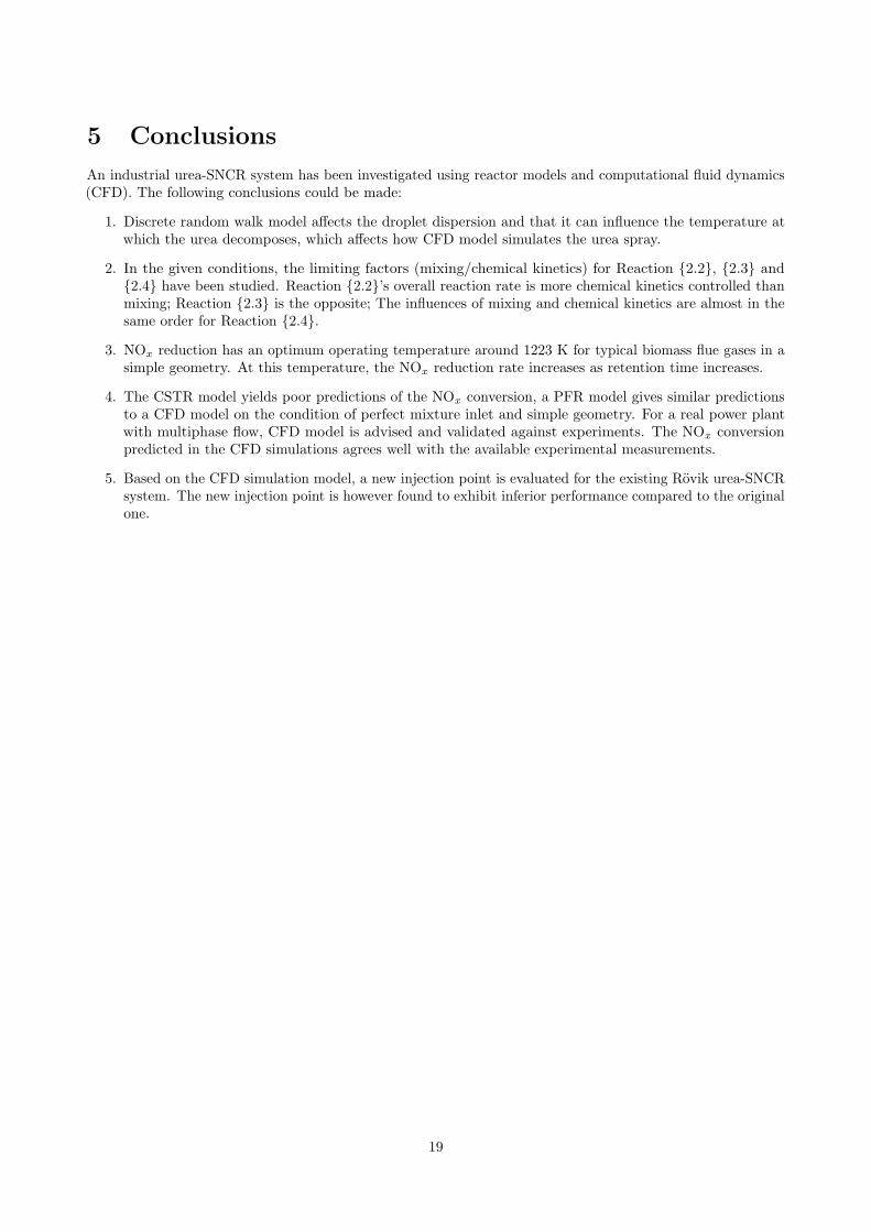
As seen in Figure 4.7, there are three round cross-sectional planes, from the right to left, they are denoted ash = 1 m, h = 2 m and h = 3 m, representing the distance from Plane AC in Figure 3.4. In each cross-sectionalplane, the temperature varies in a relatively large range. In the experiments (Case X), the data is collected atone point in each plane as in Table 4.5. If the data were collected somewhere else, or the data were collectedin several different points in each cross-sectional planes, the data would be different. However, in the CFDsimulations (Case 19), the temperature in Table 4.5 of each cross-sectional plane is calculated based of surfaceintegrals of mass-averaged weight. The same philosophy also applies to NO measurement as seen in Figure 4.8.This also contributes the difference between Case 19 and X.
4.6 New injection test
A new injection point is tested in Case 20 instead the original one (Case 19) in the CFD simulations. As seenthe results in Table 4.6, the NOx reduction rate is lower. Since in Case 20, the new injection points are placedin the downflow compare to Case 19, it leads to less retention time, which explains such results.
Case ID NOx reduction rate19 15.8%20 5.5%
Table 4.6: NOx reduction rate of Case 19 and 20
17
Figure 4.7: Temperature profile of Case 19
Figure 4.8: NOx mass fraction profile of Case 19
18
5 Conclusions
An industrial urea-SNCR system has been investigated using reactor models and computational fluid dynamics(CFD). The following conclusions could be made:
1. Discrete random walk model affects the droplet dispersion and that it can influence the temperature atwhich the urea decomposes, which affects how CFD model simulates the urea spray.
2. In the given conditions, the limiting factors (mixing/chemical kinetics) for Reaction {2.2}, {2.3} and{2.4} have been studied. Reaction {2.2}’s overall reaction rate is more chemical kinetics controlled thanmixing; Reaction {2.3} is the opposite; The influences of mixing and chemical kinetics are almost in thesame order for Reaction {2.4}.
3. NOx reduction has an optimum operating temperature around 1223 K for typical biomass flue gases in asimple geometry. At this temperature, the NOx reduction rate increases as retention time increases.
4. The CSTR model yields poor predictions of the NOx conversion, a PFR model gives similar predictionsto a CFD model on the condition of perfect mixture inlet and simple geometry. For a real power plantwith multiphase flow, CFD model is advised and validated against experiments. The NOx conversionpredicted in the CFD simulations agrees well with the available experimental measurements.
5. Based on the CFD simulation model, a new injection point is evaluated for the existing Rovik urea-SNCRsystem. The new injection point is however found to exhibit inferior performance compared to the originalone.
19
6 Future work
In this chapter, several improvements for the continuation of this work are proposed.Better chemical reaction mechanism can be used. For example, the two-step NOx reduction process can be
simulated based on the work of Farcy et al. [17].Different CFD models can be tested (such as, using DES model instead k − ε, change to different discrete
random walk model) to see if it is worthwhile to use more complicated models to simulate the process.It is also interesting to see investigate the turbulence mixing and chemical mechanism in detail at different
temperatures. Similar model to discrete random walk model can be also deployed to account for the turbulenttemperature and species concentrations fluctuations on the reaction rates.
When conducting experiment in the real power plant, data that are crucial to the simulation works shouldbe collected, so the simulation models can be more comprehensively validated.
20
References
[1] A. Fritz and V. Pitchon. The current state of research on automotive lean NOx catalysis. 1997. doi:10.1016/S0926-3373(96)00102-6.
[2] S. S. Sazhin. Advanced models of fuel droplet heating and evaporation. Progress in Energy and CombustionScience 32.2 (Jan. 2006), 162–214. doi: 10.1016/j.pecs.2005.11.001.
[3] R. Miller, K. Harstad, and J. Bellan. Evaluation of equilibrium and non-equilibrium evaporation modelsfor many-droplet gas-liquid flow simulations. International Journal of Multiphase Flow 24.6 (Sept. 1998),1025–1055. doi: 10.1016/S0301-9322(98)00028-7.
[4] A. Lundstrom et al. Modelling of urea gas phase thermolysis and theoretical details on urea evaporation.2011.
[5] M. Østberg and K. Dam-Johansen. Empirical modeling of the selective non-catalytic reduction of no:comparison with large-scale experiments and detailed kinetic modeling. Chemical Engineering Science49.12 (June 1994), 1897–1904. doi: 10.1016/0009-2509(94)80074-X.
[6] R. Rota et al. Experimental and modeling analysis of the NOxOUT process. Chemical EngineeringScience 57.1 (Jan. 2002), 27–38. doi: 10.1016/S0009-2509(01)00367-0.
[7] G. W. Roberts. Chemical reactions and chemical reactors. John Wiley & Sons Hoboken, 2009.[8] B. Andersson et al. Computational Fluid Dynamics for Engineers. 2011.[9] H. K. Versteeg and W. Malalasekera. An Introduction to Computational Fluid Dynamics: The Finite
Volume Method. 2007.[10] B. Launder and D. Spalding. The numerical computation of turbulent flows. Computer Methods in Applied
Mechanics and Engineering 3.2 (Mar. 1974), 269–289. doi: 10.1016/0045-7825(74)90029-2.[11] S. Arrhenius. Uber die Dissociationswarme und den Einfluss der Temperatur auf den Dissociationsgrad
der Elektrolyte (1889).[12] S. Arrhenius. Uber die Reaktionsgeschwindigkeit bei der Inversion von Rohrzucker durch Sauren. Zeitschrift
fur physikalische Chemie (1889).[13] B. Magnussen and B. Hjertager. On mathematical modeling of turbulent combustion with special emphasis
on soot formation and combustion. 1977.[14] A. D. Gosman and E. Ioannides. ASPECTS OF COMPUTER SIMULATION OF LIQUID-FUELED
COMBUSTORS. 1983.[15] L. T. Choi et al. Flow and particle deposition patterns in a realistic human double bifurcation airway
model. Inhalation toxicology 19.2 (2007), 117–131.[16] H. Strom, A. Lundstrom, and B. Andersson. Choice of urea-spray models in CFD simulations of urea-SCR
systems. Chemical Engineering Journal 150.1 (2009), 69–82.[17] B. Farcy et al. Two approaches of chemistry downsizing for simulating selective non catalytic reduction
droplet size is either 45 (left) or 150 m (right) and the model for turbulent dispersion of thedroplets is either turned on (bottom) or off (top) . . . . . . . . . . . . . . . . . . . . . . . . . . 13
4.2 Probability distribution functions of droplet Reynolds number in the urea-SNCR simulations . 134.3 Probability distribution functions of droplet temperature in the urea-SNCR simulations . . . . 144.4 NOx reduction rate to inlet temperature . . . . . . . . . . . . . . . . . . . . . . . . . . . . . . . 154.5 NOx reduction rate at different positions and inlet temperatures . . . . . . . . . . . . . . . . . 164.6 NOx reduction rate at different retention times from Case 8, 12 and 13 at the inlet temperature
Appended Paper AEffect of Turbulent Velocity Fluctuations on the Convective Heat Transfer to Droplets
Subjected to Evaporation and Thermolysis (Accepted by AIP Conference Proceedings)
The Effect of Turbulent Velocity Fluctuations on the Convective Heat Transfer to Droplets Subjected to
Evaporation and Thermolysis
Ning Guo, Oskar Finnerman and Henrik Ström
Division of Fluid Dynamics, Department of Applied Mechanics Chalmers University of Technology, SE-412 96 Gothenburg, Sweden
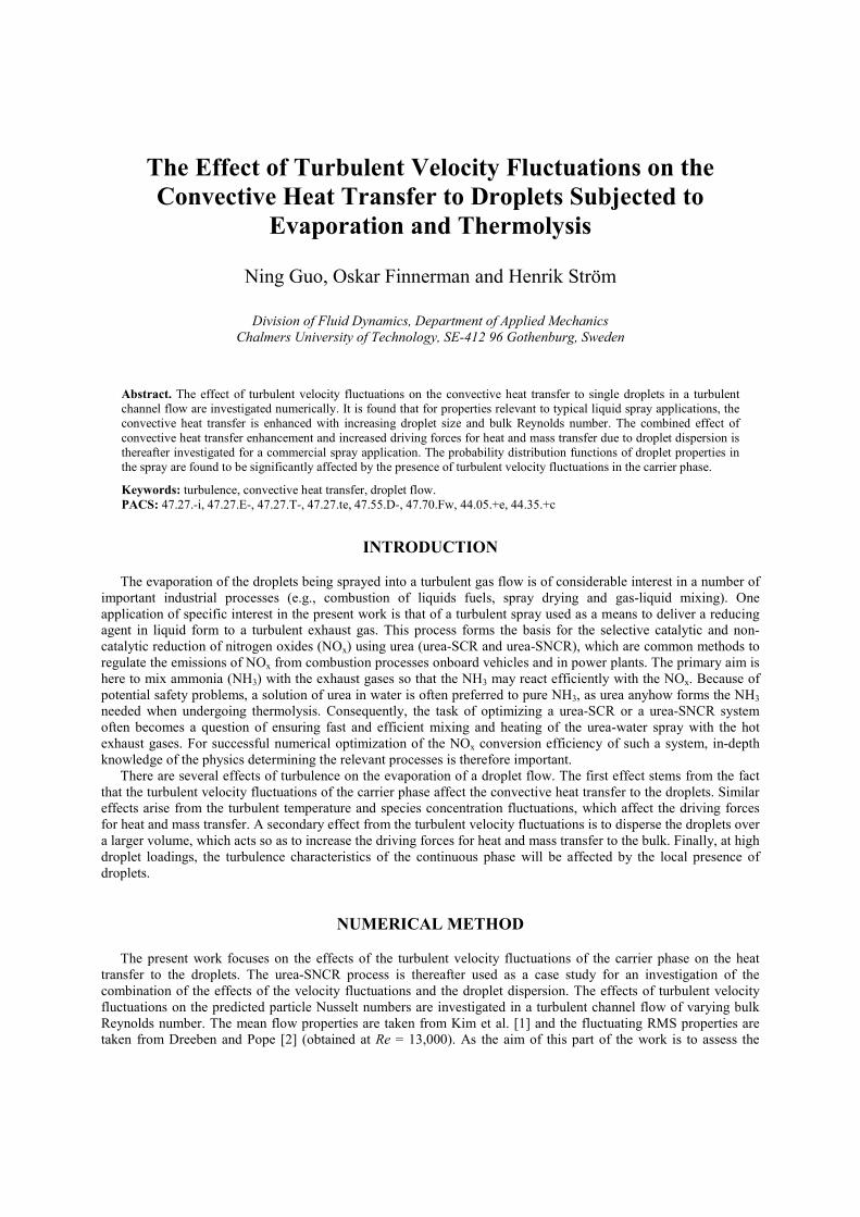
Abstract. The effect of turbulent velocity fluctuations on the convective heat transfer to single droplets in a turbulent channel flow are investigated numerically. It is found that for properties relevant to typical liquid spray applications, the convective heat transfer is enhanced with increasing droplet size and bulk Reynolds number. The combined effect of convective heat transfer enhancement and increased driving forces for heat and mass transfer due to droplet dispersion is thereafter investigated for a commercial spray application. The probability distribution functions of droplet properties in the spray are found to be significantly affected by the presence of turbulent velocity fluctuations in the carrier phase.
The evaporation of the droplets being sprayed into a turbulent gas flow is of considerable interest in a number of important industrial processes (e.g., combustion of liquids fuels, spray drying and gas-liquid mixing). One application of specific interest in the present work is that of a turbulent spray used as a means to deliver a reducing agent in liquid form to a turbulent exhaust gas. This process forms the basis for the selective catalytic and non-catalytic reduction of nitrogen oxides (NOx) using urea (urea-SCR and urea-SNCR), which are common methods to regulate the emissions of NOx from combustion processes onboard vehicles and in power plants. The primary aim is here to mix ammonia (NH3) with the exhaust gases so that the NH3 may react efficiently with the NOx. Because of potential safety problems, a solution of urea in water is often preferred to pure NH3, as urea anyhow forms the NH3 needed when undergoing thermolysis. Consequently, the task of optimizing a urea-SCR or a urea-SNCR system often becomes a question of ensuring fast and efficient mixing and heating of the urea-water spray with the hot exhaust gases. For successful numerical optimization of the NOx conversion efficiency of such a system, in-depth knowledge of the physics determining the relevant processes is therefore important.
There are several effects of turbulence on the evaporation of a droplet flow. The first effect stems from the fact that the turbulent velocity fluctuations of the carrier phase affect the convective heat transfer to the droplets. Similar effects arise from the turbulent temperature and species concentration fluctuations, which affect the driving forces for heat and mass transfer. A secondary effect from the turbulent velocity fluctuations is to disperse the droplets over a larger volume, which acts so as to increase the driving forces for heat and mass transfer to the bulk. Finally, at high droplet loadings, the turbulence characteristics of the continuous phase will be affected by the local presence of droplets.
NUMERICAL METHOD
The present work focuses on the effects of the turbulent velocity fluctuations of the carrier phase on the heat transfer to the droplets. The urea-SNCR process is thereafter used as a case study for an investigation of the combination of the effects of the velocity fluctuations and the droplet dispersion. The effects of turbulent velocity fluctuations on the predicted particle Nusselt numbers are investigated in a turbulent channel flow of varying bulk Reynolds number. The mean flow properties are taken from Kim et al. [1] and the fluctuating RMS properties are taken from Dreeben and Pope [2] (obtained at Re = 13,000). As the aim of this part of the work is to assess the
magnitude of the influences of the turbulent velocity fluctuations, the Reynolds-number dependence of the fluctuating quantities is disregarded. This assumption is expected to lead to an underestimation of the streamwise fluctuations and a (smaller) overestimation of the wall-normal fluctuations, as shown by Wei and Willmarth [3]. The overall conclusion is thus that the use of RMS property correlations obtained at a fixed bulk Reynolds number will tend to produce conservative estimates.
For each bulk Reynolds number, the complete Nusselt number history is acquired for an ensemble of 10,000 particles over a time period equal to 100 times the particle response time. The particles are introduced at random locations over the duct cross-section at the local mean velocity of the gas and are assumed to rebound in inelastic collisions upon interaction with the wall. The particle position is updated from knowing its velocity, and the particle velocity is obtained from:
( )( )pppp
p uuuReddt
du−′++= 687.0
2 15.0118ρ
µ (1)
Here, up is the particle velocity, µ is the dynamic viscosity of the gas phase, ρp is the particle density, dp is the
particle diameter, Rep is the particle Reynolds number, u is the gas phase mean velocity and u′ is the current gas phase velocity fluctuation (both taken at the current location of the particle). The formulation used in equation (1) reflects the fact that the drag correlation of Schiller and Naumann is employed [4]. The time step used in the integration of these equations is two orders of magnitude smaller than the particle response time. The gas phase velocity fluctuation is updated according to an eddy-interaction model [5] as described by Dehbi [6]. The anisotropy of the velocity fluctuations in the near-wall region is correctly accounted for by the present method, and the random insertion of particles into the duct enables the acquisition of averaged data, representative for the complete system.
The Nusselt number correlation used to assess the turbulent effects on heat transfer is taken from Frössling [7]:
315.0 Pr552.02 pReNu += (2) In a case where turbulent velocity fluctuations are not accounted for, the inserted particles would simply follow
the gas flow at zero relative velocity, resulting in a constant Nusselt number equal to 2. The Nusselt number history obtained for each particle is therefore compared to this value to determine the time-averaged increase in the Nusselt number.
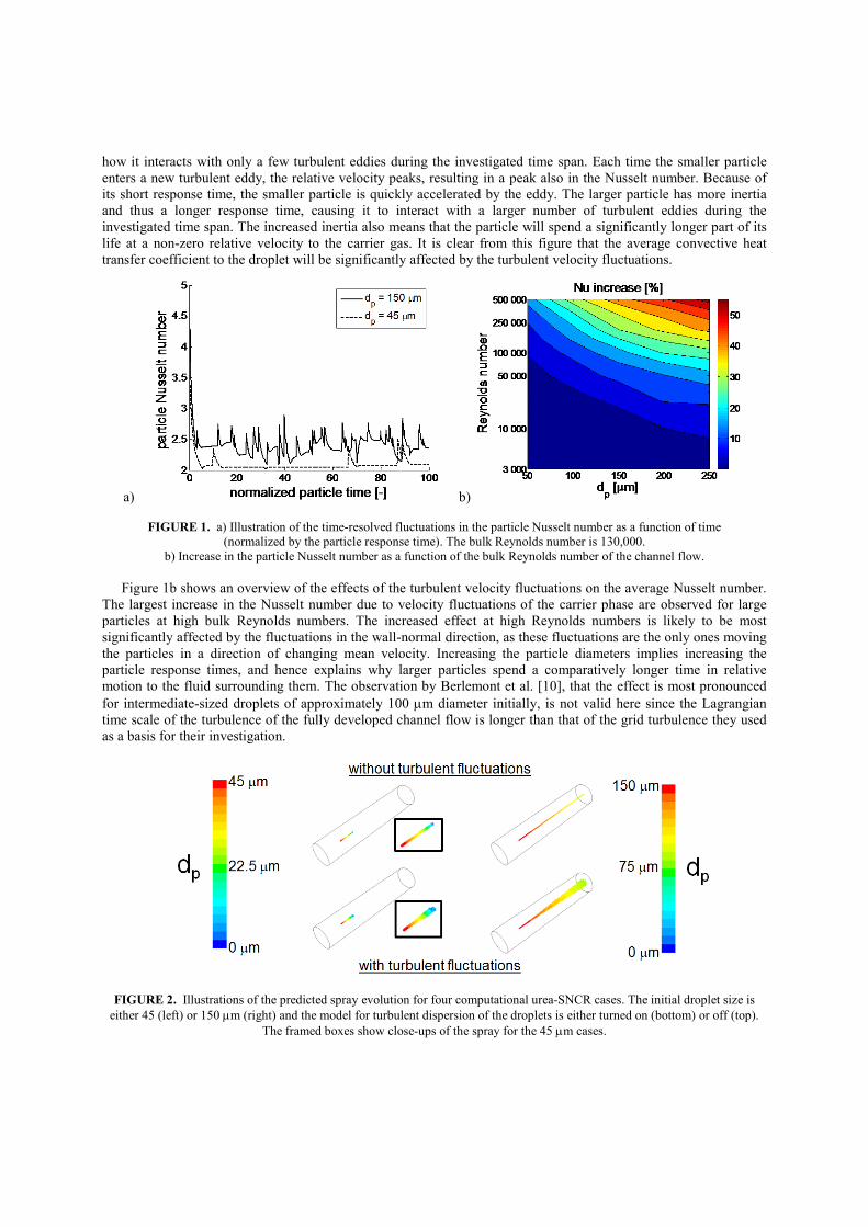
The effects of turbulent velocity fluctuations, modeled via an eddy-interaction model, are also investigated in a commercial urea-SNCR process. The injection of the urea-water solution will result in two processes – evaporation of water and thermolysis of urea [8] – that are both heat-transfer limited and that can both be modeled as evaporation processes [9]. The non-isothermal, chemically reactive turbulent gas flow is modeled using the Standard k-ε turbulence model. The effects of velocity fluctuations on the droplet trajectories and heat transfer coefficients are accounted for via the Discrete Random Walk (DRW) model [6]. Two-way coupling is employed between the gas phase and the droplet phase, so that the secondary effect of the droplet dispersion (via the temperature and concentration fields) is accounted for as well. Turbulent fluctuations of the temperature and the species concentrations and turbulence modulation from the presence of droplets are neglected, however. It is to be expected that the effect of species concentration fluctuations is negligible, whereas the effect of temperature fluctuations, if included, would act so as to further increase the broadening of the particle diameter probability distribution function [10]. The injected droplets are assumed to follow a uniform diameter distribution of either 45 or 150 µm. The initial urea content is 32.5% by weight, the rest is water. The droplets are injected at 300K into exhaust of 1173K. The exhaust gases flow through a circular duct of 1 m diameter and 5 m length. The injector is located 1 m downstream the gas inlet and points in the co-current direction. The bulk Reynolds number is approximately 400,000.
RESULTS AND DISCUSSION
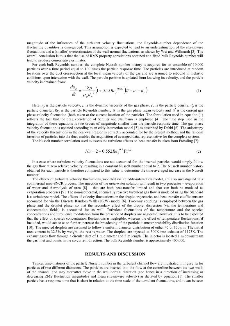
Typical time-histories of the particle Nusselt number in the turbulent channel flow are illustrated in Figure 1a for particles of two different diameters. The particles are inserted into the flow at the centerline between the two walls of the channel, and may thereafter move in the wall-normal direction (and hence in a direction of increasing or decreasing RMS fluctuation magnitudes and mean streamwise velocity) as dictated by equation (1). The smaller particle has a response time that is short in relation to the time scale of the turbulent fluctuations, and it can be seen
how it interacts with only a few turbulent eddies during the investigated time span. Each time the smaller particle enters a new turbulent eddy, the relative velocity peaks, resulting in a peak also in the Nusselt number. Because of its short response time, the smaller particle is quickly accelerated by the eddy. The larger particle has more inertia and thus a longer response time, causing it to interact with a larger number of turbulent eddies during the investigated time span. The increased inertia also means that the particle will spend a significantly longer part of its life at a non-zero relative velocity to the carrier gas. It is clear from this figure that the average convective heat transfer coefficient to the droplet will be significantly affected by the turbulent velocity fluctuations.
a) b)
FIGURE 1. a) Illustration of the time-resolved fluctuations in the particle Nusselt number as a function of time (normalized by the particle response time). The bulk Reynolds number is 130,000.
b) Increase in the particle Nusselt number as a function of the bulk Reynolds number of the channel flow. Figure 1b shows an overview of the effects of the turbulent velocity fluctuations on the average Nusselt number.
The largest increase in the Nusselt number due to velocity fluctuations of the carrier phase are observed for large particles at high bulk Reynolds numbers. The increased effect at high Reynolds numbers is likely to be most significantly affected by the fluctuations in the wall-normal direction, as these fluctuations are the only ones moving the particles in a direction of changing mean velocity. Increasing the particle diameters implies increasing the particle response times, and hence explains why larger particles spend a comparatively longer time in relative motion to the fluid surrounding them. The observation by Berlemont et al. [10], that the effect is most pronounced for intermediate-sized droplets of approximately 100 µm diameter initially, is not valid here since the Lagrangian time scale of the turbulence of the fully developed channel flow is longer than that of the grid turbulence they used as a basis for their investigation.
FIGURE 2. Illustrations of the predicted spray evolution for four computational urea-SNCR cases. The initial droplet size is either 45 (left) or 150 µm (right) and the model for turbulent dispersion of the droplets is either turned on (bottom) or off (top).
The framed boxes show close-ups of the spray for the 45 µm cases.
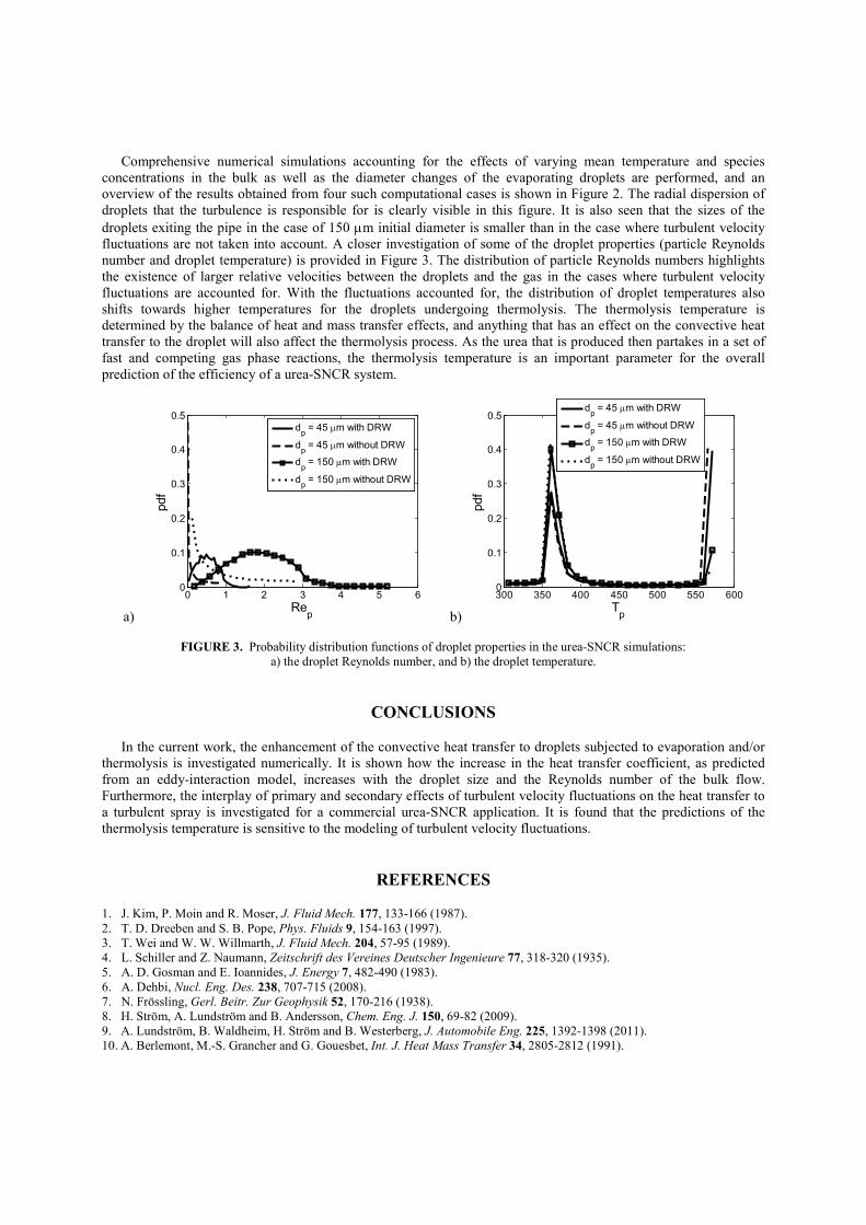
Comprehensive numerical simulations accounting for the effects of varying mean temperature and species concentrations in the bulk as well as the diameter changes of the evaporating droplets are performed, and an overview of the results obtained from four such computational cases is shown in Figure 2. The radial dispersion of droplets that the turbulence is responsible for is clearly visible in this figure. It is also seen that the sizes of the droplets exiting the pipe in the case of 150 µm initial diameter is smaller than in the case where turbulent velocity fluctuations are not taken into account. A closer investigation of some of the droplet properties (particle Reynolds number and droplet temperature) is provided in Figure 3. The distribution of particle Reynolds numbers highlights the existence of larger relative velocities between the droplets and the gas in the cases where turbulent velocity fluctuations are accounted for. With the fluctuations accounted for, the distribution of droplet temperatures also shifts towards higher temperatures for the droplets undergoing thermolysis. The thermolysis temperature is determined by the balance of heat and mass transfer effects, and anything that has an effect on the convective heat transfer to the droplet will also affect the thermolysis process. As the urea that is produced then partakes in a set of fast and competing gas phase reactions, the thermolysis temperature is an important parameter for the overall prediction of the efficiency of a urea-SNCR system.
a) b)
FIGURE 3. Probability distribution functions of droplet properties in the urea-SNCR simulations: a) the droplet Reynolds number, and b) the droplet temperature.
CONCLUSIONS
In the current work, the enhancement of the convective heat transfer to droplets subjected to evaporation and/or thermolysis is investigated numerically. It is shown how the increase in the heat transfer coefficient, as predicted from an eddy-interaction model, increases with the droplet size and the Reynolds number of the bulk flow. Furthermore, the interplay of primary and secondary effects of turbulent velocity fluctuations on the heat transfer to a turbulent spray is investigated for a commercial urea-SNCR application. It is found that the predictions of the thermolysis temperature is sensitive to the modeling of turbulent velocity fluctuations.
REFERENCES
1. J. Kim, P. Moin and R. Moser, J. Fluid Mech. 177, 133-166 (1987). 2. T. D. Dreeben and S. B. Pope, Phys. Fluids 9, 154-163 (1997). 3. T. Wei and W. W. Willmarth, J. Fluid Mech. 204, 57-95 (1989). 4. L. Schiller and Z. Naumann, Zeitschrift des Vereines Deutscher Ingenieure 77, 318-320 (1935). 5. A. D. Gosman and E. Ioannides, J. Energy 7, 482-490 (1983). 6. A. Dehbi, Nucl. Eng. Des. 238, 707-715 (2008). 7. N. Frössling, Gerl. Beitr. Zur Geophysik 52, 170-216 (1938). 8. H. Ström, A. Lundström and B. Andersson, Chem. Eng. J. 150, 69-82 (2009). 9. A. Lundström, B. Waldheim, H. Ström and B. Westerberg, J. Automobile Eng. 225, 1392-1398 (2011). 10. A. Berlemont, M.-S. Grancher and G. Gouesbet, Int. J. Heat Mass Transfer 34, 2805-2812 (1991).