Georgetown University Law Center Georgetown University Law Center Scholarship @ GEORGETOWN LAW Scholarship @ GEORGETOWN LAW 2015 cGUPPI: Scoring Incentives to Engage in Parallel Accommodating cGUPPI: Scoring Incentives to Engage in Parallel Accommodating Conduct Conduct Serge Moresi Charles River Associates (CRA), [email protected]David Reitman Charles River Associates (CRA), [email protected]Steven C. Salop Georgetown University Law Center, [email protected]Yianis Sarafidis Charles River Associates (CRA), ysarafi[email protected]This paper can be downloaded free of charge from: https://scholarship.law.georgetown.edu/facpub/1501 http://ssrn.com/abstract=2640962 This open-access article is brought to you by the Georgetown Law Library. Posted with permission of the author. Follow this and additional works at: https://scholarship.law.georgetown.edu/facpub Part of the Antitrust and Trade Regulation Commons , Business Organizations Law Commons , and the Public Economics Commons
Transcript
Georgetown University Law Center Georgetown University Law Center
Scholarship @ GEORGETOWN LAW Scholarship @ GEORGETOWN LAW
2015
cGUPPI: Scoring Incentives to Engage in Parallel Accommodating cGUPPI: Scoring Incentives to Engage in Parallel Accommodating
This open-access article is brought to you by the Georgetown Law Library. Posted with permission of the author. Follow this and additional works at: https://scholarship.law.georgetown.edu/facpub
Part of the Antitrust and Trade Regulation Commons, Business Organizations Law Commons, and the Public Economics Commons
We propose an index for scoring coordination incentives, which we call the “coordination GUPPI” or cGUPPI. While the cGUPPI can be applied to a wide range of coordinated effects concerns, it is particularly relevant for gauging concerns of parallel accommodating conduct (PAC), a concept that received due prominence in the 2010 U.S. Horizontal Merger Guidelines. PAC is a type of coordinated conduct whereby a firm raises price with the expectation—but without any prior agreement—that one or more other firms will follow and match the price increase. The cGUPPI is the highest uniform price increase that all the would-be coordinating firms would be willing to implement without side payments. A larger cGUPPI implies a more pronounced incentive and ability for firms to engage in coordinated price increases. The difference between the post- and pre-merger cGUPPI (i.e. the Delta cGUPPI) is a practical way to score the effect of a merger on coordinated effects concerns.
_____________________________________
* Moresi, Reitman and Sarafidis are Vice Presidents, Charles River Associates, Washington, DC. Salop is Professor of Economics and Law, Georgetown University Law Center, and Senior Consultant, Charles River Associates. The views expressed herein are those of the authors and do not reflect or represent the view of Charles River Associates or any of the organizations with which the authors are affiliated. This paper is a revision of our earlier unpublished article, Gauging Parallel Accommodating Conduct Concerns with the CPPI (2011). We thank Joe Farrell, Joe Harrington, Jerry Hausman, Carl Shapiro and John Woodbury for helpful comments.
2
I. Introduction
The traditional legal approach to merger analysis has long focused on concentration and market
shares as preliminary screens. However, concentration and market shares are not linked directly
to the merging parties’ post-merger incentives to engage in potentially anticompetitive conduct.
For example, the increase in the HHI generally does not relate directly to the change in unilateral
incentives caused by a merger. In recent years, economists have developed methodologies to
score the competitive impact of mergers with screening measures more directly related to the
incentives of the parties. Initial efforts at incorporating incentives involved defining the relevant
antitrust market. The efforts resulted in a more accurate “hypothetical monopolist test” that
scores the incentives of a hypothetical monopolist (or hypothetical cartel) to raise prices in
industries characterized by price competition with differentiated products.1 The 2010 U.S.
Horizontal Merger Guidelines took this “incentive scoring” approach a step further by adopting a
gross upward pricing pressure index (“GUPPI”) for scoring the unilateral incentives of merging
parties to raise price post-merger.2
1 See Michael Katz and Carl Shapiro, Critical Loss: Let’s Tell the Whole Story, 17 ANTITRUST 49 (2003); Daniel O’Brien and Abraham Wickelgren, A Critical Analysis of Critical Loss Analysis, 71 ANTITRUST L.J. 161 (2003). See also Øystein Daljord, Lars Sørgard and Øyvind Thomassen, The SSNIP Test and Market Definition with the Aggregate Diversion Ratio: A Reply to Katz and Shapiro, 4 J. COMP. L. & ECON. 263 (2008); Joseph Farrell and Carl Shapiro, Improving Critical Loss Analysis, ANTITRUST SOURCE (Feb. 2008); Serge X. Moresi, Steven C. Salop and John R. Woodbury, Implementing the Hypothetical Monopolist SSNIP Test With Multi-Product Firms, ANTITRUST SOURCE (Feb. 2008). See also U.S. Department of Justice and Federal Trade Commission, Horizontal Merger Guidelines (Issued August 19, 2010) (hereinafter “Merger Guidelines”) at note 4, available at http://www.justice.gov/atr/public/guidelines/hmg-2010.pdf. 2 Merger Guidelines at §6.1. The GUPPI methodology is based on the Bertrand model of price competition among firms selling differentiated products. It can be extended to markets where firms compete in quantities or capacity instead of price, bidding markets, and markets with congestion issues. See Serge Moresi, The Use of Upward Price Pressure Indices in Merger Analysis, ANTITRUST SOURCE, Feb. 2010; Robert Willig, Unilateral Competitive Effects of Mergers: Upward Pricing Pressure, Product Quality, and Other Extensions, 39 REV. INDUS. ORG.19 (2011). A variant of the GUPPI also can be applied to partial ownership acquisitions, including those that give the acquiring firm some degree of control over the acquired firm. Daniel P. O’Brien and Steven C. Salop, Competitive Effects of Partial Ownership: Financial Interest and Corporate Control, 67 ANTITRUST L.J. 559 (2000).
3
Incentive scoring methodologies are particularly useful when compared to simple structural
measures such as the HHI or other concentration indices. Incentive scoring makes economic
sense because antitrust analysis is premised on the assumption that firms are rational, profit-
maximizing entities. Thus, the economic incentives of the firms provide relevant information
about the likely outcomes of their combinations. While incentive scoring is not the only
information relevant for evaluating likely competitive effects, it clearly is useful evidence,
especially in the early phases of a merger investigation.
Potential anticompetitive effects of mergers have traditionally been classified by whether the
theory of harm involves unilateral conduct on the part of the merging firms (“unilateral effects”)
or coordinated interactions that extend beyond the merging firms (“coordinated effects”).
Incentive scoring devices for unilateral effects concerns such as the Compensating Marginal Cost
Reductions (CMCRs) and GUPPIs are directly related to the unilateral incentives of the merging
parties to raise prices, as are merger simulation models.3 The toolkit available for scoring the
likelihood of anticompetitive coordinated effects in a preliminary way is more limited. The use
of the four-firm concentration ratio is premised on an assumption that the top-4 firms can
coordinate. 4 The Herfindahl Hirshman Index (HHI) similarly can be loosely related to
coordination.5 Simulation models also can be used for screening coordinated effects or for a
more complete analysis, but they often require more extensive information.6
3 See Carl Shapiro, The 2010 Horizontal Merger Guidelines: From Hedgehog to Fox in Forty Years, 77 ANTITRUST L.J. 701 (2010) for a discussion and references on merger simulation, CMCR and GUPPI methodologies for scoring unilateral effects. See also Sonia Jaffe and Glen Weyl, The First-Order Approach to Merger Analysis, 5 AMER. ECON. J.: Microeconomics 188 (2013). 4 See Robert E. Dansby and Robert D. Willig, Industry Performance Gradient Indexes, 69 AMER. ECON. REV. 249 (1979). 5 Id. See also George Stigler, A Theory of Oligopoly, 72 J. POLIT. ECON. 44 (1964). 6 See, e.g., William E. Kovacic, Robert C. Marshall, Leslie M. Marx, and Steven P. Schulenberg, Quantitative Analysis of Coordinated Effects, 76 ANTITRUST L.J. 397 (2010). For a discussion and references on merger simulation models of coordinated effects, see Pierluigi Sabbatini, The Coordinated Effect of a Merger with Tacit and Egalitarian Collusion (working paper), Italian Competition Authority (February 2014).
4
In this paper, we develop an incentive scoring measure, the “coordination GUPPI” or “cGUPPI”
for short. The cGUPPI is not difficult to calculate and can provide a standardized measure. The
cGUPPI is based on several assumptions and is most useful as a preliminary screen.
The cGUPPI methodology is focused on the impact of a merger on the incentives and ability of
market participants to coordinate through parallel accommodating conduct (PAC).7 PAC
involves one firm raising price in the hope that other firms will accommodate the price increase
by following it.8 PAC is distinguished from other forms of coordinated conduct in that it does
not require a prior agreement about the coordinated interaction or desired equilibrium. Instead,
PAC is a type of “conscious parallelism” discussed in antitrust cases.9
PAC is described in the 2010 Horizontal Merger Guidelines as follows:
Parallel accommodating conduct includes situations in which each rival’s
response to competitive moves made by others is individually rational, and not
motivated by retaliation or deterrence, nor intended to sustain an agreed-upon
market outcome, but nevertheless emboldens price increases and weakens
competitive incentives to reduce prices or offer customers better terms.10
7 For an earlier version of this basic methodology, see Serge Moresi, David Reitman, Steve C. Salop and Yianis Sarafidis, Gauging Parallel Accommodating Conduct Concerns with the CPPI, (2011), available at http://papers.ssrn.com/sol3/papers.cfm?abstract_id=1924516. The cGUPPI was denoted as the CPPI (“Coordinated Price Pressure Index”) in that earlier version. 8 Parallel accommodating conduct has a long history in oligopoly theory, dating back more than seventy years. See, e.g., Robert L. Hall and Charles J. Hitch, Price Theory and Business Behavior, 2 OXFORD ECON. PAP. 12 (1939); Paul Sweezy, Demand Under Conditions of Oligopoly, 47 J. POLIT. ECON. 568 (1939); Eric Maskin and Jean Tirole, A Theory of Dynamic Oligopoly, II: Price Competition, Kinked Demand Curves, and Edgeworth Cycles, 56 ECONOMETRICA 571 (1988); Jonathan Eaton and Maxim Engers, Intertemporal Price Competition, 58 ECONOMETRICA 637 (1990). 9 See, e.g., Theatre Enterprises, Inc. v. Paramount Film Distributing Corp., 346 U.S. 537 (1954). 10 Merger Guidelines at §7.
5
This paper describes the cGUPPI methodology and its properties, including its relationship to the
GUPPI used to score unilateral effects.11 We also illustrate the mechanics of the cGUPPI
methodology with several examples of hypothetical mergers. These examples show that a
merger may increase, decrease or have no effect on PAC incentives depending on a number of
factors, including whether the merging firms are constraining PAC pre-merger. A merger also
may change PAC incentives in significant ways if the set of potentially coordinating firms
changes after the merger. In particular, a merger may increase PAC concerns when it eliminates
a “maverick” firm, but it also may reduce PAC concerns when it creates a new, more disruptive
maverick firm.12 Merger efficiencies also can alter the incentives to engage in coordinated
pricing through PAC. While incentive scoring is a preliminary screen, our simulation model
results suggest that the simple cGUPPI analysis, which assumes no unilateral effects and no
responses by rivals, provides a useful signal for the results of more general simulation models.
II. Basic cGUPPI Framework
As explained above, the cGUPPI analysis focuses on parallel accommodating conduct (PAC),
whereby one firm initiates a price increase in the expectation that other firms will match the price
increase, but without any prior agreement. The other firms choose whether or not to match the
price increase, and they anticipate that the price leader will revert to its previous price if they do
not march the price increase. At the PAC equilibrium, the coordinating firms lack the ability to
increase prices further, because at least one of them would not match any further price increase.13
11 The cGUPPI has a number of similarities with the conventional GUPPI that is used to score unilateral effects concerns. The cGUPPI similarly is formally derived within the context of a stylized oligopoly model, namely, the Bertrand price competition model with differentiated products. The cGUPPI also uses similar data, although the analysis requires data from all potential coordinating firms (not just the two merging firms). The “Delta cGUPPI” (i.e. the increase in the cGUPPI due to a merger) also is just an index that is not intended to capture every detail of the merger impact on the equilibrium outcome of a dynamic oligopoly model, but rather normally would be used in conjunction with other evidence. 12 See Jonathan B. Baker, Mavericks, Mergers, and Exclusion: Proving Coordinated Competitive Effects Under the Antitrust Laws, 77 N.Y.U. L. Rev. 135 (2002) 13 In terms of the conventional story about coordination solving a Prisoners’ Dilemma, we are focusing on the parties achieving a supracompetitive outcome. This also is similar to the informal approach suggested by Jonathan Baker, Id. at 166-73. The formal economic model underlying the cGUPPI is developed in Yuanzhu Lu and Julian Wright, Tacit Collusion with Price-Matching Punishments, 28 INT. J.
6
At the same time, we assume that any price changes are rapidly detected. As a result, no firm
has the incentive to reduce price, because it anticipates that the other coordinating firms would
quickly match that price reduction.14 It is the fear of that rapid price matching that allows the
parties to maintain the PAC outcome. However, the parties are unable to achieve the full
monopoly outcome. PAC does not permit side payments so that the PAC equilibrium prices
typically will be lower than the prices that an unconstrained cartel would choose. If there are
detection and response lags, the attainable PAC price increase is even lower.15
In deriving the cGUPPI, we assume that prices are transparent and there is rapid detection and
response to price changes. As noted in the Merger Guidelines, these conditions are favorable to
successful coordination.16 We also assume that the PAC equilibrium would be stable for a long
period of time after it is achieved. These assumptions imply that the firms base their decisions
on the relative profitability of the PAC equilibrium outcome versus the status quo, not the
interim profits possibly earned during an out-of-equilibrium period. While it is possible to
analyze PAC under more general assumptions, these assumptions permit the derivation of a
relatively simple index to score the incentives to carry out coordination through PAC. However,
the fact that these assumptions may not be valid in all markets is a reason why competitive
effects analysis would not stop with the calculation of the cGUPPI.
IND. ORGAN. 298 (2010). They study a dynamic game where firms expect that price deviations (upwards or downwards) will be matched by rivals. Starting from a status quo (e.g. the static Bertrand-Nash equilibrium), a firm can initiate a price increase with the expectation that it may be matched in the following period. If it is matched, the new higher prices become the new status quo; if it is not matched, the initiating firm rescinds the price increase. The authors derive the highest price increase that can be sustained through this type of parallel accommodating conduct. An earlier version of our paper contained a similar derivation of the equilibrium price increase in a price matching duopoly. See Moresi et al., supra note 7. 14 Harrington stresses that PAC still requires the ability to monitor pricing by other firms and presumes that deviations will be “punished” (such as by matching the cheater’s price reduction) since each firm will have an incentive to reduce price if it can do so undetected. See Joseph E. Harrington, Evaluating Mergers for Coordinated Effects and the Role of “Parallel Accommodating Conduct,” 78 ANTITRUST L.J. 651 (2013). 15 We indicate the impact of detection lags on the cGUPPI for the case of symmetric firms in equation (2) below. 16 Merger Guidelines at §7.1.
7
The cGUPPI is based on coordination by a “hypothetical coordinating group” (HCG) to increase
their prices by some uniform percentage. The HCG consists of a set of would-be coordinating
firms, as well as a set of “targeted products” sold by these firms. For example, in the carbonated
soft drink industry, the HCG might consist solely of The Coca-Cola Company and PepsiCo, and
the firms might target only their cola-flavored brands, such as Coca-Cola, Diet Coke, Pepsi Cola
and Diet Pepsi. For each coordinating firm, the cGUPPI methodology calculates the uniform
price increase of the targeted products that would maximize the profits of that firm. This is the
price increase that is “most preferred” by that firm (assuming that all other coordinating firms
match the percentage price increase on their targeted products, holding the prices of all other
products constant, and assuming no side payments are permitted).
The cGUPPI is defined as the lowest of the most preferred price increases for the various
members of the HCG. This is because, starting from any lower price increase than that, any
coordinating firm would have an incentive to raise price further and the other coordinating firms
would match that further price increase. Furthermore, starting from any higher price increase, at
least one coordinating firm would have the incentive to reduce price (even though the other
coordinating firms would match that price reduction).
The higher the cGUPPI, the greater is the predicted ability of the firms comprising the
hypothetical coordinating group to raise prices through PAC. The cGUPPI can be calculated for
any targeted product market and for any relevant HCG. In the context of a merger, a cGUPPI
can be calculated for the pre-merger market and for the post-merger market. We will consider
both the case where the set of firms in the HCG is not affected by the merger and, also, the case
where the merger changes the HCG.
The impact of the merger is scored by the increase in the cGUPPI resulting from the merger (the
“Delta cGUPPI”).17 If the post-merger cGUPPI is higher than the pre-merger cGUPPI, then the
Delta cGUPPI is positive, which indicates a higher likelihood of PAC post-merger than pre- 17 This is analogous to the traditional role played by the HHI, where the impact of the merger on the likelihood of coordination is gauged by calculating the Delta HHI, which is the difference between the pre- and post-merger HHIs.
8
merger. However, a positive Delta cGUPPI is not inevitable. A merger may have no effect on
the PAC price level. In fact, under certain circumstances, the Delta cGUPPI may be negative,
indicating that the merger may reduce the likelihood of PAC, as discussed in Section III.
The impact of a merger on the likelihood of PAC is affected by the unilateral pricing incentives
of the merged firm, and the magnitude of the merger efficiencies. On the one hand, if a merger
leads to substantial unilateral incentives to raise prices, it might also increase the likelihood of
PAC.18 On the other hand, marginal cost reductions due to the merger may weaken the
incentives to engage in PAC. As suggested in the Merger Guidelines, “In a coordinated effects
context, incremental cost reductions may make coordination less likely or effective by enhancing
the incentive of a maverick to lower price or by creating a new maverick firm.”19
This analysis creates a question how best to take these factors into account in calculating a useful
measure for scoring the impact of a merger on the incentives to engage in PAC. There are in
principle a number of alternative ways to calculate the post-merger cGUPPI. The cGUPPI can
be based on the incentives for PAC with or without unilateral effects. It also can be based on the
incentives with or without efficiencies.20 When the hypothetical coordinating group does not
include all the firms active in the market, there is also the question of whether the pre- and post-
merger cGUPPIs should account for the price response of non-coordinating firms.
18 For example, if the merging firms are not part of the HCG, then post-merger the HCG might have a greater ability to engage in PAC because it will be less constrained by the merged firm (than it was constrained pre-merger by the merging firms). That is, the merged firm might respond to PAC by other firms relatively less aggressively than each of the merging firms independently would have responded pre-merger. For a different example, if both merging firms are part of the HCG, the merged firm might have a greater incentive to raise price through PAC (than the merging firms had pre-merger), although there are exceptions. One such exception is the case where the merging firms are competing solely against one another. Since the merged firm unilaterally will charge the monopoly price, it will have no incentive to increase price further through PAC. 19 Merger Guidelines at §10. 20 The approach taken in the Merger Guidelines for gauging unilateral effects with the “value of diverted sales” and the GUPPI ignores efficiencies. In addition, the GUPPI is a gross score of unilateral effects as it does not account for price responses by rivals, entry and product repositioning. See Merger Guidelines at §6.1, §9, §10.
9
Our approach calculates the post-merger cGUPPI starting from the pre-merger prices. This is
equivalent to assuming that the merger generates marginal cost reductions that are just large
enough exactly to eliminate any unilateral effects of the merger on prices. This assumption
significantly simplifies the calculation.21 It also enables the Delta cGUPPI to isolate the distinct
impact of the merger on PAC incentives, separately from the impact of the merger on unilateral
effects. This is analytically useful. In addition, it is practical because PAC concerns are most
important to identify when there are no unilateral effects concerns. For the same reasons, our
approach holds the prices of non-coordinating firms constant. A more complete competitive
effects analysis, such as the simulation modeling discussed in Section IV, can more fully account
for the effects on PAC of efficiencies, unilateral effects, and the price responses by non-
coordinating firms, at the price of greater complexity. The cGUPPIs instead opt for simplicity,
but provide only initial scores as a result.
The cGUPPI is calculated under the assumption that the pre-merger market equilibrium does not
involve any PAC or other forms of coordination.22 We make this simplifying assumption despite
the fact that a positive pre-merger cGUPPI suggests that there would be an incentive for PAC.
We recognize that there are impediments to PAC that are not taken into account in the cGUPPI
formula.23 Our approach based on the Delta cGUPPI essentially assumes that the merger would
not affect the magnitude of these impediments.
21 Evaluating the post-merger cGUPPI starting from pre-merger prices simplifies the calculations because it allows us to use the firms’ pre-merger shares and own-price elasticities as data inputs to the post-merger cGUPPI formula. However, this requires us to assume efficiencies equal to the CMCRs. See Gregory J. Werden, A Robust Test for Consumer Welfare Enhancing Mergers among Sellers of Differentiated Products, 44 J. INDUS. ECON. 409 (1996). 22 The cGUPPI assumes that the pre-merger outcome is the static Bertrand-Nash equilibrium outcome, as does the GUPPI. For the cGUPPI, this assumption is utilized to infer the own-price elasticities of demand from the firms’ pre-merger first-order conditions of profit maximization. When independent estimates of the own-price elasticities are available, the assumption that there is no coordination pre-merger is not necessary and the cGUPPI formulas can be applied directly using those elasticity estimates. 23 There are in practice various possible impediments, including lack of information that increases detection lags, high discount rates, incentives to cut prices if and when a coordinated outcome is initially achieved, and fear of entry and repositioning. These same impediments also can prevent successful coordination from occurring post-merger, even if the merger increases the cGUPPI significantly.
10
This point also raises an important caution flag that is related to the classic Cellophane Fallacy.
When the pre-merger market already has successful coordination (either through PAC or some
other form of coordination), a low pre-merger cGUPPI and Delta cGUPPI might be the result of
that successful pre-merger coordination. On the one hand, a merger may not lead to significantly
higher PAC prices. On the other hand, however, the merger nonetheless would raise concerns
because it could help to entrench the coordination that is already occurring.24 In short, if there is
pre-merger coordination, then reliance on the Delta cGUPPI obviously can send a false negative
signal.25 In fact, evidence of a low cGUPPI in a market structure that otherwise appears
vulnerable to coordination might be used as a signal that more investigation of coordination is
needed, not the opposite. This is another way in which the cGUPPI can be used.
At the same time, this discussion makes clear that a merger can enhance or entrench coordination
in ways that are not captured by the cGUPPI. In particular, by eliminating one competitor,
detection lags may be shortened and competitor responses quickened or facilitated. This
illustrates another reason why the cGUPPI by itself is not a complete competitive effects
analysis.26
III. Implementing the cGUPPI
We next discuss how cGUPPIs are calculated in practice. We also provide several examples to
illustrate the methodology.
24 Merger Guidelines at §1 (“The unifying theme of these Guidelines is that mergers should not be permitted to create, enhance, or entrench market power or to facilitate its exercise.”). 25 Pre-merger coordination might be inferred when the market exhibits high margins and limited product differentiation. As noted in the Merger Guidelines, “Unless the firms are engaging in coordinated interaction (see Section 7), high pre-merger margins normally indicate that each firm’s product individually faces demand that is not highly sensitive to price.” Merger Guidelines at §4.1.3. Exceptions to this inference involve situations where the firm faces a capacity constraint or if the margins or elasticities at the pre-merger outcome are measured incorrectly. 26 It also suggests how evidence of quicker detection and response could be incorporated into a cGUPPI that did not assume a zero discount rate. See equation (2) below.
11
A. Basic Structure
The first step in calculating the cGUPPI is to determine the set of firms that might potentially
coordinate through PAC, i.e. the “hypothetical coordinating group” (HCG). The cGUPPI will
often (but not always) be larger as more firms are added to the HCG. For example, in the
airlines market, one might examine PAC incentives by the three largest carriers (American
Airlines, Delta Air Lines, and United Airlines) or, instead, the incentives for PAC among all the
major carriers.
The second step is to determine the set of products of the HCG members that potentially would
be subject to the PAC price increases. For example, suppose that the HCG is American Airlines,
Delta Air Lines, and United Airlines. PAC could involve these firms raising all their fares or,
instead, might involve raising prices to business class passengers only.
The next step is to calculate the incremental profits that the HCG members would earn if they
engaged in PAC and raised the prices of the target products by a uniform percentage amount
(holding constant the prices of all other products). The cGUPPI is based on the profits of the
HCG, calculated separately for each member because side payments cannot be made.
We calculate the cGUPPIs under the assumption that demand curves are linear (or approximated
by a linear function) and marginal costs are constant over the relevant range of output.27 Based
27 In contrast, the simple GUPPIs used to score unilateral effects and the vertical GUPPIs (vGUPPIs) used to score pricing incentives in vertical mergers do not depend on any particular functional form for demand and cost curves. Those indices are interpreted as incremental opportunity costs that the merged firm faces when it increases the output of the product under consideration. See Shapiro, supra note 3 at 722-733 and n. 85; Serge Moresi and Steven C. Salop, vGUPPI: Scoring Unilateral Pricing Incentives in Vertical Mergers, 79 ANTITRUST L.J. 185 (2013). However, to determine how an opportunity cost increase translates into a price increase, one needs information about the rate at which cost increases are passed-through into price increases, which in turn depends on the shape of the demand curve. For example, when demand and cost functions are linear, the pass-through rate is one-half and thus the corresponding price increase is equal to one-half of the GUPPI (or vGUPPI). See Shapiro, supra note 3 at 728-729. For the determinants of merger pass-through more generally, see Jaffe and Weyl, supra note 3. See also Joe Farrell and Carl Shapiro, Recapture, Pass-Through, and Market Definition, 76 ANTITRUST L.J. 585 (2010)
12
on these assumptions, the cGUPPIs then can be expressed as “predicted price increases” of the
targeted products.28
The cGUPPI calculations require data on prices, margins, and diversion ratios of the merging
firms, just as does the GUPPI used for unilateral effects. Moreover, this information is needed
for all firms that might potentially engage in PAC (not just for the two merging firms). The
cGUPPI also requires information on the relative shares of the coordinating firms. While this is
more information than required for the simple GUPPIs, it is still less information than is needed
for the full equilibrium simulation approach.29
B. Calculating the cGUPPI
We now turn to the cGUPPI calculation and discuss the main properties of the cGUPPI. We
begin with the textbook case of single-product firms that are symmetrically situated (i.e. they
have equal markets shares, equal margins, equal prices, and equal diversion ratios). We will then
consider a more general example with asymmetric firms.
1. Symmetric, Single-Product Firms
Suppose all the firms in the pre-merger market are symmetric and sell a single product. In this
case, the cGUPPI depends only on two factors: the common margin earned by the firms and the
28 In contrast, the conventional GUPPI is equal to twice the predicted price increase when demand is linear. This is because the conventional GUPPI is an opportunity cost measure that does not depend on the shape of the demand curve. While there would be certain consistency advantages in our doubling the cGUPPI to make it numerically comparable to the conventional GUPPI, there are offsetting disadvantages. Our derivation involves price increases, not opportunity cost increases, so the doubling (i.e. “guppifying”) would be an added assumption. Since we want to use the cGUPPI as a measure of the PAC price increase, the doubled number would have to be halved, which could create confusion. The derivation of the Simultaneous GUPPIs and Uniform GUPPI, which also depend on the shape of demand and the relative shares of the merging firms, similarly do not make the “doubling” assumption. See Jerry Hausman, Serge Moresi, and Mark Rainey, Unilateral Effects of Mergers with General Linear Demand, 111 ECON. LETTERS 119 (2011). The Uniform GUPPI is a variant of the Simultaneous GUPPIs where the percentage price increases are constrained to be equal for all merging products. 29 The cGUPPI assumes that demand is linear. If the HCG includes all the firms that are active in the market, calculating the cGUPPI requires as much information as would be needed to calibrate all the parameters of the demand system and run a full simulation model.
13
recapture rate of sales to other firms within the HCG.30 For example, consider a market with
four firms, each with a market share of 25%. Taking into account sales lost to firms outside the
market, suppose that when one firm unilaterally raises its price, each of the other three firms
captures 20% of the sales lost by that firm and 40% would flow to firms outside the market.
The HCG recapture rate depends on the number of firms that are members of the HCG. In
principle, the HCG may be all the firms in the market or just a subset. If the HCG consists of all
four firms, then the HCG recapture rate equals 60%.31 If instead the HCG includes only three
out of the four firms, the recapture rate within the HCG is 40%, and it is 20% if the HCG
consists of only two firms.
In a market with symmetric single-product firms, the (pre-merger) cGUPPI is given by the
simple formula (A9) in the Appendix:
cGUPPI
(1)
where denotes the sales recapture rate within the HCG, and denotes the percentage margin
earned by each firm (in the absence of any form of coordination).32
The cGUPPI in equation (1) is identical to the profit-maximizing uniform SSNIP by a
hypothetical monopolist used to test whether the products of the HCG members would constitute
a relevant antitrust market in the Merger Guidelines.33 This is not a surprise. In essence, the
30 Following a unilateral price increase by one of the members of the HCG, the HCG recapture rate measures the fraction of its lost sales that are gained by the other members of the HCG. The HCG recapture rate is analogous to the “recapture percentage” within the market used in the Merger Guidelines for market definition. See Merger Guideline at §4.1.3. 31 Equivalently, the diversion ratio to outside goods equals 40%. 32 The division by two flows from the fact that the cGUPPI is a predicted price increase, not an increase in opportunity cost, as discussed above, supra notes 27 and 28. 33 See Proposition 1A in Joseph Farrell and Carl Shapiro, Improving Critical Loss Analysis, ANTITRUST SOURCE (Feb. 2008). We use “uniform price increase” and “uniform SSNIP” interchangeably. “SSNIP” stands for “small but significant non-transitory increase in price.”
14
assumption by each HCG member that the others would match the price increase if it was
profitable, plus the symmetry, leads them to continue to raise price as long as it is jointly
profitable. For the same reason, the cGUPPI is also identical to the Uniform GUPPI that would
be used to score unilateral effects following a hypothetical merger of all the firms in the HCG.34
The cGUPPI in equation (1) is based on the assumption that the discount rate is zero. This zero
discount rate is premised in turn on the assumption that each HCG member expects that the other
members will rapidly (i.e. instantaneously) detect and respond to its price changes. This
assumption may not hold in practice. There may be lags in detecting and responding to price
changes. A price cutting firm would have the incentive to reduce its price secretly, perhaps only
to certain large customers. When a firm raises it price, it has the incentive to publicize it to
rivals, in order to induce a rapid response. Sometimes firms signal or announce price increases
in advance in order to achieve this goal. However, competitors may be skeptical of such
announcements, contemplating the idea that they are strategic ploys. As a result, there also could
be response lags with respect to price increase.
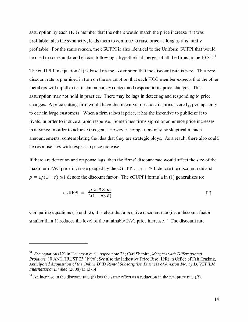
If there are detection and response lags, then the firms’ discount rate would affect the size of the
maximum PAC price increase gauged by the cGUPPI. Let 0 denote the discount rate and
1/ 1 1 denote the discount factor. The cGUPPI formula in (1) generalizes to:
cGUPPI
(2)
Comparing equations (1) and (2), it is clear that a positive discount rate (i.e. a discount factor
smaller than 1) reduces the level of the attainable PAC price increase.35 The discount rate
34 See equation (12) in Hausman et al., supra note 28; Carl Shapiro, Mergers with Differentiated Products, 10 ANTITRUST 23 (1996); See also the Indicative Price Rise (IPR) in Office of Fair Trading, Anticipated Acquisition of the Online DVD Rental Subscription Business of Amazon Inc. by LOVEFiLM International Limited (2008) at 13-14. 35 An increase in the discount rate ( ) has the same effect as a reduction in the recapture rate ( ).
15
creates a financial risk of losing sales if a price increase is not matched. Reducing price provides
a temporary profit increase until the price cut is matched.
To illustrate the cGUPPI calculation, consider as Example 1 a market with four symmetric firms,
in which each firm earns a margin of 36%. Suppose that the diversion ratio to each of the other
firms is 20% and the diversion ratio to outside goods is 40%. Suppose that the HCG consists of
only two firms (so that 36% and 20%). Applying equation (1), the cGUPPI equals
4.5%.36 If the HCG instead were to consist of three firms instead of two, the HCG recapture
rate would increase to 40% and the cGUPPI would rise to 12%.37 If all four firms were
members of the HCG, the cGUPPI would be 27%.38 In this symmetric case, when more firms
are members of the HCG, the cGUPPI is higher. This is because the benefit of a uniform SSNIP
to each firm is higher.
2. Asymmetric Firms
There often are differences among the prices, shares, margins, and diversion ratios of the
products sold by the various firms in the HCG. This asymmetry implies that the various group
members would differ in their “most-preferred” (profit-maximizing) uniform price increases.39
The maximum PAC price increase is determined by the HCG member with the least incentive to
raise price further. We refer to this firm as the “constraining firm” or “constraining member”.
The cGUPPI is then defined as the smallest of the profit-maximizing price increases among the
members of the hypothetical coordinating group, that is, the price increase preferred by the
constraining member.
To illustrate, consider as Example 2 an asymmetric market with four firms. Suppose that firms
A and B each have a 30% share of the market and a margin of 35%. Suppose that firms C and D
36 cGUPPI = 20% x 36% / 2 x (100%-20%) = 7.2%/160% = 4.5%. 37 cGUPPI = 40% x 36% / 2 x (100%-40%) = 14.4%/120% = 12%. 38 cGUPPI =60% x 36% / 2 x (100%-60%) = 21.6%/80% = 27%. 39 See the Appendix for technical details for the situation with zero discount rate. The case of a positive discount rate (and only 2 coordinating firms) is analyzed in our earlier article, Moresi et al., supra note 7.
16
each have a 20% share of the market and each earns a 30% margin. All four firms charge
customers the same price (say, $1 per unit). Customers regard firms A and B as closer
substitutes for each other than for firms C and D, and similarly firms C and D are closer
substitutes for each other than for firms A and B.40
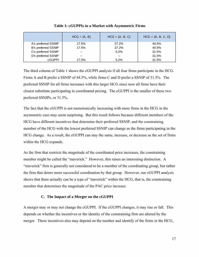
Suppose the HCG is composed only of firms A and B. Given the symmetry between firms A
and B, both prefer the same magnitude SSNIP if they engage in PAC, resulting in a pre-merger
cGUPPI of 17.5%. Firms A and B may gain so much by eliminating competition between one
another than they are willing to lose some sales to firms C and D. This outcome is shown in the
first column of Table 1.
Suppose instead that the HCG is composed of firms A, B, and C, as shown in the second column
of Table 1. With an expanded HCG, the larger firms A and B prefer a larger SSNIP of 27.2%,
since they benefit from firm C also raising its price by the same percentage. However, firm C
prefers a much lower SSNIP of 5.2%. Because firms A and B are not particularly close
substitutes for firm C, firm C does not derive as much benefit from a uniform SSNIP across
firms A, B, and C. Firm C also might be concerned about a sales loss to firm D, whereas firms A
and B may be willing to bear that loss in order to obtain higher prices. But since firm C is the
constraining firm in this case, its preferences rule and the cGUPPI is 5.2%. This is why a larger
HCG need not lead to a higher cGUPPI when the firms are asymmetric.
40 Specifically, we assume that the diversion ratio from each of the four firms to outside goods is 30%. If all four firms were equally close substitutes, the diversion ratio from firm A to firms C and D would be 20% each, while the diversion ratio from A to B would be 30%. In this example, we assume that the diversion ratio from A to each of C and D is half as large (i.e. 10% instead of 20%), while the diversion ratio from A to B is 50% instead of 30%. The diversion ratio from B to A is also 50%, and the diversion ratio from B to each of C and D is also 10%. Turning to firms C and D, we assume that the diversion ratio from C to each of A and B is 14%, while the diversion ratio from C to D is 42%. The diversion ratio from D to C is also 42%, and the diversion ratio from D to each of A and B is also 14%. Formally, these diversion ratios are consistent with a nested logit demand structure, with firms A and B in one nest and firms C and D in another nest, each with a nesting parameter of about 0.417.
17
Table 1: cGUPPIs in a Market with Asymmetric Firms
The third column of Table 1 shows the cGUPPI analysis if all four firms participate in the HCG.
Firms A and B prefer a SSNIP of 44.5%, while firms C and D prefer a SSNIP of 31.5%. The
preferred SSNIP for all firms increases with this larger HCG since now all firms have their
closest substitute participating in coordinated pricing. The cGUPPI is the smaller of these two
preferred SSNIPs, or 31.5%.
The fact that the cGUPPI is not monotonically increasing with more firms in the HCG in the
asymmetric case may seem surprising. But this result follows because different members of the
HCG have different incentives that determine their preferred SSNIP, and the constraining
member of the HCG with the lowest preferred SSNIP can change as the firms participating in the
HCG change. As a result, the cGUPPI can stay the same, increase, or decrease as the set of firms
within the HCG expands.
As the firm that restricts the magnitude of the coordinated price increases, the constraining
member might be called the “maverick.” However, this raises an interesting distinction. A
“maverick” firm is generally not considered to be a member of the coordinating group, but rather
the firm that deters more successful coordination by that group. However, our cGUPPI analysis
shows that there actually can be a type of “maverick” within the HCG, that is, the constraining
member that determines the magnitude of the PAC price increase.
C. The Impact of a Merger on the cGUPPI
A merger may or may not change the cGUPPI. If the cGUPPI changes, it may rise or fall. This
depends on whether the incentives or the identity of the constraining firm are altered by the
merger. These incentives also may depend on the number and identify of the firms in the HCG,
including whether one or both of the merging firms are members of the HCG, and whether the
HCG changes as a result of the merger.41
1. Merger Impact When the HCG Does Not Change
Consider first the symmetric market in Example 1 analyzed above. To isolate the coordinated
effects, assume that the merger would generate a 14% reduction in the marginal costs of the
combined firm, which would imply that there would be no unilateral effects from the merger in
the absence of PAC.42
The impact of the merger on the cGUPPI depends on whether or not one or both of the merging
firms are members of the HCG. Consider initially the scenarios where both merging firms either
were members of the pre-merger HCG, or both were not members. In these scenarios, the HCG
does not change as a result of the merger. If neither of the merging firms were members of the
pre-merger HCG, and the merger generates no unilateral effects (as we assume), then the merger
has no effect on the incentives of the HCG members. As a result, the cGUPPI is unchanged by
the merger, and the Delta cGUPPI is zero.43
In contrast, suppose that the pre-merger HCG is composed solely of the two merging firms, both
before and after the merger. In this case, the cGUPPI is 0% post-merger, and the Delta cGUPPI
is negative. This result follows because the merger effectively allows the merging firms to
41 In this regard, it is not always clear which firms will choose to be members of the HCG; the cGUPPI analysis does not provide an answer to that question. 42 This cost reduction would need to exceed the simple GUPPI because the two merging firms would be raising price simultaneously. Specifically, the cost reduction needed is equal to the compensating marginal cost reduction (CMCR), as explained in equations (A6) and (A7) in the Appendix. In particular, with a 20% diversion ratio between the merging firms and a margin of 36%, the CMCR is about 14%. In the absence of PAC, the cost reduction would raise the margin of the merged firm to 45%, but the market shares, prices and diversion ratios among the four firms, and the margin of non-merging firms, would not be affected by the merger. 43 Note that this result depends on our assumption that members of the HCG take the prices of non-members as given when computing their preferred SSNIP. In the next section, we show that the merger can change the preferred SSNIP of HCG members if non-participants are assumed to make accommodating responses to PAC pricing, even when the merger creates no unilateral effects.
19
coordinate with each other, and the merged firm would maximize the post-merger total profits of
the two brands. Hence, there is no incentive to engage in further coordination through PAC.
The cGUPPI also could fall in a different scenario. Consider the scenario where the pre-merger
HCG includes one or both non-merging firms in addition to the merging firms. In this scenario,
the merger reduces the incentive of the merged firm to coordinate with the other HCG members.
As a result, the Delta cGUPPI is negative in each case and the Delta cGUPPI is equal to -4.5%
regardless of whether the pre-merger HCG consists of 2, 3 or 4 firms. For example, when the
HCG consists of the two merging firms plus one other, the pre-merger cGUPPI is 12%. Post-
merger, the preferred SSNIP of the two merging firms is 7.5%, so the post-merger cGUPPI is
7.5% giving a Delta cGUPPI of -4.5%.
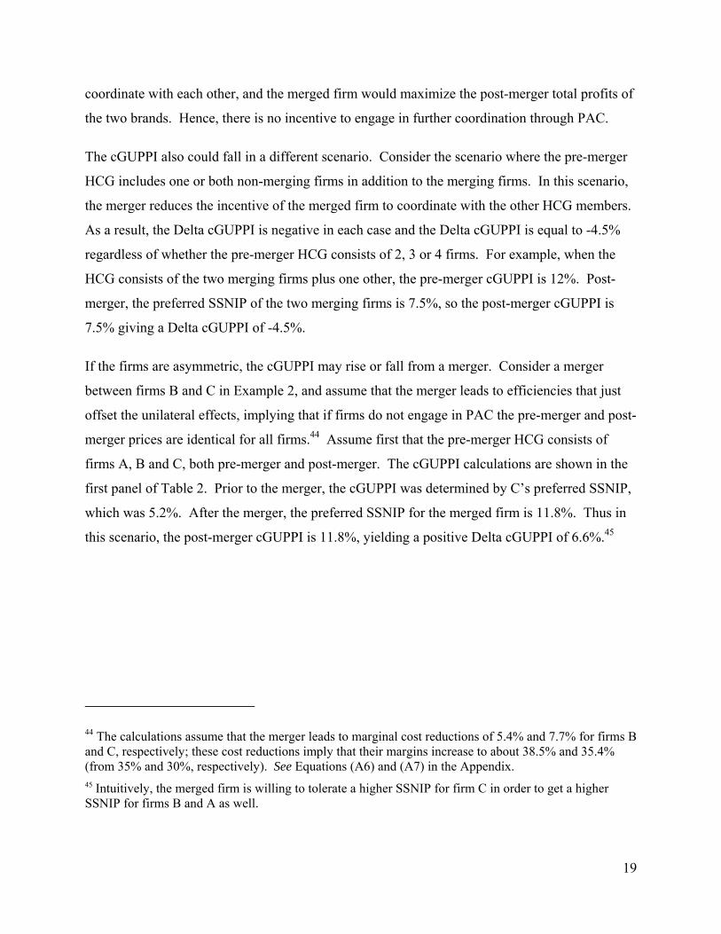
If the firms are asymmetric, the cGUPPI may rise or fall from a merger. Consider a merger
between firms B and C in Example 2, and assume that the merger leads to efficiencies that just
offset the unilateral effects, implying that if firms do not engage in PAC the pre-merger and post-
merger prices are identical for all firms.44 Assume first that the pre-merger HCG consists of
firms A, B and C, both pre-merger and post-merger. The cGUPPI calculations are shown in the
first panel of Table 2. Prior to the merger, the cGUPPI was determined by C’s preferred SSNIP,
which was 5.2%. After the merger, the preferred SSNIP for the merged firm is 11.8%. Thus in
this scenario, the post-merger cGUPPI is 11.8%, yielding a positive Delta cGUPPI of 6.6%.45
44 The calculations assume that the merger leads to marginal cost reductions of 5.4% and 7.7% for firms B and C, respectively; these cost reductions imply that their margins increase to about 38.5% and 35.4% (from 35% and 30%, respectively). See Equations (A6) and (A7) in the Appendix. 45 Intuitively, the merged firm is willing to tolerate a higher SSNIP for firm C in order to get a higher SSNIP for firms B and A as well.
20
Table 2: Impact of a Merger in a Market with Asymmetric Firms
2. Merger Impact When the HCG Participation Changes
A merger can change the composition of the HCG itself. For example, this might occur when
the merger combines a firm that was a member of the pre-merger HCG with a firm that was not a
member. There are two contrasting scenarios here, depending on whether the merged firm
remains a member of the HCG and “eliminates the maverick,” or whether the merged firm drops
out of the HCG and becomes a “super-maverick.” In either case, the cGUPPI can increase or
decrease following the merger, depending on the details of the market structure.
To see this result when a merger expands the HCG, consider first the symmetric market in
Example 1 above, with two firms in the pre-merger HCG and a pre-merger cGUPPI of 4.5%.
Now suppose one of the HCG members merges with a non-participant, and the merged firm
remains a member of the HCG. As discussed previously, the cGUPPI in this case (with a HCG
consisting of the merged firm and one other) is 7.5%. Thus the Delta cGUPPI is 3%. In this
scenario, the merger would increase PAC concerns. This corresponds to the case of the merger
eliminating a maverick (i.e. reducing the pricing constraints from firms outside the HCG).
Consider Example 2 next, assuming a pre-merger HCG of firms A and B. Suppose that firms B
and C merge and C joins the HCG. As shown in the second panel of Table 2, the pre-merger
cGUPPI is 17.5%. The post-merger cGUPPI with firms A, B and C all in the HCG is 11.8%.
Thus the cGUPPI falls, with a Delta cGUPPI of -5.7%. In this scenario, a merger that brings the
merging partner into the HCG counterintuitively would reduce the likelihood of PAC, despite the
fact that the size of the HCG increases. This is because the new member of the HCG (i.e. firm
C) prefers a much smaller PAC price increase than the other members (i.e. firms A and B). The
merger still reduces the pricing constraints from outside the HCG, but it increases the constraints
from inside the HCG by even more.46
Alternatively, suppose a firm in the HCG merges with a non-participant, and the merged firm
drops out of the post-merger HCG. With the symmetric firms in Example 1, the impact can be
determined directly from the cGUPPIs reported previously. A pre-merger HCG with three firms
has a cGUPPI of 12%. After the merger, only two (non-merged) firms are left in the HCG, so
the cGUPPI is 4.5%. Thus, the cGUPPI falls as a result of the merger, with a Delta cGUPPI of
−7.5%. This corresponds to the scenario of the creation of a super-maverick.
However, a merger that results in a firm withdrawing from the HCG counterintuitively can have
the opposite effect on PAC concerns in a market that is initially asymmetric. The third panel of
Table 2 shows the impact of a merger between firms C and D when the initial HCG was
comprised of firms A, B, and C, and the merger leads to firm C exiting the post-merger HCG.
The cGUPPI rises from 5.2% pre-merger to 17.5% post-merger, giving a Delta cGUPPI of
12.3%. In this example, even though the size of the HCG is reduced, the remaining HCG firms
counterintuitively are more likely to engage in PAC. This is because the merger eliminates the
pricing constraint inside the HCG.
This raises the interesting question of which scenario is more likely, that is, which firms are more
likely to be members of the HCG and which products will they target for a PAC price increase. 46 A theoretical possibility might involve the merged firm retaining member brand (B) inside the HCG but retaining the non-member brand (C) outside the HCG. This raises the question of why the merged firm would engage in PAC with only one of its brands as opposed to both brands. The reasoning can be explained with a hypothetical example. Suppose hypothetically that The Coca-Cola Company were to acquire the Perrier brand (from Nestlé Corporation). It conceivably might decide not to raise the price of Perrier when engaging in PAC with PepsiCo over cola-flavored carbonated soft drinks. In this scenario, the merger would have no effect on the cGUPPI, and the Delta cGUPPI would be zero. The merger does increase the incentive of the merged firm to engage in PAC because the non-member brand (Perrier – firm C in the text) benefits from the PAC price increase of the non-merging firm (Pepsi -- firm A in the text). However, the cGUPPI does not increase because the merged firm is not the constraining member of the HCG. The post-merger cGUPPI instead is determined by the preferred SSNIP of other member of the HCG, which does not change from the merger. In contrast, if Perrier were to join the HCG, competition it faces from other non-cola brands might constrain the PAC price increase.
22
The simple cGUPPI analysis unfortunately cannot answer this question. The incentives of
whether or not to join the HCG involve a number of factors that are not captured by the cGUPPI.
These include the degree of information that affects monitoring costs and effectiveness, and
detection lags, and the level of the firm’s discount rate. For this reason, the cGUPPI provides
only an initial score, while raising additional issues for investigation.
In summary, the Delta cGUPPI resulting from a merger depends on the interaction between a
number of considerations: whether the merging firms were HCG members prior to the merger
and whether they will remain in the HCG post-merger, which firm was the constraining firm pre-
merger, and whether the incentives of the merging firms to engage in PAC change, resulting
from both recaptured diversion between the two firms and merger efficiencies. A merger can
lead to a positive, negative or zero Delta cGUPPI, whether or not the merger brings an additional
brand into the HCG. This indicates that every merger that raises PAC issues requires its own
cGUPPI analysis to discern the possible impact on PAC incentives. It also means that the
cGUPPI requires careful market analysis regarding the likely HCG.
IV. Comparison of the cGUPPI and Simulation Methodologies
We previously explained two key assumptions of the cGUPPI methodology. First, the cGUPPI
evaluates PAC pricing incentives while holding the prices of non-coordinating firms constant at
the pre-merger level. The cGUPPI thus does not take into account the potential pricing
responses from non-coordinating firms, including any feedback effects on the PAC price
increase of the coordinating firms. Second, the post-merger cGUPPI evaluates PAC pricing
incentives while assuming that the merger creates no unilateral effects. The cGUPPI is premised
on the merging firms having an “efficiency credit” equal to the CMCRs. These two assumptions
permit the definition of a simple cGUPPI metric to evaluate coordinated effects concerns,
separately from unilateral effects concerns and without the need for simulation models.
In this section, we discuss the potential biases that might be created by these two assumptions.
We frame our analysis in the context of the same hypothetical market analyzed in Example 2,
involving a merger of two firms in a fictitious market with four asymmetric firms (A, B, C and
D). We then analyze the equilibria in two related simulation models that capture the added
23
complexity of accounting for unilateral effects and the pricing responses of rivals. This permits a
comparison of the cGUPPI score to the full PAC equilibrium.
We first apply a standard merger simulation model to predict the post-merger unilateral effects
equilibrium price increases when efficiencies differ from the CMCRs.47 Starting from this
equilibrium, we then apply a PAC simulation model to derive the “full PAC equilibrium” that
takes into account the pricing responses by non-coordinating firms. We similarly apply this PAC
simulation model to the initial pre-merger equilibrium, and then compare the full pre- and post-
merger PAC equilibria. This comparison suggests that the Delta cGUPPI score is a fairly good
approximation for the impact of a merger on the full PAC equilibrium.
A. Accounting for Actual Efficiencies and Unilateral Effects
Before examining the full PAC equilibrium (including pricing responses from firms not in the
HCG) we first analyze the impact of merger-specific marginal cost reductions on the cGUPPI
and Delta cGUPPI computations. We focus on the merger between firms B and C in Example 2,
which was introduced in the previous section.48
Table 3 shows the unilateral effects arising under three assumptions about the magnitude of
efficiencies: no efficiencies, efficiencies equal to the CMCRS, and efficiencies equal to 150% of
the CMCRs. With no efficiencies, the equilibrium unilateral price increase (EUPI) for firms B
and C are 2.0% and 2.9%, respectively, while the non-merging firms respond by raising prices
less than 1%. The CMCRs that exactly counterbalance the upward pricing pressure from the
merger are 5.4% and 7.7% for firms B and C, respectively. When efficiencies equal 150% of the
CMCRs, the EUPI shows a price decrease, with the magnitude of the price changes equal to half
of the price increases under the no efficiencies scenario.
47 As noted in the Merger Guidelines at §6.1, “Where sufficient data are available, the Agencies may construct economic models designed to quantify the unilateral price effects resulting from the merger. These models often include independent price responses by non-merging firms. They also can incorporate merger-specific efficiencies.” 48 The results for the other merger scenarios we have examined are comparable.
24
Table 3: Efficiencies and Unilateral Effects from a Merger of Firms B and C
We next compute the PAC equilibrium for the various efficiency scenarios. We focus on the
case where both the pre-merger and post-merger HCG is composed of firms A, B, and C.49
Table 4 shows the cGUPPIs before and after a merger between firms B and C under the three
different assumptions about the cost reductions from the merger.50
Table 4: Impact of a Merger of B and C on PAC Incentives
When there are no efficiencies from the merger, the starting point involves the post-merger non-
cooperative equilibrium prices for the merged firm, which are 2% to 3% higher than pre-merger
prices, as shown in Table 3. The post-merger cGUPPI here (as determined by the preferred
SSNIP of the merged firm) is 10.7%., which is less than the cGUPPI of 11.8% when efficiencies
49 The other case discussed in the previous section, with a pre-merger HCG composed of firms A and B, leads to similar conclusions about the impact of the efficiency and non-participant response assumptions discussed in this section. 50 The pre-merger and post-merger cGUPPIs shown here for the case of efficiencies equal to the CMCRs reproduce the cGUPPIs reported in Table 2.
Post-merger Efficiencies (% of CMCR)HCG = {A, B, C}
25
equal the CMCRs.51 Because the starting point involves higher prices, the PAC equilibrium with
no efficiencies actually results in higher prices than when efficiencies are equal to the CMCRs,
despite the fact that the cGUPPI is lower. Because the cGUPPI is lower with smaller post-
merger efficiencies, the Delta cGUPPI also is lower, 5.5% versus 6.6% when efficiencies equal
the CMCRs.
These results all move in the opposite direction when merger efficiencies are larger than the
CMCRs. The merging firms prefer larger post-merger PAC price increases (12.3% versus
11.8%). This leads to a higher post-merger cGUPPI and Delta cGUPPI (7.1% versus 6.6%).
These results occur despite the fact that the post-merger price of the merging firm resulting from
the combination of unilateral effects and PAC is lower than when efficiencies equal the CMCRs.
These results indicate that, while the post-merger cGUPPIs and Delta cGUPPIs vary with the
level of efficiencies, they do so in intuitive and predictable ways. After taking the actual
efficiencies into account, the Delta cGUPPIs remain within one percentage point of the results
when it is assumed that the efficiencies are equal to the CMCRs. Thus, the inferences drawn
from the Delta cGUPPI on the impact of a merger are a fairly close approximation, despite
significantly different efficiencies.
B. Accounting for Pricing Responses by Non-coordinating Firms
The pre-merger cGUPPI of 5.2% in Table 4 means that, if firms A, B and C were to engage in
PAC, they would have an incentive to raise price by 5.2%, holding the price of firm D constant.
This raises the question of how the pricing responses by non-coordinating firms would affect
PAC price increases, both before and after a merger. It also raises a question of whether these
pricing responses would significantly affect the Delta cGUPPI.
We analyze this issue by applying a simulation model to determine the equilibrium market prices
following a successful PAC price increase. When an HCG of firms A, B and C engage in PAC
pricing, firm D benefits because some customers of the other firms will substitute to firm D
51 Conversely, the preferred SSNIP for firm A is higher when then are no efficiencies from the merger.
26
following the price increase. Given this increase in demand, firm D’s profit-maximizing best
response is to raise its own price moderately, so as to increase both its margin and output.52
Because the firms in the HCG can anticipate this “partially accommodating” response by firm D,
their own incentives to raise price through PAC tend to be stronger, relative to the cGUPPI that
assumed no pricing response by HCG non- members.53 This can be seen by comparing Tables 4
and 5.
Table 5: Impact of a Merger of B and C on PAC Incentives Accounting for Pricing Responses by Firms Outside the HCG
52 An implication of the Bertrand price competition model (where firms sell imperfect substitutes) is that all firms have incentives to raise their prices in response to a price increase by competing firms. Non-coordinating firms generally respond with price increases that are smaller than the uniform SSNIP of the coordinating firms. 53 The PAC simulation model used in this version of the paper is a static Nash equilibrium model involving the HCG and the non-coordinating firms, starting from the pre-merger unilateral (non-PAC) equilibrium. Specifically, the HCG and the non-coordinating firms set prices simultaneously. The HCG sets a uniform price increase above the unilateral equilibrium prices of the HCG members, taking the PAC equilibrium prices of the non-coordinating firms as given. Each of the non-coordinating firms sets a price increase above its unilateral equilibrium price, taking the PAC equilibrium prices of the HCG members as given. The "full PAC equilibrium" is the Nash equilibrium of this game. An interesting alternative might be to analyze a dynamic Stackelberg model, starting from the same unilateral equilibrium outcome. In this model, the HCG would be the "Stackelberg leader" and the non-coordinating firms would be the "Stackelberg followers." The HCG thus would anticipate and take into account the pricing responses of non-coordinating firms, while the latter would take the prices of the HCG members as given. In preliminary work with this model, it appears that the Stackelberg model produces Delta cGUPPIs that are similar to the Nash model.
Pre-merger0% 100% 150%
PAC EPI for A 5.7% 11.6% 12.7% 13.4%PAC EPI for B 5.7% 11.6% 12.7% 13.4%PAC EPI for C 5.7% 11.6% 12.7% 13.4%PAC EPI for D 1.9% 4.0% 4.3% 4.5%
Post-merger Efficiencies (% of CMCR)HCG = {A, B, C}
27
Comparing the first column of Table 5 with the corresponding column in Table 4, the pre-merger
PAC equilibrium price increase is equal to 5.7%, as opposed to 5.2% when the price of firm D
was assumed to be held constant. In the pre-merger PAC equilibrium, firm D raises its price by
1.9%. Table 5 also shows that a similar effect occurs after the merger of firms B and C. For
example, when the merger generates efficiencies equal to the CMCRs, the post-merger PAC
equilibrium price increase is 12.7%, as opposed to 11.8% in the corresponding column of
Table 4 (when the price of firm D is held constant).
The Delta cGUPPI computations in Table 5 reflect the increases in the cGUPPI after accounting
for accommodating responses from firms outside the HCG. The results differ from the Delta
cGUPPIs in Table 4. However, the pre- and post-merger increases in the cGUPPI largely offset
one another, resulting in relatively small changes in the computed Delta cGUPPIs. The third
column of Table 4 (efficiencies equal to CMCRs) shows the Delta cGUPPI of 6.6% when
holding the price of non-participating firms constant. After accounting for accommodating
responses of all firms using a PAC simulation model, the Delta cGUPPI in the corresponding
column of Table 5 is 7.0%. The 0.4% difference shown in the bottom row of the table is very
small. The change in the Delta cGUPPI from using the simulation model is no more than 0.5
percentage points in all the scenarios in Table 5.
These results suggest that accounting for pricing responses by non-coordinating firms also is
unlikely to have a significant effect on the predicted likely impact of a merger on PAC
incentives. While it is the case that pricing feedback effects between coordinating and non-
coordinating firms generally lead to PAC price increases that are higher than the cGUPPIs, this
effect occurs both pre- and post-merger. As a result, the Delta cGUPPI score captures
reasonably well the likely impact of the merger. Of course, this conclusion still should be
regarded as somewhat preliminary until it is confirmed in a wider range of merger settings.
V. Conclusions
The cGUPPI metric formulated in this article is another incentive scoring device for evaluating
the potential competitive effects of mergers. Unlike some other indices, the cGUPPI has the
advantage of being based on profit-maximizing incentives. The cGUPPI scores the incentives of
firms to engage in parallel accommodating conduct, where that PAC is implemented as a
28
uniform percentage price increase by the coordinating firms. The merger-induced change in that
cGUPPI (the Delta cGUPPI) is a signal of the extent to which those PAC incentives change as a
result of the merger.
While the cGUPPI is a useful screen, it is not intended to provide a complete analysis. The Delta
cGUPPI may be distorted when there is PAC in the pre-merger market. The cGUPPI by itself
does not explain the identity of the coordinating firms, nor how the coordinating firms chose
which product(s) to target for a PAC price increase. Nor can the cGUPPI explain by itself how
the merger might change the identity of the coordinating firms. The formulation of the simple
cGUPPI in this article also does not take into account all the impediments to PAC and other
forms of coordination or how the merger might change those impediments. Those factors all
must be evaluated separately. Once they are, they can be incorporated into a refined cGUPPI
measure or combined less formally into a more complete analysis.
However, these complexities do not devalue the insights that follow from cGUPPI analysis. The
cGUPPI furthers our understanding of the competitive interaction involved in PAC. The ways in
which the various complicating elements arise in that interaction, and some counterintuitive
results that follow from them, are well highlighted by the cGUPPI analysis. And despite these
complexities, the cGUPPI also remains a helpful starting point. We also recognize (and hope)
that this article is not the final work on the topic, and we have suggested some way to
incorporate these complicating factors in further analysis. Our hope is that this initial cGUPPI
analysis will provide a stepping stone to a deeper understanding of these important competition
issues.
29
Appendix
We consider the standard framework of Bertrand price competition with differentiated products.
To allow for multi-product firms, we distinguish between firms and products (or brands) and we
denote by iB the set of products sold by firm i. We use jP , jC , and mj= ⁄ to
denote the price, marginal cost, sales volume, and percentage margin of brand j , respectively.
Moreover, jk denotes the diversion ratio from brand j to brand k .54 One can show that firm
i’s first-order conditions of profit-maximization imply that the own-price elasticity of demand for
any product j sold by the firm (which we denote j ) satisfies the following equation:55
iBk
jkkjkj
PPm /1
(A1)
Starting from the Bertrand-Nash equilibrium as the initial status quo, suppose that the owners of
a collection of M brands were to coordinate and raise the prices of these M brands by the same
percentage amount, s . (In the antitrust jargon, s is commonly referred to as a uniform SSNIP.)
Thus, the price of each of these M brands would increase from jP to jPs)1( . Note that the M
brands subject to the coordinated price increase may not include all the brands sold by the
would-be coordinating firms. For example, if each of the would-be coordinating firms owns a
premium and a value brand, coordination may involve only the prices of the firms’ premium
brands. For this reason, it is convenient to assume that each would-be coordinating firm owns
brands that are subject to the SSNIP and brands that are not subject to the SSNIP (i.e.
∪ ). We refer to the would-be coordinating firms as the “hypothetical coordinating
group” (HCG) and to the M brands subject to the SSNIP as the “targeted coordinating brands”.
54 For all j and k,
⁄
⁄ where and denote the demand functions of brands j and k,
respectively. 55 (A1) is evaluated at the Nash equilibrium point. See Moresi et al., supra note 1.
30
If there is no prior understanding leading to the PAC equilibrium, it is reasonable to assume that
such equilibrium would have to be individually rational for each participant, without relying on
transfer payments from one firm to another. The PAC equilibrium price increase, s*, would be
such that at least one participating firm would not be willing to match a further price increase
even assuming that all the other would-be coordinating firms would match that further increase.
A particularly relevant model of PAC is found in Lu and Wright (2010).56 They focus on the
case with symmetric single-product firms, while we consider asymmetric multi-product firms.
To simplify the dynamics of the model and derive relatively simple formulas, we assume that
firms are very patient (or equivalently the length of a period and the detection lag are very short).
Consider the incentives of a single firm k to match a PAC price increase of s relative to
maintaining the non-cooperative equilibrium price level. The break-even SSNIP for firm k,
denoted , is such that the total profits for all brands owned by firm k are the same before and
after all firms in the HCG raise the prices of all targeted products by , and satisfies57
kkk Niii
Mjjjji
BEki
Mii
Mjjjji
BEki
BEki
Biiii PmQsQPQsQsmPmQ )())(( (A2)
The left hand side of (A2) is firm k’s profit before implementation of PAC. The right hand side
is the profit of firm k after the prices of all targeted coordinating brands are increased by .
The first summation is for firm k’s targeted brands while the second is for firm k’s other brands.
In both summations, the quantity term is the original quantity plus the net change after diversion
from all targeted coordinating brands following the SSNIP.58 The quantity term is multiplied by
the dollar margin, which for targeted coordinating brands is augmented by the SSNIP.
56 See supra note 13. For symmetric firms, the cGUPPI coincides with the (limit) highest PAC price that can be sustained in their model when firms have zero discount rates or when detection lags are very short. 57 We are assuming linear demand and that the resulting quantities following the SSNIP are non-negative. 58 The net change in quantity is positive for brands not subject to the SSNIP. For a targeted coordinating brand, the net change in quantity is typically negative, although it can be positive if the diversion to the brand (from other brands raising their prices is greater than the loss in sales from raising its own price.
31
Solving for ,
k
kk
Mi Mjjjjii
Bi Mjjjjiii
Miii
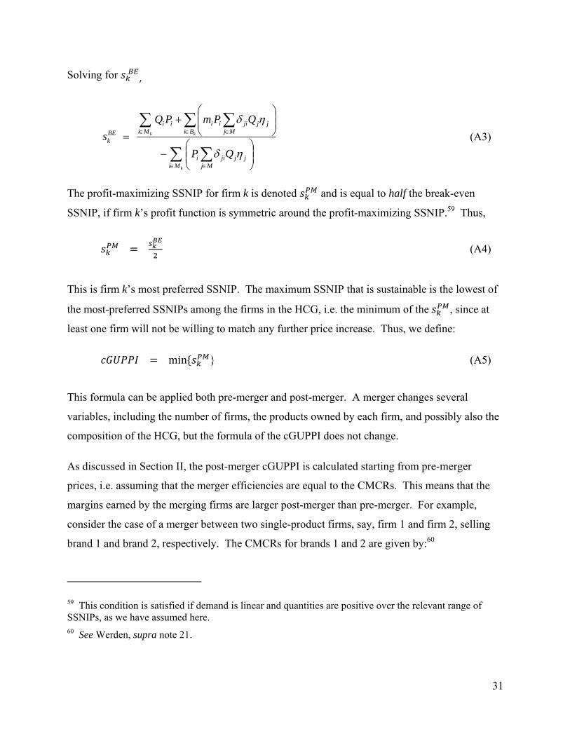
BEk
QP
QPmPQ
s
(A3)
The profit-maximizing SSNIP for firm k is denoted and is equal to half the break-even
SSNIP, if firm k’s profit function is symmetric around the profit-maximizing SSNIP.59 Thus,
(A4)
This is firm k’s most preferred SSNIP. The maximum SSNIP that is sustainable is the lowest of
the most-preferred SSNIPs among the firms in the HCG, i.e. the minimum of the , since at
least one firm will not be willing to match any further price increase. Thus, we define:
min } (A5)
This formula can be applied both pre-merger and post-merger. A merger changes several
variables, including the number of firms, the products owned by each firm, and possibly also the
composition of the HCG, but the formula of the cGUPPI does not change.
As discussed in Section II, the post-merger cGUPPI is calculated starting from pre-merger
prices, i.e. assuming that the merger efficiencies are equal to the CMCRs. This means that the
margins earned by the merging firms are larger post-merger than pre-merger. For example,
consider the case of a merger between two single-product firms, say, firm 1 and firm 2, selling
brand 1 and brand 2, respectively. The CMCRs for brands 1 and 2 are given by:60
59 This condition is satisfied if demand is linear and quantities are positive over the relevant range of SSNIPs, as we have assumed here. 60 See Werden, supra note 21.
32
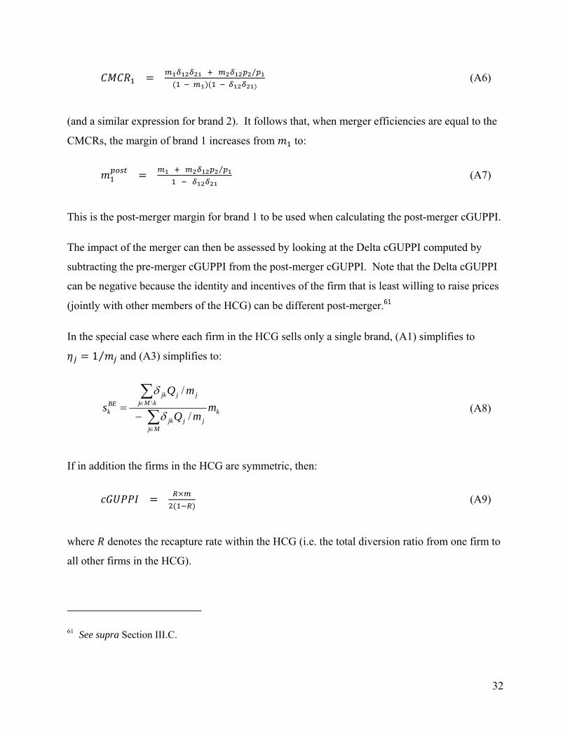
⁄
(A6)
(and a similar expression for brand 2). It follows that, when merger efficiencies are equal to the
CMCRs, the margin of brand 1 increases from to:
⁄
(A7)
This is the post-merger margin for brand 1 to be used when calculating the post-merger cGUPPI.
The impact of the merger can then be assessed by looking at the Delta cGUPPI computed by
subtracting the pre-merger cGUPPI from the post-merger cGUPPI. Note that the Delta cGUPPI
can be negative because the identity and incentives of the firm that is least willing to raise prices
(jointly with other members of the HCG) can be different post-merger.61
In the special case where each firm in the HCG sells only a single brand, (A1) simplifies to
1⁄ and (A3) simplifies to:
k
Mjjjjk
kMjjjjk
BEk m
mQ
mQ
s
/
/\
(A8)
If in addition the firms in the HCG are symmetric, then:
(A9)
where denotes the recapture rate within the HCG (i.e. the total diversion ratio from one firm to