Ch. 1: Data and Distributions • Populations vs. Samples • How to graphically display data – Histograms , dot plots, stem plots, etc – Helps to show how samples are distributed • Distributions of both continuous and discrete variables – Density functions and Mass functions • Three basic properties – Shows the distribution of the entire population or process • Some important distributions and associated Probability – Continuous: Exponential, Normal, Uniform … – Discrete: Binomial, Poisson … 4/24/12 1 H.X. Lecture 30: Final Summary
Transcript
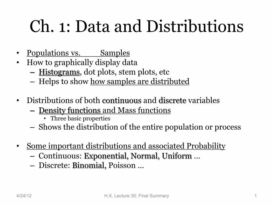
Ch. 1: Data and Distributions • Populations vs. Samples • How to graphically display data
– Histograms, dot plots, stem plots, etc – Helps to show how samples are distributed
• Distributions of both continuous and discrete variables – Density functions and Mass functions
• Three basic properties – Shows the distribution of the entire population or process
• Some important distributions and associated Probability – Continuous: Exponential, Normal, Uniform … – Discrete: Binomial, Poisson …
4/24/12 1 H.X. Lecture 30: Final Summary
Ch. 2: Numerical Summary Measures
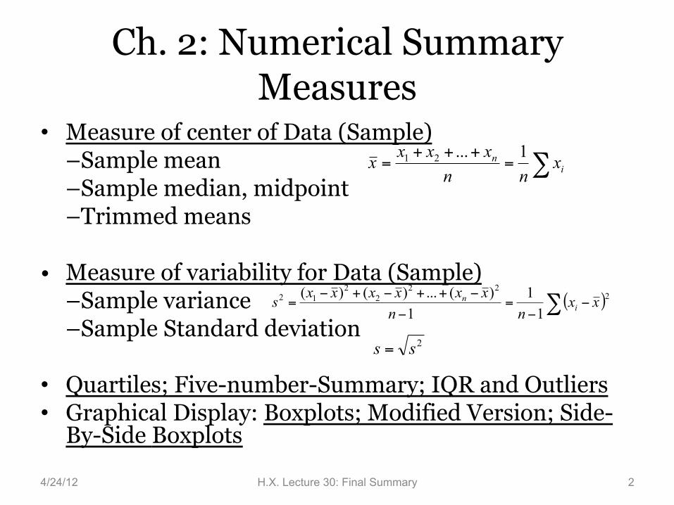
• Measure of center of Data (Sample) –Sample mean –Sample median, midpoint –Trimmed means
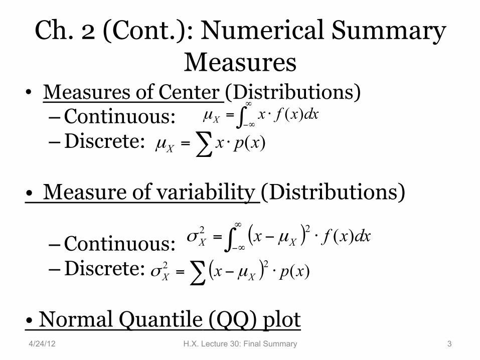
• Measures of Center (Distributions) – Continuous: – Discrete:
• Measure of variability (Distributions)
– Continuous: – Discrete:
• Normal Quantile (QQ) plot
∫∞
∞−⋅= dxxfxX )(µ
∑ ⋅= )(xpxXµ
( )∫∞
∞−⋅−= dxxfx XX )(22 µσ
( )∑ ⋅−= )(22 xpx XX µσ
4/24/12 3 H.X. Lecture 30: Final Summary
Ch.3: Bivariate Data • Scatterplots: Visually Display Bivariate data, y vs. x • Pearson’s Correlation Coefficient (between X and Y, both
quantitative), r : – r measures the strength and direction of the linear
relationship – , other convenient formulas for Sxy, Sxx and Syy
– Takes values between -1 and 1, inclusive • Sign indicates type/direction of relationship (positive, negative) • Value indicates strength: farther from 0 is stronger
– If switch roles of X and Y à r doesn’t change – Unit free—unaffected by linear transformations – Affected by Outliers, Not a resistant measure – Correlation ≠ Causaiton
4/24/12 H.X. Lecture 30: Final Summary 4
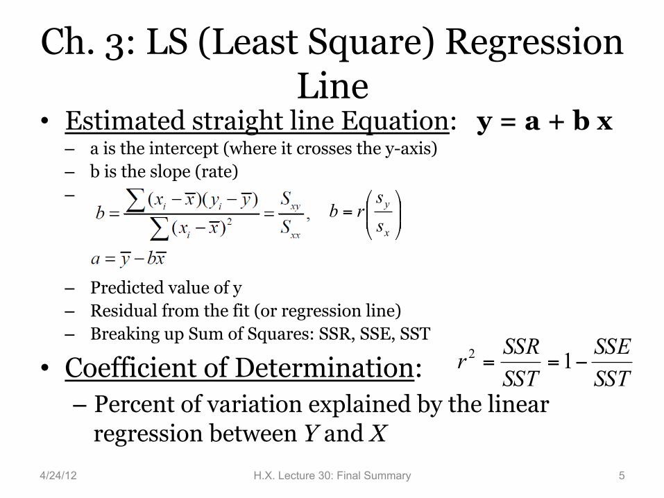
Ch. 3: LS (Least Square) Regression Line
• Estimated straight line Equation: y = a + b x – a is the intercept (where it crosses the y-axis) – b is the slope (rate) –
– Predicted value of y – Residual from the fit (or regression line) – Breaking up Sum of Squares: SSR, SSE, SST
• Coefficient of Determination: – Percent of variation explained by the linear
regression between Y and X
4/24/12 H.X. Lecture 30: Final Summary 5
⎟⎟⎠
⎞⎜⎜⎝
⎛=
x
y
ss
rb
SSTSSE
SSTSSRr −== 12
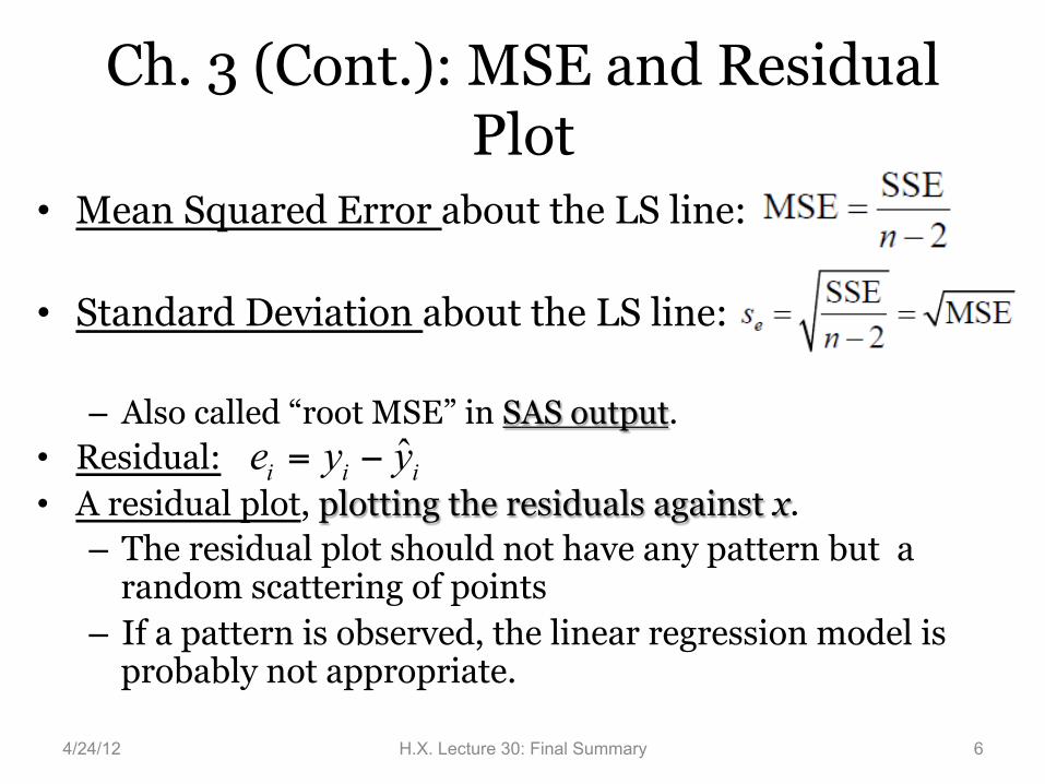
Ch. 3 (Cont.): MSE and Residual Plot
• Mean Squared Error about the LS line:
• Standard Deviation about the LS line:
– Also called “root MSE” in SAS output. • Residual: • A residual plot, plotting the residuals against x.
– The residual plot should not have any pattern but a random scattering of points
– If a pattern is observed, the linear regression model is probably not appropriate.
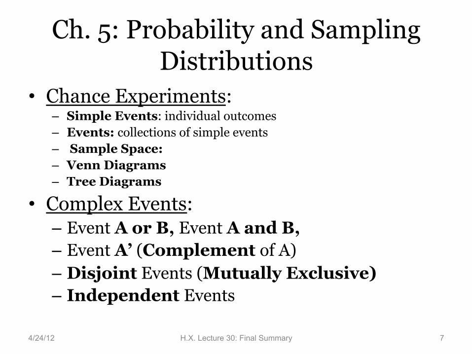
• Complex Events: – Event A or B, Event A and B, – Event A’ (Complement of A) – Disjoint Events (Mutually Exclusive) – Independent Events
4/24/12 H.X. Lecture 30: Final Summary 7
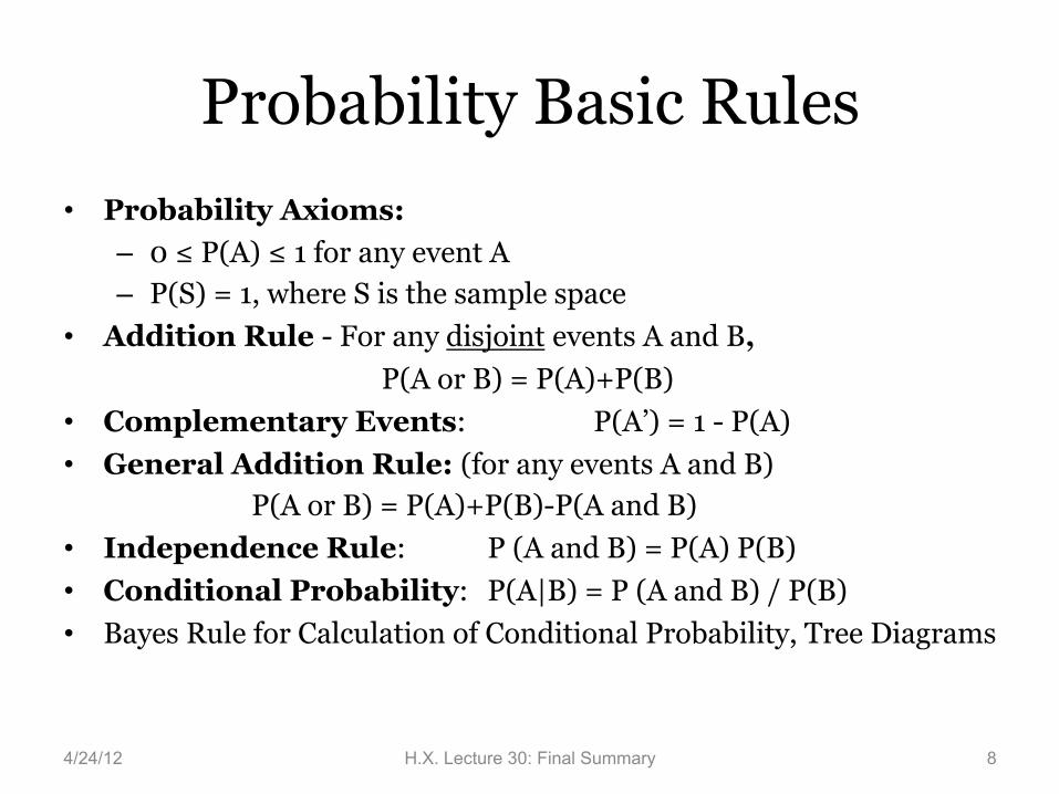
Probability Basic Rules • Probability Axioms:
– 0 ≤ P(A) ≤ 1 for any event A – P(S) = 1, where S is the sample space
• Addition Rule - For any disjoint events A and B, P(A or B) = P(A)+P(B)
• Complementary Events: P(A’) = 1 - P(A) • General Addition Rule: (for any events A and B)
P(A or B) = P(A)+P(B)-P(A and B) • Independence Rule: P (A and B) = P(A) P(B) • Conditional Probability: P(A|B) = P (A and B) / P(B) • Bayes Rule for Calculation of Conditional Probability, Tree Diagrams
4/24/12 H.X. Lecture 30: Final Summary 8
Random Variables and Sampling Distribution
• Random Variables – Discrete Distribution Table, Prob. Histogram – Continuous Distribution Curve, density function – Independent R.V.s
• Sampling Distribution of a Sample Mean • Sampling Distribution of a Sample Proportion
(rule of thumb for Normal Appox.) • Central Limit Theorem • Continuity Correction (from Binomial to Normal
Appox.)
4/24/12 H.X. Lecture 30: Final Summary 9
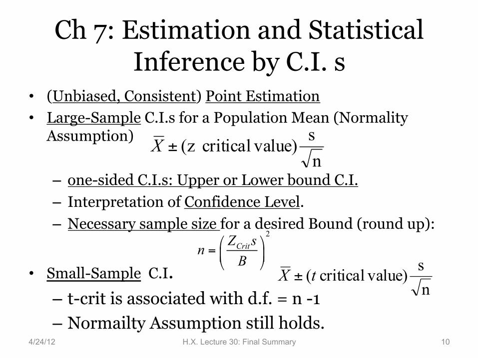
Ch 7: Estimation and Statistical Inference by C.I. s
• (Unbiased, Consistent) Point Estimation • Large-Sample C.I.s for a Population Mean (Normality
Assumption)
– one-sided C.I.s: Upper or Lower bound C.I. – Interpretation of Confidence Level. – Necessary sample size for a desired Bound (round up):
• Small-Sample C.I. – t-crit is associated with d.f. = n -1 – Normailty Assumption still holds.
4/24/12 H.X. Lecture 30: Final Summary 10
ns value)critical (z ±X
2CritZ snB
⎛ ⎞= ⎜ ⎟⎝ ⎠
ns value)critical ( tX ±
C.I. for a Population Proportion • Point Estimation for a Population Proportion • Large-Sample C.I.s for a Population Proportion
– Necessary sample size for a desired Bound (round up for not-an-integer):
• , or 0.5 if p-hat is unavailable.
• Small-Sample C.I. replaces z-crit by t-crit
4/24/12 H.X. Lecture 30: Final Summary 11
ˆ ˆ(1 )ˆ p pp Zcritn−
±
2_*(1 *) z criticaln p pB
⎛ ⎞= − ⎜ ⎟⎝ ⎠
ˆ*p p=
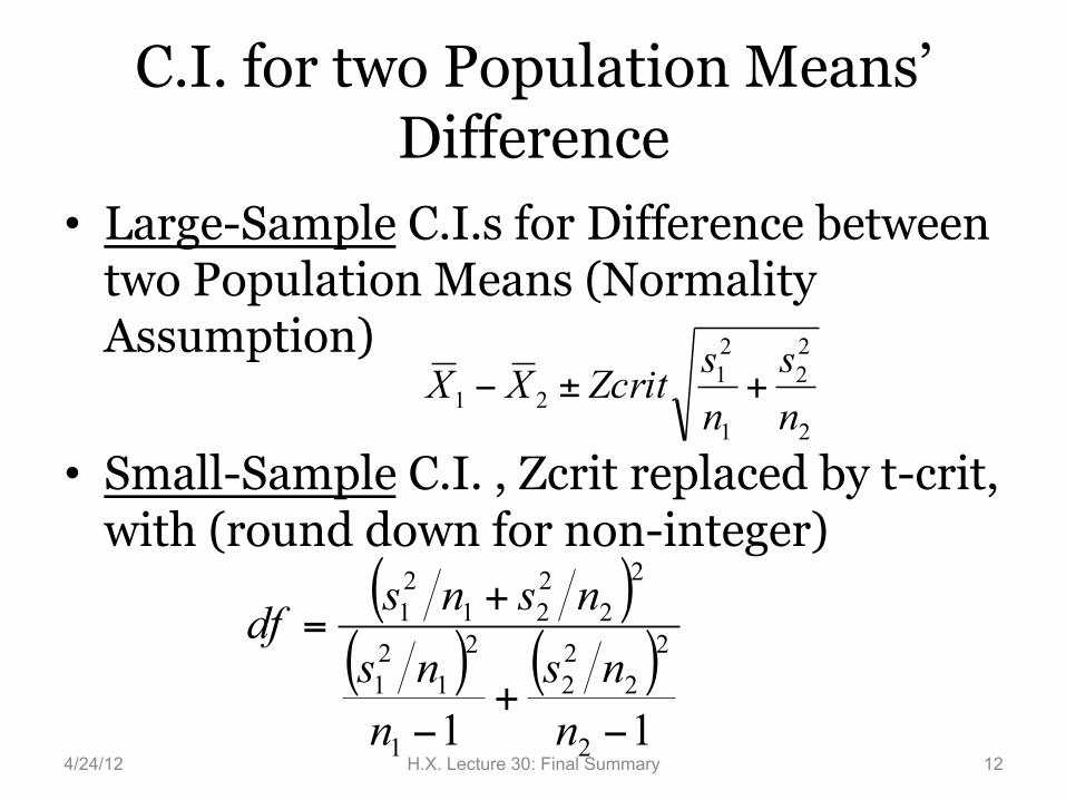
C.I. for two Population Means’ Difference
• Large-Sample C.I.s for Difference between two Population Means (Normality Assumption)
• Small-Sample C.I. , Zcrit replaced by t-crit, with (round down for non-integer)
4/24/12 H.X. Lecture 30: Final Summary 12
2
22
1
21
21 ns
nsZcritXX +±−
( )( ) ( )
11 2
22
22
1
21
21
22
221
21
−+
−
+=
nns
nns
nsnsdf
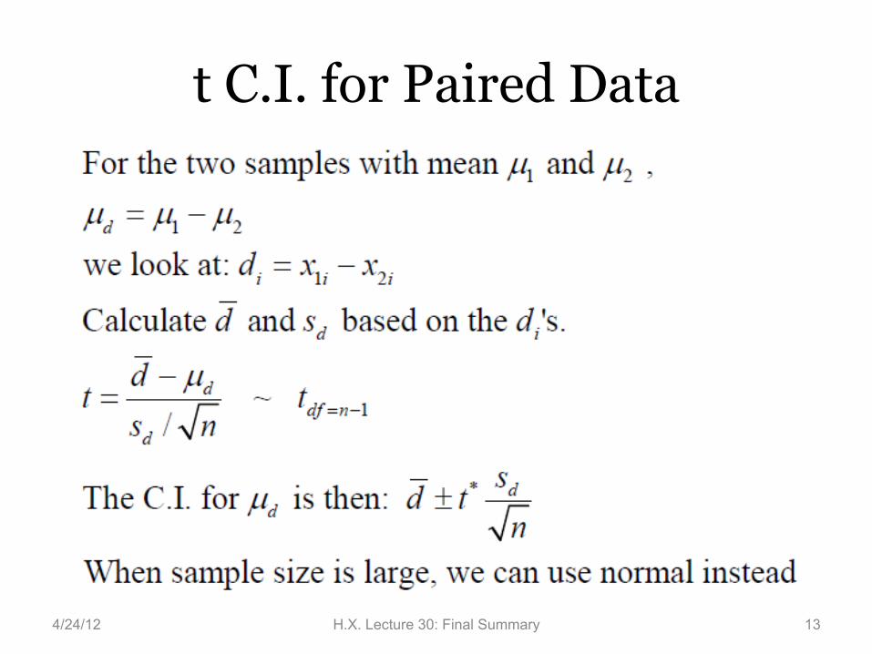
t C.I. for Paired Data
4/24/12 H.X. Lecture 30: Final Summary 13
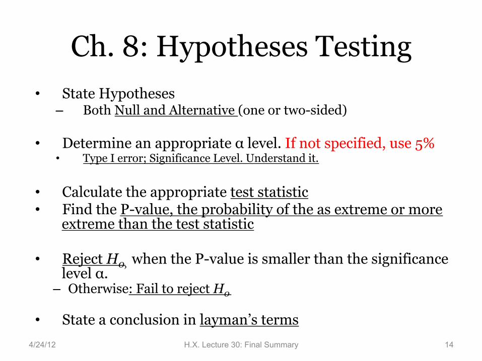
Ch. 8: Hypotheses Testing • State Hypotheses
– Both Null and Alternative (one or two-sided)
• Determine an appropriate α level. If not specified, use 5% • Type I error; Significance Level. Understand it.
• Calculate the appropriate test statistic • Find the P-value, the probability of the as extreme or more
extreme than the test statistic • Reject H0, when the P-value is smaller than the significance
level α. – Otherwise: Fail to reject H0
• State a conclusion in layman’s terms
4/24/12 H.X. Lecture 30: Final Summary 14
One-sample t Test for a Population Mean: • The null hypothesis is H0: µ = µ0 • The alternative hypothesis could be:
• If n is large (≥30), CLT guarantees an approximate normal
distribution and the t can be replaced with z, where z follows a standard normal distribution.
nsXt 0µ−=
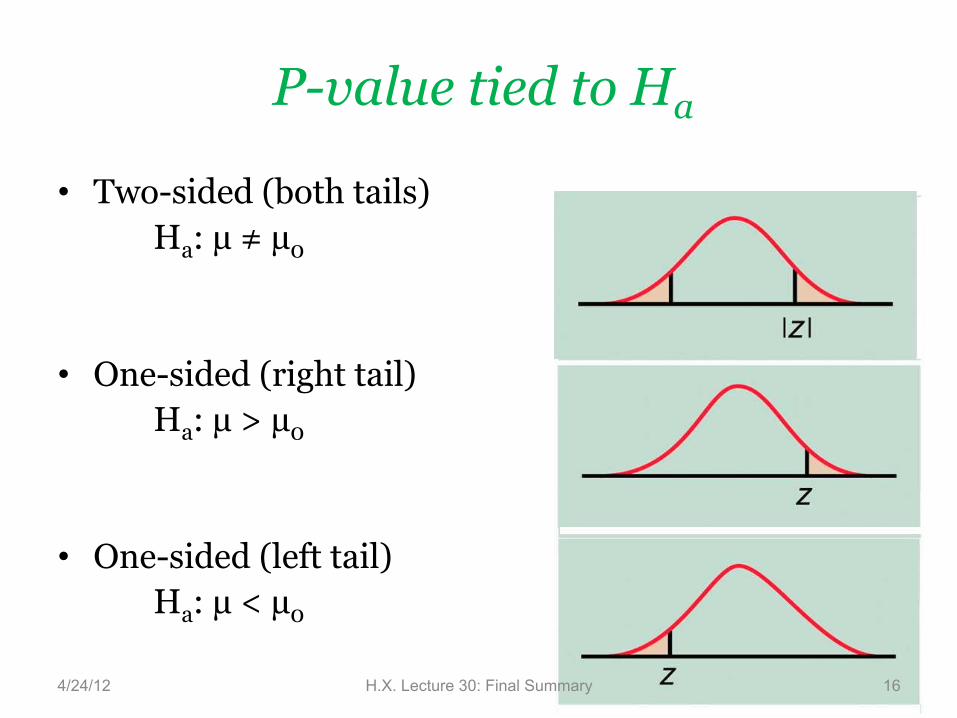
P-value tied to Ha
• Two-sided (both tails) Ha: µ ≠ µ0
• One-sided (right tail)
Ha: µ > µ0 • One-sided (left tail)
Ha: µ < µ0
4/24/12 16 H.X. Lecture 30: Final Summary
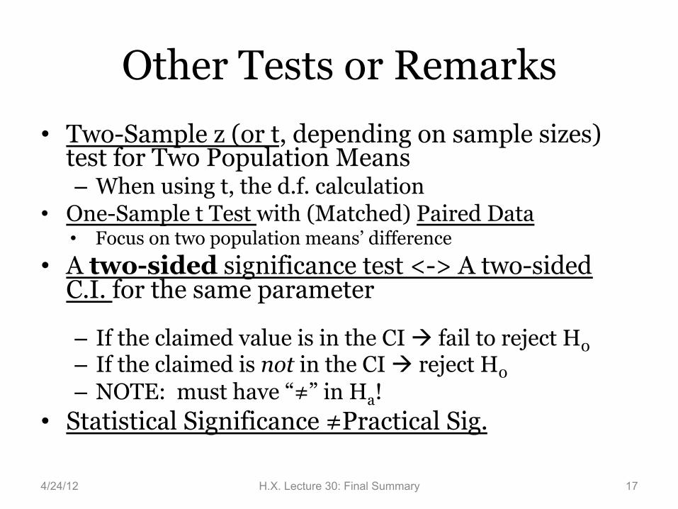
Other Tests or Remarks • Two-Sample z (or t, depending on sample sizes)
test for Two Population Means – When using t, the d.f. calculation
• One-Sample t Test with (Matched) Paired Data • Focus on two population means’ difference
• A two-sided significance test <-> A two-sided C.I. for the same parameter
– If the claimed value is in the CI à fail to reject H0 – If the claimed is not in the CI à reject H0 – NOTE: must have “≠” in Ha!
• Statistical Significance ≠Practical Sig.
4/24/12 H.X. Lecture 30: Final Summary 17
Cautions (for both C.I. and tests of significance):
• Data: assume SRS (random sampling) • Population need to be …
– If n < 30, have to check normality (by Normal QQ-plot)
– With n ≥ 30, CLT can give us approximate normality in most situations.
4/24/12 18 H.X. Lecture 30: Final Summary
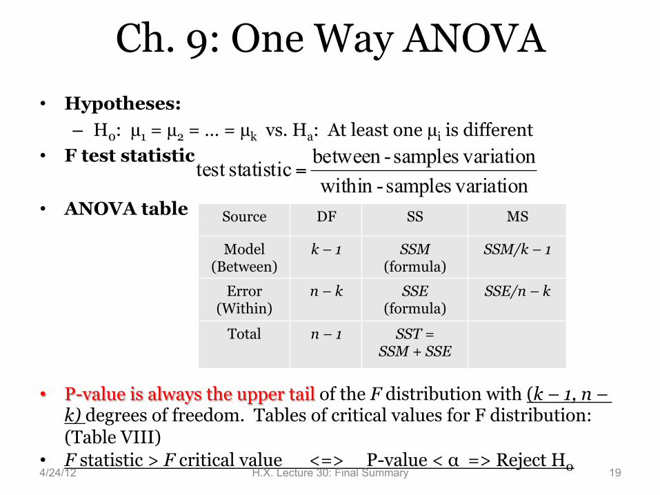
Ch. 9: One Way ANOVA • Hypotheses:
– H0: µ1 = µ2 = … = µk vs. Ha: At least one µi is different • F test statistic
• ANOVA table
• P-value is always the upper tail of the F distribution with (k – 1, n – k) degrees of freedom. Tables of critical values for F distribution: (Table VIII)
• F statistic > F critical value <=> P-value < α => Reject H0 4/24/12 H.X. Lecture 30: Final Summary 19
1. Constant variance: The variances of the k populations are the same.
– Check this with the ratio of the largest and smallest standard deviations, the ratio must be
< 2 2. Each of the k populations follows a normal
distribution. – Check this by looking at QQplots for each group
• Remark: statistical significance ≠ practical
significance 4/24/12 H.X. Lecture 30: Final Summary 20
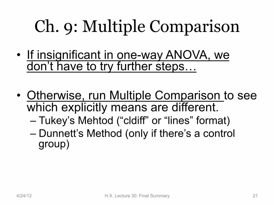
Ch. 9: Multiple Comparison
• If insignificant in one-way ANOVA, we don’t have to try further steps…
• Otherwise, run Multiple Comparison to see which explicitly means are different. – Tukey’s Mehtod (“cldiff” or “lines” format) – Dunnett’s Method (only if there’s a control
group)
4/24/12 H.X. Lecture 30: Final Summary 21
9.4: Randomized Complete Block Design
• RCBD (both treatment and block factor must be categorical)
• In RCBD, – we are only interested in the treatment factor – The block factor might affect response but that’s not of interest.
• Two F tests – Blocking Effect? Use test statistic and P-value to conclude… – Treatment Effect? Use test statistic and P-value to conclude…
4/24/12 H.X. Lecture 30: Final Summary 22
Source DF SS MS Factor A
(treatment) a – 1 SSA MSA
Factor B (block)
b – 1 SSB MSB
Error (a – 1)(b – 1) SSE MSE
Total ab – 1 SST
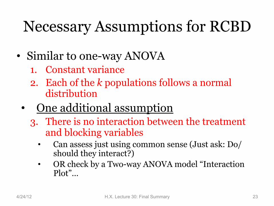
Necessary Assumptions for RCBD
• Similar to one-way ANOVA 1. Constant variance 2. Each of the k populations follows a normal
distribution • One additional assumption
3. There is no interaction between the treatment and blocking variables
• Can assess just using common sense (Just ask: Do/should they interact?)
• OR check by a Two-way ANOVA model “Interaction Plot”…
4/24/12 23 H.X. Lecture 30: Final Summary
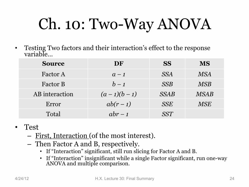
Ch. 10: Two-Way ANOVA • Testing Two factors and their interaction’s effect to the response
variable…
• Test – First, Interaction (of the most interest). – Then Factor A and B, respectively.
• If “Interaction” significant, still run slicing for Factor A and B. • If “Interaction” insignificant while a single Factor significant, run one-way
ANOVA and multiple comparison.
4/24/12 H.X. Lecture 30: Final Summary 24
Source DF SS MS
Factor A a – 1 SSA MSA
Factor B b – 1 SSB MSB
AB interaction (a – 1)(b – 1) SSAB MSAB
Error ab(r – 1) SSE MSE
Total abr – 1 SST
Ch. 10 (Cont.): Two-Way ANOVA • Interaction plot
– Roughly speaking, there’s no “Interaction” effect if all lines are parallel to each other
• In summary, for Ch. 9 and 10 we should know:
– All of One-way ANOVA (Ch. 9) • By hand and/or using SAS
– Most of randomized Blocking design (Sec 9.4), Two-way ANOVA
(Ch. 10, Section 2) • For both:
– Complete ANOVA tables, calculate DFs and F test statistic – Perform F tests using F table – Interpret SAS output
• Know the general concept of a higher order (multi-way) ANOVA model.
4/24/12 H.X. Lecture 30: Final Summary 25
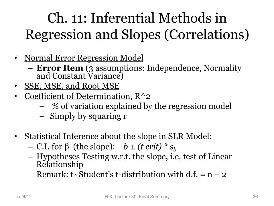
Ch. 11: Inferential Methods in Regression and Slopes (Correlations)
• Normal Error Regression Model – Error Item (3 assumptions: Independence, Normality
and Constant Variance) • SSE, MSE, and Root MSE • Coefficient of Determination, R^2
– % of variation explained by the regression model – Simply by squaring r
• Statistical Inference about the slope in SLR Model:
– C.I. for β (the slope): b ± (t crit) * sb – Hypotheses Testing w.r.t. the slope, i.e. test of Linear
Relationship – Remark: t~Student’s t-distribution with d.f. = n – 2
4/24/12 H.X. Lecture 30: Final Summary 26
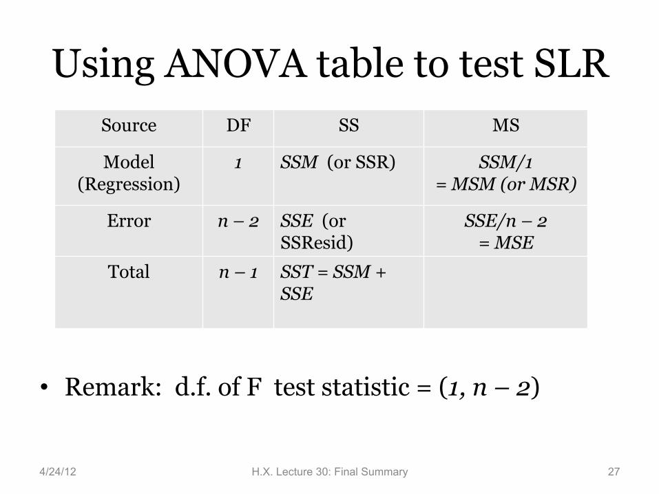
Using ANOVA table to test SLR
• Remark: d.f. of F test statistic = (1, n – 2)
4/24/12 H.X. Lecture 30: Final Summary 27
Source DF SS MS
Model (Regression)
1 SSM (or SSR) SSM/1 = MSM (or MSR)
Error n – 2 SSE (or SSResid)
SSE/n – 2 = MSE
Total n – 1 SST = SSM + SSE
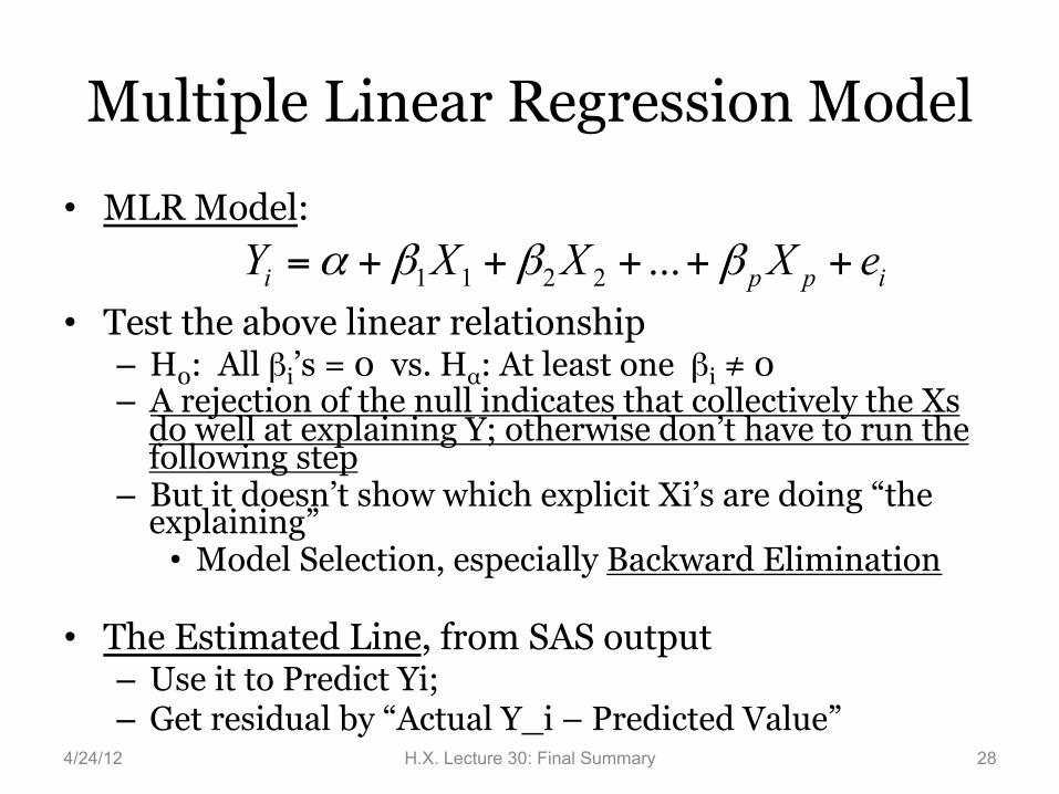
Multiple Linear Regression Model
• MLR Model:
• Test the above linear relationship – H0: All βi’s = 0 vs. Hα: At least one βi ≠ 0 – A rejection of the null indicates that collectively the Xs
do well at explaining Y; otherwise don’t have to run the following step
– But it doesn’t show which explicit Xi’s are doing “the explaining”
• Model Selection, especially Backward Elimination • The Estimated Line, from SAS output
– Use it to Predict Yi; – Get residual by “Actual Y_i – Predicted Value”
4/24/12 H.X. Lecture 30: Final Summary 28
1 1 2 2 ...i p p iY X X X eα β β β= + + + + +
After Class… • Review Notes, practices, Hw, Labs and previous tests. • Wed, Lab#8 (optional) • Final Exam (Close book, Close notes)
– Next Wed, 8-10am – Student ID, a calculator (SAT policy, NO QWERTY
keyboard) and pencils, two-page crib sheet (8” by 11”) handwritten by yourself, two-sided.
• SEE CALCULATOR POLICY and “crib sheet” (on Syllabus) from course website.
• No electronics except a calculator. Not allowed to exchange calculator or crib sheet during the exam. Not allowed to type/print your crib sheet.


![Probabilistic Reasoning [Ch. 14] Bayes Networks – Part 1 ◦Syntax ◦Semantics ◦Parameterized distributions Inference – Part2 ◦Exact inference by enumeration.](https://static.documents.pub/doc/80x56/56649f555503460f94c79016/probabilistic-reasoning-ch-14-bayes-networks-part-1-syntax-semantics.jpg)
