CH-11 Simple Linear Regression and Correlation • Empirical models •Simple linear regression •Properties of the least squares estimators •Hypothesis tests in simple linear regression •Confidence intervals •Prediction of new observations •Adequacy of the regression model
Transcript
CH-11 Simple Linear Regression andCorrelation
• Empirical models
•Simple linear regression
•Properties of the least squares estimators
•Hypothesis tests in simple linear regression
•Confidence intervals
•Prediction of new observations
•Adequacy of the regression model
11-1 Empirical Models• Many problems in engineering and science involve exploring the relationships between two or more variables.
• Regression analysis is a statistical technique that is very useful for these types of problems.
• For example, in a chemical process, suppose that the yield of the product is related to the process-operating temperature.
• Regression analysis can be used to build a model to predict yield at a given temperature level.
11-1 Empirical Models
11-1 Empirical Models
Scatter Diagram of oxygen purity versus hydrocarbon level.
Points lie scattered randomly around a straight line
11-1 Empirical Models
Based on the scatter diagram, it is probably reasonable to assume that the mean of the random variable Y is related to x by the following straight-line relationship:
where the slope and intercept of the line are called regression coefficients.
The simple linear regression model is given by
where ε is the random error term.
11-1 Empirical Models
We think of the regression model as an empirical model.
Suppose that the mean and variance of ε are 0 and σ2, respectively, then
The variance of Y given x is
If x is fixed, ε determines the properties of Y.
11-1 Empirical Models
• The true regression model is a line of mean values:
where β1 can be interpreted as the change in the mean of Y for a unit change in x.
• Also, the variability of Y at a particular value of x is determined by the error variance, σ2.
• This implies there is a distribution of Y-values at each x and that the variance of this distribution is the same at each x.
11-1 Empirical Models
The distribution of Y for a given value of x for the oxygen purity-hydrocarbon data.
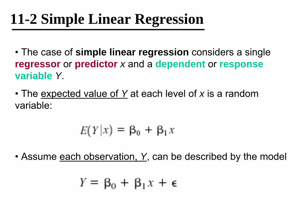
11-2 Simple Linear Regression
• The case of simple linear regression considers a single regressor or predictor x and a dependent or response variable Y.
• The expected value of Y at each level of x is a random variable:
• Assume each observation, Y, can be described by the model
11-2 Simple Linear Regression
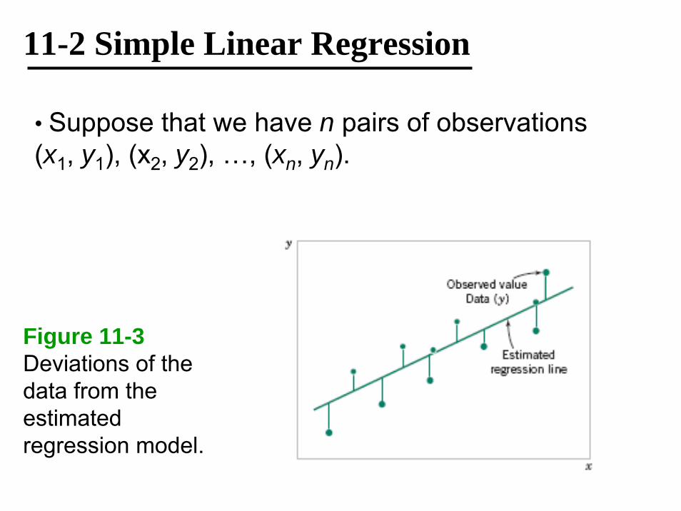
• Suppose that we have n pairs of observations (x1, y1), (x2, y2), …, (xn, yn).
Figure 11-3Deviations of the data from the estimated regression model.
11-2 Simple Linear Regression
• The method of least squares is used to estimate the parameters, β0 and β1 by minimizing the sum of the squares of the vertical deviations.
Figure 11-3Deviations of the data from the estimated regression model.
11-2 Simple Linear Regression
• n observations in the sample can be expressed as
• The sum of the squares of the deviations of the observations from the true regression line is
11-2 Simple Linear Regression
11-2 Simple Linear Regression
11-2 Simple Linear Regression
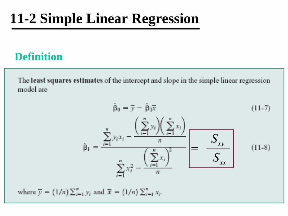
Definition
xy
xx
SS
=
11-2 Simple Linear Regression
Notation
1( )( )
n
xy i ii
S y y x x=
= − −∑
11-2 Simple Linear Regression Example 11-1
11-2 Simple Linear Regression
Example 11-1
11-2 Simple Linear Regression
Example 11-1
Figure 11-4 Scatter plot of oxygen purity y versus hydrocarbon level x and regression model
ŷ = 74.20 + 14.97x.
11-2 Simple Linear Regression
11-2 Simple Linear Regression
Estimating σ2
The error sum of squares is
The expected value of the error sum of squares is
E(SSE) = (n – 2)σ2.
11-2 Simple Linear Regression Estimating σ2
An unbiased estimator of σ2 is
where SSE can be easily computed using
2 2
1 1
where ( )n n
T i ii i
SS y y y ny= =
= − = −∑ ∑ 2is the total sum of squares of y.
11-2 Simple Linear Regression
2σ̂
2 2 2 2
1 1
1
2
( ) 170044.5321 20(92.1605) 173.376895
ˆ 173.376895 14.94748(10.17744) 21.2498141488
21.2498141488ˆ 1.182 18
n n
T i ii i
E T xy
E
SS y y y ny
SS SS S
SSn
β
σ
= =
= − = − = − =
= − = − =
= = =−
∑ ∑
ExampleConsider the data in Example 11-1. Find
1̂10.17744 14.94748
0.68088xy
xx
S
S
β= =
=Calculated before
Given before
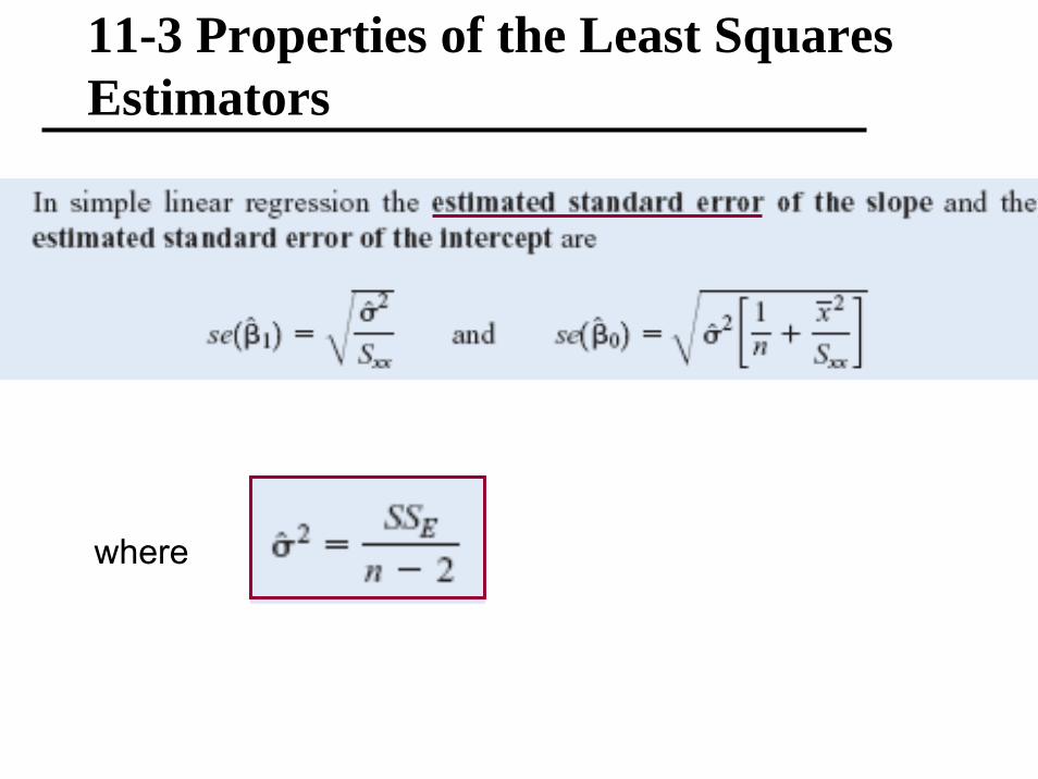
11-3 Properties of the Least Squares Estimators
• Slope Properties
• Intercept Properties
11-3 Properties of the Least Squares Estimators
where
11-4 Hypothesis Tests in Simple Linear Regression
11-4.1 Use of t-Tests
2i
2i 0 1 i
21 1
ε are NID(0, )
Y are NID( + x , )ˆ is NID( , )xxS
σ
β β σ
β β σ
11-4 Hypothesis Tests in Simple Linear Regression
11-4.1 Use of t-Tests
Suppose we wish to test
An appropriate test statistic would be
with n-2 degrees of freedom
11-4 Hypothesis Tests in Simple Linear Regression
11-4.1 Use of t-Tests
We would reject the null hypothesis if
The test statistic could also be written as:
11-4 Hypothesis Tests in Simple Linear Regression
11-4.1 Use of t-TestsSuppose we wish to test
An appropriate test statistic would be
with n-2 degrees of freedom
11-4 Hypothesis Tests in Simple Linear Regression
11-4.1 Use of t-Tests
We would reject the null hypothesis if
11-4 Hypothesis Tests in Simple Linear Regression
11-4.1 Use of t-TestsAn important special case of the hypotheses of β1 is
These hypotheses relate to the significance of regression.
Failure to reject H0 is equivalent to concluding that there is no linear relationship between x and Y.
11-4 Hypothesis Tests in Simple Linear Regression
The hypothesis H0: β1 = 0 is not rejected.
11-4 Hypothesis Tests in Simple Linear Regression
The hypothesis H0: β1 = 0 is rejected.
11-4 Hypothesis Tests in Simple Linear Regression
Example 11-2
11-4 Hypothesis Tests in Simple Linear Regression
11-4.2 Analysis of Variance Approach to Test Significance of Regression
The analysis of variance identity is
Symbolically,
Regression sum
of squaresError sum
of squares
Total corrected
sum of squares
Degrees of freedom: n-1 1 n-2
11-4 Hypothesis Tests in Simple Linear Regression
11-4.2 Analysis of Variance Approach to Test Significance of Regression
If the null hypothesis, H0: β1 = 0 is true, the statistic
follows the F1,n-2 distribution and we would reject if f0 > fα,1,n-2.
11-4 Hypothesis Tests in Simple Linear Regression
11-4.2 Analysis of Variance Approach to Test Significance of Regression
The quantities, MSR and MSE are called mean squares.
Analysis of variance table:
SSR
SST
11-4 Hypothesis Tests in Simple Linear Regression
Example 11-3
11-4 Hypothesis Tests in Simple Linear Regression
11-5 Confidence Intervals
11-5.1 Confidence Intervals on the Slope and Intercept
Definition
11-6 Confidence Intervals
Example 11-4
11-5 Confidence Intervals 11-5.2 Confidence Interval on the Mean Response
0
0
| 1 0 1
22 0
|
ˆ ˆˆ ( ) cov( , ) 0
( )1ˆ( )
Y x
Y xxx
y x x Y
x xVn S
μ β β
μ σ
= + − =
⎡ ⎤−= +⎢ ⎥
⎣ ⎦
11-5 Confidence Intervals
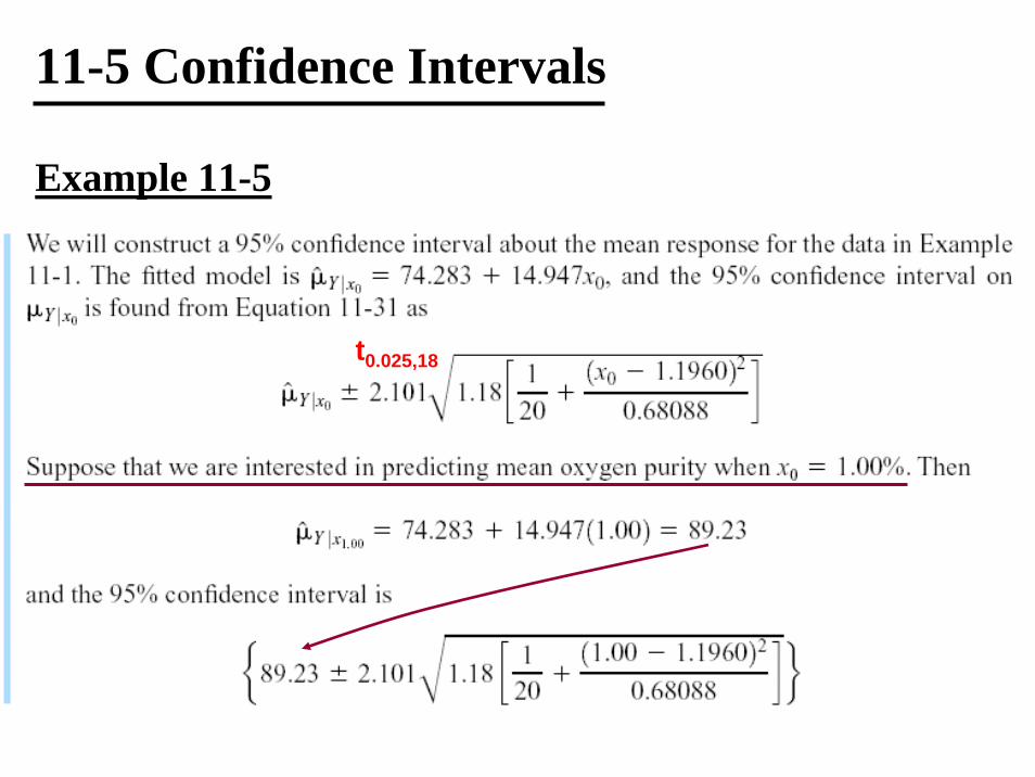
Example 11-5
t0.025,18
11-5 Confidence Intervals
Example 11-5
11-5 Confidence Intervals
Example 11-5
11-5 Confidence Intervals Example 11-5
Scatter diagram of oxygen purity data with fitted regression line and 95 percent confidence limits on μY|x0.
The width of the confidenceinterval on μY|x0 increases as
increases0| |x x−
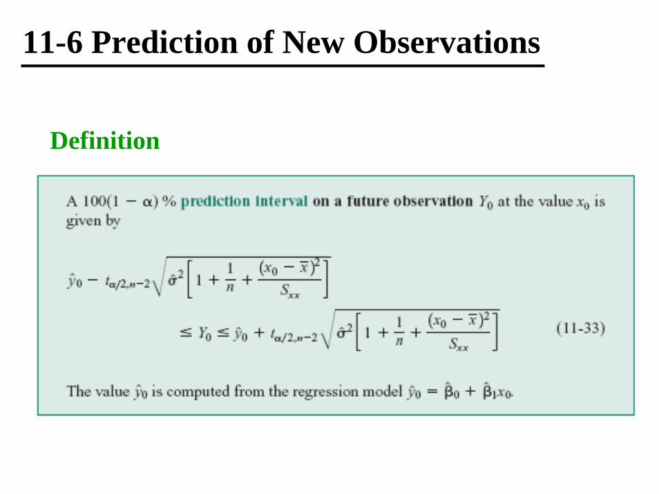
11-6 Prediction of New Observations
The point estimator of the new or future value of the response, Y0 at x0
ˆ 0 0
22 0
ˆ 0 0
ˆ
ˆ
( )1ˆ( ) ( ) 1
( ) 0
p
pxx
p
e Y Y
x xV e V Y Yn S
E e
σ
= −
⎡ ⎤−= − = + +⎢ ⎥
⎣ ⎦=
is normally distributed with mean 0 and variancep̂e ˆ( )pV e
11-6 Prediction of New Observations
Definition
11-6 Prediction of New Observations
Example 11-6
11-6 Prediction of New Observations
Example 11-6
11-6 Prediction of New Observations
Example 11-6
Scatter diagram of oxygen purity data withfitted regression line, 95% prediction limits (outer lines) , and 95% confidence limits on μY|x0.
11-7 Adequacy of the Regression Model
• Fitting a regression model requires several assumptions.
1. Errors are uncorrelated random variables with mean zero;
2. Errors have constant variance; and,
3. Errors be normally distributed.
• The analyst should always consider the validity of these assumptions to be doubtful and conduct analyses to examine the adequacy of the model
11-7 Adequacy of the Regression Model
11-7.1 Residual Analysis
• The residuals from a regression model are ei = yi - ŷi , where yiis an actual observation and ŷi is the corresponding fitted value from the regression model.
• Analysis of the residuals is frequently helpful in checking the assumption that the errors are approximately normally distributed with constant variance, and in determining whether additional terms in the model would be useful.
•Plot the residuals- in time sequence, - against ŷi- against xi