Notes on using the forecasting template: All values in blue cells are to be entered by the user, all other values are be altered. Most often this is the Actual column. Each forecast model has a all values before proceeding with your own data. Cells with red marks in the upper right corner have comments, let the mouse h further explain the template model. This spreadsheet is locked/protected in order to keep the cells with equation be altered, the spreadsheet first needs to be unlocked/unprotected. Do this click on "Tools", highlight "Protection", and select "Unprotect Sheet". The be made. Equations for models will be given when available.
Transcript
Notes on using the forecasting template:
All values in blue cells are to be entered by the user, all other values are automatically calculated, and do not need to be altered. Most often this is the Actual column. Each forecast model has a sample value set entered, make sure to clear all values before proceeding with your own data.
Cells with red marks in the upper right corner have comments, let the mouse hover over those cells to read the comments to further explain the template model.
This spreadsheet is locked/protected in order to keep the cells with equations from being changed. If a model does need to be altered, the spreadsheet first needs to be unlocked/unprotected. Do this by selecting the workbook you wish to unlock, click on "Tools", highlight "Protection", and select "Unprotect Sheet". The sheet will then be unlocked so alterations can be made.
Equations for models will be given when available.
Weighted Moving Average (3 period)
Weight 3 Weight 2 Weight 1Least Recent Most Recent
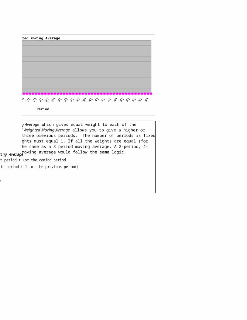
As opposed to the Simple Moving Average which gives equal weight to each of the preceding values, the 3-period Weighted Moving Average allows you to give a higher or lower weight to each of the three previous periods. The number of periods is fixed at 3, and the sum of the weights must equal 1. If all the weights are equal (for the 3-period 0.33) this is the same as a 3 period moving average. A 2-period, 4-period or n-period weighted moving average would follow the same logic.
3-Period Weighted Moving AverageF t = Forecast for period t (or the coming period )A t-1 = Actual demand in period t-1 ( or the previous period )w = WeightF t=w1 A t−1+w2 A t−2+w3 A t−3
1=w1+w2+w3
B4
Weight given to the period furthest from the new forecast.
D4
Weight given to the period immediately preceding the forecast.
As opposed to the Simple Moving Average which gives equal weight to each of the preceding values, the 3-period Weighted Moving Average allows you to give a higher or lower weight to each of the three previous periods. The number of periods is fixed at 3, and the sum of the weights must equal 1. If all the weights are equal (for the 3-period 0.33) this is the same as a 3 period moving average. A 2-period, 4-period or n-period weighted moving average would follow the same logic.
3-Period Weighted Moving AverageF t = Forecast for period t (or the coming period )A t-1 = Actual demand in period t-1 ( or the previous period )w = WeightF t=w1 A t−1+w2 A t−2+w3 A t−3
The problem with the previous two methods, Simple Moving Average and Weighted Moving Average is that a large amount of historical data is required. With Single Exponential Smoothing the oldest piece of data is eliminated once a new piece has been added. The forecast is calculated by using the previous forecast, as well as the previous actual value with a weighting or smoothing factor, alpha. Alpha can never to be greater than 1 and higher values of alpha put more weight on the most recent periods. Note on the equations below the similarity to the 3-period weighted moving average.
Simple Exponential SmoothingF t = Forecast for period t ( or the coming period )F t-1 = Forecast for period t-1 (or the previous period )A t-1 = Actual demand in period t-1 (or the previous period )α = Smoothing constant
F t=α*A t−1+ (1−α )*Ft−1
andF t−1=α*A t−2+(1−α )*F t−2
substituting F t−1 i nto the equation for F t
F t=α*A t−1+ (1−α )∗[α*A t−2+(1−α )*F t−2 ]substituting F t−2 i nto the equation for F t
F t=α*A t−1+ (1−α )∗[α*At−2+(1−α )∗{α*A t−3+(1−α )*F t−3 }]simplifying
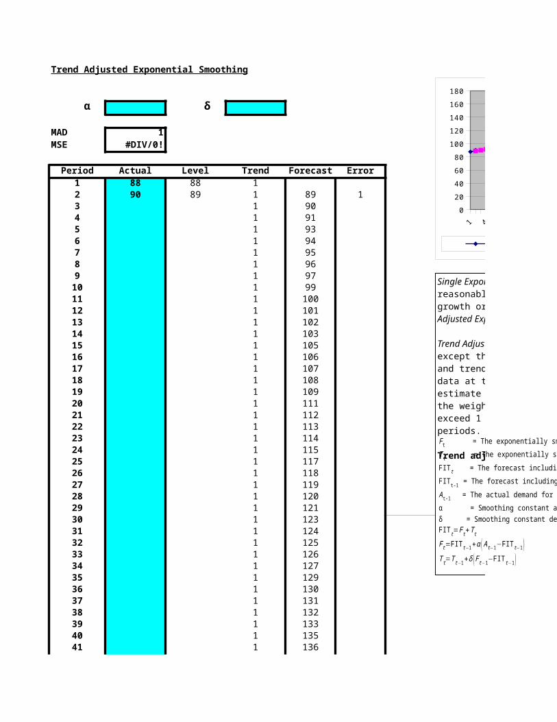
Single Exponential Smoothing assumes that the data fluctuate around a reasonably stable mean (no trend or consistent pattern of growth or decline). If the data contains a trend, the Trend Adjusted Exponential Smoothing model should be used.
Trend Adjusted Exponential Smoothing works much like simple smoothing except that two components must be updated each period: level and trend. The level is a smoothed estimate of the value of the data at the end of each period. The trend is a smoothed estimate of average growth at the end of each period. Again, the weighting or smoothing factors, alpha and delta can never exceed 1 and higher values put more weight on more recent time periods.
Trend adjusted exponential smoothing
F t = The exponentially smoothed forecast for period tT t = The exponentially smoothed trend for period tFIT t = The forecast including trend for period tFIT t-1 = The forecast including trend made for the prior periodA t-1 = The actual demand for the prior periodα = Smoothing constant alphaδ = Smoothing constant deltaFIT t=F t+T t
F t=FIT t−1+α ( A t−1−FIT t−1 )T t=T t−1+δ (F t−1−FIT t−1)
B4
Smoothing Constant Alpha determines the level of smoothing and the speed of reaction to differences between forecasts and actual occurrences
D4
Smoothing Constant Delta reduces the impact of the error that occurs between the actual value and the forecasted one
Single Exponential Smoothing assumes that the data fluctuate around a reasonably stable mean (no trend or consistent pattern of growth or decline). If the data contains a trend, the Trend Adjusted Exponential Smoothing model should be used.
Trend Adjusted Exponential Smoothing works much like simple smoothing except that two components must be updated each period: level and trend. The level is a smoothed estimate of the value of the data at the end of each period. The trend is a smoothed estimate of average growth at the end of each period. Again, the weighting or smoothing factors, alpha and delta can never exceed 1 and higher values put more weight on more recent time periods.
Trend adjusted exponential smoothing
F t = The exponentially smoothed forecast for period tT t = The exponentially smoothed trend for period tFIT t = The forecast including trend for period tFIT t-1 = The forecast including trend made for the prior periodA t-1 = The actual demand for the prior periodα = Smoothing constant alphaδ = Smoothing constant deltaFIT t=F t+T t
F t=FIT t−1+α ( A t−1−FIT t−1 )T t=T t−1+δ (F t−1−FIT t−1)
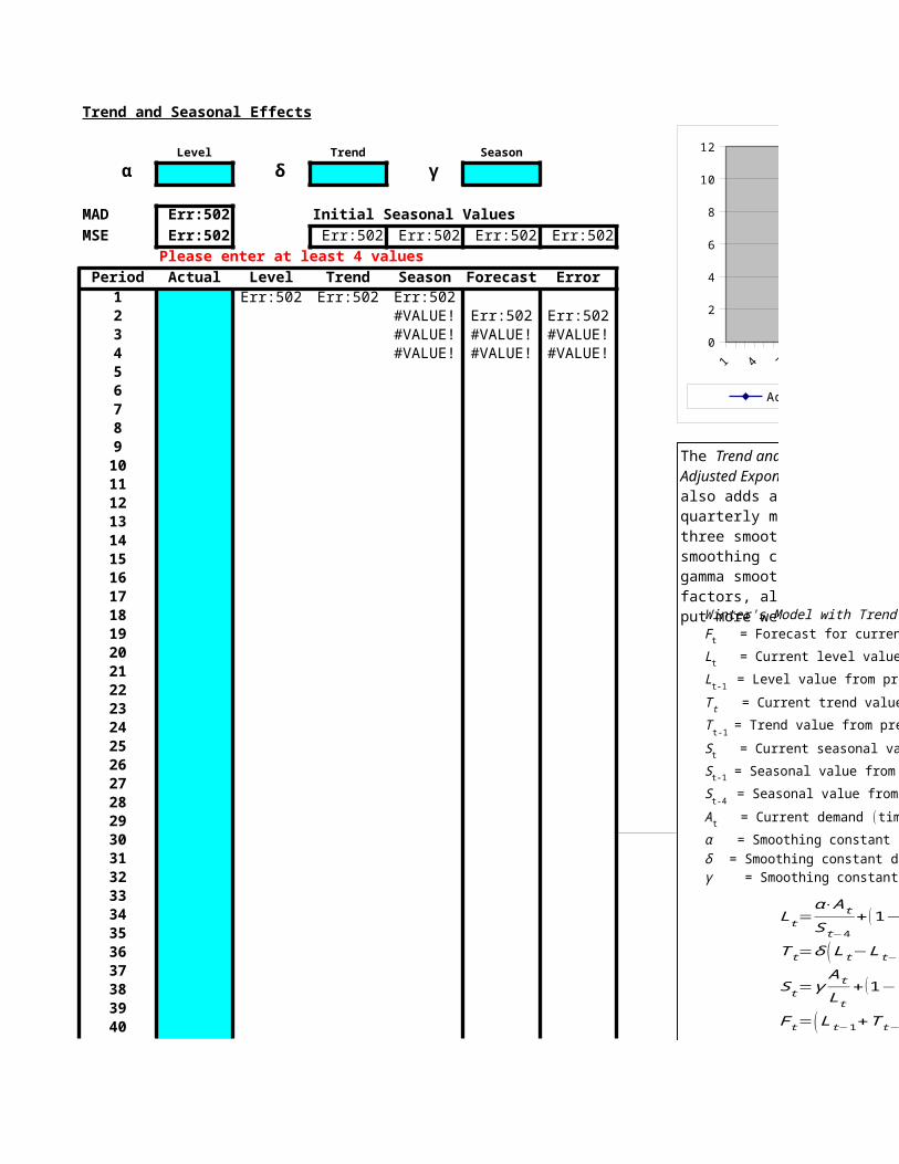
The Trend and Seasonal forecasting model is an extension of the Trend Adjusted Exponential Smoothing model. In addition to a trend, the model also adds a smoothed adjustment for seasonality. This template is a quarterly model, where the number of seasons is set to 4. There are three smoothing constants associated with this model. Alpha is the smoothing constant for the basic level, delta smoothes the trend, and gamma smoothes the seasonal index. Again, the weighting or smoothing factors, alpha, delta and gamma can never exceed 1 and higher values put more weight on more recent time periods.
Note: For initial calculations, when St-4 has not yet been calculated, the Initial Seasonal Values are used. The calculation for these is done further down on the page, starting on cell A73.
Winter's Model with Trend and Seasonal EffectsF t = Forecast for current periodLt = Current level valueLt-1 = Level value from previous periodT t = Current trend valueT t-1 = Trend value from previous periodS t = Current seasonal valueS t-1 = Seasonal value from previous periodS t-4 = Seasonal value from previous season (1 year ago = 4 periods )A t = Current demand ( time t )α = Smoothing constant alphaδ = Smoothing constant deltaγ = Smoothing constant gamma
Lt=α⋅A t
St−4+ (1−α ) (Lt−1+T t−1 )
T t=δ ( Lt−Lt−1 )+(1−δ )⋅T t−1
St=γA t
Lt+(1−γ )⋅S t−1
F t=(Lt−1+T t−1 )⋅St−4
B4
Alpha is used to smooth the basic level
D4
Delta is the smoothing constant for the trend
F4
Gamma is used for smoothing the seasonal index
4142434445464748495051525354555657585960
This area is used to compute 'initial seasonal values' due to their complexity
The Trend and Seasonal forecasting model is an extension of the Trend Adjusted Exponential Smoothing model. In addition to a trend, the model also adds a smoothed adjustment for seasonality. This template is a quarterly model, where the number of seasons is set to 4. There are three smoothing constants associated with this model. Alpha is the smoothing constant for the basic level, delta smoothes the trend, and gamma smoothes the seasonal index. Again, the weighting or smoothing factors, alpha, delta and gamma can never exceed 1 and higher values put more weight on more recent time periods.
Note: For initial calculations, when St-4 has not yet been calculated, the Initial Seasonal Values are used. The calculation for these is done further down on the page, starting on cell A73.
Winter's Model with Trend and Seasonal EffectsF t = Forecast for current periodLt = Current level valueLt-1 = Level value from previous periodT t = Current trend valueT t-1 = Trend value from previous periodS t = Current seasonal valueS t-1 = Seasonal value from previous periodS t-4 = Seasonal value from previous season (1 year ago = 4 periods )A t = Current demand ( time t )α = Smoothing constant alphaδ = Smoothing constant deltaγ = Smoothing constant gamma
Lt=α⋅A t
St−4+ (1−α ) (Lt−1+T t−1 )
T t=δ ( Lt−Lt−1 )+ (1−δ )⋅T t−1
St=γA t
Lt+(1−γ )⋅S t−1
F t=(Lt−1+T t−1 )⋅St−4
The Trend and Seasonal forecasting model is an extension of the Trend Adjusted Exponential Smoothing model. In addition to a trend, the model also adds a smoothed adjustment for seasonality. This template is a quarterly model, where the number of seasons is set to 4. There are three smoothing constants associated with this model. Alpha is the smoothing constant for the basic level, delta smoothes the trend, and gamma smoothes the seasonal index. Again, the weighting or smoothing factors, alpha, delta and gamma can never exceed 1 and higher values put more weight on more recent time periods.
Note: For initial calculations, when St-4 has not yet been calculated, the Initial Seasonal Values are used. The calculation for these is done further down on the page, starting on cell A73.
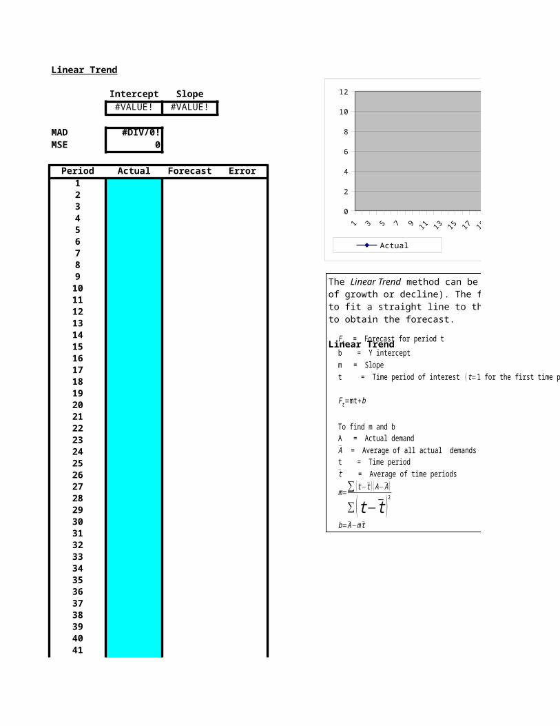
The Linear Trend method can be used if the data contains a trend (consistent pattern of growth or decline). The forecasts are calculated using least squares regression to fit a straight line to the data. This line can be extrapolated into the future to obtain the forecast.
Linear Trend
F t = Forecast for period tb = Y interceptm = Slopet = Time period of interest ( t=1 for the first time period )
F t=mt+b
To find m and bA = Actual demandA = Average of all actual demandst = Time periodt = Average of time periods
m=∑ (t − t ) ( A− A )
∑ (t− t )2
b= A−m t
B4
The Intercept is the value estimated at period 0
C4
The Slope is the amount the forecast raises with each period
The Linear Trend method can be used if the data contains a trend (consistent pattern of growth or decline). The forecasts are calculated using least squares regression to fit a straight line to the data. This line can be extrapolated into the future to obtain the forecast.
Linear Trend
F t = Forecast for period tb = Y interceptm = Slopet = Time period of interest ( t=1 for the first time period )
F t=mt+b
To find m and bA = Actual demandA = Average of all actual demandst = Time periodt = Average of time periods