CHAPTER 2 VIRTUAL SOUTHERN ANDES

10

CHAPTER 2 THE VIRTUAL SOUTHERN ANDES DATABASE

2.1 Digital image data 2.1.1 Remote sensing data Remote sensing, in general, is a process wherein information about an object is acquired without touching it (Carr, 1995). Remote sensed data used in this work include digital satellite images and air photos, both making use of the visible portion of the electromagnetic spectrum and, with respect to satellite imagery, the infrared portion of the electromagnetic spectrum. Satellite images used in this work have been acquired by the current Landsat Thematic Mapper (TM) satellite1, which is a so called passive remote sensor because it does not emit actively electromagnetic energy by its own. Instead, it uses the solar radiation reflected from the earths surface (Carr, 1995). In this work, satellite images from Landsat TM 7 with ground resolutions of 15 – 30 m have been used for morphotectonic studies. For special tectonic purposes, where higher resolutions are required than satellite images provide, high resolution (5 – 10 m) gray-scale and color air photos have been used. Satellite images as well as air photos have been projected into UTM 19 S coordinates using the PSAD 1956 ellipsoid. For coverage and examples of remote sensing data see Appendix I.

2.1.2 Digital elevation models A digital elevation model (DEM) is a digital representation of the Earth’s surface. DEMs permit visualization of topography and a more detailed and systematic search for topographic features than it is possible directly from conventional topographic contour maps. A combination of DEM with visual information from other sources like air photos and satellite images and with structural data derived from field work is a

1 Landsat 7 was launched in 1999, satellite operator is the US Geological Survey (USGS). Landsat 7 is equipped with eight photoelectric detectors (Enhanced Thematic Mapper Plus, ETM+) to image seven different bands of the electromagnetic spectrum: band 1 0.450-0.515�m (blue to cyan), band 2 0.525-0.605�m (green to orange), band 3 0.630-0.690�m (red), band 4 0.750-0.900�m (near infrared), band 5 1.55-1.75�m (short wave infrared), band 6 10.4-12.5�m (thermal infrared), band 7 2.09-2.35�m (long wave infrared), and Pan 0.52-0.90 (panchromatic). The spatial resolution, by means of pixel resolution, of Landsat 7 ETM+ images is 30m in bands 1-5 and 7, 60m in band 6, and 15m in the panchromatic band.

CHAPTER 2 VIRTUAL SOUTHERN ANDES

11

powerful tool to study the neotectonics of an area. Apart from visualization of topographic data, DEMs provide an effective way of analyzing topography satistically. Modern GIS (Geographic Information System) technology is able to analyze digital topographic data up to continental scale fast and accurate and, by the use of simple filter techniques, to derive for example slope, relief, and aspect of the surface. For this study, two DEMs (Fig. 2.1) of the southern Andes have been derived from two independent sources of data: (1) The public domain 30 arcseconds GTOPO30 altitude grid from the USGS EROS data center (available online at http://edcdaac.usgs.gov/gtopo30/gtopo30.html) which has a ground resolution of ca. 1 km (hereafter referred to as the 1 km-DEM) and (2) a high-resolution DEM derived from digitized isocontours from 1:50.000 scale topographic maps of the Instituto Geográfico Militar (Santiago, Chile) with a ground resolution of ca. 50 m (hereafter referred to as the 50 m-DEM). The 1 km-DEM has been used for regional topographic analysis whereas the 50 m-DEM has been preferred for morphometric analysis.

Fig. 2.1: Digital elevation models (DEMs) of the Southern Andes (lighter tones are higher): a) 1 km-DEM, b) clipping of 1 km-DEM (Vn. Callaqui), c) 50 m-DEM (same area as b). UTM 19 S projection, PSAD 1956 ellipsoid.

CHAPTER 2 VIRTUAL SOUTHERN ANDES

12

2.2 Image processing and analysis Image processing (i.e. manipulation) is a process to enhance the quality of digital images or to pronounce particular spatial or spectral frequencies. Filtering (removing information), thresholding, and classification (pattern recognition) are typical purposes of numerical processing of digital images to enhance their optical interpretation (Mayer, 1999, Carr, 1995). In this work, classical techniques like hill-shading (Ch. 2.2.1), average topography (Ch. 2.2.2), and base level mapping (Ch. 2.2.3) have been applied using modern GIS-based techniques to (1) better visualize topographic features and (2) to provide a new data base for morphometric analysis and interpretation. A spectral analysis of Landsat images has been performed in order to extract areas of present-day glaciation within the cordillera (Ch. 2.2.4). 2.2.1 The filtering technique

Generally, filtering aims to accentuate or attenuate a certain range of frequencies of data irrespective of which nature the data are. Since the data used in this work are spatial data, the frequency is a function of the location (Barthelme, 1995). Consequently, changes occurring over short distances (e.g. slope changes) are high-frequency properties whereas changes occurring over greater distances (e.g. changes in the height of a mountain range) are low-frequency properties of a spatial data set. The most common method for spatial filtering of a digital image is spatial convolution

filtering using a box filter algorithm (Burrough and McDonnell, 1998, Jähne, 1993). Spatial convolution filtering involves convolution (or mathematically overlay) between a point spread function (PSF, or convolution mask/kernel) and an image (a grid). Actually, a PSF is a two-dimensional uneven square matrix of i*j weights x of the following form (Schowengerdt, 1983):

x11 x12 x13 … x1j x21 x22 x23 … x2j x31 x32 x33 … x3j

... xi1 xi2 xi3 … xij

In the grid, every pixel is assigned a distinct intensity. The filter contains the respective weights (or multipliers) for the calculation. For every pixel of the grid, the pixel itself and its immediate neighbors are weighted (multiplied with the according value of the PSF). The weighted intensities are summed up and divided by the number of pixels of

CHAPTER 2 VIRTUAL SOUTHERN ANDES

13

the filter to assure that the convolution does not alter the average intensity of the image. The calculated intensity is then written into the center pixel of the filter into a new grid. This technique is called moving window (Van Diepen et al., 1998). By assigning different weights to the filter mask, different filter functions can be realized. Different low-pass (attenuating high-frequency information), high-pass (accentuating high-frequency information) as well as filters for the detection of linear structures (“edges”) can be designed (Pratt, 1991).

2.2.2 Hill shading

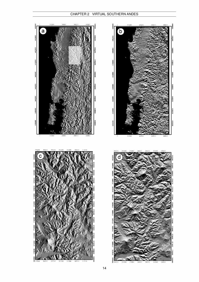
Techniques of “hill-shading” (or “shaded relief”) have been used in cartography to produce the illusion of a 3-dimensional relief map (Yoeli, 1965). During the last decades, digital image processing techniques have been developed to display DEMs as shaded relief images (Yoeli, 1967, Batson et al., 1975). The resulting images have the advantage over aerial and satellite images that they are true map projections containing no relief-induced distortion and that tonal variation are unambiguously related to relief rather than to different surface covers (vegetation, snow, volcanic ash, etc.). Hill-shading simulates the illumination and shadowing observed under different sun-angles, i.e. with different azimuths and inclinations. Thus, hill-shading enhances the high frequency information in topographic data. In this work, hill-shaded DEMs has been used in order to recognize major morphostructural features, e.g. topographic lineaments and morphotectonic units. Because structures perpendicular to the light source are better illuminated, different sun-angles were tested. Two contrasting illumination directions, E/30° and N/30°, highlight preferentially morphostructural features parallel and perpendicular to the Southern Andes, respectively (Fig. 2.2). For general purposes, e.g. for illustration, a NE/30° illumination has been used. Dependent on the scale of observation and analysis, either the 1 km-DEM or the 50 m-DEM has been processed. Fig. 2.2 (next page): Hill-shaded DEMs of the Southern Andes. 1 km-DEM illuminated from the east (a) and north (b). 50 m-DEM illuminated from the east (c) and north (d). Inclination of illumination is always 30°. Note the enhancement of margin-parallel features (for example the N-S trending Longitudinal Valley) during illumination from the east (a and c) and accentuation of oblique and orthogonal features (for example E-W striking river valleys) during illumination from the north (b and d). Inset in (a) indicates the extent of clippings c and d. UTM 19 S projection, PSAD 1956 ellipsoid.

CHAPTER 2 VIRTUAL SOUTHERN ANDES

14

CHAPTER 2 VIRTUAL SOUTHERN ANDES

15

2.2.3 Average topography Contour generalization, i.e. the projection of contours across valleys from spur to spur, is an established procedure to accentuate broader geomorphic features (Deffontaines et al., 1992) and for restoring dissected landscapes to pre-dissection forms (Pannekoek, 1967, Howard, 1973). Generalization results in the elimination of smaller valleys and other irregularities and thus smoothes the topography by filling it up. Average topography maps (Deffontaines et al., 1994) are somewhat distinct from generalized contour maps in that valleys are eliminated and peaks are lowered resulting in a smoothed and averaged topography. GIS-based filter techniques provide an objective and reproducible tool for the development of average topography maps. On the basis of the 1 km-DEM, a 5*5 low-pass filter has been used in order to obtain a smoothed map of the Southern Andes (Fig. 2.3).

Fig. 2.3: Average topography map of the Southern Andes (example): (a) Isocontour map (UTM 19 S projection, PSAD 1956 ellipsoid), (b) hill-shaded relief (illumination from N045E/45), (c) cross section (trace indicated in a). Note that there are apparent discrepancies between the original (GTOPO30) and the smoothed profile (GCM); these discrepancies occur because modeling of the average topography was made in three dimensions so that smoothing effects are influenced not only by the presence of topographic features along the profile but also by the presence of topographic features on both sides of the profile.

CHAPTER 2 VIRTUAL SOUTHERN ANDES

16

2.2.4 Base level mapping The base level is the lowest surface linking the valleys and represents a dynamic level of erosion (Deffontaines et al., 1994). This surface is conceptionally similar to the streamline surface of Dury (1951), the “Thalweg” of Annaheim (1946), and the “Reliefsockel” of Louis (1957). Base level maps illustrate the presence of principal slopes in the drainage and major knickpoints of river longitudinal profiles. Another application of the base level map is to derive the depth of dissection of the drainage system and an estimation of the minimum volume which will be eroded in future, called the available relief (Dury, 1951).

Fig. 2.4: Base level map of the Southern Andes (example): (a) Isocontour map (UTM 19 S projection, PSAD 1956 ellispsoid), (b) hillshaded relief (illumination from N045E/45), (c) cross section (trace indicated in a). Note that there are apparent discrepancies between the original (GTOPO30) and the base level profile (BLM); these discrepancies occur because modeling of the average topography was made in three dimensions so that smoothing effects are influenced not only by the presence of topographic features along the profile but also by the presence of topographic features on both sides of the profile. To construct a base level map, lines are drawn connecting points at the same altitude on neighboring streamlines. From the technical point of view, the base level map is obtained by automatic extraction of valley level points followed by altimetric data

CHAPTER 2 VIRTUAL SOUTHERN ANDES

17

interpolation. To extract valleys from the DEM numerically, the stream power index2 has been calculated from the 1 km-DEM in a first step. After this calculation, valley floors have been extracted by thresholding the stream power index grid. A binary grid has been derived consisting of pixels with stream power indices greater than 1 representing valley floors and background with pixel values smaller than 1 representing valley flanks, ridges and peaks. The coherence between the thus numerically derived drainage pattern (DEM drainage) and the real drainage pattern has been verified by comparison of the DEM drainage with hydrological maps. The binary image has then been converted into a vector file consisting of points at the center of former pixel with values greater one. To each point, the height information has been added from the DEM. From this vector data set, a TIN (triangulated irregular network) has been interpolated and finally reconverted into a grid which represents the stream line surface (Fig. 2.4). 2.2.5 Snowline extraction Modern glaciers occupy most high volcanoes and peaks in the study area and can be easily recognized on Landsat TM images by their light blue color (Fig. 2.5a). Since glacial processes may have a significant control on the topography and exhumation (e.g. Brozovic et al., 1997), the altitude of the snowline in the study area is of special scientific interest. Information regarding the distribution of modern snow/ice-fields (snowline elevation, glaciated area) has been extracted from Landsat TM images using the following routine: On band 1 from Landsat 7 TM, features having a high Albedo-reflectance (snow, ice, clouds) appear white whereas features with low Albedo-reflectance are dark. A comparison of the satellite image with geological maps and air photos allowed to distinguish between high-and low-Albedo features according to their reflectance: pixels with a reflectance higher than 230 (on a 0 - 255 scale) has been recognized as high-Albedo features whereas those pixels with a reflectance less than 230 are not covered with high-Albedo features. Using this treshold value, a binary picture highlighting snow, ice, and clouds has been derived. A manual separation between clouds and snow/ice followed in order to extract the desired information. Fig. 2.5 b shows the resulting binary picture bearing the spatial information about glaciated and snow-covered areas. By combining this information with height information from the DEM, the glacier base level (i.e. the height of the lowest part/”tongue” of the glacier/snow-

2 Stream power is defined as the rate of change of potential energy along a river and a function of discharge and slope (Burbank and Anderson, 2000).

CHAPTER 2 VIRTUAL SOUTHERN ANDES

18

field) and the flat area of several glaciers/snow-fields has been determined (Fig. 2.5 c, d and Tab. A1 in Appendix II). As is obvious from Fig. 2.5 c, the snowline decreases southward linearly as a function of latitude from ca. 2500 m at 37°S to ca. 500 m at 43°S. The respective gradient is about -250m/°S. Fig. 2.5 d shows that the area of the glaciers is inversely correlated with the snowline and increases exponentially to the south from several square kilometers at 37°S to several hundreds of square kilometer at 43°S.

Fig. 2.5: Distribution of modern glaciers in the Southern Andes extracted from spectral analysis of Landsat 7 TM images: a) Landsat 7 TM image (7-4-1- RGB, UTM 19 S projection, PSAD 1956 ellipsoid), b) resulting binary image (snow/ice appears white), c) N-S variation of the glacier base, d) N-S variation of the area covered with snow and ice (note the logarithmic scale).