Ch 5: Building Logistic Regression...

Ch 5: Building Logistic Regression Models

I Model selection

I Model checking

I Problems w/ sparse categorical data (estimators may be infinite)

226

5.1 Strategies in Model Selection

Horseshoe Crab Study

Y = whether female crab has satellites (1 = yes, 0 = No).

Explanatory variables:I WeightI WidthI Color (ML, M, MD, D) w/ dummy vars c1, c2, c3

I Spine condition (3 categories) w/ dummy vars s1, s2

227

> horseshoecrabs <-

transform(horseshoecrabs,

C = as.factor(Color),

S = as.factor(Spine))

> options(contrasts=c("contr.SAS","contr.poly"))

> crabs.fitall <-

glm((Satellites > 0) ~ C + S + Weight + Width,

family=binomial, data=horseshoecrabs)

> summary(crabs.fitall)

228

Call:

glm(formula = (Satellites > 0) ~ C + S + Weight + Width, family = binomial,

data = horseshoecrabs)

Deviance Residuals:

Min 1Q Median 3Q Max

-2.198 -0.942 0.485 0.849 2.120

Coefficients:

Estimate Std. Error z value Pr(>|z|)

(Intercept) -9.273 3.838 -2.42 0.0157

C1 1.609 0.936 1.72 0.0855

C2 1.506 0.567 2.66 0.0079

C3 1.120 0.593 1.89 0.0591

S1 -0.400 0.503 -0.80 0.4259

S2 -0.496 0.629 -0.79 0.4302

Weight 0.826 0.704 1.17 0.2407

Width 0.263 0.195 1.35 0.1779

229

(Dispersion parameter for binomial family taken to be 1)

Null deviance: 225.76 on 172 degrees of freedom

Residual deviance: 185.20 on 165 degrees of freedom

AIC: 201.2

Number of Fisher Scoring iterations: 4

230

Horseshoe Crab Study

Consider model for crabs:

logit⇥Pr(Y = 1)

⇤

= ↵+ �1c1 + �2c2 + �3c3 + �4s1 + �5s2 + �6 weight + �7 width

LR test of H0 : �1 = �2 = · · · = �7 = 0 has test statistic

-2(L0 - L1) = difference of deviances =

df = 7 p-value < 0.0001

Strong evidence at least one predictor assoc. w/ presence of satellites.

But look back at Wald tests for partial effects of weight and width.Or better, look at LR tests of all partial effects (next slide).

231

> drop1(crabs.fitall, test="Chisq")

Single term deletions

Model:

(Satellites > 0) ~ C + S + Weight + Width

Df Deviance AIC LRT Pr(>Chi)

<none> 185 201

C 3 193 203 7.60 0.055

S 2 186 198 1.01 0.604

Weight 1 187 201 1.41 0.235

Width 1 187 201 1.80 0.180

232

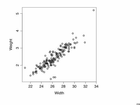
Multicollinearity

Multicollinearity (strong correlations among predictors) plays havoc withGLMs just as it does with LMs.

E.g., Corr(width, weight) = 0.89.

Is partial effect of either one relevant?Sufficient to pick one of these for a model.

> attach(horseshoecrabs)

> cor(Weight, Width)

[1] 0.88687

> plot(Width, Weight)

> detach(horseshoecrabs)

233

●

●

●

●

●

●

●

●●

●●

●

●

●

●

●

●

●

●

●

●

●

●

●

●

●

●

●●

●

●

●

●●

●

●

●

●

●

●

●

●

●

●●

●

●

●

●

●

●

●

●

●

●

●

●

●

●

●

●

●

●

●

●

●

●

●

●

●

●

●

●

●

●

●

●●

●

●

●

●

●

●

● ●

●

●

●

●

●

●●

●

●

●

●

●

●

●●

●

●●

●

●

●

●

●

●

●

●

●●

●

●

●

●

●●

●

●

●

●

●

●

●

●

●

●

●

●

●

●

●

●

●

●

●

●

●

●

●

●

●

●

●

●

●

●

●

●

●

●

●●

●

●●

●

●●

●

●

●

●

●

●

●

●

●●

●

22 24 26 28 30 32 34

23

45

Width

Weight

234

Backward Elimination

I Use W = width, C = color, S = spine as predictors.

I Start with complex model, including all interactions, say.

I Drop “least significant” (i.e., largest p-value) variable amonghighest-order terms.

I Refit model.

I Continue until all variables left are “significant”.

Note: If testing many interactions, simpler and possibly better to beginby testing all at one time as on next slide.

235

> crabs.fit1 <-

glm((Satellites > 0) ~ C*S*Width,

family=binomial, data=horseshoecrabs)

> crabs.fit2 <- update(crabs.fit1, . ~ C + S + Width)

> anova(crabs.fit2, crabs.fit1, test="Chisq")

Analysis of Deviance Table

Model 1: (Satellites > 0) ~ C + S + Width

Model 2: (Satellites > 0) ~ C * S * Width

Resid. Df Resid. Dev Df Deviance Pr(>Chi)

1 166 187

2 152 170 14 16.2 0.3

236

Horseshoe Crabs: Backward Elimination

H0: Model C+ S+W holds (has 3 parameters for C, 2 for S, 1 for W)

Ha

: Model C ⇤ S ⇤W holds, where

C ⇤ S ⇤W =

C+ S+W + (C⇥ S) + (C⇥W) + (S⇥W) + (C⇥ S⇥W)

LR stat = diff. in deviances = 186.6 - 170.4 = 16.2

df = 166 - 152 = 14 p-value = 0.30

Simpler model C+ S+W appears to be adequate.

237

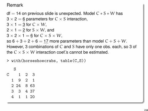
Remark

df = 14 on previous slide is unexpected. Model C ⇤ S ⇤W has3 ⇥ 2 = 6 parameters for C⇥ S interaction,3 ⇥ 1 = 3 for C⇥W,2 ⇥ 1 = 2 for S⇥W, and3 ⇥ 2 ⇥ 1 = 6 for C⇥ S⇥W,so 6 + 3 + 2 + 6 = 17 more parameters than model C+ S+W.However, 3 combinations of C and S have only one obs. each, so 3 ofthe C⇥ S⇥W interaction coef.’s cannot be estimated.

> with(horseshoecrabs, table(C,S))

S

C 1 2 3

1 9 2 1

2 24 8 63

3 3 4 37

4 1 1 20

238

Remark

In this example, we end up with the same model if we eliminate higherorder interactions 1 at a time. Try the following sequence of commandsto see this.

> drop1(crabs.fit1, test="Chisq")

> crabs.fit1a <-

update(crabs.fit1, . ~ . - C:S:Width)

> drop1(crabs.fit1a, test="Chisq")

> crabs.fit1b <- update(crabs.fit1a, . ~ . - S:Width)

> drop1(crabs.fit1b, test="Chisq")

> crabs.fit1c <- update(crabs.fit1b, . ~ . - C:Width)

> drop1(crabs.fit1c, test="Chisq")

239

Horseshoe Crabs: Backward Elimination (ctd)

At next stage, S can be dropped from model C+ S+W:

diff. in deviances = 187.46 - 186.61 = 0.85, df = 2



Model:

(Satellites > 0) ~ C + S + Width


<none> 187 201

C 3 194 202 7.81 0.05

S 2 188 198 0.85 0.66

Width 1 209 221 22.22 2.4e-06

240

> ## crabs.fit3 <- update(crabs.fit2, . ~ . - S)

> crabs.fit3 <- update(crabs.fit2, . ~ C + Width)

> deviance(crabs.fit3)

[1] 187.46

> deviance(crabs.fit2)

[1] 186.61



Model 1: (Satellites > 0) ~ C + Width

Model 2: (Satellites > 0) ~ C + S + Width


1 168 188

2 166 187 2 0.845 0.66

241



Model:

(Satellites > 0) ~ C + Width


<none> 188 198

C 3 194 198 7.0 0.072

Width 1 212 220 24.6 7e-07

> summary(crabs.fit3)

242

Call:

glm(formula = (Satellites > 0) ~ C + Width, family = binomial,


Deviance Residuals:


-2.112 -0.985 0.524 0.851 2.141

Coefficients:


(Intercept) -12.715 2.762 -4.60 4.1e-06

C1 1.330 0.853 1.56 0.119

C2 1.402 0.548 2.56 0.011

C3 1.106 0.592 1.87 0.062

Width 0.468 0.106 4.43 9.3e-06


243



AIC: 197.5


244

Horseshoe Crabs: Backward Elimination (ctd)

Results in model fit

logit(⇡) = -12.7 + 1.3c1 + 1.4c2 + 1.1c3 + 0.47 width

Forcing �1 = �2 = �3 gives

logit(⇡) = -13.0 + 1.3c+ 0.48 width

where

c =

�1, if color ML, M, MD,0, if color D.

245

> crabs.fit4 <- update(crabs.fit3, . ~ I(C == "4") + Width)



Model 1: (Satellites > 0) ~ I(C == "4") + Width

Model 2: (Satellites > 0) ~ C + Width


1 170 188

2 168 188 2 0.501 0.78

> summary(crabs.fit4)

246

Call:

glm(formula = (Satellites > 0) ~ I(C == "4") + Width, family = binomial,


Deviance Residuals:


-2.082 -0.993 0.527 0.861 2.155

Coefficients:


(Intercept) -12.980 2.727 -4.76 1.9e-06

I(C == "4")FALSE 1.301 0.526 2.47 0.013

Width 0.478 0.104 4.59 4.4e-06


247

Horseshoe Crabs Study

Conclude:I Controlling for width, estimated odds of satellite for nondark crabs

equal e1.3 = 3.7 times est’d odds for dark crabs.

95%CI :

I Given color (nondark or dark), est’d odds of satellite multiplied bye

0.478 = 1.6 for each 1 cm increase in width.

95%CI :

248

Criteria for Selecting a Model I

I Use theory, other research as guide.

I Parsimony (simplicity) is good.

I Can use a model selection criterion to choose among models.Most popular is Akaiki information criterion (AIC).

Choose model with minimum AIC where

AIC = -2L+ 2(number of model parameters)

with L = log-likelihood.

I For exploratory purposes, can use automated procedure such asbackward elimination, but not generally recommended.

R function step() will do stepwise selection procedures (forward,backward, or both).

249

Criteria for Selecting a Model II

I One published simulation study suggests > 10 outcomes of eachtype (S or F) per “predictor” (count dummy variables for factors).

Example: n = 1000, (Y = 1) 30 times, (Y = 0) 970 times

Model should contain 6 3010 = 3 predictors.

Example: n = 173 crabs, (Y = 1) 111 crabs, (Y = 0) 62 crabs

Use 6 6210 ⇡ 6 predictors.

I Can further check fit with residuals for grouped data, influencemeasures, cross validation.

250

Summarizing Predictive PowerA Correlation

For binary Y, can summarize predictive power with sample correlation ofY and ⇡.

Model Correlationcolor 0.285width 0.402color + width 0.452dark + width 0.447

251

> crabs.color <- glm((Satellites > 0) ~ C, family=binomial,

data=horseshoecrabs)

> crabs.width <- update(crabs.color, . ~ Width)

> crabs.color.width <- update(crabs.color, . ~ C + Width)

> crabs.dark.width <-

update(crabs.color, . ~ I(C == "4") + Width)

> y <- as.numeric(horseshoecrabs$Satellites > 0)

252

> pihat <- predict(crabs.color, type="response")

> cor(y,pihat)

[1] 0.28526

> pihat <- predict(crabs.width, type="response")

> cor(y,pihat)

[1] 0.40198

> pihat <- predict(crabs.color.width, type="response")

> cor(y,pihat)

[1] 0.45221

> pihat <- predict(crabs.dark.width, type="response")

> cor(y,pihat)

[1] 0.44697

253

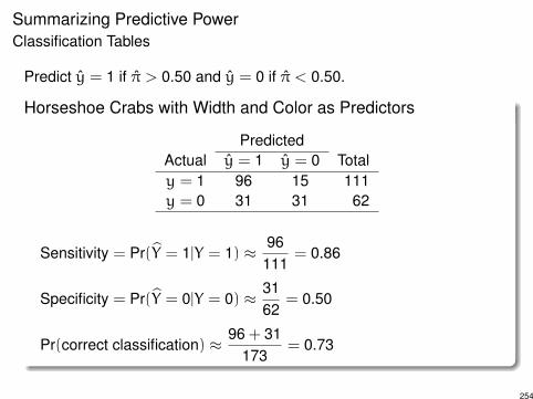
Summarizing Predictive PowerClassification Tables

Predict y = 1 if ⇡ > 0.50 and y = 0 if ⇡ < 0.50.

Horseshoe Crabs with Width and Color as Predictors

PredictedActual y = 1 y = 0 Totaly = 1 96 15 111y = 0 31 31 62

Sensitivity = Pr(bY = 1|Y = 1) ⇡ 96111

= 0.86

Specificity = Pr(bY = 0|Y = 0) ⇡ 3162

= 0.50

Pr(correct classification) ⇡ 96 + 31173

= 0.73

254

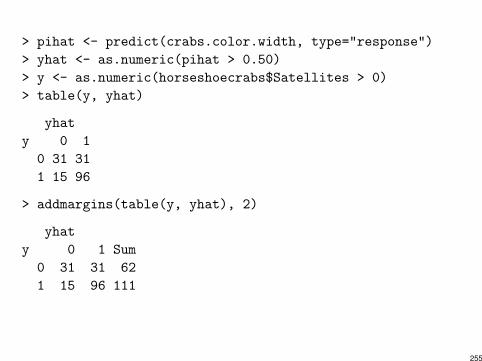
> pihat <- predict(crabs.color.width, type="response")

> yhat <- as.numeric(pihat > 0.50)


> table(y, yhat)

yhat

y 0 1

0 31 31

1 15 96

> addmargins(table(y, yhat), 2)

yhat

y 0 1 Sum

0 31 31 62

1 15 96 111

255

Remark

Table 5.3 in text actually produced by (approximate) leave-one-outcross-validation, which gives more realistic estimates. For i = 1, . . . ,n:

1. Fit the model to the data leaving out ith obs.

2. Use fitted model and x

i

to compute ⇡(i).

3. Predict yi

= 1 if ⇡(i) > 0.50 and y

i

= 0 if ⇡(i) < 0.50.



= 0.85


= 0.45


= 0.705

256

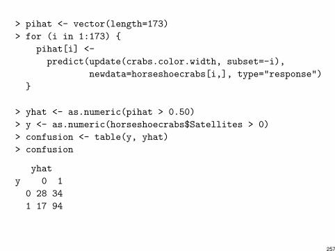
> pihat <- vector(length=173)

> for (i in 1:173) {

pihat[i] <-

predict(update(crabs.color.width, subset=-i),

newdata=horseshoecrabs[i,], type="response")

}



> confusion <- table(y, yhat)

> confusion

yhat

y 0 1

0 28 34

1 17 94

257

> prop.table(confusion, 1)

yhat

y 0 1

0 0.45161 0.54839

1 0.15315 0.84685

> sum(diag(confusion))/sum(confusion)

[1] 0.7052


> table(y,yhat)

yhat

y 0 1

0 42 20

1 37 74

258

Could use cut-offs other than ⇡0 = 0.5. E.g., for the crabs data,⇡0 = 111

173 = 0.64 (⇡ for intercept-only model).



= 0.67


= 0.68


= 0.67

Note: As cutoff ⇡0 increases, sensitivity decreases and specificityincreases.

259

Receiver Operating Characteristic (ROC) Curve

The receiver operating characteristic (ROC) curve plots sensitivityagainst 1 - specificity as the cutoff ⇡0 varies from 0 to 1.

I The higher the sensitivity for a given specificity, the better, so amodel with a higher ROC curve is preferred to one with a lowerROC curve.

I The area under the ROC curve is a measure of predictive power,called the concordance index, c.

I Models w/ bigger c have better predictive power.

Ic = 1/2 is no better than random guessing.

I If feasible, use cross-validation.

The slide after the next shows ROC curve for horseshoecrab data usingcolor and width as predictors (c = 0.77).

260

0.0 0.2 0.4 0.6 0.8 1.0

0.0

0.2

0.4

0.6

0.8

1.0

1−Specificity

Sensitivity

(Satellites > 0) ~ C + Width

262

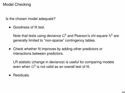
Model Checking

Is the chosen model adequate?

I Goodness of fit test.

Note that tests using deviance G

2 and Pearson’s chi-square X

2 aregenerally limited to “non-sparse” contingency tables.

I Check whether fit improves by adding other predictors orinteractions between predictors.

LR statistic (change in deviance) is useful for comparing modelseven when G

2 is not valid as an overall test of fit.

I Residuals.

263

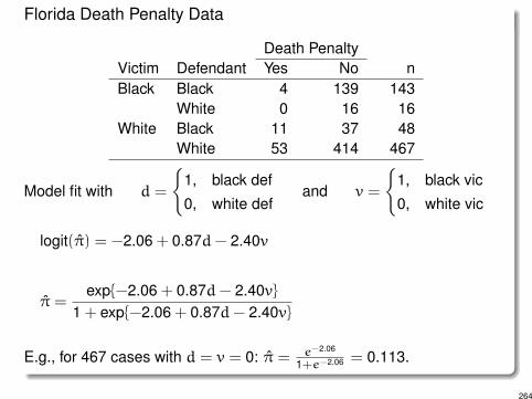
Florida Death Penalty Data

Death PenaltyVictim Defendant Yes No nBlack Black 4 139 143

White 0 16 16White Black 11 37 48

White 53 414 467

Model fit with d =

�1, black def0, white def

and v =

�1, black vic0, white vic

logit(⇡) = -2.06 + 0.87d- 2.40v

⇡ =exp{-2.06 + 0.87d- 2.40v}

1 + exp{-2.06 + 0.87d- 2.40v}

E.g., for 467 cases with d = v = 0: ⇡ = e

-2.06

1+e

-2.06 = 0.113.

264

Florida Death Penalty Data (ctd)

Fitted counts for 467 cases with d = v = 0:

”Yes”: = 52.8 ”No”: = 414.2

Corresponding observed counts are 53 “yes” and 414 “no”.

Summarizing fit over 8 cells of table:

X

2 =X (observed - fitted)2

fitted= 0.20

G

2 = 2X

(observed) log✓

observedfitted

◆= 0.38 = deviance

df = num. binomials - num. model params = 4 - 3 = 1

For H0: “model correctly specified”, G2 = 0.38, df = 1, p-value = 0.54.No evidence of lack of fit.

265

> formula(dp.fit1)

cbind(Yes, No) ~ Defendant + Victim

> deviance(dp.fit1)

[1] 0.37984

> df.residual(dp.fit1)

[1] 1

> pchisq(deviance(dp.fit1), 1, lower.tail=FALSE)

[1] 0.53769

> chisqstat(dp.fit1)

[1] 0.19779

> pchisq(chisqstat(dp.fit1), 1, lower.tail=FALSE)

[1] 0.65651

266

Remarks

I Model assumes lack of interaction between d and v in effects on Y

(homogeneous association). Adding interaction term givessaturated model, so goodness-of-fit test in this example is a test ofH0: “no interaction”. (Compare next slide to previous.)

IX

2 usually recommended over G2 for testing goodness of fit.I These tests only appropriate for grouped binary data with most

(> 80%) fitted cell counts “large” (e.g., µi

> 5).I Questionable (?) in death penalty example, where µ = 0.18 for

(v = bl, d = wh, Y = yes) and µ = 3.82 for (v = wh, d = bl,Y = yes).

I For continuous predictors or many predictors with small µi

,distributions of X2 and G

2 are not well approximated by �

2. Forbetter approx., can try grouping data before applying X

2, G2.I Hosmer-Lemeshow test forms groups using ranges of ⇡ values.

Implemented in R packages LDdiag and MKmisc and perhapsothers.

I Or can try to group predictor values (if only 1 or 2 predictors).

267

> dp.saturated <- update(dp.fit1, . ~ Defendant*Victim)

> anova(dp.fit1, dp.saturated, test="LRT")


Model 1: cbind(Yes, No) ~ Defendant + Victim

Model 2: cbind(Yes, No) ~ Defendant + Victim + Defendant:Victim


1 1 0.38

2 0 0.00 1 0.38 0.54

> anova(dp.fit1, dp.saturated, test="Rao")


Model 1: cbind(Yes, No) ~ Defendant + Victim

Model 2: cbind(Yes, No) ~ Defendant + Victim + Defendant:Victim

Resid. Df Resid. Dev Df Deviance Rao Pr(>Chi)

1 1 0.38

2 0 0.00 1 0.38 0.198 0.66

268

Residuals for Logit ModelsAt setting i of explanatory variables, let

y

i

= number of successesn

i

= number of trials (preferably ”large”)⇡

i

= estimated probability of success based on ML fit of model

Definition (Pearson residuals)

For a binomial GLM, the Pearson residuals are

e

i

=y

i

- n

i

⇡

ipn

i

⇡

i

(1 - ⇡

i

)

⇣note that X2 =

Pi

e

2i

⌘

I Dist. of ei

is approx. N(0, v) when model holds (and n

i

large),but v < 1.

I Use R function residuals() with option type="pearson".269

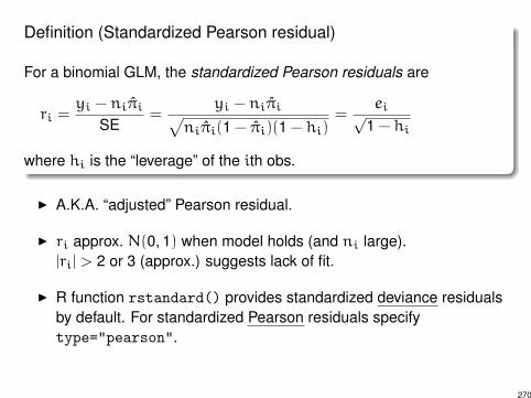
Definition (Standardized Pearson residual)

For a binomial GLM, the standardized Pearson residuals are

r

i

=y

i

- n

i

⇡

i

SE=

y

i

- n

i

⇡

ipn

i

⇡

i

(1 - ⇡

i

)(1 - h

i

)=

e

ip1 - h

i

where h

i

is the “leverage” of the ith obs.

I A.K.A. “adjusted” Pearson residual.

Ir

i

approx. N(0, 1) when model holds (and n

i

large).|ri

| > 2 or 3 (approx.) suggests lack of fit.

I R function rstandard() provides standardized deviance residualsby default. For standardized Pearson residuals specifytype="pearson".

270

Example (Berkeley Graduate Admissions)

Data on p. 237 of text.

Y = admitted into grad school at UC Berkeley (1=yes, 0=no)G = gender (g=1 female, g=0 male)D = dept (A, B, C, D, E, F)

d1 =

�1, dept B,0, o/w,

. . . , d5 =

�1, dept F,0, o/w.

For dept. A, d1 = · · · = d5 = 0.I Model

logit⇥Pr(Y = 1)

⇤= ↵+ �1d1 + · · ·+ �5d5 + �6g

seems to fit poorly (G2 = 20.2, X2 = 18.8, df = 5).Apparently there is gender ⇥ dept interaction.

271

> data(UCBAdmissions)

> is.table(UCBAdmissions)

[1] TRUE

> dimnames(UCBAdmissions)

$Admit

[1] "Admitted" "Rejected"

$Gender

[1] "Male" "Female"

$Dept

[1] "A" "B" "C" "D" "E" "F"

272

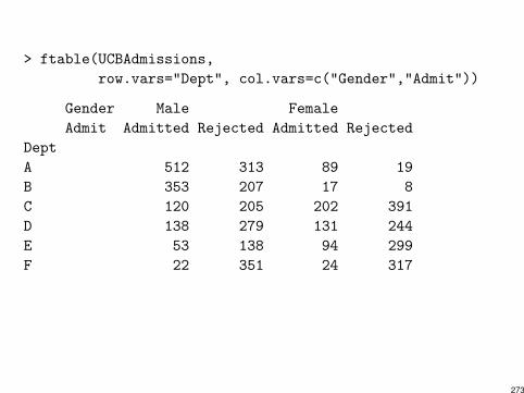
> ftable(UCBAdmissions,

row.vars="Dept", col.vars=c("Gender","Admit"))

Gender Male Female

Admit Admitted Rejected Admitted Rejected

Dept

A 512 313 89 19

B 353 207 17 8

C 120 205 202 391

D 138 279 131 244

E 53 138 94 299

F 22 351 24 317

273

Ignoring department is misleading (Simpson’s paradox):

> margin.table(UCBAdmissions, 2:1)

Admit

Gender Admitted Rejected

Male 1198 1493

Female 557 1278

> round(prop.table(margin.table(UCBAdmissions, 2:1), 1), 3)

Admit

Gender Admitted Rejected

Male 0.445 0.555

Female 0.304 0.696

> oddsratio(margin.table(UCBAdmissions, 2:1))

[1] 1.8411

274

> UCBdf <- as.data.frame(UCBAdmissions)

> head(UCBdf)

Admit Gender Dept Freq

1 Admitted Male A 512

2 Rejected Male A 313

3 Admitted Female A 89

4 Rejected Female A 19

5 Admitted Male B 353

6 Rejected Male B 207

275

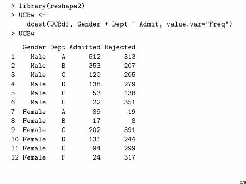
> library(reshape2)

> UCBw <-

dcast(UCBdf, Gender + Dept ~ Admit, value.var="Freq")

> UCBw

Gender Dept Admitted Rejected

1 Male A 512 313

2 Male B 353 207

3 Male C 120 205

4 Male D 138 279

5 Male E 53 138

6 Male F 22 351

7 Female A 89 19

8 Female B 17 8

9 Female C 202 391

10 Female D 131 244

11 Female E 94 299

12 Female F 24 317

276

> options(contrasts=c("contr.treatment","contr.poly"))

> UCB.fit1 <- glm(cbind(Admitted,Rejected) ~ Dept + Gender,

family=binomial, data=UCBw)

> summary(UCB.fit1)

277

Call:

glm(formula = cbind(Admitted, Rejected) ~ Dept + Gender, family = binomial,

data = UCBw)

Deviance Residuals:

1 2 3 4 5 6

-1.249 -0.056 1.253 0.083 1.221 -0.208

7 8 9 10 11 12

3.719 0.271 -0.924 -0.086 -0.851 0.205

Coefficients:


(Intercept) 0.5821 0.0690 8.44 <2e-16

DeptB -0.0434 0.1098 -0.40 0.69

DeptC -1.2626 0.1066 -11.84 <2e-16

DeptD -1.2946 0.1058 -12.23 <2e-16

DeptE -1.7393 0.1261 -13.79 <2e-16

DeptF -3.3065 0.1700 -19.45 <2e-16

GenderFemale 0.0999 0.0808 1.24 0.22

278




AIC: 103.1


279

> chisqstat(UCB.fit1)

[1] 18.824

> df.residual(UCB.fit1)

[1] 5

> pchisq(chisqstat(UCB.fit1), df.residual(UCB.fit1),

lower.tail=FALSE)

[1] 0.0020725

> UCB.fit1.stdres <- rstandard(UCB.fit1, type="pearson")

> round(UCB.fit1.stdres, 2)

1 2 3 4 5 6 7 8 9

-4.03 -0.28 1.88 0.14 1.63 -0.30 4.03 0.28 -1.88

10 11 12

-0.14 -1.63 0.30

280

> cbind(UCBw, "stdres" = round(UCB.fit1.stdres, 2))

Gender Dept Admitted Rejected stdres

1 Male A 512 313 -4.03

2 Male B 353 207 -0.28

3 Male C 120 205 1.88

4 Male D 138 279 0.14

5 Male E 53 138 1.63

6 Male F 22 351 -0.30

7 Female A 89 19 4.03

8 Female B 17 8 0.28

9 Female C 202 391 -1.88

10 Female D 131 244 -0.14

11 Female E 94 299 -1.63

12 Female F 24 317 0.30

281

Example (Berkeley Admissions Ctd)

I Standardized resids suggest Dept. A as main source of lack of fit.I Leaving out Dept. A, model with no interaction and no gender effect

fits well (G2 = 2.68, X2 = 2.69, df = 5).I In Dept. A, sample odds-ratio of admission for females vs males is

✓ = 2.86 (odds of admission higher for females).

Note: Alternative way to express model with qualitative factors is, e.g.,

logit⇥Pr(Y = 1)

⇤= ↵+ �

X

i

+ �

Z

k

,

where �

X

i

is effect of classification in category i of X.

282

> UCB.fit2 <- glm(cbind(Admitted,Rejected) ~ Dept,

family=binomial, data=UCBw,

subset=(Dept != "A"))

> summary(UCB.fit2)

283

Call:

glm(formula = cbind(Admitted, Rejected) ~ Dept, family = binomial,

data = UCBw, subset = (Dept != "A"))

Deviance Residuals:

2 3 4 5 6 8

-0.104 0.695 -0.376 0.812 -0.434 0.498

9 10 11 12

-0.518 0.395 -0.575 0.442

Coefficients:


(Intercept) 0.5429 0.0858 6.33 2.4e-10

DeptC -1.1586 0.1102 -10.52 < 2e-16

DeptD -1.2077 0.1139 -10.60 < 2e-16

DeptE -1.6324 0.1282 -12.73 < 2e-16

DeptF -3.2185 0.1749 -18.40 < 2e-16


284



AIC: 69.92


285

> chisqstat(UCB.fit2)

[1] 2.6904

> UCB.fit3 <- update(UCB.fit2, . ~ Dept + Gender)

> anova(UCB.fit2, UCB.fit3, test="Chisq")


Model 1: cbind(Admitted, Rejected) ~ Dept

Model 2: cbind(Admitted, Rejected) ~ Dept + Gender


1 5 2.68

2 4 2.56 1 0.125 0.72

286

> UCBAdmissions[,,"A"]

Gender

Admit Male Female

Admitted 512 89

Rejected 313 19

> oddsratio(UCBAdmissions[,,"A"])

[1] 0.34921

> 1/oddsratio(UCBAdmissions[,,"A"])

[1] 2.8636

287

5.3 Effects of Sparse Data

Caution: Parameter estimates in logistic regression can be infinite.

Example: S F

X

1 8 20 10 0

Model:

log✓

Pr(S)Pr(F)

◆= ↵+ �x =) e

� = sample odds-ratio =8 ⇥ 02 ⇥ 10

= 0

� = log(0) = -1

Example: Text p. 155 for multi-center trial (5 ctrs, each w/ 2 ⇥ 2 table).Two centers had no successes under either treatment arm, so estimateof center effect for these two centers is -1.

288

Infinite estimates exist when x-values where y = 1 can be “separated”from x-values where y = 0.

Example: y = 0 for x < 50 and y = 1 for x > 50.

logit⇥Pr(Y = 1)

⇤= ↵+ �x

has � = 1 (roughly speaking).

Software may not realize this!

I SAS PROC GENMOD: � = 3.84, SE = 15601054

I SAS PROC LOGISTIC gives warning.

I SPSS: � = 1.83, SE = 674.8

I R: � = 2.363, SE = 5805, with warning.

289

● ● ● ●

● ● ● ●

20 40 60 80

0.0

0.2

0.4

0.6

0.8

1.0

x

y

β

00.10.250.512

290

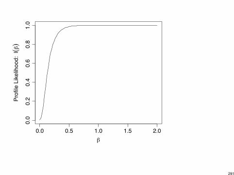
0.0 0.5 1.0 1.5 2.0

0.0

0.2

0.4

0.6

0.8

1.0

β

Prof

ile L

ikelih

ood:

l(β)

291

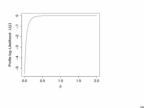
0.0 0.5 1.0 1.5 2.0

−5−4

−3−2

−10

β

Prof

ile lo

g−Li

kelih

ood:

L(β)

292

Date post:	25-Apr-2018
Category:	Documents
Upload:	lamtu
View:	214 times
Download:	1 times

Ch 5: Building Logistic Regression...

Documents